A Dynamic Approach for Operational Efficiency Improvement Using Adaptive Particle Swarm Optimization ^†

Abstract

The maritime industry is experiencing significant growth due to globalized trade, but this expansion has led to increasing environmental concerns. Studies project that shipping emissions could reach 90–130% of 2008 levels by 2050 without intervention potentially contributing up to 17% of global CO₂ emissions by 2050, thereby posing a major environmental challenge. Stringent environmental regulations from international organizations and government agencies necessitate the maritime industry to find effective solutions to reduce its greenhouse gas (GHG) emissions and improve energy efficiency. This research proposes a methodology for dynamically calculating optimal ship speed to enhance energy efficiency and reduce GHG emissions. By leveraging real-time environmental data (e.g., weather forecasts, sea state information) and operational parameters (e.g., ship characteristics, cargo load), the study utilizes an Adaptive Particle Swarm Optimization based on Velocity Information (APSO-VI) to predict optimal speed over ground (SOG) in real time. The study utilizes the Energy Efficiency Operational Index (EEOI) as a performance metric. EEOI is a widely employed measure in the maritime industry that quantifies the grams of CO₂ emitted per tonne-nautical mile (g CO₂/t nm) of transport work. The effectiveness of the proposed dynamic optimization model (APSO-VI) is assessed by comparing its performance with constant velocity models through extensive simulations, showing a 5–12% reduction in EEOI with the optimized speed model. The results demonstrate significant reductions in fuel consumption and emissions, supporting the adoption of such technologies for a more sustainable maritime industry. Future research may explore integrating machine learning techniques and advanced weather forecasting models for even more robust optimization strategies.

1. Introduction

The shipping industry has always been the heart of trade and civilization. Early civilizations arose around important water bodies and used waterways for transportation as well as for the growth of their economies since early times. With the advent of intercontinental air travel, ships are now carrying more goods than people because of increased cargo safety and cost-effectiveness when compared to air transport [1]. With globalization and internationalization of markets, the shipping industry has become one of the key enablers of world trade and shipping volumes soared.

While the maritime industry is the backbone of the supply chain and is valued at around 14 trillion USD in 2019 with promising growth forecasts irrespective of the COVID pandemic [2,3], it is responsible for almost 3% of the global greenhouse gas (GHG) emissions [4]. Studies project that shipping emissions could reach 90–130% of 2008 levels by 2050 without intervention [5]. If not regulated, the shipping industry will be responsible for over 17% of CO₂ emissions in the world by 2050 [6]. While the surge in sea trade has driven the growth of the maritime industry, it faces significant challenges due to stringent environmental regulations. Global warming and climate change have led to stricter international regulations aimed at reducing greenhouse gas emissions, with the International Maritime Organization adopting the 2023 IMO Strategy on Reduction in GHG Emissions from Ships, setting new targets including a 40% reduction in carbon intensity by 2030 and net-zero emissions “by or around 2050” [7].

Additionally, the European Union has incorporated maritime shipping into its Emissions Trading System (EU ETSs) beginning in 2024, with full implementation by 2026, requiring vessels over 5000 GT to purchase carbon allowances [8].

The main drivers for the increase in CO₂ and other climate pollutants in international maritime shipping are fleet size, increased activity of large ships, and unchanged speed over ground (SOG). Growing tonnage and operating hours also necessitate powerful engines, which lead to higher fuel consumption and, consequently, greater GHG emissions. According to the International Energy Agency (IEA), short-term emission reduction goals can be achieved by improving operational efficiency through optimized voyage speed and improved wind speed/direction assistance [9]. Optimized speed-power performance will lower fuel consumption, which in turn will reduce emissions and costs, which is vital for the economic feasibility of this transition.

2. Literature Survey

This section reviews the key methodologies and state-of-the-art techniques essential for implementing ship speed optimization, aimed at enhancing operational efficiency and minimizing emissions in the maritime industry.

2.1. Emissions and Emission Measurement

The maritime industry contributes approximately 2.5% of global CO₂ emissions, a substantial environmental concern requiring immediate attention [10]. Two critical metrics for assessing energy efficiency and emissions in maritime operations are the Energy Efficiency Design Index (EEDI) and the Energy Efficiency Operational Index (EEOI). EEDI is deployed during the design phase to ensure new vessels incorporate energy-efficient technologies [11,12], while EEOI measures operational efficiency, making it an invaluable tool for this research.

A critical parameter affecting emissions is ship resistance, which is a combination of calm water resistance and added resistance. Calm water resistance includes components such as frictional resistance, residual resistance, and air resistance. The well-defined method suggested by Holtrop and Mennen is used to calculate the ship calm water resistance [13]. Added resistance arises from external factors such as wind, waves, and currents, with ISO 15016:2015 being used as the internationally recognized method for calculating added resistance [14].

The ITTC 1978 power prediction model is widely regarded as one of the most effective and statistical methods for predicting the power delivered to ships. This model utilizes resistance calculations, open water diagrams, and propulsion tests under trial conditions to determine the delivered power, which is then used to calculate the brake power [15,16].

Reliable global weather data, available since 1979 from the European Centre for Medium-Range Weather Forecasts (ECMWFs) database, are used to predict the ship’s resistance [17].

2.2. Optimization Algorithms

Research in stochastic optimization algorithms has grown exponentially in the last decade. Many popular bio-inspired algorithms have been developed and used extensively as part of machine learning to solve complex optimization problems with non-linear constraints [18].

Particle Swarm Optimization (PSO), initially proposed by Kennedy and Eberhart in 1995, is a meta-heuristic algorithm that emulates the social behavior of birds flocking or fish schooling to locate optimal solutions in a multi-dimensional space [19]. PSO is particularly suitable for high-dimensional optimization problems due to its simplicity, robustness, and computational efficiency [20]. In the maritime navigation context, meta-heuristic methods are effective because vessel routing shares similar characteristics with the natural collective behaviors these algorithms mimic. Just as birds optimize their flight paths based on changing wind conditions and collective intelligence, ships must navigate through dynamic environmental variables (weather patterns, currents, and operational constraints) where the solution space is non-linear and multi-dimensional. The optimization process in vessel navigation involves balancing multiple competing factors (fuel consumption, time constraints, and environmental conditions) in a continuously changing environment, making PSO particularly applicable as it can efficiently search vast solution spaces without becoming trapped in local optima. However, PSO’s performance can be hampered by premature convergence and local optima entrapment [21].

Adaptive PSO (APSO) introduces adaptive parameter tuning based on particle velocity information. APSO dynamically adjusts the inertial weight using the non-linear average absolute velocity of all particles, thereby preserving swarm diversity and preventing premature convergence [22]. This research leverages APSO for real-time optimization of speed over ground (SOG).

3. Dynamic Speed Optimization Model

Dynamic speed optimization (DSO) addresses the limitations of traditional speed optimization methods, which rely on static data and precise weather forecasts, often failing to account for weather variability over time. By accurately predicting cruising speed using current weather and hull conditions, DSO can significantly reduce fuel consumption, operational costs, and greenhouse gas emissions.

3.1. Model Explanation

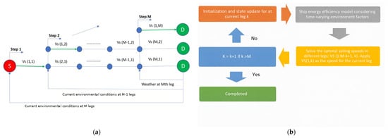
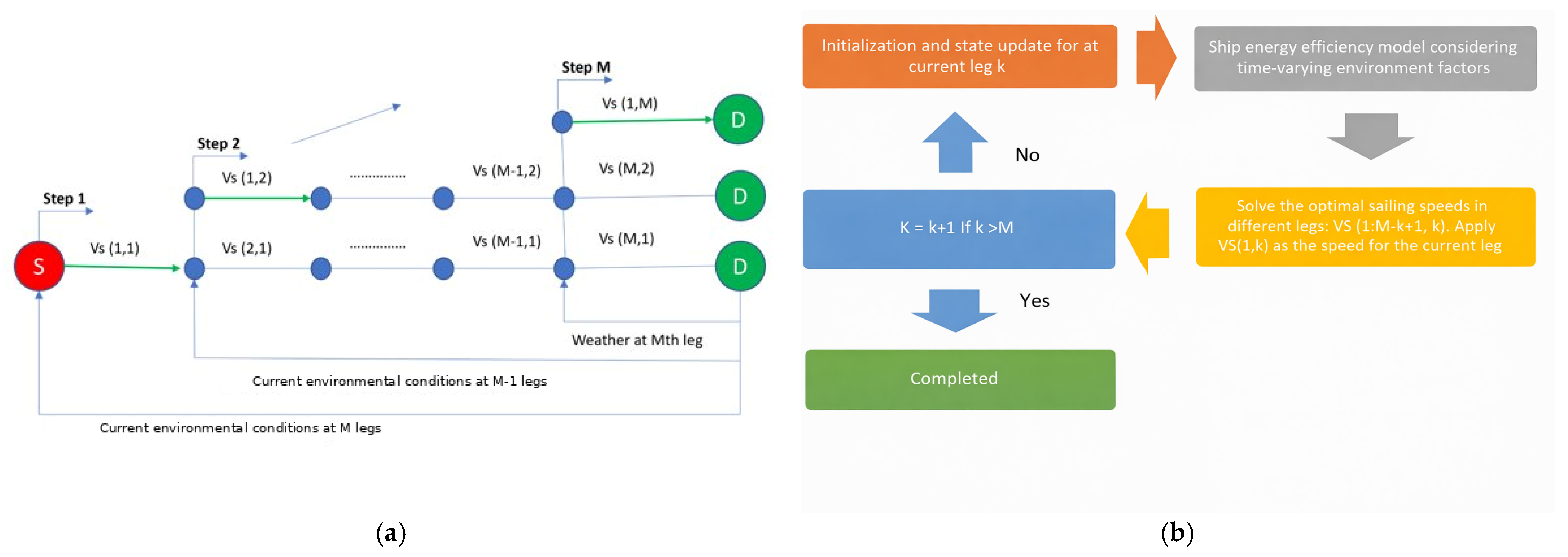
An entire route of the voyage can be broken down into “M” smaller legs. In this study, M is considered as 100. Initially, the weather conditions from the originating port to the destination port across these M legs are analyzed, and the optimal speed for each leg of the voyage based on the weather forecast made at the time of voyage start is determined through the established optimization algorithm.

Once the ship sets sail, it moves at the speed of V(1,1), which is the determined optimal speed over ground (SOG) for the first leg of the voyage. The real-time updated weather conditions are obtained at the end of leg 1 and before the start of leg 2. Applying the optimization algorithm before the start of each leg with current weather conditions helps in providing reliable speed prediction for all the remaining M-1 legs of the voyage, as shown in Figure 1a. When the ship enters leg 2, it will be sailing at the newly optimized speed of V(1,2).

Figure 1. (a) Dynamic optimization model; (b) steps involved in dynamic optimization model.

The dynamic optimization model can compensate for the unreliability of the speed optimization result caused by the unpredictability of weather conditions over time. This ensures optimal speed prediction for all the different legs of the voyage without the uncertainty added due to unreliable weather prediction made for times much ahead in the future.

The suggested dynamic speed optimization model is described through the following steps (as shown in Figure 1b):

• Measure and/or initialize the state of the system at leg k.
• Create the ship energy efficiency model considering time-varying weather conditions (mean wave period and directions, significant wave height, and U and V wind components).
• Formulate and solve the optimal ship sailing speeds in different legs under the related constraint at current leg.
• Increase k by 1 (k to k + 1) and go to step 1 until the optimization process is finished, i.e., when the ship reaches destination (when k > M).

3.2. Objective Function

For the optimization of ship energy efficiency, Energy Efficiency Operational Indicator (EEOI) is considered as the optimization objective function. EEOI for a route with j paths is calculated as follows:

$$\mathrm{EEOI} = {\displaystyle \frac{{\sum }_{\mathrm{j}}\left(\mathrm{F}{\mathrm{C}}_{\mathrm{j}}*{\mathrm{C}}_{\mathrm{F}}\right)}{\mathrm{mass}*\mathrm{D}}} \mathrm{g}/\mathrm{t} \mathrm{nm}$$

(1)

$$\mathrm{Fuel} \mathrm{consumption} \mathrm{F}{\mathrm{C}}_{\mathrm{j}} =\mathrm{SFOC}* {\mathrm{H}}_{\mathrm{j}}* \mathrm{P}{\mathrm{B}}_{\mathrm{j}}$$

(2)

where

• SFOC: specific fuel oil consumption (g/kWh) of the main engine;
• ${\mathrm{H}}_{\mathrm{j}}$: hours traveled in path j;
• $\mathrm{P}{\mathrm{B}}_{\mathrm{j}}$: brake power consumed in path j (kW);
• Mass: mass of the cargo (gross ton);
• D: total distance of the route (nm);
• ${\mathrm{C}}_{\mathrm{F}}$: conversion factor from fuel to CO₂.

The marine industry utilizes various fuel types, with Heavy Fuel Oil (HFO) being most common. For this study, HFO with a specific fuel oil consumption (SFOC) of 200 g/kWh is assumed, along with a conversion factor (${\mathrm{C}}_{\mathrm{F}}$) of 3.114 for CO₂ calculations.

For M leg route, at first step, the number of optimization variables or the dimension will be M. At the last step M, the optimization variable will be one. The optimization variable is the ship speed ${\mathrm{V}}_{\mathrm{S}}$. For dynamic optimization, the model must solve M optimization equations with variables reducing from M to 1. EEOI for a route with M legs is given as:

$$\mathrm{EEOI} = {\displaystyle \frac{{\sum }_{\mathrm{k} = 1}^{\mathrm{M}}\left(\mathrm{SFOC} * {\mathrm{H}}_{\mathrm{k}} * \mathrm{P}{\mathrm{B}}_{\mathrm{k}} * {\mathrm{C}}_{\mathrm{F}}\right)}{\mathrm{mass} * \mathrm{D}}} \mathrm{g}/\mathrm{t} \mathrm{nm}$$

(3)

Brake power in leg k depends on weather conditions and speed of the ship. Hence, brake power in leg k can be expressed as a function of speed of the vessel in leg k (${\mathrm{V}}_{\mathrm{S}}^{\mathrm{k}}$) and the weather condition $\mathrm{W}{\mathrm{C}}^{\mathrm{k}}$:

$$\mathrm{P}{\mathrm{B}}_{\mathrm{k}} = \mathrm{PB}\left({\mathrm{V}}_{\mathrm{S}}^{\mathrm{k}},\mathrm{W}{\mathrm{C}}^{\mathrm{k}}\right)$$

(4)

Since routes are divided based on distance, the distance of each leg is known. Let the distance of leg k be ${\mathrm{D}}_{\mathrm{k}}$. The hour traveled in leg k can be expressed as:

$${\mathrm{H}}_{\mathrm{k}} = {\displaystyle \frac{{\mathrm{D}}_{\mathrm{k}}}{{\mathrm{V}}_{\mathrm{S}}^{\mathrm{k}}}}$$

(5)

The objective function to be minimized is:

$$\min |\mathrm{EEOI} = {\displaystyle \frac{{\sum }_{\mathrm{k}=1}^{\mathrm{M}\text{-}\mathrm{k}+1}\left(\mathrm{SFOC}*\frac{{\mathrm{D}}_{\mathrm{k}}}{{\mathrm{V}}_{\mathrm{S}}^{\mathrm{k}}}*\mathrm{PB}\left({\mathrm{V}}_{\mathrm{S}}^{\mathrm{k}},\mathrm{W}{\mathrm{C}}^{\mathrm{k}}\right)*{\mathrm{C}}_{\mathrm{F}}\right)}{\mathrm{mass}*\mathrm{D}}}, \forall \mathrm{k}\in \left\{1,2,\dots .\right\}$$

(6)

The two major constraints for the objective function are as follows:

• The ship speed must be within minimum (${\mathrm{V}}_{\mathrm{S}} \min$) and maximum value (${\mathrm{V}}_{\mathrm{S}} \max$) of ship speed (kn): ${\mathrm{V}}_{\mathrm{S}} \min < {\mathrm{V}}_{\mathrm{S}}^{\mathrm{k}} <{ \mathrm{V}}_{\mathrm{S}} \max ,\forall \mathrm{k}\in \left\{1,2,\dots .\right\}$
• The average speed of the ship in the route must be between (${\mathrm{V}}_{\mathrm{Avg}} \min$ and ${\mathrm{V}}_{\mathrm{Avg}} \max$):${\mathrm{V}}_{\mathrm{Avg}} \min <{\displaystyle \frac{{\sum }_{\mathrm{k}=1}^{\mathrm{M}\text{-}\mathrm{k}+1}{\mathrm{V}}_{\mathrm{S}}^{\mathrm{k}}}{\mathrm{M}\text{-}\mathrm{k}+1}}<{\mathrm{V}}_{\mathrm{Avg}} \max ,\forall \mathrm{k}\in \left\{1,2,\dots .\right\}$

While the EEOI formula appears linear in its mathematical expression, the optimization problem becomes highly non-linear due to the complex relationship between ship speed and brake power consumption under varying weather conditions. The function $\mathrm{PB}\left({\mathrm{V}}_{\mathrm{S}}^{\mathrm{k}},\mathrm{W}{\mathrm{C}}^{\mathrm{k}}\right)$ incorporates complex hydrodynamic interactions between the vessel and its environment, resulting in a non-linear relationship between speed and power. Additionally, the inverse relationship between speed (${\mathrm{V}}_{\mathrm{S}}^{\mathrm{k}}$) and travel time (${\mathrm{H}}_{\mathrm{k}}$) introduces further non-linearity. These factors, combined with the dynamic nature of weather conditions across voyage legs, create a complex, multi-dimensional optimization problem that benefits from meta-heuristic approaches like APSO-VI.

3.3. Particle Swarm Optimization Parameters

This study uses Adaptive PSO based on Velocity Information (APSO-VI) to solve the dynamic optimization problem. APSO-VI eliminates the drawback of PSO, which is becoming entangled in local optima, and improves the convergence precision and speed by manifold [22].

A particle size of 100 is considered, as it gives the best results for our optimization problem. The number of iterations is set as 1000, as experimental results show that the APSO-VI algorithm can achieve the global best within 1000 iterations for high-dimensional problems [22].

4. Scenarios and Results

4.1. Simulation Setup

The route selected for this study was chosen based on criteria including intercontinental distance, variable weather conditions, and significance as a major trade corridor. A transatlantic route (New York–Amsterdam) was selected for this purpose due to its importance in global shipping. As said before, the route is divided into 100 legs with varying distance, where the weather conditions hold the same. For predicting resistance and power for each leg, a general cargo vessel is considered as the case vessel for the simulation. As mentioned in Section 2.1 Emissions and Emission Measurement, the ITTC 1978 model is well-suited for our needs in predicting power and resistance. Before the start of the first leg, a random weather condition is chosen for each leg from the 200 different weather conditions collected from ECMWF database (U and V wind components (at 10 m), significant wave height (in meters), mean wave direction, and mean wave period (in seconds)). The optimal ship sailing speeds in different legs under the related constraint at the current leg are obtained using the APSO algorithm. The obtained optimal speed for the current leg is used to sail to the next leg. This process is carried out until the ship reaches its destination. The same steps are carried out with 10 different random seeds.

4.2. Scenarios

The following two scenarios are considered for the simulation runs:

Scenario 1: The speed range for the general cargo vessel is 14–20 knots [23]. Hence, the minimum and maximum speed constraints are set at 14 knots and 20 knots. The average minimum and maximum speed are considered as 16 knots and 16.5 knots.

Scenario 2: To analyze how our algorithm works with a larger range of ship speeds, the minimum and maximum speed constraints are set at 10 knots and 20 knots. The average minimum and maximum are considered as 15 knots and 15.5 knots.

Each simulation scenario is run for 10 different seeds. Confidence interval is plotted for each evaluating parameter based on these 10 different runs, with the true mean lying in the measured interval with 95% confidence.

4.3. Performance Metrics

Our approach is compared with two constant velocity models, where the constant velocity is the average minimum and maximum speed considered for the respective scenarios. For Scenario 1, our model is compared with constant velocity models using speeds of 16 knots and 16.5 knots. Similarly, for Scenario 2, we compare with constant velocity models using speeds of 15 knots and 15.5 knots.

The main performance indicator is EEOI and the average speed for the route calculated from our approach. Through our dynamic optimization model, we obtain optimal speeds V(1,1), V(1,2) … V(1,M) for each leg of the voyage.

Let velocity at leg k (${\mathrm{V}}_{\mathrm{S}}^{\mathrm{k}}$) = ${\mathrm{V}}_{\mathrm{S}}$ (1,k) and $\mathrm{W}{\mathrm{C}}^{\mathrm{k}}$ be the weather condition (wind and wave parameters) at leg k when the ship is at leg k.

Then, the EEOI for our model is calculated as:

$$\mathrm{EEOI} = {\displaystyle \frac{{\sum }_{\mathrm{k}=1}^{\mathrm{M}}\left(\mathrm{SFOC}*\frac{{\mathrm{D}}_{\mathrm{k}}}{{\mathrm{V}}_{\mathrm{S}}^{\mathrm{k}}}*\mathrm{PB}\left({\mathrm{V}}_{\mathrm{S}}^{\mathrm{k}},\mathrm{W}{\mathrm{C}}^{\mathrm{k}}\right)*{\mathrm{C}}_{\mathrm{F}}\right)}{\mathrm{mass}*\mathrm{D}}} \mathrm{g}/\mathrm{t} \mathrm{nm}$$

(7)

For the constant velocity model:

$${\mathrm{V}}_{\mathrm{S}}^{\mathrm{k}} = \mathrm{Constant} \mathrm{speed} \forall \mathrm{k} ϵ \left(1,2 \dots . \mathrm{M}\right)$$

(8)

This constant ${\mathrm{V}}_{\mathrm{S}}^{\mathrm{k}}$ is used in the EEOI equation above to calculate EEOI for the constant velocity model.

The average speed for our dynamic model is calculated as:

$$\mathrm{Average} \mathrm{velocity} = {\displaystyle \frac{{\sum }_{\mathrm{k}=1}^{\mathrm{M}}{\mathrm{V}}_{\mathrm{S}}^{\mathrm{k}}}{\mathrm{M}}}$$

(9)

These performance metrics allow us to directly compare the efficiency gains achieved through dynamic speed optimization versus conventional constant speed operation.

4.4. Results

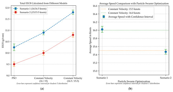
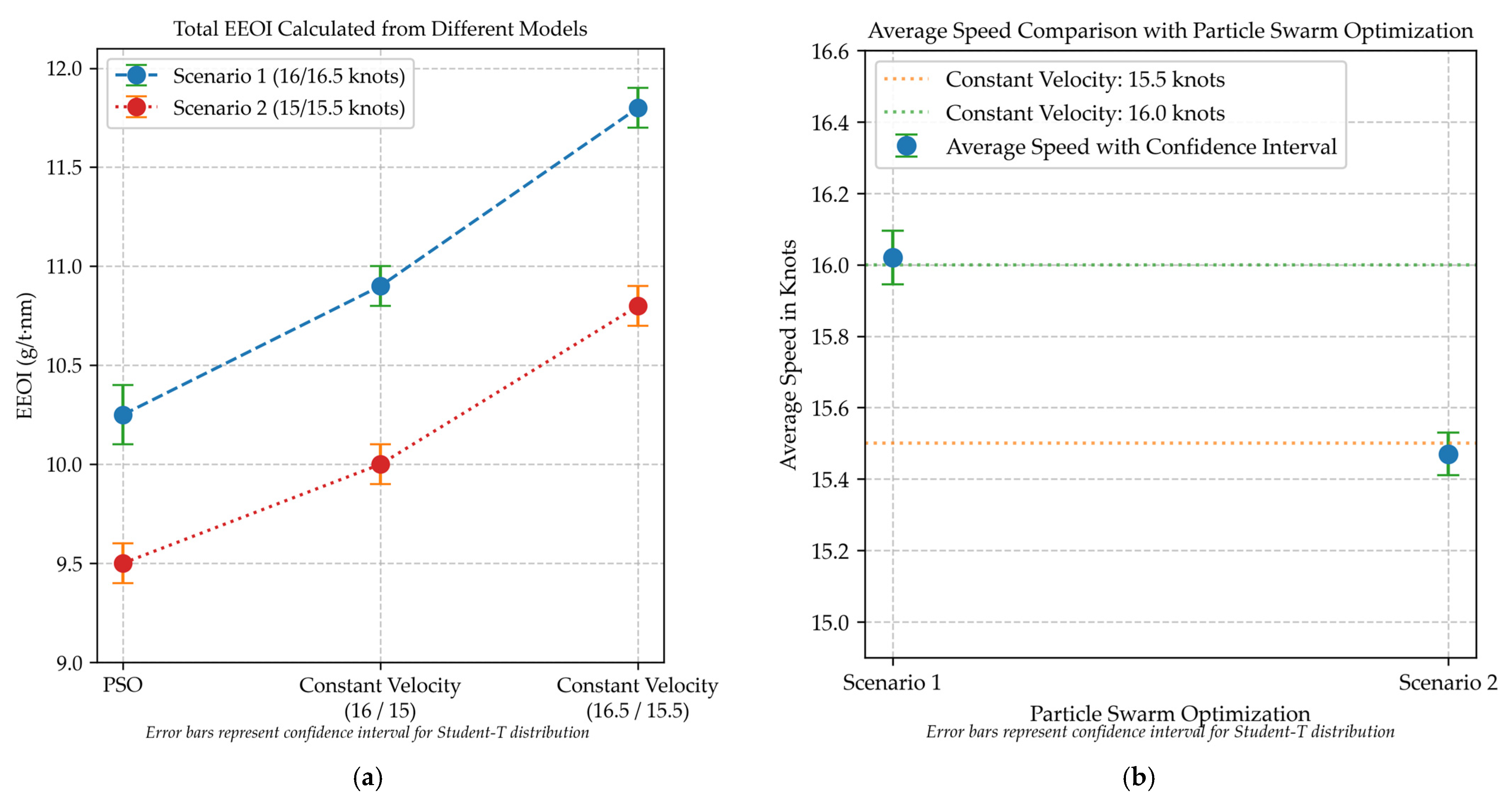
Scenario 1: For the transatlantic route, the EEOI obtained from the PSO model ranges from 10.125 g/t nm to 10.375 g/t nm (as shown in Figure 2a), which is notably lower than the constant velocity models at 16 and 16.5 knots. The average speed ranges from 15.9 kn to 16.1 kn (as shown in Figure 2b). The difference in EEOI between the constant velocity (16 kn) model and our PSO model is approximately 0.6 g/t nm.

Figure 2. Results comparison: (a) comparison of EEOI for various models with Scenario 1 and Scenario 2; (b) average speed comparison with particle swarm optimization.

This 0.6 g/t nm EEOI difference accounts for reduced fuel consumption:

(0.6 * mass * Distance)/C_F = (0.6 * 37,200 * 3900)/3.144 = 27,953.76 kg = 30.81 tonnes

(10)

The average reduction in EEOI for Scenario 1 is approximately 5%.

Scenario 2: For the transatlantic route, the EEOI obtained from the PSO model ranges from 9.4 g/t nm to 9.6 g/t nm (as shown in Figure 2a), which is significantly lower than the constant velocity models at 15 and 15.5 knots. The average speed ranges from 15.49 kn to 15.54 kn (as shown in Figure 2b). The difference in EEOI between the constant velocity (15.5 kn) model and our PSO model is approximately 1.4 g/t nm.

This 1.4 g/t nm EEOI difference accounts for reduced fuel consumption:

(1.4 * mass * Distance)/C_F = (1.4 * 37,200 * 3900)/3.144 = 65,225.43 kg = 71.90 tonnes

(11)

The average reduction in EEOI for Scenario 2 is approximately 12%.

5. Conclusions and Future Work

Climate change and growing emissions are topics of worldwide concern, and with GHG emissions from ships increasing exponentially, action is desperately needed. This research began with the hypothesis that conventional static speed models fail to account for the dynamic nature of maritime environments, resulting in suboptimal energy efficiency. We proposed that a dynamic approach using advanced meta-heuristic algorithms could better respond to changing conditions and significantly improve operational efficiency.

Our key contribution is the development of a novel dynamic speed optimization framework that

• Integrates real-time environmental data with vessel characteristics;
• Employs APSO-VI to continuously recalculate optimal speed profiles;
• Demonstrates significant practical improvements in EEOI metrics.

The proposed dynamic speed optimization helps to reduce fuel consumption and, in turn, emissions and costs. The speed prediction model proposed by optimizing the Energy Efficiency Operational Index proves to be an effective solution.

The average percentage of EEOI reduced for the transatlantic route with a speed range of 10–20 knots is approximately 12%. Similarly, the average percentage of EEOI reduced for the same route with a speed range of 14–20 knots is approximately 5%. This clearly shows that increasing the speed range increases the search space of velocities and thus helps to calculate a more optimized result using APSO.

Contemporary research has explored various methodologies to augment operational efficiency in the maritime sector. The convergence of machine learning techniques with optimization algorithms has shown significant promise in improving prediction accuracy and optimizing operational parameters. Advanced weather forecasting models and real-time data analytics further bolster the robustness and efficacy of these optimization strategies.

Recent industry implementations provide further validation for speed optimization approaches. Maersk implemented speed optimization across its container fleet in 2022–2023, reporting a 9.3% reduction in fuel consumption and associated CO₂ emissions [24]. Similarly, CMA CGM’s Smartship project—leveraging AI for route and engine optimization—has targeted CO₂ emissions reductions of 5% to 10%, aligning closely with the savings predicted in our simulation results [25].

Several studies underscore the potential of integrating operational data with machine learning algorithms to optimize vessel routes and speeds. For instance, leveraging historical operational data for predictive analytics enables a comprehensive understanding of vessel behavior, facilitating the optimization of future voyages. Such approaches have demonstrated marked improvements in fuel efficiency and emission reduction, underscoring their relevance to this research.

As industry continues to innovate and adopt these advanced methodologies, the potential for significant environmental and economic benefits becomes increasingly attainable, paving the way for a greener and more efficient future in maritime operations.

References

- Placek, M. Global Merchant Fleet-Number of Ships by Type, Statista. 2024. Available online: https://www.statista.com/statistics/264024/number-of-merchant-ships-worldwide-by-type/ (accessed on 5 May 2025).
- Karatzas, B. Maritime: The-Almost-Invisible 14 Trillion Dollars Industry, Business Daily. 2021. Available online: https://www.businessdaily.gr/apopseis/40385_maritime-almost-invisible-14-trillion-dollars-industry (accessed on 6 May 2025).
- Shipping and World Trade: Driving Prosperity. International Chamber of Shipping. 2022. Available online: https://www.ics-shipping.org/shipping-fact/shipping-and-world-trade-driving-prosperity/ (accessed on 9 May 2025).
- Review of Maritime Transport 2024. UN Trade and Development (UNCTAD). 2024. Available online: https://unctad.org/publication/review-maritime-transport-2024#:~:text=faster%20renewal%20of%20the%20world’s,capacity%20for%20the%20first%20time (accessed on 6 May 2025).
- Fourth Greenhouse Gas Study 2020. International Maritime Organization. 2020. Available online: https://www.imo.org/en/OurWork/Environment/Pages/Fourth-IMO-Greenhouse-Gas-Study-2020.aspx (accessed on 6 May 2025).
- Aviation and Shipping Emissions in Focus. European Environment Agency. 2021. Available online: https://www.eea.europa.eu/articles/aviation-and-shipping-emissions-in-focus (accessed on 6 May 2025).
- International Maritime Organization (IMO). Resolution MEPC.377(80): 2023 IMO Strategy on Reduction of GHG Emissions from Ships; MEPC 80/17/Add.1, Annex 15; IMO: London, UK, 2023; Available online: https://wwwcdn.imo.org/localresources/en/OurWork/Environment/Documents/annex/MEPC%2080/Annex%2015.pdf (accessed on 6 May 2025).
- Directive-2023/959-en-EUR-Lex EUR. 2023. Available online: https://eur-lex.europa.eu/legal-content/EN/TXT/?uri=CELEX%3A32023L0959 (accessed on 6 May 2025).
- Cret, L.; Gauch, H.; Connelly, E.; Paoli, L. How the Shipping Sector Could Save on Energy Costs–Analysis-IEA, International Energy Agency. 2025. Available online: https://www.iea.org/commentaries/how-the-shipping-sector-could-save-on-energy-costs (accessed on 6 May 2025).
- Aryn Baker, S. The Shipping Industry Sets Sail for Net-Zero Future at COP26, Time. 2021. Available online: https://time.com/6116582/shipping-cop26-emissions/ (accessed on 6 May 2025).
- Eedi-Rational, Safe and Effective (No Date) International Maritime Organization. Available online: https://www.imo.org/fr/MediaCentre/HotTopics/Pages/EEDI.aspx (accessed on 6 May 2025).
- Jassal, R. Ship Energy Efficiency: Here Is All You Need to Know, MySeaTime. 2018. Available online: https://www.myseatime.com/blog/detail/ship-energy-efficiency (accessed on 6 May 2025).
- Holtrop, J. A statistical re-analysis of resistance and propulsion data. Int. Shipbuild. Prog. 1984, 31, 272–276. [Google Scholar]
- ISO 15016:2015; Ships and Marine Technology—Guidelines for the Assessment of Speed and Power Performance by Analysis of Speed Trial Data. International Organization for Standardization (ISO): Geneva, Switzerland, 2015.
- International Towing Tank Conference (ITTC). Performance Prediction Method; Recommended Procedures and Guidelines, 7.5-02-03-01.1 (ITTC 1978 Power Prediction Method). In Proceedings of the 15th ITTC, Hague, The Netherlands, 3–10 September 1978. [Google Scholar]
- Helma, S.; Streckwall, H.; Richter, J. The Effect of Propeller Scaling Methodology on the Performance Prediction. J. Mar. Sci. Eng. 2018, 6, 60. [Google Scholar] [CrossRef] [Scilit]
- European Centre for Medium-Range Weather Forecasts. ECMWF. 2025. Available online: https://www.ecmwf.int/ (accessed on 9 May 2025).
- Darwish, A. Bio-Inspired Computing: Algorithms Review, Deep Analysis, and the Scope of Applications. Future Comput. Inform. J. 2018, 3, 231–246. [Google Scholar] [CrossRef] [Scilit]
- Tam, A. A Gentle Introduction to Particle Swarm Optimization, MachineLearningMastery.com. 2021. Available online: https://machinelearningmastery.com/a-gentle-introduction-to-particle-swarm-optimization/ (accessed on 9 May 2025).
- Lee, K.Y.; Park, J.-B. Application of particle swarm optimization to economic dispatch problem: Advantages and disadvantages. In Proceedings of the 2006 IEEE PES Power Systems Conference and Exposition, Atlanta, Georgia, 29 October–1 November 2006; pp. 188–192. [Google Scholar]
- Rahman, I.; Vasant, P.M.; Singh, B.S.M.; Abdullah-Al-Wadud, M. On the performance of accelerated particle swarm optimization for charging plug-in hybrid electric vehicles. Alex. Eng. J. 2016, 55, 419–426. [Google Scholar] [CrossRef] [Scilit]
- Xu, G. An adaptive parameter tuning of particle swarm optimization algorithm. Appl. Math. Comput. 2013, 219, 4560–4569. [Google Scholar] [CrossRef] [Scilit]
- Solutions, M.E. Basic Principles of Ship Propulsion; MAN Energy Solutions: Copenhagen, Denmark, 2023. [Google Scholar]
- 2023 Maersk Sustainability Report (2024) Sustainability Reports. Available online: https://www.maersk.com/~/media_sc9/maersk/corporate/sustainability/files/resources/2023/maersk-sustainability-report-2023.pdf (accessed on 9 May 2025).
- 2023 CSR Report—CMACGM 2023 Sustainability Report. 2024. Available online: https://www.cmacgm-group.com/en/sustainability/our-publications (accessed on 9 May 2025).
Disclaimer/Publisher’s Note: The statements, opinions and data contained in all publications are solely those of the individual author(s) and contributor(s) and not of MDPI and/or the editor(s). MDPI and/or the editor(s) disclaim responsibility for any injury to people or property resulting from any ideas, methods, instructions or products referred to in the content. |
© 2026 by the authors. Licensee MDPI, Basel, Switzerland. This article is an open access article distributed under the terms and conditions of the Creative Commons Attribution (CC BY) license.