


Abstract
A fast modelling framework is presented for loss estimation in current-source microinverters. The power stage is modelled with ideal switches and simplified magnetics to keep simulations lightweight, while dedicated estimators reconstruct core, conduction, and switching losses from simulated waveforms using Steinmetz-based and analytical models. The method is demonstrated on an interleaved active-clamp flyback with H-bridge unfolder but remains topology-agnostic and applicable to other current source (CS) DC/DC variants. Control includes maximum power point tracking (MPPT) with voltage-reference tracking, a PID loop, simplified grid synchronization, and peak-current regulation. Dynamic tests under irradiance and grid-voltage variations confirm stable operation and correct MPPT behaviour. A steady-state loss breakdown at 0.75 p.u. irradiance predicts ~97% overall efficiency, consistent with reported microinverter performance. The framework enables rapid design exploration and efficiency prediction without full device-level modelling, balancing accuracy and computational speed.
1. Introduction
The global transition from fossil-fuel-dominated systems to low-carbon energy infrastructures has become a central priority for governments, industry, and research institutions. Fossil fuels remain subject to volatile international prices and supply constraints, creating systemic vulnerabilities that ripple through economies and societies. At the same time, their combustion remains the dominant source of anthropogenic greenhouse gas emissions, directly contributing to global warming. Renewable energy sources therefore play a dual role: they enable decarbonization while simultaneously increasing energy security by diversifying supply and reducing import dependence [1]. Policy instruments in many regions, ranging from the European Union’s Green Deal to national renewable portfolio standards, reflect the strategic recognition that widespread renewable integration is a prerequisite for both climate stability and energy independence.
Among renewable generation options, photovoltaic (PV) energy stands out for its rapid cost reductions, scalability, and versatility. According to the International Energy Agency, PV is now the least-cost source of new electricity capacity in much of the world [2]. Its inherent modularity enables installations ranging from utility-scale power plants down to individual rooftop systems, with minimal site constraints and relatively short installation times. Unlike wind or hydro, PV can be integrated close to consumption points, reducing the need for extensive transmission and enabling significant contributions to decentralized and resilient energy architectures. As a result, PV accounts for the majority of new renewable installations globally, and projections consistently place it as a cornerstone of the 2050 carbon-neutral energy system [3].
At the interface between PV modules and the grid, the choice of power electronic architecture is decisive for system efficiency, cost, and reliability. Microinverters—where each module is paired with a dedicated DC-AC stage—have gained attention due to their ability to perform maximum power point tracking (MPPT) at the module level, improving yield under partial shading or mismatch [4]. Microinverters also enhance system modularity: arrays can be scaled panel by panel, installation is simplified for residential users, and fault isolation is straightforward. Nevertheless, drawbacks remain: the distributed nature of electronics increases cost per watt and complicates thermal management, while long-term reliability under harsh outdoor conditions remains a concern [5]. Despite these limitations, microinverters are widely regarded as enabling technology for expanding PV penetration in diverse environments where centralized inverters are less practical.
Within the broad class of microinverter architectures, current-source (CS) microinverters represent a distinct approach. Unlike traditional voltage-source designs, CS microinverters enforce a continuous input current from the PV panel and directly inject a shaped current into the grid [6]. Advantages include reduced requirement for bulky electrolytic capacitors, inherent short-circuit protection, and in some cases simpler modulation strategies. However, disadvantages include higher current ripple reflected into the PV source, more stringent design requirements for magnetics, and sensitivity to switching stress at high frequencies [7]. Several topologies have been proposed to implement CS inverters, including the interleaved flyback, push-pull, two-transistor forward, and resonant derivatives. Among these, the interleaved active-clamp flyback has emerged as particularly promising: interleaving reduces ripple and distributes current stress, while the active clamp both limits device overvoltage and recycles leakage energy [8,9]. This combination provides a favourable trade-off between efficiency, cost, and simplicity at the power levels relevant for module-integrated inverters.
Given the diversity of potential topologies and operating conditions, modelling and computer-aided analysis play a critical role in design optimization. High-fidelity, device-level simulations can capture switching dynamics in detail but are computationally expensive, making them unsuitable for large sweeps across PV IV curves or parametric studies under different grid voltages and frequencies [10]. A complementary approach is to employ idealized circuit models—ideal switches and averaged magnetics—to accelerate simulations, and to complement them with loss-estimation scripts that reconstruct semiconductor and core losses from measured waveforms. Such a hybrid approach allows rapid yet reasonably accurate estimation of efficiency and thermal stress, enabling both comparative topology evaluation and parametric optimization [11].
Considering these needs, this paper develops a model for fast estimation of semiconductor and magnetic losses across PV operating points and grid conditions, enabling rapid design iteration without full device-level simulation. The remainder of the paper is structured as follows. Section 2 outlines the proposed modelling framework for current-source microinverters, with emphasis on the interleaved active-clamp flyback. The section also details the custom loss-calculation blocks (core, main switch, and output diode) and the associated power-averaging methods. Section 3 verifies the approach on representative operating points, reporting efficiency curves and loss breakdowns. Section 4 concludes with key findings, limitations, and directions for future work.
2. Materials and Methods
2.1. Modelling Approach
2.1.1. Modelling Goals
The primary objective of the proposed model is to provide a framework for fast and accurate estimation of power losses in current-source microinverters under diverse operating conditions. Rather than reproducing all semiconductor switching transients explicitly, the circuit is represented with ideal switches and simplified magnetics, while auxiliary loss-estimation blocks reconstruct conduction, switching, and core losses from waveforms. This reduces simulation time by an order of magnitude compared with full device-level models, while maintaining sufficient precision for efficiency evaluation and comparative design studies. The framework allows systematic sweeps of PV operating points, as well as grid parameters, yielding loss and efficiency maps that guide design optimization. This approach is particularly relevant given the continued decline in PV module prices, which shifts attention to the efficiency and reliability of power electronics and their control, making accurate yet computationally efficient modelling increasingly valuable for design.
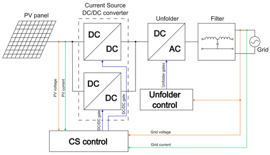
A block diagram of the proposed model is presented in Figure 1. The system consists of four main functional blocks, the PV source, a current-source (CS) DC/DC stage, a DC/AC unfolder, and the output filter connected to the grid, all coordinated by control blocks. The CS DC/DC stage is implemented here as an interleaved active-clamp flyback, which offers favourable performance in terms of ripple reduction and energy recovery. However, the framework is not limited to this topology: with minor adjustments, other current-source converters such as active-clamp forward, two-transistor flyback, or push–pull variants can be represented within the same structure. The unfolder stage, responsible for transferring energy from the intermediate DC node to the grid, is modelled as an H-bridge in this work for simplicity and generality. Nonetheless, alternative inverter topologies (e.g., half-bridge or multilevel structures) can be incorporated with minimal changes, since their function in the model is limited to shaping the injected current. This modularity highlights the general applicability of the proposed modelling framework across a broad range of current-source microinverter architectures.
Figure 1.
Block diagram of the presented model.
2.1.2. Converter Modelling
As described in the previous Section 2.1.1 the power stage can be divided into three main blocks, the modelling of which can be presented as:
PV source.
The PV model is implemented as a three-dimensional lookup table (LUT) with linear interpolation. The table returns the module current for a given terminal voltage , irradiance G (normalized 0–1), and cell temperature T. The output current drives a controlled current source connected to the CS DC/DC input, so the PV behaves with realistic I–V characteristics while remaining numerically light. The LUT is built automatically from manufacturer datasheets: raw points are extracted using the automated procedure, then fitted into a consistent I–V surface using the optimization routine of [12]. This workflow enables rapid loading and testing of different modules without re-parameterizing the circuit model. To ensure robustness in sweeps, the LUT is clamped to the physical regions and .
Current-source DC/DC stage.
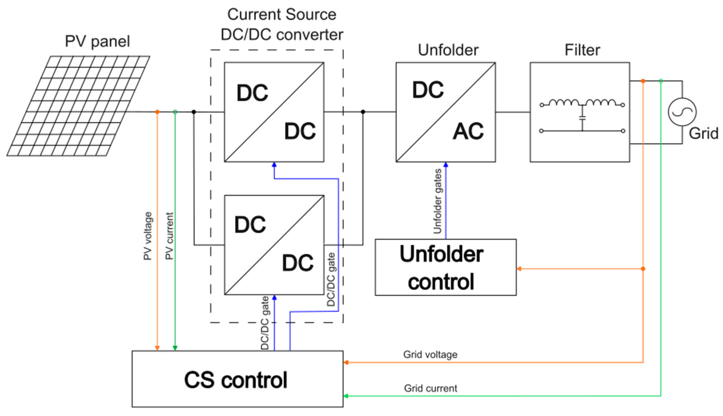
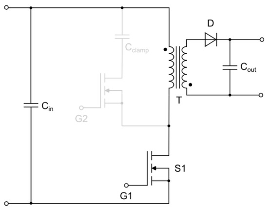
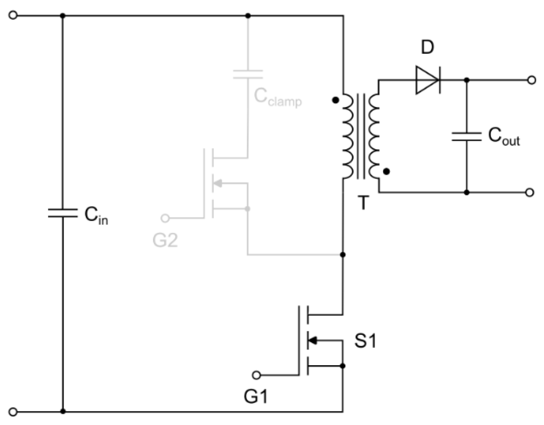
The current-source converter is implemented as an interleaved flyback, with one phase shown in Figure 2. The essential model components are highlighted in black: input capacitor , main switch , transformer , secondary diode , and output capacitor . For simplicity, the active clamp network—comprising clamp switch and capacitor shown in grey—is omitted from the functional model.
Figure 2.
Simplified schematic of one phase of the interleaved flyback CS DC/DC stage.
This simplification significantly reduces numerical stiffness and improves simulation speed, since the commutation of the clamp branch introduces high-frequency resonant transitions and nonlinear switching dynamics. The absence of explicit clamp modelling, however, has two main implications:
- Switch-voltage stress: In the real circuit, the clamp capacitor limits the peak voltage on and recycles leakage energy. In the simplified model, this protective effect is not directly simulated. Instead, switch voltage is represented as an input parameter to the loss-estimation block, which uses datasheet values or designer-selected clamp voltages to compute switching energy.
- Resonant transitions: The active clamp also provides quasi-resonant transitions that can enable zero-voltage switching (ZVS) under certain operating conditions. Since this is not represented in the simplified plant, ZVS is introduced in the loss calculation stage by a flag variable controlling whether is included or suppressed. This preserves the ability to evaluate the impact of ZVS on efficiency without adding resonant states to the main circuit.
By treating the clamp implicitly, the model balances speed and accuracy: waveforms of current and flux density remain representative of the real converter, while detailed clamp dynamics are abstracted into parameters for the loss models. This abstraction also maintains generality: with minimal adjustments the same framework can represent other CS DC/DC topologies such as active-clamp forward, two-transistor flyback, or push–pull converters.
Unfolder stage.
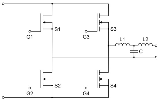
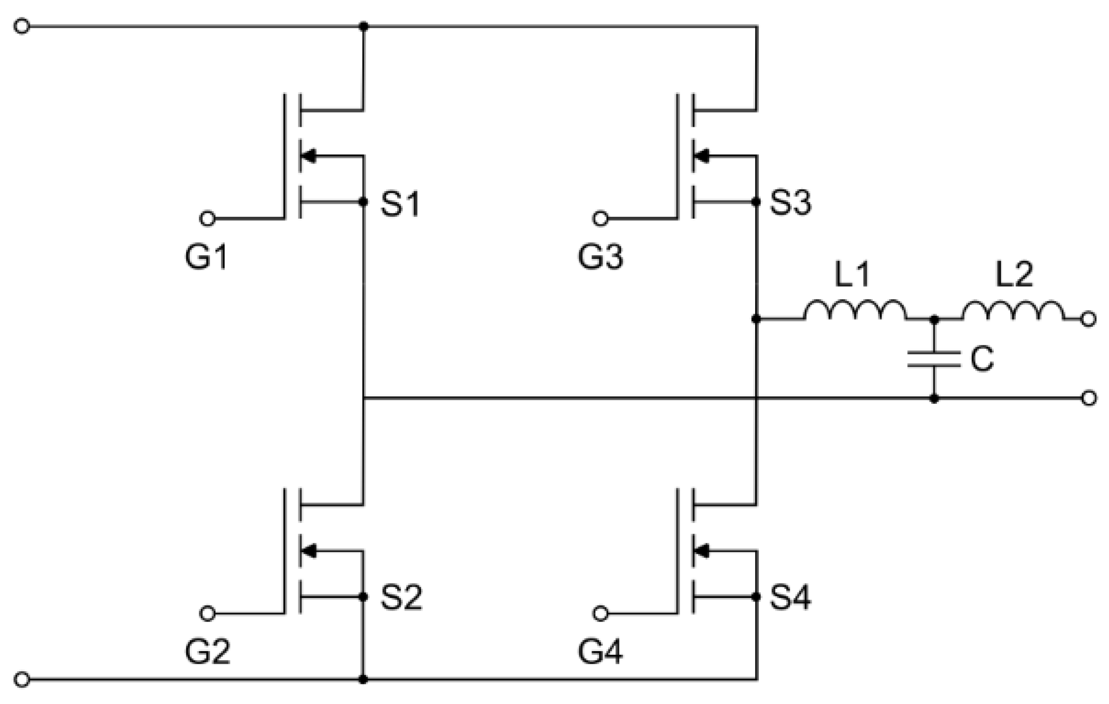
The grid unfolder is modelled as a full H-bridge, shown in Figure 3, which alternately connects the output of the CS DC/DC stage to the positive and negative half-cycles of the grid. In this configuration, the switches operate at the grid frequency only (50 Hz in this study), meaning that switching losses are negligible compared with conduction losses. Accordingly, only conduction losses are evaluated in the model, based on the RMS current through each device and its on-state resistance (or diode drop, depending on the device technology). The series filter ensures sinusoidal injection into the grid.
Figure 3.
H-bridge unfolder stage used for grid connection.
Control Modelling.
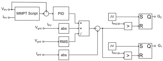
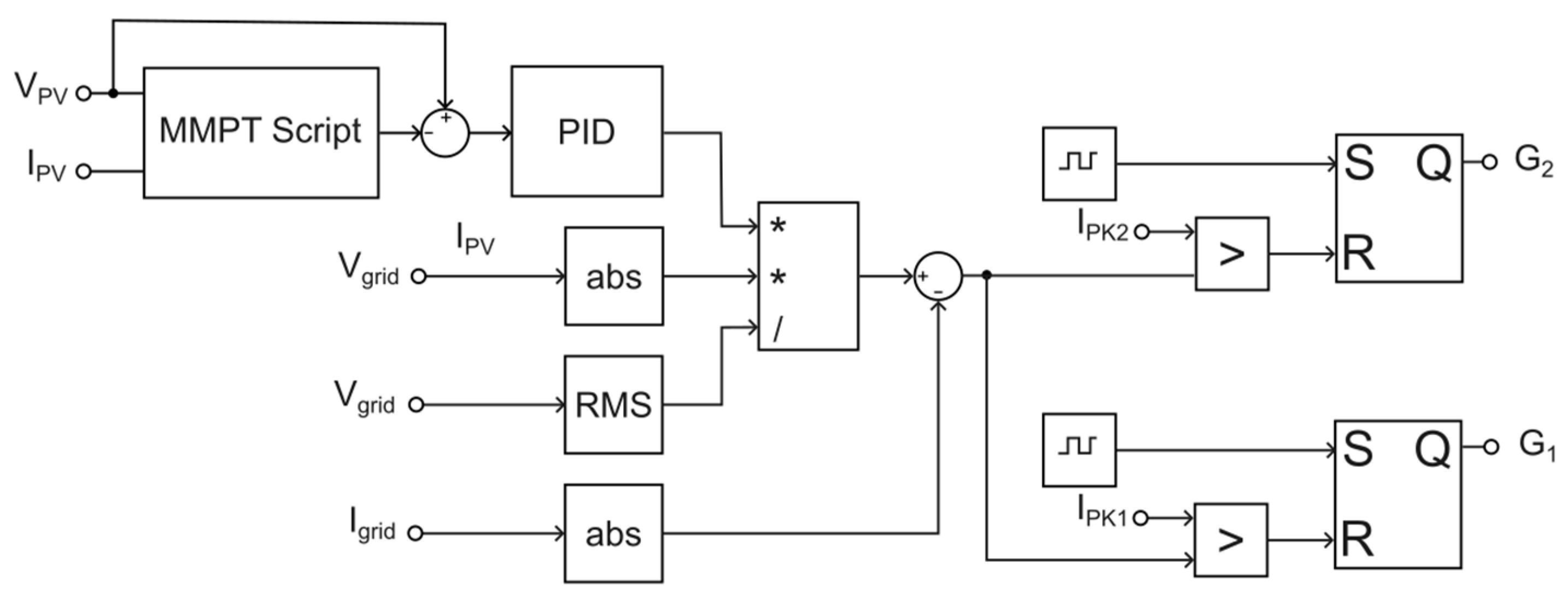
The complete control scheme is shown in Figure 4. Maximum Power Point Tracking (MPPT) is implemented on the PV side. The MPPT block is based on a perturb-and-observe (P&O) algorithm with adaptive step size and protection features, as described in above. It estimates the optimum PV operating point and can output either a voltage reference, a current reference, or a power reference depending on the chosen control mode. In the configuration used here, the voltage reference is applied, which is compared to the measured PV terminal voltage to generate the error signal. This flexibility is valuable, as it allows the same MPPT implementation to be reused in different converter topologies and control architectures.
Figure 4.
Control block diagram.
The error between the reference and measured PV voltage is processed by a PID regulator, which provides dynamic adjustment to drive the PV toward its maximum power point under varying irradiance and temperature. The PID output represents the desired current injection into the grid.
Grid synchronization is handled by a simplified normalization method. Instead of employing a phase-locked loop (PLL), which would be necessary in practical systems subject to grid distortion or frequency drift, the control multiplies the regulator output by the absolute instantaneous grid voltage and divides by the RMS grid voltage. For an ideal sinusoidal grid, as assumed in this study, this guarantees a current reference that is correctly in phase and scaled to the grid voltage without introducing additional control states.
The resulting reference is then compared with the absolute instantaneous grid current. The error feeds into a peak current control loop, which operates at the switching frequency. In each cycle, the current is monitored and compared against the reference; once the threshold is reached, the comparator–RS latch combination terminates the gate pulse. This ensures that the converter injects current into the grid with controlled peak amplitude, maintaining sinusoidal shape while following the MPPT-derived reference.
This layered approach: (1) MPPT for PV optimization, (2) PID for voltage tracking, (3) simplified grid synchronization for phase alignment, and (4) peak current control for fast current regulation—provides both accuracy and computational simplicity. It reflects the goals of the overall model: to retain sufficient fidelity for loss and efficiency estimation while avoiding unnecessary complexity that would slow down large-scale parametric studies.
2.2. Data Extraction
To complement the ideal-switch and simplified magnetic models described in Section 2.1, a set of dedicated data-extraction blocks was developed to estimate the main loss components of the microinverter. These blocks operate in parallel with the simulation, processing measured waveforms such as device currents, voltages, gate signals, and magnetic flux density. The approach allows losses to be reconstructed without introducing parasitics or detailed switching dynamics into the main circuit, thus preserving the numerical efficiency of the model.
Four categories of losses are considered: magnetic core losses, main-switch semiconductor losses, secondary diode losses, and other resistive losses such as copper winding losses and conduction in the low-frequency unfolder switches. For the first three categories, custom C-script blocks implement cycle-synchronous or averaged calculations based on established loss models. The fourth category is estimated analytically using RMS currents and known resistances. Together, these calculations provide a complete breakdown of the losses in the converter and enable accurate estimation of overall efficiency.
2.2.1. Core Losses
Core losses are evaluated from the instantaneous flux density waveform in the transformer. The waveform is obtained from the magnetizing current and geometry of the core, as described in Section 2. A dedicated block processes this signal to reconstruct the losses without adding parasitics into the main simulation.
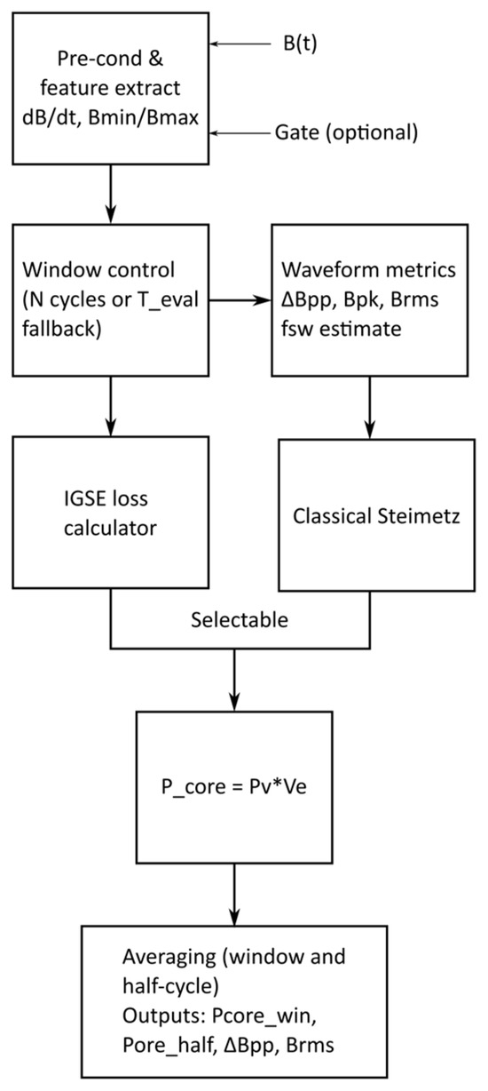
The implementation is shown in Figure 5. The block receives the flux density waveform and, optionally, the gate signal of the main switch. Pre-processing extracts , , and , which are used to determine waveform parameters such as the peak-to-peak excursion , the peak flux , and the RMS flux . A windowing stage groups samples either over a fixed number of switching cycles or a predefined evaluation interval .
Figure 5.
Core-loss estimator block diagram.
Two alternative loss models are available:
Improved Generalized Steinmetz Equation (iGSE).
For an arbitrary waveform segment with flux swing over a time interval , the instantaneous power density is given by (1)
where , , and are material-dependent coefficients. The window-averaged volumetric loss is then
where is the window length.
Classical Steinmetz Equation (CSE).
For sinusoidal approximation, the cycle-averaged loss density can be computed as
where is the switching frequency, the peak flux density, and material coefficients.
The volumetric loss density is multiplied by the effective core volume to obtain the total loss:
Finally, the block performs averaging both over the selected window and over half a grid cycle, producing outputs: window-averaged core loss , half-cycle average , and diagnostics , .
This method captures the combined effect of high-frequency switching and low-frequency modulation from the grid current. By keeping the clamp and other resonant elements out of the main circuit, the simulation remains computationally light while the loss block still accounts for the magnetic stress realistically.
2.2.2. Main-Switch Losses
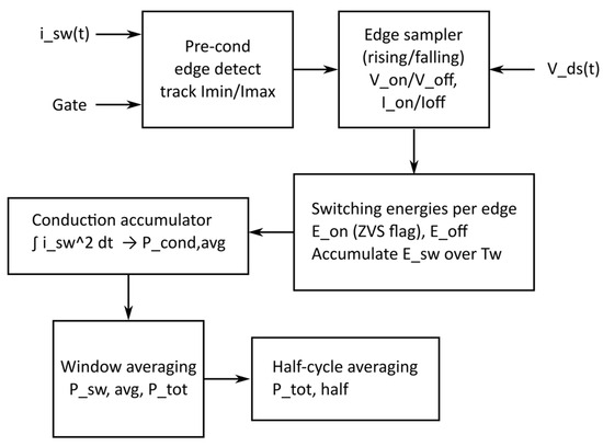
The losses in the main MOSFET switches are divided into conduction losses and switching losses. Since the converter is modelled with ideal switches, these losses are not represented in the circuit waveforms and must be reconstructed by a dedicated estimator. The structure of the estimator is shown in Figure 6.
Figure 6.
Main switch estimator block diagram.
The block receives the switch current waveform , the gate signal, and optionally the drain–source voltage . A pre-conditioning stage detects switching edges and tracks the minimum and maximum current within each conduction interval. At every turn-on and turn-off event, the current and voltage are sampled to form the basis for switching-loss estimation.
Conduction losses.
While the switch is on, conduction losses are determined by the RMS current and the effective on-state resistance :
where is the evaluation window.
Switching losses.
At each transition, the energy is approximated as
where and are the sampled current and voltage at the instant of switching, and are effective switching times, set as tunable parameters. If the ZVS flag is active, is forced to zero. The average switching power over a window is
Total losses.
The total main switch loss is the sum of conduction and switching components:
Finally, the block averages the results both over the switching window and over half a grid cycle, yielding and .
This structure allows the inclusion of realistic switching losses and conduction behaviour while retaining the simplicity of an ideal-switch model. The explicit ZVS flag further enables parametric studies on soft-switching behaviour without introducing resonant dynamics into the main circuit.
2.2.3. Diode Losses
The output rectifier diode conducts whenever the transformer secondary voltage is positive and blocks otherwise. Since ideal devices are used in the circuit model, its losses are estimated in a separate calculation block based on the instantaneous diode current and known device parameters.
Conduction losses.
For a Schottky diode or a fast-recovery diode, conduction losses are given by
where is the forward voltage drop and is the differential resistance. For a SiC Schottky diode, can be neglected and conduction losses are dominated by the constant voltage term.
Reverse-recovery losses.
If a conventional fast diode is modelled, reverse-recovery energy can be included as
with the reverse-recovery charge and the applied reverse voltage. The average contribution over a window is
For SiC Schottky diodes, , and this component is omitted.
Total losses.
The total diode loss is then
averaged over the evaluation window and further averaged over half a grid cycle for efficiency reporting.
2.2.4. Other Losses
Additional loss mechanisms are estimated analytically from RMS currents and known resistances. Copper losses in transformer windings are calculated as
where is the winding current and the DC resistance of the winding.
For the grid unfolder, the switches operate at line frequency, making switching losses negligible. Conduction losses are therefore evaluated as
These contributions are added to the semiconductor and core losses described above to obtain the overall loss balance of the converter.
3. Results
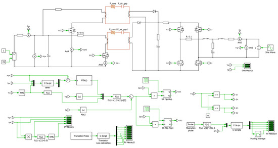
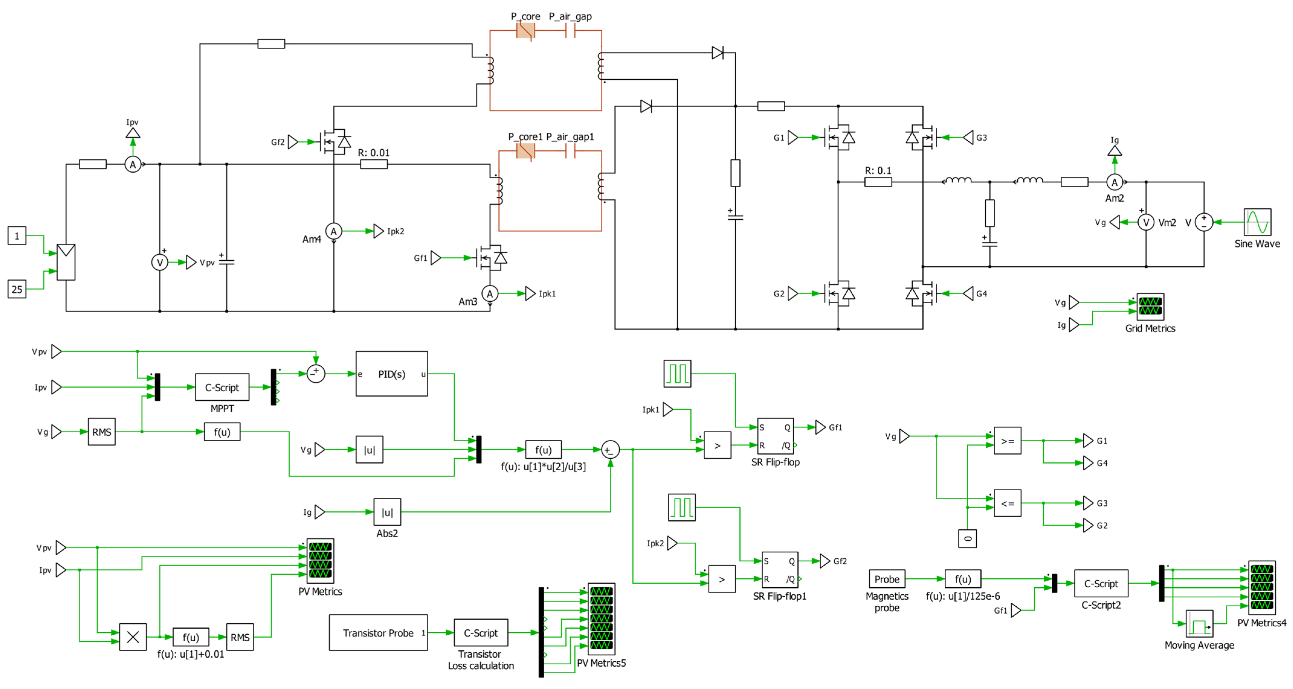
The complete model was implemented and tested in PLECS – V4.7.5, which provides both circuit-level simulation and script-based post-processing capabilities. Figure 7 presents the working block diagram of the system. The upper part of the schematic corresponds to the power stage: the PV source, two interleaved flyback phases, the DC/AC unfolder, and the grid filter. The lower part shows the control and data-extraction subsystems. The MPPT algorithm, implemented in C-script, provides the reference for the PID regulator, which in turn drives the peak-current controllers that generate gate signals for the flyback switches. Additional blocks calculate RMS and averaged grid variables, while dedicated C-script modules process transistor and magnetic probe signals to reconstruct conduction, switching, and core losses as described in Section 2.2.
Figure 7.
Simulation setup diagram.
This integrated implementation enables fast simulation with ideal switches while still capturing realistic efficiency by accounting for major loss mechanisms. In the following subsections, representative simulation results are presented to demonstrate the behaviour of the model under different operating conditions.
3.1. Simulation Setup
For verification, the proposed model was exercised with parameters corresponding to a representative PV microinverter stage. Table 1 summarizes the main component values and device characteristics used. The PV source was set to match a 250 W commercial module, while semiconductor and magnetic parameters were taken from datasheet values or estimated from the physical design.
Table 1.
Verification setup parameters.
3.2. Control and MPPT Operation
To confirm correct operation of the control system, two dynamic cases were simulated.
Irradiance variation.
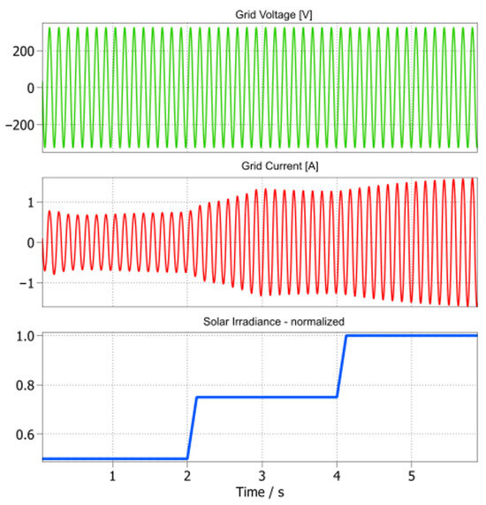
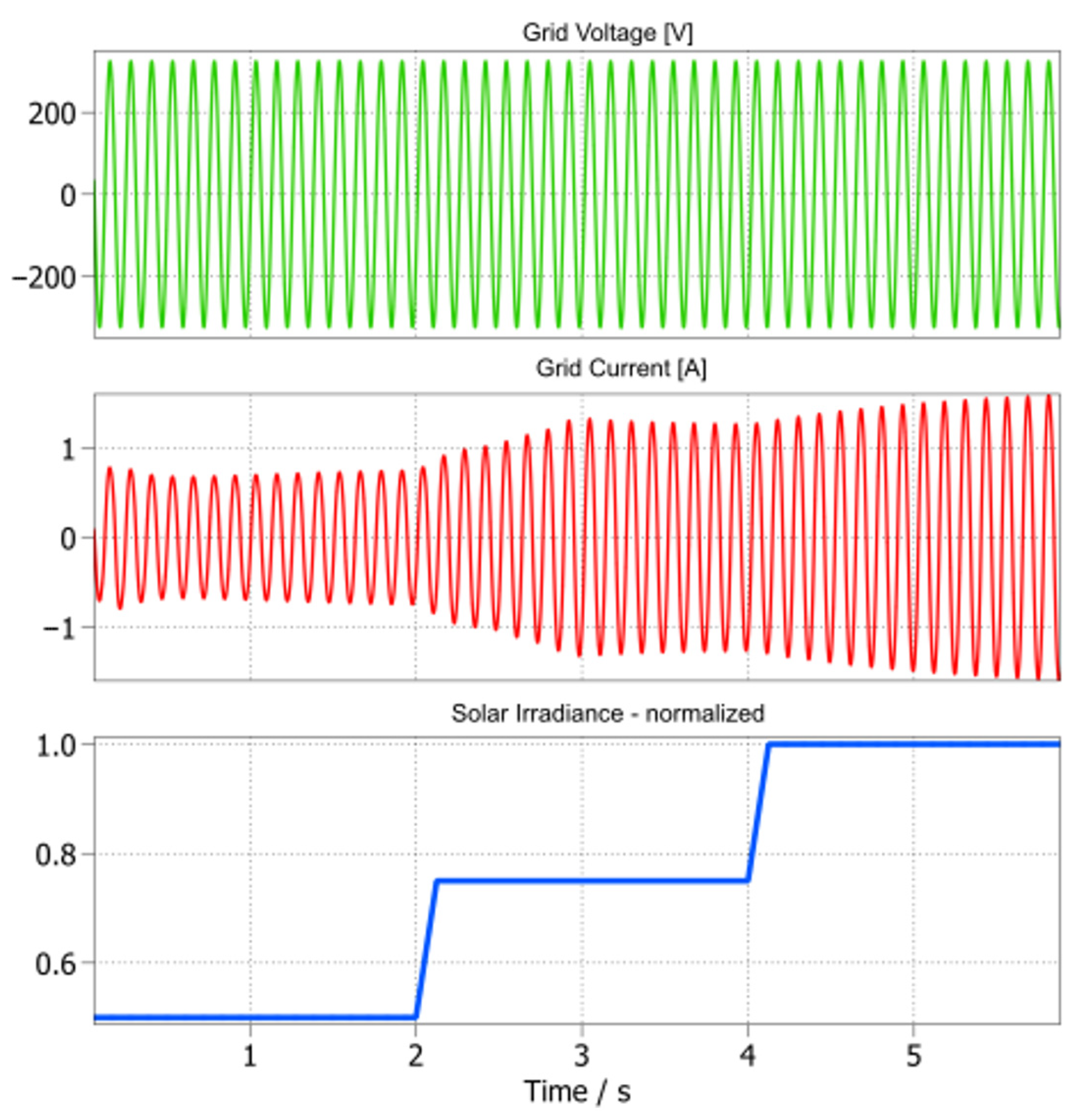
Figure 8 shows the response of the model when solar irradiance is stepped from 0.5 to 0.75 and finally to 1.0 p.u. The PV module power increases accordingly, and the MPPT algorithm adjusts the operating point so that the grid current amplitude tracks the available PV power. The grid voltage remains sinusoidal and unchanged, while the injected current stabilizes quickly after each step, demonstrating that the controller maintains maximum power point tracking under varying input conditions.
Figure 8.
Response of the control system to irradiance variation.
Grid voltage variation.
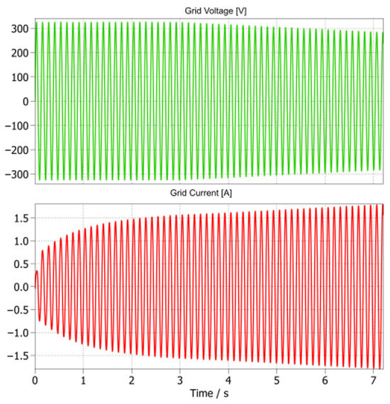
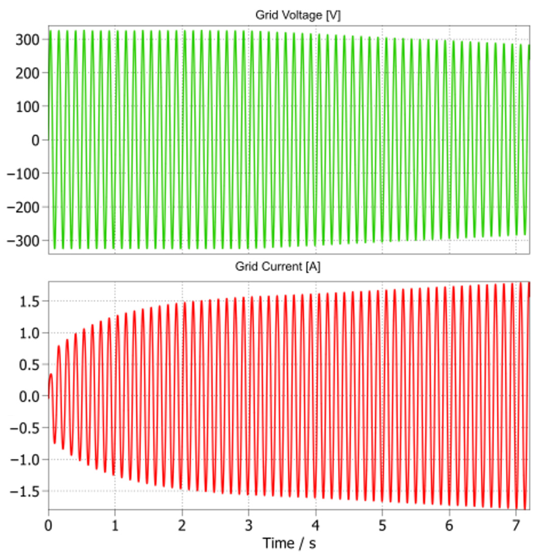
Figure 9 illustrates the case where the grid RMS voltage is decreased from 230 V to 200 V. To maintain the same power injection at the maximum power point, the algorithm automatically increases the current amplitude. The PV voltage and current remain at their MPP values, confirming that the control strategy decouples PV operation from grid variations while still preserving stable current injection.
Figure 9.
Response of the control system to grid voltage variation.
These results highlight that the simplified control structure, combining the MPPT block, PID regulation, and peak current control, is sufficient to capture the essential dynamics of current-source microinverters in the simulation model.
3.3. Loss Analysis
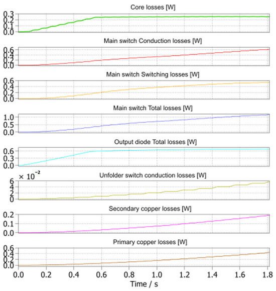
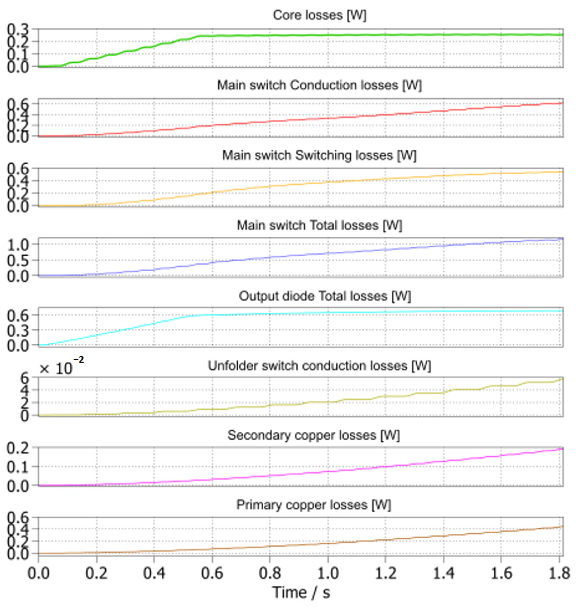
Figure 10 presents the estimated loss distribution of the converter under 0.75 p.u. solar irradiance, corresponding to an output power of approximately 187 W. The results are shown per component.
Figure 10.
Loss breakdown of the proposed model at 0.75 p.u. irradiance.
The dominant contributions are associated with the main switches, which account for roughly 44% of the total losses. Conduction and switching losses are nearly balanced, reflecting the selected device characteristics at 200 kHz. The output diode also contributes significantly, with about 0.6 W per phase, while the magnetic core loss remains moderate at approximately 0.25 W per phase. Copper losses in the primary and secondary windings sum to around 0.7 W per phase. The unfolder bridge, operating at grid frequency, adds only a negligible conduction component.
The total calculated loss at this operating point is about 5.6 W, which corresponds to an overall efficiency of 97.1%. This value is consistent with reported efficiencies of commercial microinverters, confirming that the proposed simplified modelling approach provides realistic results while keeping simulation complexity low.
4. Conclusions
This paper presented a hybrid modelling framework for fast loss estimation in current-source microinverters. The approach combines idealized power stage models with dedicated loss-calculation blocks for semiconductors and magnetics, allowing detailed efficiency assessment without the computational burden of device-level switching simulation. The proposed structure was demonstrated with an interleaved active-clamp flyback converter, but its modularity enables straightforward adaptation to other current-source topologies.
The results confirm that the simplified model can reproduce realistic converter behaviour. The MPPT and control system correctly maintained operation at the maximum power point under varying irradiance and grid voltage, and the estimated efficiency of 97.1% at 0.75 p.u. irradiance aligns with reported performance of commercial microinverters. The loss breakdown further highlights the relative contributions of conduction, switching, and magnetic losses, supporting informed design trade-offs.
The main limitation of the present model is that parasitic dynamics of the clamp circuit and transformer leakage are abstracted into parameters, which may limit accuracy in conditions where resonant transitions dominate. Nevertheless, the framework provides a useful balance of speed and fidelity for parametric studies and early-stage design.
Author Contributions
Conceptualization, A.M. and K.S.; methodology, A.M. and K.S.; software, A.M.; validation, A.M.; formal analysis, A.M. and K.S.; investigation, A.M. and K.S.; resources, A.M.; data curation, K.S.; writing—original draft preparation, A.M. and K.S.; writing—review and editing, A.M.; visualization, K.S.; supervision, A.M.; project administration, A.M. All authors have read and agreed to the published version of the manuscript.
Funding
This research was funded by the National Scientific Programme “Young Scientists and Postdoctoral Fellows”—2.
Institutional Review Board Statement
Not applicable.
Informed Consent Statement
Not applicable.
Data Availability Statement
Data is contained within the article.
Conflicts of Interest
The authors declare no conflict of interest.
Abbreviations
The following abbreviations are used in this manuscript:
| AC | Alternating Current |
| CS | Current Source |
| CSE | Classical Steinmetz Equation |
| DC | Direct Current |
| H-bridge | Full-bridge inverter stage (used for grid unfolder) |
| iGSE | Improved Generalized Steinmetz Equation |
| LUT | Lookup Table |
| MPP | Maximum Power Point |
| MPPT | Maximum Power Point Tracking |
| MOSFET | Metal–Oxide–Semiconductor Field-Effect Transistor |
| PID | Proportional–Integral–Derivative |
| PLL | Phase-Locked Loop |
| PLECS | Piecewise Linear Electrical Circuit Simulation |
| PV | Photovoltaic |
| RMS | Root Mean Square |
| SiC | Silicon Carbide |
| ZVS | Zero-Voltage Switching |
References
- International Renewable Energy Agency (IRENA). World Energy Transitions Outlook; IRENA: Masdar City, United Arab Emirates, 2023. [Google Scholar]
- International Energy Agency (IEA). World Energy Outlook; IEA: Paris, France, 2022. [Google Scholar]
- REN21. Renewables 2023 Global Status Report (Energy Supply). Available online: https://www.ren21.net/gsr-2023/ (accessed on 16 January 2026).
- Zhang, Z.; He, X.-F.; Liu, Y.-F. An Optimal Control Method for Photovoltaic Grid-Tied-Interleaved Flyback Microinverters to Achieve High Efficiency in Wide Load Range. IEEE Trans. Power Electron. 2013, 28, 5074–5087. [Google Scholar] [CrossRef] [Scilit]
- Rojas, D.; Muñoz, J.; Rivera, M.; Rohten, J. Review of Control Techniques in Microinverters. Sensors 2021, 21, 6486. [Google Scholar] [CrossRef] [Scilit] [PubMed]
- Buzzio, C.; Poloni, Y.S.; Oggier, G.G.; Garcia, G.O. A current-source DC-AC converter and control strategy for grid-connected PV applications. Int. J. Electr. Power Energy Syst. 2023, 154, 109399. [Google Scholar] [CrossRef] [Scilit]
- Marignetti, F.; Di Stefano, R.L.; Rubino, G.; Giacomobono, R. Current Source Inverter (CSI) Power Converters in Photovoltaic Systems: A Comprehensive Review of Performance, Control, and Integration. Energies 2023, 16, 7319. [Google Scholar] [CrossRef] [Scilit]
- Edwin, F.F.; Xiao, W.; Khadkikar, V. Dynamic Modeling and Control of Interleaved Flyback Module-Integrated Converter for PV Power Applications. IEEE Trans. Ind. Electron. 2014, 61, 1377–1388. [Google Scholar] [CrossRef] [Scilit]
- Hasan, R.; Mekhilef, S.; Nakaoka, M.; Nishida, K. Soft-switching active-clamp flyback microinverter for PV applications. In Proceedings of the 2016 IEEE 2nd Annual Southern Power Electronics Conference (SPEC), Auckland, New Zealand, 4–7 December 2016; pp. 1–6. [Google Scholar] [CrossRef] [Scilit]
- Kjaer, S.B.; Pedersen, J.K.; Blaabjerg, F. A review of single-phase grid-connected inverters for photovoltaic modules. IEEE Trans. Ind. Appl. 2005, 41, 1292–1306. [Google Scholar] [CrossRef] [Scilit]
- Cordeiro, A.; Chaves, M.; Gâmboa, P.; Barata, F.; Fonte, P.; Lopes, H.; Pires, V.F.; Foito, D.; Amaral, T.G.; Martins, J.F. Automated Solar PV Simulation System Supported by DC–DC Power Converters. Designs 2023, 7, 36. [Google Scholar] [CrossRef] [Scilit]
- Marinov, A.; Solenkov, K. Algorithm for Data Extraction from Photovoltaic Module Technical Documentation. In Proceedings of the 2025 19th Conference on Electrical Machines, Drives and Power Systems (ELMA), Sofia, Bulgaria, 19–21 June 2025; pp. 1–5. [Google Scholar] [CrossRef] [Scilit]

Disclaimer/Publisher’s Note: The statements, opinions and data contained in all publications are solely those of the individual author(s) and contributor(s) and not of MDPI and/or the editor(s). MDPI and/or the editor(s) disclaim responsibility for any injury to people or property resulting from any ideas, methods, instructions or products referred to in the content. |
© 2026 by the authors. Licensee MDPI, Basel, Switzerland. This article is an open access article distributed under the terms and conditions of the Creative Commons Attribution (CC BY) license.