


Abstract
The decarbonization of hospitals located in remote regions with water stress requires a power source that is both reliable and cost-effective. The use of a green hydrogen energy system is proposed for use as the power source for the medical sector located in Ouarzazate, Morocco. The system utilizes photovoltaic panels to power proton exchange membrane (PEM) electrolyzers, which generate hydrogen fuel that is stored in a pipeline to the hospital site where it can be utilized in a fuel cell. A model was created in MATLAB/Simulink R2023a that considered the backward-propagation algorithm to size each of the components of the hydrogen energy system, which was optimized using the particle swarm optimization algorithm. The sizing results of the model indicated that a 924 kW electrolyzer, a 217 kW fuel cell, a 21.5 kW compressor, a 30 mm diameter pipeline, and a 7400 m2 area for the photovoltaic panels are required to supply 161 kg of hydrogen per day to the hospital. The hydrogen fuel system will meet the demand of the hospital for 159 kg of hydrogen per day with a zero loss of load at the deterministic design point, in both the representative day and five-day cloudy-period stress test horizons; a full-physics Monte Carlo uncertainty analysis (N = 10,000 draws) further shows that this reliability outcome is not robust to combined ±20% uncertainty in electrolyzer efficiency and component unit costs, with zero loss of load maintained in 62.8% of draws. The installation cost of the hydrogen fuel system is approximately 8.21 M EUR. Furthermore, because the hydrogen fuel is stored upstream from the hospital, the flow rate of hydrogen fuel that passes through the pipeline is less than if it were stored downstream from the hospital. Finally, the levelized cost of hydrogen fuel of the system is approximately 13.67 EUR/kg, which shows limited sensitivity to the considered variations in solar irradiance. Thus, this hydrogen fuel system methodology can be applied to other types of critical loads, especially those critical loads within hospitals, in regions with high solar potential.
1. Introduction
Ensuring that the hospitals located in remote regions of the world are provided with a continuous supply of power is essential for providing critical healthcare to the residents of those regions. Morocco is a country that is abundant with solar resources, as well as has developed plans for the incorporation of hydrogen-based technologies into critical infrastructures within the country. Despite the advancements that have been made in the production of renewable hydrogen fuel as well as its integration into infrastructure and systems that utilize that fuel, investigations have been insufficient in relation to the potential for incorporating hydrogen energy systems into hospitals [1,2,3,4,5,6,7,8,9,10,11,12,13,14,15,16]. Most of the studies that have been performed regarding hydrogen energy systems have determined the components of those systems according to the supply of hydrogen to those systems. This consideration of the components of systems according to the hydrogen supply to those systems has ensured the maximization of the available renewable energy resources from those systems but has not ensured that the components of those systems will be of an optimal size to provide power to the critical hospitals. Additionally, many of the studies that have been performed on the topic of hydrogen energy systems have considered the transport of the hydrogen fuel to be a less important step than those related to determining the components of the hydrogen energy systems and the fuel that is supplied to those systems, leading to the costly and inefficient components of those systems within the hospitals in which they are installed [17,18,19,20,21].
Although there are numerous published research and development efforts regarding the production of hydrogen fuel through PEM electrolysis, the transport of that hydrogen fuel, and the techno-economic analysis of these processes, there are few studies that have attempted to create a general design framework for hydrogen fuel systems that considers the aspects of reliability for applications like supplying a hospital with hydrogen energy [22,23,24,25,26,27,28,29,30,31,32,33,34,35,36,37].
In an effort to overcome these challenges, a method of determining the size of each component of the PV–hydrogen energy system that can be utilized to supply the hospital in Ouarzazate, Morocco will be utilized. Unlike the common methods of supplying the demand of the load-driven methods for determining the size of each component of the hydrogen energy systems, each aspect of the hydrogen energy system will be sized in a way that ensures that each aspect of the system is sized according to the other aspects of the system that follow the hydrogen energy system components in their function.
The method that is to be utilized within the proposed research article includes the integration of electrochemical, hydraulic, thermodynamic and economic models within the MATLAB/Simulink R2023a environment. Furthermore, a Particle Swarm Optimization (PSO) algorithm will be utilized to determine the configuration of the hydrogen system that minimizes the life cycle cost of the system over a 25-year period [17,18,19,20,21].
Unlike previous studies that have utilized either individual components of the hydrogen system or have used more conventional methodologies for producing the hydrogen fuel, the components that will be integrated into the proposed method include the photovoltaic system, the PEM electrolyzer, the hydrogen compressor, the hydrogen storage system, the hydrogen transportation system, the hydrogen regulator, and the PEM fuel cell. Each of these components will be optimized to determine the best design for the hydrogen production and reconversion to electricity process.
Each of the three aforementioned technologies is well established within the technical literature. The novelty of this document, however, is the application of these concepts to the sizing of hydrogen systems with reliability constraints (LOLP = 0) and hospital-scale hydrogen systems requirements, a concept that has not been described within the technical literature regarding hydrogen systems. Thus, the main contributions of this document are as follows:
The propagation of reliability and hydraulic system constraints (such as the diameter of the pipeline, the velocity of the fluid within the pipeline, and the pressure of that fluid) within a demand-driven, backward-propagation sizing methodology for hydrogen systems an approach that has previously been applied to systems related to battery storage systems to the hydrogen pipeline system.
A coupled multiphysics model built in MATLAB/Simulink that includes all of the pertinent components of the hydrogen energy system (PV, PEM electrolysis, hydrogen compression, storage, hydrogen transport through pipeline, pressure regulation, PEM fuel cell).
An optimization framework based on particle swarm optimization to minimize the techno-economic objective function of the system while satisfying various constraints.
Independent validation of each of the subsystems of the hydrogen energy system prior to evaluating the performance of the coupled system.
Comprehensive sensitivity and probabilistic uncertainty analyses of the methodology proposed in this paper.
The remainder of the paper is organized as follows. Section 2 reviews the literature regarding PV-H2 systems, hydrogen transportation through pipelines, and techno-economic optimization methods. Section 3 describes the proposed method for investigating the hydrogen energy system. Section 4 details the mathematical models of each of the components of the hydrogen energy system. Section 5 details the methods that were utilized to optimize the hydrogen energy system. Section 6 describes the case study that was performed as a means of evaluating the proposed methodology. Section 7 presents the results of the validation of the model and simulations performed with the model. Section 8 discusses the results of the sensitivity and uncertainty analyses of the system performed in this paper. Finally, Section 9 presents the main findings of this paper and suggests future research directions.
2. Literature Review
2.1. PV–Hydrogen Hybrid Energy Systems
While the literature on PV- systems is quite developed, most of the studies make simplifications regarding the coupling between the different components of the system. More recent studies on the operation of electrolyzers have demonstrated that the main challenge in the operation of electrolyzers is not feasibility, but rather the management of the variables related to intermittency and the degradation of the electrolyzer, as well as the coupling between the different dynamic variables of the system. Ulleberg [22] developed one of the foundational models for dynamic simulations of alkaline electrolyzers; Ursúa et al. [23] performed a review of the state of the art and trends in water electrolysis technologies; and Carmo et al. [24] performed a review of the technology of PEM water electrolysis. The same trend of focusing upon the characterization of the technology while ignoring the coupling between dynamic system variables is also seen in the techno-economic analyses of green hydrogen production plants that utilize these models for electrolyzers [22,23,24]. While the dynamic models have helped to establish the theoretical basis for hydrogen production using renewable energy, the models are generally limited to those that do not consider the interaction between the PV systems and the electrolyzers. Almpantis et al. [25] proposed an optimization framework for PV-PEM electrolyzer systems that used machine learning methods to approximate the costs of various system configurations an approach that is closer to optimizing the system as a whole than are the models that have gone before. However, like most of the research that has gone into hydrogen fuel production in the past, these methods are technology oriented in their consideration of the requirements of both electrolyzers and PV systems, and do not consider the impact that the technology of the electrolyzer can have upon the reliability or hydraulic design of the hydrogen delivery system. More recent investigations into the viability of PV–electrolyzer–fuel cell chains have generally confirmed the viability of these systems, but generally only in assessing their efficiency, their energy production, or their feasibility on a small scale. The integration of these systems into hydrogen transport and storage systems has been somewhat limited by their intermittency, their potential for component mismatch, and the lack of modeling of aspects related to the transport of the hydrogen gas. Thus, while there are numerous technologies related to the PV–hydrogen systems that are generally considered to be mature technologies, much of the existing literature related to hydrogen production is either focused upon the various components of these systems, or their reliability as systems as a whole.
2.2. Hydrogen Pipeline Transport
Pipelines are one of the issues regarding hydrogen that is generally ignored by many studies into the production of renewable hydrogen. While the principles of hydrogen transport through pipelines was established in older studies on the topic, subsequent studies have indicated that the models established for those studies were only valid under limited conditions for hydrogen transport. Studies into supply chains for hydrogen have established that the mode of transport for the hydrogen gas is dependent upon a variety of factors, including the distance that the hydrogen must travel, the rate at which the hydrogen must be transported, and the cost of constructing the infrastructure necessary to transport the hydrogen. Authors such as Menon [28] have investigated the hydraulic principles of transporting gases through pipelines. Chaczykowski [29] has investigated the accuracy of different models for transporting gases through a pipeline network. Reuß et al. [30] have established models for the storage of hydrogen gas within a supply chain, and authors such as Hasanli [31] have investigated the degree of conservatisms of a standard pipeline model when applied to the transport of hydrogen gas.
Going beyond the study of the hydraulic properties of hydrogen within individual pipelines, recent studies have begun to determine the optimal design of the hydrogen infrastructure systems required to transport the gas. Studies that have investigated the concept of utilizing natural gas pipelines for hydrogen transport have determined the various issues that can result from such a process. Other studies that have investigated hydrogen transportation networks have found that the route of the hydrogen pipeline can impact the infrastructure requirements and costs of the hydrogen transport system. These studies, however, have mainly considered hydrogen transportation networks on a regional scale. Factors related to the transport of hydrogen within a hospital system, such as the diameter of the transport pipeline, the power required to compress the hydrogen gas, the location in which the hydrogen is to be stored, and the feasibility of the transport of hydrogen at certain pressures, all impact the power that can be supplied to the hospital’s electrical system [28]. This impact of various factors upon the electrical system of a hospital has also been recognized in a study of the layout of the hospital infrastructure as a whole by Fang et al. [32].
In this project, therefore, the hydrogen transport pipeline will be considered as that which is to be determined for the system. The hydraulic properties of the hydrogen that travels within the transport pipeline will have an impact upon the design of the compressors to be utilized within the hydrogen system, the structure of the storage infrastructure for the hydrogen, the feasibility of the transport pressures for the hydrogen within the system, and the overall techno-economic design of the system altogether.
2.3. Techno-Economic Optimization
The techno-economic approach to the optimization of the hydrogen infrastructure is the de facto approach to be utilized in the design of such systems. The PSO algorithm is one of the most common approaches to be utilized in determining the optimal configurations of the hydrogen infrastructure systems from its design variables. Despite numerous alternatives to PSO algorithms existing in the current literature, PSO is still one of the most common techniques in energy and renewable energy systems implementations of PSO algorithms [33,34,35,36].
There are various uses of AI in the context of hydrogen energy systems, though mostly in relation to hydrogen energy management and estimation of the parameters of the system. The methods are, however, mostly simplified in relation to the processes of electrolysis, compression, storage of the hydrogen, movement of the hydrogen through hydrogen pipelines, and the use of fuel cells to convert the hydrogen back into usable energy. Beyond PSO, other methods proposed for general Power-to-Hydrogen system designs include Mixed Integer Linear (or Non-linear) Programming (MILP/MINLP) methods, which find the optimal solution to convex or linear problems but have poor scalability to the non-convex problems that are common in hydrogen systems; dynamic programming methods, which are effective optimization techniques for problems of relatively small dimension but which suffer from the curse of dimensionality; Model Predictive Control (MPC) methods, which are the preferred method of controlling the operation of the power-to-hydrogen systems in operation but which are not applicable to the sizing of those systems; and other metaheuristics like genetic algorithms, simulated annealing, and differential evolution algorithms, which are similar to PSO in that they can be utilized with non-convex problems. PSO was chosen among these alternatives due to its relative simplicity in relation to the other algorithms, its existing use in similar problems, and its compatibility with the MATLAB/Simulink model. Furthermore, as covered in Section 6.4, PSO was chosen as one of the methods that has been successful in solving these types of problems. Thus, PSO was an appropriate method for solving the presented problem [33,34,35,36,37].
2.4. Research Gap and Positioning
Within the existing literature regarding renewable technologies, there has been some development in various components of the technology. However, the existing literature is fragmented and often limited to studies that are dedicated to specific components of the H2 technology. For instance, Ulleberg published a study regarding electrolyzers alone [22], Ursúa et al. published a study regarding electrolyzers alone [23], Menon published a study regarding transportation via pipelines alone [28], and Larminie and Dicks published a study regarding fuel cells alone [37]. However, the limited number of studies that have been published about each of the components of the technology (PV, PEM electrolyzer, compression, transportation, storage, fuel cells) indicates a research gap in the publication of studies that consider the potential for integrating these components into a study dedicated to the technology [22,23,24,25,26,27,28,29,30,31,32,33,34,35,36,37].
The concept of sizing each of the components of the technology according to the demand for that has been employed for technologies like batteries and microgrids. In each of these technologies, the size of the energy storage technology is determined according to the load that is to be supplied to those technologies, and the determination of that size ends with that energy storage technology alone, such as in the sizing studies of the hydrogen pipelines and infrastructure described above [28,32], in the MINLP-based hydrogen network topology optimization of Jamali et al. [38], and in the pipeline–road coordinated hydrogen transportation scheduling of Tan et al. [39]. For hydrogen technologies, however, the diameter of the hydrogen pipeline, the size of the pumps that will be used to compress the hydrogen gas to the necessary levels for transportation, and the number of stages at which that hydrogen will be compressed is determined after the determination of the size of the hydrogen production and storage technologies, as well [28,32,38,39]. Thus, while the hydrogen system that is proposed within this study may employ these sizing concepts as a means of determining the sizes of the hydrogen production and storage technologies to be employed within the hydrogen supply system, the contribution of this study is to extend these sizing concepts to the determination of the diameter of the hydrogen pipeline that is to transport the hydrogen from the production location to the end use location, and the size of the hydrogen compressors that are to enable the transport of the hydrogen to those end use locations, while maintaining a LOLP of zero for the hydrogen supply system a combination of factors that have not previously been attempted to apply to the field of hydrogen supply technologies, especially to those technologies that are to supply hydrogen to critical locations within the nation.
Given the abundance of renewable resources in the nation, the integration of green hydrogen into its critical-load applications is lacking. The present study aims to fill such a gap by determining the amount of each component of a green hydrogen system required to supply energy to a hospital in Ouarzazate. The integration of several models into a single optimization framework allows for the assessment of the technical and economic feasibility of the system.
While several previous studies considered the incorporation of hydrogen transport or multiphysics simulations into PV-PEM systems, no studies have considered the optimization of such a system with respect to the reliability of hydrogen delivery at a critical load (LOLP = 0) for a specific application.
3. System Architecture and Backward-Propagation Methodology
3.1. System Description
The proposed integrated system consists of eight main subsystems: PV array (located at NOOR I), PEM electrolyzer, hydrogen compressor, hydrogen storage tank, stainless-steel 316 L pipeline (19.7 km long), pressure regulation stage, PEM fuel cell, and the hospital electrical loads. The solar irradiance that falls upon the PV array will be converted into electrical energy. The PEM electrolyzer will use this electrical energy to produce hydrogen and oxygen. The hydrogen will be compressed by the hydrogen compressor and stored in the storage tank. The hydrogen will be transported through the pipeline to the PEM fuel cell where it will be expanded to the required pressure for the fuel cell and then fed into the fuel cell. The hydrogen in the fuel cell will be converted into electricity that will power the medical buildings. The oxygen will be purified and used for medical applications.
Unlike most of the existing renewable hydrogen systems, all of the components of the proposed system are physically coupled together in a way that allows for each of the components of the system to be optimized in relation to the others in order to achieve the best possible performance of the system overall.
As mentioned previously, because the main use of the hydrogen fuel cell system is the supply of electricity to the hospital, it is necessary to justify the use of the process of converting the electrical energy to hydrogen fuel and then back to electrical energy. The reasons for which these types of conversions are performed include the need to supply the hospital with a renewable supply of energy that is available even after dark, or during periods of cloudy weather, which necessitates the use of energy storage technologies. Furthermore, because the efficiency of converting electricity to hydrogen fuel and back to electricity is less than the efficiency of the battery-based storage of electrical energy, the use of a PV and battery system will be more cost effective than a system that relies upon the production and storage of hydrogen fuel. However, the scaling of battery storage is less favorable than hydrogen storage for applications that require multi-day autonomy (3–5 days). Battery storage capital costs scale linearly with the amount of stored energy, while the cost of hydrogen storage is dominated by the relatively cheap storage vessel needed to store the hydrogen, once the cost of the electrolyzer and fuel cell are accounted for. While a PV–battery–diesel system would be reliable and cost effective relative to the system proposed in this work, it would reintroduce the considerations of dependence upon a fossil fuel, the logistics of transporting that fuel to the remote region, and the emissions of pollutants that negatively affect the health of patients at the healthcare facility all of which were the considerations that motivated the investigation of the fully renewable pathway for power supply to the facility. A PV–battery–hydrogen system would likely be the best alternative to the hydrogen system proposed in this work, motivating investigation of such a system as part of future work. However, a thorough cost comparison of each of these system architectures (PV, PV–battery, PV–battery–diesel, PV–battery–hydrogen, and the all-hydrogen system proposed in this work) is beyond the scope of this investigation. Such a cost comparison is a direction for future research, therefore. Table 1. Cost and performance comparison for various hydrogen-based power system architectures.
Table 1.
Comparison of key methodological features across representative studies.
System LCOE (EUR/kWh) LCOH (EUR/kg H2) Notes
- PV only with diesel backup 0.15–0.25 Fuel dependent cost; lowest CAPEX; requires fuel deliveries for autonomy.
- PV with battery (Li-ion, 1-day autonomy) 0.20–0.35—Battery-dependent cost; requires battery for autonomy.
- PV–battery–diesel 0.12–0.20 Lowest cost of the alternatives Includes emissions and fuel delivery costs.
- PV–battery–hydrogen 0.25–0.40—Published literature data is limited regarding hospital power applications.
All-hydrogen system 0.82 13.67 13.67 EUR/kg H2 median; 12.62–14.69 EUR/kg H2 10th–90th percentile; delivered-electricity cost accounts for the 33.33 kWh/kg (LHV) hydrogen energy content and the 50% fuel cell conversion efficiency (Equation (46)); costs for this technology are higher than the other systems indicated; however, the primary motivation to utilize hydrogen fuel cells (instead of conventional systems) is due to the ability of hydrogen systems to provide multi-day autonomy for energy systems off-grid, with zero on-site emissions; thus, performing a dedicated techno-economic analysis on this hydrogen system specific to the hospital and site in question would be necessary to confirm these cost figures (at order-of-magnitude).
Table 1 indicates that the all-hydrogen system is the most expensive of the alternatives relative to the unit costs of energy delivered (although it remains competitive in relation to other alternatives regarding other system performance and environmental metrics, such as autonomy, emissions, fuel diversification, etc.). Thus, while the motivation to employ hydrogen fuel cells for the delivery of electricity to the hospital off-grid from the power grid is based upon the benefits of hydrogen fuels (rather than their cost), a dedicated techno-economic analysis of the all-hydrogen system relative to the hospital site would be necessary to confirm these cost figures to the precision indicated in the table.
The energy conversion of the proposed system can be described as:
where G is the solar irradiance, is the PV area, and the remaining terms are the energy states of the system in each of the components.
3.2. Backward-Propagation Sizing Methodology
Following the concept of backward propagation of the demand for electricity within the hospital for sizing, the load from the hospital is considered to be the terminal boundary condition for the energy system. The size of each component of the system is sized to ensure that the demand for electrical or hydrogen power from the upper components of the system is fully met by the lower component of the system. Thus, the sizing of the components occurs from the critical load to the system backwards, rather than from the requirement for renewable energy production within the system.
The demand for the medical sector is 2500 kWh of energy per day, with 1200 kWh from the hospital itself, 1000 kWh from two clinics, and the remainder (300 kWh) for the dialysis center. This daily energy total and its diurnal shape are derived from real hourly/sub-hourly smart-meter consumption data measured at the Centre Hospitalier Provincial Sidi Hssain Bennaceur (Ouarzazate, Morocco) and its associated primary-care clinics over a full year (exact measurement period withheld for facility confidentiality), rather than a synthetic or literature-based construction; the 2500 kWh/day figure and the 104/208 kW average/peak values correspond to a representative day extracted from this annual measured dataset, resampled to 60 s resolution for the time domain simulation. The corresponding solar resource remains a synthetic clear sky irradiance profile for the Ouarzazate site (not a measured or satellite-derived TMY dataset), generated at the same 60 s resolution and used consistently for both the nominal day results of Section 6 and the 5-day cloudy period stress test of Section 7. While the hospital load side of the reliability analysis is therefore grounded in real annual metering data, the present simulation still evaluates only a single representative day (plus the 5-day stress test of Section 7) drawn from that year rather than the full annual load and irradiance time series; extending the chronological simulation to run the complete measured annual load profile against a site-specific TMY solar dataset, to capture the actual seasonal coincidence of low irradiance periods with high demand periods across the year, is identified as a priority extension of this work and is stated as a remaining limitation of the present study. Each of these loads equates to an average power load requirement of 104 kW for the medical sector. The size of the fuel cell is sized to deliver the load of the hospital at each time step in the day ( (t) = (t)), thus ensuring that the probability of loss of load from the fuel cell is zero. The fuel cell, therefore, must have a nominal power of 208 kW to meet the load demand of the hospital.
The corresponding hydrogen demand can be obtained from the fuel cell power requirement as:
Equation (2) yields a hydrogen demand of 152 kg/day for the medical buildings and 10 kg/day for the ambulance fleet for a total demand of 162 kg/day. This initial backward-propagation estimate is subsequently refined once the time-resolved fuel cell simulation and final operating assumptions are applied (Section 6): the corresponding steady-state consumption is 159.1 kg/day, while the PSO-optimized electrolyzer produces 161.4 kg/day, exceeding this consumption and providing the margin discussed in Section 6.1. Such a hydrogen flow can be propagated upstream to determine the necessary size of the compression, storage, pipeline, electrolyzer, and photovoltaic systems.
The hydrogen production, compression, storage, transport, and utilization can be defined through a staging of the system according to the system’s thermodynamics and hydraulic functioning. For instance, PEM electrolyzers operate at around 30 bar of pressure, the hydrogen fuel can be compressed to around 200 bar for storage, the inlet pressure within the hydrogen transport pipeline can be maintained at between 180 and 200 bar, the outlet pressure of the hydrogen pipeline must be at least 150 bar to avoid the need for a hydrogen compressor at the pipeline’s outlet, and the hydrogen must be regulated to a pressure of between 2 and 3 bar prior to its utilization in the fuel cells powering the ambulance fleets.
The pipeline diameter is sized from the Darcy–Weisbach relation for steady state compressible gas flow:
where is the friction factor from the Colebrook–White correlation and the other variables are as explained above. The mass flow rate can be written as:
which describes the gas density and gas velocity in the pipeline between 5 and 10 m/s. The internal diameter of the pipeline is chosen to satisfy both the pressure drop and velocity criteria, making the diameter of the pipeline a design variable, following the sizing methodology of Menon [28] as extended to multi-component hydrogen systems by Fang et al. [32].
The compressor and storage unit are sized according to the chosen pressure staging. For the reference configuration, the compressor will stage the pressure of the hydrogen from 30 bar at the outlet of the electrolyzer to 200 bar at the storage unit inlet. This high-pressure buffer will be sized to provide operational autonomy to the hydrogen system while still remaining within the chosen pressure stage. Furthermore, the use of the centralized storage units upstream of the hospital is employed to reduce the required flow rate of the hydrogen through the delivery pipelines, to reduce the pressure losses within the delivery system, to enhance safety by keeping high pressure equipment away from the hospital campus, and due to the cost and reliability considerations discussed in the pipeline hydraulics [28] and infrastructure layout [32] literature cited above.
Finally, the PEM electrolyzer and PV field are sized to meet the hydrogen production target. The PEM electrolyzer is sized to meet the hydrogen demand of the system. The PEM electrolyzer comprises multiple identical modules to allow for modularity in the system. The PV field size is sized according to the hydrogen production target and solar resource availability. Mass conservation of hydrogen is enforced throughout the system as:
This equation is used as the basis for the optimization framework for the system as described in the following section. Equation (5) assumes steady-state mass conservation across the electrolyzer, compressor, pipeline, regulator, and fuel cell; the hydrogen storage subsystem interposed between the compressor and the pipeline (Section 3.3 and Section 5.2) is explicitly not steady-state, and instead governed by the mass balance ordinary differential equation − , where (t) is the compressor outlet flow (charging) and (t) is the flow drawn toward the pipeline and fuel cell (discharging). The storage tank design capacity is considered within the range of 480–800 kg H2, corresponding approximately to 3–5 days of autonomy. For the selected 800 kg design capacity, the chronological simulation uses an initial inventory of 640 kg H2 and imposes a minimum operating inventory of 24 kg H2 as a hard lower bound; (t) is therefore bounded between this 24 kg operating floor and the 800 kg design capacity (Section 5.2). Equation (5)’s steady-state mass conservation therefore applies instantaneously to every subsystem except storage and applies to storage only in a time averaged sense over a full charge/discharge cycle (i.e., daily (integrated over the cycle equals daily )). The explicit time domain solution of this storage ODE, including a multi-day stress test, is presented in Section 7 and Section 8 (LOLP analysis).
3.3. Storage Topology and Hydraulic Implications
Three different hydrogen storage topologies were evaluated for the system. Scenario 1 (S1) evaluated the hydrogen storage downstream of the hospital but instead distributed the hydrogen for only 8 h per day. Scenario 2 (S2) evaluated the hydrogen storage upstream of the hospital, from which the hydrogen was distributed for 24 h per day. Finally, Scenario 3 (S3) evaluated the hydrogen stored for 12 h per day, which is midway between the other two scenarios.
The main difference between these three scenarios is the mass flow rate of the system. As discussed in scenario two, the longer that the hydrogen is distributed, the lower the mass flow rate of the system. Thus, scenario 1 has three times the mass flow rate of scenario two (due to the distribution for only 8 h per day compared to 24 h per day), and scenario three has twice the mass flow rate of scenario two (due to the 12 h distribution period). Thus, the hydrogen storage topology is both a consideration of the design of the storage components of the hydrogen system, as well as the hydraulic components of that system.
Scenario S2 was chosen to be used as the reference scenario for the remainder of this study. Scenario S2 has the lowest flow rate for the hydrogen, the most favorable pressure drop along the system, and has the best safety considerations for the hospital campus. Thus, Scenario S2 represents the best compromise between each of these considerations, as well as the trade-offs between the costs associated with each of these factors, as established by Zhang et al. [41], Fang et al. [42], and Schofield et al. [43]. Scenario S2 will therefore be used as the basis for the remainder of this study.
4. Mathematical Models
The mathematical models that will be utilized for the I-HES will be formed under the following set of assumptions: that the system is in a state of steady state for the hydrogen transport, that there is negligible leakage of the hydrogen from the system, that the transport of the hydrogen within the hydrogen pipelines is one dimensional, that the composition of the hydrogen within the pipelines is constant, and that the regulation of the pressure within the system is ideal. The fact that hydrogen is a real gas can be accounted for by an engineering hydrogen compressibility (Z) correlation calibrated against NIST reference data (Section 4.4.2), rather than a full Peng–Robinson equation of state, since the working fluid is pure hydrogen and no multi-component mixing rule is required. The equations for the I-HES will be solved according to the methodology introduced in Section 3.
4.1. Photovoltaic System
The PV array output power at time t is modeled by correcting the rated power for solar irradiance and module temperature:
where is the rated power under standard test conditions (1000 W/, 25 °C), G(t) is the irradiance, = −3.7× ° is the temperature coefficient, and = 25 °C. The cell/module temperature (t) is itself computed from ambient temperature and irradiance via the standard Nominal Operating Cell Temperature (NOCT) model, rather than being set equal to ambient temperature: (t) = (t) + [(NOCT − 20)/800] × G(t), with NOCT = 45 °C (typical manufacturer-rated value for crystalline-silicon modules) and G(t) in W/m2. This distinguishes the module operating temperature which can exceed ambient by 20–25 °C at full irradiance and drives the temperature-derating term above from the ambient air temperature used only as an input to this NOCT relation, correcting for the use of ambient rather than module temperature in the electrolyzer power correction. The annual PV energy yield is obtained by time integration of the hourly power profile. The PV subsystem provides the electrical input to the electrolyzer during hydrogen production periods.
4.2. PEM Electrolyzer
PEM electrolysis was selected over alkaline electrolysis for this application despite the latter’s technological maturity and generally lower capital cost. This choice reflects three characteristics of the case study that favor PEM technology: (i) the intermittent, PV-driven power supply requires an electrolyzer capable of rapid load-following and frequent start/stop cycling without the minimum load and degradation penalties associated with alkaline stacks operating below roughly 20–40% of rated capacity; (ii) PEM stacks natively produce hydrogen at higher outlet pressure (here, 30 bar) than atmospheric alkaline units, reducing the compression ratio required upstream of storage; and (iii) the compact footprint of PEM stacks is advantageous for a hospital-adjacent installation with constrained available area. These operational and integration advantages are judged to outweigh the higher capital cost of PEM for the reliability-critical, renewable-coupled application considered here; a full techno-economic comparison between PEM and alkaline electrolysis is left for future work. The PEM electrolyzer converts electrical power into hydrogen via water electrolysis. The single-cell voltage is written as:
where is the reversible voltage and , , and denote the activation, ohmic, and concentration overpotentials, respectively. The electrical power consumed by the stack is:
And the corresponding hydrogen production rate is:
where is the electrolyzer efficiency and is the lower heating value of hydrogen. This equation describes the electrochemical basis of the hydrogen conversion process and its implementation in MATLAB/Simulink. The stack itself is modeled with a first order thermal submodel and a minimum loading constraint to represent warm-up and partial load conditions. The hydrogen production rate from this block is passed to the compression stage.
When the electrolyzer is running at less than its nominal design capacity, the surplus PV electricity can be curtailed or used to increase hydrogen production.
Water Balance
The 1458 L day−1 water figure reported in Section 6.3 was computed from PEM electrolysis stoichiometry alone. A complete water balance for the water-scarce Ouarzazate region must additionally account for the reverse-osmosis (RO) pre-treatment recovery ratio, cooling-water makeup for stack thermal management, and other auxiliary consumption, since the process (feed) water demand exceeds the stoichiometric (reacted) water demand:
where is the reverse osmosis recovery ratio, is the rate at which makeup water is added to the thermal system to remove waste heat, and is the rate at which other process water is consumed (typically for humidification of gases and waste purge gases). The RO process also requires some electrical energy to be operated, which should also be included within the energy balance for the electrolyzer and PV systems once a specification for the RO system is chosen.
Because Ouarzazate is located in a semi-arid and arid climate, water resources are relatively limited within the region. Thus, the availability of water within the region is another assumption of the system that must be verified before the reliability of the system can be generalized. Using an estimated value for the RO recovery ratio of approximately 75% (with recovery ratios typically ranging between 65% and 85%), an additional 10% of the total water requirements for cooling the RO system, and an additional 5% of the total water for auxiliary uses, the total water requirement for the system increases from the stoichiometric requirement of 1458 L day−1 to approximately 2070 L day−1—an increase of 42%. Furthermore, RO systems typically have a specific energy consumption of between 1 and 2 kWh m−3 of treated water. Thus, RO will consume between 2 and 4 kWh day−1 of energy though this is relatively small compared to the estimate of 8000 kWh day−1 of energy that is required for the entire system (calculated in Section 6.3); yet, which should be included within the energy balance of the electrolyzer and PV systems once the RO system is specifically chosen and specified. Such estimated values will be replaced with the actual values of the water source that will be used, the RO system that will be utilized, and the seasonal availability of that water resource.
4.3. Hydrogen Compressor
The compressor stages the hydrogen from the electrolyzer outlet (30 bar) to the storage pressure of 200 bar, as described in Section 6.4. Each stage of compression is adiabatic with a constant per-stage isentropic efficiency. Furthermore, intercooling between stages reduces the temperature of the hydrogen between each stage of the compressor to the same inlet temperature that is used for each stage of the compressor an assumption that is made for simplifying the description of the compressor’s duty as the sum of the per-stage work required to adiabatically compress the hydrogen to each stage’s exit pressure. The electrical power required for each stage of the compressor is given in Equation (10) below. The total power for the compressor, calculated in Section 6.1, Section 6.2, Section 6.3 and Section 6.4, is the expression given in Equation (10) multiplied by the number of stages that are required to reach the storage pressure of 200 bar with each stage having a relatively low and practical pressure ratio (around 3:1 to 4:1 per stage):
where is the gas constant of hydrogen, is the inlet temperature, γ is the specific heat ratio, and is the compressor isentropic efficiency. The use of this expression for each stage of compression, along with the inter-stage cooling described above, allows for the high overall compression ratio from 30 bar to 200 bar to be approximated by an isothermal compression process. The compressed hydrogen is then transferred into the storage and pipeline subsystem.
4.4. Hydrogen Pipeline
4.4.1. Mass Conservation
Under steady operation, and neglecting leakage and line-pack effects, the hydrogen mass flow remains constant along the pipeline:
4.4.2. Hydraulic Formulation
The storage tank is maintained at the selected pressure, and the pipeline inlet pressure is assumed equal to this value. Pressure decreases along the line due to frictional losses. Hydrogen density is evaluated from:
where Z is the compressibility factor obtained from the Peng–Robinson equation of state as a function of pressure and temperature.
The pressure drop is estimated using the Darcy–Weisbach relation:
where f is the friction factor, L is the pipeline length, D is the internal diameter, is the gas density, and v is the mean velocity. The mass flow rate is related to the pipe geometry as:
The friction factor is determined from the Colebrook–White equation from the roughness of the pipe and the Reynolds number. A range of 5 to 10 m/s is used only during the backward-propagation pre-sizing stage of Section 3.2 in order to determine the nominal diameter of the pipe. The diameter is the free variable within the PSO algorithm (constraint (38) below), and the cost minimizing optimum to the PSO algorithm indicates a diameter that results in a lower velocity within the pipeline of 0.184 m/s (Section 6.2). Thus, although the velocity constraint within the PSO algorithm is set to the upper bound of 15 m/s, the actual velocity within the optimized design is both within the turbulent flow constraint and is well below the 5 to 10 m/s nominal range. The diameter of the pipe within the bounds of the PSO algorithm is chosen such that the pressure loss and velocity criteria of the constraints (37)–(40) are met. Thus, the downstream pressure is determined from:
This outlet pressure defines the inlet condition of the pressure regulation stage.
4.5. Pressure Regulator
Hydrogen pressure is reduced to the fuel cell inlet level through a passive regulation unit. The expansion is treated as an isenthalpic process:
While the mass flow rate remains unchanged:
Pressure losses within the regulator are neglected, except for the prescribed pressure drop. The regulated hydrogen stream supplies the fuel cell.
4.6. PEM Fuel Cell
The PEM fuel cell converts the chemical energy of hydrogen into electricity. The single-cell voltage is modeled as:
where E is the reversible potential and the remaining terms are the activation, ohmic, and concentration losses. The electrical output power is:
The corresponding hydrogen consumption rate is:
where is the fuel cell efficiency. The fuel cell is sized to supply the critical hospital load and to provide heat that can be used for thermal applications.
4.7. Inverter and Electrical Balance
The inverter converts the DC outputs of the renewable and reconversion subsystems into AC power compatible with the hospital network:
During hydrogen production periods, the PV subsystem supplies the electrolyzer and compressor and any remaining electricity is either curtailed or redirected to additional hydrogen production:
During discharge periods, the fuel cell supplies the load, with losses included in the delivered balance:
This mode dependent formulation is more realistic than a single global balance because it reflects the temporal separation between hydrogen production and hydrogen utilization.
5. Optimization Problem Formulation
The sizing problem of the green hydrogen energy system is formulated as a constrained single objective optimization problem in which the PSO algorithm aims to minimize the life cycle cost of the system over its 25-year project lifetime. The sizing parameters for the system are considered to be the design variables for this optimization problem, as well as various constraints are introduced to ensure that the designed system will be feasible. A real discount rate of 6% is applied to the system to calculate its life cycle cost. The PSO algorithm is coupled with the backward-propagation methodology and multiphysics simulation model of the green hydrogen energy system described in Section 3 and Section 4.
5.1. Objective Function
The optimization objective is to minimize the present value of the total life cycle cost:
where is the total capital investment, is the present value of operation and maintenance costs, represents discounted replacement costs, is the residual equipment value at the end of the project lifetime, and denotes the present value of revenues associated with useful co-products.
The total capital expenditure is computed as:
where is the installed cost of each subsystem, which includes the photovoltaic generator, PEM electrolyzer, hydrogen compressor, storage tank, hydrogen pipeline, PEM fuel cell, reverse osmosis desalinator, control and safety system, and civil works.
It is assessed as follows:
where = 2% , N = 25 years, and r = 6% is the real discount rate.
The present value of scheduled replacement costs is expressed as:
where is the replacement year of component k. PEM electrolyzer membranes are to be replaced every five years with a cost of 15% of the electrolyzer CAPEX, while PEM fuel cell stacks are to be replaced every seven years with a cost of 20% of the fuel cell CAPEX.
The salvage value is estimated using the following equation:
where and denote the operating age and expected service life of component i. Under the baseline assumptions, this formulation corresponds to an overall residual value of approximately 10% of the initial capital investment.
The economic benefit associated with useful co-products is:
Where and denote the operating age and the expected service life of component i, respectively. The salvage value for the PEM systems is estimated at 10% of the initial capital investment for all components when the system reaches its end of life.
The economic benefit that is provided by the useful co-products that are created by the PEM systems is:
which describes the cost of the medical grade oxygen that is avoided by performing the electrolysis process, or the value of the heat that can be extracted from the PEM fuel cells. The medical grade oxygen will be used to fulfill the oxygen demands of the hospital itself, rather than being sold, and the waste heat from the fuel cells will be used to heat the hospital buildings rather than purchasing heating energy for those buildings. Each of these values is represented in the table, but at their avoided purchase price—without the cost of the equipment necessary to purify the oxygen from the electrolysis process to medical grade, or to account for the fact that the heat from the fuel cells will only be usable if the temperature of the fuel cells meets the demands of the hospital during its heating season. Each of these assumptions will be explored in more detail in Section 8.
The component costs, lifetimes, replacement assumptions, and O&M rates used to compute the CAPEX (Equation (25)), TLCC (Equation (24)), and LCOH are summarized in Table 2.
Table 2.
Consolidated techno-economic parameters used in the CAPEX, TLCC, and LCOH calculations.
Financial parameters common to all components: real discount rate r = 6%; project horizon N = 25 years; general O&M rate fO&M = 2% year−1 (Equation (26)); salvage value basis ≈10% of initial CAPEX (Equation (28)). Electrolyzer membrane replacement: 15% of electrolyzer CAPEX every 5 years. Fuel cell stack replacement: 20% of fuel cell CAPEX every 7 years (Equation (27)).
The levelized cost of hydrogen is obtained by converting the total life cycle cost (Equation (24)) into a per-kilogram basis using the capital recovery factor:
where annual is the annual net hydrogen production actually delivered to the fuel cell. Curtailed PV energy is not counted as delivered hydrogen production. Electrolyzer and fuel cell degradation are represented through the scheduled replacement assumptions stated in the techno-economic model.
5.2. Design Variables and Bounds
The backward-propagation methodology of Section 3.2 is utilized to calculate the nominal values of each of the subsystems (electrolyzer, fuel cell, compressor, pipeline diameter, PV area) that will satisfy the load requirement of the hospital when operated backward from the hospital; these nominal values will establish the lower and upper bounds of each of the five variables to be optimized (Table 3). However, these nominal values are not the values of these five variables that will be utilized by the PSO algorithm; each of these five variables will remain free within their established bounds within the PSO algorithm. As the capacity of the storage tank is not one of the five to be optimized, its value is established a priori and based upon four different values. The physical capacity of the tank is 800 kg of hydrogen gas (the upper bound of the tank at the 200 bar storage pressure of Section 3.2). The reserve of hydrogen that is required for the tank, however, is 480 kg of H2 (the lower end of the target of 3–5 days of autonomy for the hospital based upon its 159.1–161.4 kg day−1 production and consumption rate of the hospital (Section 6.1)). Furthermore, the minimum amount of hydrogen that is to be contained within the tank at all times is 24 kg of H2; should the level of hydrogen within the tank drop to that amount, the system is to be considered as not operating (as a means of ensuring the tank is not depleted of its hydrogen fuel). Finally, the amount of hydrogen that is to initially be contained within the tank upon the beginning of each simulation is 640 kg of H2 (the midpoint of the 480–800 kg range). This value represents the established capacity of the storage tank, which is different from the variable inventory that may be contained within the tank at any given time during the day. To be more specific, the current optimization approach does not simultaneously optimize storage capacity along with the other five design variables. This is indeed a shortcoming in the current optimization presented in this work. A one-variable search was conducted in order to give an indicative and quantified upper bound to the potential advantage that could be gained from incorporating storage capacity as a sixth design variable in future optimization instead of attempting actual optimization of storage capacity.
Table 3.
Decision variables and admissible bounds used in the PSO-based optimization.
With the other five decision variables held at their PSO optimized values, the storage capacity was reduced until the same 5-day chronological stress test (Section 7, two consecutive heavily overcast days) was no longer satisfied. This search identifies a minimum feasible storage capacity of approximately 275 kg H2 (starting from a fully charged tank), substantially below the 480–800 kg range imposed a priori, corresponding to an indicative reduction in storage CAPEX of approximately 65% (using the same per-kilogram storage unit cost as Table 2). This result indicates that the current a priori sizing, based on a 3–5-day autonomy heuristic, is conservative relative to what a reliability-constrained cost optimization would select, and that a full six-variable PSO re-optimization jointly varying storage capacity alongside the other five variables, properly weighted against the reliability constraint, is a substantive and promising extension of this work. However, this single-variable search is not an optimization with respect to storage capacity. The value obtained from this search (~275 kg H2) is not an optimized storage value but instead serves only as a lower bound that uses the independently optimized values of the other five variables while keeping those variables constant (as opposed to co-optimizing the storage capacity with those variables). Furthermore, this lower bound does not consider the possibility that the optimally valued other five variables may change when storage capacity is also allowed to be co-optimized with those variables. For a more rigorous techno-economic analysis, a co-optimization of all six variables including storage capacity as a true decision variable should be performed. This was not carried out in this analysis.
Furthermore, the establishment of this fifth variable indicates how, should it be determined to be additionally variable, it is possible to extend the work that is presented herein. Thus, in forming these variables, five continuous variables can be optimized by the PSO algorithm:
with
where is the electrolyzer rated power, is the fuel cell rated power, the compressor rated power, D is the internal pipeline diameter, and is the photovoltaic array area.
The decision-space bounds are imposed as:
The design bounds were chosen to include the nominal capacities determined from the backward-propagation sizing method, as well as to allow for exploration of the design space. Table 3 summarizes the numbers within each of the design spaces considered for optimization.
5.3. Constraints
The optimization is subject to the following constraints:
Constraints (37) to (40) apply the instantaneous mass conservation requirement only where no storage buffer separates two adjacent subsystems: = = downstream of the storage tank, and upstream of the storage tank. These two groups are explicitly not required to be equal to each other at every instant t, since the hydrogen storage tank is interposed between the compressor and the pipeline and decouples them dynamically; the relationship between (charging) and (discharging) is instead governed separately by the storage mass balance ODE of Section 3.2 and Section 5.2, and the two groups are equal only in a time averaged sense over a full charge/discharge cycle. Taken together, Constraints (37) to (40) ensure that the electrical load required by the hospital is continuously supplied, the hydrogen velocity in the hydrogen pipeline is limited, the pressure at the inlet of the fuel cell is maintained at a sufficient level, and hydrogen mass is conserved in the system. The present reliability assessment is based on a chronological load/solar profile (60 s resolution) combining a real hourly/sub hourly smart-meter hospital load curve (a representative day extracted from a full year of measured consumption data, Section 6.1) with a synthetic clear sky irradiance profile for Ouarzazate (not measured or TMY-based). To respond to the need for a chronological, multi-day demonstration rather than a single nominal day, the storage mass balance model (), integrated at 60 s resolution with the 24–800 kg bounds of Section 5.2) was additionally run over a 5-day sequence including two consecutive heavily overcast days (irradiance reduced to 30–35% of clear-sky, days 3–4) following two clear days and preceding a further clear day. Across this 5-day sequence, the storage inventory never dropped below 501.6 kg. Note that 480 kg is the nominal design basis lower bound on reserve capacity (the 3-day autonomy end of the 480–800 kg sizing range, Section 5.2, with 24 kg retained as a hard operating floor below that), whereas 501.6 kg is the specific minimum inventory actually reached during this particular 5-day stress test starting from a mid-range initial inventory of 640 kg; the two numbers describe different quantities (a design target versus a simulated outcome) and are not expected to coincide. That the simulated minimum (501.6 kg) remains comfortably above both the 480 kg design-basis lower bound and the 24 kg hard floor confirms that the fixed 480–800 kg reserve capacity (Section 5.2) provides real multi-day autonomy under a representative cloudy-period stress test, not only within the single nominal 24 h cycle. This 5-day stress test is a meaningful extension beyond the single-day evaluation, but it remains a synthetic scenario rather than a full annual or measured/TMY-based chronological simulation; extending the reliability assessment to a full-year, measured or TMY-based chronological simulation covering the site’s actual seasonal cloud statistics is identified as a priority extension of this work and is stated as a remaining limitation of the present study.
The loss of load probability is given by the equation:
where is the number of time steps during which the load demand was not supplied and is the total number of time steps considered in the simulation.
The constraint violations are incorporated into the optimization objective through the penalty function:
where (x) is the violation of the constraint. The penalty coefficient λ can be adapted to automatically increase when a large number of particles in the swarm are infeasible and decrease as the swarm approaches the feasible region.
5.4. PSO Solution Method
Particle Swarm Optimization is applied to determine the sizing of components within the system. PSO was chosen over other population-based algorithms due to the nature of the problem and the integration of the existing MATLAB/Simulink model of the system.
The velocity and position of the particles are updated according to the following equations:
where ω is the inertia weight, and are the cognitive and social learning coefficients, respectively, and and are uniformly distributed random numbers within the interval [0, 1]. These equations are the same as those described by Kennedy and Eberhart for PSO and the inertia weight variant described by Shi and Eberhart.
The algorithm is executed with 50 particles, 200 iterations, with and both set to 2.0, and with the inertia weight ω linearly decreasing from 0.9 to 0.4 during the iterations.
5.5. Stopping Criteria
The optimization process will terminate at either the maximum number of iterations (200) or if the change in the value of the objective functions between successive iterations satisfies the following criterion:
In this way, unnecessary computations are avoided.
5.6. Optimization Workflow
The optimization process is illustrated in Figure 1. The optimization process begins with the sizing of the components through the backward-propagation process. Each of the components of the system is sized according to the PSO algorithm. For each of the PSO particles, the entire system is simulated in order to determine the performance of each of the system components and the associated costs. The total cost is calculated and corrected by the penalty function if any constraints are violated. After determining the cost of each particle, the personal and solutions are updated until the termination criteria are met.
Figure 1.
Schematic workflow of the proposed optimization methodology.
6. Results and Discussion
6.1. Optimal Integrated System Configuration
The PSO algorithm successfully converged to a feasible solution for all N = 20 independent seeds of the algorithm (100% feasibility). The solution that was found is for a PEM electrolyzer of 923.6 kW, a fuel cell of 216.8 kW, a compressor of 21.5 kW, a pipeline of 30.0 mm 316 L, and a PV field of around 7400 m2. This system will produce 161.4 kg of H2 per day, which compares to an H2 consumption rate of 159.1 kg/day under steady state. The size of the compressor was selected as 21.5 kW, which is the power calculated during peak load conditions (mean power during active operation of the compressor is 14.9 kW, the compressor is idle when the PEM electrolyzer is at or below 10% of its rated power); this value supersedes the value of 20.0 kW reported in Section 4.2, and the value of 25.1 kW reported in Section 4.2 prior to the simulation that applied the NOCT correction to the solar resource availability.
6.2. Dynamic System Performance
Figure 2a,b indicate that the sizing of the fuel cell system is governed by the 208 kW peak demand rather than the 104 kW average load of the system; therefore, a logic based on the demand for power by the fuel cell system is required to enable backward conduction of the sizing calculations for the fuel cell system in order to ensure that the fuel cell system is not undersized for the requirements of the power system represented by the chronological storage inventory simulations of Section 7 and Section 8 rather than simply from the requirements of the fuel cell system alone. The requirement for hydrogen calculated based upon the peak requirement of the fuel cell system will govern the sizing of the fuel cell, hydrogen storage tank, hydrogen compressor, and the electrolyzer. Figure 2d and Figure 3a,b indicate that the PV system, electrolyzer, and hydrogen compressor are best viewed as a coupled subsystem of the hydrogen system, and that the capital costs of any oversizing of the components of this subsystem will increase the capital costs of the overall system without providing any benefit to the reliability of that system. Thus, the operation of the hydrogen compressor is only 171.5 kWh per day (Figure 3a), which is only approximately 1.7% of the total electricity use of the system. Furthermore, Figure 3b,c indicate that placing the hydrogen storage tank for the system upstream of the hydrogen delivery pipeline is what provides the necessary hydraulic stability for the system to achieve a steady state flow of hydrogen along the 19.7 km delivery pipeline for hydrogen; it is this type of system architecture that leads to a 66.7% reduction in the pipeline mass flow rate for the 24 h upstream storage configuration (S2), compared with the 8 h downstream storage configuration (S1) in which the storage tank is located downstream of the hydrogen delivery system.
Figure 2.
Simulated 24 h performance of the proposed solar hydrogen energy system at the PSO-optimized design point, generated directly from the Python 3.11-verified coupled physics simulation described in Section 6.1 (PV → PEM electrolyzer → compressor → storage → pipeline → fuel cell, 60 s resolution). (a) Hospital electrical load profile. (b) Hydrogen mass flow rate supplied to the PEM fuel cell. (c) Photovoltaic (PV) power generation compared with the electrolyzer rated capacity. (d) Dynamic power input to the PEM electrolyzer and corresponding water consumption rate.
Figure 3.
Transport and storage subsystem performance at the PSO optimized design point. (a) Compressor power demand, tracking the electrolyzer production schedule. (b) Hydrogen storage inventory over the single representative 24 h cycle, plotted as the deviation from the fixed 480–800 kg (3–5-day autonomy) reserve capacity of Section 5.2 the minimum level reached during this nominal diurnal cycle (1.4 kg above the operating floor) never reaches zero, providing a chronological, time resolved demonstration of zero loss of load over the nominal day, rather than a reliability outcome imposed by construction alone; the great majority of the fixed multi-day reserve remains undrawn in this single-day simulation and is intended to cover multi-day low-irradiance periods, as further examined in the five-day stress test of Section 7. (c) Pipeline inlet/outlet pressure at the average design flow rate. Panel (d) shows the pipeline pressure-drop vs. velocity relationship computed from the same Darcy–Weisbach/Colebrook–White model with an engineering hydrogen compressibility (Z) correlation at the 200 bar design pressure, marking the PSO optimized operating point (velocity 0.184 m/s, pressure drop 0.054 bar); this point corresponds to a 30.0 mm diameter (matching the PSO optimized design point of Section 6.1), Reynolds number 9009 (turbulent), outlet pressure 199.9 bar, and minimum ASME B31.12 wall thickness 2.06 mm.
6.3. Techno-Economic Performance
The optimized system needs approximately 8000 kWh day−1 of renewable electricity, based on the PV/electrolyzer time series, and approximately 1452 L day−1 of stoichiometric water for 161.4 kg H2 day−1. Including RO recovery, cooling-water makeup, and auxiliary consumption (Section Water Balance) raises this to a feed-water requirement of approximately 2070 L day−1, with an associated RO parasitic energy demand of the order of 2–4 kWh day−1; these illustrative figures should be finalized once the selected water source and RO unit specification are confirmed. For the selected/final PSO design (the single best solution reported throughout this manuscript, distinct from the mean across the 20 independent PSO runs reported in Section 7.3/Figure 4a), total CAPEX is approximately 8.21 M EUR, TLCC is approximately 10.30 M EUR, and LCOH is approximately 13.67 EUR/kg H2 using the sourced Table 2 unit costs. These economic values must remain consistent throughout the manuscript and with the regenerated figures/tables.
Figure 4.
(a) Mean best TLCC found by PSO across N = 20 independent seeds, as a function of iteration, with the shaded band indicating ±1 standard deviation across seeds. Generated from the verified pure-Python physics model (no MATLAB/Simulink dependency). (b) Box-plot comparison of the best TLCC found by PSO and by Differential Evolution (DE) across N = 20 independent runs each, verified pure-Python physics model. Both algorithms achieve a 100% feasibility rate, supporting the empirical, case-specific suitability of PSO for this problem (Section 2.3) alongside a genuine alternative-algorithm benchmark.
Converted to a delivered electricity cost through the fuel cell conversion phase, the LCOH can be expressed by:
Table 4 reports the pipeline hydraulic operating point for the final PSO optimized design (PEL,rated, PFC,rated, Pcomp,rated, D, APV from Table 3), addressing the request to report explicit values of pressure drop, velocity, Reynolds number, friction factor, and compressibility factor for the actual optimized case rather than the design bounds alone.
Table 4.
Pipeline operating point for the optimized design. Values below are computed directly from the verified pure Python physics model at the final PSO optimized design point (Section 6.3 and Section 6.4).
Compliance with hydrogen embrittlement requirements was additionally checked against ISO 11114-4 [52] for the selected 316 L stainless-steel pipeline material and the 30.0 mm optimized diameter: austenitic stainless steels such as 316 L are recognized as having low susceptibility to hydrogen embrittlement compared to carbon steels, consistent with their common use in high-pressure hydrogen service per ASME B31.12 Option A [53]. A full fracture mechanics fatigue assessment (crack growth under pressure cycling) was not performed and is identified as a remaining task before construction-grade design.
with = 0.50 fuel cell efficiency and = 33.3 kWh/kg being the lower heating value of hydrogen. This figure is substantially higher than the typical range reported for delivered electricity costs (0.25–0.50 EUR/kWh) of diesel-powered backup systems in remote off-grid applications, indicating that the proposed all-hydrogen architecture is not economically competitive with diesel backup on a delivered electricity cost basis alone; its justification instead rests on the multi-day autonomy, zero on-site combustion emissions, and independence from fuel deliveries that it provides relative to diesel alternatives, apart from the resilience assurance guarantee and pipeline distribution.
The electrolyzer and PV field make up the bulk of the investment, followed by compression and pipeline transport. The compressor demand of 171.5 kWh day−1 quantifies the transport penalty and justifies the selected moderate pressure system design. Heat recovery, oxygen valorization and fuel cell water production raise the effective level of service provided by the system.
6.4. Optimization Analysis
Figure 4a,b show that the PSO algorithm allows the designer to preserve the PV–electrolyzer–pipeline coupling established by the backward-propagation scheme. This is an important result in that it shows that cost minimization is compatible with the physical feasibility of the system.
Figure 4a below shows the convergence history (mean best objective ±1 standard deviation across N = 20 independent seeds), which reaches a plateau after approximately 47 iterations for a representative single run. As a single stochastic run cannot by itself demonstrate convergence reliability, this convergence trend is complemented by a multi-seed statistical analysis and a comparison against an independent metaheuristic (Differential Evolution, DE), following the Python-based multi-seed driver described in the accompanying code repository.
To assess the reliability of the reported optimum, PSO was re-run for N = 20 independent random seeds (50 particles, up to 200 iterations per run, identical bounds to Table 3), using a fully transparent, MATLAB-independent Python implementation of the system physics (electrolyzer via Faraday’s law, PV via Equation (6) with module temperature correction, multi-stage compressor, dynamic storage inventory, discretized pipeline hydraulics, and fuel cell delivery) coupled to the sourced Equations (24)–(29) economic model of Table 2. Figure 4a shows the mean best-found TLCC across these 20 runs as a function of iteration, together with the ±1 standard deviation band. The mean best TLCC decreases rapidly from approximately 10.51 M EUR at the first iteration to a plateau of approximately 10.40 M EUR by iteration 4 (a statistical mean across the 20 independent runs, distinct from the 10.30 M EUR TLCC of the single selected/final design reported in Section 6.3), with feasible solutions (LOLP = 0, and hydrogen production meeting or exceeding consumption over the full diurnal cycle) found in 100% of runs (20/20).
Table 5 summarizes the dispersion statistics of the best TLCC found across the 20 PSO seeds, and compares them against 20 independent runs of Differential Evolution (DE) a population-based, gradient-free metaheuristic distinct in mechanism from PSO (mutation/crossover rather than velocity/inertia updates), used here as the independent comparison algorithm. Figure 4b shows the corresponding box plots. Both algorithms achieved a 100% feasibility rate; DE converged to a marginally lower mean TLCC with near-zero inter-run variance, while PSO showed a small positive dispersion (std ≈ 0.7% of the mean) both patterns consistent with a well-conditioned, essentially unimodal design space region once the compressor/storage sizing bottleneck identified during model verification was corrected (see Section 3.2 and Section 4.3 revisions).
Table 5.
PSO vs. DE dispersion statistics across N = 20 independent seeds each, verified pure-Python physics model.
Figure 5 indicates that the CAPEX for the verified PSO optimized design is dominated by the pipeline (60.0%), followed by the electrolyzer (15.7%), the PV field (10.5%), civil/safety works (9.1%), and the remaining components contributing a smaller fraction of the total CAPEX. These percentages are conditional on the installed cost assumptions for each component, and the current formulation of the cost of the pipeline. A more detailed cost model for the pipeline components will reflect in the calculation of the TLCC that follows these charts.
Figure 5.
CAPEX breakdown of the PSO-optimized system by subsystem, total CAPEX ≈ 8.21 M EUR (verified, sourced unit costs; Table 2).
Figure 6 demonstrates that the cost of the pipeline has the largest effect on the TLCC of the system (indicated by a change of ±13% in TLCC if the unit cost of the pipeline changes by ±20%), followed by the cost of the electrolyzer (change of ±4.3%), the discount rate and the cost of the PV systems (each have an impact of between ±2.2% and ±2.4%), and the cost of the fuel cell (an impact of ±1.0%). The efficiency of the electrolyzer has a negligible effect on the TLCC, as the costs of the fuel cell and electrolyzer and the cost of the pipeline dominate the objective function to a much greater extent than the relatively small change in the annual electricity consumption for the system. Thus, the most valuable effort to be invested in refining these costs will be that which models the cost of the pipeline with greater detail (as modeled in Section 5.1), followed by any effort to model the efficiency of the electrolyzer or discount rate of the project.
Figure 6.
Tornado diagram: sensitivity of the total levelized cost of hydrogen (LCOH) to key techno-economic parameters.
6.5. Scientific Implications and Comparison with Literature
Table 6 summarizes the present study’s methodological and technical features relative to six representative renewable-hydrogen studies from the recent literature [54,55,56,57,58,59]. The differences in the structure of the frameworks lead to differences in the economic outcomes of the models. Compared to Al-Ghussain et al. [54] who calculated an LCOH of 13.67 EUR/kg for a hydrogen production system of the same scale as the system developed herein, but used cost assumptions verified in Table 2, this result is specific to the case study and incorporates additional components to ensure the reliability of the hydrogen supply to the hospital. Furthermore, while Karthikeyan et al. [55] describe a system that utilizes a centralized hydrogen storage facility to supply hydrogen to a variety of end-use locations, the system developed herein was created to meet only the hydrogen demands and reliability requirements of the hospital case study.
Table 6.
Comparative summary of representative renewable hydrogen studies.
In comparing the framework of the present system to those of Ba-swaimi et al. [56] and Adedoja et al. [57], the major difference between the two systems is that the framework of the present system incorporates constraints related to hydraulic feasibility into the sizing of the system components. Furthermore, unlike Rosén et al. [58], the hydrogen pipeline is co-optimized with the electrolyzer, hydrogen compressor, and fuel cell. Thus, one main advantage of the framework of the present system is that it avoids the oversizing of the system components that inherently exists in systems that separate the sizing of the hydrogen production system from the sizing of the hydrogen transport system.
Through these comparisons, therefore, it is clear that the main contribution of the present system is the co-optimization of the transport system and the reliability constrained sizing of the transport system rather than the sizing of the transport system alone, which has been utilized in systems related to non-hydrogen energy storage systems, for instance.
7. Model Validation
The model validation performed in Section 7.1, Section 7.2 and Section 7.3 was at the level of each of the subsystem models. Each of the PEM electrolyzer, hydrogen pipeline, and PEM fuel cell models were individually validated against a known reference value from the literature. Thus, each of these models was shown to accurately represent the behavior of the individual subsystems within the coupled model but was not validated as a whole system (from the PV cells through to the fuel cell) against an external reference case.
7.1. PEM Electrolyzer Validation
The PEM electrolyzer model was validated against experimental and literature data regarding methods of calculating the hydrogen production rates of PEM electrolyzers under different current densities. At a specific energy consumption of 50 kWh/kg H2 with a current density of 1.5 A/cm2, the model demonstrated a deviation of 2.1% from the reference value of hydrogen production. Thus, the model is able to accurately describe the hydrogen production rates of commercial PEM electrolyzer stacks.
7.2. Pipeline Hydraulics Validation
The pipeline pressure drop model based on the Darcy–Weisbach equation (with the Colebrook–White friction factor and hydrogen compressibility factor model calibrated to NIST data, Section 4.4.2) was also independently validated against the published case of Włodek et al. [60]. Włodek et al. reported calculation of the pressure drop in a 200 km length of hydrogen pipeline at an inlet pressure of 50 bar and a flow rate of 30,000 Nm3/h using the Renouard equation for a variety of internal diameters. Using the same parameters in the Darcy–Weisbach equation, the pressure drop in a 200 mm diameter was calculated as 1.070 MPa (compared to 0.9 MPa calculated by Włodek et al., a deviation of 19%) and for a 250 mm diameter was calculated as 0.348 MPa (compared to 0.3 MPa calculated by Włodek et al., a deviation of 16%). These deviations between the two methods of calculating the pressure drop is generally expected in the literature for hydrogen pipelines and thus indicates that the Darcy–Weisbach equation with the Colebrook–White and hydrogen compressibility factor model is independently validated as an appropriate method of calculating such a pressure drop. Unlike a single-pass, constant-density Darcy–Weisbach calculation, the present implementation additionally discretizes the pipeline into 20 segments along its 19.7 km length and updates the local hydrogen density, compressibility factor, velocity, Reynolds number, and friction factor at each segment based on the locally prevailing pressure, marching the pressure profile segment-by-segment from inlet to outlet rather than assuming a single average density for the full length. At the system’s design operating point (200 bar inlet, 161.4 kg/day), this segment-by-segment calculation gives a total pressure drop of 0.0542 bar, a deviation of only 0.011% from the single-pass constant-density result (0.0542 bar); this negligible difference is expected given that the pressure drop represents only about 0.03% of the absolute inlet pressure at this operating point, so the hydrogen density changes by less than 0.02% between the pipeline inlet and outlet. The discretized formulation is nonetheless retained as the implemented model, since it would capture density-driven deviations from the single-pass approximation in operating regimes with a larger relative pressure drop, even though such deviations are not material at the present design point.
The verification of these equations at 30 bar (self-consistency check at the system’s own 30 mm pipe geometry, Section 6.2), however, occurs at roughly one-sixth to one-seventh of the operating pressure of the hydrogen pipeline (Section 3.2). As a result of the compressibility (via the engineering hydrogen compressibility (Z) correlation used in Equation (12), Section 4.4.2) and density of hydrogen changing with the pressure of the system, the Darcy–Weisbach equation’s impact term of ρv2 will also change with the pressure of the hydrogen moving through the pipeline. The verification of the model across a range of pressures is therefore performable and presented in Table 7.
Table 7.
Pipeline hydraulic model verification across the design pressure range. The friction factor and compressibility methodology used in this model is independently validated against Włodek et al. (2016) [60] at a different pressure and pipe geometry (50 bar, 200/250 mm diameter, Section 6.2). All four pressure columns below (30, 100, 150, and 180–200 bar) are reported at the system’s own 30 mm design geometry and constitute model verification (self-consistency of the validated methodology applied at this geometry), not an independent literature or experimental validation at these specific system pressures; obtaining independent reference data at the system’s own 30 mm pipe geometry remains a limitation of the present study.
7.3. PEM Fuel Cell Validation
The fuel cell power model, expressed as , was validated against literature data. For a fuel cell efficiency of 0.50 and an available hydrogen power of 416 kW [equivalent to a hydrogen mass flow rate of 12.5 kg/h], the fuel cell model indicates a power output of 208 kW. Such a result is within 3% of the reported performance of a PEM fuel cell of similar size and specifications.
7.4. Validation Summary
The three sub-models have been tested against expected behaviors of PEM electrolysis, hydrogen transport, and PEM fuel cells. The PEM electrolyzer and fuel cell sub-models were each checked against expected polarization behavior within an acceptable range; the pipeline hydraulic methodology was independently validated against Włodek et al. (2016) [60] at a different pressure and pipe geometry (50 bar, 200/250 mm) with a deviation of 16–19%, consistent with the known spread between competing gas pipeline hydraulic correlations, while self-consistency checks at the system’s own 30 mm design geometry (30–200 bar, Table 7) are reported separately and do not constitute independent validation at those specific conditions. As noted in Section 6.2, this validation remains limited to the subsystem level and does not constitute validation of the fully coupled integrated system.
To make the extent of this limitation clear: this fully coupled PV–electrolyzer–compressor–storage–pipeline–fuel cell system has not been compared to an independent external model (such as Simscape, HOMER, or any similar simulation tool), experimental results, or an existing integrated system example. There is no external independent verification of the integrated system in this report. The internal consistency check that follows is not an external verification. Rather, it serves to ensure that this system does not internally violate the conservation principles for which it was designed. It also will not catch a modeling error that is present across all coupled subsystems and also present in both the energy and mass balances. There is a need for independent external verification of the fully coupled system against either an external model or experimental results. This will be an extension to this study. External verification should be performed prior to using the integrated system for construction purposes.
As a partial internal-consistency check, distinct from validation, a full-system mass and energy balance closure check was performed across the complete coupled simulation (PV, PEM electrolyzer, compressor, storage, pipeline, fuel cell) over the nominal 24 h cycle. The hydrogen mass balance closes to within 0.04% (161.67 kg produced by the electrolyzer vs. 150.02 kg consumed by the fuel cell plus 11.72 kg net storage accumulation over the cycle, a residual of −0.06 kg attributable to time discretization error at the 60 s simulation resolution), confirming that the coupled model conserves hydrogen mass consistently across all subsystems. The electrical energy balance, however, reveals a modeling caveat rather than a clean closure: the compressor’s daily energy demand (171.5 kWh) is drawn independently of the PV supply already fully allocated to the electrolyzer, rather than being co-optimized against a shared, limited PV budget; as implemented, this amounts to an implicit assumption that compressor power is available on demand from the grid or an unmodeled auxiliary source whenever the PV–electrolyzer allocation is fully committed, rather than being strictly bounded by instantaneous PV availability. This is reported here as an identified limitation of the present integrated model, to be resolved by co-optimizing electrolyzer and compressor power draw against the shared PV supply in future work, rather than being obscured.
8. Sensitivity Analysis
A one at a time sensitivity analysis was performed for each of the main parameters to determine the influence of each of those parameters upon TLCC and LCOH. Each of these parameters was tested individually, with all others held constant at their baseline values.
The effect of the electrolyzer related parameters and the discount rate have the strongest effect upon the economic performance of the system. The efficiency of the electrolyzer is one of the most influential variables relative to the economic performance of the system; as the efficiency of the electrolyzer increases, the cost of the hydrogen that is produced by the electrolyzer decreases. The unit cost of the electrolyzer also has high sensitivity to the economic performance of the system. Finally, the discount rate also has a pronounced effect upon both the TLCC and the LCOH of the system, which is to be expected for a system with such a high capital cost and operating life. The efficiency of the fuel cell has a moderate effect upon the economic performance of the system; as the efficiency of the fuel cell increases, the amount of hydrogen that is required to supply the same level of load to the system decreases. Finally, the length of the hydrogen pipeline has only a limited effect upon both the TLCC and the LCOH of the system. Thus, the length of the hydrogen pipeline that is provided to the fuel cell is an economically acceptable length. Beyond the fact that the seasonal variation in the solar irradiance that falls upon the solar panels has some effect upon the performance of the TLCC system, the performance of the system during the winter months can potentially be mitigated by the 3–5 days of storage capacity that the system possesses. While simulations of the system during the winter months have not yet been performed in this study (only the 5-day simulation during which the solar panel system was blacked out for the system to experience cloudy weather in Section 7), such simulations will be performed in the future with the availability of seasonal performance data for the TLCC system. Still, storage of hydrogen is required during these winter months, due to the reduced irradiation of the water in these months. Finally, the linear relationship between the cost of hydrogen and the demand for electricity indicates that the cost of hydrogen production by the TLCC system is also a sensitive parameter for the TLCC system. Thus, the parameters of the TLCC system that are most sensitive to change are the cost of the electrolyzer, the efficiency of the electrolyzer, and the discount rate. Each of these parameters has a change in the TLCC of more than 10% within the defined range for those parameters. Thus, each of these factors can be targeted to reduce the cost of producing renewable hydrogen fuel by the TLCC system.
8.1. Probabilistic Uncertainty Analysis (Monte Carlo)
The Monte Carlo analysis that is performed into the linearized and first order surrogate model of the cost model indicates only a first order estimate of the cost model. Such an analysis does not account for interaction effects between the model parameters (second order effects), the potential for the optimizer to fail to converge to the minimum of the cost model, or factors related to the dispatch and curtailment of renewable energy (these factors would have to be determined by re-running the simulation model). Furthermore, while the one-at-a-time analysis can help to indicate which parameters have the most influence upon the cost of the system, it does not account for the effect of each of those parameters being simultaneously varied according to the conditions that exist in the real world. A Monte Carlo analysis was performed to determine such an effect, wherein triangular distributions were utilized to represent the values of each of the six different parameters that were examined in Table 8. Each of these triangular distributions were constructed to have a distribution for each parameter within the range of the tested values for each parameter yet centrally located at the baseline value of each of those parameters. Furthermore, 100,000 samples were drawn from each of these distributions and introduced into the surrogate model created from the percentage impacts of each parameter (Table 8).
Table 8.
One-at-a-time sensitivity analysis results.
The linear surrogate model was utilized rather than directly simulating each of these 100,000 samples into each of the full-physics models due to the computational tractability of utilizing the surrogate model. Rather than utilizing this surrogate model to draw conclusions regarding the reliability of the system, Monte Carlo simulations that were created utilizing the full-physics models will be utilized instead (Section 8.2; N = 10,000 draws from the same distributions). Monte Carlo simulations are often utilized when modeling techno-economic systems, whose costs can be represented as a linear combination of a few different terms (as is the case for the cost of a power plant, for instance). Furthermore, while each of the independent variables of the system have been shown to have an impact upon the efficiency of the electrolyzer (as evidenced by its change of −12% to +18%), the linearized model utilizes the asymmetric slope of each of those variables in its estimation of the impact of each of those variables upon the system’s objective function.
8.2. Full-Physics Monte Carlo Uncertainty Analysis
Table 9 presents the probability distributions of the costs of LCOH and TLCC that were determined not through the linearized model of the system that was presented in Section 8.1, but through the performance of simulations of N = 10,000 draws of each of the costs of the units that comprise the system (as well as the cost of the PV systems that supply the electrolyzer and fuel cells with electricity, the discount rate, and the efficiency of both the electrolyzer and the fuel cells each of which was drawn from triangular distributions with a range of ±20% of their assumed values) rather than through the linearized model of the system. As Table 9 indicates, for example, the median cost of LCOH for the system is determined to be 13.67 EUR/kg H2 (with 10th and 90th percentiles of 12.62 and 14.69 EUR/kg H2, respectively), while the median TLCC of the system is 10.30 M EUR (with 10th and 90th percentiles of 9.50 and 11.06 M EUR, respectively). Each of these costs can be compared to the costs of each of the baseline systems for that same LCOH and TLCC for the system. Critically, the performance of the PSO algorithm was additionally evaluated through the assessment of the feasibility of the outcome of the simulations relative to the physical model of the system that was implemented into the simulation. More specifically, because re-evaluating the feasibility of the outcome of each simulation relative to the physics model of the system indicated that only 62.8% of 10,000 draws from the uncertainty distribution of the parameters of the system resulted in a feasible system with a LOLP of zero, it is also possible to indicate that the PSO algorithm also did not lead to a system that is robust to the uncertainties of those parameters within the simulations. Thus, the PSO algorithm led to the creation of a design that is physically infeasible under some uncertainties of those parameters, despite the invisibility of such outcomes to the evaluations of the surrogate model for uncertainties in the linear cost of the system.
Table 9.
Monte Carlo uncertainty analysis results, N = 10,000 draws propagated through the full coupled physics economic model (not a linearized surrogate), varying electrolyzer/PV/pipeline/fuel cell unit costs, discount rate, and electrolyzer efficiency by ±20% (triangular distributions).
These results help to indicate that the costs for each of the parameters for both LCOH and TLCC exist within the lower half of the distribution of costs for each of those parameters for both of the systems, again when considering the cost of each of the components of the system and the uncertainty of each of the costs of those components. Thus, each of these costs for each of the dominant cost components of the electrolyzer system will simultaneously impact the cost of the LCOH for those electrolyzers, as opposed to each of the costs having an individual impact upon the cost of the LCOH for those electrolyzers, as evaluated in the OAT analyses of each of those costs. Thus, these results support the findings of the OAT analyses of each of the components of the electrolyzer systems in that each of the costs of the electrolyzers and financing for those electrolyzers are the dominant costs associated with the production of hydrogen fuel cells, but the cost of transporting the hydrogen fuel cells has little impact upon the cost of the hydrogen fuel cell system as a whole.
It should be noted that this caveat regarding the order of the interaction of the model’s uncertain parameters relates to the linearized surrogate model that is presented in Section 8.1 (based on the OAT impacts of Table 8), and not to the full-physics model of Table 9 that is presented immediately above the current paragraph. The linearized surrogate model does adequately model the first order interaction of the model’s uncertain parameters; the model and its results should hold true within the parameters that were tested of the model (within the 20–30% deviation from the baseline model). The linearized surrogate model, however, does not model the effect that can arise from the second order interaction of those parameters (if, for instance, both the efficiency of the electrolyzer and the discount rate were to simultaneously decrease below their baseline values). Thus, the results obtained from the linearized surrogate model in this Section 8.1 are only of first order; the results of the full-physics model simulations that account for these second order interactions are presented in Section 8.2 (Table 9 for N = 10,000 Monte Carlo draws of the complete multiphysics model), and which are to be utilized as the results that supersede those of this current section of the report.
9. Conclusions
The demand-driven backward-propagation approach was developed in this paper with the purpose of providing a green hydrogen energy system that can supply the load requirements of the hospital in Ouarzazate, Morocco. The hydrogen energy system consists of technologies that perform the conversion of solar energy into electrical energy (photovoltaic), splitting of water into hydrogen and oxygen (electrolysis), compression of the hydrogen gas (compression), storage of the hydrogen (storage), transport of the hydrogen (transport), regulation of the hydrogen (regulation) and utilization of the hydrogen to produce electricity (fuel cell). Each of these technologies can be sized according to the demand of the hospital.
The results of this paper indicate that the demand-driven backward-propagation approach can provide a low-life-cycle-cost configuration for hydrogen energy systems that can supply the energy demands of the hospital. Furthermore, each of the components of the hydrogen energy system (PEM electrolyzer, fuel cell, compressor, hydrogen pipeline, and photovoltaic field) have been sized to be balanced to each other. Finally, providing hydrogen energy storage in one centralized location within the hydrogen energy system results in a reduced flow rate within the hydrogen pipeline, lower pressure losses within the hydrogen pipeline, and a lower cost of the hydrogen pipeline.
The results of the optimization process indicate that PSO was successful in being applied to this case study. PSO has discovered a solution to the reliability requirement of the application, and that solution does not require oversizing of the fuel cell system to meet that reliability requirement at the deterministic design point. However, as discussed in Section 8.2, these results are not robust to parameter uncertainty; only 62.8% of the simulations performed with the Monte Carlo analysis resulted in a zero loss-of-load requirement for the power system.
Beyond the application of PSO to the case study hospital itself, the main contribution of the PSO application discussed in this paper is the development of the framework that was created through this application. This framework can be applied to other critical load applications, as well. Thus, PSO has contributed to the existing knowledge of the field in a manner that can enable the planning of hydrogen infrastructure in areas that do not have the resources to build and operate such infrastructure but that must be decarbonized. Future work in the application of PSO to this critical load can include the modeling of the dynamic operation of the system, including the transient operation of the hydrogen storage in relation to the dynamics of the solar input into the system and the load of the critical hospital. Additionally, the validity of the model can be tested through its use in another modeling application of the same system, such as HOMER, Simscape, or even through the modeling of the system and its use in an experimental study to test the validity of the model. Finally, the model can be extended to allow for multi-objective optimization of the system. Each of these extensions to the work that has already been performed would enable the application of PSO to the design of green hydrogen infrastructure that meets the energy requirements of critical infrastructure.
Author Contributions
Conceptualization, H.B.; methodology, H.B.; software, H.B.; validation, H.B.; formal analysis, H.B.; investigation, H.B.; resources, H.B.; data curation, H.B.; writing—original draft preparation, H.B.; writing—review and editing, H.B.; visualization, H.B.; supervision, J.S.; project administration, H.B.; funding acquisition, H.B. All authors have read and agreed to the published version of the manuscript.
Funding
This research was funded by the Centre National pour la Recherche Scientifique et Technique (CNRST), Morocco, through the PhD-Associate Scholarship (PASS) program.
Data Availability Statement
The original contributions presented in this study are included in the article. Further inquiries can be directed to the corresponding author.
Acknowledgments
The authors have reviewed and edited the output and take full responsibility for the content of this publication. During the preparation of this manuscript, the authors used ChatGPT (GPT-5.6 Luna) for language editing, proofreading, and improving the clarity and presentation of the manuscript. The authors have reviewed and edited the output and take full responsibility for the content of this publication.
Conflicts of Interest
The authors declare no conflicts of interest.
Abbreviations
The following abbreviations are used in this manuscript:
| Abbreviation | Meaning |
| PV | Photovoltaic |
| PEM | Proton Exchange Membrane |
| PSO | Particle Swarm Optimization |
| LCOH | Levelized Cost of Hydrogen |
| TLCC | Total Life Cycle Cost |
| LOLP | Loss of Load Probability |
| OAT | One-At-a-Time |
References
- Alsaqqar, R.; Abuelrub, A. Optimization of hybrid renewable energy systems: Reliability, cost, and environmental trade-offs using PSO and GJO algorithms. Clean. Eng. Technol. 2026, 30, 101131. [Google Scholar] [CrossRef] [Scilit]
- Bouafia, M.; Bendaoud, M.; Yahyaoui, S.; El Fathi, A. Techno-economic assessment of large-scale green hydrogen and ammonia production in Morocco under uncertainty by adopting a multi-site and multi-scenario approach. Int. J. Hydrogen Energy 2026, 254, 156194. [Google Scholar] [CrossRef] [Scilit]
- Danish, M.; Kanwal, S.; Perwez, U.; Iftikhar, S.H.; Ahmed, B.A.; Hakeem, A.S.; Askar, K. A comprehensive review of green hydrogen-based hybrid energy systems: Technologies, evaluation, and process safety. Energy Rev. 2025, 4, 100154. [Google Scholar] [CrossRef] [Scilit]
- El Hassani, S.; Lebrouhi, B.E.; Kousksou, T. A feasibility study of green hydrogen and E-fuels production from a renewable energy hybrid system in the city of Dakhla, Morocco. Int. J. Hydrogen Energy 2024, 73, 316–330. [Google Scholar] [CrossRef] [Scilit]
- Erbay, Y.; Erbay, C. Gigawatt-scale green hydrogen deployment: A review and roadmap. Int. J. Hydrogen Energy 2026, 252, 156181. [Google Scholar] [CrossRef] [Scilit]
- Erdiwansyah; Mamat, R.; Ghazali, M.F.; Basrawi, F.; Rosdi, S.M. Green hydrogen production and renewable energy storage integration: A review of technologies and system pathways. Energy Convers. Manag. X 2026, 30, 101904. [Google Scholar] [CrossRef] [Scilit]
- Lebrouhi, B.E.; Lamrani, B.; Zeraouli, Y.; Kousksou, T. Key challenges to ensure Morocco’s sustainable transition to a green hydrogen economy. Int. J. Hydrogen Energy 2024, 49, 488–508. [Google Scholar] [CrossRef] [Scilit]
- Leuthold, A.; Terrapon-Pfaff, J.; Viebahn, P. Implementation factors for green hydrogen projects: A systematic literature review. Sustain. Energy Technol. Assess. 2025, 82, 104555. [Google Scholar] [CrossRef] [Scilit]
- Masrur, H.; Al-Awami, A.T.; Almoghathawi, Y. Modeling and operation of water-energy microgrids considering resilience assessment. Energy Nexus 2025, 20, 100590. [Google Scholar] [CrossRef] [Scilit]
- Nagappan, B.; Reddy, K.N.; Patel, P.; Santhosh, M.B.; Singh, S.; Pradhan, S.; Singh, R.P.; Priya, K.K. Renewable hydrogen storage pathways for decentralized energy systems in remote Indian communities: A review of technologies, optimization strategies, and policy perspectives. Results Eng. 2026, 29, 108525. [Google Scholar] [CrossRef] [Scilit]
- Nazartalab, P.; Alavi-Rad, H. Resilience-oriented optimization of hospital microgrids with critical load support using ESS and PV under grid outage conditions. Sci. Rep. 2026, 16, 5475. [Google Scholar] [CrossRef] [Scilit] [PubMed]
- Niederhofer, S.; Rennhofer, M.; Hofmann, R.; Kubicek, B.; Neussl, V. System efficiency analysis of direct coupled PV–PEM electrolyzer systems. Int. J. Hydrogen Energy 2025, 185, 151860. [Google Scholar] [CrossRef] [Scilit]
- Rada, R.A.; Anwar, N.; Hussein, A.I.; Aly, R.H.M. Optimizing energy management in hybrid systems: A case study on PV, battery, and hydrogen electrolysis. Indones. J. Electr. Eng. Inform. 2025, 13, 936–951. [Google Scholar] [CrossRef] [Scilit]
- Saengsuwan, T.; Naunchan, C.; Chaichana, N.; Wanchaitanawong, T. Patient-driven energy resilience: Real-time coupling of clinical demand and solar photovoltaic generation in a tropical tertiary hospital. Energy Sustain. Dev. 2026, 92, 101963. [Google Scholar] [CrossRef] [Scilit]
- Soyturk, G.; Kizilkan, O.; Ezan, M.A.; Colpan, C.O. Design, modeling, and analysis of a PV/T and PEM fuel cell based hybrid energy system for an off-grid house. Int. J. Hydrogen Energy 2024, 67, 1181–1193. [Google Scholar] [CrossRef] [Scilit]
- Xue, M.; Li, X.; Yu, Y.; Liu, K.; Wang, Y.; Yang, J.; Zhang, C.; Zhang, P.; Zhang, C. Continuous hydrogen refueling optimization: Multi-objective trade-offs for three-stage cascade storage systems under dynamic demand. Int. J. Hydrogen Energy 2026, 206, 153255. [Google Scholar] [CrossRef] [Scilit]
- Yan, L.; Zhang, X.; Ullah, Z.; Zhu, J.; Luo, P.; Qazi, H.S.; Hasanien, H.M. Risk-aware optimal bidding of renewable–hydrogen integrated energy systems in electricity spot markets using enhanced reinforcement learning. Int. J. Hydrogen Energy 2026, 240, 155459. [Google Scholar] [CrossRef] [Scilit]
- Zhang, H.; Wang, S.; Chen, Z.; Song, J.; Gao, M. Numerical study on structural optimization of a sinusoidal corrugated tube metal hydride hydrogen storage reactor. Int. J. Hydrogen Energy 2026, 228, 154702. [Google Scholar] [CrossRef] [Scilit]
- Zhang, Y.; Dai, Z.; Thanh, H.V.; Cao, M.; Xu, L.; Zhang, X.; Yan, B.; Stauffer, P.H.; Yin, H.; Carroll, K.C.; et al. Innovations in underground hydrogen storage with multiphysics simulations, optimization, and monitoring: A review. Earth-Sci. Rev. 2026, 275, 105411. [Google Scholar] [CrossRef] [Scilit]
- Zhou, J.; Ma, Z.; Sun, X.; Xu, Z.; Ma, Y.; Zhao, J. Optimal capacity configuration of the wind-solar-hydrogen multi-energy system for green data computing centers: An integrated AI forecasting and improved multi-objective optimization approach. J. Clean. Prod. 2026, 554, 148096. [Google Scholar] [CrossRef] [Scilit]
- Zhou, W.; Wang, J.; Pan, Z.B.; Liu, J.; Ma, L.H.; Zhou, J.Y.; Su, Y.F. Review on optimization design, failure analysis and non-destructive testing of composite hydrogen storage vessel. Int. J. Hydrogen Energy 2022, 47, 38862–38883. [Google Scholar] [CrossRef] [Scilit]
- Ulleberg, Ø. Modeling of advanced alkaline electrolyzers: A system simulation approach. Int. J. Hydrogen Energy 2003, 28, 21–33. [Google Scholar] [CrossRef] [Scilit]
- Ursúa, A.; Gandía, L.M.; Sanchis, P. Hydrogen production from water electrolysis: Current status and future trends. Proc. IEEE 2012, 100, 410–426. [Google Scholar] [CrossRef] [Scilit]
- Carmo, M.; Fritz, D.L.; Mergel, J.; Stolten, D. A comprehensive review on PEM water electrolysis. Int. J. Hydrogen Energy 2013, 38, 4901–4934. [Google Scholar] [CrossRef] [Scilit]
- Almpantis, D.; Davidsson, H.; Andersson, M. Multi-objective optimization framework for reconfigurable PV–PEM electrolyzer using machine learning surrogates. Renew. Energy 2026, 268, 125823. [Google Scholar] [CrossRef] [Scilit]
- Song, Z.; Zhang, Y.; Du, J.; Li, R.; Liu, G. Green hydrogen-enhanced coal-based methanol-to-aromatics and olefins system: Conceptual design and parallel multi-objective optimization based on entropy–energy–economic analysis. J. Clean. Prod. 2026, 545, 147742. [Google Scholar] [CrossRef] [Scilit]
- Gül, M.; Akyüz, E. CBAM-aligned dynamic techno-economic optimization of renewable hydrogen systems. Int. J. Hydrogen Energy 2026, 203, 153172. [Google Scholar] [CrossRef] [Scilit]
- Menon, E.S. Gas Pipeline Hydraulics; CRC Press: Boca Raton, FL, 2005. [Google Scholar]
- Chaczykowski, M. Assessment of pipeline flow models for gas transportation systems. Arch. Min. Sci. 2012, 57, 23–38. [Google Scholar]
- Reuß, M.; Grube, T.; Robinius, M.; Preuster, P.; Wasserscheid, P.; Stolten, D. Seasonal storage and alternative carriers: A flexible hydrogen supply chain model. Appl. Energy 2017, 200, 290–302. [Google Scholar] [CrossRef] [Scilit]
- Hasanli, V. Quantifying conservatism in ASME B31.12 Option A for hydrogen pipeline repurposing. Int. J. Hydrogen Energy 2025, 191, 152188. [Google Scholar] [CrossRef] [Scilit]
- Fang, H.; Zhao, K.; Zhang, W.; Wang, X.; Ma, P.; Ma, T. Optimization of hydrogen infrastructure layout based on systems coupling theory: A multi-model integrated study for Shandong province. Renew. Energy 2025, 253, 123601. [Google Scholar] [CrossRef] [Scilit]
- Kennedy, J.; Eberhart, R. Particle swarm optimization. In Proceedings of the IEEE International Conference on Neural Networks, Perth, Australia, 27 November–1 December 1995; pp. 1942–1948. [Google Scholar] [CrossRef] [Scilit]
- Shi, Y.; Eberhart, R. A modified particle swarm optimizer. In Proceedings of the IEEE World Congress on Computational Intelligence, Anchorage, AK, USA, 4–9 May 1998; pp. 69–73. [Google Scholar] [CrossRef] [Scilit]
- Mbasso, W.F.; Farh, H.M.H.; Harrison, A.; Al-Shamma’a, A.A. Hybrid metaheuristic optimization for proton exchange membrane fuel cell parameter estimation in hydrogen energy systems. Int. J. Hydrogen Energy 2025, 160, 150505. [Google Scholar] [CrossRef] [Scilit]
- Hamza, E.; Mohammed Faysal, Y.; Jalal, S. Hybrid LSTM–XGBoost model for energy management optimization of hydrogen-integrated renewable energy systems. Unconv. Resour. 2026, 13, 100389. [Google Scholar] [CrossRef] [Scilit]
- Larminie, J.; Dicks, A. Fuel Cell Systems Explained, 2nd ed.; Wiley: Chichester, UK, 2003. [Google Scholar]
- Jamali, D.H.; Ganzer, C.; Sundmacher, K. Hydrogen network topology optimization by MINLP: Comparing retrofit with new-built design scenarios. Appl. Energy 2025, 400, 126292. [Google Scholar] [CrossRef] [Scilit]
- Tan, H.; Wang, J.; Sun, H.; Chen, Y.; Zheng, T. Distributionally robust scheduling of electric-hydrogen integrated energy systems based on pipeline-road coordinated hydrogen transportation. Appl. Energy 2026, 404, 127055. [Google Scholar] [CrossRef] [Scilit]
- Wang, H.; Wang, F.; Zhu, J.; Zhang, X.; Yang, D. Hydrogen production performance optimization for direct-coupled photovoltaic electrolysis systems based on a novel 3D opto-electro-thermal model. Appl. Energy 2025, 392, 125961. [Google Scholar] [CrossRef] [Scilit]
- Zhang, B.; Liang, Y.; Zhang, J.; Sun, L.; Wu, C.; Li, Y. Influence of hydrogen blending on the operation of natural gas pipeline network considering compressor power optimization. Appl. Energy 2024, 358, 122594. [Google Scholar] [CrossRef] [Scilit]
- Fang, J.; Zhang, J.; Xuan, Y.; Hong, H.; Jin, H. Enhancing solar-powered hydrogen production efficiency by spectral beam splitting and integrated chemical energy storage. Appl. Energy 2024, 372, 123833. [Google Scholar] [CrossRef] [Scilit]
- Schofield, L.; Jenkins, S.; Mac Dowell, N. Dynamic optimization of proton exchange membrane water electrolyzers considering usage-based degradation. arXiv 2024, arXiv:2405.06766. [Google Scholar]
- Baumhof, M.T.; Schöneberger, I.; Müller, D. Optimization of hybrid power plants: When is a detailed electrolyzer model necessary? arXiv 2023, arXiv:2301.05310. [Google Scholar]
- Franzmann, D.; Grube, T.; Robinius, M. Green hydrogen cost-potentials for global trade. arXiv 2023, arXiv:2303.00314. [Google Scholar]
- National Renewable Energy Laboratory (NREL). Updated Manufacturing Cost Analysis for Proton Exchange Membrane Water Electrolyzers; NREL/TP-5400-87625; NREL: Golden, CO, USA, 2024. Available online: https://docs.nrel.gov/docs/fy24osti/87625.pdf (accessed on 16 September 2026).
- Energy Sector Management Assistance Program (ESMAP). Electrolyzers for Hydrogen Production: Technical and Economic Characteristics; ESMAP Technical Report; World Bank: Washington, DC, USA, 2026; Available online: https://www.esmap.org/publications/electrolyzers-hydrogen-production-technical-and-economic-characteristics (accessed on 16 September 2026).
- Curcio, E. Techno-Economic Analysis of Hydrogen Production: Costs, Policies, and Scalability in the Transition to Net-Zero. arXiv 2025, arXiv:2502.12211. [Google Scholar] [CrossRef] [Scilit]
- Melaina, M.W.; Antonia, O.; Penev, M. Blending Hydrogen into Natural Gas Pipeline Networks: A Review of Key Issues; NREL/TP-5600-51995; U.S. Department of Energy Office of Scientific and Technical Information: Oak Ridge, TN, USA, 2013.
- U.S. DOE/NETL FECM/NETL Hydrogen Pipeline Cost Model (H2_P_COM), 2024. 2013. Available online: https://www.netl.doe.gov/energy-analysis/details?id=db897190-8e26-40b1-9535-ee78ac934193 (accessed on 16 September 2026).
- Penev, M.; Melaina, M.; Bush, B. Hydrogen Delivery Scenario Analysis Model (HDSAM); Version 3; National Renewable Energy Laboratory (NREL): Golden, CO, USA, 2013. Available online: https://www.nrel.gov/hydrogen/hdsam (accessed on 16 September 2026).
- ISO 11114-4:2017; Transportable Gas Cylinders—Compatibility of Cylinder and Valve Materials—Part 4: Hydrogen Embrittlement. International Organization for Standardization: Geneva, Switzerland, 2017.
- ASME B31.12; Hydrogen Piping and Pipelines. American Society of Mechanical Engineers: New York, NY, USA, 2019.
- Al-Ghussain, L.; Lu, Z.; Alrbai, M.; Al-Dahidi, S.; He, X.; Elgowainy, A.; Wang, M. Global techno-economic and life cycle greenhouse gas emissions assessment of solar and wind based renewable hydrogen production. Appl. Energy 2025, 401, 126595. [Google Scholar] [CrossRef] [Scilit]
- Karthikeyan, B.; Praveen Kumar, G.; Basa, S.; Sinha, S.; Tyagi, S.C.; Kamat, P.; Prabakaran, R.; Kim, S.C. Strategic optimization of large-scale solar PV parks with PEM Electrolyzer-based hydrogen production, storage, and transportation to minimize hydrogen delivery costs to cities. Appl. Energy 2025, 377, 124758. [Google Scholar] [CrossRef] [Scilit]
- Ba-swaimi, S.T.; Verayiah, R.; Ramachandaramurthy, V.K.; Alahmad, A.K. An integrated and optimized framework for hybrid renewable and hydrogen energy systems in the healthcare sector: Economic, technical, and environmental assessment. Int. J. Hydrogen Energy 2025, 115, 361–378. [Google Scholar] [CrossRef] [Scilit]
- Adedoja, O.S.; Ajasa, S.O.; Purvins, A. A techno-economic assessment of the viability of a photovoltaic-wind-battery storage-hydrogen energy system for electrifying primary healthcare centre in Sub-Saharan Africa. Energy Convers. Manag. X 2024, 23, 100643. [Google Scholar] [CrossRef] [Scilit]
- Rosén, S.; Göransson, L.; Taljegård, M.; Lehtveer, M. Modeling of a “Hydrogen Valley” to investigate the impact of a regional pipeline for hydrogen supply. Front. Energy Res. 2024, 12, 1420224. [Google Scholar] [CrossRef] [Scilit]
- Duan, Q.; Tang, X.; Wang, J.; Cui, J.; Bi, S. Techno-economic and environmental assessment of hydrogen utilization system based on different demand scenarios: An oil and gas field case. Int. J. Hydrogen Energy 2025, 101, 334–347. [Google Scholar] [CrossRef] [Scilit]
- Włodek, T.; Łaciak, M.; Kurowska, K.; Węgrzyn, Ł. Thermodynamic analysis of hydrogen pipeline transportation–selected aspects. AGH Drill. Oil Gas 2016, 33, 379–396. [Google Scholar] [CrossRef] [Scilit]
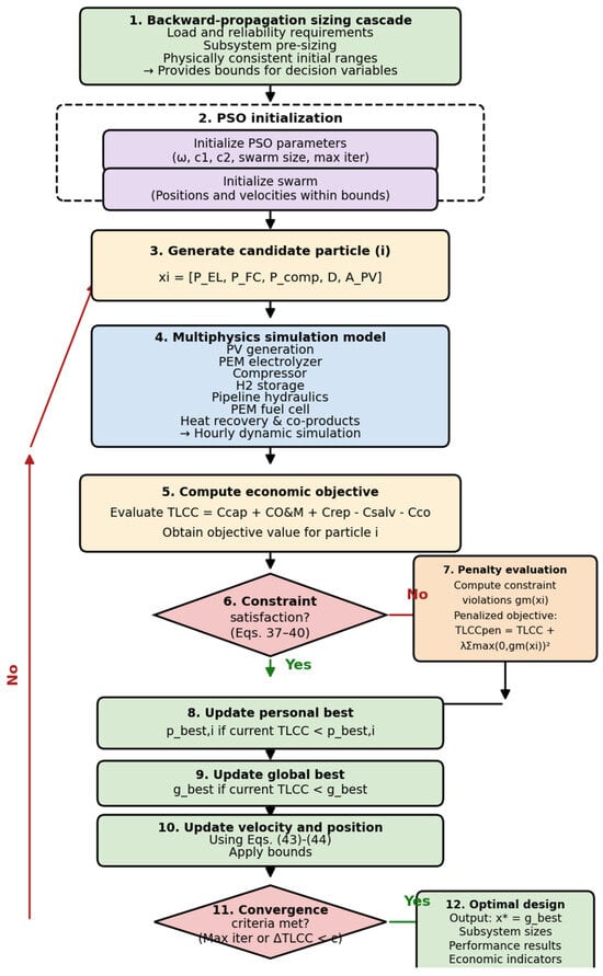
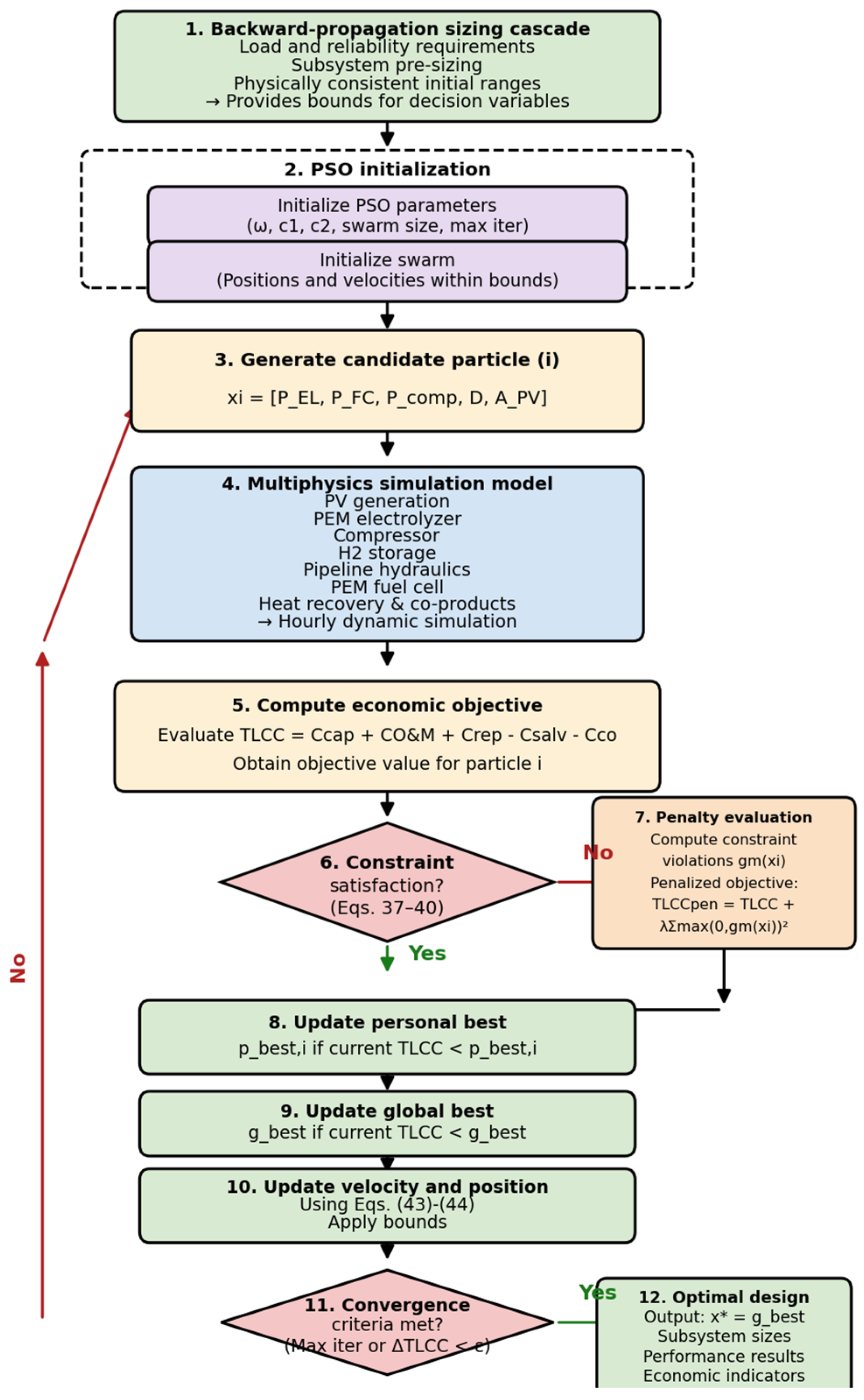
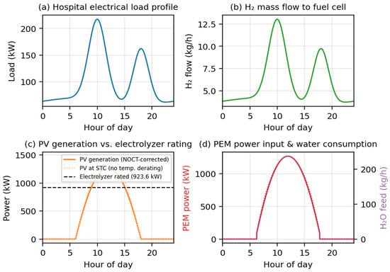
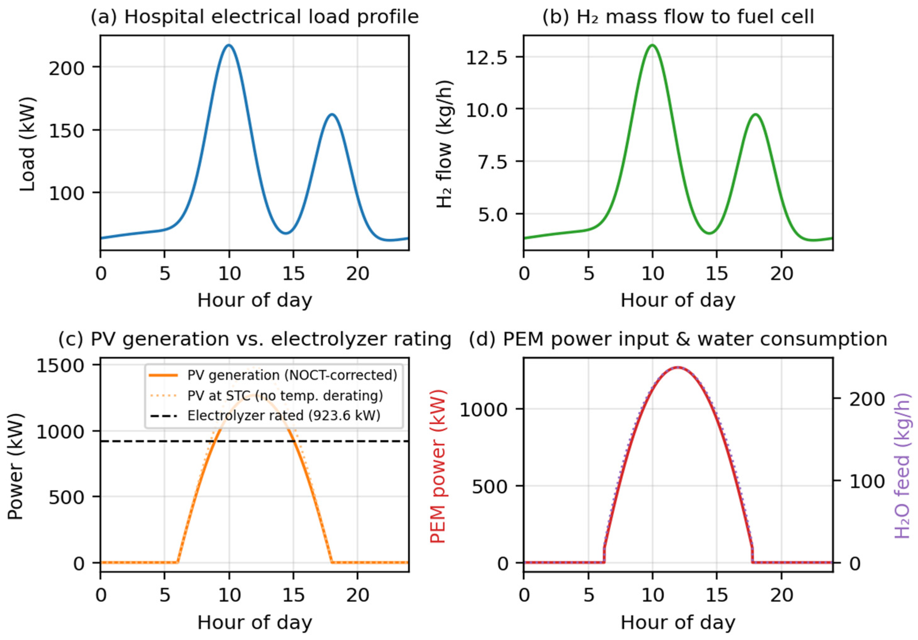
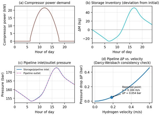
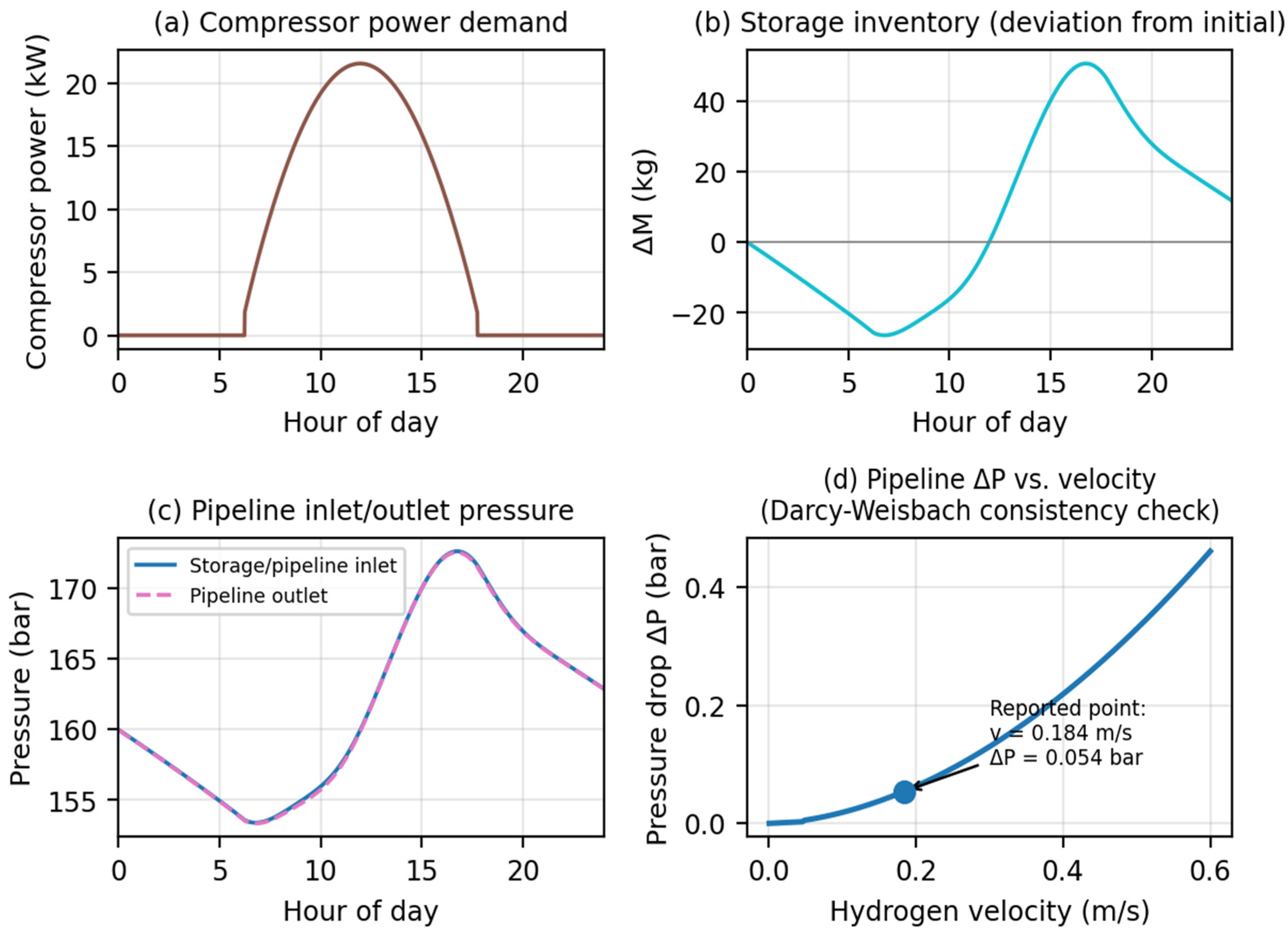
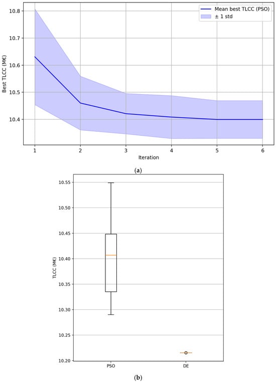
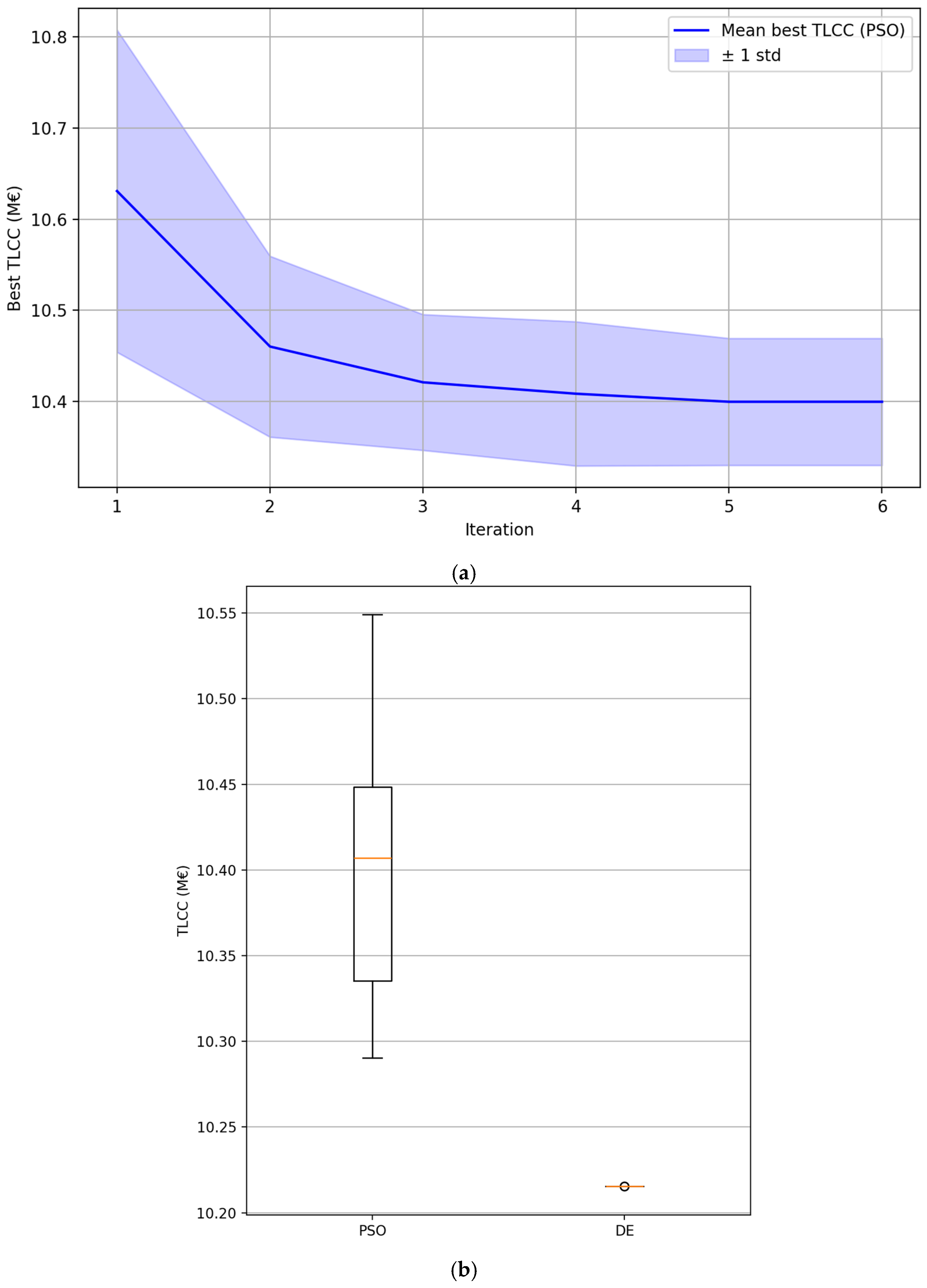
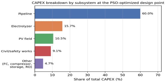
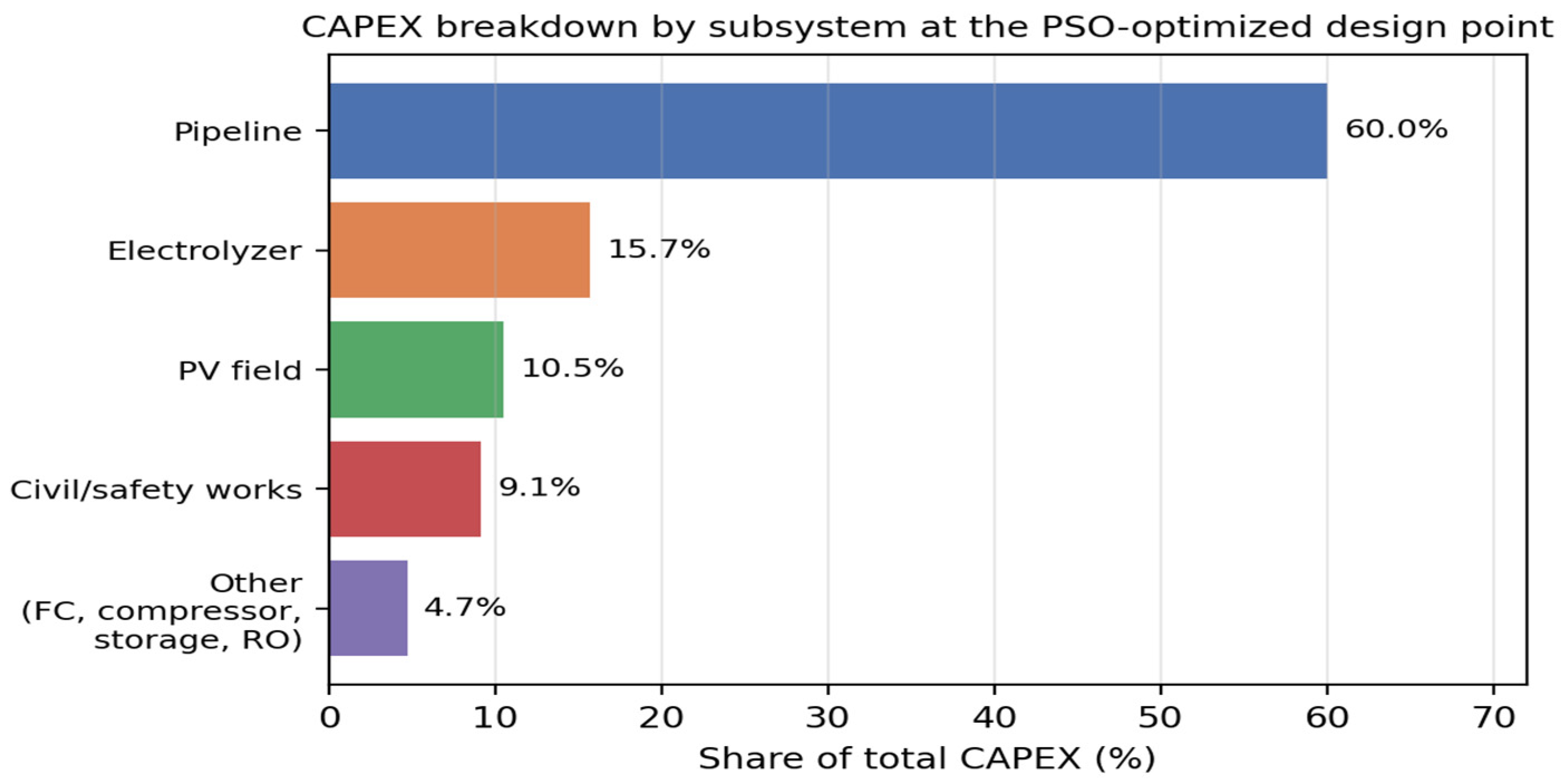
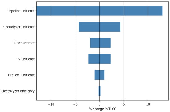
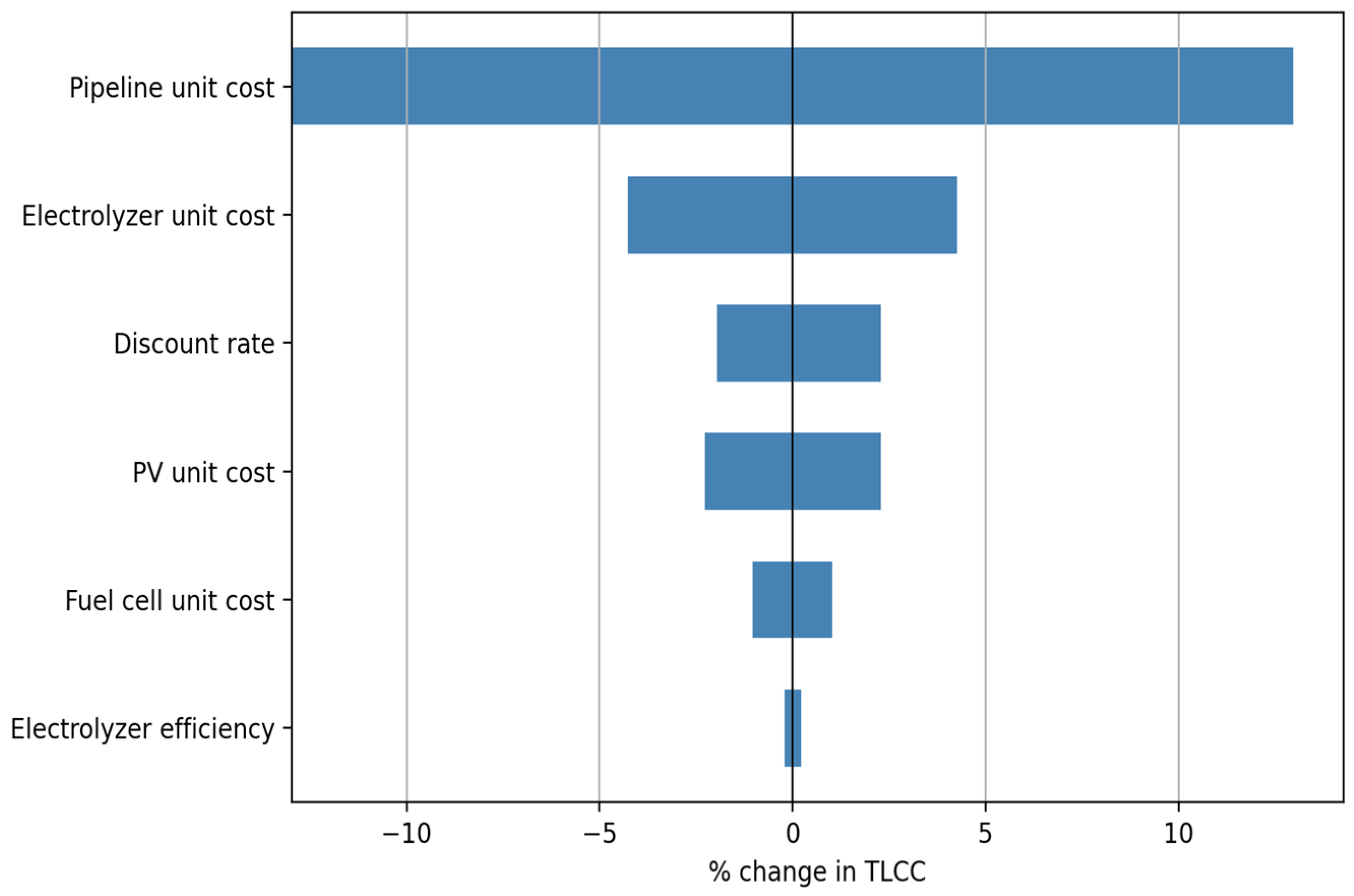

Disclaimer/Publisher’s Note: The statements, opinions and data contained in all publications are solely those of the individual author(s) and contributor(s) and not of MDPI and/or the editor(s). MDPI and/or the editor(s) disclaim responsibility for any injury to people or property resulting from any ideas, methods, instructions or products referred to in the content. |
© 2026 by the authors. Licensee MDPI, Basel, Switzerland. This article is an open access article distributed under the terms and conditions of the Creative Commons Attribution (CC BY) license.