


Abstract
Hydrogen blending into natural gas grids can support early renewable hydrogen deployment, but admissible injection depends on local gas flow, blending limits, and upstream hydrogen concentrations. This paper analyses these effects for a regional high-pressure gas-grid section in Styria, Austria, with two hydrogen injection points. A transient gas-network model derives time- and location-dependent injection limits, which are integrated into an electrolyser dispatch optimisation with fixed trailer demand and annual gas-grid injection demand. Three cases are compared: unrestricted injection, a “CH4-based” limit without upstream hydrogen, and an “H2-aware” case representing potential upstream hydrogen injection. For the analysed configuration, blending constraints shift operation away from favourable electricity-price periods, particularly when low prices coincide with reduced gas demand. In the 2025 reference case, the “H2-aware” constraint increases the electricity-cost contribution from 4.22 to 5.45 EUR/kgH2. A robustness analysis using electricity-price series for 2020, 2022, and 2025 shows that the “H2-aware” constraint increases the electricity-cost contribution by 15.8–29.1% relative to unrestricted injection. The results demonstrate that dynamic gas-grid constraints should be considered when assessing blending-based electrolyser projects, while the quantitative findings remain specific to the analysed network and assumptions.
1. Introduction
1.1. Motivation and Background
Hydrogen is expected to play an important role in the transition towards climate-neutral energy systems. The European Commission’s hydrogen strategy identifies renewable hydrogen as relevant for industrial applications, transport applications that are difficult to electrify, and renewable energy storage, including long-duration and seasonal balancing [1]. Key application areas therefore include parts of the chemical industry, iron and steel production, high-temperature industrial processes, long-distance transport, shipping, aviation, and energy-system flexibility.
Despite strong policy support, the development of the European hydrogen economy remains slower than long-term targets imply. Hydrogen Europe’s Clean Hydrogen Monitor 2025 reports 571 MWel of operational water electrolysis capacity in Europe by July 2025, which remains far below the EU target of 6 GWel by 2024 and 40 GW by 2030 [1,2]. For electrolytic hydrogen, electricity procurement is one of the dominant cost drivers. Therefore, electricity price exposure, capacity factor, and the operating schedule of electrolysers are decisive factors for hydrogen production costs [3,4].
A central barrier during the hydrogen market ramp-up is the coordination of production, demand, and infrastructure. Dedicated hydrogen infrastructure already exists in Europe, particularly in industrial and regional networks, and new hydrogen pipeline projects are being developed. However, a broadly available hydrogen transport network capable of connecting dispersed production sites with future demand centres is still emerging. Existing natural gas grids can therefore provide transitional short- to medium-term transport and storage functionality for renewable hydrogen while dedicated hydrogen infrastructure is planned and expanded [5,6,7,8].
As such, hydrogen blending into natural gas grids has been proposed as an interim option for integrating renewable hydrogen, supporting sector coupling, and enabling early electrolyser deployment before dedicated hydrogen infrastructure is widely available. Several pilot and demonstration projects have tested hydrogen admixture in existing gas infrastructure, including GRHYD in France and HyDeploy in the United Kingdom, which demonstrated blend shares up to around 20 vol.% under controlled conditions [7,8,9]. In Austria, recent hydrogen projects also illustrate the transitional relevance of existing gas infrastructure. Wien Energie operates a 3 MW proton exchange membrane (PEM) electrolyser with a gas-grid blending option; Energie Steiermark’s Renewable Gasfield in Gabersdorf combines photovoltaic generation, electrolysis, trailer filling, and gas-grid feed-in; and RAG Austria has demonstrated pipeline-based cross-border delivery of blended green hydrogen from Austria to Germany [10,11,12].
However, hydrogen blending is subject to technical and regulatory limits. Hydrogen changes the physical and combustion properties of the transported gas mixture, including energy density, Wobbe index, flow velocity, pressure losses, leakage behaviour, and material compatibility. These effects can constrain both transmission and distribution networks and may also depend on downstream end users, compressors, storage facilities, and connected gas appliances [6,7,8]. At the European level, studies indicate that hydrogen blending of approximately 5–10 vol.% is often considered feasible in the near term without major infrastructure modifications, while higher shares of 15–20 vol.% may require adaptations in infrastructure and end-use installations [6,13]. In Austria, the technical rule ÖVGW G B210:2021 06 allows up to 10 vol.% hydrogen in the natural gas grid [14].
For electrolyser projects that rely on grid injection, these blending limits directly influence how much hydrogen can be fed into the grid at a given location and hour. The admissible injection volume depends on the local gas flow, the existing hydrogen concentration in the gas stream, and the downstream gas-quality constraints. Consequently, static assumptions about annual feed-in capacity or fixed blending shares can misrepresent the actual operating potential of an electrolyser. This is especially relevant in networks with multiple hydrogen injection points, where upstream injection can already increase the hydrogen concentration in the gas stream and thereby reduce the remaining blending potential at downstream locations. Previous studies have shown that hydrogen concentrations in natural gas networks can vary over time and space, particularly when injection and demand profiles are time-dependent or when several injection points interact [15,16]. The need for dynamic gas-grid modelling has also been analysed in previous work by the authors, where the DynANA framework was developed for time-dependent hydrogen blending simulations with multiple injection points and compared with steady-state approaches [17,18]. These results show that steady-state approaches can misrepresent hydrogen concentrations because they do not capture temporal and spatial variations in gas flow and hydrogen transport. This can lead to an under- or overestimation of injection potentials and to a misjudgement of concentration limits. The present study therefore builds on these findings and focuses on how dynamically derived injection limits affect electrolyser dispatch and hydrogen production costs.
In parallel, a substantial body of research has developed methods for optimising electrolyser operation and assessing the levelised cost of hydrogen (LCOH). These studies typically minimise electricity procurement costs or total hydrogen production costs by adjusting electrolyser dispatch to renewable generation profiles, electricity market prices, storage availability, degradation effects, or hydrogen demand requirements. Approaches include linear and mixed-integer optimisation, dynamic programming, techno-economic dispatch models, and market-based operating strategies. For example, dynamic PEM electrolyser operation has been shown to reduce LCOH by exploiting time-varying electricity prices, while recent grid-connected studies develop bidding or dispatch strategies to reduce LCOH under wholesale electricity market conditions [19,20,21,22]. However, these studies generally represent hydrogen offtake through aggregate demand, storage, or market constraints and do not resolve the location- and time-dependent admissible feed-in capacity of the gas grid.
This leaves an important gap for electrolyser projects that rely on hydrogen blending. Treating the gas grid as an unrestricted sink can overestimate electrolyser utilisation and underestimate hydrogen production costs. Incorporating local gas flows, blending limits, and upstream hydrogen concentrations can instead shift electrolyser operation towards hours with sufficient injection potential and reveal location-specific effects on the resulting levelised cost of hydrogen.
1.2. Aim and Outline
This study investigates how local gas-grid constraints related to hydrogen blending affect the operation of an electrolyser and the resulting hydrogen production costs. The central hypothesis is that time- and location-dependent blending limits reduce the feasible grid feed-in of hydrogen, alter the cost-minimising operating schedule of the electrolyser, and increase hydrogen production costs compared with an unrestricted feed-in assumption. A second hypothesis is that, in a prospective multi-injection scenario, upstream hydrogen injection can reduce the remaining admissible injection potential at downstream locations and thereby intensify the operational and economic impact of blending constraints.
To test these hypotheses, a section of the Austrian gas grid is modelled using topological pipeline data and hourly gas demand profiles. Dynamic gas flow simulations are used to derive location- and time-dependent hydrogen injection limits. These limits are then integrated into an optimisation model for the dispatch of an electrolyser that supplies both, a daily on-site hydrogen demand and an annual hydrogen demand transported through the gas grid. The optimisation minimises hydrogen production costs while considering electricity prices, demand requirements, and blending constraints.
Three injection constraint cases are analysed: first, the “no-injection-limit” case, in which hydrogen feed-in to the gas grid is unrestricted by blending constraints; second, the “CH4-based” case, in which hydrogen injection is limited by the local methane flow and the maximum admissible hydrogen concentration; and third, the “H2-aware” case, which represents a prospective multi-injection scenario in which upstream hydrogen injection occupies part of the admissible blending margin at the downstream node.
The remainder of the paper is structured as follows. Section 2 describes the case study, the gas demand model, the dynamic gas-grid simulation in DynANA (Dynamic Analysis for Network Applications) [18], the electrolyser dispatch optimisation framework using IESopt (Integrated Energy System Optimization) [23], and the performance indicators used for evaluation. Section 3 presents the resulting gas demand distribution, upstream hydrogen propagation, injection limits, and downstream electrolyser operation under the three injection constraint cases. Section 4 discusses the interpretation of the cases, the implications for electrolyser operation and hydrogen production costs, and the main modelling limitations. Section 5 summarises the main findings and outlines directions for future work.
2. Materials and Methods
This section describes the modelling frameworks and data used to analyse the impact of hydrogen blending constraints on electrolyser operation and costs. It first introduces the case study and overall system setup (Section 2.1), followed by the calculation and spatial allocation of gas demand (Section 2.2). Based on this, the relevant part of the gas network is modelled in DynANA to determine time-dependent hydrogen injection constraints (Section 2.3). The operation of the electrolysis systems is then represented and optimised in IESopt (Section 2.4). Finally, the considered cases are evaluated using operational and economic performance metrics (Section 2.5).
2.1. Overview of the Case Study
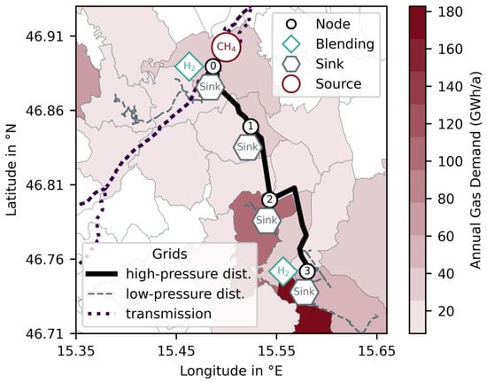
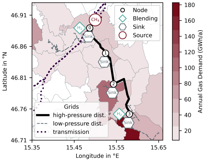
The study region is located in Styria, Austria, where hydrogen injection into the gas grid is planned [11]. This region is connected to the transmission pipeline TAG [24] via a regional high-pressure distribution pipeline. Additionally, local low-pressure distribution networks are connected to the regional grid. The existing project injects hydrogen approximately 20 km downstream from the transmission grid connection into the high-pressure distribution grid. In addition, a second injection location is assumed directly downstream of the connection between the transmission and the regional grid (see Figure 1).
Figure 1.
Studied gas-grid section in Styria, Austria, including the transmission grid, high-pressure distribution pipeline simulated in this work, connected low-pressure distribution grids, hydrogen blending points, and modelled sink and source nodes. Blending node 0 corresponds to the upstream electrolyser, located directly at the transmission-grid connection. Blending node 3 corresponds to the downstream electrolyser, located approximately 20 km further downstream.
Hydrogen injection is restricted by the current regulatory concentration limit of 10 vol.% in Austrian gas grids [14]. This limit, together with the gas flow at the injection node and the hydrogen concentration in the gas stream prior to injection, determines the available injection potential. Electrolysers are installed at both injection points and must meet local on-site demand as well as demand supplied via hydrogen blending through the gas grid. The objective of this study is to investigate the impact of grid restrictions on the operation of the electrolysis plants. Therefore, the analysis is restricted to the gas flow between the two injection points, and only this section of the network is simulated.
To analyse the interaction between both injection points, the relevant section of the gas grid is represented by a simplified nodal network. For this purpose, the modelled region is divided into grid cells, which are mapped to network nodes, and hourly gas demands are assigned based on publicly available district-level demand data and sector-specific load profiles (see Section 2.2).
The resulting network model is implemented in DynANA and used to simulate gas flows between the two electrolysers (see Section 2.3). The hydrogen injection profile of the upstream electrolyser is used as an input to the gas-grid simulation. The resulting time-dependent injection potential at the downstream injection point is then used as a constraint for the electrolyser optimisation.
The injection profiles are determined by optimising the dispatch of the electrolysis systems in IESopt, an optimisation framework for energy system modelling (see Section 2.4).
2.2. Gas Demand Model
2.2.1. Spatial Grid Construction and Node Allocation
To derive spatially resolved gas demands, the network topology and information on pressure levels and network hierarchy are used to construct a simplified nodal representation of the grid. The available pipeline data are first classified into the main network (simulated), connected local distribution grids, nearby pipelines that are not connected to the simulated network, and transmission lines. Nodes are defined along the simulated pipeline, including start and end points, as well as locations where local distribution grids connect.
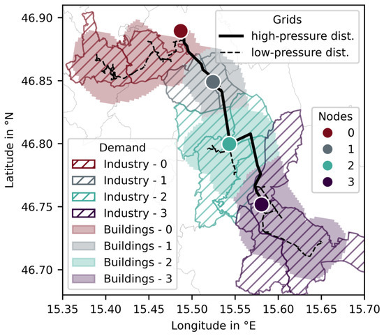
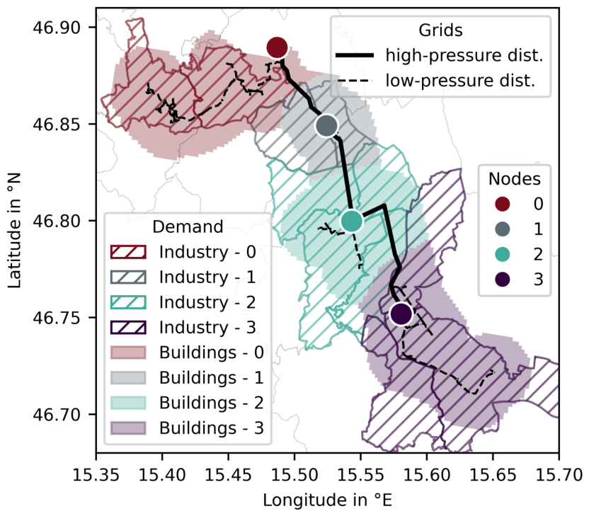
A buffer area of 2 km around the main network and connected local distribution pipelines is defined and subdivided into grid cells of 200 m×200 m. Each cell is assigned to the nearest pipeline segment of the main network, connected grids, or nearby pipelines that are not connected to the simulated network. The grid cells are subsequently mapped to simulated network nodes. Cells associated with the main network are assigned to the nearest node, while those belonging to connected grids are linked to the closest intersection node. Cells associated with nearby pipelines that are not connected to the main network are excluded. As a result, each remaining cell is uniquely assigned to a network node (see Figure 2).
Figure 2.
Spatial allocation of annual gas demand to network nodes in the studied region. Industrial demand is assigned directly to the corresponding nodes, while household and building demand is distributed across grid cells and aggregated at the nearest network node.
2.2.2. Sectoral Gas Demand Estimation and Temporal Disaggregation
Based on this spatial representation, gas demand is estimated at the district level and subsequently allocated to the network nodes. Annual energy demand data for sector industries (“Industrie und Gewerbe”), households (“Wohnen”), and buildings (“Dienstleistungen”) are obtained from the Energy-Mosaik dataset [25]. Using data from the Energy Transition Model (ETM) [26], the share of natural gas in total energy demand is estimated as 38.1% for industries, 48.9% for households, and 46.6% for buildings, which then yields annual gas demand for each district and sector (A scenario with default parameters for Austria was generated using the ETM. The results for “primary energy use” were used to determine the share of natural gas in total energy consumption for each sector). Sectoral demand is then allocated within each district. Household and building demands are spatially disaggregated by assuming a uniform distribution across the district and assigning the resulting demand to grid cells of one hectare. Only the demand located in cells within the defined buffer zone around the simulated gas-grid section or the connected local distribution grids is assigned to the corresponding modelled network nodes. Demand in cells outside this buffer zone, as well as demand associated with nearby but unconnected pipelines, is excluded from the simulated network.
For the industrial sector, demand is assigned at district level to the corresponding network node if the district is connected to the analysed gas-grid section. This approach assumes that industrial gas demand is spatially concentrated and supplied through the gas grid in connected districts. Since measured industrial connection points and nodal load data were not available, the full district-level industrial gas demand is assigned to the connected node as an approximation (see Figure 2).
To obtain time-resolved demand profiles, sector-specific hourly load profiles from the ETM are used. These profiles differ across sectors and are scaled to match the annual demand at each node. The resulting sectoral profiles are then aggregated into a single hourly load profile per network node, which serves as input to the gas-grid simulations.
2.3. DynANA Model
A dynamic gas-grid model is required for this study because the admissible hydrogen injection at the downstream node depends on the local methane flow and on the hydrogen concentration already present in the gas stream. Both quantities vary over time. A static blending constraint would either have to be defined conservatively to ensure compliance with the 10 vol.% limit at all times, or it could overestimate the admissible injection during periods with low methane flow or high upstream hydrogen concentration. Therefore, DynANA is used to derive time-dependent injection limits, which are then transferred to the electrolyser optimisation in IESopt. The full numerical formulation of DynANA is described in [17,18] and the following paragraphs summarise the elements required for the coupling with the electrolyser optimisation.
DynANA represents the pipeline with diameter D and cross-sectional area A as one-dimensional isothermal flow at fixed temperature T and solves the fluid-dynamic balance equations,
for the pressure p, the mass flow q, and the methane concentration c.
The gas mixture is described by the real-gas equation of state
where is the gas density, Z is the compressibility factor, and is the composition-dependent specific gas constant. The compressibility factor is calculated using the Papay correlation, with the pseudo-critical pressure and temperature determined using Kay’s mixing rule. The complete formulation is provided in [17,18].
The balance equations are solved using a finite-volume approach. The pipeline is discretised into control volumes, for which the mixture properties are updated in each time step. These properties include Z, the friction factor f, and . Hydrogen transport is represented by convective transport with the gas flow, while physical diffusion is neglected.
Boundary conditions are represented by sources and sinks. The upstream boundary is modelled as a pressure-controlled methane source. Hydrogen injection is represented as a flow-controlled source. Gas demand is represented by energy-controlled sinks. For each sink and time step, the lower heating value of the local methane–hydrogen mixture is calculated and the withdrawn mass flow is adjusted such that the specified energy demand is satisfied.
The admissible hydrogen injection at the downstream node is calculated from the methane concentration in the incoming gas stream and the energy demand at the corresponding sink. Since the blending limit is defined as a volume concentration, the limit of 10 vol.% hydrogen is converted into the corresponding minimum methane mass fraction . For each time step, the total gas mass flow that would satisfy the same energy demand with a methane–hydrogen mixture containing 10 vol.% hydrogen is calculated as
where is the energy demand, and is the lower heating value of the methane–hydrogen mixture at the 10 vol.% hydrogen limit.
The maximum hydrogen mass flow contained in such a gas stream is then given by
where is the methane mass fraction corresponding to the 10 vol.% hydrogen limit. The hydrogen mass flow already present in the incoming gas stream is calculated as
where is the current gas mass flow and is the current methane mass fraction. The remaining admissible hydrogen injection is then obtained as
This time-dependent injection limit is transferred to IESopt and used as an upper bound for hydrogen feed-in from the downstream electrolyser.
The model for this study is based on the topology and network levels of the real gas grid [27] (see Figure 1).
The upstream connection of the regional distribution pipeline to the transmission grid is represented by a pressure-controlled methane source with a constant pressure of 40 bar. This source defines the upstream boundary of the model and is represented by network node 0. The first hydrogen injection is implemented directly downstream of the source as a flow-controlled feed-in. The gas demand of the surrounding districts is represented by an energy-controlled sink at this node.
The modelled regional network connects the first injection point at node 0 with the second injection point at node 3. This section is divided into three pipeline segments connected via nodes 1 and 2. All segments are represented by pipes with a diameter of m and an absolute roughness of mm. Additionally, the gas temperature is assumed to be constant at K. The hydrogen injection at node 3 is also modelled as a flow-controlled feed-in.
Since gas is withdrawn at the intermediate nodes, the gas flow rate and velocity decrease in the downstream direction. At lower velocities, a finer spatial discretisation is required to maintain the numerical accuracy of the hydrogen concentration profile. To ensure sufficient spatial resolution throughout the network, the number of control volumes N is increased for downstream pipe segments (see Table 1). The spatially discretised system is solved using the adaptive FBDF algorithm for stiff differential-algebraic equation systems. The absolute and relative solver tolerances are both set to . Since FBDF uses adaptive time stepping, no fixed internal simulation time step is prescribed.
Table 1.
Pipeline segment parameters used in the DynANA gas network model. The table lists the node connections, segment lengths L, number of control volumes N, and resulting spatial resolution .
The intermediate nodes correspond to locations where local distribution networks are connected to the regional distribution pipeline. These local distribution grids are not modelled explicitly in DynANA. Instead, they are used to spatially aggregate gas demand as described in Section 2.2. The resulting nodal gas demands are implemented as energy-controlled sinks at the corresponding nodes. At each time step, the withdrawal rate is adjusted according to the methane–hydrogen composition such that the specified energy demand is satisfied exactly.
2.4. Electrolysis
Both electrolysis systems are modelled as PEM electrolysers. PEM electrolysers are suitable for the dynamic operating conditions considered in this study because they have short response times and a wide operating range, which allows them to adapt rapidly to fluctuating electricity prices and grid-related injection constraints [20,28]. Therefore, PEM technology is appropriate for analysing flexible electrolyser dispatch under time-dependent boundary conditions.
2.4.1. Optimisation Framework–IESopt
IESopt is a modular energy system modelling framework that can be used to optimise the operation of integrated multi-carrier systems based on a cost-minimisation formulation. It determines time-resolved operational decisions for system components, including energy conversion, storage, and grid interactions. In this study, IESopt is applied to compute the cost-optimal operational strategy of the electrolyser under dynamic boundary conditions and grid constraints.
The electrolysis system described in this work is represented as a coupled electricity–hydrogen system with electricity grid connection, hydrogen production, trailer-based hydrogen demand requiring additional compression, and hydrogen feed-in to an external gas grid. Electricity is purchased from the external electricity market and transferred to an internal electricity node. The electrolyser is represented by a binary on/off-status variable and a continuous load variable. When the electrolyser is switched off, its load is zero. When it is switched on, its load can vary continuously between the specified minimum load and the installed capacity. The model therefore allows partial-load operation while enforcing the minimum-load constraint. The produced hydrogen is routed to an internal hydrogen node and can either be injected into the external gas grid, constrained by a time-dependent feed-in limit from the gas-grid simulation (see Section 2.3), or compressed into trailers to satisfy additional hydrogen demand.
2.4.2. Model Inputs and Assumptions
The techno-economic input parameters of the electrolysis system are based on data from the Levelised Cost of Hydrogen Calculator of the Clean Hydrogen Observatory [29] for PEM electrolysis. These include a specific electricity consumption of 53.3 kWh/kgH2, a capital expenditure of 2593 kEUR/MWel, a technical lifetime of 25 years, a stack lifetime of 60,000 h, stack replacement costs of 15% of the initial investment, and fixed operation and maintenance (O&M) costs of 2% of CAPEX (The default value of the European Hydrogen Observatory reports 2503 EUR/kW in 2024 money terms. To express all cost inputs in 2025 money terms, this value was adjusted using the Austrian annual inflation rate of 3.6% for 2025). Stack replacement costs are internalised as variable operating costs by distributing them over the stack lifetime, resulting in a cost contribution proportional to electrolyser operation. Based on the lower heating value of hydrogen (33.33 kWh/kgH2), the electrolyser efficiency is approximately 0.625 MWhH2/MWhel.
The compressor parameters are based on default data from HyTool [30] and include a specific electricity consumption of 1.28 kWh/kgH2, a technical lifetime of 15 years, a CAPEX of 4.14 kEUR/(kgH2/h) and fixed O&M costs of 3% of CAPEX. The compressor capacity is 48 kWel, which was determined based on the maximum hydrogen output of the electrolyser.
The reference analysis uses Austrian day-ahead electricity prices for 2025 at a 15 min resolution [31]. To assess the robustness of the results with respect to the selected electricity-price year, the optimisation of the downstream electrolyser is repeated using day-ahead price time series for 2020 and 2022. To ensure identical annual time horizons and direct comparability between the price years, all observations for 29 February were removed from the 2020 time series, resulting in 365-day data sets for each analysed year.
Electricity grid charges are represented by a power-based component of 66,076 EUR/(MW a) and a consumption-based component of 37.7 EUR/MWh [32]. These charges are held constant across all electricity-price years and injection-constraint cases.
Hydrogen demand is represented by a time-dependent trailer supply profile and a fixed annual gas-grid injection requirement. Both demand inputs are held constant across all electricity-price years and injection-constraint cases.
The installed capacities of the electrolysers are exogenous case-study assumptions and were not derived from a plant-sizing optimisation. They were selected to represent small-to-medium PEM electrolysis systems and to create a feasible operating problem in which both on-site demand and gas-grid injection demand can be supplied. The objective of this study is therefore not to identify the cost-optimal electrolyser size, but to isolate the operational and economic impact of gas-grid injection constraints for a fixed system configuration.
2.4.3. Upstream Electrolysis
The upstream electrolyser is included to generate a realistic hydrogen injection profile. Its operation is not part of the core analysis; however, its parameters are included for completeness.
The electrolyser has an installed capacity of 3 MW and supplies an on-site hydrogen demand of 20 MWh per day—based on the lower heating value of hydrogen of 33.33 kWh/kg—that must be fully supplied daily between 06:00 and 22:00. In addition, an annual hydrogen demand of 6000 MWh is delivered via injection into the gas grid, in compliance with grid restrictions.
The admissible hydrogen injection is determined based on the local gas flow and the regulatory concentration limit of 10 vol.%. For each time step, the total downstream gas demand is aggregated, and the corresponding maximum hydrogen injection is calculated assuming this concentration limit.
2.4.4. Downstream Electrolysis
The second electrolyser, which is the focus of the analysis, has an installed capacity of 2 MW and supplies an on-site hydrogen demand of 10 MWh per day—based on the lower heating value of hydrogen of 33.33 kWh/kg—that is connected overnight, between 18:00 and 10:00. In addition, an annual hydrogen demand of 4000 MWh is delivered via injection into the gas grid and analysed for three distinct cases. Trailer supply and gas-grid injection are modelled as mandatory hydrogen sinks without an explicit priority order. The optimisation may therefore allocate hydrogen to either sink whenever the respective demand constraint can be satisfied, while the daily trailer demand and the annual gas-grid injection demand must be fulfilled. In the “no-injection-limit” case, no restrictions on hydrogen injection are assumed. In the “CH4-based” case, hydrogen injection is limited by the methane flow at the injection node and the maximum admissible hydrogen concentration of 10 vol.%. In the “H2-aware” case, hydrogen from the upstream electrolyser is already present in the gas stream, such that the injection potential depends on both the local gas flow and the existing hydrogen concentration.
2.5. Performance Metrics and Evaluation
The electrolysis system is optimised over a full-year time horizon with a resolution of 15 min. The resulting solution represents the cost-minimal operation that satisfies the defined hydrogen demand under the given technical and grid-related constraints. To compare the different cases, both operational and economic performance metrics are evaluated.
From an operational perspective, the analysis focuses on time-resolved hydrogen injection into the gas grid, including the injection profile for a representative day and aggregated hydrogen injection over quarterly periods. In addition, electrolyser operation is assessed based on its load profile and the number of hours during which the injection limit restricts electrolysis operation. This value is defined as
where denotes the set of all time steps in the simulation horizon, is the temporal resolution, is the injected hydrogen, is the total hydrogen production, is the maximum possible hydrogen production, and denotes the number of elements in the set.
To evaluate economic performance, the levelised cost of hydrogen (LCOH) is defined as the ratio of total annualised system costs to total hydrogen production over the simulated year. Cost components include annualised capital expenditures, fixed and variable operating costs, electricity procurement costs, and grid-related charges. Capital expenditures are annualised using an interest rate of 6%. Cost data from different source years are converted to 2025 money terms where necessary, and all results are presented in 2025 money terms. Particular attention is given to electricity cost contributions to assess the impact of grid constraints and injection limitations on electrolyser operation and hydrogen production costs.
The electricity-price years are characterised using the daily electricity-price spread, defined as the difference between the maximum and minimum day-ahead price within each calendar day. For each price year, the electricity-cost contributions of the constrained cases are compared with the corresponding “no-injection-limit” case. The relative increase is determined as the percentage difference between the electricity-cost contribution of the constrained case and that of the “no-injection-limit” case for the same price year.
3. Results
The results show how upstream hydrogen blending constraints and prospective upstream hydrogen injection affect the injection potential and operation of a downstream electrolyser. First, the gas demand, upstream electrolysis, and resulting hydrogen concentration in the gas grid are described. The downstream electrolysis is then evaluated with respect to daily operation, seasonal injection patterns, load duration, and electricity-related hydrogen production costs.
3.1. Gas Demand, Upstream Electrolysis and Grid Simulation
The gas demand ranges from 45 GWh to 237 GWh per year across the defined nodes, with the largest demands occurring at the end of the network, i.e., at nodes 2 and 3. The high demand at the final node ensures a sufficiently large gas flow for the second hydrogen injection point. In total, 494 GWh of annual gas demand is connected to the modelled network section. Of this demand, 60% occurs during quarters Q1 and Q4, while the remaining 40% is distributed over quarters Q2 and Q3. During quarters Q2 and Q3, when space heating demand in buildings and households is lower, the gas flow is mainly maintained by industrial demand. This is particularly relevant at node 3, where more than 80% of the demand is attributed to the industrial sector (see Table 2).
Table 2.
Annual gas demand and share of industrial demand at each network node.
The operation of the upstream electrolysis is not part of the core analysis and therefore only briefly summarised to characterise the boundary conditions for the downstream system. To reduce hydrogen production costs, the electrolyser is preferably operated during hours with low electricity prices. However, its operation is constrained by the plant size, the time-dependent hydrogen demand, and the injection capacity of the gas grid.
These constraints are particularly relevant because gas-grid limitations and low electricity prices only partly occur during the same period. As described above, gas demand is lower during quarters Q2 and Q3, which reduces the available injection capacity. At the same time, low electricity prices in 2025 also occur mainly during these quarters due to high renewable electricity generation. The mean day-ahead electricity price is approximately 99 EUR/MWh, and more than 70% of the hours with below-average electricity prices occur in quarters Q2 and Q3. This temporal mismatch affects the electrolyser schedule and results in h, during which injection is restricted by the gas grid. This corresponds to 20% of the total injection hours.
This temporal mismatch not only affects the operating schedule of the upstream electrolyser, but also determines the hydrogen concentration entering the downstream part of the network. To illustrate this effect, the concentration profiles at the injection node and at the end of the modelled network are compared.
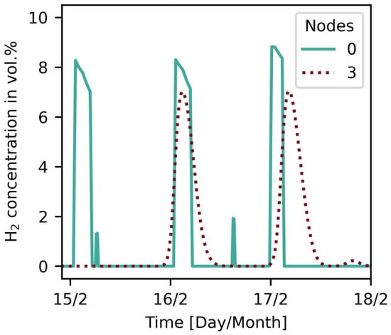
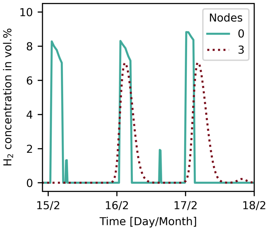
During winter, hydrogen injection is generally lower and occurs in comparatively short peaks. This allows the propagation of individual hydrogen packages through the network to be observed. The concentration increase reaches the downstream end of the modelled network with a delay of approximately 24 h. During transport, the concentration profile becomes broader, while the peak concentration is slightly reduced compared with the injection node. This behaviour reflects the numerical dispersion of the hydrogen package along the pipeline, as discussed in [18]. The results therefore show that very short and narrow hydrogen concentration peaks cannot be fully resolved by the gas-grid simulation, which should be considered when interpreting short-term concentration variations at downstream nodes (see Figure 3).
Figure 3.
The hydrogen concentration at the beginning (node 0) and the end (node 3) of the network for three days in February.
3.2. Downstream Electrolysis
The downstream electrolysis is analysed to assess how gas-grid injection limits affect operation, seasonal hydrogen injection, load duration, and electricity-related production costs. The comparison considers the “H2-aware” case, the “CH4-based” case, and the “no-injection-limit” case. This allows the local effect of methane-flow-based blending limits to be distinguished from the additional effect of prospective upstream hydrogen injection on downstream electrolyser operation.
3.2.1. Operational Impact of Hydrogen Injection Limits
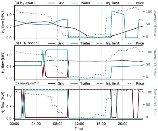
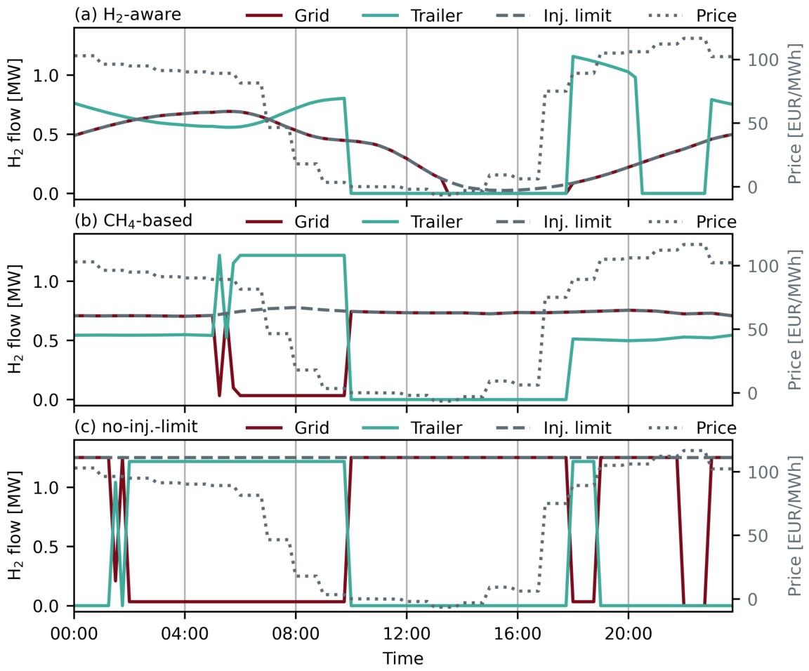
The downstream electrolysis shows distinct operating patterns for the three optimisation cases on a typical summer day. In the “H2-aware” case, grid injection is governed by the time-dependent injection limit. From midnight to approximately 10:00, the electrolyser operates close to its maximum hydrogen output of 1.25 MWH2, because both grid injection and trailer supply are available. After 10:00, the trailer demand window closes, and the admissible grid injection decreases to almost zero by 15:00. As a result, hydrogen production is strongly curtailed during the midday period, although electricity prices are lowest at this time. Operation increases again after 18:00, when trailer supply becomes available and the injection limit gradually rises (see Figure 4a).
Figure 4.
Operation of the downstream electrolyser on 4 July under the three injection constraint cases: (a) “H2-aware”, (b) “CH4-based”, and (c) “no-injection-limit”. The left axis shows hydrogen flows for gas-grid injection, trailer supply, and the admissible injection limit. The right axis shows the day-ahead electricity price.
In the “CH4-based” case, the admissible injection remains nearly constant at approximately 0.7–0.8 MWH2 over most of the day. Hydrogen can therefore still be injected into the gas grid during the low-price period. However, the injection limit remains below the maximum hydrogen output of the electrolyser. Between approximately 06:00 and 10:00, most of the production is used to satisfy trailer demand, and grid injection is reduced to the remaining available capacity. After the trailer demand window closes, grid injection increases to the “CH4-based” limit, but the electrolyser still cannot operate at full load when only grid injection is available. The “CH4-based” constraint is therefore less restrictive than the “H2-aware” case, but it still limits the use of low-price electricity (see Figure 4b).
In the “no-injection-limit” case, the operation is only determined by the electricity price signal and the trailer demand window. During periods with trailer demand, hydrogen production is directed to trailer supply and grid injection is reduced where necessary to remain within the maximum plant output. Since no priority is assigned between both hydrogen sinks, the allocation between trailer supply and grid injection can change as long as the demand constraints are fulfilled. Therefore, the operational interpretation of this period should focus on total electrolyser production rather than on the individual split between the two hydrogen sinks. After trailer demand is fully supplied in the morning, grid injection increases to the maximum hydrogen output and remains high throughout the low-price period (see Figure 4c).
3.2.2. Effect of Injection Constraints on Seasonal Operation
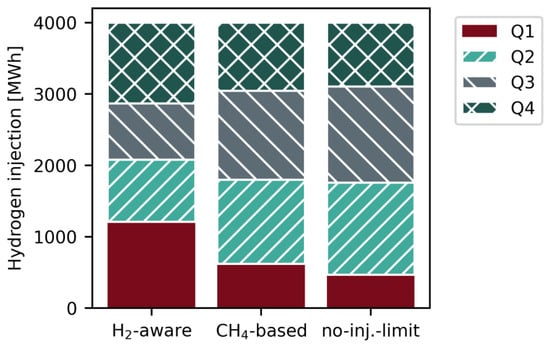
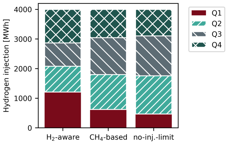
In the “H2-aware” case, injection during quarters Q1 and Q4 together accounts for approximately 59% of the annual injection. As discussed in Section 3.1, more than 70% of the hours with below-average day-ahead electricity prices occur during quarters Q2 and Q3. Therefore, the seasonal injection pattern is opposite to the electricity price signal. Under the “CH4-based” case, the seasonal distribution shifts towards quarters Q2 and Q3, which account for approximately 61% of the annual injection, compared with about 41% in the “H2-aware” case. Without an injection limit, this shift becomes even more pronounced, with approximately 66% of the annual injection occurring during quarters Q2 and Q3 (see Figure 5).
Figure 5.
Quarterly distribution of hydrogen injection into the gas grid for the downstream electrolysis under the three injection constraint cases.
3.2.3. Effect of Injection Constraints on Load Duration
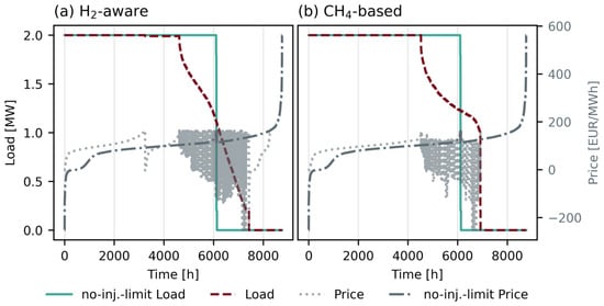
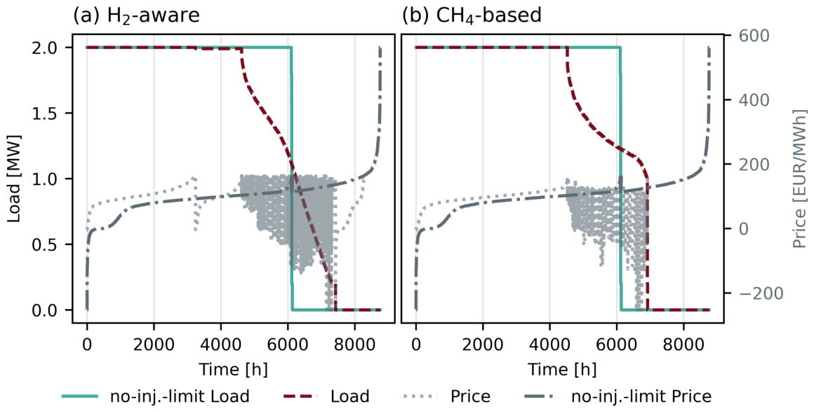
Without an injection limit, the electrolyser operates predominantly at full load and only drops to zero after approximately 6100 h. These full-load hours include the lowest electricity prices. In contrast, the “H2-aware” case reaches full load for only about 3200 h, decreases slightly to a load of 1.98 MW for another 1100 h and then shows a broad range of partial-load operation. Several low-price hours are therefore associated with reduced load or no load (see Figure 6a).
Figure 6.
Sorted load profiles of the downstream electrolyser and corresponding day-ahead electricity prices. Panel (a) compares the “H2-aware” case with the “no-injection-limit” case, while panel (b) compares the “CH4-based” case with the “no-injection-limit” case. For the sorting, the electrolyser load was first rounded to two decimal places. Time steps with the same rounded load were then sorted by increasing electricity price. The grey region between approximately 5000 and 7000 h represents the plotted electricity-price values in the partial-load region. In this interval, the electrolyser load is mainly determined by gas-grid injection constraints rather than by the electricity price. Therefore, the rounded load values occur in this region at strongly varying electricity prices, ranging from approximately −230 to 170 EUR/MWh.
The “CH4-based” case shows a less restrictive behaviour. Compared with the case without an injection limit, full-load operation is still reduced, but the reduction is smaller than in the “H2-aware” case. The electrolyser reaches full load for about 4500 h, followed by a partial-load range before operation drops to zero. The corresponding price curve shows that some low-price hours are still shifted to reduced-load operation, but this effect is less pronounced than for the “H2-aware” limit (see Figure 6b).
3.2.4. Electricity Cost Contribution and Robustness to the Electricity-Price Year
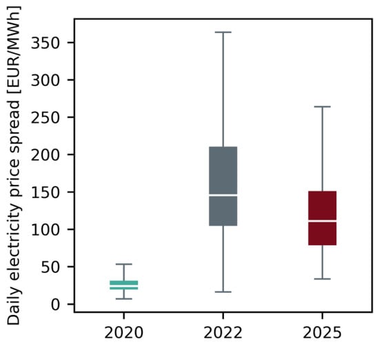
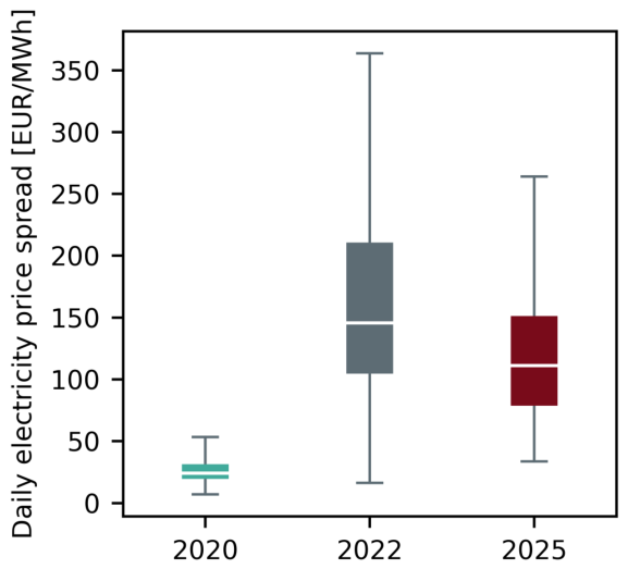
The analysed electricity-price years represent substantially different market conditions. Figure 7 compares the distribution of the daily electricity-price spread, calculated as the difference between the highest and lowest day-ahead price within each day. The year 2020 shows comparatively low and narrowly distributed daily spreads, whereas 2022 is characterised by substantially higher and more variable spreads. The 2025 price series lies between these two cases. The three years therefore provide distinct electricity-price environments for assessing the robustness of the cost effect caused by the gas-grid injection constraints.
Figure 7.
Distribution of the daily electricity-price spread for the analysed price years 2020, 2022, and 2025. The daily spread is defined as the difference between the maximum and minimum day-ahead electricity price within each day. Boxes indicate the interquartile range, horizontal lines the median, and whiskers the remaining distribution.
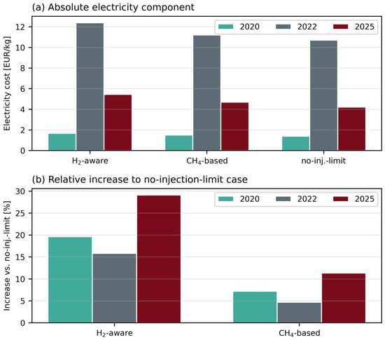
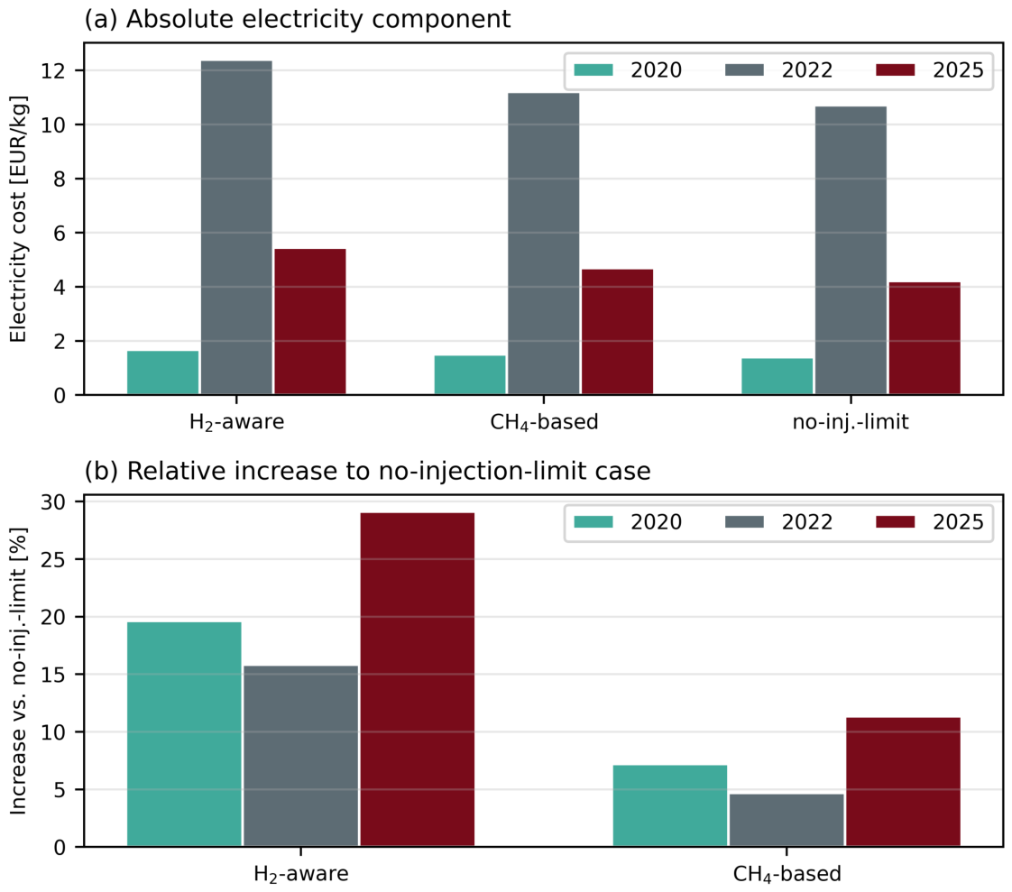
The “no-injection-limit” case results in the lowest electricity-cost contribution in all three price years, while the “H2-aware” case consistently results in the highest costs. For the 2020 price series, the electricity-cost contribution increases from 1.40 EUR/kgH2 in the “no-injection-limit” case to 1.50 EUR/kgH2 in the “CH4-based” case and 1.67 EUR/kgH2 in the “H2-aware” case. The corresponding values are 10.71, 11.21, and 12.40 EUR/kgH2 for 2022, and 4.22, 4.70, and 5.45 EUR/kgH2 for 2025 (see Figure 8a).
Figure 8.
Electricity-cost component of the levelised cost of hydrogen for the analysed electricity-price years and injection-constraint cases. Panel (a) shows the absolute electricity-cost contribution in EUR/kgH2. Panel (b) shows the relative increase in the electricity-cost contribution of the “H2-aware” and “CH4-based” cases compared with the “no-injection-limit” case of the corresponding price year.
Because the absolute price levels differ substantially between years, the constrained cases are additionally evaluated relative to the “no-injection-limit” case of the corresponding year. The “CH4-based” constraint increases the electricity-cost contribution by 7.1% in 2020, 4.7% in 2022, and 11.4% in 2025. The “H2-aware” constraint results in increases of 19.3%, 15.8%, and 29.1%, respectively. The direction of the cost effect is therefore consistent across all analysed price years, although its magnitude depends on the temporal structure of the electricity-price series (see Figure 8b).
The total LCOH follows the same ordering because the remaining cost components change only marginally between the cases. It ranges from 6.67 to 6.93 EUR/kgH2 for the 2020 price series, from 15.98 to 17.67 EUR/kgH2 for 2022, and from 9.48 to 10.70 EUR/kgH2 for 2025.
4. Discussion
The results demonstrate that the representation of gas-grid availability has a substantial influence on downstream electrolyser operation and electricity procurement costs. The comparison of the “no-injection-limit”, “CH4-based”, and “H2-aware” cases distinguishes between unrestricted injection, constraints imposed by the local methane flow, and the additional effect of hydrogen already present in the incoming gas stream. Across the analysed electricity-price years, the “H2-aware” constraint increases the electricity-cost contribution by 15.8–29.1% relative to the corresponding “no-injection-limit” case, while the “CH4-based” constraint results in an increase of 4.7–11.4%. These findings show that the economic impact of blending constraints is driven by the temporal alignment of electricity prices, local gas demand, and available injection capacity. The following discussion interprets these operational and economic effects and assesses the limitations arising from the representation of gas demand, grid operation, dynamic gas transport, and electrolyser design.
4.1. Interpretation of the Downstream Electrolyser Results
The comparison between the three cases shows that the representation of gas-grid availability directly affects the operating schedule of the downstream electrolyser. In the “no-injection-limit” case, the gas grid acts as an unrestricted sink, allowing hydrogen production to be concentrated in the economically most favourable electricity-price periods. This leads to the highest operational flexibility and the lowest electricity-cost contribution.
The “CH4-based” case restricts injection according to the local methane flow and the maximum admissible hydrogen concentration. Even without upstream hydrogen injection, these local blending constraints reduce the number of favourable operating hours and shift part of the hydrogen production towards periods with higher electricity prices. The “H2-aware” case introduces an additional restriction because hydrogen already present in the incoming gas stream occupies part of the available blending margin. This further reduces full-load operation and limits access to low-price electricity periods.
The economic effect is consistent across all analysed electricity-price years. Compared with the corresponding “no-injection-limit” case, the “CH4-based” constraint increases the electricity-cost contribution by 4.7–11.4%, while the “H2-aware” constraint results in an increase of 15.8–29.1%. The higher cost increase in the “H2-aware” case quantifies the additional effect that upstream hydrogen injection can have on a downstream injection point.
These findings indicate that electrolyser dispatch models representing the gas grid as an unrestricted sink may overestimate operational flexibility and underestimate electricity procurement costs. They also demonstrate that interactions between multiple hydrogen injection points become relevant when the available blending margin is shared within the same gas-grid section.
4.2. Limitations of Gas Demand and Grid Operation Modelling
A limitation of this study is the simplified representation of gas demand, as measured nodal loads and local demand profiles were not available for the analysed network section. Spatially and temporally resolved demand was therefore derived from district-level energy data and sector-specific standard load profiles. Household and building demand was disaggregated to hectare cells, with only the share close to the analysed gas-grid infrastructure assigned to the modelled network, while industrial demand was assigned at district level to the corresponding connected node. This approach distinguishes between spatially distributed building demand and concentrated industrial demand, but introduces uncertainty in the absolute nodal load distribution and its temporal variation. These uncertainties may affect local methane flows and the resulting hydrogen injection limits. A site-specific assessment would require measured nodal demand and load-profile data from the grid operator.
The temporal uncertainty is particularly relevant because gas demand profiles differ strongly between consumer groups. Household and building demand depends on weather conditions, building quality, and heating behaviour. Industrial demand depends on the sector, production process, and operating schedule. Some industrial consumers may operate with an almost constant load, while others may follow daily or weekly production patterns. These differences cannot be fully captured by standard sectoral profiles.
Additional uncertainty arises from the estimation of annual gas demand. In this study, the share of natural gas in total energy demand was derived from national-level data for Austria and applied to the study region. This approach does not fully represent local conditions, especially for industrial consumers, where the natural gas share depends strongly on the type of industry and process heat requirements. As a result, the absolute gas demand in the modelled section may differ from the actual demand in the local gas grid.
The gas-grid simulation is affected by assumptions on network operation and model boundaries. The model focuses on the high-pressure pipeline section between the two hydrogen injection points. Downstream infrastructure elements, such as low-pressure distribution grids, pressure-regulating stations, compressors, valves, and branches, are not explicitly modelled because they are outside the investigated pipeline section and do not directly affect the upstream-to-downstream hydrogen propagation analysed here. Their aggregated gas demand is represented through energy-controlled sinks at the corresponding nodes.
In particular, the upstream pressure was assumed to be constant at 40 bar. In reality, pressure levels can vary depending on seasonal demand, compressor operation, grid operation, and the use of linepack (Linepack refers to the quantity of gas stored within a pipeline due to its internal pressure and the compressibility of the gas. Variations in linepack provide operational flexibility by temporarily balancing differences between gas inflow and withdrawal). For a given energy demand at the sinks, a different pressure level would mainly affect gas density and flow velocity. It would therefore change the timing and duration of the hydrogen concentration profile arriving at the downstream injection node. Linepack operation could also influence admissible injection rates by changing pressure levels and available short-term buffering capacity. In particular, higher linepack in summer could increase admissible injection volumes to some extent.
These assumptions are especially relevant for the “H2-aware” case, because the remaining blending margin depends on the hydrogen concentration already present in the gas stream. A different pressure profile or linepack operation could shift hydrogen concentration peaks in time and thereby change their short-term coincidence with local gas demand and electricity prices. However, such timing shifts are not expected to remove the seasonal mismatch between low electricity prices and reduced gas demand in quarters Q2 and Q3. The main economic effect is therefore expected to be driven by the seasonal structure of gas demand and electricity prices, while the simplified pressure and linepack representation mainly affects short-term concentration timing and admissible injection volumes. Since measured pressure, flow, demand, and linepack operation data were not available, this uncertainty cannot be resolved in the present study.
However, the objective of this study is not to reproduce the exact gas demand and operating conditions at a specific site. Instead, the analysis aims to show how time-dependent gas flows and existing hydrogen concentrations affect electrolyser operation, injection schedules, and hydrogen production costs. The results should therefore be interpreted as representative for the analysed network configuration and assumptions.
4.3. Limitations of the Dynamic Gas-Grid Simulation
A further limitation is the numerical diffusion in the gas-grid simulation, as discussed in [18]. This effect is also observed in other dynamic gas network models [33,34] and reduces the accuracy of short-term hydrogen concentration profiles. In particular, numerical diffusion lowers the height of narrow concentration peaks and thereby increases their duration during transport through the pipeline. As a result, short and sharp hydrogen concentration changes at the downstream node may be smoothed in the simulation.
The spatial discretisation was chosen as a compromise between numerical accuracy and computational effort. A finer discretisation would reduce numerical diffusion, but would also increase simulation time. This uncertainty should therefore be considered when interpreting short-term concentration peaks. However, the broader temporal trends and the resulting impact on downstream injection potential remain suitable for the system-level analysis.
4.4. Implications for Electrolysis Design and Future Work
The downstream electrolysis results are specific to the analysed system configuration. The electrolyser capacity, on-site trailer demand, and annual hydrogen injection demand are fixed. The results therefore quantify the impact of gas-grid injection constraints on the operating schedule and electricity cost of this configuration, but they do not represent a cost-optimal plant design. A different annual injection demand could change both the utilisation of the electrolyser and the number of hours in which grid injection becomes restrictive. A sensitivity analysis on the annual hydrogen injection demand would therefore help to quantify how the injected hydrogen volume affects constrained operation, electricity cost, and total hydrogen production costs.
Plant sizing and additional flexibility options could change the economic outcome. A different electrolyser capacity could reduce constrained operation or improve the use of low-price electricity. Hydrogen storage could also decouple production from instantaneous gas-grid injection potential. However, storage would increase investment costs and would not remove the seasonal mismatch between low electricity prices and reduced gas flow in quarters Q2 and Q3. Its benefit would therefore depend on the trade-off between additional flexibility and additional capital cost. The electrolyser representation remains idealised, as start-up and shut-down losses, ramping limits, part-load efficiency variations, and degradation are not explicitly considered. The present study focuses on the system-level effect of gas-grid constraints rather than the detailed engineering of individual plants. These technical effects, particularly cycling-induced degradation, should be included in future work.
5. Conclusions
This study analysed how time- and location-dependent hydrogen blending constraints affect the operation and electricity-related production costs of an electrolyser connected to a natural gas grid. Dynamic gas-grid simulations were used to derive hydrogen injection limits, which were integrated into an electrolyser dispatch optimisation. Three representations of gas-grid availability were compared: unrestricted injection in the “no-injection-limit” case, a “CH4-based” limit determined by the local methane flow, and an “H2-aware” limit that additionally accounts for hydrogen already present in the incoming gas stream.
The results show that gas-grid constraints can substantially alter the cost-minimising dispatch of the downstream electrolyser. In the 2025 reference case, the “H2-aware” constraint shifts hydrogen production away from favourable electricity-price periods in quarters Q2 and Q3 and reduces full-load operation from approximately 6100 h to 3200 h. The electricity-cost contribution increases from 4.22 to 5.45 EUR/kgH2, corresponding to an increase of 29.1%, while the total LCOH increases from 9.48 to 10.70 EUR/kgH2.
The electricity-price-year analysis confirms that the direction of this effect is robust under substantially different market conditions. Relative to the corresponding “no-injection-limit” case, the “CH4-based” constraint increases the electricity-cost contribution by 4.7–11.4%, while the “H2-aware” constraint results in an increase of 15.8–29.1%. The magnitude of the effect depends on the temporal alignment of electricity prices, local gas demand, trailer demand, and available gas-grid injection capacity. Models that represent the gas grid as an unrestricted hydrogen sink may therefore overestimate operational flexibility and underestimate electricity procurement costs, particularly where several injection points share the available blending margin.
The quantitative results are specific to the analysed regional gas-grid section in Styria, the simplified network representation, electrolyser size, trailer demand, and fixed annual hydrogen injection demand. Future work should extend the analysis using measured gas demand, flow, and pressure data from grid operators. In addition, sensitivity analyses on electrolyser size, annual injection demand, hydrogen storage, and degradation effects would allow a more detailed assessment of cost-optimal system design under dynamic gas-grid constraints.
Author Contributions
Conceptualization, D.O., S.S. and S.R.; methodology, D.O., S.S. and S.R.; software, D.O. and S.S.; validation, D.O. and S.R.; formal analysis, D.O.; investigation, D.O.; resources, D.O. and S.S.; data curation, D.O. and S.S.; writing—original draft preparation, D.O. and S.R.; writing—review and editing, D.O., V.I., S.S. and S.R.; visualization, D.O.; supervision, V.I. and S.R.; project administration, S.R.; funding acquisition, S.R. All authors have read and agreed to the published version of the manuscript.
Funding
The conducted work is part of the “H2REAL” project which is supported with the funds from the Climate and Energy Fund and implemented in the framework of the RTI-initiative “Flagship region Energy”.
Data Availability Statement
Data on simulation inputs and results for dynamic gas-grid simulations with DynANA as well as results of the dispatch optimisation with IESopt are available under https://doi.org/10.5281/zenodo.21470282. All additional data are available upon request from the first author.
Acknowledgments
During the preparation of this manuscript/study, the authors used ChatGPT 5.5 for the purpose of formulation. The authors have reviewed and edited the output and take full responsibility for the content of this publication.
Conflicts of Interest
Author Dana Orsolits, Viktoria Illyés, Stefan Strömer and Stefan Reuter were employed by the company AIT Austrian Institute of Technology GmbH. The remaining authors declare that the research was conducted in the absence of any commercial or financial relationships that could be construed as a potential conflict of interest.
Abbreviations
The following abbreviations are used in this manuscript:
| CAPEX | Capital Expenditure |
| CH4 | Methane |
| DynANA | Dynamic Analysis for Network Applications |
| ETM | Energy Transition Model |
| EU | European Union |
| H2 | Hydrogen |
| IESopt | Integrated Energy System Optimization |
| LCOH | Levelised Cost of Hydrogen |
| O&M | Operation and Maintenance |
| PEM | Proton Exchange Membrane |
| TAG | Trans Austria Gasleitung |
| ÖVGW | Austrian Association for Gas and Water |
References
- European Commission. Hydrogen Strategy for a Climate-Neutral Europe. Communication from the Commission, COM(2020) 301 Final. 2020. Available online: https://eur-lex.europa.eu/legal-content/EN/ALL/?uri=COM:2020:301:FIN (accessed on 6 May 2026).
- Hydrogen Europe. Clean Hydrogen Monitor. 2025. Available online: https://hydrogeneurope.eu/reports/ (accessed on 6 May 2026).
- International Renewable Energy Agency. Green Hydrogen Cost Reduction: Scaling Up Electrolysers to Meet the 1.5 °C Climate Goal; Technical Report; International Renewable Energy Agency: Abu Dhabi, United Arab Emirates, 2020. [Google Scholar]
- European Hydrogen Observatory. Levelised Cost of Hydrogen (LCOH) Calculator Manual. In Proceedings of the Technical Report, Clean Hydrogen Joint Undertaking. Available online: https://observatory.clean-hydrogen.europa.eu/sites/default/files/2024-06/Manual%20-%20Levelised%20Cost%20of%20Hydrogen%20%28LCOH%29%20Calculator.pdf (accessed on 6 May 2026).
- European Hydrogen Observatory. Hydrogen Pipelines and Storage. 2026. Available online: https://observatory.clean-hydrogen.europa.eu/hydrogen-landscape/distribution-and-storage/hydrogen-pipelines-and-storage (accessed on 6 May 2026).
- Erdener, B.C.; Sergi, B.; Guerra, O.J.; Chueca, A.L.; Pambour, K.; Brancucci, C.; Hodge, B.M. A Review of Technical and Regulatory Limits for Hydrogen Blending in Natural Gas Pipelines. Int. J. Hydrogen Energy 2023, 48, 5595–5617. [Google Scholar] [CrossRef] [Scilit]
- Topolski, K.; Reznicek, E.P.; Erdener, B.C.; San Marchi, C.W.; Ronevich, J.A.; Fring, L.; Simmons, K.; Fernandez, O.J.G.; Hodge, B.M.; Chung, M. Hydrogen Blending into Natural Gas Pipeline Infrastructure: Review of the State of Technology; Technical Report NREL/TP-5400-81704; National Renewable Energy Laboratory: Golden, CO, USA, 2022. [Google Scholar] [CrossRef] [Scilit]
- Zhou, L.; Liu, J.; Chen, D.; Huang, C.; Fu, S.; Wang, Y.; Wang, J.; Wang, J.; Cheng, Y.F. Hydrogen Blending into Natural Gas Networks: Global Practices, Infrastructure Compatibility, and End-User Implications. Appl. Energy 2026, 402, 127057. [Google Scholar] [CrossRef] [Scilit]
- Isaac, T. HyDeploy: The UK’s First Hydrogen Blending Deployment Project. Clean. Energy 2019, 3, 114–125. [Google Scholar] [CrossRef] [Scilit]
- Wien Energie. Erste Wiener Erzeugungsanlage für Grünen Wasserstoff Nimmt Betrieb auf. Press Release. 2024. Available online: https://www.wienenergie.at/pressrelease/erste-wiener-erzeugungsanlage-fuer-gruenen-wasserstoff-nimmt-betrieb-auf/ (accessed on 6 May 2026).
- Energie Steiermark. Eröffnung der Ersten Öffentlichen Produktion für Grünen Wasserstoff in Österreich. Press Release. 2023. Available online: https://www.e-steiermark.com/pressemitteilungen/eroeffnung-der-ersten-oeffentlichen-produktion-fuer-gruenen-wasserstoff-in-oesterreich (accessed on 6 May 2026).
- RAG Austria AG. H2 Cross Border. Project Web Page. 2024. Available online: https://www.rag-austria.at/en/innovation/innovation-projects/h2-cross-border?utm_source=chatgpt.com (accessed on 6 May 2026).
- Joint Research Centre. Blending Hydrogen in the EU Gas System. European Commission Joint Research Centre News Article. 2022. Available online: https://joint-research-centre.ec.europa.eu/jrc-news-and-updates/blending-hydrogen-eu-gas-system-2022-01-19_en?utm_source=chatgpt.com (accessed on 6 May 2026).
- Österreichische Vereinigung für das Gas- und Wasserfach. ÖVGW G B210:2021 06–Gasbeschaffenheit; Technische Regel; Österreichische Vereinigung für das Gas- und Wasserfach: Vienna, Austria, 2021. [Google Scholar]
- Ekhtiari, A.; Flynn, D.; Syron, E. Investigation of the Multi-Point Injection of Green Hydrogen from Curtailed Renewable Power into a Gas Network. Energies 2020, 13, 6047. [Google Scholar] [CrossRef] [Scilit]
- Pellegrino, S.; Lanzini, A.; Leone, P. Greening the gas network–The need for modelling the distributed injection of alternative fuels. Renew. Sustain. Energy Rev. 2017, 70, 266–286. [Google Scholar] [CrossRef] [Scilit]
- Orsolits, D. Simulations of Hydrogen Blending in Gas Grids: Development of a Dynamic Framework for Multi-Node Injection. Master’s Thesis, TU Wien, Vienna, Austria, 2026. [Google Scholar]
- Orsolits, D.; Maia-Novak, I.; Strömer, S.; Reuter, S. On the Advantages of Dynamic Simulations when Modeling Multi-Node Hydrogen Blending. Energy Sustain. Soc. 2026, in press. [Google Scholar]
- Ginsberg, M.J.; Venkatraman, M.; Esposito, D.V.; Fthenakis, V.M. Minimizing the Cost of Hydrogen Production through Dynamic Polymer Electrolyte Membrane Electrolyzer Operation. Cell Rep. Phys. Sci. 2022, 3, 100935. [Google Scholar] [CrossRef] [Scilit]
- Sayed-Ahmed, H.; Toldy, Á.I.; Santasalo-Aarnio, A. Dynamic Operation of Proton Exchange Membrane Electrolyzers—Critical Review. Renew. Sustain. Energy Rev. 2024, 189, 113883. [Google Scholar] [CrossRef] [Scilit]
- Zhu, P.; Mae, M.; Matsuhashi, R. Techno-Economic Analysis of Grid-Connected Hydrogen Production via Water Electrolysis. Energies 2024, 17, 1653. [Google Scholar] [CrossRef] [Scilit]
- Mößle, P.; Herrmannsdörfer, T.; Welzl, M.; Brüggemann, D.; Danzer, M.A. Economic Optimization for the Dynamic Operation of a Grid Connected and Battery-Supported Electrolyzer. Int. J. Hydrogen Energy 2025, 100, 749–759. [Google Scholar] [CrossRef] [Scilit]
- Strömer, S.; Schwabeneder, D. IESopt: Integrated Energy System Optimization; v2.13.2; AIT Austrian Institute of Technology GmbH: Vienna, Austria, 2026; Available online: https://github.com/ait-energy/IESopt (accessed on 14 April 2026).
- TAG GmbH. H2 Readiness of the TAG Pipeline System. 2024. Available online: https://www.taggmbh.at/h2-readiness/ (accessed on 14 April 2026).
- Abart-Heriszt, L.; Reichel, S. Energiemosaik Austria: Österreichweite Visualisierung von Energieverbrauch und Treibhausgasemissionen auf Gemeindeebene. 2022. Available online: https://www.energiemosaik.at/ (accessed on 30 August 2025).
- Quintel. Energy Transition Model (ETM). Open-Source Interactive Energy Modelling Tool. 2025. Available online: https://energytransitionmodel.com/ (accessed on 5 September 2025).
- AGGM Austrian Gas Grid Management. InGRID: Injecting Green Gas into the Grid. 2026. Available online: https://www.aggm.at/en/energy-transition/ingrid/ (accessed on 14 April 2026).
- Martinez Lopez, V.A.; Ziar, H.; Haverkort, J.W.; Zeman, M.; Isabella, O. Dynamic Operation of Water Electrolyzers: A Review for Applications in Photovoltaic Systems Integration. Renew. Sustain. Energy Rev. 2023, 182, 113407. [Google Scholar] [CrossRef] [Scilit]
- European Hydrogen Observatory. Manual–Levelised Cost of Hydrogen (LCOH) Calculator. 2025. Available online: https://observatory.clean-hydrogen.europa.eu/sites/default/files/2025-05/Manual%20-%20LCOH%20calculator_Update%202025_v3_1.pdf (accessed on 14 April 2026).
- Zukunft Gruenes Gas. HyTool Elektrolyserechner. 2026. Available online: https://www.gruenes-gas.at/hytool/ (accessed on 14 April 2026).
- Austrian Power Grid. Day-Ahead Prices. 2026. Available online: https://markt.apg.at/en/transparency/cross-border-exchange/day-ahead-prices (accessed on 14 April 2026).
- Republic of Austria. Systemnutzungsentgelte-Verordnung 2018. 2026. Available online: https://www.ris.bka.gv.at/GeltendeFassung.wxe?Abfrage=Bundesnormen&Gesetzesnummer=20010107 (accessed on 14 April 2026).
- Chaczykowski, M.; Sund, F.; Zarodkiewicz, P.; Hope, S.M. Gas composition tracking in transient pipeline flow. J. Nat. Gas. Sci. Eng. 2018, 55, 321–330. [Google Scholar] [CrossRef] [Scilit]
- Urh, M.; Pantoš, M. Gas composition tracking feasibility using transient finite difference θ-scheme model for binary gas mixtures. Int. J. Hydrogen Energy 2024, 1319–1331. [Google Scholar] [CrossRef] [Scilit]

Disclaimer/Publisher’s Note: The statements, opinions and data contained in all publications are solely those of the individual author(s) and contributor(s) and not of MDPI and/or the editor(s). MDPI and/or the editor(s) disclaim responsibility for any injury to people or property resulting from any ideas, methods, instructions or products referred to in the content. |
© 2026 by the authors. Licensee MDPI, Basel, Switzerland. This article is an open access article distributed under the terms and conditions of the Creative Commons Attribution (CC BY) license.