Evaluation of Plate Homogeneity in Cell-Based Potency Assays Using Large Language Models

Abstract

Large language models (LLMs) are increasingly applied across drug discovery, yet their role in analytical method development to support quality control in cell-based potency assays remains insufficiently explored. This study evaluates whether general-purpose LLMs can assess plate homogeneity and detect spatial bias using a half-maximal effective concentration (EC₅₀) mapping approach implemented in a 96-well cell-based reporter gene assay. Four independent plates were generated by two analysts on different days and analyzed using a conventional spreadsheet workflow and three LLMs (Google Gemini, ChatGPT, and Microsoft Copilot Analyst) under identical prompt conditions. All approaches consistently identified a statistically significant row-wise positional effect with no significant column-wise effects, supported by one-way analysis of variance (ANOVA), confidence-interval summaries, and heat-map visualizations of raw signal and Z-scores. The dominant top-to-bottom signal gradient was reproducible across individual plates and the averaged dataset. While all LLMs reproduced standard plate quality control (QC) metrics, they differed primarily in workflow completeness, responsiveness to iterative prompting, and in the extent to which additional spatial diagnostics were proposed. Overall, these results suggest that general-purpose LLMs can reproduce conventional plate-effect analyses and may serve as practical analytical companions when guided by structured prompts and complete datasets.

1. Introduction

Drug discovery and development remain among the most resource-intensive pursuits in modern science. It is estimated that bringing a single pharmaceutical product to market can cost anywhere from $765.9 million to $2.8 billion depending on the therapeutic area [1] and takes between 10 to 15 years to complete [2,3]. Additionally, only a small fraction of drug candidates that enter clinical trials ultimately receive regulatory approval, with only 2.01% of compounds eventually reaching the market [4]. These substantial time and financial investments, coupled with high failure rates, create a need for innovative approaches to streamline and enhance the drug development pipeline.

In response to these ongoing challenges, large language models (LLMs) such as Generative Pre-trained Transformer (GPT)-4 have emerged as powerful tools to address the complexity of drug discovery and development. By processing large volumes of scientific literature, generating human-like text, and supporting data analytics and reasoning, LLMs leverage advanced natural language processing to assist tasks such as hypothesis generation, biomarker discovery, and target identification [5,6]. These capabilities enable applications including systematic literature review, knowledge mining, and support of experimental workflows, thereby facilitating the integration of computational and experimental research [7]. As a result, LLMs are increasingly being explored across the drug discovery and development pipeline, from mechanistic understanding of disease biology to aspects of clinical research. Zheng et al. provides a comprehensive review of available models and their applications in drug discovery [2]. For the purpose of applying LLMs in biomedical and pharmaceutical research, it is useful to distinguish between general-purpose and specialized LLMs. General-purpose LLMs, such as ChatGPT, Microsoft Copilot, Google Gemini, and GPT-4, are broadly trained systems that can support diverse tasks including literature review, technical writing, code generation, data exploration, and reasoning across scientific domains. Their accessibility and flexible interaction format make them particularly relevant for experimental scientists seeking practical support in data analysis workflows. However, because they are not specifically trained or validated for a single analytical task, their outputs require careful verification [2].

Specialized LLMs and related foundation models, in contrast, are developed or adapted for narrower scientific applications, such as nucleotide sequence analysis, protein structure prediction, molecular generation, or biomedical text mining. These tools may provide greater domain-specific performance within their intended application areas, but they are generally less flexible for broad, interactive analysis of experimental assay datasets. The present study therefore focuses on general-purpose LLMs, as these tools are readily available and can be applied directly to structured plate-reader datasets without model training or custom implementation [2]. Table 1 summarizes the main advantages and limitations of these two LLM categories.

Table 1. Overview of general-purpose and specialized LLMs relevant to drug discovery, including their main advantages and limitations.

Type of LLM	Description	Examples	Key Advantages	Limitations
General-Purpose LLMs	Trained on diverse datasets; highly versatile for tasks like literature reviews, summarization, and technical document understanding. Suitable for broad applications across domains.	ChatGPT, Microsoft Copilot, Google Gemini, GPT-4,	− Broad applicability − Strong reasoning and language skills − Multimodal capabilities (e.g., Gemini) − Useful for literature mining, hypothesis generation, and workflow automation	− Limited domain-specific accuracy − Risk of hallucinations − Needs fine-tuning for technical tasks − May lack interpretability for scientific data
Specialized LLMs	Designed for specific scientific purposes; trained on biomedical and pharmaceutical corpora. Optimized for domain-specific tasks such as functional genomics, protein interaction modeling, and drug-target discovery.	DNABERT, Nucleotide Transformer, HyenaDNA, Evo, GenSLMsTran ESM3, ESMFold, AlphaFold2, AlphaFold3, MolGPT, Molformer 1	− High accuracy in niche scientific domains − Handles technical language and data − Supports advanced research (e.g., protein folding, molecule generation) − Enables in silico simulation and prediction	− Narrower scope − Requires continuous updates − Higher development and computational cost − May lack general reasoning abilities

¹ For an exhaustive list please refer to [2].

Even though LLMs are advancing quickly and being widely used in drug discovery and development, to the best of our knowledge, we could not find any published studies where general-purpose LLMs were applied to assess data during analytical method development for drug release and stability support. Specifically, we looked for instances of LLMs being used to evaluate plate homogeneity (e.g., plate effect) in cell-based bioassays, which represent the cornerstone of drug development, especially in evaluating the biological potency of therapeutic candidates. Bioassays, by their nature, exhibit a higher degree of variability compared to purely chemical or physical analytical methods. This inherent variability arises from the use of living cells or biological systems as the measurement platform, making the results sensitive to a wide range of factors such as cell health, passage number, incubation conditions and reagent quality to name a few [8]. As such, bioassays are also highly affected by potential plate effects, location-based differences in temperature, evaporation, cell seeding, etc., of 96-well microtiter plates. Such positional biases can distort assay results, reduce reproducibility and inevitably lead to less accurate relative potency assessments [8,9,10]. For these reasons assessment of the presence of plate effects in cell-based potency assays during development is of great importance. To systematically evaluate and mitigate these effects, it is standard practice to assess plate homogeneity using EC₅₀ mapping across the plate. This involves loading identical concentrations—often at the expected EC₅₀—into all wells of one or more plates, then analyzing the distribution of responses. Deviations of responses measured across different plate regions can reveal positional biases, such as edge effects due to evaporation or temperature gradients. Statistical analysis is used to quantify and interpret these variations [8,9,10].

In this manuscript, we address this gap by exploring how general-purpose LLMs could be utilized to evaluate and identify the presence of plate effects in cell-based assays. We present a conceptual framework and practical examples of how three different LLM applications (ChatGPT, Google Gemini and Microsoft Copilot Analyst) can be applied to analyze assay data and identify positional biases. Our aim is to demonstrate that LLMs can offer a novel, data-driven approach to evaluating plate layout effects in cell-based potency assays or similar techniques.

2. Materials and Methods

2.1. Experimental Setup for Plate Homogeneity Evaluation

A reporter gene assay (RGA) was conducted to evaluate plate homogeneity. Briefly, target cells and effector cells harboring a luminescent reporter gene were combined with the test compound to induce interactions between the two cell types; this interaction subsequently triggers the activation of the reporter system in the effector cells in a manner dependent on the concentration of the test compound. Effector and target cells were mixed at a 1:1 ratio, and 60 µL of this suspension was dispensed into each well of a sterile, flat-bottomed 96-well plate (rows A1–H12). 60 µL of a working solution containing the EC₅₀ concentration (3 ng/mL) of the test compound was prepared in assay medium and added to all wells. Plates were shaken for five minutes at 600 rpm, followed by centrifugation at 50× g for two minutes to ensure uniform distribution of cells and reagents. Subsequently, plates were incubated overnight at 37 °C in a humidified atmosphere containing 5% CO₂ to enable drug-induced activation of the reporter system. After incubation, luminescence in each well was measured using a microplate reader. In total, four plates were prepared, with the procedure independently executed by two analysts on separate days, thereby accounting for both inter-analyst and inter-day variability. Raw luminescence data from all four plates can be found in the Supplementary Information (Table S1).

2.2. Large Language Models for Plate Homogeneity Assessment

To evaluate the performance of LLMs for plate uniformity assessment, three different LLMs were applied to the same dataset: (1) Google Gemini 2.5 Pro (free account), (2) OpenAI ChatGPT-GPT-5.1 (free account), and (3) Microsoft Copilot Analyst Agent GPT-5 (Enterprise Copilot). The dataset was provided as an Excel file, containing four sheets, which was attached to the prompt for each model. Each sheet contains raw luminescence data from one microtiter experiment (Supplementary Table S1: Raw luminescence data from plate homogeneity assessment). Identical prompts were submitted to all three LLMs to ensure consistency in input conditions. Model outputs were compared and summarized in a tabular format. When additional analyses were suggested or when figures were not generated in a downloadable format, further interaction was performed through iterative prompting to obtain the required outputs.

2.3. Prompt Design for LLM-Based Assessment

To ensure consistency across LLMs, the same prompt was used for all analyses. The prompt included a clear description of the dataset, the analytical objectives, and any specific requirements for output formatting (e.g., tables, figures, code or averaging of data). The Excel file containing four sheets was attached to the prompt in each case (Supplementary Table S1). Initially, no model-specific tuning or additional context was provided beyond the standardized prompt. This approach allowed for a direct comparison of model performance under identical input conditions. However, limited iterative prompting was applied after the primary prompt only to obtain missing outputs, not to change conclusions. The primary prompt used can be found in Supplementary Text S1.

2.4. Conventional “Manual” Approach to Plate Homogeneity Assessment

The raw luminescence data obtained was initially averaged across all four plates to generate a consolidated dataset. Subsequently, each of the five datasets was individually analyzed using Microsoft Excel M365 to assess potential plate effects. Multiple methods were employed in this evaluation, including calculation and graphical representation of Z-scores (subtracts the mean of a plate from each plate well and divides it by the plate standard deviation), mean luminescence values, and 95% confidence intervals for distinct regions of the plate—namely, the entire plate (96 wells), inner plate (60 wells), column 1, column 12, row A, row H, and edge wells (A1, A12, H1, H12). Analyses also extended to individual rows (A through H) and columns (1 through 12). Comparative differences among these averages were examined utilizing analysis of variance (ANOVA). Manual analysis was treated as the reference workflow for comparison.

3. Results

3.1. Overview of Analytical Outputs Across Models

Table 2 provides a consolidated overview of the outputs generated by the three evaluated large language models (Google Gemini, ChatGPT, and Microsoft Copilot Analyst). The table summarizes the types of statistical analyses, visualizations, and supporting materials produced in response to an identical primary prompt and dataset, serving as a high-level comparison across all three model workflows. References to Table 2 are therefore made throughout the following subsections to contextualize model-specific results within this broader comparison.

Table 2. Comparison of output data from the three respective LLMs.

Requested Output	LLM
	Google Gemini 1	ChatGPT 2	Microsoft Copilot Analyst
ANOVA to detect row-wise effects.	Yes (tabular data with p-values)	Yes (tabular data with p-values)	Yes (description of significance only)
ANOVA to detect column-wise effects.	Yes (tabular data with p-values)	Yes (tabular data with p-values)	Yes (description of significance only)
Raw luminescence signal heatmap visualization	Yes	Yes	Yes
Average signal with 95% CI 3	Yes	Yes	Yes
Z-score analysis	Yes	Yes	Yes
Spatial analysis	In the form of heat-maps not as Moran’s spatial analysis	Yes, Moran’s I, LOESS surface fit and two-way ANOVA (after additional input)	Yes, Moran’s I (after additional input)
Generated the averaged dataset	Yes	Yes	Yes
Generation of R-code	Yes	Yes	Yes
Generation of figures	Yes: - heatmaps of raw signal and z-score - bar chart for comparison of average signal with 95% CI	Yes: - heatmaps of raw signal and z-score - bar chart for comparison of average signal with 95% CI - heatmaps of Moran’s and LOESS	Yes: - heatmaps of raw signal and z-score
Download links to figures	No direct links provided; figures displayed and downloadable from chat window.	Yes (after additional prompting)	No direct links provided; figures available after additional prompting
Proposal for additional analysis	No	Yes, detailed analysis was done with additional prompt input based on provided ChatGPT responses.	Yes, detailed analysis was done with additional prompt input based on provided Analyst responses.

¹ Google Gemini 2.5 Pro (free account); ² OpenAI ChatGPT 4 (free account); ³ Comparison of average signal between: row A; row H; column 1; column 12; whole plate and inner wells only.

3.2. Google Gemini Results

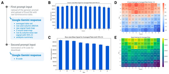
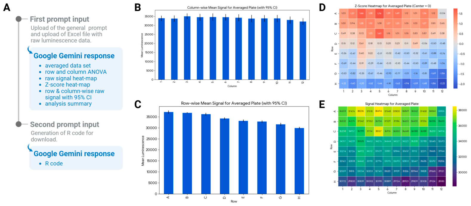
Google Gemini response was composed of three parts (Figure 1). The first part provided detailed analytical reasoning, describing each step of the analysis from data loading and exploration to function definition and report generation. This was followed by a sequence of generated figures which contained raw signal and Z-score heat-maps as well as column-wise and row-wise trend plots, showing mean signals and confidence intervals. The last part was the executive summary and analysis results. Google Gemini provided all the output information requested in the prompt as reviewed in Table 2. Notably, it didn’t suggest any additional prompt ideas or avenues for further analysis beyond those explicitly requested. While no downloadable links to all data (graphics and tables) were provided, each figure was easily downloadable and spreadsheet data exportable into Google sheets. One additional prompt was needed to generate the R-code for download.

Figure 1. Workflow and key results from Google Gemini analysis of the averaged plate dataset. (A) Graphical timeline of user–model interactions, illustrating the sequence of prompt submission and result generation. (B) Column-wise mean luminescence signal with 95% confidence intervals. (C) Row-wise mean luminescence signal with 95% confidence intervals, demonstrating a pronounced top-to-bottom signal gradient. (D) Z-score heatmap for the averaged plate, illustrating standardized deviations across wells; no wells exceeded |Z| > 3.0. (E) Raw luminescence signal heatmap, visualizing the spatial distribution of signal intensity across the 96-well plate.

Google Gemini’s analysis of the four 96-well plates and their average dataset revealed a strong and statistically significant row-wise plate effect. For each plate and the averaged plate, one-way ANOVA produced highly significant p-values for row effects of <0.000001, demonstrating that signal intensity was systematically influenced by row position. Row A consistently exhibited the highest mean signal (averaged plate: 37,099.40), while Row H showed the lowest (averaged plate: 29,864.25), confirming a pronounced edge effect. In contrast, column-wise ANOVA p-values were not significant for any plate (plate 1: p = 0.460404, plate 2: p = 0.271906, plate 3: p = 0.562144, plate 4: p = 0.417925 and averaged Plate: p = 0.764544), indicating no systematic column effect. Subset statistics further supported these findings, with interior wells (rows B–G, columns 2–11) providing a stable baseline and the outer rows deviating markedly. Z-score analysis showed that no wells exceeded the threshold of ∣Z∣ > 3.0, indicating the absence of isolated anomalies. These results were visually corroborated by heatmaps and trend plots, which clearly depicted the spatial signal gradient across rows and the uniformity across columns. Table 3 provides an overview across all four evaluation procedures for easy comparison.

Table 3. Summary of key numerical results obtained from manual and LLM-assisted plate effect analyses (averaged plate dataset). Reported values demonstrate numerical equivalence across analytical approaches.

Metric (Averaged Plate)	Manual (Excel M365)	Google Gemini	ChatGPT	Microsoft Copilot Analyst
Row effect (one-way ANOVA p)	Significant p = 4.31 × 10−37	Significant p < 0.000001	Significant p ≈ 4.3 × 10−37	Significant p < 10−22
Column effect (one-way ANOVA p)	Not significant p = 0.765	Not significant p = 0.765	Not significant p = 0.765	Not significant p ≫ 0.05
Row A mean signal	37,099.4 (95% CI: 36,338.63–37,860.16)	37,099.4 (95% CI: 36,338.63–37,860.16)	37,099.40	37,099.40 (95% CI: 36,338.63–37,860.16)
Row H mean signal	29,864.25 (95% CI: 29,346.80–30,381.70)	29,864.25 (95% CI: 29,346.80–30,381.70)	29,864.25	29,864.25 (95% CI: 29,346.80–30,381.70)
Column 1 mean signal	33,928.47 (95% CI: 32,166.13–35,690.81)	33,928.47 (95% CI: 32,166.13–35,690.81)	(Not explicitly stated)	33,928.47 (95% CI: 32,166.13–35,690.81)
Column 12 mean signal	32,189.78 (95% CI: 29,988.53–34,391.03)	32,189.78 (95% CI: 29,988.53–34,391.03)	(Not explicitly stated)	32,189.78 (95% CI: 29,988.53–34,391.03)
Z-score outliers	No wells with |Z| > 3.0	No wells with |Z| > 3.0	No isolated anomalies by Z-score analysis. Z-score heatmaps confirm absence of extreme outliers.	No isolated anomalies by Z-score analysis. Z-score heatmaps confirm absence of extreme outliers
Spatial autocorrelation (Moran’s I/p)	NA	NA	Moran’s I significant; permutation test p = 0.001	Moran’s I = 0.82
Primary conclusion	Strong row-wise gradient/edge effect, minimal column effect	Same	Same	Same

3.3. ChatGPT Results Overview

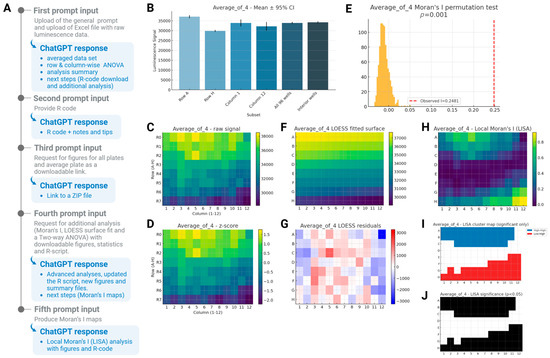
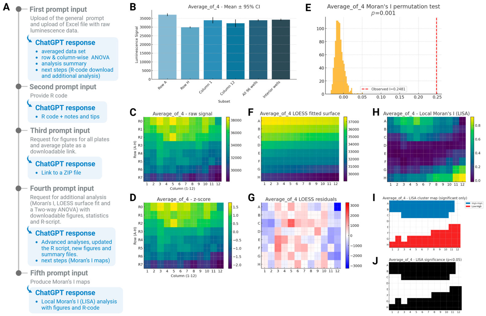
The workflow with ChatGPT was characterized by an interactive, multi-step process rather than a single prompt-and-response exchange. The initial ChatGPT response was composed of two parts. The first part provided a short reasoning step of tool limitations and the provision of both Python-based results and a reproducible R script. This was followed by an overview of analysis performed, files generated, key findings and a list of suggestions for next steps. ChatGPT provided all the output information requested in the prompt, as reviewed in Table 2 including the average signal intensities with 95% CI for rows A and H, columns 1 and 12 as well as all 96 wells and inner 60 wells (Figure 2). No graphics were generated directly in the initial response that would be available for download. However, with additional prompting steps, ChatGPT provided a link to a downloadable ZIP file containing both graphics and any relevant statistical results. Notably, as a result of the first prompt, it suggested additional steps or analyses (such as two-way ANOVA, advanced spatial modeling, and local autocorrelation mapping). Figure 2A displays the multi-step process exchanged with ChatGPT to adapt the analytical scope as proposed by ChatGPT and obtain new figures, tables, and code files tailored to evolving needs.

Figure 2. Overview of the ChatGPT analysis workflow for the averaged plate dataset. (A) Sequence of user prompts and ChatGPT responses, tracing the iterative multi-step analytical process. (B) Mean luminescence signals with 95% confidence intervals for key plate subsets (Row A, Row H, Column 1, Column 12, all 96 wells, and inner 60 wells). (C,D) Heatmaps of raw luminescence signal and Z-scores across the 96-well plate. (E) Moran’s I permutation test result, indicating significant global spatial autocorrelation (p = 0.001). (F,G) LOESS-fitted surface and corresponding residuals, highlighting broad spatial trends and local deviations from the fitted model. (H) Local Moran’s I (LISA) values across the plate. (I) Blue wells (High–High) represent regions with high luminescence surrounded by neighboring wells with similarly high signals, indicating positive local spatial autocorrelation. Red wells (Low–High) represent local spatial outliers with lower-than-average signal surrounded by higher-valued neighboring wells. Wells without significant local spatial autocorrelation are shown in white. (J) Wells exhibiting statistically significant local spatial clustering (black, p < 0.05).

Using the same dataset and prompt, ChatGPT reproduced the same core findings as Gemini, identifying a highly significant row-wise plate effect across all individual plates and the averaged dataset, with no statistically significant column-wise effects. Mean signal intensities for Rows A and H, as well as summary statistics for interior and edge wells, were numerically consistent with those obtained using Google Gemini and the manual analysis (Table 3). Linear spatial modeling further supported these findings, with significant negative row coefficients and minimal column influence. Spatial autocorrelation analyses, including Moran’s I and Local Moran’s I (LISA), revealed systematic gradients along the rows and identified specific wells with significant local spatial clustering, though no isolated anomalies were detected by z-score analysis. These results were visually corroborated by heatmaps, bar plots of mean signals with 95% confidence intervals, and spatial autocorrelation maps.

3.4. Microsoft Copilot Analyst Result Overview

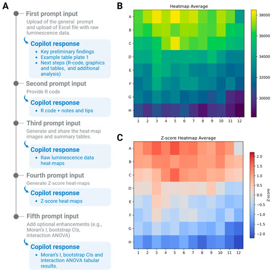
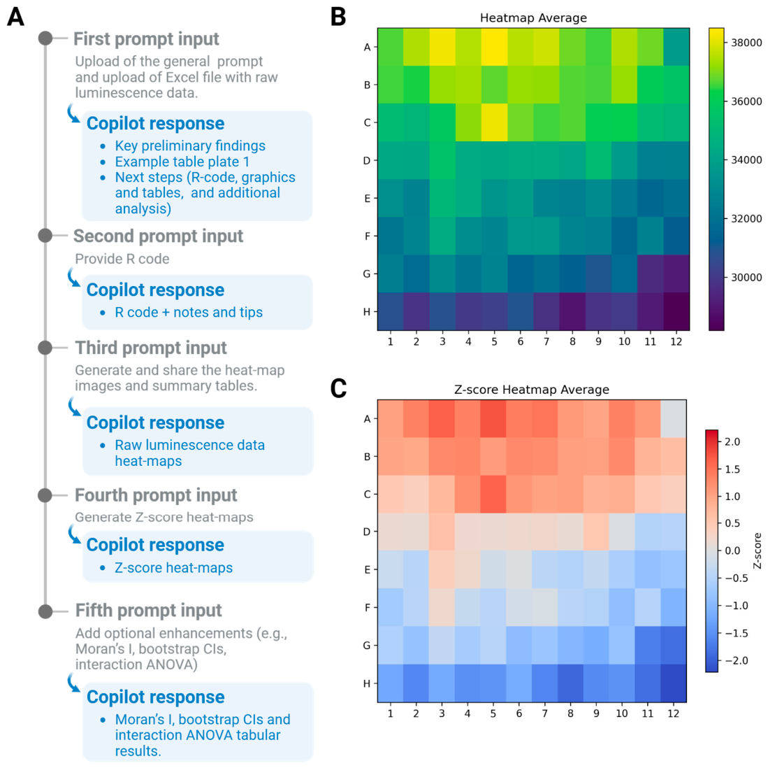
The workflow with Microsoft Copilot Analyst was also characterized by an interactive, multi-step process. The initial Copilot response was short and concise, briefly describing the analyses performed by the R script and key findings of the preliminary analysis. No graphics were provided and the mean raw signal with 95% CI for the different parts of the microtiter plate was calculated for plate 1 only. Copilot did offer three suggestions for next steps which included providing the R code, generating heatmap images and summary tables and additional analysis such as (Moran’s I, interaction ANOVA and bootstrap CIs). With additional prompt, we were able to acquire heatmap images for raw signals and Z-scores as well as tabular data on average raw signal and 95% CI for the different microtiter plate parts, for all four plates and the averaged plate (Figure 3). Additionally, results for Moran’s I, interaction ANOVA and bootstrap CIs were provided by Copilot but only in tabular format. Overview of requested outputs is provided in Table 2.

Figure 3. Overview of the Microsoft Copilot Analyst workflow for the averaged plate dataset. (A) Sequence of user prompts and Copilot Analyst responses, illustrating the iterative prompting steps required to obtain the complete analytical output. (B) Raw luminescence signal heatmap for the averaged plate, visualizing the spatial distribution of signal intensity across the 96-well plate. (C) Corresponding Z-score heatmap, illustrating standardized deviations across wells.

Microsoft Copilot Analyst produced results that were directionally consistent with both Google Gemini and ChatGPT. Across all analyses, Copilot identified the same dominant spatial pattern: higher signals in the upper rows and lower signals toward the bottom of the plate, with minimal column-related variation. Spatial autocorrelation metrics (Moran’s I), provided in tabular form, further supported the presence of clustered spatial structure consistent with a global row effect. Table 3 provides an overview of Copilot Analyst numerical results.

3.5. Manual Plate Effect Analysis Overview

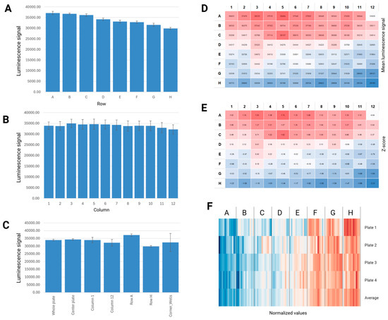
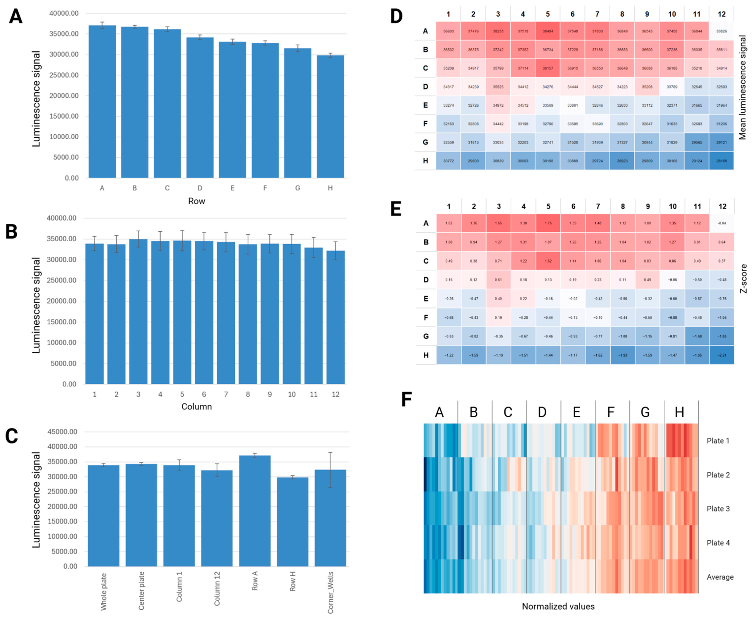
The manual plate effect analysis was performed in Excel for Microsoft 365 (Microsoft Corporation) for each plate and the average dataset. Average raw signal, coefficient of variation (CV) and the 95% confidence interval were calculated for each row, each column, whole plate (96 wells), center plate (60 wells) and corner wells (A1, A12, H1 and H12). Additionally, Z-score and one-way ANOVA were performed for the whole plate and rows and columns respectively. Bar plots of average raw signal with 95% CI and heat-maps of raw signal and z-scores were generated as shown in Figure 4. To show a consistent trend across all plates, each plate was normalized to their individual maximal raw value. These normalized values were then plotted side by side to show a consistent row gradient (Figure 4F).

Figure 4. Overview of the manual plate effect analysis performed in Microsoft Excel for Microsoft 365, shown for the average plate dataset. (A) Row-wise mean luminescence signal (±95% CI), demonstrating a pronounced decreasing gradient from Row A to Row H. (B) Column-wise mean luminescence signal (±95% CI), showing comparatively uniform signal distribution across columns. (C) Mean luminescence signal (±95% CI) for predefined plate regions: entire plate (96 wells), inner wells (60 wells), Row A, Row H, Column 1, Column 12, and corner wells. (D) Heatmap of mean raw luminescence signal across the average plate, where red indicates higher and blue indicates lower luminescence values. (E) Heatmap of Z-scores across the averaged plate, where positive Z-scores are shown in red and negative Z-scores in blue. (F) Stripe plots of normalized raw luminescence data for all four individual plates and the averaged dataset, demonstrating reproducibility of the row-wise signal gradient across plates and analysts; blue indicates below-average and red above-average normalized luminescence values.

Analysis across the four independent plates and the averaged dataset revealed a consistent spatial pattern in signal intensity. Row-wise means exhibited a pronounced gradient, decreasing from the top to the bottom of the plate, with Row A showing the highest average signal (37,099) and Row H the lowest (29,864). In contrast, column-wise averages were comparatively uniform. One-way ANOVA confirmed a robust row effect on every plate (p-values ranging from 1.81 × 10⁻²⁴ to 9.57 × 10⁻²⁷) and in the averaged dataset (p = 4.31 × 10⁻³⁷), whereas no significant effect was detected across columns (p = 0.27–0.76). Taken together, the spatial analysis—summarized by average raw signals (with 95% confidence intervals in the figures) and supported by Z-score-based comparisons—demonstrates a strong row-dependent bias and only minimal column-related variation across plates.

While Table 2 focuses on the availability and type of analytical outputs generated by each model, Table 3 summarizes the corresponding numerical results obtained from the averaged plate dataset. Specifically, Table 3 compiles key statistical metrics—including mean signal intensities, confidence intervals, ANOVA p-values, and spatial analysis outputs—derived from manual analysis and from each LLM-assisted workflow. This table enables direct, side-by-side comparison of calculated values across approaches.

4. Discussion

This study assessed plate homogeneity in a 96-well reporter gene assay dataset, consisting of four independently generated plates, by comparing a manual approach (Excel for Microsoft 365) with three LLM-based analytical workflows (Google Gemini, ChatGPT, and Microsoft Copilot Analyst). In all analyses, one-way ANOVA revealed a consistent and significant row-wise position effect, while column-wise effects were inconsistent and not statistically significant. Notably, the convergence extended beyond significance testing to include consistency in summary statistics (means and 95% confidence intervals calculated for predefined plate regions) and visualization outputs, such as heat maps of raw signals and Z-scores.

While all three LLMs often arrived at the same conclusion, they differed in “how” they supported it. Gemini produced a structured “end-to-end” analysis in one pass, including requested ANOVAs, heatmaps (raw and Z-score), and row/column trend summaries with confidence intervals. Its output closely matched the prompt requirements. Notably, however, Gemini did not proactively expand into additional analyses beyond the explicit request. An approach of this kind is consistent with instruction-following systems tuned to maximize direct compliance and minimize speculative elaboration. Such behavior can reduce the risk of unsupported inferences, a known concern in LLM-generated scientific text and analyses (i.e., “hallucination”), but it may also limit exploratory statistical diagnostics unless explicitly requested [11,12,13,14]. ChatGPT on the other hand met the requested outputs and additionally proposed and, after iterative prompting, delivered more advanced spatial assessment. In particular, spatial autocorrelation methods (e.g., Moran’s I and local indicators) and surface fitting (LOESS) complemented heatmaps by quantifying whether observed patterns depart from spatial randomness and by separating broad spatial trends from local deviations. This is consistent with instruction-aligned models, which often attempt to be maximally helpful by proposing “next steps”. The benefit is that exploratory methods can translate qualitative impressions (“the heatmap is structured”) into quantitative evidence (spatial autocorrelation; modeled trend surfaces). The trade-off, however, is that these expansions require careful verification, e.g., method choice, assumptions and correctness of implementation must be checked to avoid overconfident but incorrect conclusions [11,12,13,14,15,16]. Copilot Analyst initially provided a more minimal response (limited visualization and partial summary calculations) but suggested next steps. With further prompt, it generated the requested heatmaps, Z-scores, and summary tables across all plate regions, and it also pointed toward advanced spatial and inferential extensions (e.g., Moran’s I, interaction ANOVA, bootstrap CIs). This indicates that Copilot can reach comparable depth but may require more iterative steering to achieve a complete analysis package. From a model-level perspective, this pattern is compatible with differences in alignment objectives affecting how much initiative the model takes on first response versus deferring depth until the user confirms scope [13,14].

Overall, the study demonstrates that LLMs can reproduce standard plate analyses and, in some cases, extend beyond typical spreadsheet workflows toward spatial statistics. Importantly, the numerical results reported in Table 3 are effectively identical across all analytical approaches wherever values were explicitly provided. Mean signal estimates, confidence intervals, and statistical conclusions were reproduced consistently by all three LLMs and closely matched the manual Excel-based analysis. These findings reinforce a key conclusion emerging from this comparison: the differences between LLMs were driven less by “fundamental calculations” and more by workflow behavior such as completeness in the first response, degree of exploratory expansion, and the extent of user prompting needed. Gemini and ChatGPT returned more comprehensive first-round outputs aligned with the prompt requirements, whereas Copilot’s first response was comparatively abbreviated and incomplete. In addition, ChatGPT was the most proactive in proposing additional analyses and, after additional interaction, provided deeper spatial diagnostics. Moreover, recent investigations into chain-of-thought behavior indicate that models differ substantially in the transparency and faithfulness of their intermediate reasoning [17,18]. More transparent or reasoning-optimized agents (like Copilot Analyst) behave as iterative problem-solvers that test/refine hypotheses (“more iterative steering”), while front-ends emphasizing concise answers may stay closer to exactly requested outputs (Gemini result). Collectively, these findings underscore that the heterogeneity we observed is not incidental but consistent with well-established model- and system-level differences reported in current scientific research.

An important distinction should be acknowledged when interpreting these findings. The analytical framework applied in this study was largely predefined by the investigators through a structured prompt describing the dataset, analytical objectives, and expected outputs. Consequently, the present work is best viewed as an evaluation of how different LLM systems execute, support, and extend an established analytical workflow rather than a direct assessment of autonomous scientific reasoning. The observed differences between Gemini, ChatGPT, and Copilot primarily reflected variation in workflow behavior, prompt responsiveness, completeness of outputs, and willingness to propose additional analyses, while the underlying statistical framework remained largely defined by the user. Future studies involving more open-ended analytical challenges may provide further insight into the extent to which LLMs can independently formulate, select, and justify analytical strategies.

In addition to the standard statistical methods utilized in this study, the spatial diagnostics recommended by ChatGPT and Copilot—specifically Moran’s I and LOESS surface modeling—offer a scientifically robust extension for assessing microplate heterogeneity. Moran’s I serves as a classical measure of global spatial autocorrelation, quantifying whether adjacent spatial units (in this context, wells) exhibit more similar intensities than would be anticipated under spatial randomness. While sensitive to factors such as the specification of spatial weights and data standardization [19], Moran’s I is widely recognized as an effective tool for identifying spatial clustering across diverse biological datasets, including gene expression, species abundance, cell density, and high-throughput assays [20,21,22,23,24,25]. In our analysis, the significant values observed both across individual plates and on the averaged plate, indicate that the detected spatial pattern corresponds to global positional drift rather than isolated anomalies within specific wells. Two forms of Moran’s I are used in spatial statistics: the global Moran’s I, which provides an overall assessment of whether spatial autocorrelation is present in the entire study area, and the local Moran’s I (LISA), which gives a detailed view of where and how spatial clustering or spatial outliers occur [19]. Local Moran’s I was additionally proposed by ChatGPT to evaluate our data but did not reveal strong local anomalies beyond the global row effect, which aligns with the absence of extreme Z-score outliers. This suggests that while LISA adds granularity, its benefit is likely highest in case of localized artifacts.

LOESS modeling, as introduced by ChatGPT and Copilot, offers a nonparametric technique for fitting smooth spatial trends across the plate surface. Its value lies in its ability to model complex, nonlinear gradients and distinguish broad spatial drift from localized anomalies [26,27]. It has extensive precedent in microarray normalization, where it effectively removes spatial artifacts before differential expression analysis [20,28] and is also used for multi-well plate normalization to minimize plate effects and variability [20,29,30,31]. Given that our dataset exhibited a smooth, monotonic top to bottom gradient consistent across all plates, LOESS is conceptually well suited for describing and correcting such effects. Importantly, however, the current study focuses on diagnostic assessment, not normalization. From a diagnostic standpoint, LOESS helps visualize the underlying spatial surface and confirms that the observed pattern is global and structured, rather than an artifact of random variation.

Overall, these spatial methods complement—rather than replace—the classical analyses and reinforce the interpretation that the dominant plate effect arises from a reproducible, monotonic row trend. Their inclusion demonstrates the potential of LLMs to broaden exploratory statistical assessment while also highlighting the importance of transparent reporting and human verification when applying advanced spatial metrics in bioassay evaluation. Importantly, such integrated spatial assessments go beyond what can be practically implemented using conventional spreadsheet tools, underscoring the added value of LLM-assisted analysis of plate-level effects.

Beyond the analytical findings reported here, one aspect relevant to the practical use of large language models warrants brief clarification. A known characteristic of large language model-based systems is that repeated interactions using identical prompts and input data may not produce exactly identical intermediate outputs or response formulations. This behavior reflects the probabilistic nature of LLM inference and implementation-level factors rather than a change in underlying analytical intent [32,33]. In the present work, we did not specifically design experiments to systematically assess run-to-run reproducibility of LLM outputs, and such an evaluation was therefore outside the formal scope of this study. Nonetheless, during exploratory interactions with the models, we observed that while the structure of generated code, intermediate descriptions, or phrasing of responses could vary between runs, the overarching analytical outcomes and conclusions remained consistent across models and repeated use. Importantly, all core findings reported here are supported by fully reproducible, conventional statistical analyses and manual verification. A formal assessment of reproducibility and stability of LLM-assisted analytical workflows under repeated execution represents an important topic for future methodological studies.

Several limitations of the present study should be considered when interpreting these findings, while also highlighting important directions for future research. The present study was designed as a proof-of-concept comparison rather than a comprehensive validation exercise. Four independent 96-well plates, generated by two analysts on separate days using a single reporter gene assay, were used as a common benchmark dataset for both manual and LLM-assisted analyses. While sufficient to evaluate whether different approaches reached consistent conclusions regarding plate homogeneity, this design does not encompass the full diversity of assay formats, plate densities, detection technologies, or biological systems encountered in bioassay development. Therefore, the findings should be interpreted within the context of the specific real-world analytical dataset evaluated here, rather than as evidence of generalizability across the broader range of bioassay platforms and experimental scenarios encountered in practice.

Furthermore, the evaluated dataset represented a relatively clear and reproducible row-wise spatial gradient that was visually apparent and readily confirmed using conventional statistical approaches. More analytically challenging scenarios—including localized edge effects, mixed spatial artifacts, increased experimental noise, conflicting spatial trends, or intentionally introduced outliers—were outside the scope of the present study. Evaluation of LLM-assisted workflows under such conditions would provide a more rigorous assessment of robustness and generalizability.

Importantly, our conclusions relate specifically to the ability of general-purpose LLMs to reproduce established plate-homogeneity analyses when provided with a structured dataset and clearly defined analytical objectives. They should not be interpreted as a general endorsement of LLM reliability across all analytical applications, nor as evidence that LLMs can replace scientific expertise and statistical oversight. Rather, the observed agreement between manual analysis and the outputs generated by Google Gemini, ChatGPT, and Microsoft Copilot Analyst suggests that these tools may serve as useful analytical companions for well-defined quality-control tasks when their outputs are reviewed by trained scientists. Future studies should evaluate larger datasets, multiple assay formats, more complex spatial artifacts, and additional laboratories to determine the generalizability, robustness, and reproducibility of LLM-assisted analytical workflows.

5. Conclusions

Within the scope of the reporter gene assay dataset evaluated in this study, all tested general-purpose LLMs successfully reproduced the results of conventional plate-homogeneity analyses and identified the same dominant row-wise spatial bias as the manual reference workflow. Differences between models were observed primarily in workflow behavior, prompt responsiveness, analytical completeness, and the extent of additional exploratory analyses proposed rather than in the final statistical conclusions. While additional validation using more complex datasets, assay formats, and experimental conditions is warranted, these findings suggest that general-purpose LLMs can serve as useful analytical companions for well-defined microplate quality-control tasks when applied with structured prompts, complete datasets, and appropriate scientific oversight.

References

- Wouters, O.J.; McKee, M.; Luyten, J. Estimated Research and Development Investment Needed to Bring a New Medicine to Market, 2009–2018. JAMA-J. Am. Med. Assoc. 2020, 323, 844–853. [Google Scholar] [CrossRef] [Scilit] [PubMed]
- Zheng, Y.; Koh, H.Y.; Ju, J.; Yang, M.; May, L.T.; Webb, G.I.; Li, L.; Pan, S.; Church, G. Large language models for drug discovery and development. Patterns 2025, 6, 101346. [Google Scholar] [CrossRef] [Scilit] [PubMed]
- Othman, Z.K.; Ahmed, M.M.; Okesanya, O.J.; Ibrahim, A.M.; Musa, S.S.; Hassan, B.A.; Saeed, L.I.; Lucero-Prisno, D.E. Advancing drug discovery and development through GPT models: A review on challenges, innovations and future prospects. Intell. Based Med. 2025, 11, 100233. [Google Scholar] [CrossRef] [Scilit]
- Kant, S.; Deepika; Roy, S. Artificial intelligence in drug discovery and development: Transforming challenges into opportunities. Discov. Pharm. Sci. 2025, 1, 7. [Google Scholar] [CrossRef] [Scilit]
- Lu, J.; Choi, K.; Eremeev, M.; Gobburu, J.; Goswami, S.; Liu, Q.; Mo, G.; Musante, C.J.; Shahin, M.H. Large Language Models and Their Applications in Drug Discovery and Development: A Primer. Clin. Transl. Sci. 2025, 18, e70205. [Google Scholar] [CrossRef] [Scilit] [PubMed]
- Zheng, Y.; Koh, H.Y.; Yang, M.; Li, L.; May, L.T.; Webb, G.I.; Pan, S.; Church, G. Large Language Models in Drug Discovery and Development: From Disease Mechanisms to Clinical Trials. arXiv 2024, arXiv:2409.04481. [Google Scholar]
- Liao, Q.; Zhang, Y.; Chu, Y.; Ding, Y.; Liu, Z.; Zhao, X.; Wang, Y.; Wan, J.; Ding, Y.; Tiwari, P.; et al. Application of Artificial Intelligence in Drug-target Interactions Prediction: A Review. npj Biomed. Innov. 2025, 2, 1. [Google Scholar] [CrossRef] [Scilit] [PubMed]
- White, J.R.; Abodeely, M.; Ahmed, S.; Debauve, G.; Johnson, E.; Meyer, D.M.; Mozier, N.M.; Naumer, M.; Pepe, A.; Qahwash, I.; et al. Best practices in bioassay development to support registration of biopharmaceuticals. Biotechniques 2019, 67, 126–137. [Google Scholar] [CrossRef] [Scilit] [PubMed]
- Singh, R.; Maheshwari, P. Evaluation of plate edge effects in in-vitro cell based assay. Int. J. Latest Trans. Eng. Sci. 2019, 7, 52–57. [Google Scholar]
- Lundholt, B.K.; Scudder, K.M.; Pagliaro, L. A simple technique for reducing edge effect in cell-based assays. J. Biomol. Screen 2003, 8, 566–570. [Google Scholar] [CrossRef] [Scilit] [PubMed]
- Nori, H.; King, N.; McKinney, S.M.; Carignan, D.; Horvitz, E. Capabilities of GPT-4 on Medical Challenge Problems. arXiv 2023, arXiv:2303.13375. [Google Scholar]
- Ji, Z.; Lee, N.; Frieske, R.; Yu, T.; Su, D.; Xu, Y.; Ishii, E.; Bang, Y.J.; Madotto, A.; Fung, P. Survey of Hallucination in Natural Language Generation. ACM Comput Surv. 2023, 55, 1–38. [Google Scholar] [CrossRef] [Scilit]
- Wei, J.; Bosma, M.; Zhao, V.Y.; Guu, K.; Yu, A.W.; Lester, B.; Du, N.; Dai, A.M.; Le, Q.V. Finetuned Language Models Are Zero-Shot Learners. arXiv 2022, arXiv:2109.01652. [Google Scholar]
- Ouyang, L.; Wu, J.; Jiang, X.; Almeida, D.; Wainwright, C.; Mishkin, P.; Zhang, C.; Agarwal, S.; Slama, K.; Ray, A.; et al. Training language models to follow instructions with human feedback. Adv. Neural Inf. Process. Syst. 2022, 35, 27730–27744. [Google Scholar] [CrossRef] [Scilit]
- Tabassi, E. Artificial Intelligence Risk Management Framework (AI RMF 1.0); National Institute of Standards and Technology: Gaithersburg, MD, USA, 2023. [CrossRef] [Scilit]
- Maynez, J.; Narayan, S.; Bohnet, B.; McDonald, R. On Faithfulness and Factuality in Abstractive Summarization. In Proceedings of the 58th Annual Meeting of the Association for Computational Linguistics; Association for Computational Linguistics: Stroudsburg, PA, USA, 2020; pp. 1906–1919. [Google Scholar] [CrossRef] [Scilit]
- Hebenstreit, K.; Praas, R.; Kiesewetter, L.P.; Samwald, M. A comparison of chain-of-thought reasoning strategies across datasets and models. PeerJ Comput. Sci. 2024, 10, e1999. [Google Scholar] [CrossRef] [Scilit] [PubMed]
- Chen, Y.; Benton, J.; Radhakrishnan, A.; Uesato, J.; Denison, C.; Schulman, J.; Somani, A.; Hase, P.; Wagner, M.; Roger, F.; et al. Reasoning Models Don’t Always Say What They Think. arXiv 2025, arXiv:2505.05410. [Google Scholar]
- Bivand, R.S.; Pebesma, E.; Gómez-Rubio, V. Applied Spatial Data Analysis with R; Springer: New York, NY, USA, 2013. [Google Scholar] [CrossRef] [Scilit]
- Lachmann, A.; Giorgi, F.M.; Alvarez, M.J.; Califano, A. Detection and removal of spatial bias in multiwell assays. Bioinformatics 2016, 32, 1959–1965. [Google Scholar] [CrossRef] [Scilit] [PubMed]
- Schmal, C.; Myung, J.; Herzel, H.; Bordyugov, G. Moran’s I quantifies spatio-temporal pattern formation in neural imaging data. Bioinformatics 2017, 33, 3072–3079. [Google Scholar] [CrossRef] [Scilit] [PubMed]
- León, F.; Pizarro, E.; Noll, D.; Pertierra, L.R.; Parker, P.; Espinaze, M.P.A.; Luna-Jorquera, G.; Simeone, A.; Frere, E.; Dantas, G.P.M.; et al. Comparative genomics supports ecologically induced selection as a putative driver of banded penguin diversification. Mol. Biol. Evol. 2024, 41, msae166. [Google Scholar] [CrossRef] [Scilit] [PubMed]
- Dávid, C.; Giber, K.; Kerti-Szigeti, K.; Kollo, M.; Nusser, Z.; Acsády, L. An image segmentation method based on the spatial correlation coefficient of Local Moran’s I—Identification of A-type potassium channel clusters in the thalamus. eLife 2023, 12, RP89361. [Google Scholar] [CrossRef] [Scilit]
- Emons, M.; Gunz, S.; Crowell, H.L.; Mallona, I.; Kuehl, M.; Furrer, R.; Robinson, M.D. Harnessing the potential of spatial statistics for spatial omics data with pasta. Nucleic Acids Res. 2025, 53, gkaf870. [Google Scholar] [CrossRef] [Scilit] [PubMed]
- Malo, N.; Hanley, J.A.; Cerquozzi, S.; Pelletier, J.; Nadon, R. Statistical practice in high-throughput screening data analysis. Nat. Biotechnol. 2006, 24, 167–175. [Google Scholar] [CrossRef] [Scilit] [PubMed]
- Cleveland, W.S. Robust Locally Weighted Regression and Smoothing Scatterplots. J. Am. Stat. Assoc. 1979, 74, 829–836. [Google Scholar] [CrossRef]
- Hastie, T.; Tibshirani, R.; Friedman, J. The Elements of Statistical Learning; Springer: New York, NY, USA, 2009. [Google Scholar] [CrossRef]
- Smyth, G.K.; Speed, T. Normalization of cDNA microarray data. Methods 2003, 31, 265–273. [Google Scholar] [CrossRef] [Scilit] [PubMed]
- Fang, R.; Wey, A.; Bobbili, N.K.; Leke, R.F.G.; Taylor, D.W.; Chen, J.J. An analytical approach to reduce between-plate variation in multiplex assays that measure antibodies to Plasmodium falciparum antigens. Malar. J. 2017, 16, 287. [Google Scholar] [CrossRef] [Scilit] [PubMed]
- Hong, M.-G.; Lee, W.; Nilsson, P.; Pawitan, Y.; Schwenk, J.M. Multidimensional Normalization to Minimize Plate Effects of Suspension Bead Array Data. J. Proteome Res. 2016, 15, 3473–3480. [Google Scholar] [CrossRef] [Scilit] [PubMed]
- Wu, L.; Hall, T.; Ssewanyana, I.; Oulton, T.; Patterson, C.; Vasileva, H.; Singh, S.; Affara, M.; Mwesigwa, J.; Correa, S.; et al. Optimisation and standardisation of a multiplex immunoassay of diverse Plasmodium falciparum antigens to assess changes in malaria transmission using sero-epidemiology. Wellcome Open Res. 2020, 4, 26. [Google Scholar] [CrossRef] [Scilit] [PubMed]
- Yang, H.; Zhao, Y.; Wu, Y.; Wang, S.; Zheng, T.; Zhang, H.; Ma, Z.; Che, W.; Wang, S.; Wei, S.; et al. Large language models meet text-centric multimodal sentiment analysis: A survey. Sci. China Inf. Sci. 2025, 68, 200101. [Google Scholar] [CrossRef] [Scilit]
- Herrera-Poyatos, D.; Peláez-González, C.; Zuheros, C.; Herrera-Poyatos, A.; Tejedor, V.; Herrera, F.; Montes, R. An overview of model uncertainty and variability in LLM-based sentiment analysis: Challenges, mitigation strategies, and the role of explainability. Front. Artif. Intell. 2025, 8, 1609097. [Google Scholar] [CrossRef] [Scilit] [PubMed]
Disclaimer/Publisher’s Note: The statements, opinions and data contained in all publications are solely those of the individual author(s) and contributor(s) and not of MDPI and/or the editor(s). MDPI and/or the editor(s) disclaim responsibility for any injury to people or property resulting from any ideas, methods, instructions or products referred to in the content. |
© 2026 by the authors. Licensee MDPI, Basel, Switzerland. This article is an open access article distributed under the terms and conditions of the Creative Commons Attribution (CC BY) license.