


Abstract
Accurate and efficient computation of partial inductances is essential in modern electromagnetic modeling. A three-dimensional cubic spline interpolation method is proposed for efficient evaluation of partial inductances between uniform cubic cells on a Cartesian grid, a common configuration in FFT-accelerated methods, including PEEC. The interpolation dimensionality is chosen to match the three-dimensional nature of the problem. Two reference grid types are investigated: a uniform Cartesian grid and a nonuniform grid with predominantly logarithmic spacing. The results show that the uniform grid does not provide sufficient accuracy in the near region under practical memory constraints, whereas the nonuniform logarithmic grid, augmented with a point at zero, enables accurate evaluation over the entire problem space. The interpolation error is controlled by the number of reference points per decade and the interpolation order, providing a trade-off between accuracy and computational cost. The influence of boundary effects is also analyzed, confirming that they can affect interpolation accuracy and should be considered in practical applications. Simulation results demonstrate that the proposed method achieves maximum relative errors down to approximately 10−7 with practical memory configurations. It provides accuracy comparable to Tucker reconstruction while offering about 30× faster usage-phase evaluation. In addition, it improves accuracy over one-dimensional spline interpolation while maintaining comparable evaluation speed.
1. Introduction
Electrical and electronic systems nowadays are present in all aspects of our lives. Almost all devices that we use today are dependent on electricity, and most of them rely on electronics to perform their functions. The road from idea to a customer-ready device or system roughly follows the design, prototype, and final product phases [1]. The prototype phase may be too costly, especially for more complex devices, where several cycles of prototyping may be needed. With the advancement of computers, simulation is one of the indispensable tools that help reduce or even avoid the physical prototyping phase [2], leading to a faster and more affordable product development cycle.
In the field of electrical and electronics engineering, simulation tools that can simulate a broad family of different types of circuits, with different types of electrical and electronics components, are broadly known as SPICE (Simulation Program with Integrated Circuit Emphasis) [3]. SPICE accepts a circuit description, with several components, sometimes thousands or millions of them, and information about the interconnection between them. Then, simulations of different scenarios can be performed, with the aim of predicting and determining whether the design fulfills requirements. Each type of physical component, or a similar group of them, is represented with a sort of model that describes its behavior, sometimes with more and sometimes with less detail [4]. The complexity of the model is a kind of trade-off between the accuracy of description and the speed of simulation. A physical counterpart to these simulations for small- to moderate-size circuits could be breadboarding [5]. SPICE simulation assumes that interconnections are ideal and, besides connecting or shorting two or more component terminals to a single node, have no other physical or electrical properties. A similar assumption is often made during breadboard prototyping, where the type of wire that we use (length, thickness, isolation, form) is dictated more by the practical issue of making a connection between desired points than by considering the realistic electrical parameters they introduce in the circuit [5]. SPICE also assumes lumped parameter models for components [4], i.e., their physical size is negligible, and each is considered as a point.
With ever-increasing working speed and frequency for devices under test, the lumped parameter assumption does not hold anymore. In widespread electrical systems or interconnected electronic systems, even very low working frequencies, like 50 Hz in power distribution [6] or 300 Hz to 3400 Hz in wired telephony [7], may require more elaborate models for interconnections that treat them as distributed parameter parts of the system. This necessity, especially at working frequencies in the GHz range and with very short rise and fall times, extends to PCBs (Printed Circuit Boards) [5,8], component packages and internal wiring [9], and even inner parts of components [10], such as integrated circuit dies. Some aspects of accounting for physical dimensions are also present in certain component models in SPICE [4], where they are used for estimating parasitic effects.
When distributed parameters dominate the problem, SPICE is no longer the appropriate tool to solve it. Other numerical tools for electromagnetic problems are more commonly used. Since many design problems involve common electrical and electronic components, while at the same time the nature of the problems demands distributed parameter treatment, sometimes referred to as electromagnetic circuit problems, tools that can handle both aspects are needed [11]. The partial element equivalent circuit (PEEC) method [12,13] was developed with the aim of keeping SPICE as a common circuit solver tool by converting the electromagnetic part with distributed parameter modeling requirements into a SPICE-friendly form.
Many numerical methods for solving electromagnetic problems, including the PEEC method, discretize or mesh the problem space into many small regular cells during one of the simulation steps [14]. The PEEC method has a developed strategy to build an equivalent circuit for each cell with common electrical components: resistors, inductors, and capacitors. Schematics for cells are defined by the method and are dependent on the type of material for that specific cell [13], being a conductor, dielectric, or magnetic material. These partial models are SPICE-friendly and can be easily included alongside other lumped circuit components. A neighborhood with other touching cells dictates interconnections between partial models. The PEEC method is based on the integral form of Maxwell’s equations and needs to mesh only material space, and not free space. Magnetic and electric field couplings between cells are represented by mutual inductances and coefficients of potential, mostly implemented in the model by SPICE-controlled sources [4,15]. Components used to build the PEEC model are known as partial elements [12]. All couplings are grouped into the off-diagonal elements of two dense matrices—the partial inductance matrix Lp and the matrix of coefficients of potential Pp—while diagonal elements contain self-partial elements. A third matrix, R, contains partial resistances. This work focuses on improving the efficiency and accuracy of evaluating these coupling terms in large-scale discretized domains, which represents one of the major computational bottlenecks in PEEC-based simulations.
While the structure of the PEEC model is stereotypical for every problem, the computationally expensive part is composing system equations with specific values for self-components of each cell and values for mutual couplings between cells, i.e., matrices Lp, Pp, and R [16]. The complexity of these calculations is directly related to the geometry of the cell and the equations that these calculations are based on. Self and mutual magnetic couplings Lp(i,j) require the solution of sixfold integrals, while electric couplings Pp(i,j) require the solution of quadruple integrals, where the first one is considered the most time-consuming [17]. The general preference for the PEEC method is to use a Manhattan type of meshing that results in parallelepiped cells [16]. One of the reasons for this preference is the existence of analytic formulas for calculating values of partial elements [16,18], for both self and mutual. Another reason is the possibility of using very high aspect-ratio cells. In general cases, for other shapes of the cells (non-orthogonal, cylindrical), evaluation of partial elements is performed by numerical integration, mostly by the Gaussian quadrature [17,19].
To make computation of partial elements using numerical integration more efficient, compared to the standard adaptive method with given maximum error, one approach was to identify different zones where a specific order of Gauss–Legendre quadrature is required to achieve desired accuracy [20,21]. This puts adaptive parts of processing at a noncritical time, and one order-k Gauss–Legendre quadrature would be used for a single partial element belonging to the order-k zone. This resulted in orders of magnitude speedup with acceptable accuracy. Since one must deal with higher-order numerical integration, zones may have different combinations of integration orders for each separate dimension. This strategy effectively shifts computational effort into a preprocessing stage, improving runtime performance for repeated evaluations.
Another approach to improving computational efficiency combines analytical and numerical methods, where analytical expressions are used for selected dimensions and Gaussian quadrature is applied to the remaining ones. In one formulation for partial inductance computation [17,19], analytical expressions for mutual inductance between parallel filaments reduce the numerical integration order from six to four, significantly decreasing computational cost while improving both accuracy and speed.
Fully analytic formulas for partial inductance computation, as a preferred choice for the PEEC method, exist for orthogonal cases [13,18]. They cover the situations where cells are of rectangular parallelepiped shape, and the mutual position between cells should have faces parallel to each other. All this is based on the generally accepted assumption of constant current density over the whole cell, with the current direction assumed to be parallel to the cell axis [22]. This configuration results in only one non-zero situation, when currents in both cells (for mutual partial inductances) are parallel. Other possibilities for current direction, under the mentioned assumptions, are with orthogonal current directions. These situations result in a zero-valued integral, and no corresponding partial elements will be included in the model. These analytical formulas proved to be very sensitive to finite precision of number representation, with double precision floating-point format (IEEE 754 binary64, or double-precision) considered standard nowadays, due to the subtraction of numbers with similar magnitudes, where an enormous loss of significant digits may happen [18,22]. When one or more dimensions become small relative to the others, the evaluation of the analytical formula will lose several significant digits, up to the point of producing numerically meaningless results. To overcome this situation and keep the error under control, an approach with multiple analytic functions was used [22,23], with switching to the most appropriate one depending on the set of conditions in the function of cell sizes in each direction and the distance between them. Individual cells are categorized as volume, surface, line, or point type, and all combinations between two of these types can be present when the mutual interaction between two cells is considered, i.e., volume-volume, volume-surface, up to the simplest case of point–point interaction. For all possible combinations, a set of analytical formulas was derived. Currently, the method in [22] can be considered a reference for the general orthogonal case in terms of accuracy and speed. The most popular filament–filament approximation formula [18,22] is included in this set as the line–line type.
Recent improvements in the PEEC method and in the standard Volume Integral Equation (VIE) method are to use Fast Fourier Transform (FFT) and Inverse Fast Fourier Transform (IFFT) to speed up matrix-vector multiplication [24,25]. In its standard implementation, it requires the discretization to be uniform, separately in each space dimension, with the size of all cells equal to dx, dy, and dz in corresponding directions. When the problem space is extended into three dimensions and FFT-acceleration is used, the same discretization in all three dimensions can be used, with dx = dy = dz, where the problem space is discretized with a uniform grid of cubic cells [24,26]. With a uniform grid, be it with cubic cells or with parallelepiped cells, and based on a feature that the magnetic coupling matrix has in this special case, only one row of the inductance matrix must be computed. Even the standard, non-FFT-accelerated PEEC method [16] can benefit from cubic cells since they are computationally more efficient.
For discretization with uniform cubic cells, an extreme approach is to precompute mutual couplings for all possible combinations of cell positions with desired accuracy, usually assuming a normalized cell size and the maximal problem space. The calculation of a single partial element in this case would consist of only one indexed reading from a three-dimensional (3D) matrix, but the size of the corresponding matrix can be huge. To reduce memory requirements, a compressed version of this matrix with Tucker decomposition is used, which is the most popular approach [27,28]. A similar approach has been used in the VIE method [27] and in general inductance [26] and capacitance solvers [29].
One recent approach for the computation of partial inductances and partial coefficients of potential for cubic cells is to use interpolation [30,31,32]. It computes couplings using one-dimensional (1D) cubic spline interpolation over center-to-center distance, Rcc, from two sets of a small number of couplings at selected distances, for near and far zones [31,32]. Couplings at logarithmically spaced distances are selected from all pairs of cells sorted by distance Rcc. Couplings at selected distances are computed with the multiple analytic functions method [22]. For other intermediate distances, partial elements are computed by cubic spline interpolation. Interpolation has also been used for fast frequency sweep between PEEC models at several selected points [33].
Despite analytical, numerical, and decomposition-based approaches for evaluating partial inductances, existing methods have limitations in large-scale FFT-compatible discretization. Analytical formulations can become computationally expensive or numerically unstable for general geometries. 1D interpolation reduces cost and memory usage but does not preserve the three-dimensional (3D) structure, which may reduce accuracy in regions with strong spatial variation. Tucker-based approaches provide accurate reconstruction but remain computationally expensive per evaluation due to tensor operations and memory accesses. The proposed 3D interpolation framework targets accuracy comparable to Tucker reconstruction while maintaining a computational cost per evaluation closer to 1D interpolation in the usage phase. It uses 3D interpolation on structured Cartesian grids with precomputed reference values, reducing arithmetic operations and memory accesses relative to Tucker methods. Accuracy is controlled through grid type, grid resolution, interpolation order, and mitigation of boundary effects. Preprocessing is a one-time cost and does not affect repeated evaluations. The same considerations apply to standard PEEC formulations using Cartesian discretization.
Cubic-cell-based meshing with centers on a 3D Cartesian grid is a commonly used configuration for FFT-accelerated methods, including FFT-accelerated variants of the PEEC method. When normalized cubic cells are used, evaluation of mutual partial inductances is inherently a 3D problem. While all methods for the evaluation of mutual partial inductance between parallelepiped cells can be applied [22], more efficient evaluation can be achieved by exploiting the lower dimensionality of the problem. Two more recent methods with this approach are Tucker reconstruction [28] and cubic spline interpolation [31]. The former enables a high compression ratio for storing precomputed partial elements, requiring much less memory compared to the original inductance matrix. The standard version of this method uses the full inductance matrix during the preparatory phase and decomposes it into four matrices, resulting in a much more compact representation for the desired accuracy. Reconstruction of accurate original data, when needed, can usually be performed faster than direct computation with similar accuracy. The preparatory phase may be time-consuming, but it is performed only once. The latter method [31] uses a small set of original partial inductance values and computationally reconstructs values over the entire domain covered by the original data using 1D cubic spline interpolation. This set is much smaller than the full set used in Tucker decomposition. In addition, computing values at arbitrary query points is less computationally expensive than in the Tucker approach. However, the interpolation method in [31], while fast and memory-efficient, exhibits low accuracy in near and far regions, with somewhat better accuracy in the intermediate region. This behavior may primarily result from interpolating 3D data using 1D interpolation, the number and distribution of sampled points, and unhandled boundary effects.
In this paper, we investigate the accuracy and computational characteristics of 3D interpolation for evaluating mutual partial inductances between reference cubic cells on a 3D Cartesian grid, where the interpolation dimensionality matches the 3D nature of the problem. For this 3D interpolation method, two reference grid types are considered: a uniform Cartesian grid and a nonuniform (mostly) logarithmic grid, identical in each of the three spatial dimensions. Another parameter considered is the interpolation order. While it is intuitive that increasing the number of points and the order of interpolation will decrease interpolation error, this paper aims to provide guidelines for the selection of interpolation parameters for a given partial inductance accuracy and the resulting computational and memory requirements needed to achieve it. Usually, the selection is a trade-off among three factors, namely accuracy, computational time, and memory resources. We also show how untreated boundary effects influence the error and how to mitigate them. An additional aspect of interpolation analyzed is the distinction between calculations performed during the preparatory phase and those performed during the usage phase. The paper continues with a presentation of the partial inductance calculation problem for orthogonal cases and computational methods used to generate reference points for accuracy estimation and interpolation.
2. Materials and Methods
2.1. Partial Self and Mutual Inductance Between Rectangular Cells
Mesh-based numerical methods, where the PEEC method belongs, discretize problem geometry into a set of elementary cells [30]. In general, these cells can be of any shape, but in practical applications, they belong to a narrow group of shapes. Manhattan meshing, considered standard meshing for the PEEC method [16], consists of rectangular parallelepiped-shaped cells with faces parallel to coordinate system planes. When the discretization is uniform along all three axes, all cells will be of the same size and may be either parallelepipeds or cubes. Uniform discretization is typically required for applying FFT-acceleration [25]. In the following paragraphs, we will assume uniform discretization on a Cartesian grid. Although a general rectangular parallelepiped (cuboid) discretization of dimensions N1 × N2 × N3 is possible, in this work, we adopt a cubic reference configuration N × N × N, where N = max(N1, N2, N3), ensuring that all cuboid problem spaces can be embedded into a common reference domain. This choice aligns the formulation with representative configurations used in the literature [31,32] and provides a unified indexing framework for the evaluation of partial inductances based on relative cell distances. Cells will be cubic with a reference size of 1 m in each of three dimensions. We adopt a problem space composed of regularly arranged 1001 × 1001 × 1001 cubic cells, with centers located at the integer-distance positions, starting from zero, for each of the coordinates [31,32]. The problem space of a smaller size is shown in Figure 1. Some of these cells may contain conductive, dielectric, or magnetic material, whereas the remaining cells correspond to air [25]. In standard volume-based PEEC formulations [13], partial mutual inductances are evaluated between cells carrying equivalent currents, regardless of whether these currents originate from conduction, displacement, or magnetization effects. In FFT-accelerated PEEC formulations [24,25], the same evaluation procedure is additionally extended to the entire computational domain, including air cells, due to the regular grid structure required for FFT-based acceleration. In all such cases, the same underlying partial inductance expressions are used to evaluate the corresponding interaction terms, enabling a unified treatment of the considered interpolation and acceleration methods independently of the specific material distribution within the problem space.
Figure 1.
Problem space of size 10 × 10 × 10 cubic cells. Two conductive bodies, the first containing cell 1 and the second containing cell 2, are meshed with cubic cells. Green and red cubes correspond to the representative cell pair obtained after applying translation invariance to cells 1 and 2. This translation-invariant representation reduces the number of unique partial inductance configurations that must be evaluated. In the case of standard PEEC, only conductors are meshed [12,13], while for FFT-accelerated PEEC, the entire problem space, including air, is meshed [25].
When computing mutual inductance between two cells anywhere in the problem space, cell 1 and cell 2 in Figure 1, we can always assume that the center of the first cell is located at the origin of the coordinate system (0, 0, 0), the green cell, while the center of the second cell is located at position (|x1 − x2|, |y1 − y2|, |z1 − z2|), where each coordinate assumes an integer value. The situation with both cells at the origin corresponds to self-partial inductance. This setup covers all possible combinations inside a problem space, since the free-space Green’s function is translation-invariant [32]. For cell sizes different from the reference cell size, a dimensionless scaling factor is applied to obtain the final values of partial mutual inductances from the reference values [31].
Evaluating each element of the partial inductance matrix (Lp) requires the solution of a six-dimensional integral over two volumes. In the case of rectangular parallelepiped or cubic cells, under the quasi-static assumption and uniform current density over the cell cross-section, these integrals simplify to the following form [18]:
where Vm and Vn are cell volumes, Rmn is the distance between two points, one located inside cell m and the other inside cell n, and Sm and Sn are cross-sections normal to the current directions in volumes Vm and Vn, respectively.
The integral in (1), under the given assumptions, has a closed-form solution. Derivation of the solution can be found in [18,34], while the final version can also be found in [22]. For the sake of completeness, we include the result in this paper. Mutual partial inductance between cell 1 and cell 2 is expressed as a sum of 64 similar functions:
where W1, T1, W2, and T2 are cell width and cell thickness for cells 1 and 2, respectively, and qi, rj, sk are limits of integration [18,34]. The expression for the function is:
Proper handling of (3) during computation to avoid singularities and assure evaluation in the proper quadrant is described in [22]. The computation of partial mutual inductances that will be used as reference values is based on Equations (2) and (3).
For partial self-inductance, one can also use (2) and (3), or other closed-form solutions tailored for self-inductance, such as the Ruehli [35] or FastHenry [36] formulas. For problems that use a regular Cartesian mesh, be it with rectangular parallelepiped or cubic cells, all cells will be of the same shape and dimension, and there will be only one partial self-inductance for all of them. In such cases, the corresponding value is calculated only once, and the stored value is reused thereafter. For cubic cells, the stored partial self-inductance of the reference cube is used, followed by appropriate scaling to the actual cube size.
2.2. Evaluation of Closed-Form Solution Using Double-Precision Arithmetic
Double-precision floating-point format (IEEE 754 binary64) is considered standard nowadays and provides about 15.95 significant digits. Processors and different mathematics-intensive software are usually optimized using double-precision operations. The closed-form solution, Equations (2) and (3), covers all possible configurations under the given assumptions and would be a preferred choice for any application. For cubic cells far apart, values of function f (x, y, z) will grow with about the fifth power of distance. When cell size starts to become small relative to the distance, values of function f will be very close to each other. Differences between these values evaluated with double precision, as in (2), will result in an increasing loss of significant digits with increasing distance between cells [22], up to a point of producing numerically meaningless values for computed mutual inductances.
It is this accuracy degradation in double-precision evaluation of closed-form solutions that has led to the development of other methods that avoid extreme cancellation through different approaches [22]. However, for relatively comparable cell sizes and distances between them, it is still mostly used, with numerical methods such as Gaussian quadrature being another option [37].
2.3. Evaluation of Closed-Form Solution Using Variable-Precision Arithmetic
When there is a closed-form solution, but its performance is degraded in finite-precision arithmetic because of ill-conditioned expressions, one can relax the problem to an acceptable point by using more accurate digits. One possibility of achieving this is to use variable-precision arithmetic (VPA), where hundreds or thousands of accurate digits can be selected. In our case, we need enough accurate digits when evaluating (2) and (3) to provide a result with maximum or other selected accuracy in double precision when it is converted from VPA to double [18,38].
Reference values, used to assess the performance of other methods for computing partial inductances, are evaluated using variable-precision arithmetic with 64 significant digits and will be referred to briefly as VPA64. For problem sizes and mesh resolutions [22] used for illustration, the number of significant digits starting from around 32 and above provided sufficiently accurate values, while no noticeable difference in computation time was observed; 64 were selected for plenty of guard digits, in addition to the internal ones. They provide maximum machine precision when VPA64 values are converted to double, either for validation of other methods or as preprocessed reference values in other methods for further processing.
2.4. Dimensionality of Partial Inductance Computation and Tabular Approach
Computation of mutual partial inductances of rectangular parallelepiped-shaped cells with faces parallel to coordinate system planes, resulting from Manhattan meshing, is a 9-dimensional problem [18]. The dimensionality of the problem reduces to three when both cells are cubes of the same normalized size, with these three dimensions being the distances between cells in three directions. When the positions of the cells are constrained to a uniform Cartesian grid with a limited range in each of the three directions, the problem becomes discrete and reduces further to a finite number of states [31,32]. As mentioned in one of the previous sections, since the free-space Green’s function is translation invariant, the number of states reduces to N1 × N2 × N3, where Ni is the number of cells along the i-th dimension, or N3, assuming the number of cells is the same in all three dimensions, without loss of generality for the considered class of uniform Cartesian discretizations.
For a wide range of N, limited only by available memory, a pure tabular approach can be used as an alternative to computing values during the usage phase. For a problem space with N = 1001, comparable in size to the problems considered in [31,32], and for each value represented with double precision, storing a table of precomputed partial inductance values would require about 8 GB (gigabytes) of memory. The value stored at position (0, 0, 0) (assuming 0-based indexing) would correspond to the partial self-inductance, while other values would correspond to mutual terms. For the new method, only a subset of this table will be used for validation or as reference values for other methods.
To find the partial mutual inductance between two given cubic cells with coordinates (x1, y1, z1) and (x2, y2, z2), where xi, yi, and zi are integers with values in the range from 0 to N−1, the relative distances in all three directions will define the query point:
The stored value at position (xq, yq, zq) corresponds to the partial mutual inductance between the two given cubic cells. When distances are used for indexing purposes, they are assumed to be integer-valued and dimensionless quantities. In the following, we will assume that the relative distances are given instead of individual cell coordinates.
This would provide fast and highly accurate “computed” values for partial inductances using a tabular approach. The speed would be comparable to that of random reads from main memory, whereas the accuracy would depend on the method used to precompute the table entries.
For the highest accuracy, limited only by machine precision, VPA64 will be used. When less accurate values are sufficient, the values can be precomputed much faster using the multifunction method [22], or even with double precision at shorter distances.
Compressed versions of the tabular approach have recently become standard in FFT-accelerated methods, mostly using Tucker decomposition [27,28], resulting in significant memory reduction for a given accuracy at the cost of increased access time for entries, since they must be decompressed first. Similar benefits and trade-offs can also be obtained by using interpolation [31,32].
2.5. Interpolation-Based Partial Inductance Computation
Interpolation provides an opportunity to use a small set of reference values, typically much smaller than the set required in a tabular approach, and to computationally recover, with a prescribed accuracy, any number of out-of-reference values. The interpolation error scales with the power of the grid spacing. It is also proportional to higher-order derivatives of the interpolated function [30]. These two aspects jointly determine the observed accuracy–computational cost trade-off with increasing interpolation order. Since we are dealing with a 3D problem, the performance of 3D interpolation will be evaluated. A different view is that from a set of sampled points of a complex function, in our case given by (2) and (3), a new, simpler-to-evaluate function (interpolant) can be built, approximating the original function with prescribed accuracy. These two views also highlight two important aspects of interpolation: the reference values at selected discrete points in parameter space and the functions that use these values to estimate the value at any position between them.
For 3D positions of reference points, two grid types will be used. The first is uniform, resulting in equally spaced points, and the second is nonuniform (mostly) logarithmic, resulting in axis points that become increasingly spaced. In both cases, valid discrete individual coordinates are the same in all three space directions. VPA64 is used to generate double-precision reference values, with accuracy limited only by the number representation. Piecewise polynomial interpolation with low-order polynomials is used. It is this order that determines the order of interpolation. The interpolation orders investigated are the zeroth, first, and third, corresponding to the nearest-neighbor, linear, and cubic interpolation methods, respectively. Only elementary mathematical operations are needed to perform the interpolation. Another method considered is cubic spline interpolation [30,39], which also uses third-order polynomials but has a global nature, in contrast to the previously mentioned local methods.
To speed up interpolation at query points when needed, termed the usage phase, some computations can be carried out earlier, termed the preparatory phase, with the resulting precalculated values stored for later use. This saves time when finalizing computations, at the cost of increased memory requirements.
The number and type of operations used for computing the interpolation value at a query point serve as a reference for comparing the relative speed of different interpolation methods, while real performance evaluation is performed using the MATLAB® R2024b (MATLAB® is a registered trademark of The MathWorks®, Inc., Natick, MA, USA) implementation. These operation counts may vary slightly depending on the ordering and grouping of arithmetic operations when performing computations.
2.5.1. Interpolation on a Uniform Grid
This group of interpolation methods uses reference values at points on a regular Cartesian grid. While any number of points along each axis can be used (NGx, NGy, NGz), we will use only versions with the same integer value of spacing hU (in meters) between grid points for all three spatial directions, resulting in NS = L/hU segments and NG = NS + 1 grid points for each direction, where L = 1000 m. The position vectors are defined as XGU = YGU = ZGU = [0, hU, 2hU, …, (NG − 1)hU]T. This ensures that the sparse grid points are a subset of the points used in the tabular approach. The coordinates of a point are (xG, yG, zG), where each component takes integer index values from 0 to NG − 1. Each dimension contains NG points, resulting in a total of NG × NG × NG grid points for the full 3D grid. Two cases with more acceptable memory requirements than the pure tabular approach are considered: NG = 201 (hU = 5 m) and NG = 101 (hU = 10 m), covering distances up to 1000 m. The first case results in about 8 million reference value points and approximately 64 MB (megabytes) of memory requirements, while the second case results in about 1 million points and 8 MB of memory. Different interpolation methods [30] can then be applied to these grids. In this work, we consider methods that use low-order polynomials during the usage phase.
The simplest of these is the zeroth-order method, or nearest-neighbor interpolation method. This method, for each query point, returns the nearest neighbor point from the grid. It corresponds to using a zeroth-order polynomial to reconstruct the value at a given point from known reference values at grid points. For the selected problem space definition, finding indexes for the nearest point in the 3D grid is equivalent to rounding each of the three coordinates of a query point (xq, yq, zq) to the nearest grid point of a corresponding axis. This can be done by first finding normalized relative positions in problem space (xqr, yqr, zqr), then by mapping this relative position to grid space (xqG, yqG, zqG) and finally rounding to nearest integer value (ixG, iyG, izG):
One three-indexed reading, Mp_tab(ixG, iyG, izG), from the 3D matrix Mp_tab with stored reference partial inductance values at grid points will give the interpolated value according to this method. The required computational resources are very low, equivalent to three multiplications, three roundings, and a single reading from the 3D matrix for each query point.
The second interpolation method is linear interpolation in three dimensions, known as the trilinear interpolation method [40]. In the 1D case, it uses line segments to approximate a curve between two points in the grid. One way of implementing trilinear interpolation is by the chained use of 1D interpolations: first with four 1D interpolations in one dimension, then two 1D interpolations in the second dimension, and finally one 1D interpolation in the third dimension. 1D interpolations are performed on the eight points of the cube where the query point resides. The steps to implement this follow the first two steps as in the nearest-neighbor interpolation method. Instead of rounding, this method uses the floor function to identify indexes for the corner 000 of the cube where the query point resides:
The index for the other corner in the same direction is obtained by adding one to the corresponding index from (6):
000 is a corner identifier in xyz order, with a binary choice for each digit. All combinations of these indexes will identify the eight points for the corners of the cube, used for the first four 1D linear interpolations. Computational requirements for trilinear interpolation are low, equivalent to 4 + 2 + 1 = 7 one-dimensional linear interpolations. We will assume that no precomputed values are used. It uses one subtraction and one multiplication to find the relative position of the query point on the cell for each of the three dimensions. Slope evaluation for each 1D linear interpolation uses seven subtractions. Finalizing 1D linear interpolation requires one multiplication and one addition. In total, 3 + 7 = 10 multiplications and 3 + 7 + 7 = 17 addition/subtractions are used. If precomputed slopes are used, with the corresponding increase in memory requirements, the usage phase can have three multiplications and seven subtractions fewer, resulting in 7 multiplications and 3 + 7 = 10 additions/subtractions. The approach with precomputed values is less common for this method.
The tricubic and cubic spline interpolation methods use cubic polynomial evaluations at the usage phase. The chained approach uses 16 + 4 + 1 = 21 one-dimensional cubic interpolations on basic 4-point-wide cubes, with 4 × 4 × 4 = 64 points of the grid for each query-point interpolation. The first steps of identifying the position of the cube where the point resides are the same as in the linear interpolation method. We will assume that 64 coefficients for each basic cell used during interpolation are precomputed. Despite increased memory requirements, this is a common approach for spline interpolation, while tricubic interpolation can follow both approaches, with and without precomputed coefficients, but we will use the case without precomputed coefficients. One interpolation with precomputed coefficients requires the summation of 64 terms, each having one precomputed coefficient multiplied by one of the combinations of three relative coordinates of each dimension at the corresponding power [30]. Direct computation requires 198 multiplications and 63 additions. If Horner’s method is used, instead of the direct one, 51 multiplications and 51 additions will be required. An additional 3 or 6 subtractions, and 3 divisions or multiplications, depending on the type of grid and the details of implementation, are needed to obtain relative values for three coordinates of the query point. For storing precomputed values for the spline interpolation method, the required number of memory locations of type double is 64 × the number of cubic cells.
2.5.2. Interpolation on a Nonuniform Grid
Computation of partial elements using interpolation with a uniform grid requires a very fine grid to improve accuracy at short distances, while the accuracy improves at larger distances. This suggests an approach with different resolutions at different distances, or more generally, a nonuniform grid that starts with a denser grid of points for reference values at shorter distances between cells, while grid points become sparser at larger distances. The logarithmic function exhibits this type of behavior and is therefore used as a scale to define positions of the reference values. The same approach is applied in all three spatial directions. With this reference scale, one design parameter is the number of grid points per decade, NGD, while the other two are the minimum and maximum distances, d0 and dmax, covered by the grid. The last two are determined by the selected problem space and are equal to 0 and 1000, respectively [31,32]. The presence of 0 on a logarithmic scale presents a problem. Since a nonuniform grid is being constructed, the standard logarithmic trend is followed over three decades, from 1 (dmin) to 1000 (dmax), with the specified resolution NGD. This scale is then augmented to the left with 0 as the first point. The position vectors for a nonuniform grid are defined as:
where number 3 corresponds to the three-decade problem space.
The interpolation axis scale and the query points scale are linear, requiring only elementary mathematical operations during interpolation.
Interpolation methods used with the linear grid are also applied to the logarithmic grid. All methods at the first stage of the computation must determine the cell on the grid where the query point lies and its relative position within that cell. These computations must be performed for each of the three individual coordinates of the query point. Similar steps are also required for a nonuniform grid, where, for a general nonlinear grid, binary search is typically used, while for a more structured logarithmic grid, mapping of logarithmic scale to linear scale is performed using a logarithmic function. To simplify this part of the computation, a tabular approach can be used. Since the discretization is identical along all axes and the number of points is finite and small (only 1001), a small two-dimensional table of 1001 × 2 doubles can be used to store the corresponding cell index and the relative position within the cell for all possible query point coordinates. With this approach, we avoid using binary search or a logarithmic function for mapping from one scale type to the other. When the cell index and the relative position within the cell are known, the number of operations required for interpolation is the same as in the linear grid case for all interpolation orders. The same holds for 3D spline interpolation during the usage phase, while the preparatory phase of precomputing polynomial coefficients will take longer. The accuracy of interpolation methods is evaluated for values of NGD ranging from 10 to 400.
2.6. Boundary Effects on Interpolation
A problematic issue that may arise during interpolation is the boundary effect [30,39]. It may occur near the boundaries of the reference grid and can manifest in different ways, such as reduced accuracy or oscillatory behavior. This occurs due to missing neighboring points around the central grid cell containing the query point. Depending on the interpolation order, none, one, or several additional points before or after the central grid cell may be required, typically for estimating local slopes or higher-order derivatives. For the cubic spline interpolation method, grid extension by two (nBC = 2) or three (nBC = 3) points on both sides along each dimension is proposed. Position vectors will be like in (8), but with an extended number of points as in (9):
The same approach can be applied to other interpolation methods that are prone to boundary effects.
2.7. Accuracy Evaluation
The accuracy of the considered method, based on closed-form solutions or interpolation-based approaches, was evaluated by computing and plotting the base-10 logarithm of the absolute value of the relative error between the interpolated value at a query point and the reference value obtained from the closed-form solution, (2) and (3), evaluated using VPA64, as a function of the center-to-center distance. Reference values, either when used as the interpolation grid points or as accuracy evaluation test points, are treated as the ground truth, stressing the importance of the quality of the method used to generate them. While the first group of points is used for computing values at query points, the test point group enables us to quantify the interpolation error over the investigated domain. Generating these reference values with near-maximum accuracy in double precision is computationally costly since they are evaluated using VPA64. The second group is used only during method development, making the time consumed for their computation irrelevant during the application of the method.
For evaluating the applicability range of the desirable approach of using closed-form formulas with double precision, simulations with the first cell at the origin (green cell) and with the second cell (yellow cell) getting further away in several specific directions (TD1 to TD4) were conducted, as shown in Figure 2. Directions were selected in such a way that one, two, or three consecutive differences will dominate the result. The first accuracy evaluation direction TD1 of closed-form formulas using double precision in a cube-like problem space is for the second cell moving along the z-axis, where differences along only one spatial direction dominate the result. The second accuracy evaluation direction TD2 in a cube-like problem space is for the second cell moving along the small diagonal in the xz-plane, while always keeping the cell faces parallel to the coordinate system planes, which is the case where differences along two spatial directions dominate the result. This will maintain parallel currents in the two cells. The third accuracy evaluation direction TD3 in a cube-like problem space is along the main diagonal while maintaining parallel currents, representing the general case where differences along all three spatial directions dominate the result.
Figure 2.
Accuracy evaluation directions. For illustration purposes, a problem size with N = 10 is used, shown as a pink cube. The reference cubic cell, colored in green, is located at the origin, while the second cell, colored in yellow, moves along one of the directions TD1–TD4, starting from z = 0. This setup illustrates the directions used for evaluating interpolation accuracy and error behavior.
To make comparison clearer for different accuracy evaluation directions, when other directions nonparallel to the z-axis (the second and third test directions) are present in the same plot, the distance axis for these directions corresponds to distance along the z-axis.
When interpolation accuracy is evaluated, to visualize the shape of the error surface along a selected accuracy evaluation direction, each piecewise segment will have two side points on the grid and several additional points in between. Then, accuracy is assessed with other directions parallel to the first test direction, but with different xq and yq positions, passing over grid points or out-of-grid positions, shown in Figure 2 as TD4 with xq = 2.3 and yq = 6.5. The interpolation design parameters (grid type; number of reference values and computation method used for obtaining them; interpolation method or order) will be those that provide the maximum relative error below the set threshold. The other method for selecting testing points is along directions that pass through the problem space points, TD4 with integer values for xq and yq in Figure 2, giving the final performance of the method for the problem space of interest.
As a reference for the widely used approximate formula for the mutual partial inductance, the filament–filament approximation [18,22], results for this approximation will be shown alongside those obtained from the method under evaluation. This is also expected to support the rationale behind the use of this approximate formula in the special case of cubical cells and the applicability range for the given accuracy.
2.8. Computational Performance
Generally, we want accurate methods that are also fast and require low computational resources. One way of comparing the speed of different methods is by summarizing the type and number of all elementary operations, with corresponding execution times, used to complete the computations for the problem at hand. For most usage scenarios, using one method to solve the specific problem is just one of many other tasks that are concurrently running in a computational environment. Under these circumstances, side tasks and the overhead of integrating our task into the environment may have a significant impact on final performance and may even overshadow theoretical differences that depend on elementary operations.
Computations for interpolation methods can be categorized into two groups: the preparatory phase and the usage phase. Computational performance is evaluated in terms of execution time and memory requirements for each of the phases.
The preparatory phase includes all computations that can be done before starting to evaluate values at query points and are usually done once for a given interpolation method with selected values for corresponding parameters that govern the interpolation process. The main computation that belongs to this category is setting up the grid type and resolution, followed by the evaluation of reference values at grid points with the selected evaluation method, depending on the desired resolution. We assume that VPA64 is used to achieve near-maximum accuracy in double-precision representation. For less accurate values but faster evaluation, a multifunction approach can be used [22,23]. As mentioned in the previous subchapter, using VPA64 is computationally costly, and at higher grid resolutions or in a pure tabular approach, it may be almost unfeasible due to evaluation time. Reference values are computed using MATLAB parallel processing capabilities through parfor, which executes for-loops in parallel [41,42]. Precomputation of polynomial coefficients for cubic and spline methods is done during this phase, but memory requirements are high and grow proportionally to 64 × the number of cubic cells in the grid.
The computational cost during the usage phase is the time required to compute values at all query points for a given problem and directly contributes to the problem solution time. This time is typically more critical and is related to the computational complexity of the method, the number of query points, and the computational power of the environment.
To ensure a consistent benchmarking framework, all evaluated methods were tested through a unified query interface in which the evaluation points were represented by three vectors of query coordinates Xq, Yq, and Yq, whose elements correspond to the relative distances in the respective directions defined by (4), while the output consisted of the corresponding vector of evaluated partial mutual inductance values Mpe. The query coordinates were generated randomly in order to avoid potential MATLAB execution optimizations associated with structured or regularly ordered input data and to provide comparable evaluation conditions across all evaluated methods.
All computations were performed in MATLAB using double-precision arithmetic unless otherwise stated.
The computational performance of the method considered was evaluated using runtime measurements in MATLAB. Execution time was measured using the built-in tic–toc timing functions. To reduce the influence of initialization overhead, all measurements were executed repeatedly, when applicable, and the reported execution times correspond to the average value obtained over multiple runs. The same test with the disabled function-under-test was repeated, i.e., an empty loop, to obtain more accurate processing time related only to the function we were testing. Computational resources used during execution (number of logical processors, current speed in GHz, memory in GB) were monitored on Windows Task Manager. How computational performance depends on the number of threads that MATLAB uses was assessed by setting the desired number of active threads and monitoring activity on Task Manager.
In addition to the measured runtime, the approximate number of arithmetic operations required for evaluating the interpolation value at a single query point was estimated in Section 2.5.1 and Section 2.5.2. These operation counts provide an analytical indication of the relative computational cost of the considered interpolation methods and complement the experimentally measured execution times.
The performance of 3D interpolation for computing partial inductances will be analyzed by using the MATLAB built-in function griddedInterpolant [43,44]. It supports interpolation methods of interest. Multicore and multithreaded execution is supported behind the scenes, without any code modification, when vectorized inputs are used. The reusability of the interpolant feature avoids the recomputation of coefficients, when applicable, for new query points, contrary to the spline [44]. Additionally, it supports both uniform and nonuniform grids, with some limitations on interpolation method selection when nonuniform grids are used, such as the cubic method considered in this work. Because of this limitation of the griddedInterpolant function, the performance of the cubic method was not evaluated on the nonuniform grid.
Memory requirements are assessed as the amount needed for storing double-precision reference values associated with grid points, expressed as the number of grid points or in gigabytes, as well as other high-memory consumptions for temporary results during computation. The number of grid points is typically one of the design parameters for interpolation methods.
The resulting execution times and memory requirements for the configurations considered are presented and analyzed in the Results and Discussion section.
2.9. Computational Environment
Simulations were executed on two laptops running MATLAB on Windows 10. The first laptop (PC1) was equipped with an Intel Core i7-7500 CPU @2.70 GHz, with 2 cores, 4 logical processors, and 8 GB RAM. The second laptop (PC2) was equipped with a 12th Gen Intel Core i7-12850HX CPU @2.10 GHz, with 16 cores, 24 logical processors, and 32 GB RAM. The reported execution times therefore reflect the performance of the implemented algorithms within this computational environment.
3. Results and Discussion
3.1. Closed-Form Solution Using Double Precision
Evaluation of partial inductances based on a closed-form solution is the preferred approach in the PEEC method. However, performing these evaluations with double-precision arithmetic, which represents the standard and the most optimized numerical format for modern processors, requires careful assessment of numerical performance.
The accuracy of partial inductance computation with double precision between two normalized cubic cells, along three selected accuracy evaluation directions, is shown in Figure 3, where the absolute value of the relative error is plotted with black lines, in base-10 logarithmic scale, as a function of center-to-center distance, Rcc, between the two cells. All three cases exhibit similar noise-like behavior, yet the envelope of the maximum error as a function of distance is clearly distinguishable. The black lines for all three cases lie in the same black region but are not necessarily overlapping. Red lines represent the error of the filament–filament approximation evaluated along the same three selected directions.
Figure 3.
Absolute values of relative error, shown on a base-10 logarithmic scale, for three selected accuracy evaluation directions. Black lines represent the error of the closed-form solution computed in double precision. Red lines represent the error of the filament–filament approximation. This figure illustrates the error behavior and accuracy differences between the two methods.
As seen more clearly in the magnified part of Figure 3, shown in Figure 4, from about 90 m (i.e., 90 units relative to the cell size, for a normalized cell size of 1 m), the maximum error of the filament–filament approximation is mainly lower than the error of the closed-form solution computed with double precision. The filament approximation does not perform well in the near-interaction region, and accuracy improves slowly in the far interaction region, with the relative error reaching approximately 10−7 at 1000 m, as shown in Figure 3. Loss of significant digits due to cancellation is also present in the filament approximation, but it is less pronounced because the number of differences is reduced by the approximation, in contrast to (2). The emergence of noise-like behavior, still of very small amplitudes, can be observed near the end of the solid red curve labeled Fil-Fil z in Figure 3.
Figure 4.
Magnified view of the near-interaction region from Figure 3, illustrating the accuracy of partial inductance computation in double precision.
From the standpoint of the computation time, the filament–filament approximation is much more efficient. With reference to (2), the filament approximation uses only four terms in the summation, and each term represents a much simpler version of (3). The mean computation time for a single evaluation based on (2) is 110 µs (PC1) and 23 µs (PC2), measured over 106 evaluations in a single loop, while the filament–filament approximation requires 350 ns and 68.9 ns per evaluation, respectively. The empty loop is executed in 6.2 ms and 1.5 ms over 106 evaluations and has a negligible influence on computation time.
When applicable, the filament–filament approximation can reduce the execution time by approximately a factor of 300 compared to the closed-form evaluation. It is this behavior of different methods that motivates the combined computational solutions [22,23], with the aim of optimizing desired accuracy, computation time, and computational resources.
The filament–filament method provides lower relative errors in the far region (>100 m according to [31]) than the 1D cubic spline interpolation in [31]. The relative error with the filament–filament method was lower than 2 × 10⁻⁵ and decreased down to about 10−7 at 1000 m, while the error with the spline interpolation was mostly larger than 1 × 10⁻⁴ and increased up to 0.07. In [31], the MATLAB function spline that inherently exploits multithreading was used for the evaluation of 167.167 million partial mutual inductances, and computation time was 8 s. Since the computational environment is usually different, we cannot use this value directly for comparison. In our computational environment (PC2), evaluation with spline interpolation required 0.75 s, and with the filament–filament method, 4.7 s, with 24 active threads in both cases. Evaluation based on Tucker reconstruction [27,28] required about 120 s.
Higher tolerance in relative error will allow us to shift the boundary of switching to the filament–filament method further to the left of 100 m and benefit from faster computations, compared to evaluation with (2). For relative errors of 10−4, the filament approximation can be used starting from 40 m, and for errors of 10−3, starting from 10 m. It is worth noting that neither (2) nor the filament approximation is restricted to gridded structures, and both can be applied to any combination of cell sizes and relative cell positions.
With the adopted problem space defined as a regular grid of cubic cells, this configuration can be considered a worst-case scenario for the closed-form solution evaluated using finite-precision arithmetic. Any increase in cell length, width, or thickness improves mean numerical accuracy. The very narrow near-interaction region [31,32] will benefit from this method in terms of accuracy when double precision is used. Given a real PEEC problem, the corresponding geometry can be uniformly scaled to the adopted reference problem space, after which the scaled cell dimensions can be compared to the reference cell size. If all scaled cell dimensions are larger than the reference cell size, then improved mean numerical accuracy may be expected compared to the reference configuration shown in Figure 4, potentially extending the usability range of the closed-form evaluation with double-precision arithmetic.
This closed-form solution computed with VPA64 serves as a reference method and provides near-maximum machine precision when VPA64 values are converted to double, either for validation of other methods or for using preprocessed values as references in subsequent processing.
3.2. Accuracy of Interpolation on a Uniform Grid
Results of the 3D interpolation-based computation of partial inductances for different interpolation methods (nearest-neighbor, linear, cubic, and spline) [43,44], using a uniform 3D grid with 201 × 201 × 201 points (NG = 201), are shown in Figure 5. The simulation results correspond to the case in which the first cell is located at the origin of the coordinate system, while the second cell moves along a path parallel to the z-axis and displaced by one grid position along the x-axis, parallel to the first direction for accuracy evaluation. The chosen grid size provides approximately 99.2% savings in memory requirement compared with the raw tabular approach.
Figure 5.
Relative error in partial inductance computation using 3D interpolation on a uniform grid of reference values generated from the closed-form solution evaluated in double precision. This shows the interpolation accuracy relative to the reference solution and how the limited accuracy of the reference values impacts the interpolation.
A desirable approach is to use computations with double precision. The influence of computing the reference values at grid points with the closed-form solution in double precision on interpolation accuracy can be observed in Figure 5 as a white region in the lower-right part of the plot where the legend is positioned. The lowest error that can be obtained is limited by the accuracy of reference points. This can be compared with the results shown in Figure 4, where the error is about 1 × 10⁻⁸ when the distance between cells is about 30 m, while at 100 m the error goes up to 1 × 10⁻⁵. These values correspond to the boundaries of the white region in Figure 5. As the accuracy of the interpolation method approaches the accuracy of the reference points, the regularity of interpolation becomes disturbed and begins to look erratic. Since the reference values at grid points are assumed to represent the ground truth, the interpolation error approaches zero at grid points. The limited accuracy of the reference values first affects the most accurate method, the spline method in this case, where overall accuracy becomes dictated by the accuracy of reference values rather than by the interpolation method itself, starting from distances of about 60 m between cells. For the cubic interpolation method, the loss of accuracy begins at about 85 m. For the remaining two interpolation methods (nearest-neighbor and linear), there is still a margin relative to the reference-value accuracy, with interpolation behavior preserving the characteristic shape.
When the evaluation path goes through grid points, the error will approach zero at these points. With a logarithmic scale for relative error, points with a value equal to zero are not present at all. This would produce interrupted traces. To make this trend of the error tending to zero visible, a small disturbance was intentionally added that makes the error very small, but not zero. This is shown in the figure as two almost vertical lines converging toward each other. When reference values are not so accurate, the error at the grid point may fall inside the visible range, making the point where these two vertical lines join visible. This leaves white space below that point, and when this situation is present for a group of points, white zones will appear below the error floor, like the one at the lower-right corner in Figure 5. This error floor sets the lower bound for all interpolation methods, stressing the importance of the accuracy of reference values at grid points. Maximum accuracy of reference values is desirable, but accurate-enough reference values that will not affect the accuracy of the interpolation method are sufficient. Simulation results for the relative error along the first direction used for accuracy evaluation, when reference values are generated using VPA64, are shown in Figure 6. This direction represents the most unfavorable case. The interpolation error at the grid points is mostly caused by intentionally injected errors and is very small, resulting in almost vertical lines. At some points the error is rounded to zero, which appears as missing vertical lines at some parts of the trace.
Figure 6.
Relative error in partial inductance computation using 3D interpolation on a uniform grid of reference values, NG = 201, generated from the closed-form solution using variable-precision arithmetic with 64-digit accuracy (VPA64). This illustrates the interpolation accuracy using highly accurate reference values, which do not limit the interpolation results.
The grid size used for Figure 6 was limited to 200 m. At the right side of the plot, the boundary effect [30,39] can be observed for the spline (black line) and cubic (blue line) interpolation methods. For the spline method, the effect involves three interpolation segments, causing an increase in the interpolation error of more than a decade. For the cubic method, the effect appears only in the last segment of the trace, again manifested as an increase in interpolation error. This issue can be circumvented by using additional points to the grid or by limiting the effective usable range for interpolation. Since the mutual inductance on a linear grid is symmetric around zero, boundary effects will not appear on the left side during interpolation.
Error surfaces may exhibit different shapes, but the maximum error over these surfaces determines the achievable accuracy. A two-dimensional slice of the relative error for a single cell is shown as a heatmap in the inset of Figure 7. For most cells, the maximum error for the nearest-neighbor, linear and spline methods occurs near the center of the grid cell, corresponding to the yellow region at the center of the inset.
Figure 7.
Relative error at the peaks of the error surface in partial inductance computation using 3D interpolation on a uniform grid of reference values, NG = 201, generated from the closed-form solution using VPA64. The inset shows a 2D slice of the relative error for a single cell. This figure highlights the worst-case interpolation error regions.
A small shift in the testing direction away from grid points results in error values that are closer to those encountered during the usage phase of the interpolant. The equivalent of the plot shown in Figure 6, obtained when the testing direction is shifted by a half grid spacing in both the x- and y-directions, i.e., over peaks of the error surface, is presented in Figure 7.
The error now reflects the interpolation method itself and how accurate it can be, under the assumption that the reference values are accurate enough. Positioning the testing direction at any other position in the xy-plane (xq and yq with any value from 0 to 1000 m) results in relative errors that are lower than those shown in Figure 7. For the spline interpolation method, the peak errors shown in Figure 7 are about half a decade higher than those shown in Figure 6. For a given desired accuracy, this figure can serve as a reference for defining the range of distances over which the interpolant maintains that accuracy.
If the relative error for partial inductance evaluation must remain below 1 × 10⁻⁵, the spline interpolant can be used for distances of 60 m and larger, with the maximum error in the following cells decreasing as distance increases. Similarly, in Figure 7, for errors below 1 × 10⁻⁶, the shortest usable distance is 110 m, and for 1 × 10⁻⁷ it is 200 m. Starting from 50 m, spline interpolation with this resolution becomes more accurate than the filament–filament approximation (black line versus red line), achieving errors two orders of magnitude smaller at 200 m and continuing to improve at larger distances. If an acceptable accuracy is 1 × 10⁻⁴, linear interpolation can be used starting from 190 m, providing 4 to 10 times higher computational efficiency.
The results of interpolation using the same methods (nearest-neighbor, linear, cubic, and spline) with a coarser uniform 3D grid of 101 × 101 × 101 points (NG = 101) are shown in Figure 8a,b, for evaluation directions passing through grid points and through error peaks, respectively.
Figure 8.
Relative error in partial inductance computation using 3D interpolation on a uniform grid of reference values, NG = 101, generated from the closed-form solution using variable-precision arithmetic with 64-digit accuracy (VPA64): (a) evaluation directions passing through grid points; (b) evaluation directions passing through error peaks. This figure compares interpolation accuracy along different evaluation directions.
None of these methods, however, achieve sufficient accuracy at very short distances with an acceptable uniform linear grid resolution before reaching the resolution required by the raw tabular approach. Increasing grid resolution lowers these minimum distances, but at the cost of rapidly growing storage requirements, making it less practical.
3.3. Accuracy of Interpolation on a Nonuniform Grid
To improve accuracy in the near-interaction region, reference values on a logarithmic grid were used. Interpolation with a logarithmic grid containing 20 points per decade (NGD = 20) was assessed in the first direction of accuracy evaluation, and the results are shown in Figure 9. The boundary effect on the left side was handled by extending the grid at the left side with three additional points following the same logarithmic trend as the other points. Only a small transient behavior is visible, with a slight overshoot in the first segment, followed by a minor undershoot in the second segment. For all three interpolation methods, the relative error remains almost constant over the entire range, from 1 to 1000. The point at 0 can not be shown in log scale, but it corresponds to a grid point where the error is nearly zero.
Figure 9.
Relative error during partial inductance computation using 3D interpolation on a logarithmic grid of the reference values (NGD = 20) generated from the closed-form solution using variable-precision arithmetic with 64-digit accuracy (VPA64). The inset shows the boundary effect on the left when it is left unhandled. The unhandled boundary effect on the right is encircled in green and indicated by the arrow. This figure demonstrates the impact of boundary treatment on interpolation accuracy.
Each dimension of the grid contains (1 + 3 + 3 × 20 + 1) = 65 points, where the first point corresponds to the grid point at 0, the next three points are for circumventing the boundary effect at the left border, the following 3 × 20 cover three decades with 20 points per decade, and the last number 1 is for the final point at the right boundary. The total number of reference values in double precision for this 3D nonuniform grid is 65 × 65 × 65 = 274,625, or 68 × 68 × 68 = 314,432 if boundary effects at both sides are handled with data extension.
When the boundary effect on the left was not handled, it caused an increase in error of almost two decades in the first segment, followed by a transient decreasing phase over the next four segments until the base error level was reached, as shown in the inset of Figure 9, where the last segment in this inset belongs to the base error level. This corresponds to the case where no grid points are present to the left of 1, except for the point at 0. Boundary effects of the near region impact only a small number of unique partial inductances, but they influence almost all close-by interactions.
In a similar way, the boundary effect on the right, encircled in green and indicated by the arrow in Figure 9, could have been alleviated. It causes an increase in relative error by slightly more than one decade in the last segment and by about half a decade in the next-to-last segment. The undershoot before the last segment is also part of the transient phase.
If zoomed enough, the emergence of oscillations at the end of the filament–filament approximation curve can be noticed. This is the limit of accuracy that one can get from this approximation for larger distances. Soon its performance starts becoming worse with behavior like that shown in Figure 3 and Figure 4. In essence, it is based on a simplified form of the closed-form solution [18] and manifests the same problems under double-precision computation, just at larger distances than in the case when computations are based on (2).
Maximum values for each interpolation segment over the central region are almost the same for this accuracy evaluation direction, at a value that depends on NGD. When the position of the testing direction is moved away from the origin in the xy-plane, starting with the error values on the left, the envelope of peak errors develops an amplitude-modulation-like shape that spreads further to the right for larger x and y displacements, while the global peak remains below the value determined by NGD. After several meter displacements, the error at nearby positions will become lower for a decade or more.
This is shown in Figure 10a for xq = 5 m and yq = 5 m with logarithmic axis scaling, and in Figure 10b for xq = 100 m and yq = 100 m with linear axis scaling. These figures show errors only at sample points corresponding to the problem space, from 0 to 1000.
Figure 10.
Relative error in partial inductance computation using 3D interpolation on a logarithmic grid of the reference values (NGD = 20) generated from the closed-form solution using variable-precision arithmetic with 64-digit accuracy (VPA64). Errors are shown only at sample points corresponding to the problem space, from 0 to 1000, for a given position of the test direction in the xy-plane: (a) for xq = 5 m and yq = 5 m with logarithmic axis scaling; (b) for xq = 100 m and yq = 100 m with linear axis scaling. This illustrates that interpolation errors decrease with increasing distance, while boundary effects occupy a considerable portion of the plot when shown with linear scaling, which is natural for a uniform cubic grid.
This is more clearly visible in the initial left part of Figure 10a as piecewise linear segments, where the joining point of two segments corresponds to one sample point. This behavior is harder to notice further to the right in Figure 10a and across the whole of Figure 10b with linear axis scaling, since the density of points becomes higher.
The last two interpolation segments are influenced by the boundary effects and may appear as a small part of the grid points, even though they impact about 20% of the total grid points for each dimension, as is more clearly visible on the right side of Figure 10b. In 3D cases, about (10003 − 8003)/10003 × 100% = 48% of the unique translation-invariant partial-element configurations are affected by boundary effects. This percentage decreases when accuracy increases, since interpolation segments are narrower. Adding three more grid points on the right side of each dimension addresses the right-side boundary effect, as Figure 11 shows. Hereafter, the abbreviation NU+B denotes cases with a nonuniform grid and mitigated boundary effects.
Figure 11.
Relative error in partial inductance computation using 3D interpolation on a logarithmic grid of the reference values (NGD = 20) generated from the closed-form solution using variable-precision arithmetic with 64-digit accuracy (VPA64). Errors are shown only at sample points corresponding to the problem space, from 0 to 1000, with boundary effects handled on both sides. This demonstrates the effect of proper boundary handling on interpolation accuracy across the domain.
Similar behavior for unhandled boundary effects can be seen in [31,32], more noticeable at the right side of the far region. Also, the width of interpolation segments in [31,32] shows some mismatch to the logarithmic spread of reference points, where the last segment seems much wider than it should. Behavior that can be attributed to unhandled boundary effects can also be seen on the left side of the far region and both sides of the near region, though not as clearly and mixed with other noise-like effects that can result from data collapsing from 3D to 1D. In-between parts of the near region show a flat base error at about 1 × 10⁻⁵. This value matches the values of base error in Figure 9 and Figure 10, caused by the same number of points per decade, being 20 in [31,32] and this work. The general behavior of the far region in [31,32] does not match the expected behavior for the logarithmic spread of reference points, especially the sharp change in behavior at the left side. Also, the base error seems higher than expected from the true logarithmic spread of reference points, which, for a total of 40 points for the far region, would be about 32 points per decade, with a respective base error of about 2 × 10⁻⁶.
The relative interpolation error for the 3D cubic spline method at a grid resolution of 20 points per decade (NGD = 20) is about 1.1 × 10⁻⁵. This error for the linear method is about 3 × 10⁻³, and for the nearest-neighbor it is about 5.6 × 10⁻². Table 1 shows the dependence of the relative error on the number of grid points per decade for interpolation on a nonuniform grid (mostly logarithmic, except for the point at 0) using one of three methods: nearest-neighbor, linear, or spline. Values highlighted in yellow correspond to Figure 9, while values highlighted in gray mark the transition to a new accuracy decade, progressing from top to bottom.
Table 1.
Maximum relative error for partial inductance computation using nonuniform interpolation, as a function of NGD (number of grid points per decade) and interpolation method.
3.4. Reference Values for Interpolation and Accuracy Assessment
The importance of having accurate reference values, either for grid points in interpolation or as ground truth values during accuracy assessment, was discussed in previous sections. In this work, we computed reference values with VPA64, based on the closed-form Formulas (2) and (3). It is a very time-consuming process, requiring about 1.980 s on PC1 and 0.696 s on PC2 for the evaluation of a single reference value. Values for evaluation times are averaged from 100 computations in a single loop.
For accuracy assessment directions that are used more frequently, reference values were computed with 10 points per interpolation segment for linear and logarithmic scaling and stored for later use. One testing direction with the linear scaling has 1000 × 10 + 1 = 10,001 points, requiring almost two hours (on the PC2). In the case of logarithmic scaling, the number of points per decade (NGD) will determine interpolation segments per decade. The problem space spans three decades, excluding the point at zero. Test directions in logarithmic scale have three more decades on the left and one decade on the right, plus one point at zero. The total number of testing points for NGD = 40 is 1 + 6 × 40 × 10 + 1 = 2402 points, requiring about 28 min (on the PC2). Reference values for the random direction are computed during the accuracy evaluation run. To speed up the process, the number of points per interpolation segment is selected to be smaller, usually one with a given relative position on the interpolation segment, four with three mid-segment points, or six with five mid-segment points.
Generation of reference values for interpolation grid points is the most time-consuming part of the interpolation-based partial inductance computation. For these situations parfor is used, which executes for-loops in parallel [41]. The mean computation time on PC2, with 16 parallel threads, for a single reference value is 0.1114 s. The number of reference values for a 3D (almost) logarithmic grid with three decades (1 to 1000), NGD = 20 and boundary conditions handled on both sides is (1 + 2 + 3 × 20 + 2 + 1)3 = 287,496 points. From this number, only unique values (a bit more than 287496/6) are computed, requiring about 90 min on the PC2. Since griddedInterpolant [43,44] needs a square 3D matrix, it is composed of unique values and stored for later use as ready-computed values. The size of the stored matrix is 66 × 66 × 66 = 287,496 of reference values, or about 2.2 MB. For the nearest-neighbor, linear, and cubic interpolation methods with no precomputed polynomial coefficients, this amount can fit in the L3 cache of PC1 or the L3 and L2 caches of PC2. We, as users, do not have control over this process, but creating conditions when it can may help to enable this and potentially benefit from shorter memory access, several to several tenths faster than standard RAM.
Effectively, there is no polynomial coefficient precomputation for nearest-neighbor and linear, but still the first use is about 0.17 ms longer, which may be associated with preparing the computational environment.
Spline interpolation relies on precomputed polynomial coefficients and uses about 2.2 MB × 64 = 141 MB (NGD = 20). In this case, the precomputing time was about 62 ms, and in the case of NGD = 40, it was about 0.36 s. Precomputed coefficients are not stored; they are created when the first query point interpolation is requested from the interpolant function and used as known values at subsequent query point interpolation requests.
During normal use of the new 3D interpolation method, the computation time for reference values will not have an impact on the usage phase time for interpolation at all query points, while polynomial coefficient precomputation in the case of the spline interpolation method will be an additional time to the usage phase time. The 1D cubic spline interpolation method of [31,32] uses a multifunction method [22] for evaluating values at grid points during the usage phase, but their method uses only about 80 reference points and has little influence on the total computation time of evaluating values at query points.
3.5. Computation Time for Interpolation at Query Points
During practical application of partial inductance computation methods, the evaluation of values at query points is the part of the method that directly affects the user experience. The same holds for interpolation methods. During this phase, accuracy is one of the parameters used to select the method that will fulfill the requirements. While the preparatory phase involves computationally intensive tasks such as the evaluation of reference values at grid points, these computations are typically performed only once and used as precomputed values for a selected interpolation configuration (grid type, grid resolution, interpolation order). In contrast, the usage phase requires repeated evaluation of interpolated values and therefore determines the responsiveness of the method in practical simulations. In this section, the focus is placed on the computational cost associated with obtaining those interpolated values.
The computation performance for interpolation on a nonuniform grid (almost logarithmic, excluding the point at zero) spanning five decades and appended with a reference value at zero was evaluated. The grid was 3D (NGD = 20) with 1 + 5 × 20 + 1 = 102 points at each dimension. Two additional decades, one on each side, circumvent the boundary effects on both sides and provide insight into interpolation behavior in the extended problem space. Alternatively, the problem space can be viewed as wider, from 0.1 m to 10,000 m, but with present boundary effects, or as a grid for the reference problem space with three decades with NGD = 31 and mitigated boundary effects. The number of query points was selected to include all unique values in the cubic problem space with 1000 m sides, equal to 167,167,000 points. This was selected to match the number of evaluated points in [31,32]. The adopted benchmark size of 167,167,000 query points corresponds to the number of unique interaction configurations for the adopted reference problem space and was used consistently for all evaluated methods in order to enable direct performance comparison. For a general FFT-accelerated PEEC problem fitting inside the adopted reference domain, where N1, N2, N3 ≤ N, the number of unique query points obtained through the translation-invariant relative-distance representation discussed in Section 2.4 does not exceed the adopted benchmark size. In practical quasi-2D PEEC configurations, such as PCB structures, patch and dipole antennas, antenna arrays, and related structures [13,26,32], where one problem-space dimension is significantly smaller than the other two dimensions (N3 << N1, N2), the total number of unique query points becomes substantially smaller than in the adopted benchmark configuration.
As a representative quasi-2D example from [32], a copper interconnect structure discretized on a Cartesian grid is defined by N1 = 580, N2 = 190, and N3 = 5, corresponding to a strongly flattened geometry. The discretization uses cubic cells with side lengths of 0.1 mm. When expressed in the adopted reference problem space with unit cell size, this corresponds to a scaling coefficient of s = 104. The total number of configurations is given by N1 × N2 × N3 = 580 × 190 × 5 = 551,000, which is substantially lower than the adopted benchmark size (167,167,000), further illustrating the reduced computational complexity of practical quasi-2D PEEC problems compared to the adopted 10013 reference configuration.
Consequently, the reported benchmark represents a large-scale reference evaluation scenario, while many practical FFT-accelerated PEEC problems may require significantly fewer interaction evaluations. In standard PEEC formulations, the total number of interaction evaluations is determined by the square of the number of current-carrying cells, which may become very large for complex problems. For smaller PEEC problems, the full partial inductance matrix is typically computed and stored, whereas for larger problems, where storing the complete matrix is impractical due to memory constraints, interactions are evaluated on the fly, e.g., one matrix row at a time.
Computations were performed in batches with a given number of query points and one or two loops to cover all points, and batch results were stored in a 2D or 3D matrix. When the batch size is 1, it corresponds to computation of 1 interpolated value at a time, known as scalar function evaluation, and when the size is bigger than 1, interpolated values are calculated for a group of points, known as vectorized function evaluation. MATLAB supports vectorized function evaluation, where input parameters are provided as vectors and the function returns results for all elements simultaneously. This is a preferred way of performing computations in MATLAB for a group of queries and effectively minimizing processing overhead by sharing it with all members of the group. With the MATLAB function maxNumCompThreads(n) [41,43], we set to n the number of active threads that can be used when interpolating values with the griddedInterpolant function [43]. The interpolation method was selected to be one of ‘nearest’, ‘linear’, or ‘spline’. Cubic interpolation is not supported by this function when the grid is nonuniform.
Computation times obtained in PC2 for 3D interpolation over a nonuniform grid with a single active thread for different interpolation methods are given in Table 2. The number of active threads was set to one, NThreads = 1. The total number of query points was kept constant (167,167,000 points [31,32]), while the number of points per batch (Nquery) was changed.
Table 2.
Computation time for partial inductance computation using nonuniform interpolation on PC2 with a single active thread (NThreads = 1), as a function of batch size Nquery, for three interpolation methods. For each selected Nquery, the size of Nloop was adjusted to keep the total number of query points unchanged. All times are given in seconds. The notation (NThreads) Nquery × Nloop indicates the number of active threads, the query vector size, and the number of repeated loops used for timing measurements.
The number of loops (Nloop) was adjusted to keep the total number of query points unchanged. The notation (NThreads) Nquery × Nloop was used as the header for the first column to indicate the number of active threads, the query vector size, and the number of repeated loops used for timing measurements.
For small values of Nquery, computation times for all three methods are close to each other (several lines of the table from bottom-up). In this zone, computation is dominated by overhead processing rather than the interpolation method itself. Increasing the batch size will start showing differences in computation time specific to interpolation methods. From the table we can see that there are zones of batch sizes that favor specific interpolation methods (around Nquery = 500 for nearest-neighbor and linear and around Nquery = 90 for spline), i.e., where computation time is lowest for specific methods and increases for lower or higher values of batch size. These zones did not appear in calculations on PC1 and are less reliable indicators in general. A general and reliable indicator is that, with large batches, computation times (almost) converge to some values, and behavior is more predictable, as can be seen from the first three rows of Table 2, where batch size changes from several thousand to hundreds of millions.
This large-batch regime is representative of practical quasi-2D PEEC cases, such as PCB interconnects and antenna structures, where the number of effective evaluation points is significantly reduced compared to the full 3D reference configuration.
Computation times for nearest-neighbor and linear methods are close to each other, with linear interpolation even being faster for larger batch sizes. This disagrees with theoretical comparison based on the number of elementary operations, since with initial steps similar to each other, the linear method has about 20–30 times more elementary operations (additions/subtractions and multiplications). This behavior may be related to the internal implementation of MATLAB’s griddedInterpolant function, where both methods rely on similar grid localization procedures (e.g., index search or binary search for identifying the corresponding grid cell). In such cases, the cost of locating the grid position can dominate the overall computation, partially masking the difference in subsequent interpolation operations. As a result, the observed performance reflects not only the number of arithmetic operations but also shared internal indexing and search overhead within the interpolation routine. This disfavors the use of the nearest-neighbor method; also, from an accuracy point of view, we can have 1–2 decades more accurate values with similar computational cost and the same memory requirements. In the case of the spline interpolation method, computation time is about four times larger. This matches closely with theoretical values, assuming the optimized implementation version is used (like Horner’s method), with the spline method having about four times more elementary operations than the linear method.
When more than one thread is enabled with the function maxNumCompThreads(n), for n = NThreads (NThreads > 1), depending on the function and where MATLAB estimates that computation can benefit from multithreading, it will distribute computations to logical processors. Even if more threads are enabled, MATLAB will use only one thread for small batches. During tests we saw that up to Nquery = 2000, only one thread was used. For Nquery = 3000 and larger, it used all threads that were enabled for use. We did not assess the exact transition point, as this range may be different for other computers.
How the number of active threads on PC2 influences the computation time for partial inductance evaluation using nonuniform interpolation (NThreads ≥ 1) is shown in Table 3. The notation (NThreads) Nquery × Nloop was used as the header for the first column to indicate the number of active threads, the query vector size, and the number of repeated loops used for timing measurements. These simulations will use only a single batch with 167,167,000 query points (Nquery = 167,167,000) [31,32]. In this case Nloop = 1. All times in the table are given in seconds. Batches of this size will always trigger the use of multithreading. Computation time decreases almost linearly when the number of threads increases from 1 to 24, becoming about 13 times faster in the case of linear and spline interpolation methods. Computation time with 24 active threads for 3D interpolation with the spline method is 3.18 s, whereas it is 0.74 s and 0.85 s for nearest-neighbor and linear methods, respectively. Results were obtained with a core working frequency of around 4.25 GHz.
Table 3.
Computation time on PC2 for partial inductance evaluation using nonuniform interpolation with different numbers of active threads (NThreads = 1) for a single batch with 167,167,000 query points (Nquery = 167,167,000). In this case, Nloop = 1. All times are in seconds. The last two rows, highlighted in yellow, show how storing results in a matrix instead of a vector will prolong these times (only for the 24-threads case), for column and row destination orientation. The notation (NThreads) Nquery × Nloop was used as the header for the first column to indicate the number of active threads, the query vector size, and the number of repeated loops used for timing measurements.
As was mentioned in one of the previous sections, since the computational environment is usually different, we cannot compare computational times directly. In our computational environment (PC2), evaluation with 3D cubic spline interpolation requires 3.54 s (3.18 s for query point evaluation and 0.36 s for polynomial coefficient computation), and computations comparable to 1D cubic spline interpolation from [31,32] require 3.61 s (2.86 s for sorting, 0.41 s for query point evaluation and 0.34 s for polynomial coefficient computation), with 24 active threads in both cases. The speed of both methods is about the same, but the new 3D cubic spline interpolation method will provide effective accuracy of less than 2.15 × 10⁻⁶ (corresponding to NGD = 31) over the whole problem space, with mitigated boundary effects on both sides of each dimension. Most of the time for the reference method from [31,32] is spent on sorting query points by distance. This processing step is not needed for the new method.
Evaluation on the same computational environment (PC2) based on Tucker reconstruction [27,28] with a core tensor (20 × 20 × 20) and three factor matrices (each of dimension 1001 × 20) corresponding to 1 × 10⁻⁵ accuracy required about 120 s. Tucker reconstruction is known for achieving high compression ratios when storing 3D data with low multilinear rank, such as the matrix of partial mutual inductance in this case. Nevertheless, the optimized triangular implementations that exploit vectorized computations in MATLAB resulted in high memory requirements for storing temporary results, which limit the number of query points in a single request. A computation time of 120 s corresponds to processing 1000 vectors, each with 167,167 query points (Tucker V method). This was the best performance, and it was achieved with eight threads. While performance initially improved with an increasing number of threads, it started to degrade beyond a certain number of threads, which may be due to cache contention and memory bandwidth limitations in the shared L3 cache. Single-query evaluation using the scalar Tucker reconstruction implementation (Tucker S method) with a single active thread required 300.69 µs on average (mean value from 106 evaluations). Even under an idealized assumption of perfect parallel scaling on PC2, its performance would remain only comparable to the closed-form double-precision evaluation.
When more than one batch is used and results are stored in a matrix, small additional time will add to these values. The last two rows in Table 3, highlighted in yellow, show how storing results in a matrix instead of a vector will prolong these times (given only for a 24-thread case), for column and row destination orientation. With smaller Nquery and larger Nloop, these differences become more pronounced. When values for these two parameters were 167,167 and 1000, the base times for storing results in the column vector were 1.08 s and 3.87 s for linear and spline interpolation, respectively.
Storing results in a 2D matrix as 1000 vectors had a small influence on linear interpolation time (it became 1.09 s, or + 0.01 s), while the increase was larger for spline interpolation time (becoming 4.27, or + 0.40 s). When the orientation of the query vector did not match that of the storage place, first as a column vector and second as a row vector, this reorientation action increased corresponding times by about 0.8 s irrespective of interpolation method (total time: 1.08 s + 0.01 s + 0.84 s = 1.93 s for linear and 3.87 s + 0.40 s + 0.88 s = 5.15 s). We must notice that these values are for 1000 repetitions of the same action, and these increments will decrease when larger batch sizes are used and become almost inexistent for a single vector of query points, as is the case with the two highlighted rows in Table 3.
3.6. Comparative Summary of the Evaluated Methods and Selection Strategy
To facilitate direct comparison between the evaluated computational methods for partial mutual inductance computation, Table 4 summarizes the principal trade-offs among accuracy, memory consumption (disk and RAM), preparatory phase requirements, and usage phase performance. Gray-shaded cells in the Methods column correspond to previously published approaches, while non-shaded entries denote the proposed method variants. These serve as row headers for the performance comparison. The color coding is applied to the performance metrics (MaxRelErr, Mem, PrepPh, and UsPh), where green corresponds to favorable values, yellow to acceptable behavior, orange to increased computational or memory cost, and red to the least favorable range.
Table 4.
Comparative summary of the evaluated methods for partial mutual inductance computation. The first column lists the evaluated methods; shaded entries denote the previous reference methods, while others correspond to variants of the proposed 3D interpolation approach. CF denotes the closed-form method, while Tucker S and V correspond to scalar and vectorial Tucker reconstructions. The 1D spline method (N40+F40) uses 40 grid points in near and far regions. For 3D interpolation, U denotes a uniform grid, NU+B denotes a nonuniform grid and mitigated boundary effects, and numbers in parentheses denote (NGD, nBC). MaxRelErr, Mem, PrepPh, and UsPh denote maximum relative error, memory requirements, preprocessing phase expressed as the number of reference grid point values, and usage-phase evaluation time per query (total evaluation time divided by 167,167,000), respectively. Under PrepPh, the sub-columns gpt and time denote the number of reference grid point values and the corresponding preprocessing time.
A practical selection strategy starts by defining the maximum allowable error over the entire problem space, after which the fastest method satisfying this condition is selected while keeping memory usage within practical limits. In this study, a target memory limit of approximately 1 GB was initially considered, although configurations up to approximately 4 GB were also included, as such memory requirements remain acceptable for modern high-performance simulation systems.
The closed-form evaluation with the VPA64 (CF VPA64) method is used as the accuracy reference for error evaluation and generation of reference values for interpolation grid points. Although CF VPA64 provides near machine-precision accuracy, its computational cost makes it unsuitable for repeated large-scale evaluations in the usage phase. Methods marked in red in the MaxRelErr column do not satisfy the prescribed global accuracy criterion, for illustration purposes assumed to be 1.00 × 10⁻⁴, and are therefore not considered suitable candidates for final selection. Their reported error values should be interpreted only as indicative measures of deviation from the target accuracy level. Detailed error distributions and validity ranges are discussed in the corresponding references and earlier sections of this paper. Two methods fulfill the first selection criterion, both variants of Tucker reconstruction (scalar Tucker S and vectorial Tucker V implementations) and several variants of 3D interpolation with a nonuniform grid and mitigated boundary effects (NU+B), including one linear and several spline interpolation variants.
The next step of the selection strategy focuses primarily on usage phase performance under the constraint of keeping memory usage within practical limits. Since the preparatory phase is performed only once and the resulting data are reused during repeated evaluations, its computational cost is treated as a secondary factor, as long as it remains feasible in a practical sense. This separation between the preparatory and usage phases is an important aspect of the proposed approach and improves usage phase performance.
Among the remaining candidates, Tucker reconstruction offers high accuracy and strong compression capability; however, its usage-phase performance exhibits significantly higher evaluation cost for both implementation variants. Even the faster vectorial version is still more than 30× slower than the 1D spline method. The best performance was achieved with eight threads, as reported in Table 4. The proposed 3D interpolation methods that satisfy the selection criteria exhibit consistently fast evaluation. The 3D spline NU+B variants are identified as the primary admissible solution due to their high accuracy, with evaluation times of approximately 20 ns per query, comparable to the 1D spline reference method. The 3D linear NU+B variant provides a faster alternative, achieving approximately 5 ns per query, i.e., about 4× lower evaluation time, at the cost of reduced accuracy. Overall, the proposed 3D spline-based interpolation preserves the accuracy level of Tucker reconstruction while significantly improving usage-phase evaluation speed, and at the same time achieves higher accuracy than the 1D spline approach, which was excluded from the admissible set due to insufficient global accuracy, while maintaining comparable usage-phase evaluation speed.
Regarding the preparatory phase, Tucker reconstruction requires the generation of the full 3D reference tensor prior to decomposition, whereas the proposed 3D spline interpolation methods achieve the selected accuracy levels using significantly fewer reference grid points. In addition, Tucker reconstruction requires an additional decomposition stage performed on the generated tensor data, further increasing preprocessing complexity and total preparation time. Table 4 therefore reports both the number of reference grid point values and the corresponding preprocessing time. While the required number of grid points is determined solely by the evaluated method, the reported preprocessing time also depends on the computational environment and implementation details, with the reported time values based on the parallel implementation of CF VPA64 used in this work (achieving 0.1114 s/query). However, in both approaches, these operations are performed only once during the preparatory phase, after which the generated data structures are reused during repeated evaluations and directly determine the achievable usage-phase performance.
4. Conclusions
In this paper, a 3D cubic spline interpolation method was proposed for evaluating partial inductances between uniform cubic cells on a Cartesian grid, as commonly encountered in FFT-accelerated PEEC methods. Two reference grid strategies were investigated: a uniform Cartesian grid and a nonuniform (mostly logarithmic) grid with additional boundary treatment. The nonuniform grid was shown to provide substantially improved accuracy over the full evaluation domain while maintaining practical memory requirements. The results obtained demonstrate that the proposed 3D interpolation approach achieves a favorable balance between accuracy, memory consumption, preprocessing complexity, and usage-phase performance. The proposed 3D spline interpolation with a nonuniform grid and mitigated boundary effects (NU+B) achieved maximum relative errors down to 10−6 while maintaining memory requirements below approximately 1 GB, whereas accuracy levels of 10−7 were achieved with a memory usage of approximately 4 GB, still within practical limits for modern high-performance simulation systems. Evaluation times remained on the order of 20 ns per query across these configurations. Compared to Tucker V reconstruction, the proposed 3D spline NU+B interpolation achieved similar accuracy while reducing usage-phase evaluation time from approximately 765 ns to approximately 20 ns per query. This accuracy level is comparable to Tucker reconstruction methods, while providing substantially higher usage-phase evaluation speed and lower preparatory phase requirements. Compared to the fastest previous 1D spline interpolation approach, the proposed method preserves comparable usage phase evaluation speed while improving global interpolation accuracy over the full 3D domain. The results also show that interpolation accuracy can be systematically controlled through the number of grid points per decade and interpolation order, enabling adaptation to different accuracy and performance requirements. Due to its separation of preparatory and usage phases, the proposed framework is particularly suitable for large-scale repeated evaluations encountered in PEEC-based simulations. The proposed method can also be used in cases where cells are not cubic but can be represented as arrangements of elementary cubic cells. This includes the evaluation of partial elements involving surface, edge, and corner cells with standard PEEC meshing on a uniform Cartesian grid. The method can also be applied to standard PEEC meshes with orthogonal uniform cubic cells at off-grid positions.
Author Contributions
Conceptualization, V.S. and L.K.; Methodology, V.S. and L.K.; Software, V.S. and L.K.; Validation, V.S. and L.K.; Formal analysis, V.S. and L.K.; Investigation, V.S. and L.K.; Writing—original draft, V.S. and L.K.; Writing—review and editing, V.S. and L.K.; Visualization, V.S. and L.K. All authors have read and agreed to the published version of the manuscript.
Funding
This research received no external funding.
Institutional Review Board Statement
Not applicable.
Informed Consent Statement
Not applicable.
Data Availability Statement
The MATLAB scripts used in this study are available from the corresponding author.
Conflicts of Interest
The authors declare no conflicts of interest.
Abbreviations
The following abbreviations are used in this manuscript:
| 1D | One-Dimensional |
| 3D | Three-Dimensional |
| CF | Closed Form |
| FFT | Fast Fourier Transform |
| IEEE | Institute of Electrical and Electronics Engineers |
| IFFT | Inverse Fast Fourier Transform |
| NU+B | Nonuniform Grid and Mitigated Boundary Effects |
| PEEC | Partial Element Equivalent Circuit |
| SPICE | Simulation Program with Integrated Circuit Emphasis |
| U | Uniform Grid |
| VIE | Volume Integral Equation |
| VPA | Variable-Precision Arithmetic |
| VPA64 | Variable-Precision Arithmetic with 64 Significant Digits |
References
- Cohen, A. Prototype to Product: A Practical Guide for Getting to Market, 1st ed.; O’Reilly Media, Inc.: Sebastopol, CA, USA, 2015. [Google Scholar]
- Post, D.E.; Kendall, R.P. Creating and Using Virtual Prototyping Software: Principles and Practices, 3rd ed.; Addison-Wesley: Boston, MA, USA, 2022. [Google Scholar]
- Nagel, L.W.; Pederson, D.O. SPICE (Simulation Program with Integrated Circuit Emphasis); (Technical Report No. UCB/ERL M382); University of California: Berkeley, CA, USA, 1973; Available online: https://www2.eecs.berkeley.edu/Pubs/TechRpts/1973/22871.html (accessed on 25 March 2026).
- Tuma, T.; Bürmen, Á. Circuit Simulation with SPICE OPUS; Birkhäuser: Boston, MA, USA, 2009. [Google Scholar] [CrossRef] [Scilit]
- Bogatin, E. Bogatin’s Practical Guide to Prototype Breadboard and PCB; Artech House: Norwood, MA, USA, 2021. [Google Scholar]
- Living, O.; Nnamchi, S.N.; Mundu, M.M.; Ukagwu, K.J.; Abdulkarim, A. Coupled modelling and simulation of power transmission lines: A systematic analysis of line losses. Electr. Power Syst. Res. 2024, 226, 109954. [Google Scholar] [CrossRef] [Scilit]
- Acatauassu, D.; Höst, S.; Lu, C.; Berg, M.; Klautau, A.; Börjesson, P.O. Simple and causal copper cable model suitable for G.fast frequencies. IEEE Trans. Commun. 2014, 62, 4040–4051. [Google Scholar] [CrossRef] [Scilit]
- Sharma, R.; Chakravarty, T.; Bhattacharyya, A.B. Analytical model for optimum signal integrity in PCB interconnects using ground tracks. IEEE Trans. Electromagn. Compat. 2009, 51, 67–77. [Google Scholar] [CrossRef] [Scilit]
- Han, K.J.; Swaminathan, M. Inductance and resistance calculations in three-dimensional packaging using cylindrical conduction-mode basis functions. IEEE Trans. Comput.-Aided Des. Integr. Circuits Syst. 2009, 28, 846–859. [Google Scholar] [CrossRef] [Scilit]
- Zhang, Y.; Zhang, X.; Bakir, M.S. Benchmarking digital die-to-die channels in 2.5-D and 3-D heterogeneous integration platforms. IEEE Trans. Electron Devices 2018, 65, 5460–5467. [Google Scholar] [CrossRef] [Scilit]
- Zwysen, J.; Jacqmaer, P.; Gelagaev, R.; Driesen, J. An electromagnetic circuit simulator for power electronics. IEEE Trans. Magn. 2012, 48, 799–802. [Google Scholar] [CrossRef] [Scilit]
- Ruehli, A.E. Equivalent circuit models for three-dimensional multiconductor systems. IEEE Trans. Microw. Theory Tech. 1974, 22, 216–221. [Google Scholar] [CrossRef] [Scilit]
- Ruehli, A.E.; Antonini, G.; Jiang, L. Circuit Oriented Electromagnetic Modeling Using the PEEC Techniques; Wiley-IEEE Press: Hoboken, NJ, USA, 2017. [Google Scholar] [CrossRef] [Scilit]
- Sadiku, M.N.O. Computational Electromagnetics with MATLAB®, 4th ed.; CRC Press: Boca Raton, FL, USA, 2019. [Google Scholar] [CrossRef] [Scilit]
- Nitsch, J.; Gronwald, F.; Wollenberg, G. Radiating Nonuniform Transmission-Line Systems and the Partial Element Equivalent Circuit Method; John Wiley & Sons, Ltd.: Chichester, UK, 2009. [Google Scholar] [CrossRef] [Scilit]
- Antonini, G.; Ruehli, A.E.; Romano, D.; Loreto, F. The Partial Elements Equivalent Circuit Method: The State of the Art. IEEE Trans. Electromagn. Compat. 2023, 65, 1695–1714. [Google Scholar] [CrossRef] [Scilit]
- Müsing, A.; Ekman, J.; Kolar, J.W. Efficient calculation of non-orthogonal partial elements for the PEEC method. IEEE Trans. Magn. 2009, 45, 1140–1143. [Google Scholar] [CrossRef] [Scilit]
- Paul, C.R. Inductance: Loop and Partial; Wiley-IEEE Press: Hoboken, NJ, USA, 2010. [Google Scholar]
- Müsing, A.; Kolar, J.W. Efficient partial element calculation and the extension to cylindrical elements for the PEEC method. In Proceedings of the 11th Workshop on Control and Modeling for Power Electronics (COMPEL), Zurich, Switzerland, 17–20 August 2008. [Google Scholar] [CrossRef] [Scilit]
- Antonini, G.; Ekman, J.; Scogna, A.C.; Ruehli, A.E. A comparative study of PEEC circuit elements computation. In Proceedings of the IEEE International Symposium on Electromagnetic Compatibility (EMC), Istanbul, Turkey, 11–16 May 2003. [Google Scholar] [CrossRef] [Scilit]
- Antonini, G.; Ruehli, A.E. Fast multipole and multifunction PEEC methods. IEEE Trans. Mobile Comput. 2003, 2, 288–298. [Google Scholar] [CrossRef]
- Kovacevic-Badstuebner, I.; Romano, D.; Lombardi, L.; Grossner, U.; Ekman, J.; Antonini, G. Accurate calculation of partial inductances for the orthogonal PEEC formulation. IEEE Trans. Electromagn. Compat. 2021, 63, 82–92. [Google Scholar] [CrossRef] [Scilit]
- Zhong, G.; Koh, C.-K. Exact closed-form formula for partial mutual inductances of rectangular conductors. IEEE Trans. Circuits Syst. I Fundam. Theory Appl. 2003, 50, 1349–1353. [Google Scholar] [CrossRef]
- Polimeridis, A.G.; Villena, J.F.; Daniel, L.; White, J.K. Stable FFT-JVIE solvers for fast analysis of highly inhomogeneous dielectric objects. J. Comput. Phys. 2014, 269, 280–296. [Google Scholar] [CrossRef] [Scilit]
- Torchio, R.; Lucchini, F.; Schanen, J.-L.; Chadebec, O.; Meunier, G. FFT-PEEC: A fast tool from CAD to power electronics simulations. IEEE Trans. Power Electron. 2022, 37, 700–713. [Google Scholar] [CrossRef] [Scilit]
- Yucel, A.C.; Georgakis, I.P.; Polimeridis, A.G.; Bağcı, H.; White, J.K. VoxHenry: FFT-accelerated inductance extraction for voxelized geometries. IEEE Trans. Microw. Theory Tech. 2018, 66, 1723–1735. [Google Scholar] [CrossRef] [Scilit]
- Polimeridis, A.G.; White, J.K. On the compression of system tensors arising in FFT-VIE solvers. In Proceedings of the 2014 IEEE Antennas and Propagation Society International Symposium (APSURSI), Memphis, TN, USA, 6–11 July 2014. [Google Scholar] [CrossRef] [Scilit]
- Giannakopoulos, I.I.; Litsarev, M.S.; Polimeridis, A.G. Memory footprint reduction for the FFT-based volume integral equation method via tensor decompositions. IEEE Trans. Antennas Propag. 2019, 67, 7476–7486. [Google Scholar] [CrossRef] [Scilit]
- Wang, M.; Qian, C.; White, J.K.; Yucel, A.C. VoxCap: FFT-accelerated and Tucker-enhanced capacitance extraction simulator for voxelized structures. IEEE Trans. Microw. Theory Tech. 2020, 68, 5154–5168. [Google Scholar] [CrossRef] [Scilit]
- Chapra, S.C. Applied Numerical Methods with MATLAB for Engineers and Scientists, 5th ed.; McGraw-Hill: New York, NY, USA, 2022. [Google Scholar]
- Romano, D.; Loreto, F.; Antonini, G.; Kovačević-Badstübner, I.; Grossner, U. Accelerated partial inductance evaluation via cubic spline interpolation for the PEEC method. In Proceedings of the 52nd European Microwave Conference (EuMC), Milan, Italy, 27–29 September 2022. [Google Scholar] [CrossRef] [Scilit]
- Romano, D.; Kovacevic-Badstuebner, I.; Antonini, G.; Grossner, U. Accelerated evaluation of quasi-static interaction integrals via cubic spline interpolation in the framework of the PEEC method. IEEE Trans. Electromagn. Compat. 2024, 66, 829–836. [Google Scholar] [CrossRef] [Scilit]
- Antonini, G.; Romano, D. An accurate interpolation strategy for fast frequency sweep of partial element equivalent circuit models. IEEE Trans. Electromagn. Compat. 2014, 56, 653–658. [Google Scholar] [CrossRef] [Scilit]
- Piątek, Z.; Baron, B.; Szczegielniak, T.; Kusiak, D.; Pasierbek, A. Exact closed form formula for mutual inductance of conductors of rectangular cross section. Przegląd Elektrotechniczny 2013, 89, 61–64. Available online: https://archiwum.pe.org.pl/articles/2013/3a/11.pdf (accessed on 25 March 2026).
- Ruehli, A.E. Inductance calculations in a complex integrated circuit environment. IBM J. Res. Dev. 1972, 16, 470–481. [Google Scholar] [CrossRef] [Scilit]
- Kamon, M.; Tsuk, M.J.; White, J.K. FASTHENRY: A multipole-accelerated 3-D inductance extraction program. IEEE Trans. Microw. Theory Tech. 1994, 42, 1750–1758. [Google Scholar] [CrossRef] [Scilit]
- Ruehli, A.E.; Antonini, G.; Esch, J.; Ekman, J.; Mayo, A.; Orlandi, A. Nonorthogonal PEEC formulation for time- and frequency-domain EM and circuit modeling. IEEE Trans. Electromagn. Compat. 2003, 45, 167–176. [Google Scholar] [CrossRef] [Scilit]
- The MathWorks, Inc. MATLAB® Symbolic Math ToolboxTM: User’s Guide, R2023b; The MathWorks, Inc.: Natick, MA, USA, 2023. [Google Scholar]
- de Boor, C. A Practical Guide to Splines, Rev. ed.; Springer: New York, NY, USA, 2001. [Google Scholar]
- Trilinear Interpolation. Available online: https://en.wikipedia.org/wiki/Trilinear_interpolation (accessed on 25 March 2026).
- The MathWorks, Inc. MATLAB® Parallel Computing ToolboxTM: User’s Guide, R2021b; The MathWorks, Inc.: Natick, MA, USA, 2021. [Google Scholar]
- Altman, Y. Accelerating MATLAB Performance: 1001 Tips to Speed up MATLAB Programs; CRC Press: Boca Raton, FL, USA, 2015. [Google Scholar]
- The MathWorks, Inc. MATLAB® Mathematics, R2022b; The MathWorks, Inc.: Natick, MA, USA, 2022. [Google Scholar]
- The MathWorks, Inc. MATLAB® Function Reference, R2023a; The MathWorks, Inc.: Natick, MA, USA, 2023. [Google Scholar]
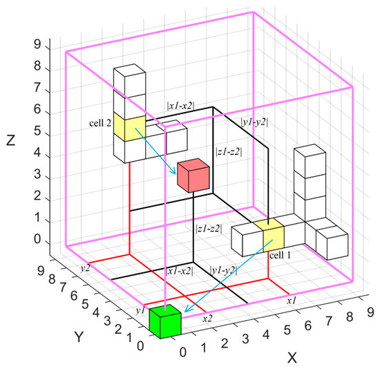
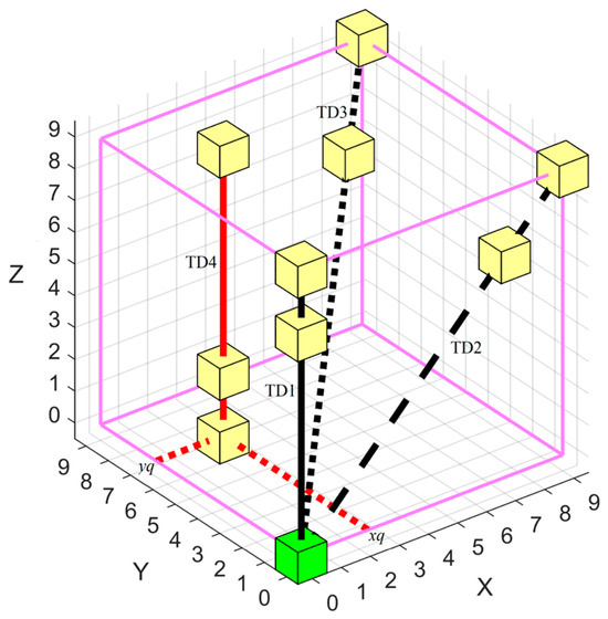
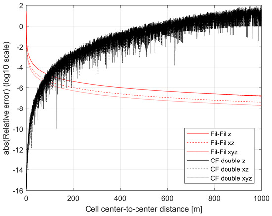
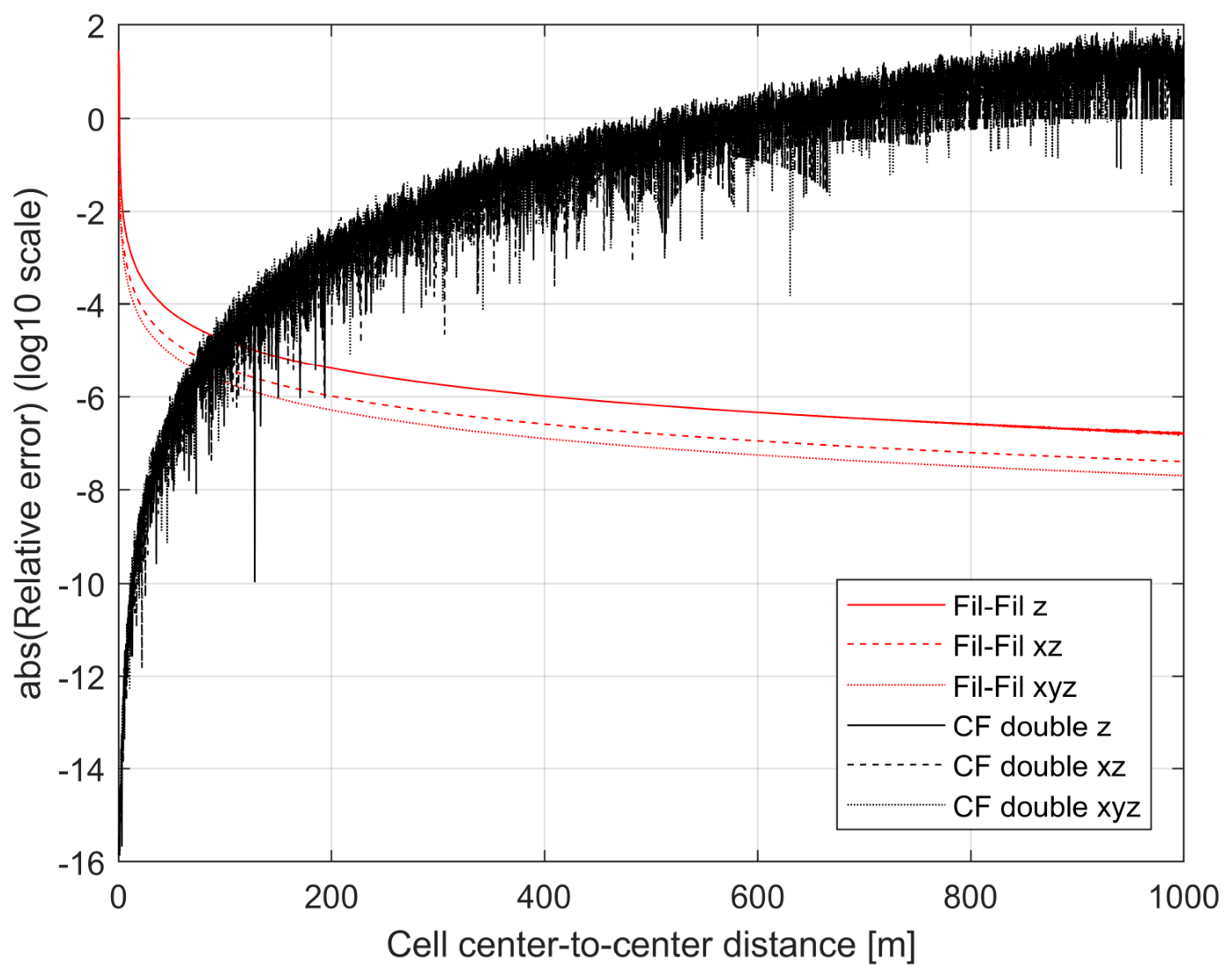
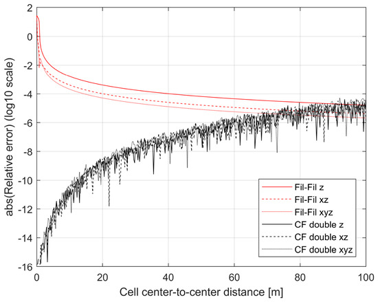
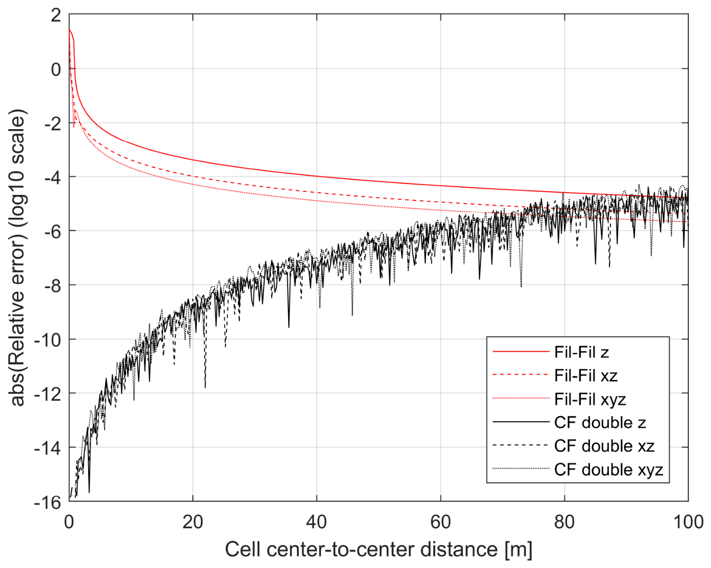
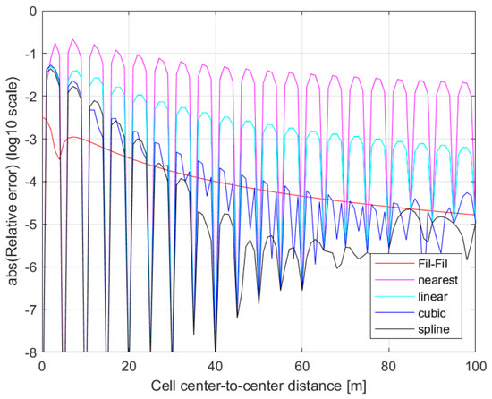
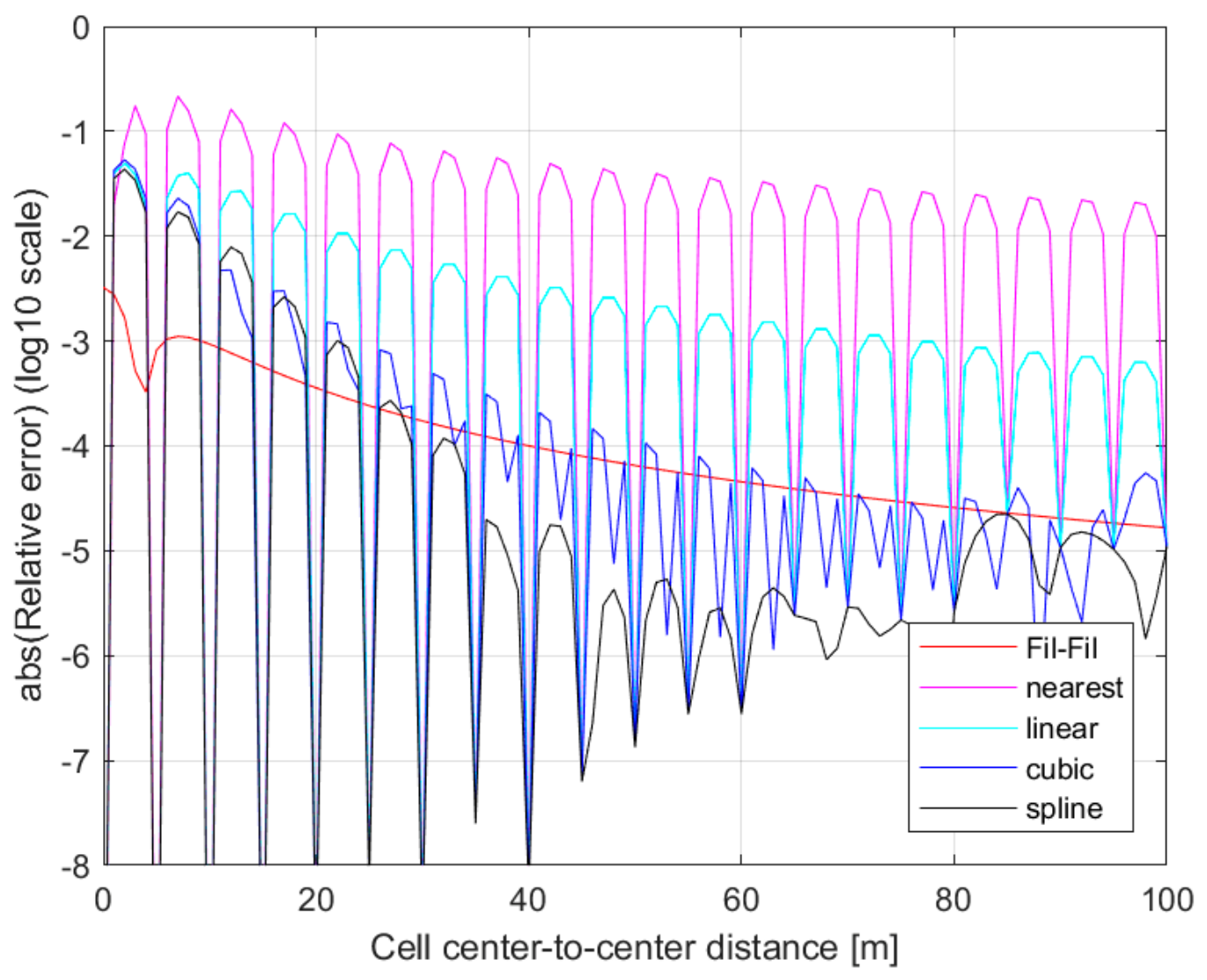
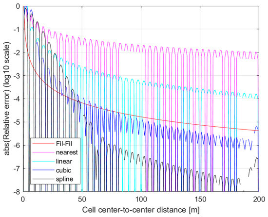
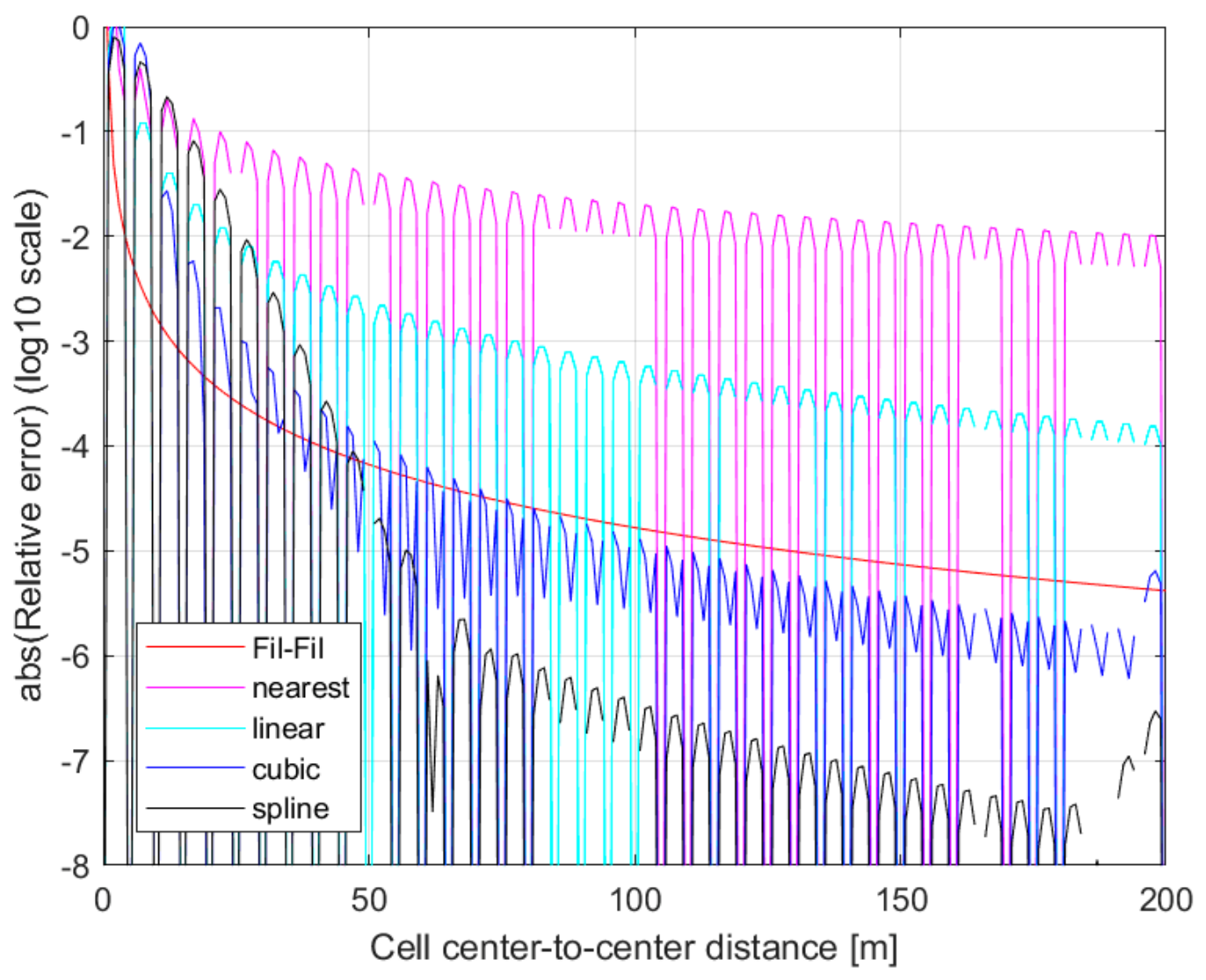
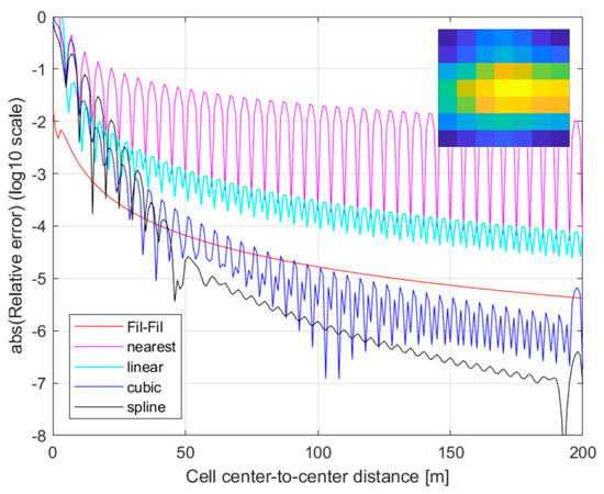
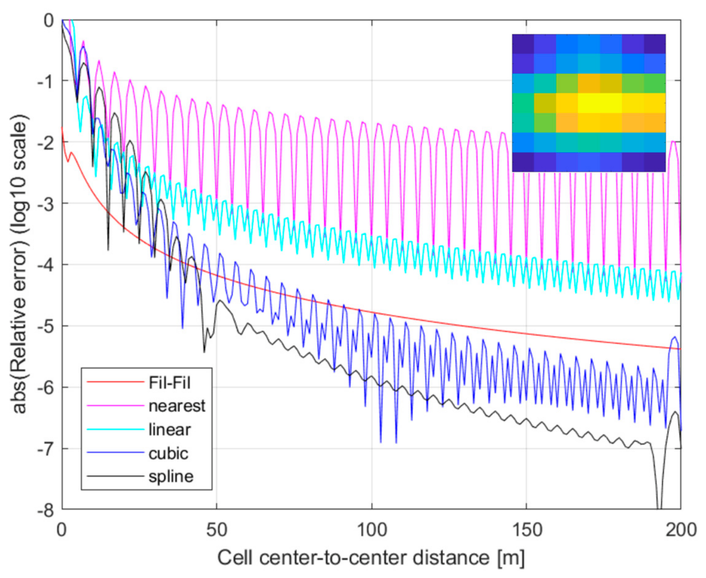
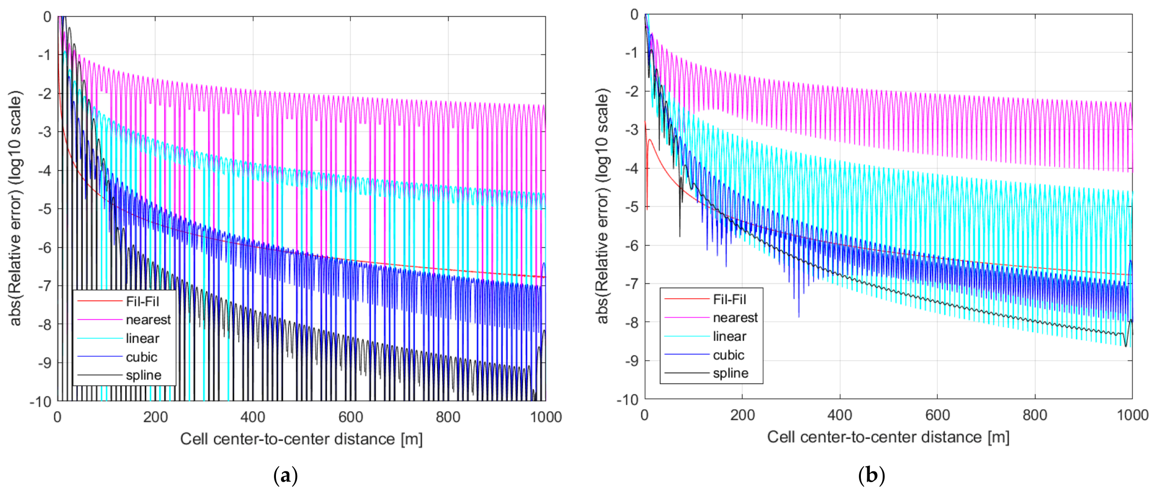
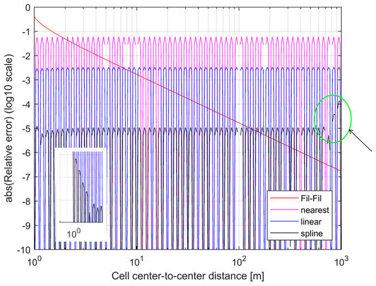
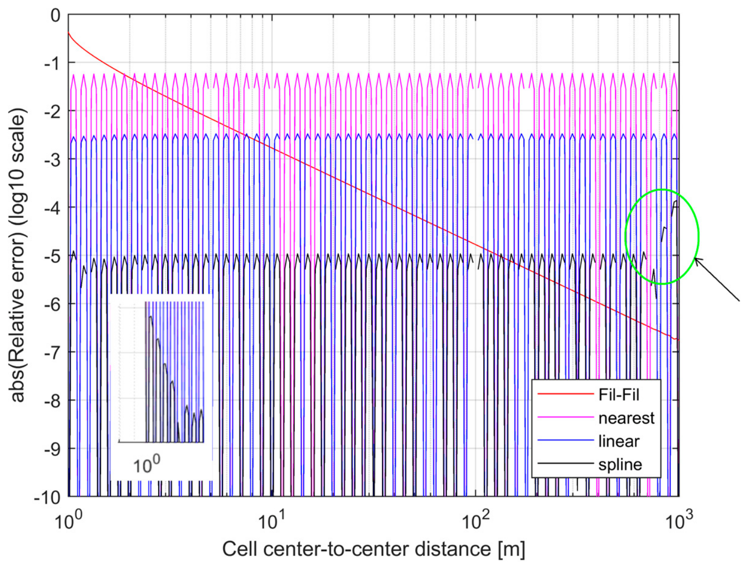
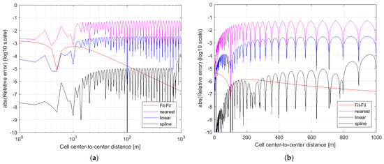
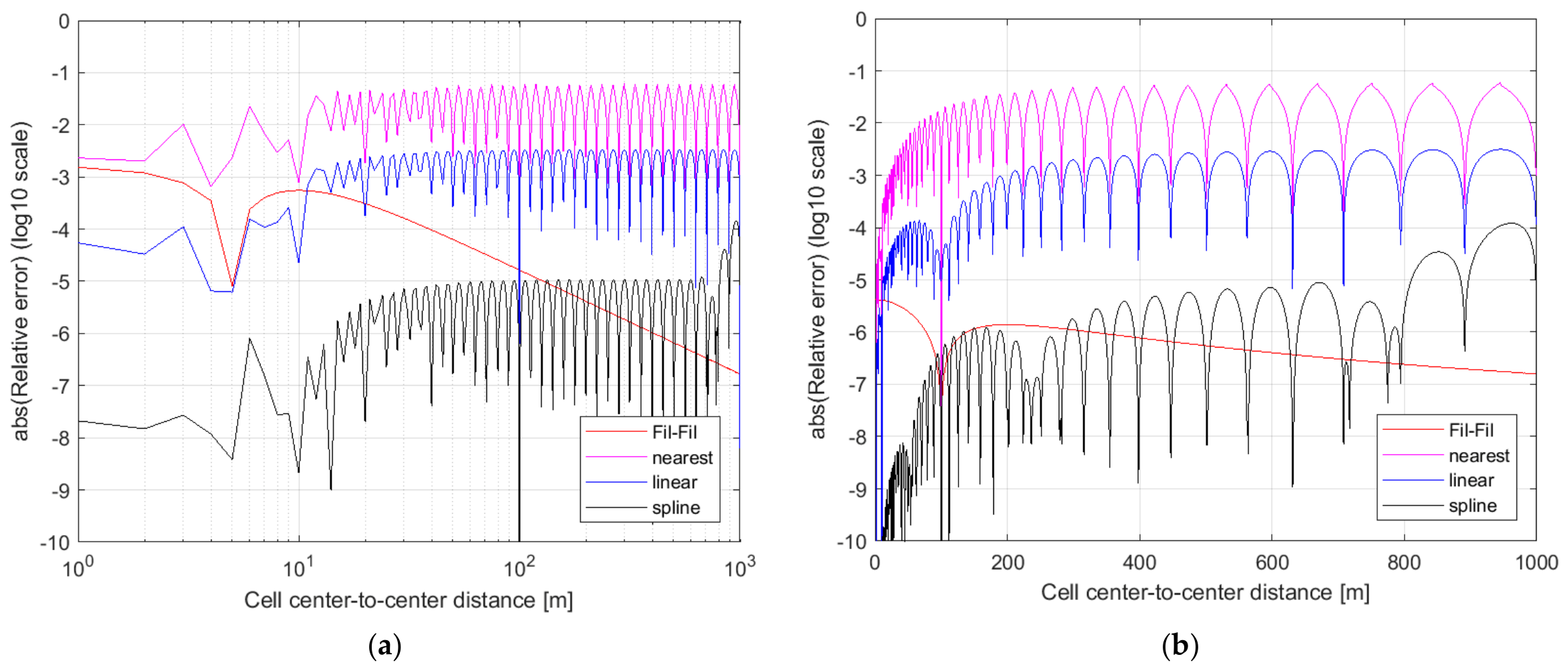
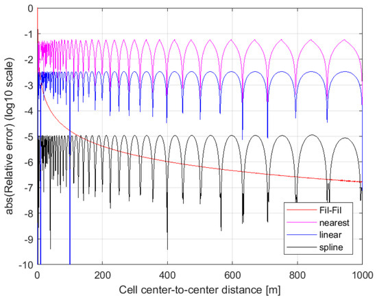
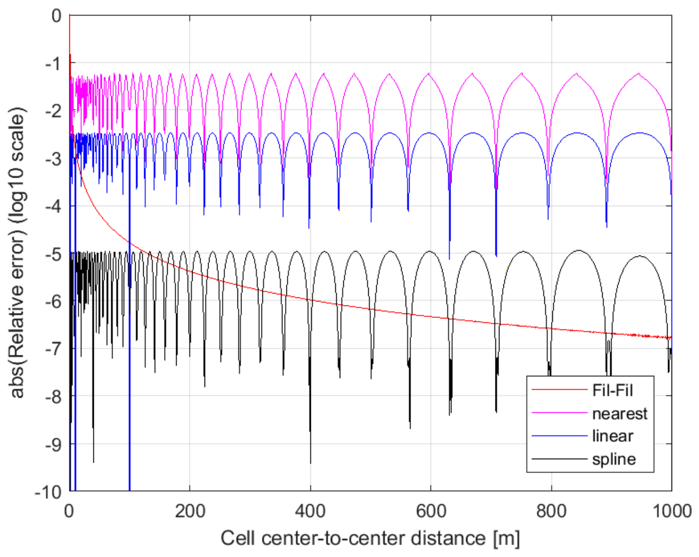

Disclaimer/Publisher’s Note: The statements, opinions and data contained in all publications are solely those of the individual author(s) and contributor(s) and not of MDPI and/or the editor(s). MDPI and/or the editor(s) disclaim responsibility for any injury to people or property resulting from any ideas, methods, instructions or products referred to in the content. |
© 2026 by the authors. Licensee MDPI, Basel, Switzerland. This article is an open access article distributed under the terms and conditions of the Creative Commons Attribution (CC BY) license.