Bayesian Recalibration of Geospatial Liquefaction Model with Regional Data Updating: A Case Study of the 2008 Wenchuan Earthquake

Abstract

Based on the global geospatial liquefaction model, this study adopts updated datasets of 30 m depth-averaged shear wave velocity ($V_{S30}$) and groundwater table depth ($wtd$) for the 2008 Wenchuan earthquake. Two models are then established: the local geospatial liquefaction model (LGLM), based solely on regional data, and the Bayesian-updated geospatial liquefaction model (BGLM), using Bayesian recalibration with global prior information and regional updated data. Model performance is evaluated using stratified five-fold cross-validation and spatial blocked cross-validation. The results show that integrating regional recalibration into the Bayesian framework effectively balances global prior information and regional data characteristics, reduces the global model’s systematic biases in regional applications, and provides accurate, stable, and regionally adaptable predictions within the study area. The Bayesian framework quantifies predictive uncertainty and characterizes performance variability. The uncertainty information obtained is more comprehensive and informative than the single-point AUC metric. Key variables for liquefaction prediction can be identified through Bayesian posterior distribution analysis. Regional updated data optimizes parameter estimation and enhances the regional consistency and interpretability of parameters for the Wenchuan earthquake case, providing supportive information for local engineering risk analysis and preliminary assessment.

1. Introduction

China has complex landforms and frequent seismic activity, making earthquake liquefaction a significant threat to major infrastructure [1]. Targeted regional seismic risk assessment is essential for mitigating safety risks posed by liquefaction-related disasters.

In the early stages, understanding of seismic liquefaction was mainly based on observations and statistical analyses of liquefaction phenomena at earthquake sites, and relevant factors affecting liquefaction were subsequently summarized, including soil fine-particle content, groundwater level, and seismic intensity [2]. Subsequently, with the deepening understanding of the mechanical mechanism of seismic liquefaction, scholars attempted to conduct quantitative evaluation and gradually formed liquefaction evaluation methods including the Seed–Idriss simplified method [3], static cone penetration test [4], shear wave velocity method [5], energy criterion method [6] and multi-parameter combination method [7], realizing the transformation from single-index to multi-index comprehensive evaluation. However, most of the above methods rely on in situ tests, which are costly and time-consuming, making it difficult to characterize the spatial variability of soil parameters at the regional scales and thus limiting their use for large-scale liquefaction risk assessment. Therefore, integrating traditional methods with geographic information systems (GIS), multi-source data, and advanced numerical analysis has attracted extensive attention. This method can comprehensively integrate terrain, soil properties, climatic conditions, water table depth, and seismic zoning, visualize the results, greatly improve information fusion and risk perception capabilities, and realize rapid post-earthquake liquefaction assessment. Meanwhile, with the continuous collection of historical seismic liquefaction case data and the in-depth research on various sensitivity factors of seismic liquefaction in recent years, the paradigm of liquefaction risk assessment has gradually evolved from “point evaluation” to “spatial continuous evaluation” [8,9]. Zhu et al. (2017) [10] proposed a global geospatial liquefaction model (GGLM) that combines multi-scale geospatial information to predict the probability and extent of liquefaction and has been applied in post-disaster emergency scenarios. Li et al. [11] obtained liquefaction samples in the Tangshan earthquake liquefaction area, established a regional liquefaction evaluation model based on four spatial factors, and provided an effective preliminary screening scheme for data-scarce areas. Combining existing seismic liquefaction research with geospatial information, analyzing the potential relationship between liquefaction and attributes such as slope and sediment environment to establish a mapping relationship, and predicting site liquefaction potential using geospatial characteristics triggered by seismic liquefaction have been shown to be effective by numerous studies [12,13,14,15].

GIS-based liquefaction prediction is convenient for site evaluation, but the resulting probabilistic predictions may deviate from reasonable decision-making in engineering practice. On the other hand, Bayesian updating and Markov Chain Monte Carlo (MCMC) methods have the advantage of integrating information and have been used more in geotechnical engineering over the past few years as an effective way to quantify various uncertainties [16]. For example, Shen et al. [17] updated Vs-based generalized linear models using expanded case histories, supporting data-driven model optimization. Sadik and Khoshnevisan [18] used a hierarchical Bayesian framework combined with MCMC to account for regional differences and data variability, thereby establishing more robust and accurate correlations from in situ test data. Namikawa [19] used a Bayesian approach to assess the statistical uncertainty in determining the corrected SPT-N value from observational data. Choi et al. [20] adopted a point-estimate-based Bayesian method to update the parameters of the local probability density function of the damage ratio under different seismic intensities, using data from low-to-moderate earthquakes. Engler et al. [21] proposed a Bayesian updating method for liquefaction models based on local geotechnical data to compensate for the lack of geological and geotechnical constraint information in the original model. Zhao et al. [22] established a Bayesian framework that combines global prior information with site-specific data, providing a direct reference for regional model calibration. Pirhadi et al. [23] used Bayesian mapping functions and logistic regression with bias-sampling sensitivity analysis to improve the reliability of liquefaction prediction under limited data. Moreover, Durap and Balas [24] proposed a hybrid model integrated with a Bayesian network for multi-hazard risk assessment under complex uncertainties, which follows the same philosophy of combining physical models with Bayesian inference. Durap [25] developed a GIS-based Bayesian network model for coastal hazard identification, demonstrating that the spatial Bayesian framework can provide more comprehensive uncertainty information than traditional deterministic single-point evaluation methods. Baise et al. [26] proposed a Bayesian logistic regression framework to regionalize the GGLM for California using local liquefaction observations. This further supports the rationality of combining geospatial data with Bayesian updating for regional liquefaction prediction. In general, such methods comprehensively account for uncertainty and integrate multi-source data, effectively address spatial autocorrelation in model parameters and complex high-dimensional posterior distributions, and provide auxiliary information for risk analysis in practical engineering applications.

At present, research on geospatial liquefaction models in China remains insufficient, and the characterization of model uncertainty in existing studies is fragmented. Different from the traditional regional updating framework dominated by geospatial data calibration, this study constructs a Bayesian geospatial model with informative prior constraints. The proposed model integrates prior information from global liquefaction models and regional observational characteristics to reduce the systematic bias of global models in localized applications. Taking the Wenchuan earthquake as a case study, this paper explores the feasibility and applicability of regional adaptation for global liquefaction models in the Wenchuan area within a Bayesian framework using regionally recalibrated datasets. Furthermore, unlike conventional point-estimation-based Bayesian geotechnical updating methods, this study uses the MCMC algorithm to quantify uncertainty intervals for model parameters and predictions. By systematically comparing the predictive performance of the global liquefaction model, regional model calibration, and Bayesian updating model, the key control factors affecting regional liquefaction prediction accuracy are identified, providing a theoretical reference for further model optimization within similar geological contexts.

2. Liquefaction Data and Geospatial Information

2.1. Liquefaction Data

The 2008 $M_{\mathrm{w}}$ 7.9 Wenchuan earthquake struck the southeastern Qinghai–Tibet Plateau and the upper Minjiang River, an area with complex mountainous terrain, uneven north–south rainfall, and distinct east–west geomorphic differentiation, triggering numerous geological disasters [27].

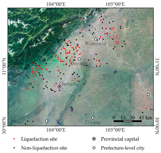
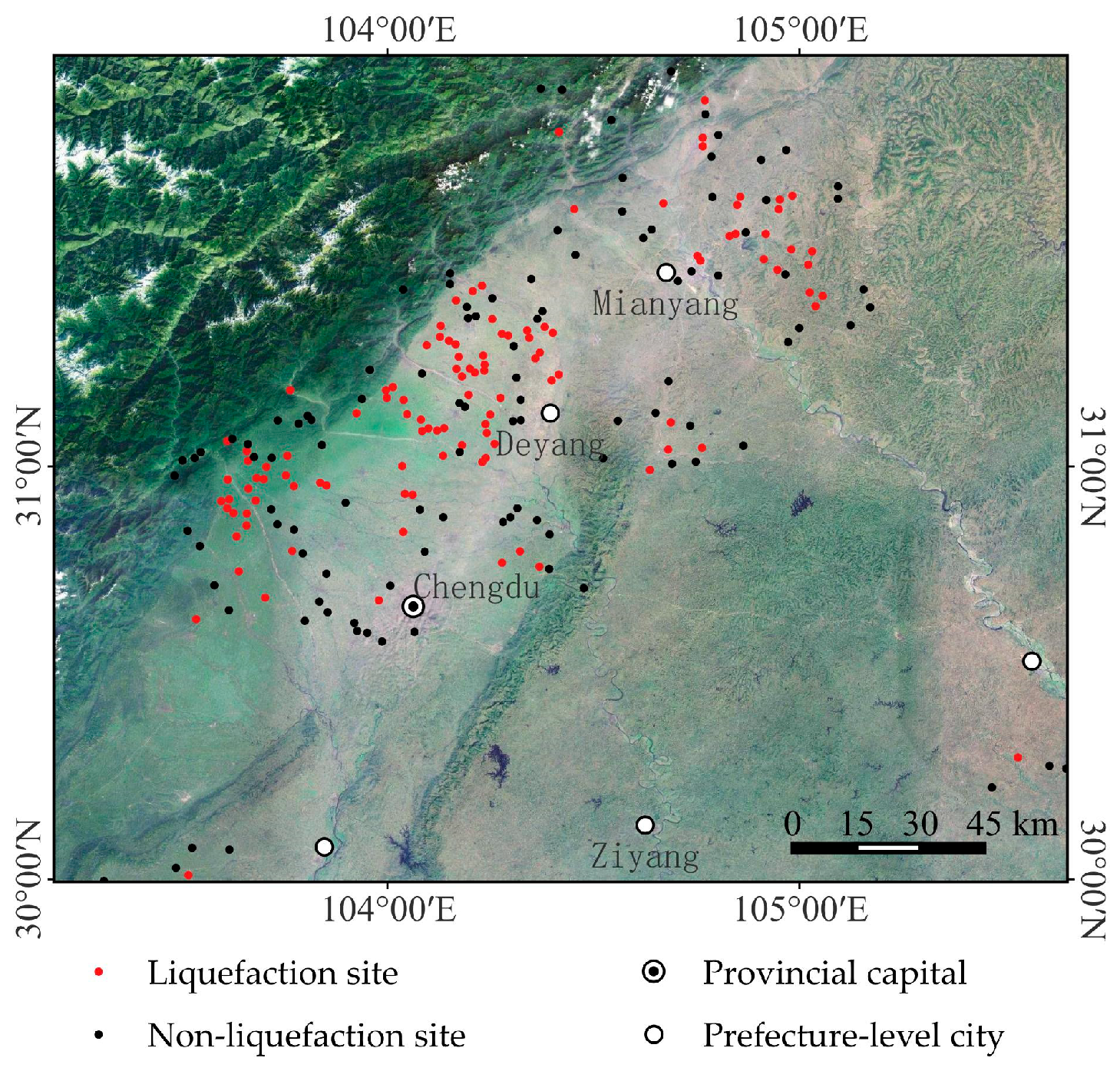
To systematically conduct seismic liquefaction research, this study first selects 116 liquefaction observation points from the Wenchuan earthquake compiled by Zhu et al. (2016) [28] and constructs a liquefaction dataset in QGIS. Next, non-liquefaction points are selected according to the sampling strategy of Zhu et al. (2017) [10] (sampling within a 1–15 km radius of liquefaction points) to build a balanced dataset. This process results in a liquefaction dataset with 232 points. In accordance with the widely recognized 10-rule for regression analysis, this sample size is sufficient. The sample point distribution is shown in Figure 1.

Figure 1. Liquefaction sites in the 2008 Wenchuan earthquake.

2.2. Geospatial Information and Analysis

The geospatial variables used in this study are selected to reflect the main factors related to liquefaction, including seismic loading, soil stiffness and density, and soil saturation. The geospatial information and its respective sources are listed below.

Peak ground velocity (PGV) is the maximum velocity of seismic waves passing through the ground surface and is an important parameter for predicting potential seismic damage. This data can be obtained from the ShakeMap platform developed by the United States Geological Survey (USGS).

Shear wave velocity serves as a fundamental parameter for assessing the liquefaction resistance of rock and soil. Its use for characterizing liquefaction resistance is widely supported by previous studies [5,29,30]. $V_{S30}$ is the depth-weighted harmonic average of shear wave velocity in the upper 30 m, showing the speed of seismic waves through shallow soils. Shallow loose strata, often liquefiable and with low shear wave velocity, usually fall within 30 m depth and lower the $V_{S30}$ value. This connection allows $V_{S30}$ to reflect where shallow, loose deposits are found regionally. Reference [28] shows that most liquefied sites have low $V_{S30}$, while non-liquefied sites have high $V_{S30}$, indicating that $V_{S30}$ distinguishes between liquefied and non-liquefied cases and is applicable to the model in this study. The USGS has used $V_{S30}$ in liquefaction hazard assessments. $V_{S30}$ data are usually measured using a geological survey, a seismic wave-velocity test, or a high-density electrical method. However, due to data acquisition limitations, geological complexity, and other factors, such data are often difficult to obtain or incomplete. Wald and Allen [31] noted that $V_{S30}$ can be approximated using topographic slope. Accordingly, the GGLM adopts this method to obtain $V_{S30}$ data and applies it to the USGS $V_{S30}$ dataset for seismic liquefaction probability calculation. To further improve data quality, Zhou et al. [32] integrated borehole data from 7939 engineering sites and strong motion stations in Chinese mainland, optimizing the data for China using a topographic slope co-kriging model. Their research shows that these new $V_{S30}$ data are superior to USGS $V_{S30}$ data in geomorphic differentiation, sedimentary environment discrimination, and the rationality of mountain terrain processing.

Hydrological conditions are key media for seismic liquefaction. Annual average precipitation ($precip$), distance to the nearest water body ($dw$) and water table depth ($wtd$) reflect the influence of soil saturation from three dimensions: rainfall infiltration recharge intensity, groundwater dynamic condition and pore water pressure state. This study uses monthly average precipitation data from 1970 to 2000 (climate baseline period) of the WorldClim global climate dataset to obtain $precip$ data through QGIS spatial analysis. $dw$ is mainly defined as the minimum of distance to the nearest ocean ($dc$) and distance to the nearest river ($dr$), reflecting soil water infiltration and sedimentary states. Among them, $dr$ and $dc$ data can be obtained from HydroSHEDS and NASA OPG datasets, respectively. For $wtd$ data, estimation is based on the early model of Fan et al. (2013) [33], combined with the research of Fan and Miguez-Macho [33], who optimized equilibrium groundwater table models by integrating vertical soil water balance, groundwater recharge–discharge, water table fluctuations, and adaptive root water uptake depth. This enabled interactions among soil water, surface water, groundwater, and vegetation water use, effectively resolving the overestimation of water tables in early models.

To summarize the date update process, this study selects two main parameter data, $V_{S30}$ and $wtd$, for updating, while other geospatial parameter data remain unchanged. None of the geospatial data were derived from liquefaction observations, nor do they influence the validity of model predictions. Summary statistics for the collected data are provided in Table 1. The optimized geospatial data above are applied to all models in this study.

Table 1. Numerical characteristics of seismic liquefaction data.

Parameters	Unit	Mean	Standard Deviation	Median
$\mathrm{l}\mathrm{n}\left(\mathrm{P}\mathrm{G}\mathrm{V}\right)$	cm/s	3.044	0.632	3.024
$\mathrm{l}\mathrm{n}\left(V_{S30}\right)$	m/s	5.773	0.163	5.738
$precip$	mm	996.4	138.1	948.0
$dw$	km	2.380	1.851	1.856
$wtd$	m	11.742	18.308	2.610

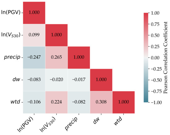
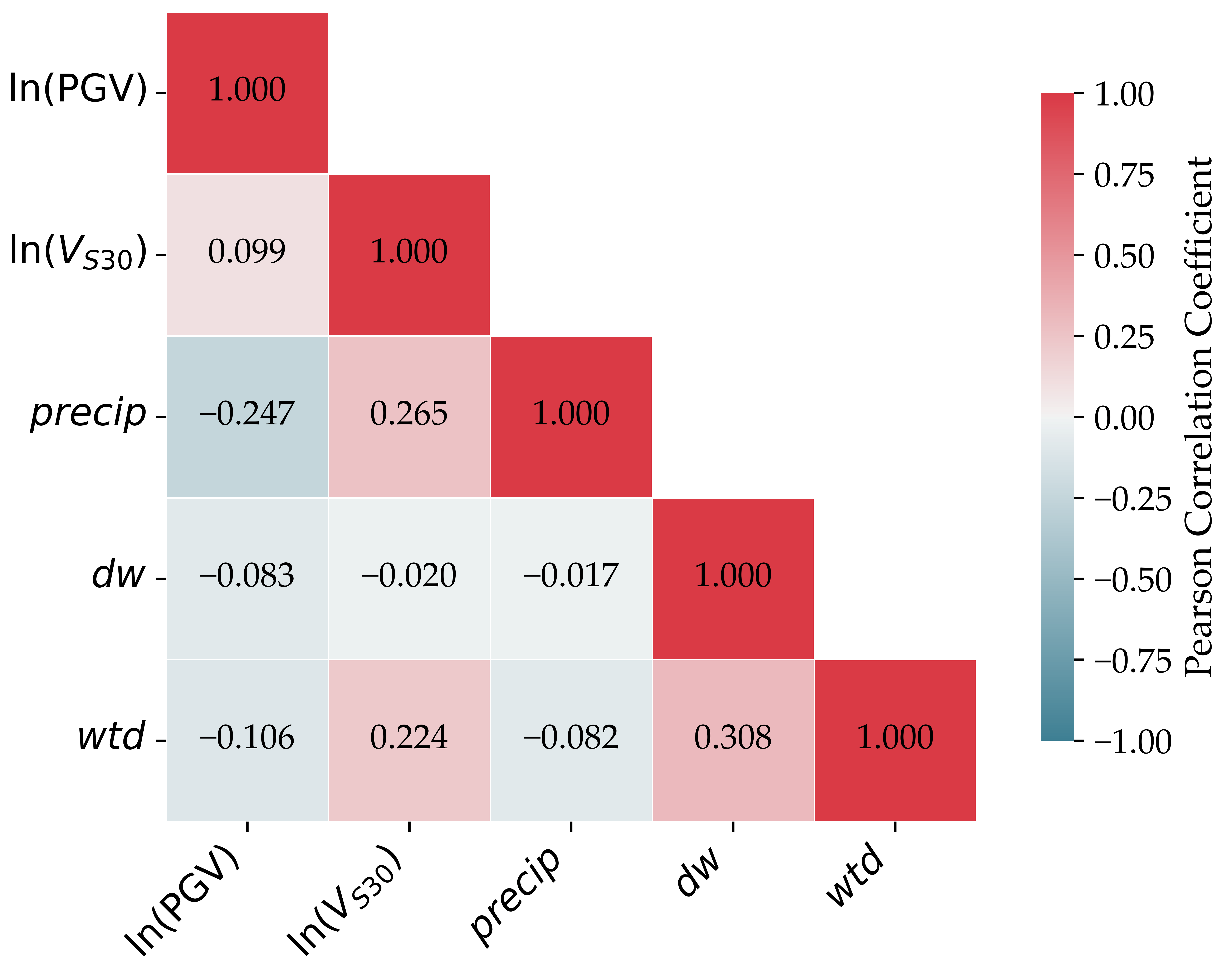
Before model construction, Pearson correlation analysis was conducted for all geospatial parameters, as shown in Figure 2. The results indicate that all absolute correlation coefficients are less than 0.31, suggesting an extremely weak linear relationship among variables. All parameters were standardized before multicollinearity diagnosis. As listed in Table 2, the variance inflation factor (VIF) values range from 1.12 to 1.24, all of which are far below 5. No significant multicollinearity is observed, so all variables can be safely and reliably introduced into the regression models.

Figure 2. Pearson correlation matrix of geospatial parameters.

Table 2. Variance Inflation Factor (VIF) values for multicollinearity diagnosis of geospatial parameters.

	$\mathbf{l}\mathbf{n}\left(\mathbf{P}\mathbf{G}\mathbf{V}\right)$	$\mathbf{l}\mathbf{n}\left({\mathit{V}}_{\mathit{S}30}\right)$	$\mathit{P}\mathit{r}\mathit{e}\mathit{c}\mathit{i}\mathit{p}$	$\mathit{d}\mathit{w}$	$\mathit{w}\mathit{t}\mathit{d}$
VIF	1.14	1.22	1.22	1.12	1.24

2.3. Limitations and Rationale of $V_{S30}$

$V_{S30}$ is widely used as a site-classification index in seismic codes and ground-motion response analyses [34,35]. However, its physical association with liquefaction triggering remains indirect and largely phenomenological.

From a mechanistic perspective, shear wave velocity is governed by the small-strain shear stiffness of soils, which is closely related to soil density, effective confining pressure, soil type, gradation, consolidation state, and stress history. $V_{S30}$ represents the overall stiffness of the upper 30 m of soil deposits and may indirectly reflect the presence of shallow loose sediments, as low-velocity liquefiable soils at depths up to 30 m tend to reduce the bulk $V_{S30}$ value. In this way, $V_{S30}$ serves as a general, macroscopic indicator of regional liquefaction susceptibility.

Nevertheless, as a depth-averaged index, $V_{S30}$ has certain limitations for liquefaction evaluation. It is less effective at capturing shallow liquefiable layers, reflecting local stratigraphic variability, and identifying thin weak deposits that control liquefaction behavior. Owing to its 30 m depth averaging, it cannot reliably resolve critical liquefiable layers within the upper 0–10 m, which often dominate liquefaction triggering. The averaging effect tends to smooth local stratigraphic variations and may not fully represent true soil heterogeneity. Additionally, signals from thin, weak layers that control site liquefaction potential can be masked by the overall average, making them difficult to identify reliably [36].

In this study, $V_{S30}$ is still adopted because it provides spatially continuous and globally accessible data, supporting rapid regional liquefaction prediction in areas where borehole or geotechnical data are limited. Studies have confirmed that $V_{S30}$ exhibits a reasonable correlation with liquefaction probability [10,37]. Meanwhile, Kongar et al. [38] verified the performance of $V_{S30}$ using field observations from the Darfield and Christchurch earthquakes in New Zealand, supporting its suitability for regional rapid liquefaction assessment. Furthermore, combining $V_{S30}$ with other geospatial parameters in the model may help alleviate some of its limitations. Therefore, $V_{S30}$ can be used as one of the practical macroscopic proxy indicators for regional liquefaction risk assessment.

3. Geospatial Liquefaction Models

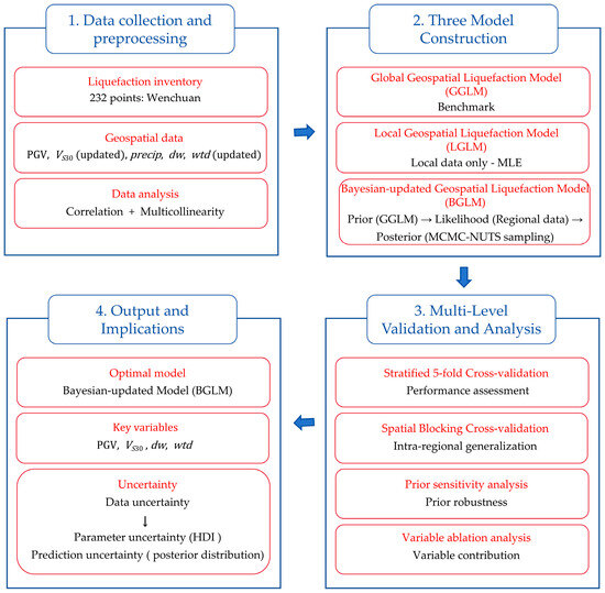
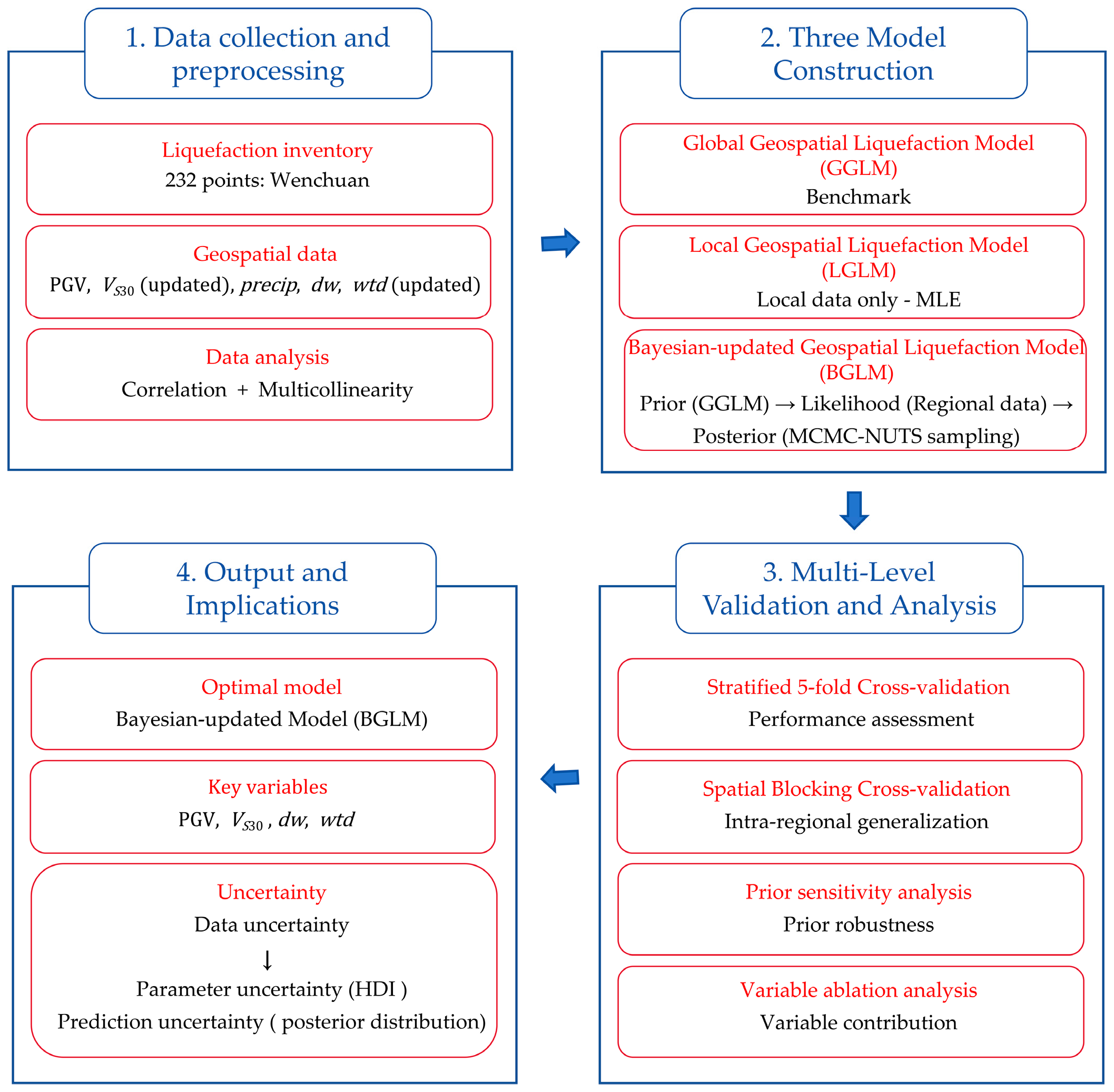
After data collection and preprocessing, in this section, three geospatial liquefaction models are constructed based on the Wenchuan earthquake liquefaction database: the Global Geospatial Liquefaction Model (GGLM) as the benchmark, the Local Geospatial Liquefaction Model (LGLM) fitted solely on regional data via maximum likelihood estimation, and the Bayesian-updated Geospatial Liquefaction Model (BGLM), which leverages informative priors from the GGLM and NUTS-based MCMC sampling to achieve stable parameter calibration and uncertainty quantification. Geospatial indicators, including peak ground velocity ($\mathrm{P}\mathrm{G}\mathrm{V}$), updated 30 m depth-averaged shear wave velocity (${\mathrm{V}}_{\mathrm{S}30}$), annual mean precipitation ($precip$), distance to the nearest water body ($\mathrm{d}\mathrm{w}$), and updated groundwater table depth ($wtd$), are selected to effectively characterize site-specific liquefaction conditions. Prior to modeling, correlation and multicollinearity analyses were already completed in the preceding section to eliminate collinearity issues among variables. The liquefaction assessment framework is implemented using QGIS for spatial data processing, Python 3.10 for statistical modeling, and MCMC sampling for Bayesian inference. Model performance, generalization ability, robustness, and variable contribution will be systematically evaluated in the following section through a multilevel validation scheme, including stratified cross-validation, spatial blocking cross-validation, prior sensitivity analysis, and variable ablation analysis. The overall research workflow, including multi-level validation and uncertainty propagation, is presented in Figure 3.

Figure 3. Technical workflow of this study.

3.1. Geospatial Liquefaction Model Based on Regional Data Updating

Zhu et al. (2015) [39] developed a geospatial model for liquefaction assessment based on logistic regression. Based on liquefaction data from the 1995 Hyogo-ken Nanbu earthquake in Japan and the 2010–2011 Christchurch earthquake in New Zealand, peak ground acceleration ($\mathrm{P}\mathrm{G}\mathrm{A}$), $V_{S30}$ derived from topographic slope, normalized distance to coast ($\mathrm{N}\mathrm{D}$), and compound topographic index ($\mathrm{C}\mathrm{T}\mathrm{I}$) were selected as proxy variables to quantify seismic action, soil properties and site water conditions, respectively, establishing a mapped relationship between geospatial information and liquefaction probability. However, this model is only applicable to coastal environments, is difficult to apply in non-coastal areas because of hydrological differences, and has limited global applicability due to its small sample size. Zhu et al. (2017) [10] systematically optimized the liquefaction model and constructed GGLM: on the one hand, the sample size was expanded to 27 earthquakes covering different magnitudes, geological backgrounds and climate zones, and non-liquefaction samples were obtained through sampling strategies; on the other hand, proxy variables were re-screened, and it was found that $\mathrm{P}\mathrm{G}\mathrm{V}$ better reflects the triggering effect of long-period vibration on liquefaction than $\mathrm{P}\mathrm{G}\mathrm{A}$. Parameters such as $precip$, $dw$ and $wtd$ were added to characterize hydrological conditions in non-coastal areas, and a five-variable regression expression for non-coastal areas was proposed (Equations (1) and (2)):

$$P(X)={\displaystyle \frac{1}{1+e^{-X}}}$$

(1)

$$X=8.801+0.334\ln (\mathrm{P}\mathrm{G}\mathrm{V})-1.918\ln (V_{S30})+5.408\times 10^{-4}precip-0.2054dw-0.0333wtd$$

(2)

where $P$ is the probability of liquefaction occurrence, and $X$ is the linear combination of geospatial parameters. Meanwhile, according to the liquefaction limit observation of $\mathrm{P}\mathrm{G}\mathrm{V}$ and $V_{S30}$, the variable threshold range for liquefaction occurrence is derived: $\mathrm{P}\mathrm{G}\mathrm{V}>3\mathrm{c}\mathrm{m}/\mathrm{s}$ or $V_{S30}<620\mathrm{m}/\mathrm{s}$. Rashidian et al. [40] added liquefaction conditions of $\mathrm{P}\mathrm{G}\mathrm{A}>0.1\mathrm{g}$ and $precip<1700\mathrm{m}\mathrm{m}$.

By leveraging sample expansion, variable optimization, and strengthened physical constraints, the GGLM establishes an evaluation framework with accessible data and reliable predictions, serving as a practical tool for post-earthquake rapid response and large-scale risk screening. Thus, GGLM is utilized as the benchmark for model comparison in this research. Based on the GGLM framework, this study abandons its original parameter and data system and constructs a local geospatial liquefaction model (LGLM) using locally refined data for the study area. LGLM uses full liquefaction data, completes parameter learning and model fitting through logistic regression maximum likelihood estimation based on updated $V_{S30}$ and $wtd$ data, ensures model convergence, and realizes GGLM reconstruction based on site-specific regional data; then, model performance is approximately evaluated using each fold test set divided by cross-validation in this study to obtain corresponding results.

3.2. Bayesian-Updated Model Integrating Prior Information and Regional Recalibration

The essence of Bayesian inference is to dynamically revise the probabilistic beliefs about unknown parameters based on observed data, and its core framework is defined by the Bayesian formula. Let geospatial parameters be $\theta$ and initial observation data be $D$, then the posterior distribution of parameter $\theta$ satisfies (Equation (3)):

$$P(\theta \mid D)\propto P\left(\theta \right)\cdot P(D\mid \theta )$$

(3)

where $P\left(\theta \right)$ is the prior distribution of geospatial parameters, $P\left(D|\theta \right)$ is the likelihood function of seismic liquefaction observation data, and $P\left(\theta |D\right)$ is the posterior distribution integrating prior information and data updating information.

In geospatial liquefaction models, high-dimensional integrals involved in Bayesian inference of multi-dimensional parameters are usually difficult to evaluate analytically, and traditional numerical integration is highly inefficient. MCMC methods can effectively estimate posterior distributions by virtue of their sampling advantages for complex distributions. The core is to construct a Markov chain that is consistent with the state and parameter spaces. After the Markov chain converges, the initial transition samples are removed, and the remaining valid samples can be approximated as independent and identically distributed samples of the target posterior distribution. The posterior characteristics of geospatial parameters are estimated through sample statistics. Among various MCMC algorithms, the No-U-Turn sampler (NUTS) is widely used in high-dimensional models, as it can adaptively adjust the step size and mass matrix, reduce sample autocorrelation, and improve sampling efficiency. Durap et al. [41] adopted Bayesian theory combined with Monte Carlo simulation to develop a comprehensive risk assessment system that integrates prior experience and site observation data for liquefaction-related disaster evaluation and provides conceptual support for the application of MCMC posterior estimation in this study.

Traditional logistic regression often leads to unstable parameter estimation due to insufficient data volume in small-sample liquefaction prediction scenarios. Therefore, this study introduces Bayesian updating combined with MCMC sampling to suppress overfitting and naturally quantify predictive uncertainty. Based on this framework, a Bayesian-updated geospatial liquefaction model (BGLM) is constructed to perform Bayesian recalibration by integrating global prior information from the GGLM and regional updated data. This model belongs to Bayesian logistic regression with informative priors, rather than a hierarchical Bayesian spatial model that incorporates latent spatial processes (e.g., Gaussian process, CAR/ICAR). Its primary purpose is parameter calibration and uncertainty quantification through Bayesian updating.

In the prior parameter setting of BGLM, because there is no domain consensus as a prior basis for geospatial parameters in liquefaction prediction, the direct use of non-informative priors can easily lead to parameter oscillation in small samples. Such unstable fluctuation could affect model convergence and estimation credibility. Therefore, this study adopts an informative prior strategy to balance parameter stability in limited-data settings, i.e., using the GGLM parameter point estimates as the prior mean. These parameters are calibrated against global multi-area liquefaction records and reflect general inherent laws of liquefaction occurrence, which makes them qualified as reliable initial constraints for regional modeling. Constraining the parameter space can effectively avoid model overfitting when the data volume is insufficient. For prior scale adjustment, the reasonable fluctuation range of parameters is preliminarily defined based on the uncertainty analysis results from Zhan et al. [42]. This study adopts the conventional setting idea of Bayesian regression models to keep prior scales consistent with parameter magnitudes [43]. This differentiated scale adjustment follows weakly informative prior design principles. We moderately relax the prior range for parameters with updated local data to reduce prior restraint and let field observations dominate parameter revision. Non-updated parameters keep their original narrow scales to maintain the fundamental characteristics of the global reference model [26]. Multiple scale schemes are tested and compared, and the final prior scales are determined as 8, 0.06, 3, 0.0003, 0.04, and 0.1 after balancing constraint intensity and regional data adaptability.

In the MCMC sampling step, the NUTS algorithm is used. After warm-up to remove invalid samples and pass validity tests, the parameter posterior distribution is obtained, model construction is completed, and model evaluation results are output. Convergence diagnostics were performed for all MCMC simulations. The potential scale reduction factor (R-hat) for all parameters was less than 1.01, and the effective sample size (ESS) for each posterior distribution exceeded 1000. These results confirm that all Markov chains converged adequately and that the posterior estimates are reliable.

Meanwhile, to verify the rationality and stability of the prior settings, a prior sensitivity analysis was conducted by setting the prior scales to 0.5 times, 1.0 times (baseline), and 2.0 times the original values. The posterior means and standard deviations under different prior strengths were compared, as summarized in Table 3.

Table 3. Posterior statistics under different prior scales.

Parameters	×0.5		×1.0		×2.0		${\mathit{\mu }}^{\mathbf{*}}$ Variation Rate (%)	${\mathit{\sigma }}^{\mathbf{*}}$ Ratio	Robustness
	${\mathit{\mu }}^{\mathbf{*}}$	${\mathit{\sigma }}^{\mathbf{*}}$	${\mathit{\mu }}^{\mathbf{*}}$	${\mathit{\sigma }}^{\mathbf{*}}$	${\mathit{\mu }}^{\mathbf{*}}$	${\mathit{\sigma }}^{\mathbf{*}}$
intercept	−0.140	0.178	−0.155	0.183	−0.160	0.185	3.56	1.012	Yes
$\mathrm{l}\mathrm{n}\left(\mathrm{P}\mathrm{G}\mathrm{V}\right)$	0.212	0.019	0.216	0.037	0.231	0.071	6.92	1.898	Yes
$\mathrm{l}\mathrm{n}\left(V_{S30}\right)$	−0.554	0.161	−0.651	0.198	−0.689	0.215	5.86	1.087	Yes
$precip$	0.072	0.022	0.067	0.041	0.052	0.075	22.70	1.843	No
$dw$	−0.374	0.037	−0.365	0.072	−0.342	0.129	6.43	1.795	Yes
$wtd$	−0.867	0.246	−0.895	0.260	−0.910	0.265	1.77	1.023	Yes

Note: ×0.5, ×1.0, and ×2.0 represent halved, baseline, and doubled prior scales, respectively. ${\mu }^{*}$ denotes standardized mean, and ${\sigma }^{*}$ denotes standardized standard deviation. Parameters with posterior mean variation rate less than 10% are regarded as robust. All statistical results are obtained based on standardized variables.

The results show that the posterior estimates of all parameters were generally consistent across different prior specifications. When the prior scale was doubled, the posterior means of most parameters varied by less than 7%, and the changes in posterior standard deviations were limited. Only the $precip$ parameter showed a relatively large variation rate of 22.70%, which was related to its low contribution and high uncertainty in the model. Overall, the posterior results were robust to prior settings, demonstrating that the prior configuration in this study is reasonable and does not bias the posterior.

4. Results and Analysis

4.1. Stratified Five-Fold Cross-Validation

This section first estimates model parameters and evaluates significance using a stratified five-fold cross-validation strategy. On this basis, the variation laws of model parameters before and after Bayesian updating are clarified, and the influence mechanisms of global prior constraints and regional measured data on parameter calibration are revealed, thereby verifying the rationality of the proposed prior-setting scheme and model-optimization idea. Subsequent sections will further compare and discuss the prediction performance, uncertainty quantification effect and practical application value of different models, and relevant spatial blocking cross-validation or leave-one-event-out validation will be supplemented in follow-up research to further verify regional transferability and true generalization performance of geospatial models.

4.1.1. Parameter Estimation

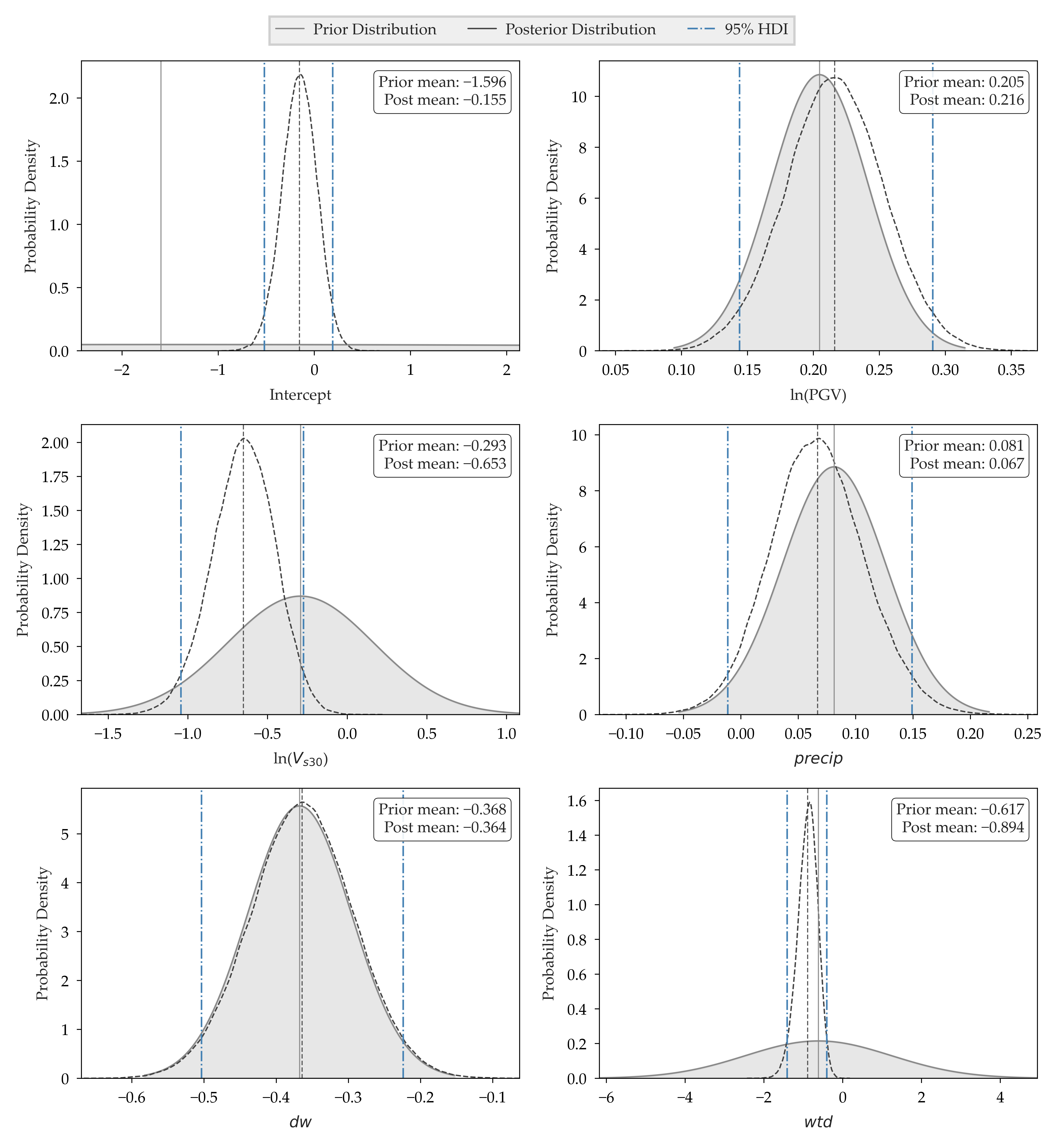
In this study, the parameters of the established Bayesian-updated model are determined using the MCMC method, and the results are presented in Table 4 and Table 5 and Figure 4.

Table 4. Summary of parameter estimates for all models.

Model	Intercept	$\mathbf{l}\mathbf{n}\left(\mathbf{P}\mathbf{G}\mathbf{V}\right)$	$\mathbf{l}\mathbf{n}\left({\mathit{V}}_{\mathit{S}30}\right)$	$\mathit{P}\mathit{r}\mathit{e}\mathit{c}\mathit{i}\mathit{p}$	$\mathit{d}\mathit{w}$	$\mathit{w}\mathit{t}\mathit{d}$
GGLM	8.801	0.334	−1.918	5.408 × 10−4	−0.2054	−0.0333
LGLM	23.067	0.527	−4.120	−1.050 × 10−4	−0.1545	−0.0466
	(0.417) #	(0.048) #	(0.000) #	(0.933) #	(0.083) #	(0.000) #
BGLM	22.511	0.343	−4.011	4.915 × 10−4	−0.1975	−0.0490
	(9.312, 35.567) *	(0.225, 0.458) *	(−6.350, −1.789) *	(−0.00008, 0.00107) *	(−0.2742, −0.1221) *	(−0.0775, −0.0214) *

Note: ^# Values in parentheses are p-values of parameter coefficients for LGLM. * Values in brackets are 95% highest posterior density intervals of parameter coefficients for BGLM. Values in this table are the destandardized parameter coefficients after inverse transformation from standardized regression.

Table 5. Posterior summary of parameters and effect evaluation for BGLM.

		Intercept	$\mathbf{l}\mathbf{n}\left(\mathbf{P}\mathbf{G}\mathbf{V}\right)$	$\mathbf{l}\mathbf{n}\left({\mathit{V}}_{\mathit{S}30}\right)$	$\mathit{P}\mathit{r}\mathit{e}\mathit{c}\mathit{i}\mathit{p}$	$\mathit{d}\mathit{w}$	$\mathit{w}\mathit{t}\mathit{d}$
${\mu }^{*}$		−0.155	0.216	−0.653	0.067	−0.364	−0.894
${\sigma }^{*}$		0.182	0.037	0.197	0.041	0.071	0.258
$\overline{p}$	$P_r\left(+\right)$	0.197	1.000	0.000	0.953	0.000	0.000
	$C$	$\mathrm{N}\mathrm{S}$	$\mathrm{S}\mathrm{i}\mathrm{g}$	$\mathrm{S}\mathrm{i}\mathrm{g}$	$\mathrm{N}\mathrm{S}$	$\mathrm{S}\mathrm{i}\mathrm{g}$	$\mathrm{S}\mathrm{i}\mathrm{g}$

Note: ${\mu }^{*}$: standardized mean; ${\sigma }^{*}$: standardized standard deviation; $\overline{p}$: average significance; $P_r\left(+\right)$: positive probability; $C$: consistency; $\mathrm{N}\mathrm{S}$: consistently insignificant; $\mathrm{S}\mathrm{i}\mathrm{g}$: consistently significant.

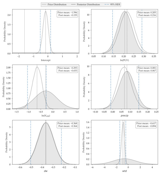
Figure 4. Posterior distributions of standardized BGLM parameters.

In terms of parameter characteristics, Table 4 shows that the coefficients for recalibrated variables in BGLM are close to those in LGLM, whereas those for non-updated variables are consistent with those in GGLM. This objective feature indicates that BGLM adaptively adjusts parameters to fit regional data characteristics while retaining global prior constraints on non-updated variables, thereby effectively integrating global prior knowledge and regional updated information.

The incorporation of local observational data substantially alters the posterior distribution of the model’s parameters. For the $\mathrm{l}\mathrm{n}\left(V_{S30}\right)$ term, the coefficient changes from −1.918 in the GGLM to −4.011 in the BGLM, with the standardized posterior mean decreasing from −0.293 to −0.653. Its 95% highest density interval (HDI) is estimated at [−1.043, −0.275], narrower than the prior distribution and entirely located within the negative significance range. The stable sample standard deviation of 0.163 suggests that this parameter adjustment is only weakly affected by data dispersion, implying that regional data updates effectively constrain posterior parameter variation. Similarly, the standardized posterior mean of the $wtd$ coefficient declines from −0.617 to −0.894, accompanied by obvious shrinkage of its posterior interval. These parameter variations suggest that regional recalibration may strengthen the explanatory power of key variables for liquefaction susceptibility, and the Bayesian updating framework can refine parameter estimation and improve the physical interpretability of model coefficients. Other parameters show relatively minor posterior changes: $\mathrm{l}\mathrm{n}\left(\mathrm{P}\mathrm{G}\mathrm{V}\right)$ exhibits a slightly enhanced positive effect on liquefaction, while $precip$ presents a weakened positive influence. The posterior distribution of the $dw$ parameter is generally consistent with its prior distribution, validating the rationality of the prior-constraint strategy adopted for non-updated parameters in this study.

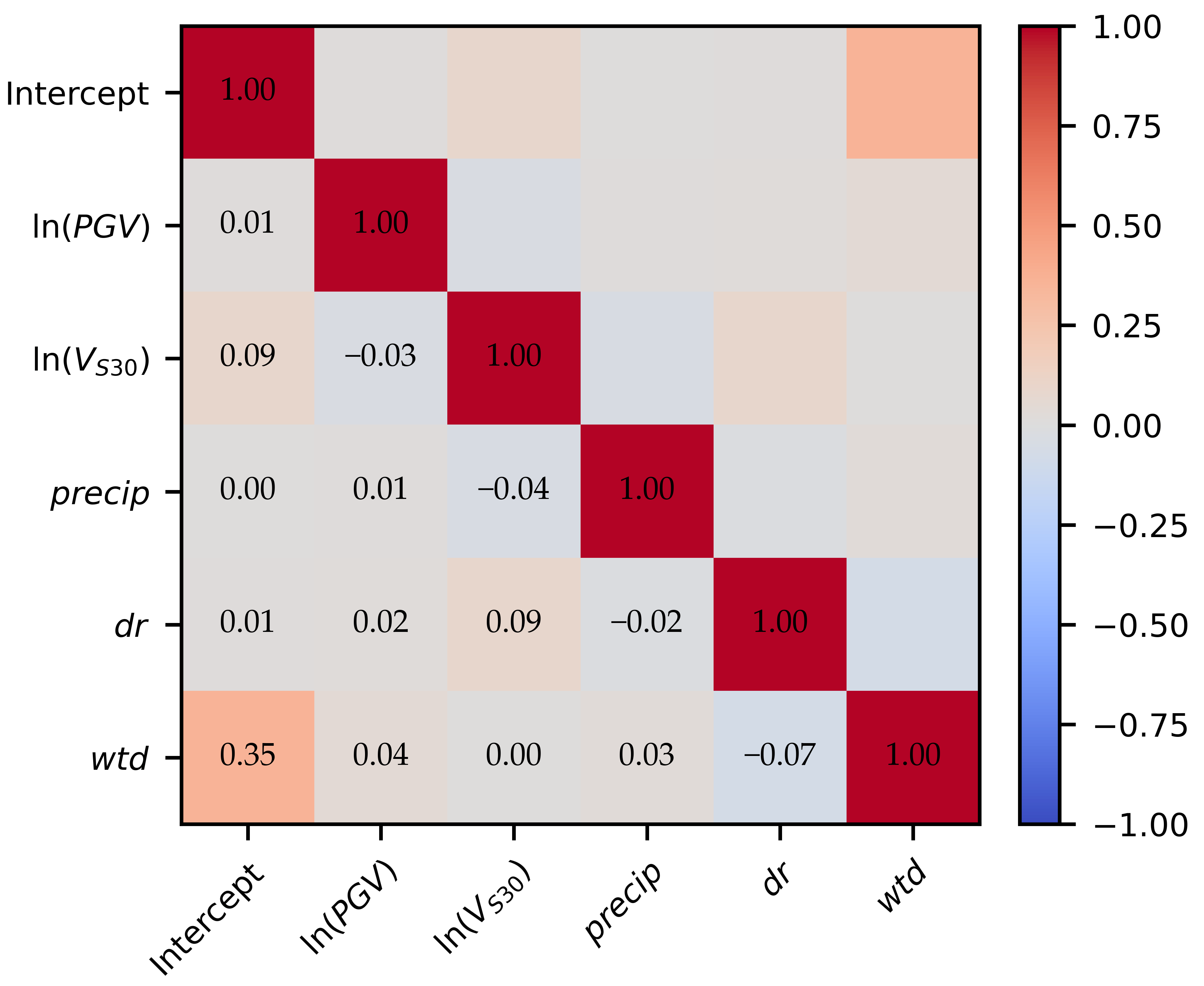
Meanwhile, the 95% HDI of the intercept is wide, indicating weak identifiability. This is mainly due to the loose prior distribution assigned to the intercept term, and the parameter correlation analysis is provided in Appendix A.

4.1.2. Model Parameter Estimation Evaluation

According to the significance test results in Table 4 and Table 5, $\mathrm{l}\mathrm{n}\left(V_{S30}\right)$ and $wtd$ variables show robust statistical significance in both LGLM and BGLM, with convergent posterior distributions in the Bayesian framework, confirming their dominant contributions to liquefaction prediction. In the LGLM, $\mathrm{l}\mathrm{n}\left(\mathrm{P}\mathrm{G}\mathrm{V}\right)$ presents marginal significance, and the $dw$ variable fails to pass the significance test, whereas both variables achieve stable and reliable significance in the BGLM. Such discrepancies stem from distinct information fusion mechanisms of the two models. Data-driven local models rely entirely on regional samples for parameter calibration, which is susceptible to interference from spatial heterogeneity and inter-variable correlation, leading to unstable statistical results. In contrast, the BGLM integrates global prior experience and regional field data to optimize parameter estimation, suppress random data noise, and capture the actual influence of explanatory variables, demonstrating the advantages of Bayesian multi-source information fusion in seismic geological hazard modeling.

The $precip$ variable shows strong instability in the LGLM, with its coefficient fluctuating drastically and even switching from positive to negative. In the BGLM, its positive effect further weakens and no longer reaches statistical significance. This instability is closely related to the high standard deviation of precipitation data (138.143, Table 1), prominent spatial heterogeneity of regional rainfall, variable soil water retention conditions under different topographic settings, and frequent interference from seasonal precipitation and extreme rainstorm events, which introduce substantial random noise into the dataset. Given its low contribution and high uncertainty in liquefaction interpretation, the $precip$ variable can be appropriately simplified or optimized in regional liquefaction modeling for the study area to improve overall operational efficiency and model robustness. The rationality of this simplification will be further demonstrated in the following section through variable ablation analysis.

4.1.3. Model Performance Comparison

To analyze and evaluate the ability of the established liquefaction models based on geospatial information to predict site liquefaction probability, three indicators are used to describe model prediction accuracy from different perspectives.

The AUC (area under the receiver operating characteristic curve) quantifies how effectively the model differentiates between liquefaction and non-liquefaction cases; the closer to 1, the better the discrimination.

The Brier Score is primarily used to assess the calibration of prediction probabilities, ranging from 0 to 1 (Equation (4)). A lower Brier score indicates greater consistency between model-predicted probabilities and observed liquefaction outcomes.

$$\mathrm{B}\mathrm{r}\mathrm{i}\mathrm{e}\mathrm{r} \mathrm{S}\mathrm{c}\mathrm{o}\mathrm{r}\mathrm{e}={\displaystyle \frac{1}{n}}{\sum }_{i=1}^n{\left(y_i-{\widehat{y}}_i\right)}^2$$

(4)

In the formula, $n$ is the number of samples in the test set, $y_i$ is the true label of the sample (0 or 1), and $\widehat{y_i}$ is the predicted liquefaction probability of the sample.

Log-Loss mainly considers the error between the liquefaction prediction probability and the actual occurrence (Equation (5)); the smaller the value (closer to 0), the better the fit.

$$\mathrm{L}\mathrm{o}\mathrm{g}-\mathrm{L}\mathrm{o}\mathrm{s}\mathrm{s}=-{\displaystyle \frac{1}{n}}{\sum }_{i=1}^n\left[y_i\ln ({\widehat{y}}_i)+(1-y_i)\ln (1-{\widehat{y}}_i)\right]$$

(5)

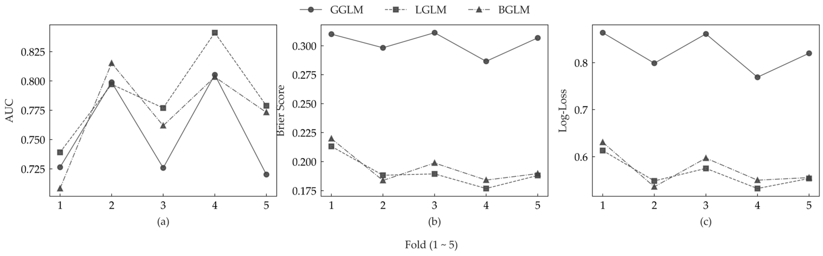
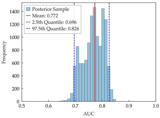
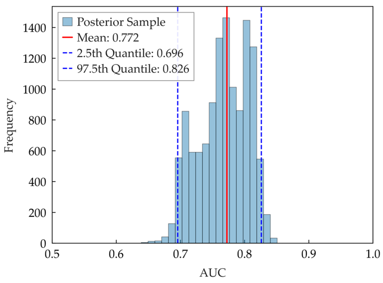
To reduce differences in data across folds in five-fold stratified cross-validation, the same test data are used for both model calculation and evaluation index calculation. The five-fold performance index results for each model, calculated as above, are shown in Figure 5, and Figure 6 shows the AUC posterior distribution of BGLM based on sampling from the sample statistics.

Figure 5. Performance comparison of each fold model under five-fold cross-validation: (a) AUC; (b) Brier Score; (c) Log-Loss.

Figure 6. Posterior distribution of AUC for BGLM.

First, for model effect evaluation, AUC values (Figure 5a) show high overlap, with fold-to-fold fluctuations mainly between 0.72 and 0.82, and all can distinguish liquefaction. LGLM’s AUC is slightly higher than BGLM, and both are higher than GGLM. Brier Score and Log-Loss indicators (Figure 5b,c) change similarly because both measure the deviation between predicted liquefaction rates and actual results, reflecting sensitivity to prediction accuracy errors. Specifically, BGLM and LGLM have scores in a small range (Brier Score between 0.18 and 0.22; Log-Loss between 0.50 and 0.65); by comparison, GGLM shows larger errors and higher losses.

The results show that GGLM still maintains a reasonable sample discrimination capacity on the adopted dataset. Notably, there is a significant discrepancy between its AUC values and the corresponding Brier scores and log losses. This is mainly because the original GGLM lacks targeted optimization using local data. Accordingly, this study attempts to calibrate its intercept term. After calibration, the intercept changes from 8.801 to 13.257. However, both the Brier score and log loss increase rather than decrease, with the Brier score rising from 0.303 to 0.396 and the log loss rising from 0.823 to 1.304. The resultant large prediction errors limit its direct regional application. However, the AUC performance of GGLM after data updating is better than that of the model of Zhu et al. (2017) [10] (AUC = 0.588) applied in the same region. This demonstrates that global liquefaction prediction models have obvious limitations when applied locally. Supplementary geological and seismic data specific to the study area are required for reasonable parameter calibration in practical engineering applications.

LGLM is trained on full local datasets and achieves favorable cross-validation results, yet maximum likelihood estimation carries the risk of overfitting. By contrast, BGLM maintains comparable predictive accuracy and restrains unreasonable parameter variation via global prior constraints, yielding more stable estimation and consistent core parameter significance across samples.

From Figure 6, the 95% HDI of the AUC posterior distribution for BGLM is 0.690–0.826, with a mean of 0.773. The prediction uncertainty reflected by this interval stems from the objective quantification of the parameter posterior distribution by the Bayesian framework on the one hand and may be related to the inherent spatial heterogeneity of the data and the adaptation of the model structure to complex geological conditions on the other hand. This uncertainty is intuitively reflected in the discrete characteristics of posterior samples and the large fluctuations in indicators during five-fold cross-validation.

The results reveal that Bayesian-updated models can output complete AUC distributions and confidence intervals instead of single, fixed, deterministic values, which can effectively reflect prediction uncertainty and avoid underestimating hazard risks, thereby providing more comprehensive information for risk characterization. From the perspective of spatial disaster assessment, integrating GIS and Bayesian methods can better capture the uncertainty hidden in geospatial data, and the superiority of this uncertainty quantification mode over traditional single-point index evaluation has been fully demonstrated in existing research [25]. Such an evaluation mode better fits complex regional geological features and presents predictive variability in a straightforward manner.

4.2. Variable Ablation Analysis

To verify the rationality of simplifying the precipitation variable, variable ablation analysis is conducted by comparing the overall predictive performance between models with and without the precipitation variable. The results are presented in Table 6.

Table 6. Variable ablation analysis of precipitation based on mean performance.

Model	$\mathit{P}\mathit{r}\mathit{e}\mathit{c}\mathit{i}\mathit{p}$ (Y/N)	AUC	Brier Score	Log-Loss	Change
GGLM	Y	0.7554	0.3026	0.8227	Slightly increased error
	N	0.7606	0.3572	0.9915
LGLM	Y	0.7866	0.1911	0.5645	Almost unchanged
	N	0.7878	0.1911	0.5645
BGLM	Y	0.7724	0.1952	0.5738	Almost unchanged
	N	0.7776	0.1949	0.5728

Note: Y = with precipitation variable; N = without precipitation variable. Change represents the performance variation of the model without precipitation relative to that with precipitation.

Table 6 shows that removing the precipitation variable has almost no adverse effect on the performance of LGLM and BGLM. Their AUC values remain stable, with negligible changes in Brier Score and Log-Loss. For GGLM, although the AUC rises slightly after excluding the precipitation variable, the Brier Score and Log-Loss increase substantially, indicating deteriorated probability calibration. In general, regional models, including LGLM and BGLM, exhibit highly consistent predictive performance regardless of whether the precipitation variable is incorporated.

Verified by ablation analysis, $precip$ contributes little to prediction in this study area and can be reasonably simplified or removed for regional liquefaction modeling.

4.3. Spatial Blocking Cross-Validation

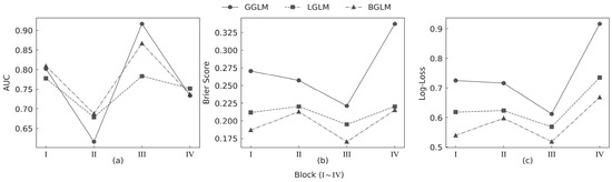
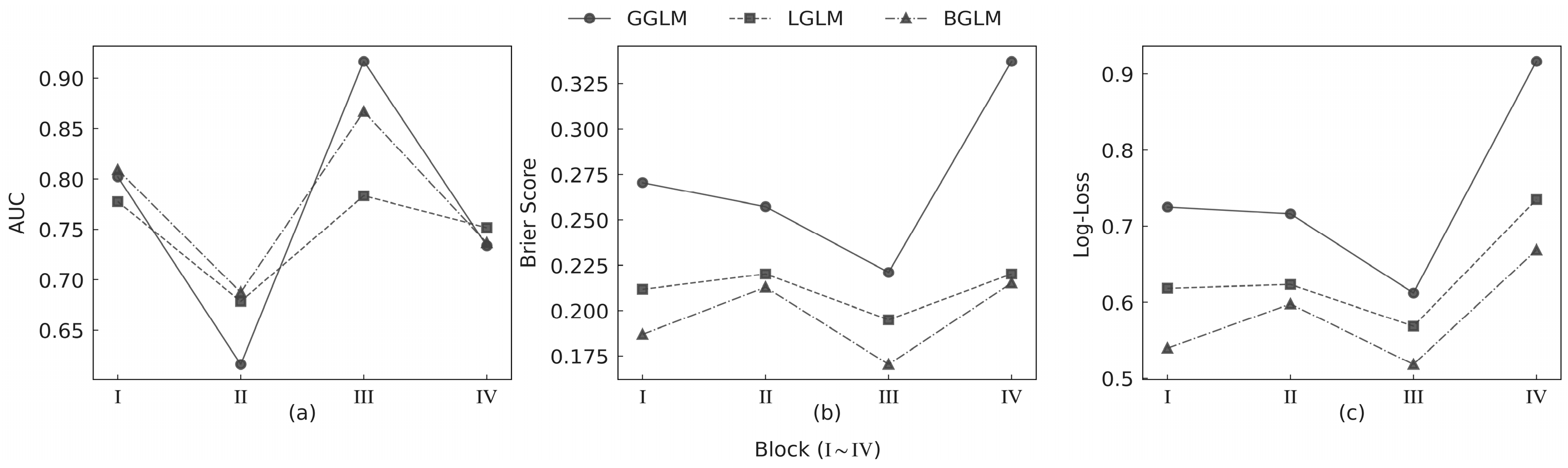
In the above section, stratified five-fold cross-validation was used to ensure balanced sample distribution and to reliably evaluate overall prediction accuracy. To avoid overestimating model performance due to random cross-validation, this section uses spatial blocking cross-validation to account for spatial autocorrelation and reduce optimistic bias induced by random sampling. The standard logistic likelihood is adopted here to maintain consistency with classic geospatial liquefaction models. Based on this strategy, the study area is divided into four spatial blocks (Block I, II, III, IV). Each block is used sequentially as the test set, while the other three serve as the training set to evaluate the model’s regional spatial generalization. The performance metrics (AUC, Brier Score, and Log-Loss) of GGLM, LGLM, and BGLM in each block under spatial blocking cross-validation are presented in Figure 7.

Figure 7. Model performance indicators of three models under spatial blocking cross-validation: (a) AUC; (b) Brier Score; (c) Log-Loss.

Overall, BGLM performs best in predicting different spatial areas. It has the highest average AUC of 0.775 ± 0.068, the lowest Brier score of 0.196 ± 0.019, and the lowest Log-Loss of 0.581 ± 0.058 among the three models. LGLM performs well, with an average AUC of 0.748 ± 0.042, but its Brier score and Log-Loss are higher than those of BGLM. GGLM has a similar average AUC of 0.767 ± 0.109, but its Brier score (0.272 ± 0.042) and Log-Loss (0.743 ± 0.110) are higher, suggesting unreliable predictions and less stable calibration.

For spatial stability, GGLM fluctuates most across blocks, with AUC from 0.616 to 0.917 and a high standard deviation of 0.109, meaning it is sensitive to regional geology and not spatially adaptable. LGLM is steadier but has a higher overall prediction error. BGLM maintains high accuracy and the lowest standard deviations, showing robustness to spatial differences. Its 95% highest posterior density interval for AUC, [0.670, 0.917], quantifies uncertainty and helps clarify uncertainty in regional risk assessment.

Compared with five-fold cross-validation, spatial blocked validation is closer to practical regional extrapolation. LGLM achieves a good fit on known samples, yet its performance drops sharply on unseen spatial data, indicating clear overfitting. By contrast, BGLM maintains stable, reliable performance across different spatial units, demonstrating stronger generalization.

The above results verify that integrating information updating with Bayesian inference effectively promotes the migration and adaptation of global models to this study’s regional scenarios, thereby providing an optimal strategy that balances prediction stability and regional applicability within the study area.

4.4. Discussions

This study performs Bayesian recalibration on the existing geospatial logistic framework and establishes a Bayesian-updated geospatial liquefaction model (BGLM) that integrates global prior information and locally updated geospatial data and validates it using data from the 2008 Wenchuan earthquake. Comparisons with existing similar geospatial liquefaction models further clarify the technical rationale, key differences, and contributions of the proposed approach.

The Global Geospatial Liquefaction Model (GGLM) proposed by Zhu et al. [10] provides a general and standardized framework widely used for post-earthquake rapid assessment. However, the model is dominated by coastal earthquake cases and yields relatively low accuracy when directly applied to inland mountainous areas such as Wenchuan, as validated by Rashidian and Baise [40]. Although the latter validated and improved the GGLM, a generalized regional updating strategy adaptable to different regions was not established. The Bayesian updating method introduced by Engler et al. [21] relies on in situ data such as CPT, which limits its application in data-scarce regions. Baise et al. [26] regionalized the GGLM for California, but their approach relies on dense local liquefaction observations, limiting its applicability.

Table 7 presents a detailed comparison between this study and existing models.

Table 7. Comparison between this study and similar geospatial liquefaction models.

Item	Zhu et al. [10]	Engler et al. [21]	Baise et al. [26]	This Study
Model Type	Global logistic regression model	Geospatial–geotechnical fusion model	Bayesian logistic regression model	Bayesian geospatial model (BGLM)
Bayesian Implementation	No Bayesian	Direct Bayesian probability update	Laplace approximation	MCMC-NUTS sampling
Core Data	27 global earthquakes; global geospatial data	Loma Prieta earthquake + CPT data	9 California earthquakes	Wenchuan earthquake + local $V_{S30}$/$wtd$
Key Method	Maximum likelihood estimation	Fusion with geotechnical LPI	Bayesian update with global prior	Uncertainty quantification & spatial validation
Application	Global	Loma Prieta, USA	California, USA	Wenchuan, China
Key Contribution	Established global liquefaction framework	Integrate geospatial and in situ data	Regionalized Bayesian updating framework	Regionalization + full uncertainty analysis
Limitation	Low accuracy in inland/mountain areas	Depends on dense CPT data	No full uncertainty quantification	Single earthquake case

As shown in the comparison, this study follows a similar technical rationale to existing models, i.e., regional liquefaction prediction using geospatial information. Nevertheless, apparent differences lie in the model framework, the Bayesian algorithm, the data sources, and the research priorities. Some existing models lack regional adaptation, while others require substantial amounts of measured data and a large sample size. Compared with the conventional Laplace approximation, this study adopts MCMC-NUTS sampling to analyze posterior parameter uncertainty and identify key influential factors of liquefaction assessment. By incorporating regional recalibration into the Bayesian framework, the established BGLM achieves favorable regional adaptability in the study area, providing a reference for localizing global models.

While the model achieves decent overall performance, some limitations remain. First, the model is established using data from the Wenchuan earthquake. Because it is restricted to a single seismic event, it cannot fully reflect variations in ground motion and site conditions across diverse scenarios. Second, geospatial proxy indicators are adopted for analysis. The method can support a preliminary rapid liquefaction assessment at the regional scale, but it cannot match the accuracy of borehole and geotechnical test data for detailed site-specific evaluation. Meanwhile, ${\mathrm{V}}_{\mathrm{S}30}$ is calculated as an average over depth, which limits the characterization of subtle features in shallow, thin liquefied soil layers. In addition, only internal cross-validation is conducted in this study. External verification using independent earthquake records and data from new regions is lacking, leaving the model’s generalization performance and engineering-oriented performance analysis to be further explored.

5. Conclusions

Aiming at the insufficient research on global geospatial liquefaction models in China, this study takes the 2008 Wenchuan earthquake as a case study, updates average shear wave velocity ($V_{S30})$ and groundwater table depth ($wtd$) data, and establishes a local model (LGLM) and a Bayesian-updated model (BGLM). The main conclusions are as follows:

(1)

Integrating regional recalibration and the Bayesian inference framework can effectively improve the prediction accuracy, calibration performance, and regional adaptability within the study area of the liquefaction model. Verified by both stratified five-fold and spatial blocking cross-validation, the Bayesian-updated model (BGLM) yields the best overall performance, confirming that the combination of local data refinement and Bayesian inference effectively promotes the migration and adaptation of global models to the regional scenarios of Wenchuan and provides an optimal strategy balancing prediction stability and applicability, as well as a useful reference for the localization of global models.

(2)

The Bayesian framework quantifies both predictive and parametric uncertainty and objectively characterizes model performance variability and reliability bounds. Compared with the traditional single-point AUC metric, the complete posterior distributions and 95% HDIs obtained by the Bayesian-updated model better reflect the variability in practical engineering applications, providing informative support for seismic risk characterization and regional parameter analysis in the study area.

(3)

Bayesian posterior parameter estimation clarifies the importance and contribution of each variable in the study area. $V_{S30}$ and $wtd$ act as dominant contributors, while $\mathrm{P}\mathrm{G}\mathrm{V}$ and $dw$ show stable effects. Verified by ablation analysis, $precip$ has a negligible impact on prediction performance for the Wenchuan earthquake case and can be reasonably simplified or removed in regional liquefaction modeling.

References

- Yuan, J.Y.; Wang, Y.L.; Ma, J.J.; Wu, X.Y.; Yuan, X.M. Study regarding typical liquefaction damage during the 2021 Maduo Ms7.4 earthquake in China. Earthq. Eng. Eng. Vib. 2023, 22, 895–908. [Google Scholar] [CrossRef] [Scilit]
- Yang, Y.S.; Liu, X.S.; Zhao, J.M.; Wang, X.G.; Wen, Y.F.; Chen, N.; Liu, Q.W. Methods for liquefaction potential evaluation of embankment and foundation and discussion on these methods. J. Hydroelectr. Eng. 2011, 30, 90–97+108. (In Chinese) [Google Scholar]
- Seed, H.B.; Idriss, I.M. Simplified procedure for evaluating soil liquefaction potential. J. Soil Mech. Found. Div. 1971, 97, 1249–1273. [Google Scholar] [CrossRef] [Scilit]
- Robertson, P.K.; Campanella, R.G. Liquefaction potential of sands using the CPT. J. Geotech. Eng. 1985, 111, 384. [Google Scholar] [CrossRef] [Scilit]
- Andrus, R.D.; Stokoe, K.H., II. Liquefaction resistance of soils from shear-wave velocity. J. Geotech. Geoenviron. Eng. 2000, 126, 1015–1025. [Google Scholar] [CrossRef] [Scilit]
- Ishac, M.F.; Heidebrecht, A.C. Energy dissipation and seismic liquefaction in sands. Earthq. Eng. Struct. Dyn. 1982, 10, 59–68. [Google Scholar] [CrossRef] [Scilit]
- Yang, H.J.; Liu, Z.K.; Xie, Y.X.; Li, S.M. A probabilistic liquefaction reliability evaluation system based on CatBoost-Bayesian considering uncertainty using CPT and VS measurements. Soil Dyn. Earthq. Eng. 2023, 173, 108101. [Google Scholar] [CrossRef] [Scilit]
- Bozzoni, F.; Bonì, R.; Conca, D.; Meisina, C.; Lai, C.G.; Zuccolo, E. A geospatial approach for mapping the earthquake-induced liquefaction risk at the European scale. Geosciences 2021, 11, 32. [Google Scholar] [CrossRef] [Scilit]
- Farahani, A.; Ghayoomi, M. Soil moisture-based global liquefaction model (SMGLM) using soil moisture active passive (SMAP) satellite data. Soil Dyn. Earthq. Eng. 2024, 177, 108350. [Google Scholar] [CrossRef] [Scilit]
- Zhu, J.; Baise, L.G.; Thompson, E. An updated geospatial liquefaction model for global application. Bull. Seismol. Soc. Am. 2017, 107, 1365–1385. [Google Scholar] [CrossRef] [Scilit]
- Li, C.C.; Li, Z.Y.; Yuan, X.M. Simplified prediction method for regional seismic soil liquefaction. Chin. J. Geophys. 2020, 63, 2084–2095. (In Chinese) [Google Scholar] [CrossRef]
- Brandenberg, S.J.; Zimmaro, P.; Stewart, J.P.; Kwak, D.Y.; Franke, K.W.; Moss, R.E.S.; Çetin, K.Ö.; Can, G.; Ilgac, M.; Stamatakos, J.; et al. Next-generation liquefaction database. Earthq. Spectra 2020, 36, 939–959. [Google Scholar] [CrossRef] [Scilit]
- Geyin, M.; Baird, A.J.; Maurer, B.W. Field assessment of liquefaction prediction models based on geotechnical versus geospatial data, with lessons for each. Earthq. Spectra 2020, 36, 1386–1411. [Google Scholar] [CrossRef] [Scilit]
- Yilmaz, C.; Silva, V.; Weatherill, G. Probabilistic framework for regional loss assessment due to earthquake-induced liquefaction including epistemic uncertainty. Soil Dyn. Earthq. Eng. 2021, 141, 106493. [Google Scholar] [CrossRef] [Scilit]
- Zumpano, V.; Pisano, L.; Filice, F.; Ugenti, A.; de Lucia, D.; Wasowski, J.; Santaloia, F.; Lollino, P. Regional-scale seismic liquefaction susceptibility mapping via an empirical approach validated by site-specific analyses. Geosciences 2022, 12, 215. [Google Scholar] [CrossRef] [Scilit]
- Juang, C.; Zhang, J. Bayesian Methods for Geotechnical Applications—A Practical Guide. In Geotechnical Safety and Reliability; American Society of Civil Engineers: Reston, VA, USA, 2017. [Google Scholar] [CrossRef] [Scilit]
- Shen, M.; Chen, Q.; Zhang, J.; Gong, W.; Juang, C.H. Predicting liquefaction probability based on shear wave velocity: An update. Bull. Eng. Geol. Environ. 2016, 75, 1199–1214. [Google Scholar] [CrossRef] [Scilit]
- Sadik, L.; Khoshnevisan, S. Region-specific CPT-SPT correlations for cohesionless soils: A hierarchical Bayesian approach. Geotech. Geol. Eng. 2025, 43, 430. [Google Scholar] [CrossRef] [Scilit]
- Namikawa, T. Statistical uncertainty on assessment of spatial liquefaction resistance. In Earthquake Geotechnical Engineering for Protection and Development of Environment and Constructions—Proceedings of the 7th International Conference on Earthquake Geotechnical Engineering; Silvestri, F., Moraci, N., Eds.; CRC Press: Boca Raton, FL, USA; Balkema: Leiden, The Netherlands, 2019; pp. 4095–4102. [Google Scholar]
- Choi, I.; Kim, J.H.; Kang, W.H.; Kim, Y. Bayesian framework for updating seismic loss functions with limited observational data in low-to-moderate seismicity regions. J. Earthq. Eng. 2022, 26, 8205–8228. [Google Scholar] [CrossRef] [Scilit]
- Engler, D.T.; Thompson, E.M.; Maurer, B.W.; Jaiswal, K. Updating regional-scale geospatial liquefaction models with locally available geotechnical data. Seismol. Res. Lett. 2025, 96, 3365–3378. [Google Scholar] [CrossRef] [Scilit]
- Zhao, Z.; Duan, W.; Cai, G.; Wu, M.; Liu, S. CPT-based fully probabilistic seismic liquefaction potential assessment to reduce uncertainty: Integrating XGBoost algorithm with Bayesian theorem. Comput. Geotech. 2022, 149, 104868. [Google Scholar] [CrossRef] [Scilit]
- Pirhadi, N.; Hu, J.; Fang, Y.; Jairi, I.; Wan, X.; Lu, J. Seismic gravelly soil liquefaction assessment based on dynamic penetration test using expanded case history dataset. Bull. Eng. Geol. Environ. 2021, 80, 8159–8170. [Google Scholar] [CrossRef] [Scilit]
- Durap, A.; Balas, C.E. Towards sustainable coastal management: A hybrid model for vulnerability and risk assessment. J. Coast. Conserv. 2024, 28, 66. [Google Scholar] [CrossRef] [Scilit]
- Durap, A. Mapping coastal resilience: A Gis-based Bayesian network approach to coastal hazard identification for Queensland’s dynamic shorelines. Anthr. Coasts 2024, 7, 23. [Google Scholar] [CrossRef] [Scilit]
- Baise, L.G.; Shirzadi, H.; Moaveni, B.; Kottke, A. A regionalized geospatial liquefaction model for California. In Geo-Extreme 2025: Geotechnical Earthquake Engineering; American Society of Civil Engineers: Reston, VA, USA, 2025; pp. 128–136. [Google Scholar] [CrossRef] [Scilit]
- Zhang, Y.S.; Lei, W.Z.; Shi, J.S.; Wu, S.R.; Wang, X.L. General characteristics of 5.12 earthquake-induced geohazards in Sichuan. J. Geomech. 2008, 2, 109–116. (In Chinese) [Google Scholar] [CrossRef]
- Zhu, J.; Baise, L.G.; Thompson, E.M. Liquefaction observations from ten earthquakes in the US, Japan, China, and Taiwan. In U.S. Geological Survey Data Release; U.S. Geological Survey: Reston, VA, USA, 2016. [Google Scholar] [CrossRef]
- Youd, T.L.; Idriss, I.M. Liquefaction resistance of soils: Summary report from the 1996 NCEER and 1988 NCEER/NSF workshops on evaluation of liquefaction resistance of soils. J. Geotech. Geoenviron. Eng. 2001, 127, 297–313. [Google Scholar] [CrossRef] [Scilit]
- Kayen, R.; Moss, R.E.S.; Thompson, E.M.; Seed, R.B.; Cetin, K.O.; Der Kiureghian, A.; Tanaka, Y.; Tokimatsu, K. Shear-wave velocity-based probabilistic and deterministic assessment of seismic soil liquefaction potential. J. Geotech. Geoenviron. Eng. 2013, 139, 407–419. [Google Scholar] [CrossRef] [Scilit]
- Wald, D.J.; Allen, T.I. Topographic slope as a proxy for seismic site conditions and amplification. Bull. Seismol. Soc. Am. 2007, 97, 1379–1395. [Google Scholar] [CrossRef] [Scilit]
- Zhou, J.; Li, L.; Li, X.J.; Xi, N.; Tian, X. A 30 arcsec resolution VS30 map for mainland China using refined topographic slope-based cokriging (SCK) model. Bull. Seismol. Soc. Am. 2025, 115, 332–348. [Google Scholar] [CrossRef] [Scilit]
- Fan, Y.; Li, H.; Miguez-Macho, G. Global patterns of groundwater table depth. Science 2013, 339, 940–943. [Google Scholar] [CrossRef] [Scilit]
- European Committee for Standardization. Eurocode 8: Design of Structures for Earthquake Resistance; European Committee for Standardization: Brussels, Belgium, 2004. [Google Scholar]
- ASCE/SEI 7-10; Minimum Design Loads for Buildings and Other Structures, 3rd Printing, Revised Commentary. American Society of Civil Engineers: Reston, VA, USA, 2013.
- Verdugo, R. Seismic site classification. Soil Dyn. Earthq. Eng. 2019, 124, 317–329. [Google Scholar] [CrossRef] [Scilit]
- Boore, D.M.; Stewart, J.P.; Seyhan, E.; Atkinson, G.M. NGA-West2 equations for predicting PGA, PGV, and 5% damped PSA for shallow crustal earthquakes. Earthq. Spectra 2014, 30, 1057–1085. [Google Scholar] [CrossRef] [Scilit]
- Kongar, I.; Rossetto, T.; Giovinazzi, S. Evaluating simplified methods for liquefaction assessment for loss estimation. Nat. Hazards Earth Syst. Sci. 2017, 17, 781–800. [Google Scholar] [CrossRef] [Scilit]
- Zhu, J.; Daley, D.; Baise, L.G.; Thompson, E.M.; Wald, D.J.; Knudsen, K.L. A geospatial liquefaction model for rapid response and loss estimation. Earthq. Spectra 2015, 31, 1813–1837. [Google Scholar] [CrossRef] [Scilit]
- Rashidian, V.; Baise, L.G. Regional efficacy of a global geospatial liquefaction model. Eng. Geol. 2020, 272, 105644. [Google Scholar] [CrossRef] [Scilit]
- Durap, A.; Balas, C.E.; Çokgör, Ş.; Balas, E.A. An Integrated Bayesian Risk Model for Coastal Flow Slides Using 3-D Hydrodynamic Transport and Monte Carlo Simulation. J. Mar. Sci. Eng. 2023, 11, 943. [Google Scholar] [CrossRef] [Scilit]
- Zhan, W.W.; Baise, L.G.; Moaveni, B. An uncertainty quantification framework for logistic regression based geospatial natural hazard modeling. Eng. Geol. 2023, 324, 107271. [Google Scholar] [CrossRef] [Scilit]
- Gelman, A.; Carlin, J.; Stern, H.; Dunson, D.; Vehtari, A.; Rubin, D. Bayesian Data Analysis, 3rd ed.; CRC Press: Boca Raton, FL, USA, 2013. [Google Scholar]
Disclaimer/Publisher’s Note: The statements, opinions and data contained in all publications are solely those of the individual author(s) and contributor(s) and not of MDPI and/or the editor(s). MDPI and/or the editor(s) disclaim responsibility for any injury to people or property resulting from any ideas, methods, instructions or products referred to in the content. |
© 2026 by the authors. Licensee MDPI, Basel, Switzerland. This article is an open access article distributed under the terms and conditions of the Creative Commons Attribution (CC BY) license.