Slope Stability Prediction Based on CCO-Optimized XGBoost Model

Abstract

Achieving rapid and accurate prediction of slope stability is a key scientific issue in slope engineering. However, slope stability is governed by multi-factor coupling effects and exhibits strong nonlinear characteristics, and traditional slope stability prediction methods have clear limitations in predicting the stability of complex slope engineering. To address such problems, a CCO-optimized XGBoost model for slope stability prediction is constructed by using the Cuckoo Catfish Optimizer (CCO) to optimize the hyperparameters of XGBoost, thereby enhancing prediction accuracy and robustness. Based on 832 slope cases covering various slope engineering scenarios, six key feature parameters—slope height (H), slope angle (β), unit weight (γ), cohesion (C), internal friction angle (φ), and pore pressure ratio (r_u)—were selected to construct the dataset. Ten-fold cross-validation was adopted for model training and robustness testing. After optimization, the optimized model achieved an accuracy of 0.898, precision of 0.892, recall of 0.902, F1-score of 0.897, and AUC of 0.944, representing its optimal comprehensive performance. These evaluation metrics are significantly better than those of unoptimized XGBoost, RandomForest, LightGBM, and the representative PSO-XGBoost model. The SHAP analysis method was used to improve the interpretability of model predictions. Prediction analysis was carried out using 12 sets of real engineering cases, and the prediction results were consistent with the actual conditions, further verifying the model’s generalization ability. This model shows favorable performance in slope stability prediction and can provide a reference method for slope stability evaluation, decision optimization and risk prevention and control in slope engineering.

1. Introduction

Slope stability is one of the core topics in the fields of geotechnical engineering and engineering geology, and it is directly related to the safe operation and economic benefits of major projects such as mining and transportation. Once slope instability occurs, the risk spillover range is wide and the consequences are severe [1]. Therefore, constructing a high-precision, generalizable, and interpretable rapid slope stability assessment method oriented to engineering applications has important theoretical significance and practical value. It can enable rapid evaluation of slope stability under complex working conditions, thereby providing reliable support for engineering decision-making and disaster prevention and control.

Traditional slope stability prediction methods mainly include the limit equilibrium method and the strength reduction method. These methods have clear mechanical foundations and are supported by standardized systems; to a certain extent, they can characterize slope failure mechanisms and provide safety factors or instability mode judgments for engineering design [2]. However, traditional methods still face challenges such as insufficient adaptability under complex geology and multi-working-condition scenarios, strong dependence on preset slip surfaces, insufficient fusion of real-time monitoring data, and difficulty in multi-physics coupling analysis. With the development of monitoring and informatization methods, the capability of acquiring and accumulating slope data has significantly improved, promoting the continuous development of prediction methods centered on machine learning. These provide important supplements to traditional analysis methods, especially for handling strong nonlinearity, multi-factor coupling, and rapid inference with large samples. Therefore, their use in engineering practice has become increasingly widespread.

Regarding the application of machine learning in slope stability prediction, extensive achievements have been made in research at home and abroad. Early work mostly used models such as neural networks and support vector machines to perform stable/unstable discrimination or safety factor regression prediction, showing good fitting ability under certain data scales and feature conditions [3]. Subsequently, ensemble models such as random forests and gradient boosting have been widely applied due to their ability to characterize nonlinear relationships, adapt to mixed features, and provide strong generalization performance. Related studies generally show that tree-model ensembles have relatively stable overall performance on engineering data. Zhang Jiantao et al. proposed a hybrid model, WOA-RF, which significantly improved the accuracy and generalization performance of slope stability prediction by optimizing hyperparameters, achieving efficient computation speed on large-scale engineering datasets [4]. Kurnaz et al. used the AutoGluon framework to develop an AutoML-based slope stability prediction model; by comprehensively comparing the performance of ensemble learning, gradient boosting, and traditional machine learning algorithms, prediction accuracy was significantly improved [5]. Zhang Wengang et al. proposed an XGBoost-based slope stability prediction model; through grid search and cross-validation, they finely optimized hyperparameters and significantly improved interpretability; and using the model’s feature-importance evaluation function, they clearly revealed key factors affecting slope stability [6]. Recently, research has further shifted to directions such as improving cross-scenario transferability, characterizing uncertainty, and enhancing model interpretability. For example, Shan Lin et al. compared the performance of AdaBoost, GBM, ET (Extra Trees), Bagging and other models on different slope datasets, verifying the advantages of ensemble learning algorithms in classification performance and robustness [7]. In the above studies, gradient boosting ensemble models, by virtue of their excellent performance in adaptive parameter optimization and generalization ability, have become widely favored methods in slope stability evaluation.

Although existing studies have promoted the development of slope stability prediction, the ensemble learning model XGBoost remains highly sensitive to hyperparameter settings. Traditional tuning methods (such as grid search and commonly used meta-heuristic algorithms) still suffer from issues of low efficiency and high computational cost. Additionally, these methods often lack sufficient global search capabilities in high-dimensional hyperparameter spaces, with a significant probability of converging to local optima, thereby limiting the model’s performance ceiling and stability under complex working conditions [8,9]. Meanwhile, slope samples exhibit strong heterogeneity, and the generalization ability of most models struggles to meet engineering requirements. As a novel meta-heuristic algorithm, the Cuckoo Catfish Optimizer (CCO) demonstrates superior global search capabilities and convergence efficiency, yet it has not been fully exploited to optimize XGBoost for slope stability prediction.

In view of the above, this paper proposes a CCO-optimized XGBoost model (CCO-XGBoost) for slope stability prediction, which optimizes the hyperparameters of XGBoost by using the Cuckoo Catfish Optimizer (CCO). As a meta-heuristic algorithm inspired by symbiosis and competition behaviors in nature, CCO enhances global optimization ability in high-dimensional search spaces through mechanisms such as “global exploration and local exploitation, chaotic perturbation, death and regeneration.” The aim is to improve hyperparameter search efficiency and reduce the risk of falling into local optima, thereby improving the accuracy and robustness of the XGBoost model in slope stability discrimination tasks, and at the same time, this model reveals the multi-factor nonlinear coupling mechanism through a data-driven approach and offers quantitative insights and engineering decision-making references that are difficult to obtain efficiently via traditional mechanical analysis methods.

2. Data Selection and Dataset Construction

2.1. Feature Data Selection

Selecting appropriate evaluation indicators as features is key to accurately characterizing the target system. Slope stability is affected by many factors, such as topography and geomorphology, geological structures, lithological characteristics, and hydrological conditions. Therefore, slope stability is a complex problem influenced by the coupling of multiple internal and external factors [10].

According to extensive engineering practice and theoretical analysis, the dominant factors affecting slope stability can be summarized as physical and mechanical parameters, slope geometry, and hydrological conditions [11]. Among them, slope height (H) and slope angle (β) determine the geometric form of the slope and are key parameters influencing sliding tendency and potential slip surface shape; unit weight (γ), cohesion (C), and internal friction angle (φ) reflect the physical properties and strength characteristics of the rock/soil mass and directly determine its shear strength and stability capacity; and the pore pressure ratio (r_u) changes the effective stress state of the soil mass, thereby indirectly weakening the shear resistance of the slope [12], and has a significant influence on slope stability.

To establish a reliable prediction model, based on relevant research results at home and abroad and case data under various engineering backgrounds [13,14,15,16], this paper comprehensively collected multi-source slope stability sample data, including engineering measured cases from multiple countries such as China and the United States and some finite element simulation data, covering diverse geological conditions, slope morphologies and hydrological conditions with good data representativeness. Considering the inherent measurement errors of some geotechnical parameters in actual engineering measurements, during data compilation, not only were some duplicate data deleted, but parameter rationality verification was also conducted on the samples, effectively reducing the interference of measurement deviations with model training, and a dataset containing 832 samples was constructed. Among them, there are 421 stable cases and 411 unstable cases; partial data are shown in

Table 1. Slope Sample data.

No.	H/(m)	β/(°)	γ/(KN/m3)	C/(kPa)	φ/(°)	ru/(kPa)	Stability
1	8.00	20.00	18.00	5.00	30.00	0.30	Stable
2	76.80	31.01	21.47	6.90	30.02	0.38	Unstable
3	12.80	27.98	21.78	8.55	32.00	0.49	Unstable
4	511.00	41.00	27.30	10.00	39.00	0.25	Stable
…
829	262.40	47.50	31.30	68.59	37.00	0.25	Unstable
830	51.48	42.72	26.62	31.78	0	0.40	Unstable
831	319.21	43.46	30.00	34.57	27.38	0.27	Unstable
832	25.00	40.00	20.00	35.00	30.00	0.29	Stable

(the dataset is available in the Supplementary Materials). To ensure representativeness and generalization ability for model training, the dataset was randomly reshuffled and then divided into a training set and a test set. Statistical analysis and distribution visualization were conducted for each feature variable to reveal its dispersion and central tendency. This dataset covers slope types under various geological and structural conditions, providing a solid data foundation for subsequent construction and optimization of machine learning models.

2.2. Dataset Features and Correlation Analysis

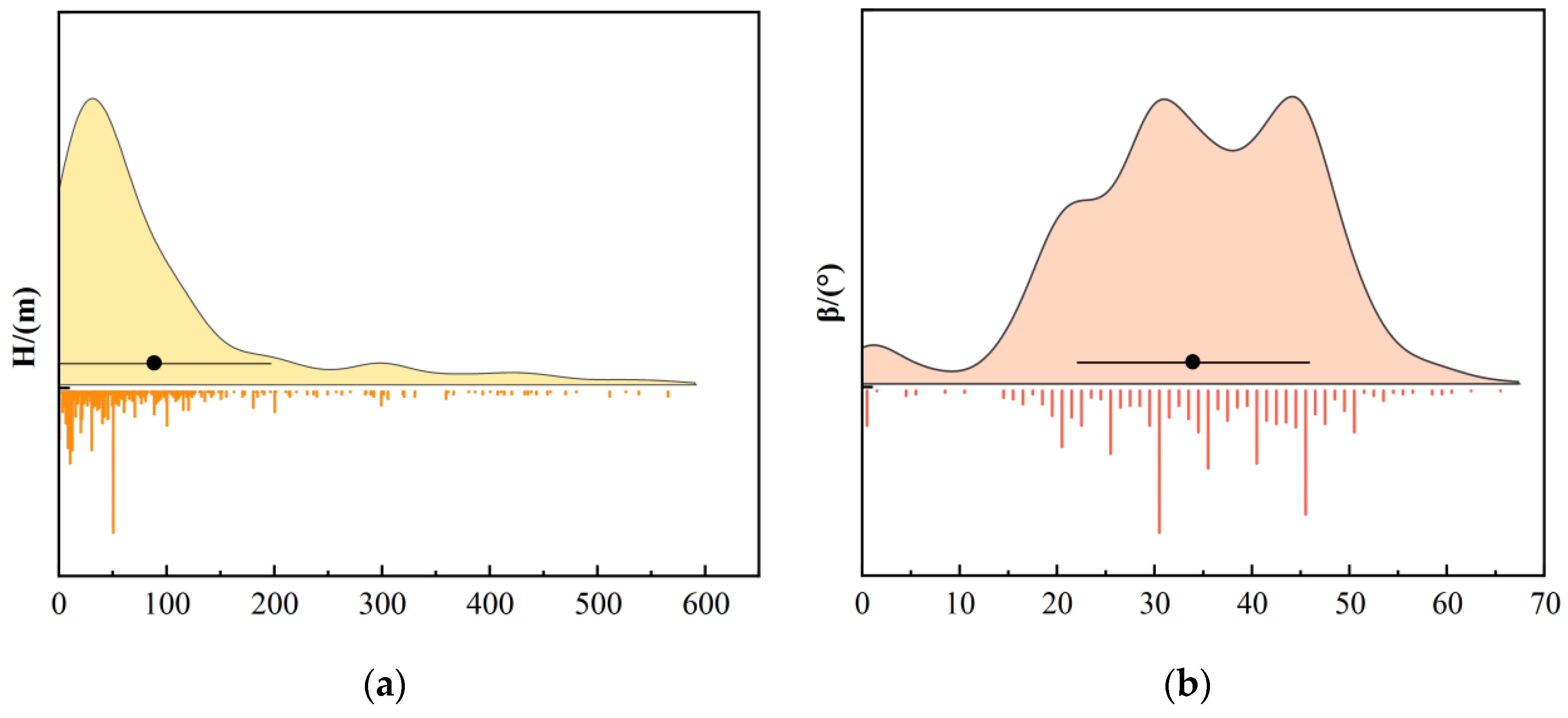
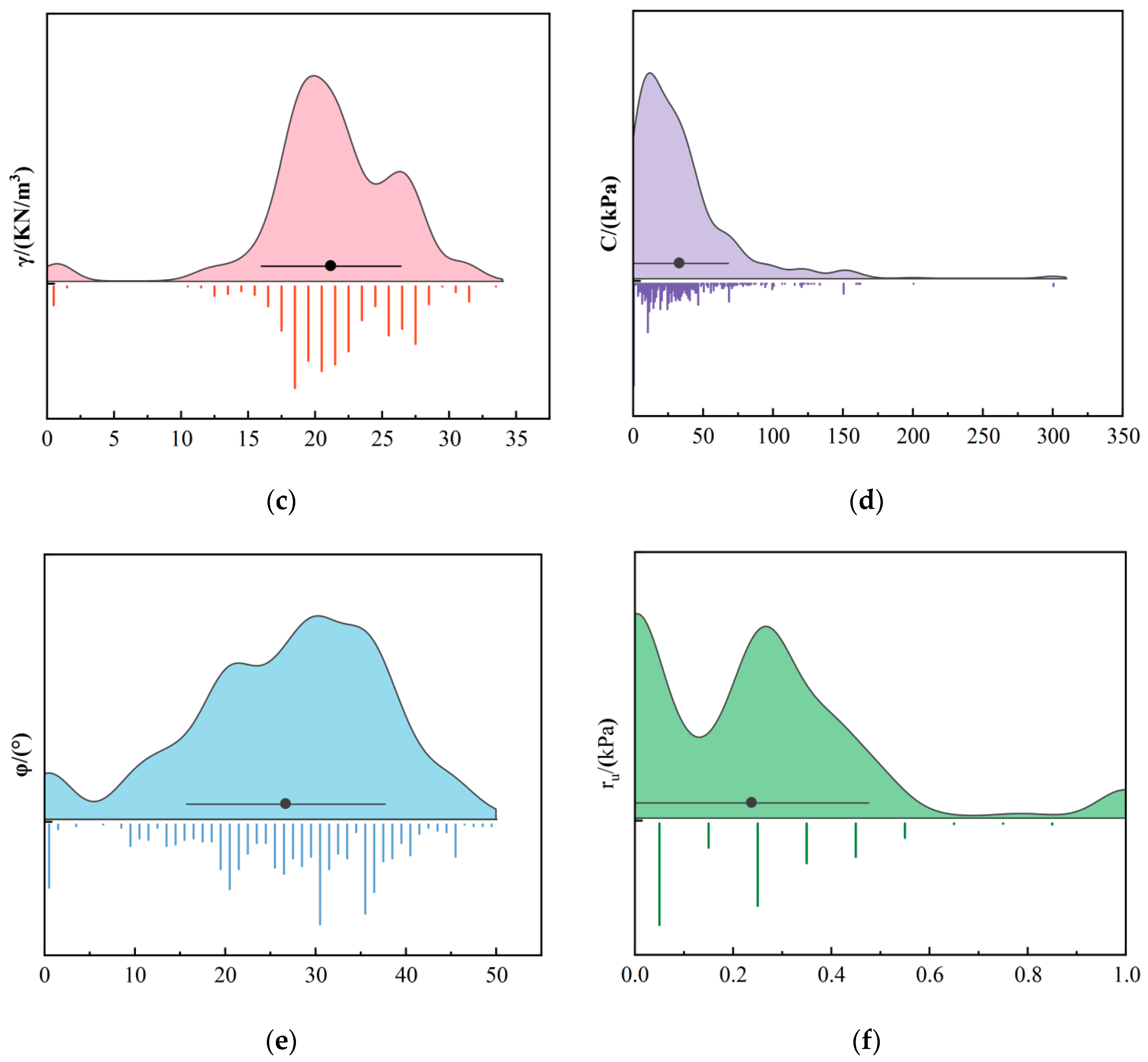
The feature and distribution plots of each parameter are shown in Figure 1: the upper part of each subplot is the value density distribution (a wider contour indicates more concentrated samples), and the lower part is the distribution of individual data points, used to depict the influence across different value ranges. Overall, slope height and cohesion both show a long tail distribution with dense low values and extension to high values, indicating that the samples are mainly low and medium-height slopes and low cohesion, while also including some high and ultra-high slopes and high-cohesion situations; the pore pressure ratio is mainly concentrated in the low-value range but has some scattered high-value points, reflecting working conditions covering low pore pressure to relatively high pore pressure. The internal friction angle shows a unimodal, nearly symmetric, approximately normal distribution, with stronger concentration, while the distributions of angle of slope and unit weight are more gradual and cover a wider range, indicating that the dataset includes a variety of slope shapes and different material density characteristics. Considering the above features, the dataset covers various slope types (such as soil slopes, rock slopes, and composite slopes) and different hydrological and mechanical conditions, which is helpful for the robustness and generalization ability of the model.

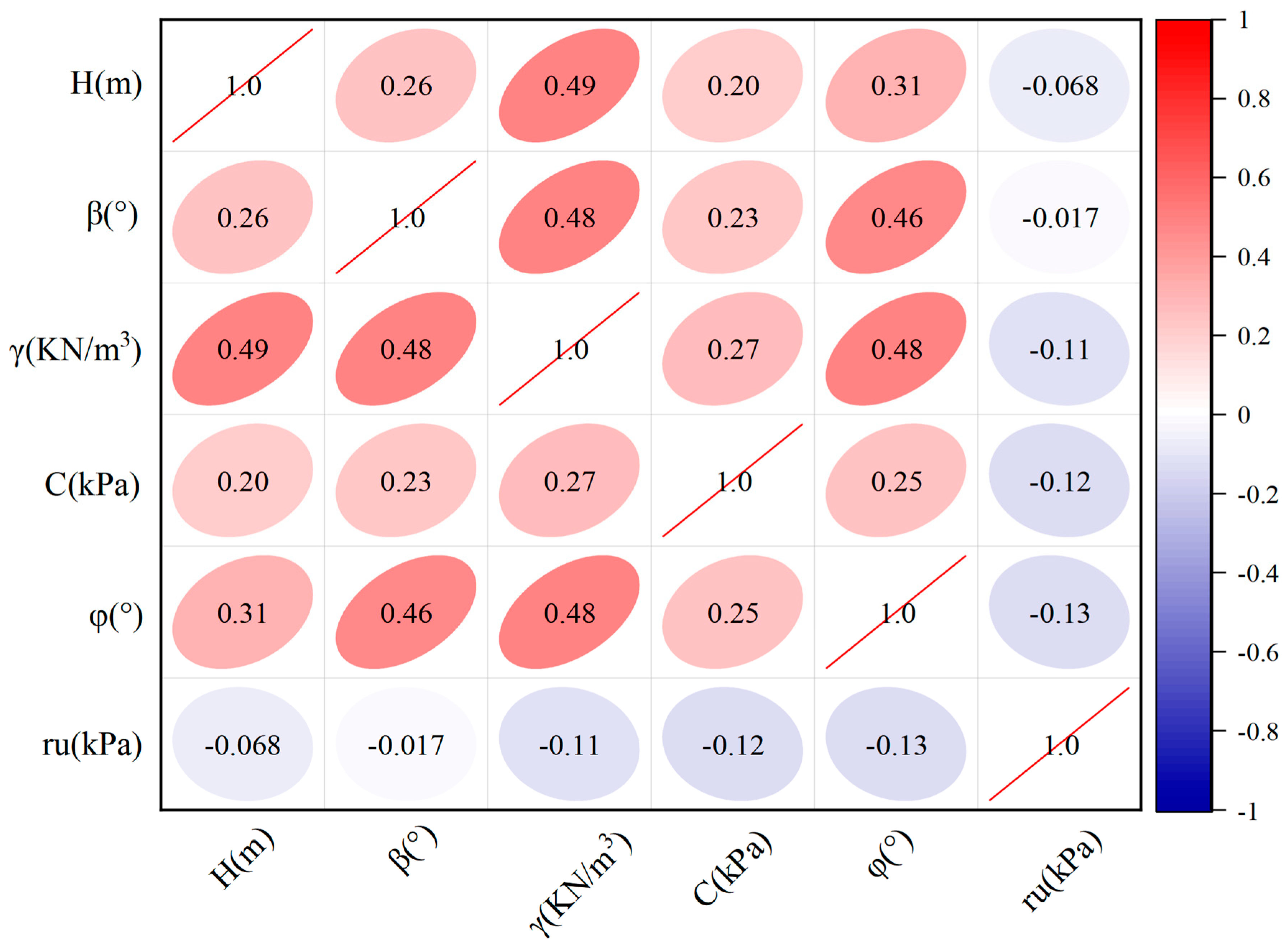
In the design process of slope stability prediction models, it is necessary to first test the interrelationships among sample parameters to avoid multicollinearity problems. Correlation between variables can be measured by comparing their changing trends. The Pearson correlation coefficient is in the range of [−1, 1]. The closer the absolute value of this coefficient is to 1, the stronger the correlation between variables; the closer it is to 0, the weaker the correlation [17]. This coefficient is obtained by standardizing the covariance (the degree to which two variables deviate from their respective means and change synchronously), and it is used to measure the linear correlation between the two. If the coefficient is positive, it indicates positive correlation; if negative, it indicates negative correlation. Usually, the correlation strength corresponding to the absolute value can be divided into: 0–0.3 negligible correlation, 0.3–0.5 low correlation, 0.5–0.8 moderate correlation, and above 0.8 strong correlation. As shown in Figure 2, among the six selected features, the correlation coefficient between unit weight and slope height is the highest, at 0.49. However, the absolute values of correlation coefficients among all features are below 0.5, indicating that there is no significant linear correlation among features. In summary, the features selected in this study are reasonable, and no additional dimensionality reduction or other correlation processing is required.

3. Model Construction

3.1. Algorithm Principles

3.1.1. XGBoost Principles

XGBoost is a scalable machine learning algorithm based on gradient tree boosting [18]. Its core is to iteratively construct an additive tree ensemble model in function space: in round t, on the basis of the fixed existing model, only a new tree is learned to maximize the decrease in the overall objective function, thereby gradually correcting residuals and continuously improving performance. To improve the computability and efficiency of each round of optimization, XGBoost performs a second-order approximation of the loss function at the current prediction point, and uses the first- and second-order gradients of samples as key statistics: given a tree structure, the leaf output is determined by gradient statistics within the leaf; during tree growth, candidate split gain can be calculated by aggregating gradient statistics of left and right child nodes, and then a top-down greedy strategy is used to select the best split, stopping growth when gain is insufficient or complexity constraints are met.

To enhance generalization ability, XGBoost introduces regularization penalties on tree complexity at the objective level, combines shrinkage (learning rate reduction) to limit the update magnitude per round, and uses feature column sampling to reduce variance and improve parallel efficiency. In split point search, it supports both exact and approximate strategies: exact greedy enumerates split points through feature sorting; the approximate strategy constructs candidate splits via quantiles and performs binning search, combined with global candidates and local re-proposal mechanisms to balance accuracy and computational cost, and further proposes a weighted quantile sketch to efficiently obtain candidate quantiles, adapting to sample weights and distributed scenarios. For missing and sparse data, it uses sparsity-aware splitting: by learning the default direction for missing values and only traversing non-missing entries, it achieves unified processing of missing and sparse features and near-linear complexity.

Due to its efficient gradient boosting method, regularization techniques, and strong ability to handle nonlinear relationships, XGBoost can provide high precision results in slope stability prediction [19]. This algorithm can not only handle complex relationships between features and target variables but also has good computational efficiency and strong model generalization ability, and is especially suitable for modeling and prediction on large-scale data.

3.1.2. CCO Algorithm Principles

CCO is a novel meta-heuristic optimization algorithm [20]. Via the multi-strategy collaboration of global exploration, staged perturbation, dynamic update and population regeneration, it provides more efficient, stable and local-optimum-resistant hyperparameter optimization for various prediction models.

In the exploration stage, a wide-range global search is adopted to expand the hyperparameter search boundary, avoid missing optimal parameters due to limited optimization ranges, and improve the rationality of model parameter configuration. The position update formula of the individual is as follows:

$$X_i^{new}=X_i+Z_1\times \left|r_d\right|\times ({\displaystyle \frac{X_{best}+X_{r1}}{2}}-X_{r2})+r_3\times {\displaystyle \frac{1}{2}}\times (X_{r3}-X_{r4})$$

(1)

where $X_{best}$ is the position of the current optimal solution; $X_{r1}$~$X_{r4}$ are randomly selected individual positions; and $r_d$ is a random factor representing cooperation intensity.

In the transition stage, CCO divides the population into two parts, which respectively carry out local fine exploitation and global extended search, balancing optimization efficiency and parameter search depth, enabling the model to rapidly identify high-quality parameters, and taking into account both convergence speed and optimization effect. The update formula is:

$$X_i^{new}=X_i+F\times R_1\times (X_{best}-X_i)$$

(2)

where $F$ is direction factor, ranging in [−1, 1]; $R_1$ is a random factor used to control the moving direction of individuals.

In the exploitation stage, a dynamic perturbation mechanism is introduced to accelerate the convergence of optimal parameters, avoid model performance limitations caused by optimization stagnation, and further improve the efficiency of parameter optimization. The update formula is:

$$X_i^{new}=X_{best}\times (1+T_5\times C_y\times E)+F\times S\times (X_{best}-X_{\mathrm{i}})$$

(3)

where $T_5$ is a constant controlling the intensity of predation perturbation; $C_{\mathrm{y}}$ is the chaos coefficient used to simulate the disturbance to prey during predation.

When an individual stagnates in iteration, the regeneration mechanism is triggered to generate new individuals randomly and escape local optima, thus avoiding low accuracy and poor generalization due to insufficient optimization. The update formula is:

$$X_i^{new}=r_1\times (U_p-Low)+Low$$

(4)

where $U_p$ and $L\mathrm{ow}$ are the upper and lower bounds, respectively, allowed for each decision variable in the search space; $r_1$ is a random variable that determines the generation range of the new individual.

Through the above strategies, the CCO algorithm can significantly improve the hyperparameter optimization quality of the prediction model. Conventional meta-heuristic optimization algorithms mostly adopt classic iterative frameworks, with mature theories and wide applicability, but lack the capacity to dynamically balance global exploration and local exploitation in high-dimensional hyperparameter optimization. The CCO algorithm restructures the population iteration logic, integrates multiple strategies, and forms an optimization architecture fundamentally different from traditional algorithms. It achieves targeted innovations at the optimization mechanism level, better adapts to the high-dimensional hyperparameter optimization requirements for slope stability prediction, and thereby improves the prediction accuracy and operational stability of the model.

3.1.3. CCO Optimized XGBoost Principles

XGBoost performance is highly sensitive to hyperparameter configuration, while traditional tuning methods such as grid search and random search generally have defects such as low optimization efficiency, slow convergence speed, and easy falling into local optima in some scenarios. To address these defects, introducing swarm-intelligence meta-heuristic algorithms with stronger global search ability is practically necessary.

As an emerging swarm-intelligence optimization method, CCO’s optimization of XGBoost covers the entire chain of “hyperparameters–features–tree structure–ensemble strategy”. Its core value lies in using the global search ability of swarm intelligence to compensate for the deficiencies of XGBoost’s local greedy optimization [21]. On the one hand, the adaptive balance between exploration and exploitation accelerates local convergence while maintaining global coverage; on the other hand, chaotic perturbation and population update mechanisms reduce the sensitivity of optimization results to data distribution fluctuations (such as noise, missing values, etc.), enabling stable performance under different data conditions. This indicates that the method has good robustness in complex model optimization tasks. Compared with traditional optimization algorithms, the dynamic exploration–exploitation mechanism of CCO is more suitable for the high-dimensional hyperparameter tuning scenario of XGBoost, which can avoid premature convergence and insufficient optimization in hyperparameter search, and fundamentally improve the optimality of hyperparameter combinations and the generalization ability of the model.

Leveraging the multi-stage optimization mechanism, for different types of slope parameters, the optimization effect of CCO-XGBoost is significant and shows differences. For geometric control variables such as slope height and slope angle, the optimized model is more sensitive to stability responses caused by morphological changes, helping to more accurately characterize the nonlinear relationship between geometry and instability risk; for geotechnical mechanical parameters such as unit weight, cohesion, and angle of internal friction, CCO influences split selection and node partitioning, enabling the model to more effectively express nonlinear responses of each parameter’s variation to stability discrimination; and for hydrological parameters with stronger uncertainty such as pore water pressure, chaotic perturbation and global search mechanisms significantly improve the model’s robustness and generalization ability to input fluctuations and noise, thereby enhancing the stability and reliability of prediction results under different hydrogeological conditions.

3.2. Construction of the CCO-XGBoost Model

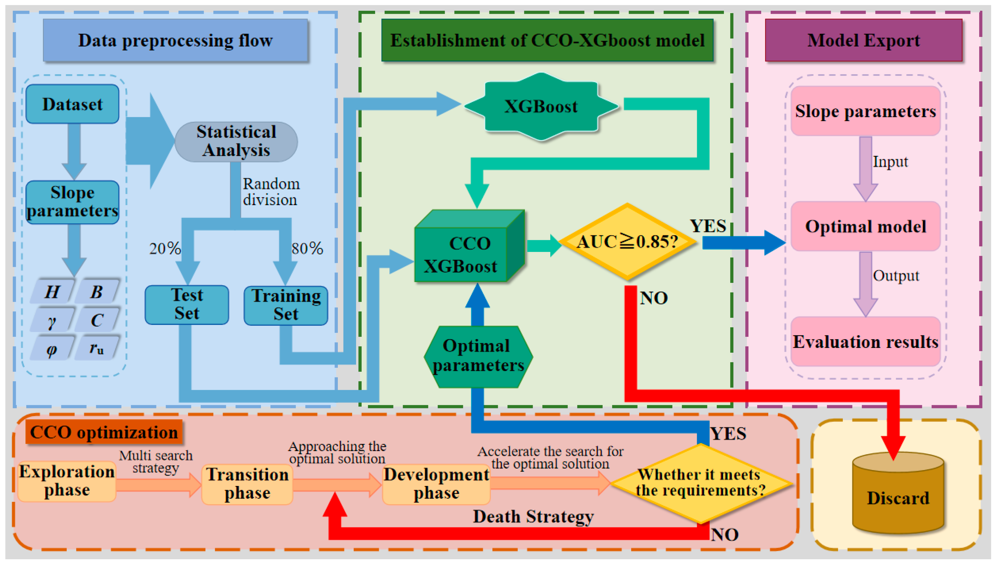
To achieve rapid and accurate prediction of slope stability and ensure stability with interpretability, this paper constructs the CCO-XGBoost model. The model construction and optimization process is shown in Figure 3.

The process is as follows:

(1) Slope stability prediction is a supervised classification problem. Such tasks require learning the mapping relationship between features and target values to build a model. Therefore, the dataset is randomly divided into a training set (80%) and a test set (20%) [22]. The training set is used for model learning and training, while the test set is completely isolated and only used for final generalization ability evaluation to avoid data leakage. The classification variable representing slope stability status is encoded as numerical labels (stable = 1, unstable = 0).

(2) On this basis, XGBoost is used as the base learner to establish a binary classification prediction framework for stability, forming a mapping relationship from input parameters to stability discrimination results, providing a unified model carrier for subsequent parameter optimization and prediction output.

(3) CCO is introduced to optimize the hyperparameters of the XGBoost. The entire optimization process is completed only within the training set, while the test set is completely isolated and does not participate in the optimization process. The CCO optimization is configured with population size (30) and maximum iteration number (50). The hyperparameter search space is determined according to the characteristics of slope engineering data and verified by multiple sets of pre-experiments, covering the number of iterations (150–1000), tree depth (3–6), learning rate (0.01–0.1), subsampling rate (0.75–0.9), feature sampling rate (0.75–0.9), and dynamically adjusting the classification threshold range (0.35–0.8). The scale_pos_weight parameter is adopted to effectively address the problem of sample imbalance. Meanwhile, leveraging the Levy flight strategy and multi-stage search mechanism of the CCO algorithm, it adapts to the high-dimensional parameter space of XGBoost with dynamic search logic and realizes targeted hyperparameter optimization. In the iterative optimization process, search efficiency and convergence stability are improved through multi-strategy updating and inferior solution elimination (discard) mechanism. The above intervals can sufficiently cover the optimal parameter ranges of the model, and exceeding this range tends to cause overfitting, slow convergence and other phenomena. Within this interval, CCO can stably obtain high-performance hyperparameter combinations.

(4) In each iteration, candidate hyperparameters are input into XGBoost for training. The trained model is evaluated on an independent test set using key performance metrics. Since the slope stability dataset suffers from class imbalance, AUC (Area Under Curve) is more robust to unbalanced data and can comprehensively reflect the discriminative ability of the model. Therefore, AUC is taken as the main optimization metric [23]. When AUC meets the threshold requirement (e.g., AUC ≥ 0.85), the optimal parameters are determined and the optimal model is output; otherwise, enter the discarding branch and return to CCO to continue iterations until the criterion is satisfied or the termination condition is reached. In addition, 10-fold cross-validation is carried out within the training set to evaluate model stability and ensure generalizability and robustness.

(5) Finally, export the optimal CCO-XGBoost model, and input slope parameters into the model to obtain stability prediction and evaluation results, thereby realizing discrimination output for slope stability.

3.3. Model Operating Environment

All modeling, training and validation work is implemented in the Python 3.10 environment. The hardware is equipped with an AMD processor and 16 GB of RAM, running a 64-bit Windows operating system. To ensure a fair and rigorous model comparison, all models follow unified parameter tuning rules and perform parameter optimization under identical computing resource conditions. Meanwhile, random seeds are fixed to guarantee the reproducibility of experimental results.

4. Model Performance Evaluation and Result Analysis

4.1. Performance Evaluation Metrics

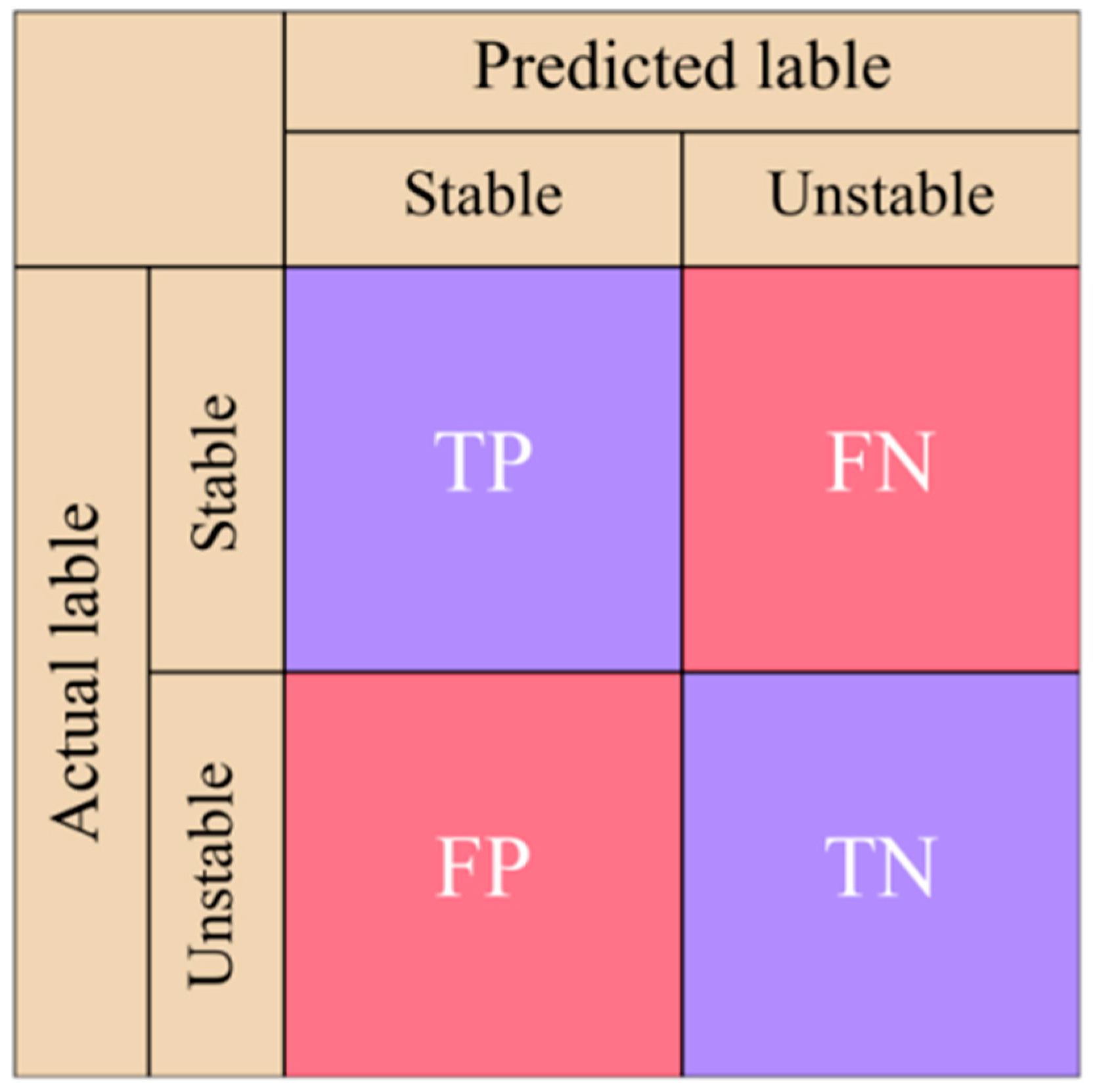
The confusion matrix is a commonly used tool for evaluating classification model performance; it measures model accuracy by summarizing the correspondence between model predictions and actual conditions. In binary classification problems, the confusion matrix contains four basic elements: true positive (TP), false positive (FP), true negative (TN), and false negative (FN) [24]. A schematic diagram of the confusion matrix is shown in Figure 4. In this paper, stable slope is defined as the positive class, and unstable slope is defined as the negative class. The sum of the above four types of sample numbers equals the total number of samples used.

Accuracy is defined as the ratio of the number of samples correctly predicted by the model to the total number of samples, i.e., the proportion of correctly classified samples. Precision is defined as the fraction of samples predicted as positive (i.e., labeled “stable slopes”) that are true positives, reflecting the risk of false alarms (i.e., false positives) produced by the model when predicting failure cases. Recall represents, among all actual positive samples, the proportion correctly identified by the model, reflecting the model’s tolerance for missed reports (i.e., false negatives), and is closely related to the false negative rate. The F1-Score is the harmonic mean of precision and recall and can balance the two; it is especially suitable for classification tasks with imbalanced class distributions and provides a more robust, comprehensive performance evaluation [25].

The AUC value refers to the area enclosed under the receiver operating characteristic (ROC) curve, and it is used to quantify the model’s ability to distinguish positive and negative classes under different classification thresholds. The closer the AUC value is to 1, the stronger the model’s discriminative ability between “stable slope” and “unstable slope”; conversely, an AUC close to 0.5 indicates that the model performance is close to random guessing.

The above evaluation metrics are calculated based on the confusion matrix and ROC curve. The specific formulas are as follows:

$$Accuracy={\displaystyle \frac{TP+TN}{TP+TN+FP+FN}}$$

(5)

$$Percision={\displaystyle \frac{TP}{TP+FP}}$$

(6)

$$Recall={\displaystyle \frac{TP}{TP+FN}}$$

(7)

$$F1={\displaystyle \frac{2Precision\times Recall}{Precision+Recall}}$$

(8)

where TP is the true positive; FP is the false positive; TN is the true negative; and FN is the false negative.

To verify the superiority of the CCO-XGBoost optimized model, three baseline models, including RandomForest, LightGBM and unoptimized XGBoost, and the PSO-XGBoost model constructed by Particle Swarm Optimization (PSO) [26], a commonly used meta-heuristic algorithm in slope engineering, were selected as typical meta-heuristic optimization models for comparative experiments. All models were trained and tested on the same dataset, with 80% as the training set and 20% as the test set. In addition, 10-fold cross-validation was used to ensure model stability and reliability.

In 10-fold cross-validation, the training set is equally divided into 10 subsets. In each iteration, 9 subsets are used for model training, and the remaining 1 subset is used as the internal validation set. This process is repeated 10 times to ensure each subset is used once as the validation set [27] to avoid the randomness of single partitioning and ensure model robustness. The independent test set is not involved in the cross-validation process. By calculating the average of the 10 validation results, the model’s generalization performance can be effectively evaluated and used to identify the optimal hyperparameter combination, thereby maximizing the model’s prediction accuracy and generalization ability.

4.2. Comparative Analysis of Different Models

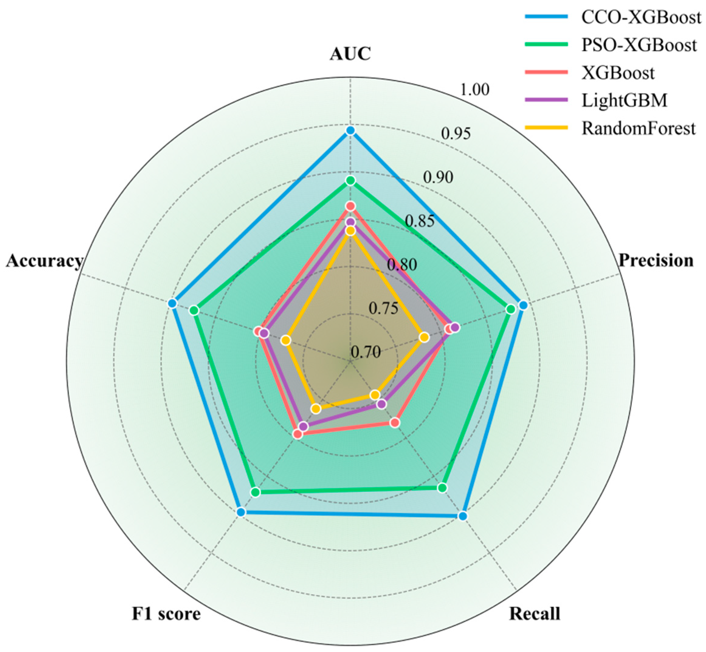
Based on the radar chart in Figure 5, the CCO-optimized XGBoost model is significantly better than other baseline models on key evaluation metrics. Compared with unoptimized XGBoost, LightGBM, RandomForest, and PSO-XGBoost models, this model achieves higher performance in accuracy, precision, recall, F1 value, and AUC. Moreover, all performance evaluation metrics of CCO-XGBoost exceed 0.85, and this result indicates a substantive improvement in model prediction ability by the CCO optimization strategy.

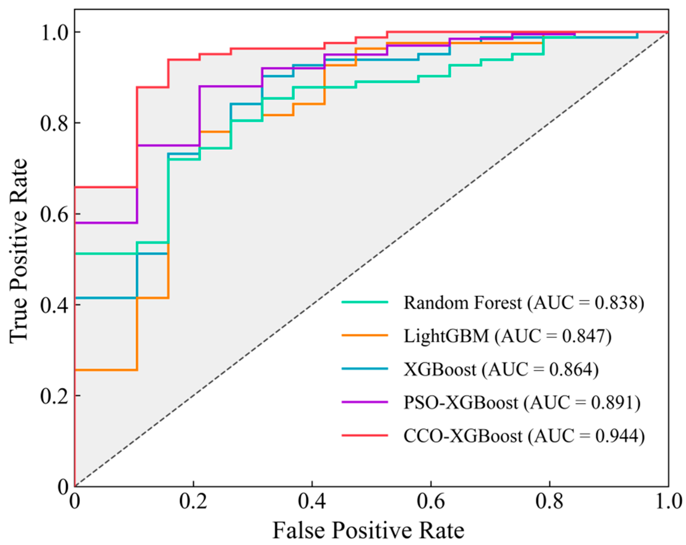
The ROC curves of the four models in Figure 6 and their corresponding AUC values are: RandomForest (0.838), LightGBM (0.847), XGBoost (0.864), PSO-XGBoost (0.891), and CCO-XGBoost (0.944). The ROC curve of the CCO-XGBoost model is closest to the upper-left corner, indicating that its performance was significantly improved after hyperparameter optimization.

The evaluation metrics of all models are summarized in

Table 2. Summary of model evaluation metrics.

Model	Precision	Accuracy	Recall	F1 Score	AUC
LightGBM	0.816	0.796	0.756	0.785	0.847
RandomForest	0.782	0.772	0.744	0.762	0.838
XGBoost	0.810	0.802	0.780	0.795	0.864
PSO-XGBoost	0.878	0.874	0.865	0.871	0.891
CCO-XGBoost	0.892	0.898	0.902	0.897	0.944

. The CCO-optimized XGBoost model is significantly better than all baseline models, confirming the effectiveness of the hyperparameter optimization strategy. Compared with the unoptimized XGBoost model, both precision and accuracy are significantly improved; the recall is increased by about 12.2% and the F1 score is increased by about 10.2%. Compared with the PSO-XGBoost model commonly used in geotechnical engineering, the recall is increased by about 3.7% and the F1 score is increased by about 2.6%, showing similarly significant advantages. The significant improvement in each metric further verifies that the CCO algorithm effectively alleviates problems such as class imbalance through dynamic parameter adjustment. In particular, the optimized model has an AUC of 0.944, which is about 8.0% higher than the unoptimized XGBoost model and about 5.3% higher than the PSO-XGBoost model. The model achieves the best overall performance in terms of accuracy (0.898), precision (0.892), recall (0.902), and F1 score (0.897). This performance advantage stems from the unique mechanism of the CCO algorithm, which effectively overcomes some defects of traditional algorithms and fundamentally improves the hyperparameter optimization accuracy and model robustness of XGBoost.

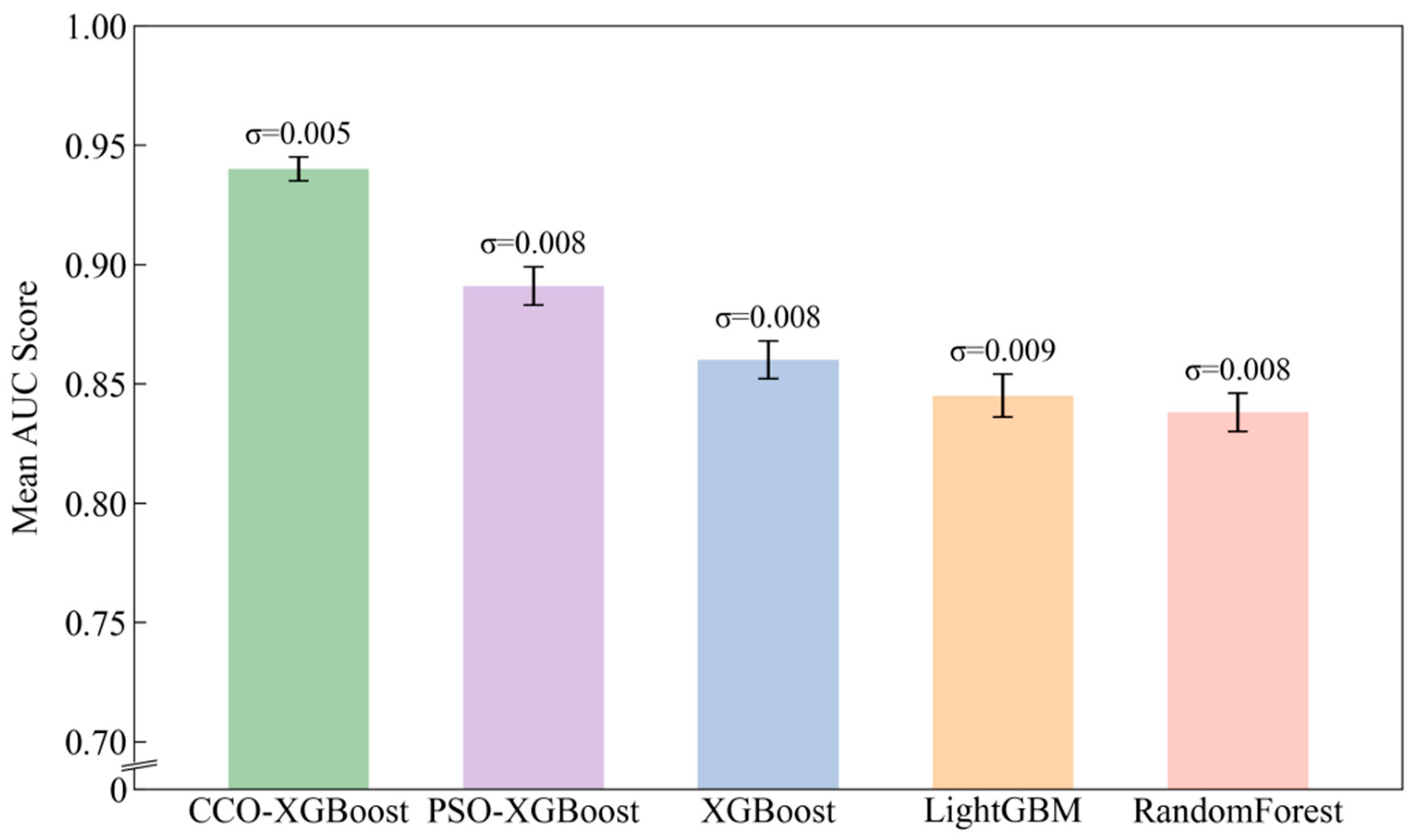
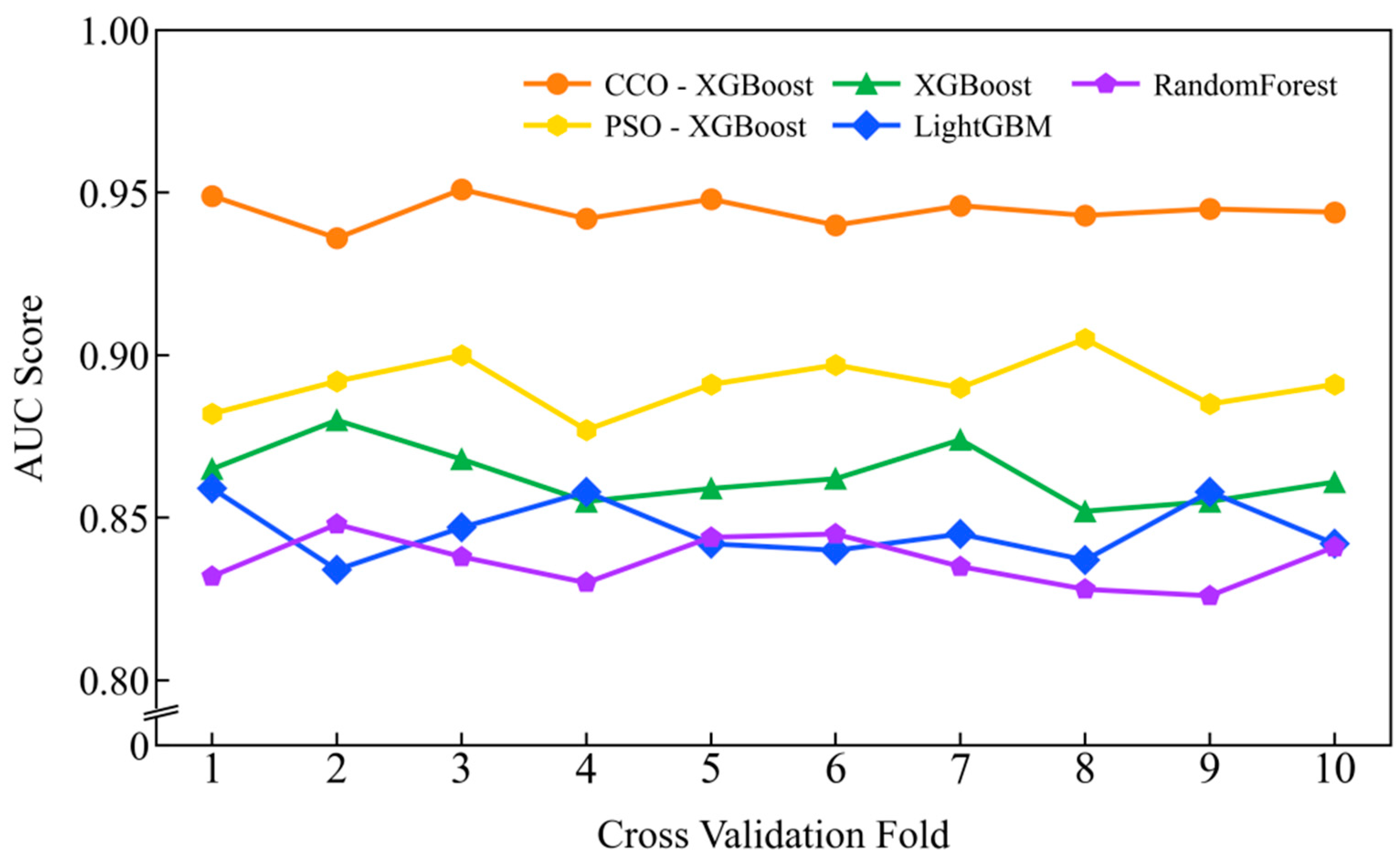
Ten-fold cross-validation is performed on the training set to implement the entire workflow of model training and CCO hyperparameter optimization. The training set samples are divided into 10 subsets by random stratified sampling. In each round, nine subsets are selected for training and parameter optimization, and one subset is used for internal validation. Repeated random partitioning effectively avoids the contingency arising from a single random sampling split. Based on the 10-fold cross-validation within the training set, the mean and standard deviation of AUC, the core evaluation indicator for imbalanced binary classification data, are calculated to quantify model stability and derive the corresponding confidence interval. As shown in Figure 7, the 10-fold comparison results indicate that the AUC values of CCO-XGBoost are consistently higher than those of other comparative models, with statistically significant performance improvement and little impact from random fluctuations. A t-test analysis of the 10-fold cross-validation results of CCO-XGBoost and PSO-XGBoost demonstrates that the performance difference between the two models is highly statistically significant (p < 0.001), revealing that the performance improvement achieved by the CCO algorithm originates from the optimization of its search mechanism rather than accidental bias caused by random fluctuations. The 10-fold cross-validation randomly divides samples involving different regions, lithology and hydrological conditions, which can effectively verify the generalization and adaptation ability of the model under various geotechnical working conditions and avoid overfitting under a single working condition.

As shown in Figure 8, the standard deviations of cross-validation results for each model are: XGBoost (0.008), LightGBM (0.009), RandomForest (0.009), PSO-XGBoost (0.008), and CCO-XGBoost (0.005). CCO-XGBoost has the lowest standard deviation (0.005), with highly concentrated numerical distribution and compact confidence interval. Slope stability prediction is susceptible to measured parameter deviations and dataset discreteness, which tends to induce fluctuations in prediction results. In contrast, the CCO-XGBoost model presents lower prediction dispersion and stronger robustness, effectively attenuating the interference of such factors on prediction outcomes and maintaining stable prediction performance even when engineering measured data contains deviations.

4.3. SHAP Analysis

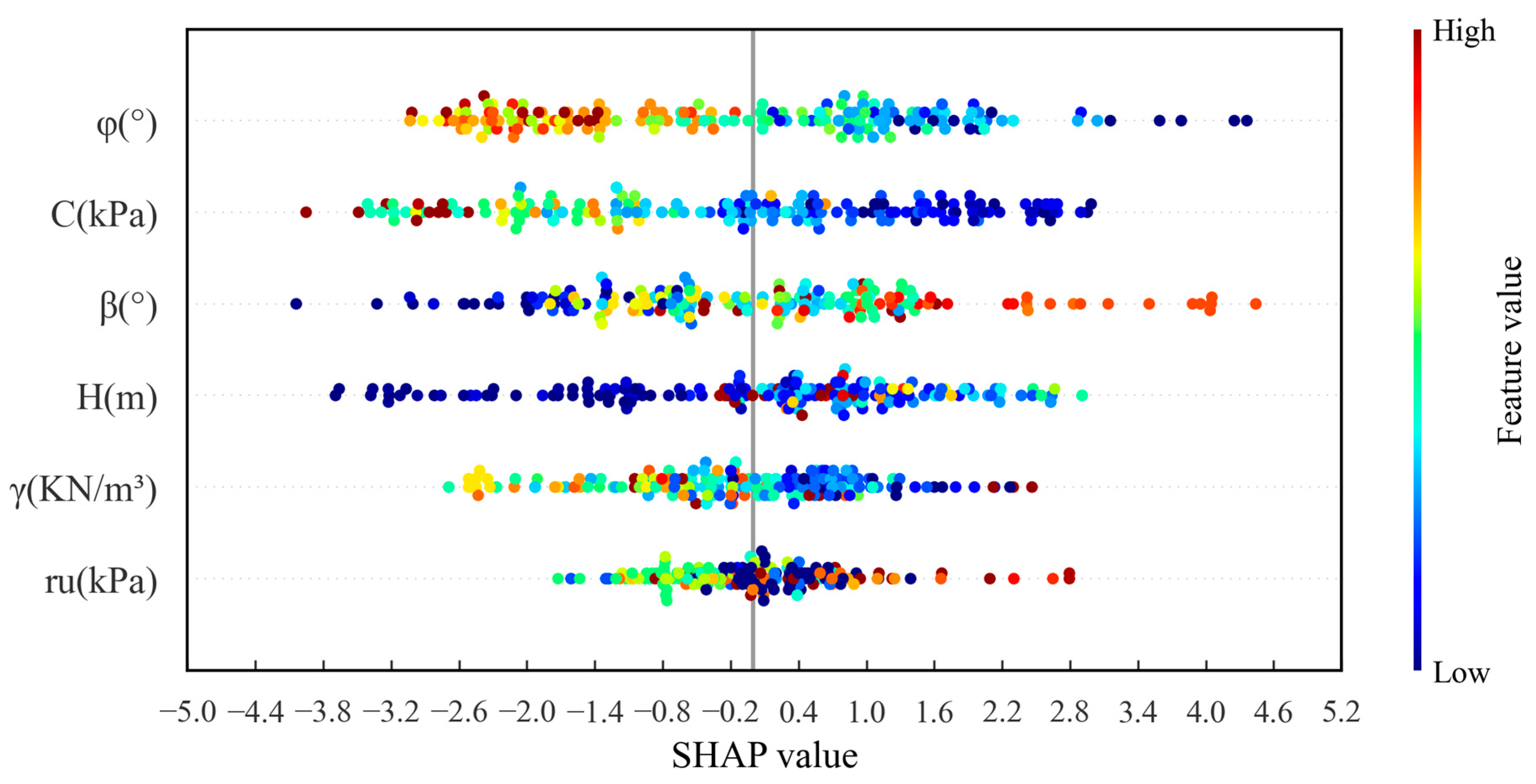
SHAP analysis is based on the Shapley value concept in game theory. Without changing the model structure, it can make the prediction results of the complex nonlinear XGBoost model interpretable [28]. Figure 9 reveals the global importance and marginal contribution of each feature to the predicted probability of slope instability, with the internal friction angle (φ) and cohesion (C) ranking in the top two. From a geomechanical perspective, the internal friction angle reflects the slipping and interlocking characteristics of rock and soil masses; lithological differences lead to differentiation of frictional properties, and its variation alters slope stress distribution by regulating frictional effects, thereby affecting the stability state of rock and soil masses [29]. Cohesion characterizes the interparticle bonding force of rock and soil masses, serving as a key mechanical indicator. Its attenuation significantly reduces the shear strength of rock and soil masses, deteriorates mechanical responses, and acts as a critical factor controlling slope failure [30]. Their dominant contributions essentially reflect the objective manifestation of the core mechanical mechanism of slopes, verifying the physical rationality of the model, with high φ and high C mostly corresponding to negative SHAP values, significantly reducing the instability probability and conforming to the Mohr–Coulomb failure criterion.

In terms of other feature values, the geometric parameters slope angle (β) and slope height (H) overall show unfavorable contributions. Many high-β points lie at positive SHAP values with a longer positive tail, indicating that increasing slope angle significantly raises instability risk; H shows “low H tends negative, high H tends positive,” indicating that an increase in slope scale enhances driving forces through self-weight and potential sliding mass effects. The influence of unit weight (γ) is relatively weak, but as its value increases, it shifts toward positive SHAP values overall, reflecting that higher unit weight is unfavorable to stability. Although pore water pressure ratio (r_u) ranks lower, high r_u corresponds to markedly positive SHAP values, indicating that under certain conditions, seepage can significantly amplify instability probability; the mechanism is that increased pore pressure reduces effective stress and weakens shear strength. The analysis results are consistent with traditional geotechnical mechanics understanding: φ and C play the dominant stabilizing role, while β, H, γ, and r_u mainly increase instability risk by increasing driving forces or reducing effective stress. In engineering, priority should be given to improving φ and C, controlling slope angle and slope height in coordination, and reducing the unfavorable influence of pore pressure ratio (r_u) to reduce the probability of instability. Overall, the SHAP sensitivity analysis shows that the model effectively characterizes nonlinear interactions among known geomechanical features.

The SHAP analysis results not only verify that the model predictions conform to classical mechanical properties and traditional geotechnical mechanics knowledge but also provide detailed insights that are difficult to quantitatively obtain using traditional slope analysis methods. This method quantifies the marginal contribution and nonlinear action law of each parameter, reveals the nonlinear interaction characteristics of multi-factor coupling, makes up for the deficiencies of traditional methods in single-factor analysis and linear assumptions, and can provide quantitative decision support for engineering parameter optimization and risk prevention and control that is difficult to be efficiently provided by traditional methods.

5. Engineering Case Verification

To further verify the performance and generalization ability of the CCO-XGBoost model, in addition to the 832 multi-source slope datasets, 12 real engineering cases [31,32] with distinct differences in regional conditions, geological conditions, lithology and slope type are selected for independent external validation. All these cases have no overlap with the original dataset and are not involved in model training and parameter optimization, which can effectively avoid data leakage and provide a more rigorous test for the model. The prediction results of engineering cases are shown in

Table 3. Verification results of engineering examples.

No.	H/(m)	Β/(°)	γ/(KN/m3)	C/(kPa)	φ/(°)	ru/(kPa)	Actual Status	Predicted Results
1	443.00	47.00	25.00	46.00	35.00	0.29	Stable	Stable
2	60.00	28.00	21.96	34.77	14.15	0	Stable	Stable
3	51.60	40.00	17.80	22.20	6.05	1.00	Unstable	Unstable
4	36.00	30.00	20.45	16.00	15.00	0.25	Stable	Stable
5	301.00	42.60	27.00	32.00	33.00	0.29	Unstable	Unstable
6	225.00	45.00	20.00	25.00	36.00	0.50	Unstable	Unstable
7	123.60	41.5	21.50	15.00	29.00	0.36	Stable	Stable
8	30.00	45.00	22.00	20.00	36.00	0.29	Unstable	Unstable
9	50.00	20.32	18.82	25.00	14.60	0.40	Unstable	Unstable
10	30.00	30.00	21.00	10.00	30.34	0.29	Stable	Stable
11	10.00	30.00	22.00	10.00	35.00	0.29	Stable	Stable
12	200.50	49.00	31.30	68.00	37.00	0.29	Unstable	Unstable

.

The model’s predictions for the 12 engineering cases are fully consistent with the actual field conditions, with all classification outputs showing high predictive confidence. These cases cover multiple critical working conditions, where relevant parameters fall within the critical interval between slope stability and instability, posing high classification difficulty. The model achieves accurate discrimination in all cases, which further indicates that the model has certain adaptability to such engineering cases.

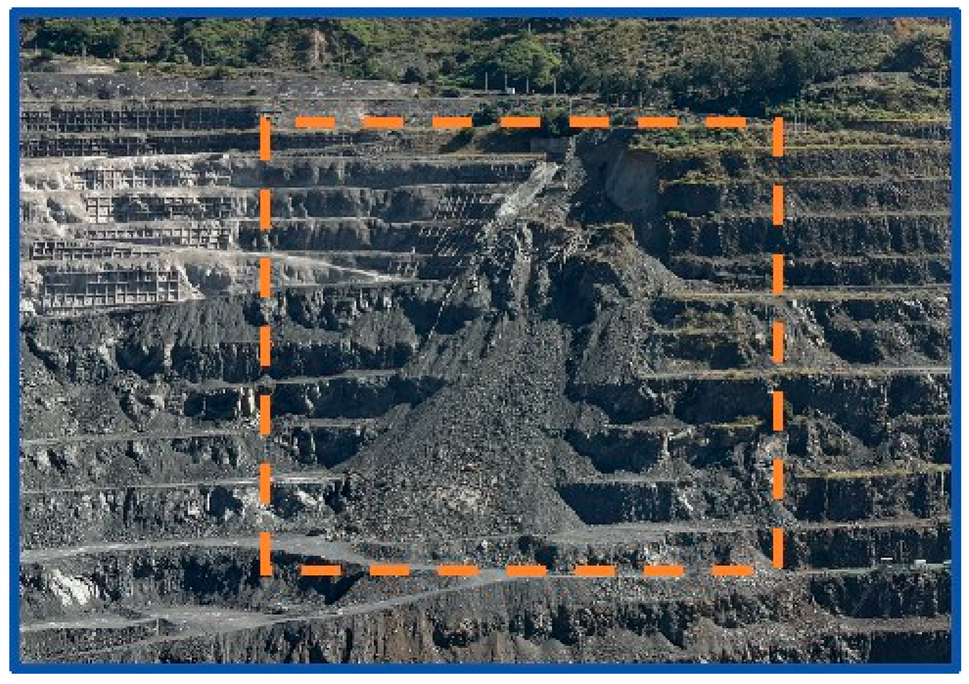
On the basis of overall verification, typical instability Case 6 is selected for analysis. The slope geometry and hydrological conditions are relatively unfavorable. The slope failure situation is shown in Figure 10: local collapse and sliding occurred and formed an accumulation body, indicating that under high and steep slope morphology conditions, relatively high pore water pressure led to reduced effective stress and weakened the shear strength of the potential shear zone, thereby causing continuous attenuation of local anti-sliding resistance and inducing instability expansion. Combined with SHAP interpretation: φ and C provide dominant stabilizing contributions to stability, while larger β, H, and high r_u significantly drive the instability probability positively. The model can accurately identify the combination of feature parameters and effectively characterize the nonlinear coupling and interaction effects of high, steep, and high-pore-pressure parameters in this engineering case. The discrimination result given for this case is consistent with the actual working conditions, reflecting the model’s generalization and classification reliability on real engineering samples.

These prediction results indicate that the model performs well in parameter optimization and feature correlation identification and has a strong ability to identify nonlinear interactions. Based on dataset training with multi-regional and multi-lithology conditions as well as independent external validation, the results show that the CCO-XGBoost model has good prediction adaptability to slopes under different geological and hydrological conditions. It can provide a reliable reference basis for the stability prediction of similar slope engineering.

6. Conclusions

This paper constructed a slope stability prediction model based on CCO-XGBoost, aiming to improve the efficiency and accuracy of slope stability evaluation and solve problems such as poor adaptability of traditional mechanical analysis methods under complex working conditions and challenges in multi-source data fusion. This model combines the global optimization ability of the CCO with the gradient boosting ensemble framework of XGBoost, performing adaptive adjustment of high-dimensional hyperparameters, and characterizing nonlinear interaction relationships between input features and stability responses through ensemble learning. The main conclusions of the study are as follows:

(1) A dataset containing 832 samples was constructed using six key parameters: slope height (H), slope angle (β), unit weight (γ), cohesion (C), internal friction angle (φ), and pore pressure ratio (r_u). The samples cover multiple regions, various lithology and different hydrogeological conditions, covering major influencing dimensions such as geometric conditions, material strength and seepage effects. Pearson correlation testing shows that this feature combination has good independence and can serve as a reasonable input feature system for model training.

(2) The optimized CCO-XGBoost model achieved relatively good comprehensive classification performance on the test set. The optimized model evaluation indicators are: AUC = 0.944, Accuracy = 0.892, Precision = 0.887, Recall = 0.874, and F1 score = 0.897. It achieved the best overall performance in all aspects, outperforming unoptimized XGBoost and baseline models such as LightGBM and RandomForest, as well as the widely used engineering optimization model PSO-XGBoost. This indicates that compared with traditional optimization algorithms, the CCO algorithm has formed substantial improvements in optimization-seeking mechanisms and implementation methods. It can effectively make up for some shortcomings of such algorithms, improve the model’s ability to distinguish samples, and enhance the reliability of discrimination results.

(3) The 10-fold cross-validation results show that model performance fluctuates little, reflecting that this method is not greatly affected by the division of training and validation sets. Under conditions where engineering data contain sample heterogeneity and noise disturbances, it can still maintain relatively stable prediction output, demonstrating good robustness. SHAP interpretation results show that φ and C have the greatest influence on instability probability, while β, H, γ, and higher r_u tend to increase instability risk. These patterns are consistent with the Mohr–Coulomb failure criterion and classic mechanical understanding of slope stability, and this analysis quantitatively clarifies the contribution degree and nonlinear coupling characteristics of each parameter from the data level, and provides quantitative new insights that are difficult to obtain efficiently by traditional analysis methods, forming an evidence chain of “high-precision prediction–interpretable mechanism–engineering implications.”

(4) Verification results based on actual slope engineering examples show that the model prediction results highly match the actual slope stability status. This fully verifies the model’s practicality and adaptability under complex nonlinear conditions, which can provide references for stability prediction and design of similar slope engineering.

(5) The current model is still limited by the dataset and the scale of actual engineering case samples, and analysis of complex hydrogeological structures and multi-source monitoring information is still relatively limited. Meanwhile, deep coupling with real-time monitoring systems and automated data workflows has not yet been formed. Follow-up research can further improve the model’s ability to perform reliable analysis in new scenarios by expanding cross-regional and cross-type samples and introducing information such as terrain and geology, rainfall infiltration, and monitoring sequences, combined with uncertainty quantification and probability calibration and other aspects. In the future, the model can be embedded with sensors to form an integrated platform framework with a real-time monitoring system, realizing continuous and large-scale slope stability prediction, and further improving robustness and early-warning application value in real engineering scenarios. Relevant verification scenarios can be expanded in practical applications to improve the engineering adaptability of the model.

References

- Shabbir, W.; Omer, T.; Pilz, J. The impact of environmental change on landslides, fatal landslides, and their triggers in Pakistan (2003–2019). Environ. Sci. Pollut. Res. 2023, 30, 33819–33832. [Google Scholar] [CrossRef] [Scilit] [PubMed]
- An, H.M.; Fan, Y.Q.; Liu, H.Y.; Cheng, Y.Y.; Song, Y.S. The State of the Art and New Insight into Combined Finite-Discrete Element Modelling of the Entire Rock Slope Failure Process. Sustainability 2022, 14, 4896. [Google Scholar] [CrossRef] [Scilit]
- Rajan, K.C.; Aryal, M.; Sharma, K.; Bhandary, N.P.; Pokhrel, R.; Acharya, I.P. Development of a framework for the prediction of slope stability using machine learning paradigms. Nat. Hazards 2025, 121, 83–107. [Google Scholar] [CrossRef] [Scilit]
- Zhang, J.; Liu, Z.; Zhang, S.; Guo, T.; Yuan, C. Slope Stability Prediction Based on WOA-RF Hybrid Model. Chin. J. High Press. Phys. 2024, 38, 194–205. Available online: https://link.cnki.net/urlid/51.1147.O4.20240129.1155.008 (accessed on 19 November 2025).
- Kurnaz, T.F.; Erden, C.; Dağdeviren, U.; Demir, A.S.; Kökçam, A.H. Comparison of machine learning algorithms for slope stability prediction using an automated machine learning approach. Nat. Hazards 2024, 120, 6991–7014. [Google Scholar] [CrossRef] [Scilit]
- Zhang, W.; Li, H.; Han, L.; Chen, L.; Wang, L. Slope stability prediction using ensemble learning techniques: A case study in Yunyang County, Chongqing, China. J. Rock Mech. Geotech. Eng. 2022, 14, 1089–1099. [Google Scholar] [CrossRef] [Scilit]
- Lin, S.; Zheng, H.; Han, B.; Li, Y.; Han, C.; Li, W. Comparative performance of eight ensemble learning approaches for the development of models of slope stability prediction. Acta Geotech. 2022, 17, 1477–1502. [Google Scholar] [CrossRef] [Scilit]
- Alharbi, H.S. Interpretable and Calibrated XGBoost Framework for Risk-Informed Probabilistic Prediction of Slope Stability. Sustainability 2025, 17, 10122. [Google Scholar] [CrossRef] [Scilit]
- Abbas, F.; Zhang, F.; Ismail, M.; Khan, G.; Iqbal, J.; Alrefaei, A.F.; Albeshr, M.F. Optimizing Machine Learning Algorithms for Landslide Susceptibility Mapping Along the Karakoram Highway, Gilgit Baltistan, Pakistan: A Comparative Study of Baseline, Bayesian, and Metaheuristic Hyperparameter Optimization Techniques. Sensors 2023, 23, 6843. [Google Scholar] [CrossRef] [Scilit]
- Ye, C.Z.; Wu, H.; Oguchi, T.; Tang, Y.T.; Pei, X.J.; Wu, Y.F. Physically Based and Data-Driven Models for Landslide Susceptibility Assessment: Principles, Applications, and Challenges. Remote Sens. 2025, 17, 2280. [Google Scholar] [CrossRef] [Scilit]
- Tang, X.; Chen, C.; Shan, D.; Zhang, P.; Xue, J. Slope reliability assessment using an innovative critical failure path approach. Front. Earth Sci. 2024, 12, 1428309. [Google Scholar] [CrossRef] [Scilit]
- Lin, H.; Li, L.; Qiang, Y.; Zhang, Y.; Liang, S.; Xu, X.; Li, H.; Hu, S. Sensitivity analysis of slope stability based on eXtreme gradient boosting and SHapley Additive exPlanations: An exploratory study. Heliyon 2024, 10, e35871. [Google Scholar] [CrossRef] [Scilit]
- Zhou, J.; Li, E.; Yang, S.; Wang, M.; Shi, X.; Yao, S.; Mitri, H.S. Slope stability prediction for circular mode failure using gradient boosting machine approach based on an updated database of case histories. Saf. Sci. 2019, 118, 505–518. [Google Scholar] [CrossRef] [Scilit]
- Kardani, N.; Zhou, A.; Nazem, M.; Shen, S. Improved prediction of slope stability using a hybrid stacking ensemble method based on finite element analysis and field data. J. Rock Mech. Geotech. Eng. 2021, 13, 188–201. [Google Scholar] [CrossRef] [Scilit]
- Ma, J.; Jiang, S.; Liu, Z.; Ren, Z.; Lei, D.; Tan, C.; Guo, H. Machine Learning Models for Slope Stability Classification of Circular Mode Failure: An Updated Database and Automated Machine Learning (AutoML) Approach. Sensors 2022, 22, 9166. [Google Scholar] [CrossRef] [Scilit]
- Hu, S.; Li, Y.; Shan, C.; Xue, X.; Yang, H. Research on Slope Stability Based on Improved PSO-BP Neural Network. J. Disaster Prev. Mitig. Eng. 2023, 43, 854–861. [Google Scholar] [CrossRef]
- Selamat, S.N.; Majid, N.A.; Taha, M.R. Multicollinearity and spatial correlation analysis of landslide conditioning factors in Langat River Basin, Selangor. Nat. Hazards 2025, 121, 2665–2684. [Google Scholar] [CrossRef] [Scilit]
- Chen, T.; Guestrin, C. In XGBoost: A Scalable Tree Boosting System. In Proceedings of the 22nd ACM SIGKDD International Conference on Knowledge Discovery and Data Mining, San Francisco, CA, USA, 2016; Association for Computing Machinery: San Francisco, CA, USA, 2016; pp. 785–794. [Google Scholar] [CrossRef] [Scilit]
- Wang, L.; Wu, C.; Tang, L.; Zhang, W.; Lacasse, S.; Liu, H.; Gao, L. Efficient reliability analysis of earth dam slope stability using extreme gradient boosting method. Acta Geotech. 2020, 15, 3135–3150. [Google Scholar] [CrossRef] [Scilit]
- Wang, T.; Gu, S.; Liu, R.; Chen, L.; Wang, Z.; Zeng, Z. Cuckoo catfish optimizer: A new meta-heuristic optimization algorithm. Artif. Intell. Rev. 2025, 58, 326. [Google Scholar] [CrossRef] [Scilit]
- Bharti, J.P.; Mishra, P.; Moorthy, U.; Sathishkumar, V.E.; Cho, Y.; Samui, P. Slope Stability Analysis Using Rf, Gbm, Cart, Bt and Xgboost. Geotech. Geol. Eng. 2021, 39, 3741–3752. [Google Scholar] [CrossRef] [Scilit]
- Lyu, J.; Hu, T.; Liu, G.; Cao, B.; Wang, W.; Li, S. Stability evaluation of open-pit mine slope based on Bayesian optimization 1D-CNN. Sci. Rep. 2024, 14, 13995. [Google Scholar] [CrossRef] [Scilit]
- Wang, L.; Zhang, C.; Wang, W.; Deng, T.; Ma, T.; Shuai, P. Slope Stability Assessment Using an Optuna-TPE-Optimized CatBoost Model. Eng 2025, 6, 185. [Google Scholar] [CrossRef] [Scilit]
- Hanandeh, S. Evaluation Circular Failure of Soil Slopes Using Classification and Predictive Gene Expression Programming Schemes. Front. Built Environ. 2022, 8, 858020. [Google Scholar] [CrossRef] [Scilit]
- Kong, T.; Shao, G.Y.; Shao, G.B.; Chen, L.L.; Liu, G.H. Slope Stability Prediction Utilizing a Random Forest Model Optimized by Particle Swarm Optimization. Geofluids 2025, 2025, 5088405. [Google Scholar] [CrossRef] [Scilit]
- Zerouali, B.; Bailek, N.; Tariq, A.; Kuriqi, A.; Guermoui, M.; Alharbi, A.H.; Khafaga, D.S.; El-kenawy, E.M. Enhancing deep learning-based slope stability classification using a novel metaheuristic optimization algorithm for feature selection. Sci. Rep. 2024, 14, 21812. [Google Scholar] [CrossRef] [Scilit]
- Lin, Y.; Zhou, K.; Li, J. Prediction of Slope Stability Using Four Supervised Learning Methods. IEEE Access 2018, 6, 31169–31179. [Google Scholar] [CrossRef] [Scilit]
- Gao, W.; Zang, M.; Mei, G. Exploring influence of groundwater and lithology on data-driven stability prediction of soil slopes using explainable machine learning: A case study. Bull. Eng. Geol. Environ. 2023, 83, 2. [Google Scholar] [CrossRef] [Scilit]
- Talukdar, M.; Sone, H.; Kuo, L. Lithology and Fault-Related Stress Variations Along the TCDP Boreholes: The Stress State Before and After the 1999 Chi-Chi Earthquake. J. Geophys. Res. Solid Earth 2022, 127, e2021JB023290. [Google Scholar] [CrossRef] [Scilit]
- Wang, D.; Ma, W.; Niu, Y.; Chang, X.; Wen, Z. Effects of cyclic freezing and thawing on mechanical properties of Qinghai–Tibet clay. Cold Reg. Sci. Technol. 2007, 48, 34–43. [Google Scholar] [CrossRef] [Scilit]
- Shu, T.; Tao, W.; Lu, H.T.; Li, H.; Cao, J.X.; Ma, J.W. A Hybrid Random Forest and Least Squares Support Vector Machine Model Based on Particle Swarm Optimization Algorithm for Slope Stability Prediction: A Case Study in Sichuan-Tibet Highway, China. Adv. Civ. Eng. 2023, 2023, 6651323. [Google Scholar] [CrossRef] [Scilit]
- Wang, T.; Wang, C.; Wu, S.; Wang, Q.; Xu, J. Slope stability prediction and application based on MISSA-SVM model. China Saf. Sci. J. 2024, 34, 135–144. [Google Scholar] [CrossRef]