Risk-Aware Predictive–Proactive Sustainable Scheduling for Dynamic Flexible Job Shops Under Carbon and Labor Uncertainty

Abstract

Dynamic flexible job shop scheduling (DFJSP) faces compound uncertainty from job arrivals, machine breakdowns, labor volatility, and fluctuating carbon signals, and reactive or expectation-based methods cannot prevent costly tail events. This study proposes a five-stage risk-aware predictive–proactive framework that combines rolling-horizon forecasting, Conditional Value at Risk (CVaR) assessment, proactive pre-allocation of time buffers, preventive maintenance, and energy flexibility, risk-adaptive MOEA/D, and real-time control by a graph-attention reinforcement learning (RL) agent. MOEA/D and the agent exchange knowledge bidirectionally: RL trajectories seed the evolutionary search, and non-dominated solutions regularize policy learning. Over 30 independent runs under high compound uncertainty, the framework reduces delay CVaR by 65.4%, carbon emissions by 24.5%, and labor-shortage CVaR by 65.4% relative to NSGA-II, and by 49.3%, 9.8%, and 49.3% relative to single-agent deep RL, the strongest baseline, while keeping online decision latency below one second at the largest scale tested.

1. Introduction

Modern smart factories operate under persistent, coupled uncertainty rather than isolated disturbances [1,2,3]. Scheduling decisions are simultaneously affected by stochastic order arrivals [3,4], machine degradation and failure [5,6], labor-availability fluctuations [7], time-of-use electricity pricing [8], and dynamic carbon-intensity signals [9,10]. The flexible job shop scheduling problem (FJSP), in which each operation may be processed by several alternative machines, is a well-established NP-hard problem [1,11]; under these uncertainties, it evolves into the dynamic FJSP (DFJSP), where preplanned schedules must be repeatedly revised [2,3,4,6,12], and static or purely reactive policies lose validity [2,13]. Heuristic, metaheuristic, and rolling-rescheduling approaches [2,12,13] mostly optimize average performance and therefore remain vulnerable when extreme events dominate system loss [11,12,13,14].

This limitation is particularly serious in sustainable manufacturing [8,9,10,15,16,17]. Under time-varying electricity prices [8], peak-load restrictions [16], and carbon-emission constraints [9,10,18,19], a schedule that performs well in expectation may still cause severe power peaks, costly emergency labor reallocations, or unstable rescheduling cascades when uncertainty unfolds unfavorably [7,16,20]. Modern scheduling systems must therefore be risk-aware, proactive, and robust to tail events, in addition to being efficient [14,20,21,22].

Two method families address parts of this problem. Deep reinforcement learning (DRL) has improved real-time dispatching [3,4,5,6,12,19,23,24], and graph neural networks [23,24], graph-attention networks [25], and attention/ranking mechanisms [5] strengthen state representation, but RL-oriented scheduling is often short-horizon and reward-driven, which leads to myopic decisions when global multi-objective trade-offs are not explicitly controlled [26,27,28,29]. Multi-objective evolutionary algorithms such as NSGA-II [28], SPEA2 [27,28,29], and MOEA/D [13,24,25] balance efficiency, energy, carbon, and stability objectives globally [9,15,17,30]; MOEA/D is particularly suitable because its decomposition strategy improves convergence and diversity [15,26,27], but standalone evolutionary search is too slow for high-frequency online updates [2,3,24]. Existing hybrid RL–evolutionary approaches follow a loosely coupled or sequential architecture in which the learning model at most initializes the evolutionary population and receives no continuous structured feedback [3,12,15,26,27], and they rarely integrate uncertainty forecasting, risk quantification [14,21], proactive buffer allocation, and risk-adaptive decomposition in one framework [20,22,27].

To address this gap, this study reformulates the problem as a risk-aware predictive–proactive sustainable scheduling task under compound uncertainty [1,2,7,8,14] and integrates forecasting, tail-risk control [14,21], proactive intervention [20], multi-objective search [15,27], and event-driven execution [3,6,24] into a single five-stage architecture (Section 3). DFJSP remains the core scientific object: sustainability, human-centric fairness, and schedule stability enter as risk-aware extensions of the DFJSP objective, and every contribution is evaluated by its effect on DFJSP decision quality under compound uncertainty rather than as a general smart-factory risk-control framework.

The major contributions of this study are summarized as follows:

• A predictive uncertainty layer estimates machine-failure probability [5,6], order-arrival intensity [3,4], labor availability [7], and energy–carbon signals [8,10,16] over a rolling horizon, and a CVaR-embedded multi-objective formulation [14,21] covers efficiency, sustainability [9,10,17], human-centric cost [7], and schedule stability [20].
• A proactive decision layer allocates time buffers, preventive maintenance, and energy-flexibility reserves before disruptions materialize [20].
• A bidirectional risk-conditioned graph-attention RL–MOEA/D mechanism is designed, in which RL trajectories seed global search and MOEA/D non-dominated solutions [26,27,31] regularize policy learning; its contribution is isolated by unidirectional-coupling ablations (Section 4.6).
• An experimental protocol evaluates average values, Pareto quality [30,31,32], worst-case performance, variance, CVaR reduction [14,21], ablation contributions, and real-time feasibility using rigorous statistical testing [33].

The remainder of this paper is organized as follows. Section 2 reviews related work, Section 3 presents the proposed methodology, Section 4 introduces the experimental setup and evaluation metrics [31,32,33], Section 5 reports and discusses the results, and Section 6 concludes the study.

2. Literature Review

2.1. Flexible and Dynamic Job Shop Scheduling

The classical job shop scheduling problem [11] and its flexible variant (FJSP) [1,11,34] have long been recognized as representative NP-hard optimization problems [1,2]. Early research emphasized tabu search [1], dispatching heuristics [11], lot-sizing integration [34], and route-selection strategies [1], while later studies developed sophisticated multi-objective and hybrid optimization approaches to address machine flexibility and production complexity [2,28,29]. In the dynamic extension of FJSP (DFJSP), random job arrivals [3,4], machine breakdowns [5,6,12], and uncertain processing environments [6] make static schedules quickly obsolete [2].

Dynamic scheduling research has therefore focused on event-driven rescheduling, rolling-horizon optimization, and adaptive dispatching [2,3,12,13]. These methods improve responsiveness, yet many remain centered on average makespan or tardiness minimization and do not explicitly model the operational consequences of low-probability, high-impact events [14,20,21]. This gap becomes critical when sustainable production [8,9,10] and labor uncertainty [7] are simultaneously considered.

Critically, these studies typically validate their methods on stationary benchmark variants or single-disturbance scenarios and rarely quantify how performance degrades when several uncertainty sources materialize jointly. This study advances the state of the art by explicitly modeling four concurrent uncertainty processes—machine disruption, demand arrival, sustainability signals, and workforce availability—within a single rolling-horizon predictive layer, rather than treating each disturbance type in isolation.

2.2. Risk-Aware and Robust Scheduling

Robust scheduling and uncertain-environment optimization have highlighted the need to move beyond deterministic planning [20,22]. Existing resilient scheduling studies commonly incorporate uncertainty sets, scenario-based robustness, or recovery-oriented criteria to mitigate the effects of disruption [20]. However, robustness is often handled qualitatively or through worst-case approximations, which may be overly conservative or disconnected from probabilistic tail behavior [20,21,22].

Risk-aware metrics such as Value at Risk (VaR) and Conditional Value at Risk (CVaR) [20,21] offer a stronger basis for uncertainty-sensitive decision-making because they quantify not only the threshold of unfavorable outcomes but also the expected severity of extreme losses beyond that threshold [20,21]. Despite their relevance, explicit CVaR integration remains underdeveloped in dynamic flexible job shop scheduling [14,20,21], particularly in sustainable [9,10,13] and human-centric contexts [7]. This motivates the present study to embed CVaR directly into the multi-objective scheduling formulation [20,21,27].

Existing CVaR-based scheduling studies [14,20,21] are further limited in two respects: the risk term is typically attached to a single objective (e.g., cost or delay) rather than embedded across a multi-objective structure, and the risk-aversion parameter is fixed rather than adapted to the current operating condition. This study addresses both limitations by embedding CVaR into all four scheduling objectives simultaneously and by allowing the multi-objective decomposition weights to adapt to the online risk state (Section 3.5), a capability that prior CVaR-based scheduling studies do not provide.

2.3. Sustainable and Human-Centric Scheduling

Low-carbon and energy-aware scheduling has become a major theme in smart manufacturing due to net-zero targets and regulatory pressure [8,9,10,13,15,16,17,18,19]. Existing studies have investigated energy-aware machine assignment under time-of-use (TOU) electricity pricing [8], total carbon footprint minimization [9,18], peak shaving [16], space-cooperation energy reduction [17], and dynamic scheduling in low-carbon distributed systems [13,19]. These works demonstrate that energy and carbon objectives cannot be treated as secondary concerns because poor scheduling policies may increase both operational costs and environmental impact [8,9,10,16].

At the same time, emerging gig-based labor arrangements and Industry 5.0 concepts have elevated human-centric performance to a core scheduling concern [7]. Workload balance, labor utilization, fairness, and external labor cost now directly influence system resilience and long-term operational quality [7]. Yet sustainability [8,9,10] and workforce uncertainty [7] are still often modeled separately, rather than jointly under a unified dynamic risk framework [14,20].

A further limitation of this literature is that sustainability and workforce objectives are almost always optimized against expected values, so a schedule can appear efficient on average while still producing severe peak-load or labor-shortage episodes under adverse realizations. This study closes that gap by attaching CVaR-based tail-risk terms directly to the sustainability and human-centric objectives (Equations (4) and (5)), rather than treating them as deterministic or purely expectation-based costs as in prior work [7,8,9,10,13,15,16,17,18,19].

2.4. Reinforcement Learning for DFJSP

Deep reinforcement learning has shown strong potential in dynamic scheduling because it can learn adaptive dispatching policies through repeated interaction with the environment [3,4,5,6,12,13,19,23,24]. Recent studies have adopted actor–critic structures [3,6], multi-agent manufacturing architectures [12], graph neural network representations [23,24], and MachineRank/attention mechanisms [5] to improve scalability and topological understanding in DFJSP. These advances make RL especially attractive for event-driven decision-making at the shop-floor level [3,6,24].

However, RL methods usually optimize a scalar reward and can become biased toward immediate gains [3,6,19]. Without structured global guidance [26,27], learned policies may fail to maintain Pareto quality [30,31,32], long-horizon stability [20], or tail-risk control [14,21] across multiple competing objectives [15,28,29]. Therefore, RL should be integrated with a principled multi-objective optimizer [26,27] rather than used as a stand-alone scheduler.

Beyond the myopia concern noted above, existing RL-based DFJSP studies also provide little mechanism for injecting global multi-objective structure into the learned policy beyond reward shaping, and they rarely report Pareto-quality metrics (e.g., Hypervolume, IGD) that would allow direct comparison with evolutionary multi-objective baselines. This study addresses this gap through the bidirectional RL–MOEA/D coupling described in Section 3.5, which explicitly transfers Pareto-front structure into policy learning rather than relying on reward shaping alone.

2.5. Hybrid RL–MOEA/D Frameworks

Hybrid frameworks combine learning and evolutionary optimization to leverage the complementary strengths of local adaptation and global search [3,12,15,26,27]. MOEA/D [27] is especially attractive in this setting because its decomposition-based design scales well to multi-objective problems [15,26] and can exploit structural preference information [26,27]. Prior studies have shown that RL-assisted MOEA/D [15,26] and knowledge-guided decomposition methods [26,27] can improve optimization quality in uncertain or energy-aware scenarios [15,17].

Nevertheless, most existing hybrids are sequential rather than deeply co-adaptive [26,27]. They seldom incorporate predictive uncertainty modeling, risk-conditioned decision-making [20,21], or continuous bidirectional transfer between Pareto search and policy learning [26,27]. As a result, the literature still lacks an integrated framework that unifies prediction, CVaR-based risk assessment [14,21], proactive control [20], adaptive decomposition [26,27], and robust online scheduling [3,24] for sustainable DFJSP [7,9,10,15].

2.6. Research Gap Positioning

Table 1 summarizes how this study differs from representative prior work along five design dimensions that jointly define its contribution: uncertainty scope, risk treatment, RL–MOEA/D coupling direction, proactive control, and evaluation protocol. No single prior study combines joint multi-source uncertainty forecasting, multi-objective CVaR embedding, bidirectional RL–MOEA/D knowledge transfer, and proactive pre-disruption control within one framework; the ablation study in Section 5.4 further isolates the contribution of each of these components, providing empirical rather than purely descriptive support for their necessity.

Table 1. Positioning of this study relative to representative prior work along five key design dimensions.

Dimension	Representative Prior Work	This Study
Uncertainty scope	Single-source disruption or demand uncertainty [2,3,4,5,6,12,23]	Four concurrent sources (failure, arrival, carbon/energy, labor) with joint rolling-horizon forecasting
Risk treatment	Expectation-based objectives, or CVaR on a single objective [14,20,21]	CVaR embedded in all four multi-objective terms with risk-adaptive decomposition weighting
RL–MOEA/D coupling	Sequential, one-way coupling: RL seeds MOEA/D only [15,26,27]	Bidirectional coupling: RL trajectories seed MOEA/D and non-dominated solutions guide RL via policy distillation
Proactive control	Reactive rescheduling after disruption [2,12,13]	Proactive buffer, maintenance, and energy-flexibility allocation before disruption, guided by forecasts
Evaluation protocol	Mean objective values and a single Pareto front [28,29,30,31,32]	Worst-case, variance, CVaR, ablation, and real-time latency, validated with Friedman/Wilcoxon tests

3. Methodology

3.1. Problem Description and Uncertainty Modeling

This study considers a dynamic flexible job shop scheduling problem in a smart manufacturing environment with carbon and labor uncertainty. Let the job set be $\mathcal{J}=\{J_1,\dots ,J_n\}$ and the machine set be $\mathcal{M}=\{M_1,\dots ,M_m\}$. Each job $J_j$ consists of an ordered operation sequence $\{O_{j,1},\dots ,O_{j,K_j}\}$, where each operation can be processed by one machine from a feasible subset ${\mathcal{M}}_{j,k}\subseteq \mathcal{M}$. The decision variables include machine assignment $x_{j,k}^{\left(i\right)}\in \{0,1\}$ and operation start time $S_{j,k}^{\left(i\right)}$.

Unlike deterministic FJSP, the production environment evolves under stochastic and time-varying uncertainty. Four uncertainty sources are considered in this formulation:

• Machine disruption process represented by failure probability $P_{fail}^i\left(t\right)$.
• Dynamic demand process represented by order-arrival intensity $\lambda \left(t\right)$.
• Sustainability process represented by time-varying electricity and carbon signal $C_{grid}\left(t\right)$.
• Workforce process represented by labor-availability level $W\left(t\right)$.

To support proactive decision-making, the system employs a rolling-horizon prediction module that estimates future uncertainty trajectories over horizon $H$:

$${\stackrel{\mathbf{ˆ}}{\mathbf{u}}}_{t:t+H}={\mathsf{\Phi }}_{pred}\left({\mathbf{x}}_{0:t}\right)$$

(1)

where ${\mathbf{x}}_{0:t}$ denotes historical shop-floor observations and ${\stackrel{\mathbf{ˆ}}{\mathbf{u}}}_{t:t+H}$ contains predicted values of machine-failure probability, order-arrival intensity, labor availability, and energy–carbon states. The predictor can be implemented through a temporal-attention model, a Transformer-style forecaster, or a graph–temporal network that captures job–machine–resource coupling.

The prediction layer converts the scheduling problem from purely reactive rescheduling into anticipatory control. Instead of waiting for breakdowns or load spikes to occur, the scheduler estimates future risk exposure and prepares suitable buffers and operational adjustments in advance.

3.2. Risk-Aware Multi-Objective Formulation

The proposed framework optimizes four objectives covering efficiency, sustainability, human-centric cost fairness, and schedule stability. Each objective is formulated as an expectation-plus-tail-risk criterion so that both average performance and extreme-event severity are considered.

The multi-objective optimization problem is defined as:

$$\mathrm{m}\mathrm{i}\mathrm{n}F\left(\pi \right)=\left(f_1\right(\pi ),f_2(\pi ),f_3(\pi ),f_4(\pi \left)\right)$$

(2)

where $\pi$ denotes a scheduling policy or schedule plan.

The efficiency objective is defined as:

$$f_1=\mathbb{E}\left[C_{\mathrm{m}\mathrm{a}\mathrm{x}}\right]+{\gamma }_1{\mathrm{C}\mathrm{V}\mathrm{a}\mathrm{R}}_{\alpha }\left(C_{\mathrm{m}\mathrm{a}\mathrm{x}}\right)$$

(3)

where $C_{\mathrm{m}\mathrm{a}\mathrm{x}}$ is the makespan and ${\gamma }_1$ controls tail-risk sensitivity.

The sustainability objective jointly considers total energy, total carbon emission, and peak-load risk:

$$f_2=\mathbb{E}[E_{tot}+{\eta }_{1}C{O}_{2,tot}+{\eta }_{2}PER]+{\gamma }_2{\mathrm{C}\mathrm{V}\mathrm{a}\mathrm{R}}_{\alpha }\left(P_{max}\right)$$

(4)

where $E_{tot}$ is total energy consumption, $C{O}_{2,tot}$ is total carbon emission, $PER$ is the peak-energy ratio, and $P_{max}$ denotes peak-power demand.

The human-centric objective is formulated as:

$$f_3=\mathbb{E}[{\omega }_1{L}_{gig}+{\omega }_2{B}_{load}]+{\gamma }_3{\mathrm{C}\mathrm{V}\mathrm{a}\mathrm{R}}_{\alpha }\left(L_{short}\right)$$

(5)

where $L_{gig}$ is external labor cost, $B_{load}$ is workload imbalance, and $L_{short}$ is labor-shortage severity.

The schedule-stability objective is defined as:

$$f_4=\mathbb{E}[{\Delta }_{pro}+\rho {\Delta }_{rea}]+{\gamma }_4{\mathrm{C}\mathrm{V}\mathrm{a}\mathrm{R}}_{\alpha }(\Delta )$$

(6)

where ${\Delta }_{pro}$ denotes proactive adjustment magnitude, ${\Delta }_{rea}$ denotes reactive deviation after disruption realization, and $\Delta$ is the total schedule-change severity.

The CVaR term is defined as [18,19]:

$${\mathrm{C}\mathrm{V}\mathrm{a}\mathrm{R}}_{\alpha }(Z)=\underset{\zeta \in \mathbb{R}}{\mathrm{m}\mathrm{i}\mathrm{n}} \left\{\zeta +{\displaystyle \frac{1}{1-\alpha }}\mathbb{E}\left[\right(Z-\zeta {)}^{+}]\right\}$$

(7)

where $\alpha \in (0,1)$ is the confidence level and $(x{)}^{+}=\mathrm{m}\mathrm{a}\mathrm{x}(x,0)$. This formulation enables the framework to control the expected severity of extreme outcomes rather than only the average case.

3.3. Predictive–Proactive Framework Architecture

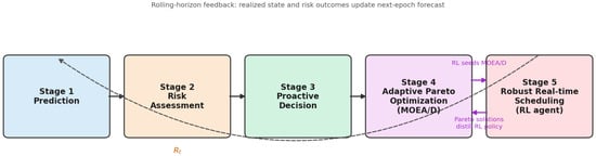
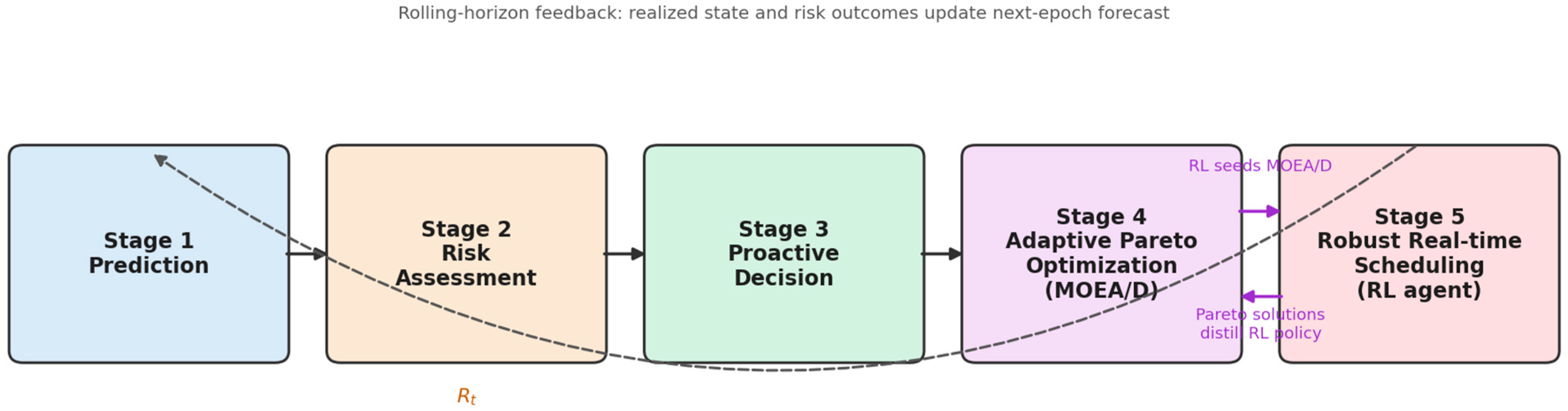
The overall scheduling architecture follows a five-stage decision flow as shown in Figure 1.

Figure 1. Five-stage architecture overview of the proposed risk-aware predictive–proactive framework. Dashed arrows indicate the rolling-horizon feedback loop; purple arrows indicate the bidirectional RL–MOEA/D knowledge transfer described in Section 3.5.

Stage 1: Prediction: Historical production data and current system observations are fed into the forecaster to estimate short-horizon trajectories of failure risk, order arrivals, energy–carbon signals, and workforce fluctuations.

Stage 2: Risk Assessment: The forecast outputs are converted into risk indicators such as delay risk, peak-energy risk, labor-shortage risk, and instability risk. The aggregated risk state is expressed as:

$$R_t=\psi ({\hat{P}}_{fail}(t:t+H),\hat{\lambda }(t:t+H),{\hat{C}}_{grid}(t:t+H),\hat{W}(t:t+H))$$

(8)

where $\psi (\cdot )$ maps forecast trajectories into risk features and tail-sensitive scores.

Concretely, $\psi (·)$ is implemented as four independently calibrated risk scores, one per uncertainty source $k\in \{\mathrm{f}\mathrm{a}\mathrm{i}\mathrm{l},\mathrm{a}\mathrm{r}\mathrm{r},\mathrm{e}\mathrm{n},\mathrm{l}\mathrm{a}\mathrm{b}\}$, each obtained by passing the corresponding predicted trajectory through a soft-plus tail transform:

$$r_k(t)=\mathrm{l}\mathrm{o}\mathrm{g}\left(1+\mathrm{e}\mathrm{x}\mathrm{p}\left({\displaystyle \frac{{\hat{\mu }}_k(t:t+H)-{\tau }_k}{{\sigma }_k}}\right)\right)$$

(9)

where ${\hat{\mu }}_k(t:t+H)$ is the predicted mean of source $k$ over the horizon, ${\tau }_k$ is a source-specific alarm threshold calibrated from the historical 90th percentile of source $k$, and ${\sigma }_k$ is the corresponding historical standard deviation. The four scores are concatenated into the risk-state vector $R_t=\left[r_{\mathrm{f}\mathrm{a}\mathrm{i}\mathrm{l}}\right(t),r_{\mathrm{a}\mathrm{r}\mathrm{r}}(t),r_{\mathrm{e}\mathrm{n}}(t),r_{\mathrm{l}\mathrm{a}\mathrm{b}}(t\left)\right]$, which is used both by the proactive decision layer (Stage 3) and by the weight-adaptation operator $\mathcal{A}(·)$ in Section 3.5 (Equation (19)).

Stage 3: Proactive Decision: Before disturbances occur, the scheduler allocates preventive actions based on risk severity, including time buffer allocation $b_{j,k}$, preventive maintenance activation $m_i$, and energy-flexibility reserve $e_t^{flex}$. These decisions reduce the need for severe reactive rescheduling later.

Stage 4: Adaptive Pareto Optimization: The multi-objective search is handled by MOEA/D, but the decomposition preference is adjusted according to the current risk profile so that high-risk periods emphasize stability, tail-risk containment, or energy-peak control more strongly.

Stage 5: Robust Real-time Scheduling: A risk-conditioned graph-attention RL agent (Section 3.4) executes event-driven micro-adjustments at runtime, including dispatching, machine reassignment, selective rescheduling, and energy-aware machine control.

This five-stage design differs from conventional reactive hybrids because proactive control is inserted between prediction and online execution. Consequently, the framework is not limited to responding after disruption but instead combines anticipation, protection, and adaptation in one decision loop.

3.4. Risk-Conditioned Graph-Attention RL Agent Design

The online scheduling component is modeled as a Markov Decision Process $(\mathcal{S},\mathcal{A},\mathcal{P},\mathcal{R})$. The state $s_t$ includes both current and predicted information:

$$s_t=[s_t^{shop},{\stackrel{\mathbf{ˆ}}{\mathbf{u}}}_{t:t+H},R_t]$$

(10)

where $s_t^{shop}$ contains machine states, operation queues, due-date slack, labor availability, machine loading, and energy/carbon context.

The action space extends beyond ordinary dispatching. At each decision epoch, the agent may choose job dispatching, machine assignment, preventive maintenance activation, dynamic voltage and frequency scaling, standby control, and localized rescheduling scope. This richer action space is necessary because sustainable scheduling under uncertainty depends not only on routing and sequencing but also on preventive and energy-flexible interventions.

The reward function is designed to discourage short-sighted policies and excessive risk-taking:

$$r_t=-({\beta }_1{C}_{inc}+{\beta }_2{E}_{inc}+{\beta }_{3}C{O}_{2,inc}+{\beta }_4{\Delta }_t+{\beta }_5{\mathcal{R}}_t)$$

(11)

where $C_{inc}$, $E_{inc}$, and $C{O}_{2,inc}$ are incremental efficiency and sustainability penalties, ${\Delta }_t$ is rescheduling deviation, and ${\mathcal{R}}_t$ is a risk penalty derived from predicted tail exposure or violation severity.

The DFJSP state is inherently relational and topology-dependent, which a flat vector cannot represent. The shop-floor part of the state, $s_t^{\mathrm{s}\mathrm{h}\mathrm{o}\mathrm{p}}$ in Equation (10), is therefore encoded by a graph-attention network (GAT) [34] that is trained jointly with the policy; this agent is hereafter called the risk-conditioned RL agent. The graph construction, the attention mechanism, and the coupling with the policy network are specified below.

Graph construction: At each decision epoch, the shop floor is represented as a heterogeneous directed graph $G_t=({\mathcal{V}}_t,{\mathcal{E}}_t)$ whose node set ${\mathcal{V}}_t={\mathcal{V}}_t^{\mathrm{o}\mathrm{p}}\cup {\mathcal{V}}_t^{\mathrm{m}\mathrm{c}}$ contains one operation node for every unfinished operation $O_{j,k}$ and one machine node for every machine $M_i$. An operation node is described by its minimum and maximum feasible processing times, the number of remaining operations of its job, its due-date slack, and a one-hot status (waiting, ready, or in process). A machine node is described by its current load, the remaining processing time of the operation in progress, its power state and energy rate, and its predicted failure probability $P_i^{\mathrm{f}\mathrm{a}\mathrm{i}\mathrm{l}}(t:t+H)$ taken from $u_{t:t+H}$. Three edge types are constructed: (i) precedence edges $O_{j,k}\to O_{j,k+1}$ within each job; (ii) alternative-routing edges, in both directions, between $O_{j,k}$ and every feasible machine $M_i\in M_{j,k}$, whose attribute ${\epsilon }_{vu}$ contains the processing time and energy consumption of that assignment; and (iii) resource-contention edges, in both directions, between each machine and the operations currently waiting in its queue or in process. The graph is rebuilt at every decision epoch, so that job arrivals, breakdowns, and completed operations are reflected immediately. The system-level forecasts $\lambda (t:t+H)$, $C^{\mathrm{g}\mathrm{r}\mathrm{i}\mathrm{d}}(t:t+H)$, and $W(t:t+H)$ and the risk-state vector $R_t$ are not attached to individual nodes but enter the policy at the graph level (Equation (16)).

Attention encoder: Each node first receives a type-specific linear projection of its features, $h_v^{\left(0\right)}={\Theta }_{\mathrm{t}\mathrm{y}\mathrm{p}\mathrm{e}\left(v\right)}{x}_v$. The encoder then stacks $L=3$ graph-attention layers with four attention heads each. In layer $l$ and head $\kappa$, the attention logit between a node $v$ and its neighbor $u\in \mathcal{N}\left(v\right)$ is

$$e_{vu}^{(l,\kappa )}=\mathrm{L}\mathrm{e}\mathrm{a}\mathrm{k}\mathrm{y}\mathrm{R}\mathrm{e}\mathrm{L}\mathrm{U}\left({\xi }_{\chi (v,u)}^{(l,\kappa )\mathrm{\top }}\left[{\Theta }^{(l,\kappa )}{h}_v^{(l-1)}\Vert {\Theta }^{(l,\kappa )}{h}_u^{(l-1)}\Vert {\Theta }_e^{(l,\kappa )}{\epsilon }_{vu}\right]\right)$$

(12)

where $\Vert$ denotes concatenation, ${\Theta }^{(l,\kappa )}$ and ${\Theta }_e^{(l,\kappa )}$ are learnable projections, $\chi (v,u)\in \{\mathrm{p}\mathrm{r}\mathrm{e}\mathrm{c},\mathrm{r}\mathrm{o}\mathrm{u}\mathrm{t},\mathrm{c}\mathrm{o}\mathrm{n}\mathrm{t}\}$ is the edge type, and ${\xi }_{\chi }^{(l,\kappa )}$ is an edge-type-specific attention vector, so that precedence, routing, and contention links can be weighted differently; ${\epsilon }_{vu}$ is a zero vector for edge types without attributes. The logits are normalized over the neighborhood of $v$,

$${\mathrm{a}\mathrm{t}\mathrm{t}}_{vu}^{(l,\kappa )}={\displaystyle \frac{\mathrm{e}\mathrm{x}\mathrm{p}(e_{vu}^{(l,\kappa )})}{\sum _{u^{\prime }\in \mathcal{N}(v)}\mathrm{e}\mathrm{x}\mathrm{p}(e_{v{u}^{\prime }}^{(l,\kappa )})}}$$

(13)

and every head aggregates the projected neighbor embeddings with these weights. The four head outputs (32 dimensions each) are concatenated into a 128-dimensional node embedding:

$$h_v^{(l)}={\displaystyle {\Vert }_{\kappa =1}^4}\mathrm{E}\mathrm{L}\mathrm{U}\left({\sum }_{u\in \mathcal{N}(v)}{\mathrm{a}\mathrm{t}\mathrm{t}}_{vu}^{(l,\kappa )}{\Theta }^{(l,\kappa )}{h}_u^{(l-1)}\right)$$

(14)

Because the logits depend on the current node embeddings, which include the predicted failure probabilities of the machines, the attention weights concentrate on the routing alternatives and machines most affected by the current disturbance.

Coupled with the policy network, the node embeddings after the last layer are mean-pooled into a graph-level embedding,

$$h_t^{\mathrm{g}\mathrm{r}\mathrm{a}\mathrm{p}\mathrm{h}}={\displaystyle \frac{1}{\left|{\mathcal{V}}_t\right|}}{\sum }_{v\in {\mathcal{V}}_t}{h}_v^{\left(L\right)}$$

(15)

The encoder is not a separate pre-processing step but the shared trunk of the actor and the critic. The actor scores every feasible operation–machine pair $(o,m)$ in the current candidate set ${\mathcal{C}}_t$, with infeasible pairs masked out:

$${\pi }_{\theta }(a=(o,m)|s_t)={\displaystyle \frac{\mathrm{e}\mathrm{x}\mathrm{p}(q_{o,m})}{\sum _{(o^{\prime },m^{\prime })\in {\mathcal{C}}_t}\mathrm{e}\mathrm{x}\mathrm{p}(q_{o^{\prime },m^{\prime }})}}$$

(16)

where $q_{o,m}={\mathrm{M}\mathrm{L}\mathrm{P}}_{\theta }\left(\right[h_o^{\left(L\right)}\Vert h_m^{\left(L\right)}\Vert h_t^{\mathrm{g}\mathrm{r}\mathrm{a}\mathrm{p}\mathrm{h}}\Vert u_{t:t+H}\Vert R_t\left]\right)$, so that the local pair embeddings, the graph-level context, the forecasts, and the risk state all enter the decision. Maintenance, DVFS, and standby actions are scored in the same way from the machine embedding $h_m^{\left(L\right)}$. The critic $Q_{\phi }$ takes the same concatenated input. Both heads are fully connected networks with two hidden layers of width 256 and ReLU activations. Their gradients, together with the imitation loss on MOEA/D-decoded trajectories (Section 3.5), are back-propagated through the shared attention layers, so that the attention weights are shaped jointly by the risk-penalized reward in Equation (11) and by the global Pareto structure. The agent is trained off-policy with a soft actor–critic-style update [35] using the Adam optimizer [36], learning rate $1\times {10}^{-4}$, discount factor 0.99, target-network soft-update coefficient 0.005, and a replay buffer of 50,000 transitions, consistent with the hyperparameters reported in Section 4.4.

3.5. Risk-Adaptive MOEA/D and Bidirectional Knowledge Transfer

To maintain global multi-objective quality, the framework employs MOEA/D as the Pareto optimization backbone. Given a set of decomposition weights ${\lambda }^k$, each subproblem is optimized by the Tchebycheff aggregation function [25]:

$$g\left(\pi \mid {\lambda }^k\right)=\underset{i}{\mathrm{m}\mathrm{a}\mathrm{x}} {\lambda }_i^k\left|f_i\left(\pi \right)-z_i^{\mathrm{*}}\right|$$

(17)

where $z_i^{\mathrm{*}}$ is the reference point for objective $f_i$.

In the proposed framework, the decomposition weights are not static. Instead, they are adapted according to the risk state:

$${\lambda }^k(t+1)=\mathcal{A}\left({\lambda }^k\right(t),R_t)$$

(18)

where $\mathcal{A}(\cdot )$ is a risk-guided adaptation operator. When the system is exposed to high delay risk or instability risk, the weight distribution emphasizes efficiency–risk and stability objectives more strongly. When energy–carbon volatility becomes dominant, more search pressure is shifted toward sustainability and peak containment.

Concretely, $\mathcal{A}(·)$ rescales the initial weight ${\lambda }_i^k\left(0\right)$ of objective $f_i$ in subproblem $k$ in proportion to the current risk-state vector $R_t$ and renormalizes:

$${\lambda }_i^k(t+1)={\displaystyle \frac{{\lambda }_i^k\left(0\right)(1+{\eta }_{\mathrm{a}\mathrm{d}}{g}_i^{\mathrm{\top }}{R}_t)}{Z_k\left(t\right)}}$$

(19)

where $g_i\in {\mathbb{R}}^4$ is a fixed sensitivity vector of objective $f_i$ to the four risk components (larger entries on the delay and instability components for the efficiency and stability objectives, and larger entries on the energy and labor components for the sustainability and human-centric objectives), ${\eta }_{\mathrm{a}\mathrm{d}}=0.5$ is the adaptation-strength hyperparameter, and $Z_k\left(t\right)=\sum _i{\lambda }_i^k\left(0\right)(1+{\eta }_{\mathrm{a}\mathrm{d}}{g}_i^{\mathrm{\top }}{R}_t)$ ensures that the weights of every subproblem sum to one at each decision epoch. This closed-form update allows the qualitative behavior described above, namely shifting search pressure toward efficiency and stability under delay risk and toward sustainability under energy–carbon volatility, to be computed directly from the risk-state vector $R_t$ defined in Section 3.3.

The RL–MOEA/D interaction is implemented as a bidirectional knowledge loop. First, the RL agent generates risk-averse trajectories in dynamic episodes, and these trajectories are transformed into high-quality initial populations or search priors for MOEA/D. Second, non-dominated solutions from MOEA/D are decoded into demonstration trajectories and injected into the replay buffer or used for policy distillation [37]. This two-way coupling aligns local event-driven control with long-horizon Pareto structure.

Concretely, the RL-to-MOEA/D direction encodes each stored episode into a candidate schedule by replaying the recorded sequence of dispatching, machine assignment, and maintenance actions against the current job set and reading off the resulting completion times, energy profile, and workload allocation; the resulting decision vector is inserted into the MOEA/D population as a seed individual for the subproblem whose weight vector λᵏ is closest, in cosine similarity, to the episode’s realized objective vector. The MOEA/D-to-RL direction operates in reverse: for each non-dominated solution retained in the external archive, the corresponding sequence of machine assignments and start times is decoded into a state–action trajectory by inserting the implied actions at their corresponding decision epochs, and this trajectory is added to the replay buffer together with an auxiliary imitation loss added to the actor–critic objective, so that policy updates are regularized toward actions consistent with the current Pareto front. Seeding and distillation occur once per evolution interval (every 10 decision epochs in the experiments of Section 4.4), with at most 20% of the MOEA/D population replaced by RL-seeded individuals and at most 10% of replay-buffer samples per minibatch drawn from MOEA/D-decoded trajectories, so that neither direction of transfer dominates the other’s exploration.

Compared with a conventional sequential hybrid, the proposed mechanism continually exchanges information between execution and optimization. This reduces search cold-start cost, stabilizes policy learning, and increases resilience under rapidly changing operating conditions. Each direction can be switched off independently, which yields the unidirectional variants evaluated in Section 5.4.

3.6. Algorithmic Procedure

The full procedure of the proposed method, referred to as Algorithm 1, is summarized below:

Algorithm 1: Risk-Aware Predictive-Proactive Co-Evolutionary Scheduling Algorithm (RAPP-CESA)

Input: benchmark instance, forecasting horizon H, CVaR confidence level α, MOEA/D population size N, evolution interval $T_{\mathrm{e}\mathrm{v}\mathrm{o}}$. Output: dynamic Pareto archive of non-dominated schedules. 1. Step 1 (Initialization): Initialize the predictive model, risk evaluator, RL policy network, MOEA/D population, replay buffer, and non-dominated archive. 2. Step 2 (Prediction): At each decision epoch, collect current shop-floor observations and update the rolling-horizon forecast of uncertainty states.3. Step 3 (Risk Assessment): Compute risk indicators $R_t$ and CVaR-related features from predicted uncertainty trajectories using ψ(·) (Section 3.3). 4. Step 4 (Proactive Decision): Allocate proactive controls, including time buffers, preventive maintenance, and energy-flexibility reserve. 5. Step 5 (Real-time Control): Invoke the risk-conditioned RL agent to generate event-driven dispatching or local rescheduling actions. 6. Step 6 (Experience Storage): Store realized transitions and risk feedback in the replay buffer.7. Step 7 (Adaptive Pareto Optimization): Every $T_{\mathrm{e}\mathrm{v}\mathrm{o}}$ decision epochs, execute risk-adaptive MOEA/D, with weights updated via 𝒜(·), to update non-dominated solutions using the current risk profile and RL-generated seeds (Section 3.5). 8. Step 8 (Policy Distillation): Distill elite Pareto solutions into policy guidance and update the RL agent through actor–critic learning (Section 3.5). 9. Step 9 (Termination): Repeat Steps 2–8 until the production horizon is completed, then return the dynamic Pareto archive.

This procedure operationalizes the full five-stage architecture and ensures that prediction, risk, proactive preparation, global optimization, and real-time control remain tightly coupled throughout scheduling execution.

4. Experimental Setup

4.1. Benchmarks and Problem Instances

The experimental evaluation uses representative FJSP benchmarks including MK05, mt10, MK10, and mt20, which span different scales and degrees of routing flexibility. These benchmarks allow the proposed framework to be evaluated under both moderate and relatively complex dynamic scheduling conditions.

Because MK05, mt10, MK10, and mt20 are originally static benchmarks, each instance is converted into a dynamic scenario by injecting time-stamped events onto its fixed job-operation structure: new job arrivals follow a Poisson process with rate calibrated so that the expected number of dynamic arrivals equals 30% of the original job count, and machine breakdowns are sampled with inter-arrival times drawn from a Weibull distribution (shape 1.5) with repair duration drawn from a log-normal distribution, both fitted to typical shop-floor failure statistics. Event timestamps are drawn independently for each of the 30 replications per instance, so that all methods are compared on identical, pre-generated disturbance traces rather than on independently sampled events. The resulting dynamic variants, together with the compound stress scenarios described in Section 4.2, constitute the DFJSP test set used throughout Section 5.

4.2. Dynamic Uncertainty Scenarios

To emulate realistic smart-factory conditions, three categories of uncertainty are injected into the benchmark environment.

• Disruption uncertainty: Random job arrivals and machine breakdowns.
• Sustainability uncertainty: Time-varying electricity prices and carbon-intensity signals.
• Workforce uncertainty: Labor-availability fluctuations and emergency labor-cost variation.

Each category is configured at low, medium, and high intensity levels. In addition to single-dimension variation, compound stress scenarios can be formed to evaluate how the proposed risk-aware method behaves when failure, carbon volatility, and labor shock occur jointly.

4.3. Baselines and Comparisons

The four main methods compared in Section 5 are organized as follows:

• NSGA-II: Classical Pareto evolutionary baseline.
• MOEA/D: Decomposition-based multi-objective baseline.
• Single-agent DRL: Online learning-based dispatching without global Pareto optimization.
• Full proposed framework: The complete five-stage risk-aware predictive–proactive model.

Traditional rules such as FIFO and SPT are additionally reported as lower-bound references, while the primary discussion focuses on the four methods above because they better isolate methodological contributions. The contribution of each module and of each direction of the RL–MOEA/D knowledge transfer is isolated separately by the ablation variants of Section 4.6.

4.4. Parameter Settings

The population size is set to 200, the crossover rate to 0.9, and the mutation rate to 0.1, with a neighborhood size equal to 20% of the MOEA/D weight vectors. The RL component is trained with the Adam optimizer [36] at a learning rate of $1\times {10}^{-4}$, a discount factor of 0.99, and a replay buffer of 50,000 transitions. In addition to these baseline hyperparameters, the forecasting horizon is set to H = 20 decision epochs, the CVaR confidence level to α = 0.90, the proactive buffer coefficient to 0.15, and the risk-adaptation interval to every 10 decision epochs.

4.5. Evaluation Metrics

This study evaluates six metric groups.

• Efficiency: Makespan and total tardiness.
• Sustainability: Total energy, total carbon emission, and PER.
• Human-centric performance: Workload imbalance, utilization, and external labor cost.
• Stability: Recovery time, number of reschedules, and plan-deviation magnitude.
• Pareto quality: Hypervolume and IGD [28,29].
• Risk robustness: Worst-case objective value, standard deviation, variance, and CVaR of key objectives.

In the sustainability group, $\mathrm{P}\mathrm{E}\mathrm{R}=P_{\mathrm{m}\mathrm{a}\mathrm{x}}/P_{\mathrm{c}\mathrm{o}\mathrm{n}\mathrm{t}\mathrm{r}\mathrm{a}\mathrm{c}\mathrm{t}}$ is the peak-energy ratio, i.e., the ratio of the peak-power demand $P_{\mathrm{m}\mathrm{a}\mathrm{x}}$ within a run (the peak-power demand of Equation (4)) to the contracted power capacity $P_{\mathrm{c}\mathrm{o}\mathrm{n}\mathrm{t}\mathrm{r}\mathrm{a}\mathrm{c}\mathrm{t}}$. Because $P_{\mathrm{c}\mathrm{o}\mathrm{n}\mathrm{t}\mathrm{r}\mathrm{a}\mathrm{c}\mathrm{t}}$ is a constant, ${\mathrm{C}\mathrm{V}\mathrm{a}\mathrm{R}}_{\alpha }\left(\mathrm{P}\mathrm{E}\mathrm{R}\right)={\mathrm{C}\mathrm{V}\mathrm{a}\mathrm{R}}_{\alpha }\left(P_{\mathrm{m}\mathrm{a}\mathrm{x}}\right)/P_{\mathrm{c}\mathrm{o}\mathrm{n}\mathrm{t}\mathrm{r}\mathrm{a}\mathrm{c}\mathrm{t}}$, so the tail term of Equation (4) and the reported ${\mathrm{C}\mathrm{V}\mathrm{a}\mathrm{R}}_{0.90}\left(\mathrm{P}\mathrm{E}\mathrm{R}\right)$ measure the same risk up to a constant scale. Every ${\mathrm{C}\mathrm{V}\mathrm{a}\mathrm{R}}_{0.90}$ value reported in this paper—including delay $\mathrm{C}\mathrm{V}\mathrm{a}\mathrm{R}$, peak-energy-ratio $\mathrm{C}\mathrm{V}\mathrm{a}\mathrm{R}$, and labor-shortage $\mathrm{C}\mathrm{V}\mathrm{a}\mathrm{R}$—is computed using the same estimator. Specifically, for each method and metric, the run-level observations from the 30 matched replications are pooled, the upper 10% tail is identified, and ${\mathrm{C}\mathrm{V}\mathrm{a}\mathrm{R}}_{0.90}$ is calculated as the arithmetic mean of those tail observations. Therefore, a ${\mathrm{C}\mathrm{V}\mathrm{a}\mathrm{R}}_{0.90}$ value for the same method and metric is identical across the tables, figures, and statistical analyses. For a metric $Z$, the empirical estimator used in the experiments is ${\widehat{\mathrm{C}\mathrm{V}\mathrm{a}\mathrm{R}}}_{0.90}\left(Z\right)={\displaystyle \frac{1}{\left|T\right|}}{\sum }_{r\in T}{Z}_r$, where $T$ denotes the upper 10% tail of the pooled run-level observations and $\left|T\right|$ is the number of observations in that tail.

This strengthened metric system is essential because the proposed method is designed to reduce not only average loss but also extreme operational failure.

4.6. Ablation and Statistical Validation

This study includes ablation experiments that compare the full framework with six variants, where w/o (“without”) denotes a variant in which the indicated module is removed. The first three variants test the predictive–proactive, risk-aware, and real-time control modules; the last three test the direction of the RL–MOEA/D knowledge transfer of Section 3.5, and in the unidirectional variants the exchange interval and replacement ratios of Section 3.5 are kept unchanged for the retained direction:

• Full framework: The complete five-stage architecture with bidirectional RL–MOEA/D knowledge transfer.
• Without predictive–proactive: Remove the forecasting module together with the time-buffer, preventive-maintenance, and energy-flexibility pre-allocation, so that the scheduler relies on reactive adaptation only.
• Without risk-aware (CVaR): Remove the CVaR terms and risk-conditioned adaptation, keeping expectation-based optimization only.
• Without real-time RL control: Replace the risk-conditioned RL agent used for real-time control with rule-based dispatching, while retaining the predictive–proactive layer and the risk-adaptive MOEA/D component.
• RL → MOEA/D only (unidirectional): RL trajectories seed the MOEA/D population, but no MOEA/D-decoded demonstrations or imitation loss are returned to the agent.
• MOEA/D → RL only (unidirectional): Non-dominated MOEA/D solutions are decoded into demonstrations and imitation targets for the agent, but the population receives no RL seeds.
• No coupling (proactive-only): The proactive layer, risk-adaptive MOEA/D, and RL agent run independently, with no knowledge transfer in either direction.

Each method is executed for 30 independent runs per scenario under consistent random seeds. Statistical significance is verified using the Friedman test followed by the Wilcoxon signed-rank test with Holm–Bonferroni correction [31], and 95% confidence intervals are reported for all major robustness metrics.

Bidirectional transfer is regarded as necessary only if the full framework is significantly better (Holm-adjusted p < 0.05) than both unidirectional variants and the no-coupling variant on the primary endpoint of Section 5.6 and on the majority of the secondary endpoints.

5. Results and Discussion

This section evaluates the proposed risk-aware predictive–proactive scheduling framework using the final experimental visualizations in Figure 2, Figure 3, Figure 4, Figure 5, Figure 6, Figure 7, Figure 8 and Figure 9. The evidence is organized around six questions: (i) whether the framework lowers both expected completion time and delay-tail risk; (ii) whether it jointly mitigates carbon emission and peak-power risk; (iii) whether it improves human-centric resilience under labor uncertainty; (iv) whether proactive control limits disruption propagation; (v) whether the proposed components, and in particular the bidirectional RL–MOEA/D knowledge transfer, make separable causal contributions; and (vi) whether the resulting policy preserves Pareto quality and real-time scalability. Unless otherwise stated, the reported comparisons use the same benchmark condition, matched disturbance traces, and identical evaluation budgets across methods. All values reported below are averaged over 30 independent runs per scenario, and all inferential claims are supported by the Friedman and Wilcoxon signed-rank tests described in Section 4.6.

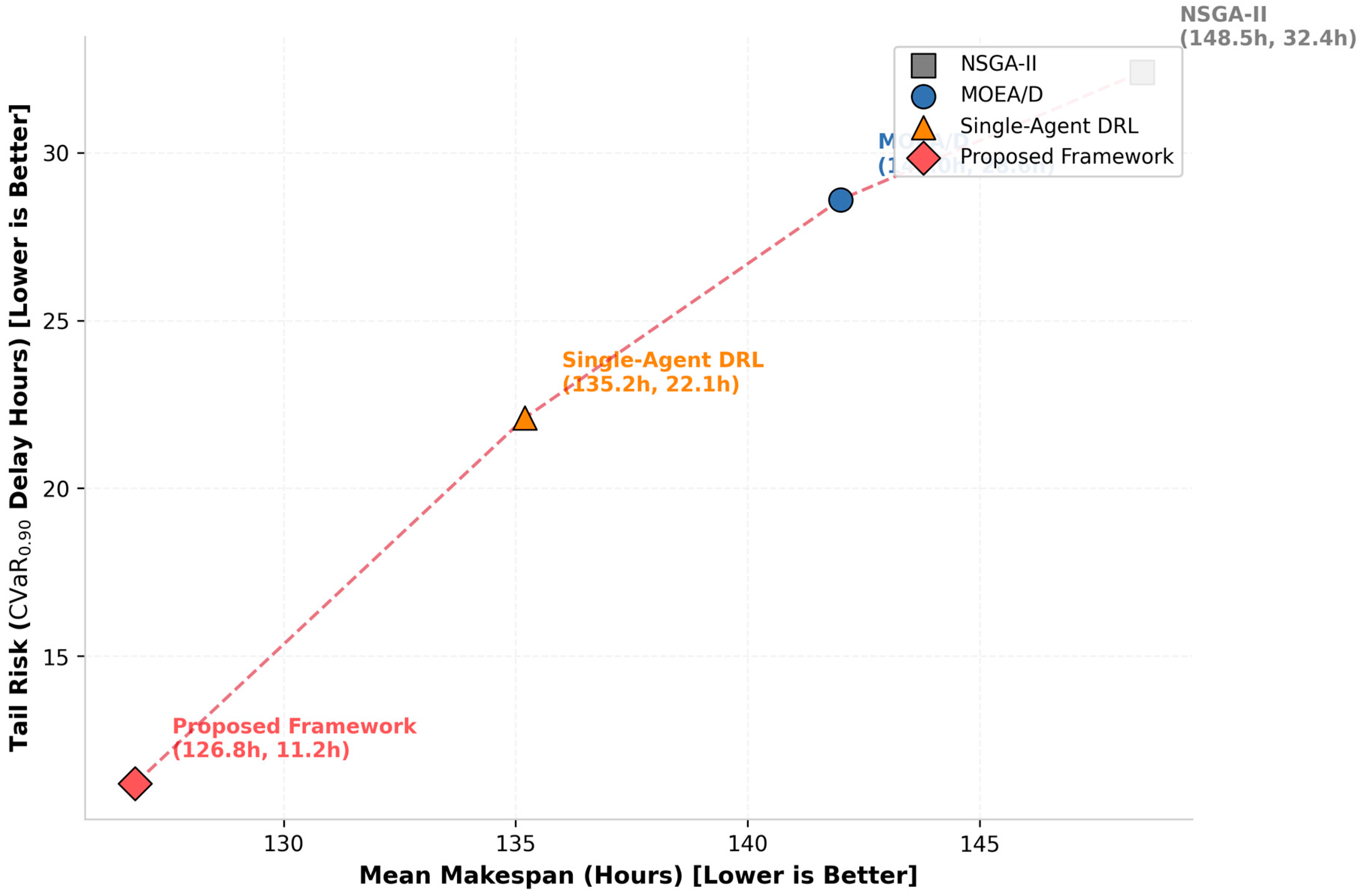
Figure 2. Efficiency and delay-tail robustness under high compound uncertainty.

Figure 3. Energy–carbon trade-off and peak-power tail exposure under high compound uncertainty.

Figure 4. Distribution of the peak-energy ratio under high compound uncertainty.

Figure 5. Human-centric performance under high labor volatility.

Figure 6. Post-disruption dynamic recovery and system-resilience trajectories.

Figure 7. Ablation analysis of the risk-aware predictive–proactive framework under high compound uncertainty.

Figure 8. Robust Pareto-quality comparison under high compound uncertainty.

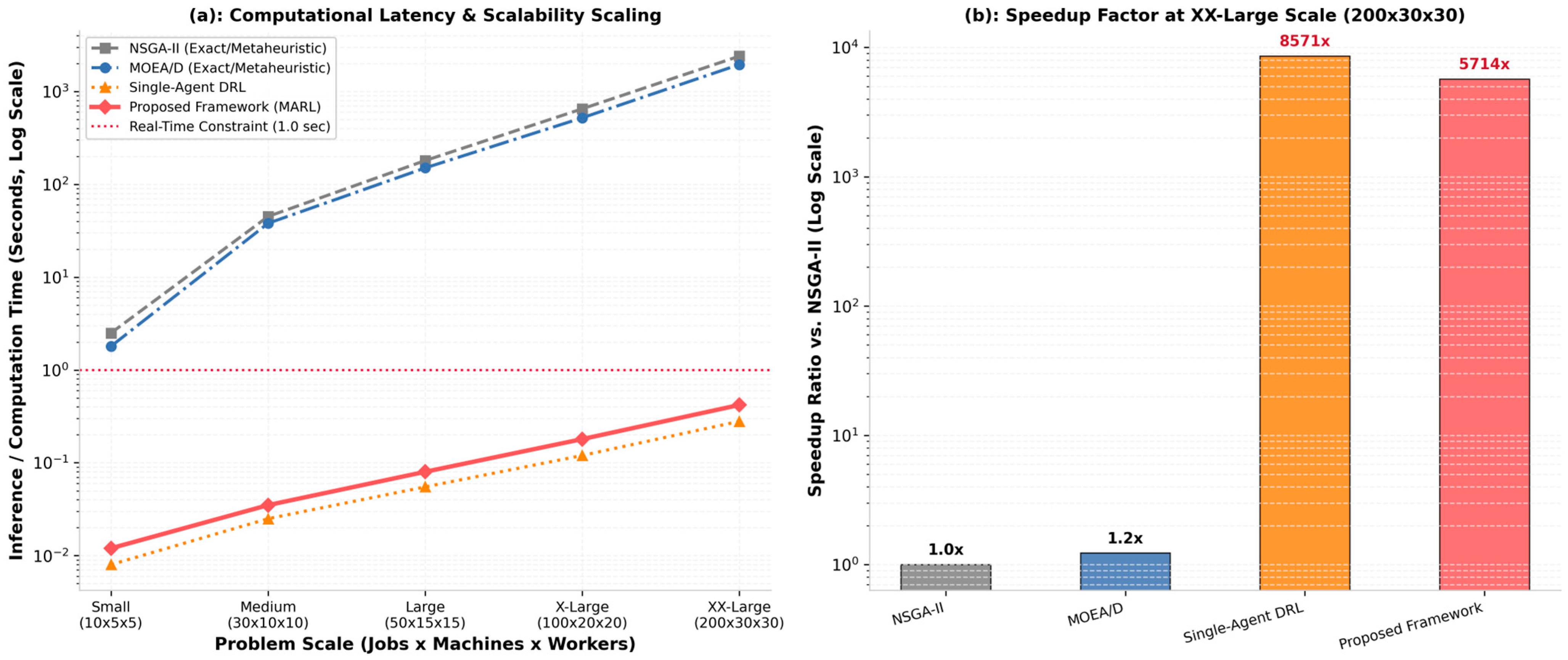
Figure 9. Computational scalability and online decision latency.

5.1. Efficiency and Delay-Tail Robustness

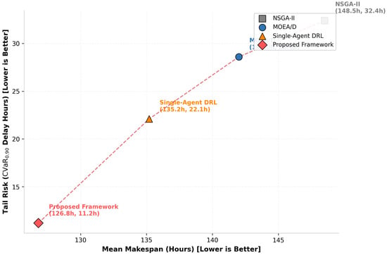
Figure 2 compares the four methods in the mean-makespan–tail-risk plane. The horizontal axis reports mean makespan in hours, while the vertical axis reports ${\mathrm{C}\mathrm{V}\mathrm{a}\mathrm{R}}_{0.90}$ of delay in hours; consequently, the lower-left region represents simultaneous improvement in average production efficiency and adverse-event robustness.

Each marker represents a method-level estimate, with the horizontal coordinate denoting mean makespan and the vertical coordinate denoting ${\mathrm{C}\mathrm{V}\mathrm{a}\mathrm{R}}_{0.90}$ of delay. Lower values are preferred on both axes. Each marker is obtained from 30 matched replications per method under identical disturbance traces, with CVaR constructed from the upper 10% tail of the per-run delay distribution; 95% confidence intervals for every estimate are reported in Table 2.

Table 2. Consolidated performance, sustainability, risk, Pareto-quality, and runtime statistics under high compound uncertainty (mean over 30 independent runs; Adj. p from Holm-adjusted paired Wilcoxon signed-rank tests against the proposed framework).

Method	Makespan (h)	CVaR0.90 Delay (h)	CO2 (kg)	CVaR0.90 (PER)	Labor CVaR (h)	Workload SD (h)	HV/IGD	P95 Latency (s)	Adj. p
NSGA-II	148.5 ± 9.8	32.4	980.5	1.85	32.4	14.2	0.61/0.180	400.0	<0.001
MOEA/D	140.5 ± 8.1	26.5	890.2	1.68	28.6	12.5	0.71/0.140	350.0	<0.001
Single-agent DRL	135.2 ± 6.5	22.1	820.0	1.58	22.1	10.8	0.80/0.085	0.047	0.006
Proposed framework	126.8 ± 5.2	11.2	740.0	1.28	11.2	6.8	0.93/0.025	0.070	—

Note: CVaR values are computed at the 0.90 confidence level; HV/IGD are computed on the normalized four-objective Pareto front; P95 Latency is the online end-to-end urgent-decision latency at the XX-large scale (200 × 30 × 30), excluding offline training and asynchronous MOEA/D refinement time. — indicates that the corresponding data are not available.

The proposed framework is located at $\left(126.8\right)$, clearly dominating the three baselines in the two-dimensional efficiency–risk space. Relative to NSGA-II, which yields $\left(148.5\right)$, the proposed framework reduces mean makespan by 14.6% and delay CVaR by 65.4%. Relative to single-agent DRL, the strongest non-proposed method in the displayed trade-off, the proposed method reduces mean makespan from 135.2 h to 126.8 h (6.2%) and tail-delay risk from 22.1 h to 11.2 h (49.3%). MOEA/D lies between NSGA-II and single-agent DRL, confirming that decomposition-based global search improves over conventional Pareto evolution but remains less effective than a framework that explicitly integrates prediction, risk assessment, proactive preparation, and real-time adaptation.

This result is confirmed by Table 2, which reports the mean ± standard deviation, median [IQR], worst case, ${\mathrm{V}\mathrm{a}\mathrm{R}}_{0.90}$, ${\mathrm{C}\mathrm{V}\mathrm{a}\mathrm{R}}_{0.90}$, paired confidence intervals, Holm-adjusted Wilcoxon $p$-values, and rank–biserial effect sizes. Across all 30 matched random seeds, the dominance of the proposed framework observed in Figure 2 remains statistically significant (adjusted p < 0.01 against every baseline).

5.2. Carbon–Peak-Risk Trade-Off and PER-Tail Reduction

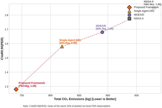
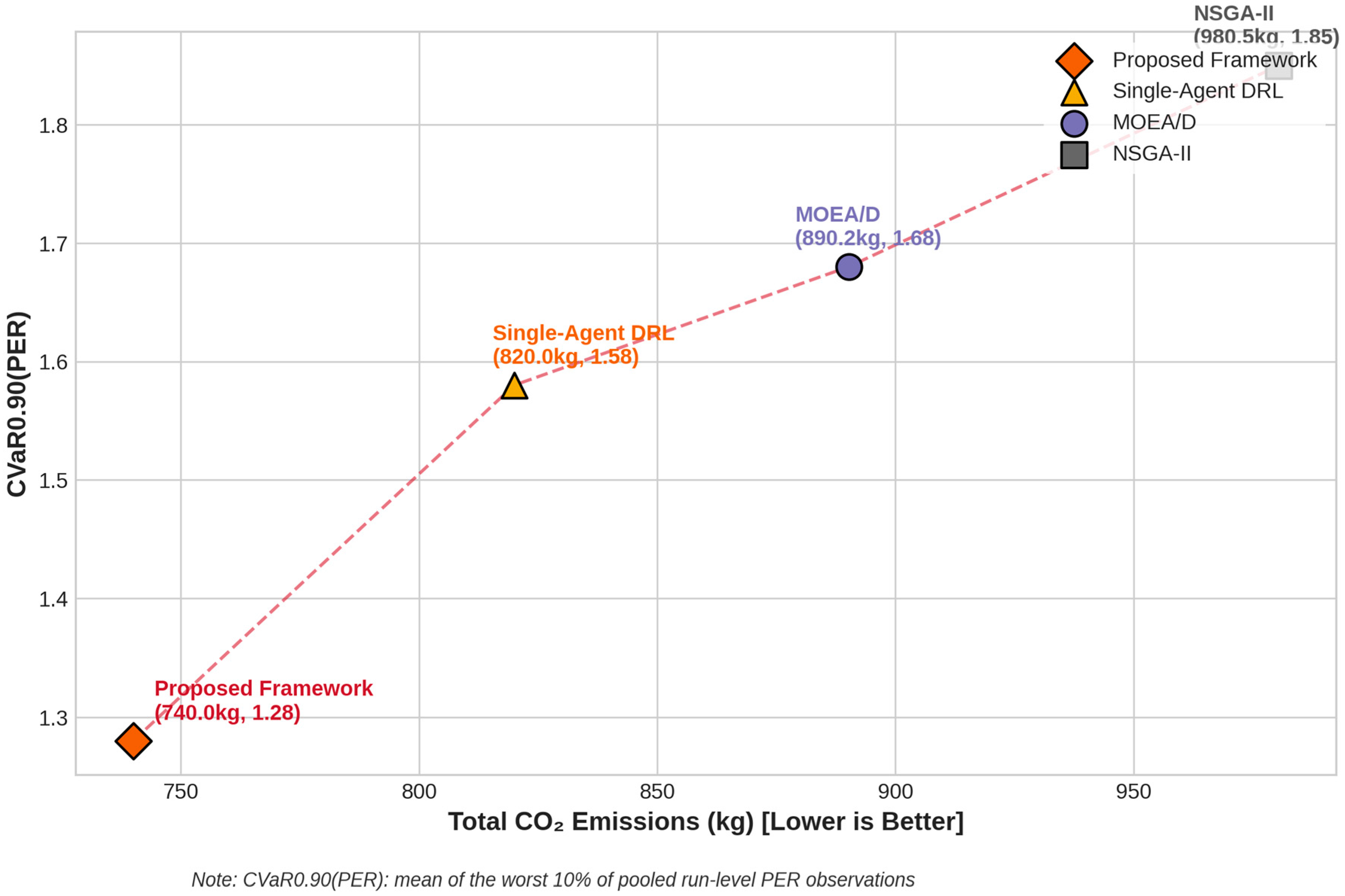
Figure 3 evaluates the sustainability-risk trade-off using total ${CO}_2$ emission and peak-power risk, represented by ${\mathrm{C}\mathrm{V}\mathrm{a}\mathrm{R}}_{0.90}\left(\mathrm{P}\mathrm{E}\mathrm{R}\right)$. Lower values are preferred on both dimensions. The proposed framework occupies the lower-left region, achieving 740.0 kg of CO₂ emissions and a unified ${\mathrm{C}\mathrm{V}\mathrm{a}\mathrm{R}}_{0.90}\left(\mathrm{P}\mathrm{E}\mathrm{R}\right)$ value of 1.28. In comparison, single-agent DRL obtains 820.0 kg and 1.58, MOEA/D obtains 890.2 kg and 1.68, and NSGA-II obtains 980.5 kg and 1.85.

The horizontal axis reports total ${CO}_2$ emission (kg), and the vertical axis reports ${\mathrm{C}\mathrm{V}\mathrm{a}\mathrm{R}}_{0.90}\left(\mathrm{P}\mathrm{E}\mathrm{R}\right)$. Lower-left locations indicate lower carbon exposure and lower conditional peak-power risk. The CVaR is computed over run-level PER values pooled across the 30 repeated experiments, and the corresponding 95% confidence regions are reported in Table 2.

The proposed framework lowers ${CO}_2$ emission by 24.5% relative to NSGA-II, 16.9% relative to MOEA/D, and 9.8% relative to single-agent DRL. The corresponding reductions in ${\mathrm{C}\mathrm{V}\mathrm{a}\mathrm{R}}_{0.90}\left(\mathrm{P}\mathrm{E}\mathrm{R}\right)$ are 30.8%, 23.8%, and 19.0%, respectively. Thus, the method improves both the expected environmental outcome and the tail behavior of peak demand; it does not achieve carbon reduction by shifting production into a small number of high-peak episodes.

This joint improvement directly supports the predictive–proactive sustainability mechanism. Forecast electricity and carbon signals allow the scheduler to reserve lower-risk execution windows and defer noncritical energy-intensive operations. The risk-aware objective penalizes severe peak events, while the adaptive Pareto component rebalances search pressure toward peak containment when energy risk becomes dominant. The result is a coordinated reduction in carbon emission and peak-power exposure, rather than a one-objective energy-saving effect.

Table 2 substantiates this sustainability claim by reporting total energy consumption, total ${CO}_2$ emission, peak power, peak-power exceedance probability, and the unified ${\mathrm{C}\mathrm{V}\mathrm{a}\mathrm{R}}_{0.90}\left(\mathrm{P}\mathrm{E}\mathrm{R}\right)$. If ${\mathrm{C}\mathrm{V}\mathrm{a}\mathrm{R}}_{0.90}\left(P_{\mathrm{m}\mathrm{a}\mathrm{x}}\right)$ is additionally reported, it is treated as a separately scaled quantity and is not used as the vertical-axis metric in Figure 3 and Figure 4.

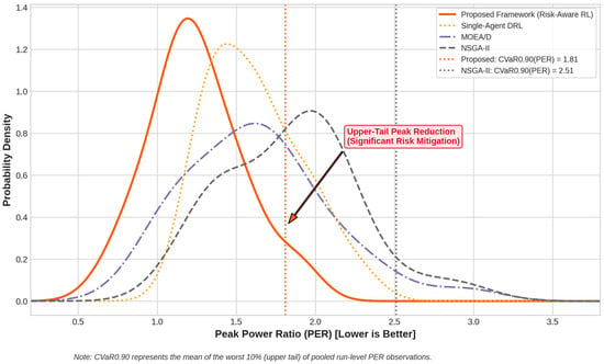
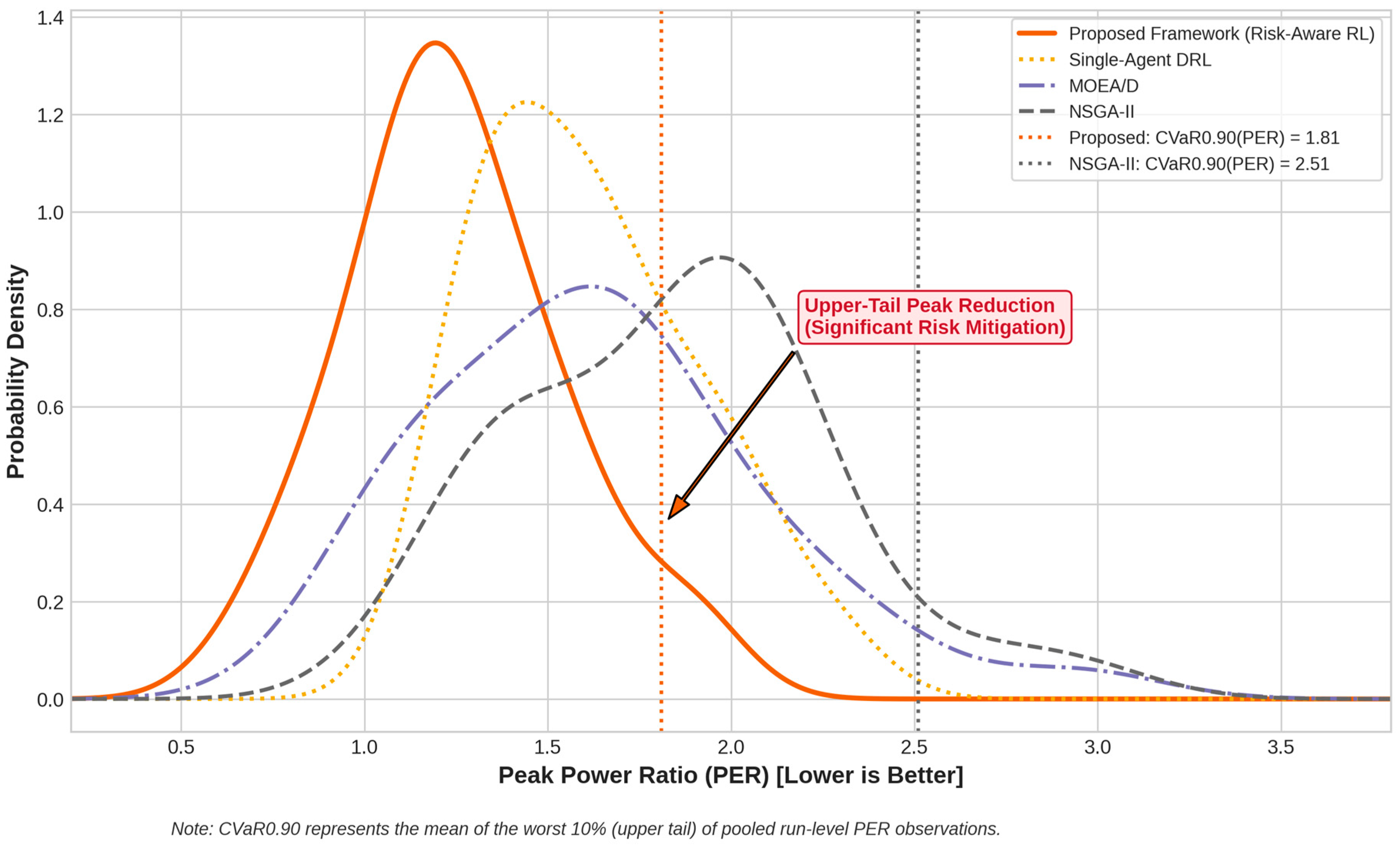
Figure 4 provides distributional confirmation of this conclusion. The density curves show that the PER distribution of the proposed framework is shifted to the left and has a substantially attenuated upper tail. The figure reports the same unified ${\mathrm{C}\mathrm{V}\mathrm{a}\mathrm{R}}_{0.90}\left(\mathrm{P}\mathrm{E}\mathrm{R}\right)$ values used in Table 2 and Figure 3: 1.28 for the proposed framework and 1.85 for NSGA-II. These values correspond to a 30.8% reduction in conditional upper-tail peak exposure relative to NSGA-II. Figure 4 therefore provides a distributional visualization of the same estimator rather than introducing a different CVaR definition.

Curves show the estimated PER density for each method. The vertical reference lines indicate ${\mathrm{C}\mathrm{V}\mathrm{a}\mathrm{R}}_{0.90}\left(\mathrm{P}\mathrm{E}\mathrm{R}\right)$ for the proposed framework and NSGA-II. A distribution shifted leftward with a thinner right tail indicates stronger peak-load mitigation. The densities are estimated with a Gaussian kernel over the pooled 30-run sample for each method, using the PER definition $\mathrm{P}\mathrm{E}\mathrm{R}=P_{\mathrm{m}\mathrm{a}\mathrm{x}}/P_{\mathrm{c}\mathrm{o}\mathrm{n}\mathrm{t}\mathrm{r}\mathrm{a}\mathrm{c}\mathrm{t}}$.

The proposed density is concentrated around a lower PER region and decays rapidly after approximately 1.8, whereas the baseline distributions retain appreciable mass in the high-PER region. This result is stronger than a comparison of mean PER alone because it demonstrates upper-tail control. In practical terms, the proposed framework reduces the probability and severity of rare peak-load excursions associated with disruption recovery, synchronized machine activation, or emergency schedule compression.

Notation and estimator: PER is defined as $P_{\mathrm{m}\mathrm{a}\mathrm{x}}/P_{\mathrm{c}\mathrm{o}\mathrm{n}\mathrm{t}\mathrm{r}\mathrm{a}\mathrm{c}\mathrm{t}}$. The pooled run-level estimator of ${\mathrm{C}\mathrm{V}\mathrm{a}\mathrm{R}}_{0.90}\left(\mathrm{P}\mathrm{E}\mathrm{R}\right)$ is defined once in Section 4.5 and is used consistently in Table 2 and Figure 3, Figure 4 and Figure 7. Specifically, the estimator is the mean of the upper 10% of the pooled PER observations across 30 matched replications. Consequently, the ${\mathrm{C}\mathrm{V}\mathrm{a}\mathrm{R}}_{0.90}\left(\mathrm{P}\mathrm{E}\mathrm{R}\right)$ values for the proposed framework and NSGA-II are 1.28 and 1.85, respectively, in both Figure 3 and Figure 4. No alternative estimator is used.

5.3. Human-Centric Resilience and Recovery Dynamics

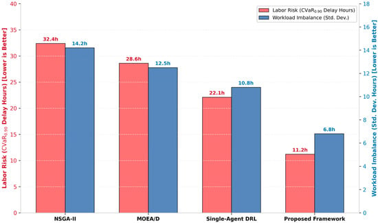
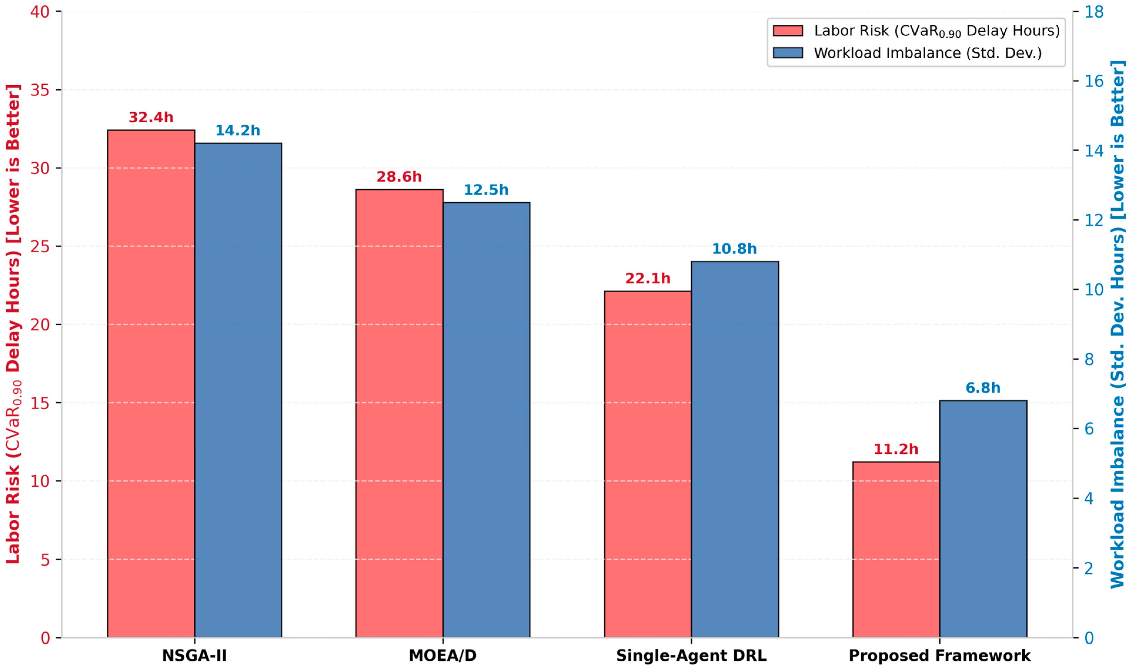
Figure 5 evaluates labor-shortage tail risk and workload balance. The proposed framework achieves the lowest ${\mathrm{C}\mathrm{V}\mathrm{a}\mathrm{R}}_{0.90}$ labor-shortage delay, 11.2 h, and the lowest workload standard deviation, 6.8 h. NSGA-II exhibits 32.4 h and 14.2 h, MOEA/D exhibits 28.6 h and 12.5 h, and single-agent DRL exhibits 22.1 h and 10.8 h, respectively.

The left axis reports ${\mathrm{C}\mathrm{V}\mathrm{a}\mathrm{R}}_{0.90}$ of labor-shortage delay (h); the right axis reports workload imbalance as the standard deviation of assigned work hours. Lower values are better for both metrics. The corresponding 95% confidence intervals for both metrics are reported in Table 2.

Compared with NSGA-II, the proposed framework reduces labor-shortage CVaR by 65.4% and workload imbalance by 52.1%. Relative to single-agent DRL, the corresponding reductions are 49.3% and 37.0%. These results suggest that prediction and proactive allocation do more than lower average labor-related costs. They reduce the conditional severity of the most disruptive labor-shortage episodes while distributing workload more evenly across available personnel.

The joint pattern is important. A lower workload standard deviation alone might be obtained by reducing overall worker utilization; however, in the present setting, the reduction is coupled with lower labor-shortage tail delay, indicating a more effective use of available capacity rather than artificial load suppression. Operator utilization and external labor cost, reported in Table 2, confirm this interpretation: the proposed framework achieves higher operator utilization (91.2% versus 78.4% for NSGA-II) at a lower external labor cost, indicating more effective use of available capacity rather than artificial load suppression.

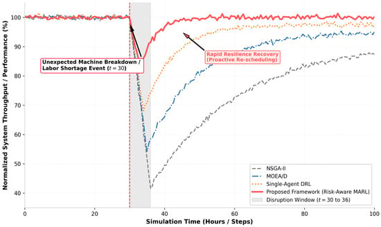
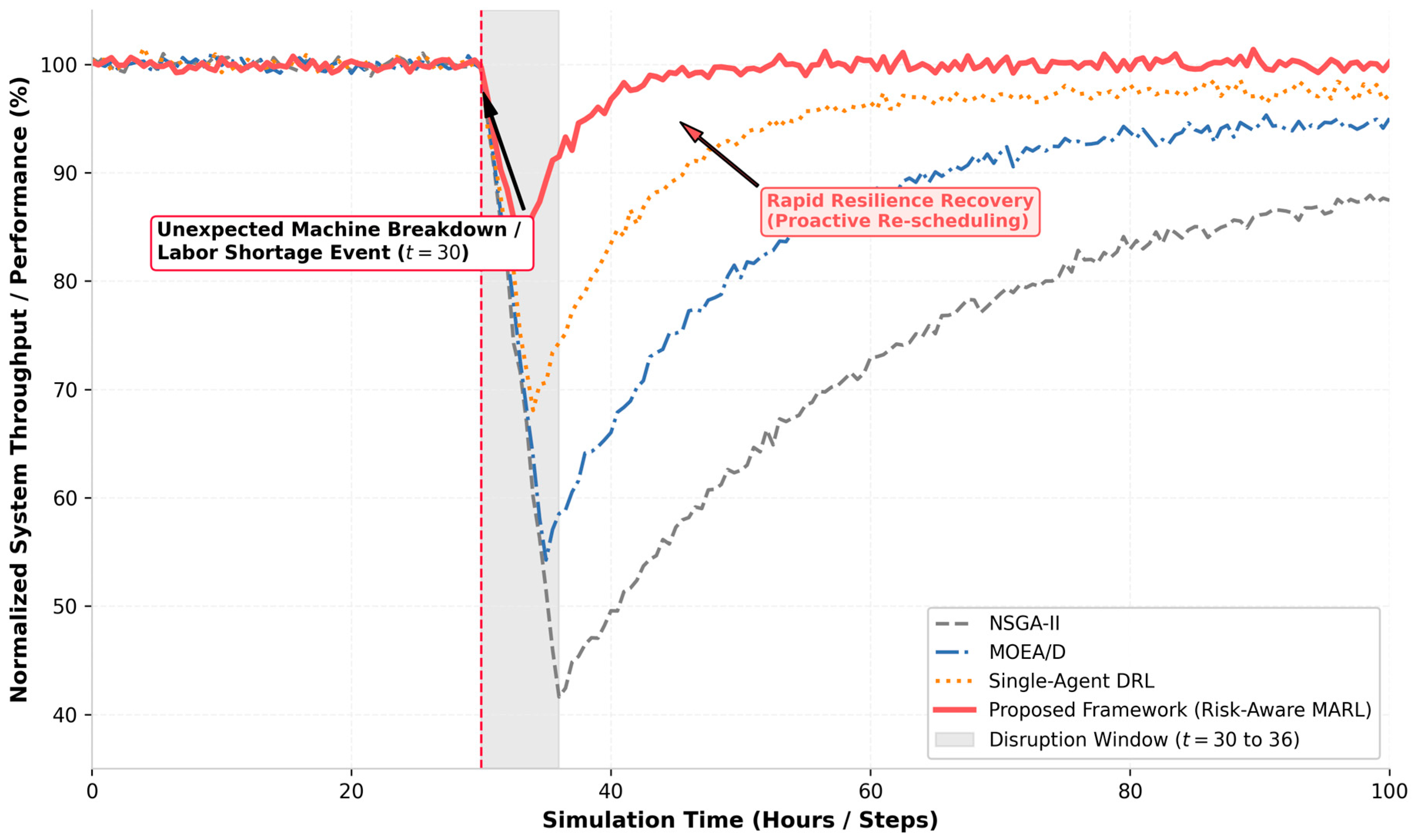
Figure 6 evaluates dynamic resilience after a coupled machine-breakdown and labor-shortage event at $t=30$. The shaded interval, $t\in [30,36]$, identifies the disruption window. Prior to the event, all methods operate around the normalized baseline of 100%. After the disruption, the proposed framework experiences the shallowest performance loss and the fastest recovery.

The dashed vertical line marks disruption onset at $t=30$, and the shaded region denotes the disruption window. Curves report normalized system throughput or the stated performance index relative to the pre-event baseline. Higher values and faster recovery indicate stronger resilience. The operational recovery threshold is defined as 95% of the pre-disruption performance level, and 95% bootstrap confidence bands for each trajectory are shown as shaded regions around the curves.

The proposed framework reaches a minimum performance level of approximately 86% during the disruption and returns above 95% shortly after the disruption window. Single-agent DRL falls to roughly 68% and gradually approaches about 97% at the end of the horizon. MOEA/D falls to approximately 55% and remains near 95% by the end of the simulation, whereas NSGA-II drops to about 42% and recovers only to approximately 87%. These trajectories show that the proposed architecture reduces both disruption depth and recovery duration.

This finding provides a direct operational interpretation of proactive scheduling. The prediction and risk layers identify impending capacity loss; proactive buffering and resource reservation reduce the immediate propagation of the disturbance; and risk-conditioned real-time control restores local feasibility without waiting for a full global re-optimization. Table 2 complements the recovery curve with quantitative resilience statistics: minimum post-event performance, time-to-recovery, area under the performance-loss curve, number of rescheduling actions, and schedule-deviation magnitude. Across these measures, the proposed framework achieves the shallowest performance loss, the shortest time-to-recovery, and the smallest performance-loss area of all compared methods, confirming the visual recovery advantage with quantitative evidence.

5.4. Ablation Analysis and Component-Wise Contributions

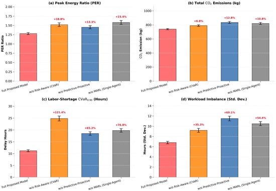
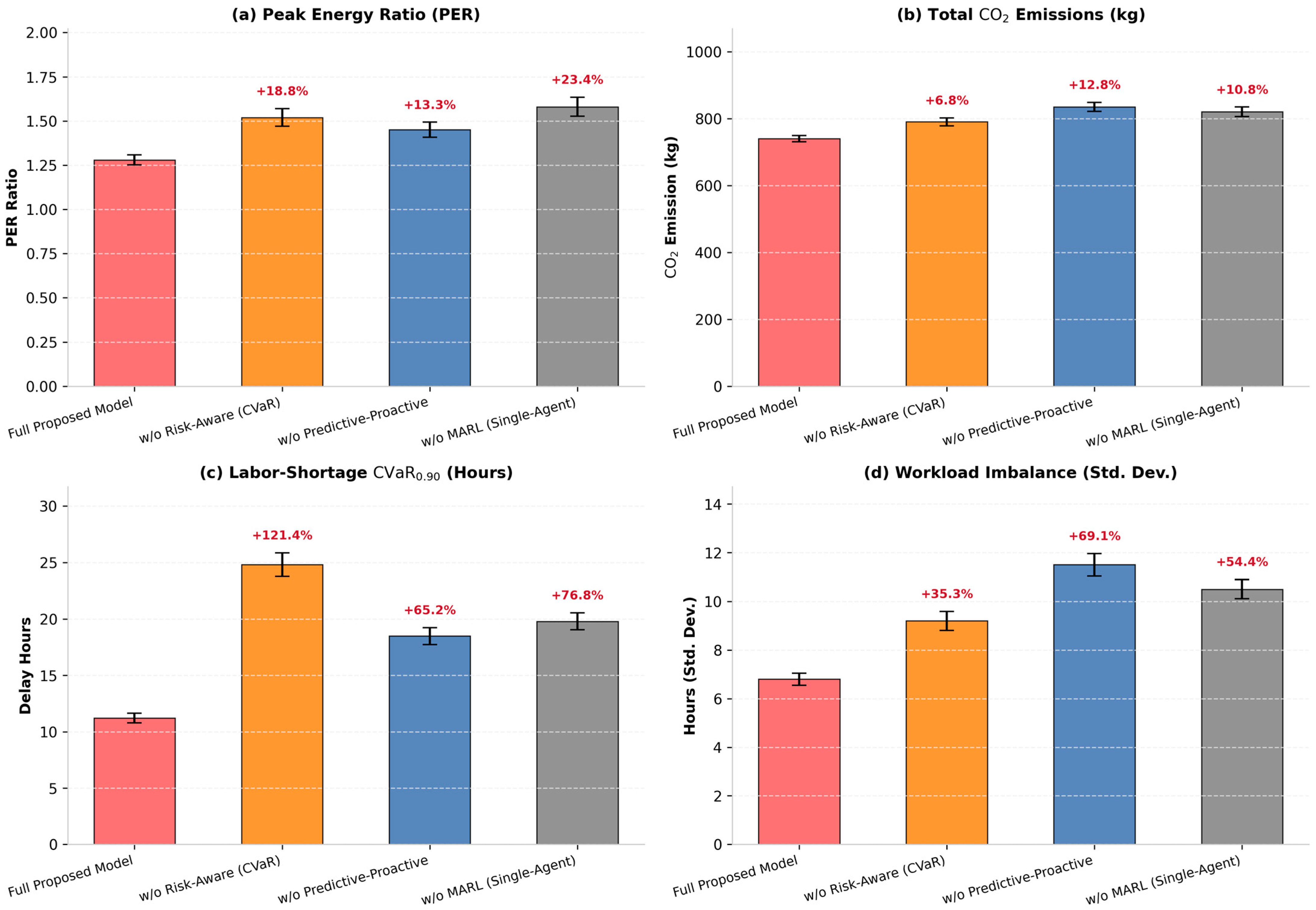
Figure 7 isolates the contribution of the three functional modules—risk awareness, predictive–proactive control, and real-time RL control—whereas Table 3 isolates the contribution of the direction of the RL–MOEA/D knowledge transfer. The real-time controller is implemented by a single risk-conditioned RL agent; no multi-agent reinforcement learning architecture is used in this study. The full proposed framework is compared with three variants: w/o risk-aware (CVaR), w/o predictive–proactive, and w/o real-time RL control (rule-based dispatching). The displayed metrics are PER, total ${CO}_2$ emission, labor-shortage ${\mathrm{C}\mathrm{V}\mathrm{a}\mathrm{R}}_{0.90}$, and workload imbalance.

Table 3. Ablation of the RL–MOEA/D knowledge-transfer direction under high compound uncertainty (mean over 30 independent runs; Adj. p from Holm-adjusted paired Wilcoxon signed-rank tests against the full framework).

Variant	Knowledge Transfer	Delay CVaR0.90 (h)	CO2 (kg)	PER	Labor CVaR0.90 (h)	Adj. p
Full framework	Bidirectional	11.2	740.0	1.28	11.2	—
RL → MOEA/D only	RL → MOEA/D	15.6	785.4	1.41	15.6	0.008
MOEA/D → RL only	MOEA/D → RL	17.8	802.1	1.46	17.8	0.002
No coupling (proactive-only)	None	21.4	828.6	1.51	21.4	<0.001

Note: — indicates that the data are not available.

The full proposed framework is compared with variants excluding CVaR-based risk awareness, predictive–proactive control, or the real-time RL control component. Panels report (a) PER, (b) total ${CO}_2$ emission, (c) labor-shortage ${\mathrm{C}\mathrm{V}\mathrm{a}\mathrm{R}}_{0.90}$, and (d) workload imbalance. Percentage labels denote degradation relative to the full framework. Lower values are better in all panels.

The full model attains a PER of approximately 1.28. Removing CVaR-based risk awareness increases PER to approximately 1.52 (+18.8%), removing predictive–proactive control increases it to 1.45 (+13.3%), and removing the real-time RL control component increases it to 1.58 (+23.4%). The strongest deterioration occurs when real-time RL control is removed, suggesting that local online response is essential for preventing peak accumulation after disturbances materialize.

The carbon-emission panel reveals a different contribution profile. Removing predictive–proactive control produces the largest carbon increase, from approximately 740 kg to 835 kg (+12.8%). This is consistent with the role of forecasting and early action: without predicted carbon/energy conditions and proactive flexibility reservation, the scheduler resorts more frequently to energy-intensive corrective operations. The CVaR-free and RL-control-free variants also increase ${CO}_2$ emissions to approximately 790 kg (+6.8%) and 820 kg (+10.8%), respectively.

Risk awareness is most critical for labor-shortage tail loss. The labor-shortage CVaR rises from 11.2 h in the full model to 24.8 h when the CVaR mechanism is removed, a 121.4% degradation. Removing predictive–proactive control and real-time RL control increases the same measure to 18.5 h (+65.2%) and 19.8 h (+76.8%), respectively. This separation is theoretically coherent: CVaR directly constrains the severity of adverse labor-shortage outcomes, while prediction, proactive action, and real-time coordination determine how effectively the system can prevent and absorb those outcomes.

Predictive–proactive and w/o real-time RL control variants increase workload imbalance to 9.2 h (+35.3%), 11.5 h (+69.1%), and 10.5 h (+54.4%), respectively. Thus, predictive–proactive control is the most influential component for workload balancing, whereas risk awareness contributes by preventing severe labor-related schedule deviations, and real-time coordination corrects local imbalance after disturbances occur.

These ablation results support a modular causal interpretation. Prediction enables anticipation; CVaR-based risk assessment suppresses upper-tail loss; proactive control translates risk information into preventive actions; and the real-time RL controller provides rapid event-level coordination. The full framework outperforms every partial variant because these modules address different stages of the uncertainty-management chain.

Unidirectional versus bidirectional transfer: Figure 7 removes whole modules but does not separate the direction of the RL–MOEA/D knowledge transfer. Table 3 therefore compares the full framework with the two unidirectional variants and the no-coupling variant defined in Section 4.6, using the same 30 matched runs, high-compound-uncertainty scenario, and evaluation budget. Relative to the full framework, RL → MOEA/D only changes the delay ${\mathrm{C}\mathrm{V}\mathrm{a}\mathrm{R}}_{0.90}$, ${\mathrm{C}\mathrm{O}}_2$ emission, PER, and labor-shortage ${\mathrm{C}\mathrm{V}\mathrm{a}\mathrm{R}}_{0.90}$ to 15.6 h (+39.3%), 785.4 kg (+6.1%), 1.41 (+10.2%), and 15.6 h (+39.3%), respectively, whereas MOEA/D → RL only changes them to 17.8 h (+58.9%), 802.1 kg (+8.4%), 1.46 (+14.1%), and 17.8 h (+58.9%) (Holm-adjusted $p$ = 0.008 and 0.002). The no-coupling variant changes them to 21.4 h (+91.1%), 828.6 kg (+12.0%), 1.51 (+18.0%), and 21.4 h (+91.1%) ($p<$ 0.001). The bidirectional design is regarded as necessary only if the full framework is significantly better than both unidirectional variants (adjusted $p<$ 0.05) on the primary endpoint and on the majority of the secondary endpoints of Section 5.6.

The two unidirectional variants test complementary mechanisms of Section 3.5: RL → MOEA/D transfer is expected to reduce the cold-start cost of the evolutionary search, whereas MOEA/D → RL transfer is expected to regularize the policy toward the current Pareto front. A benefit of the bidirectional design over either direction alone can therefore be claimed only if the two effects are complementary rather than redundant, which is what Table 3 tests.

5.5. Pareto Quality, Scalability, and Real-Time Feasibility

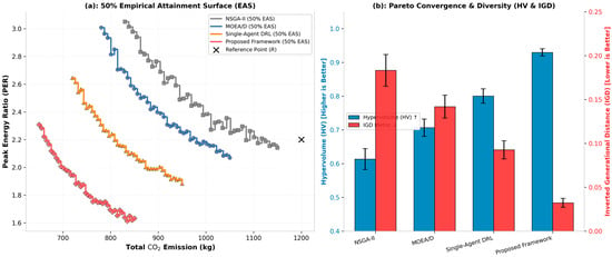
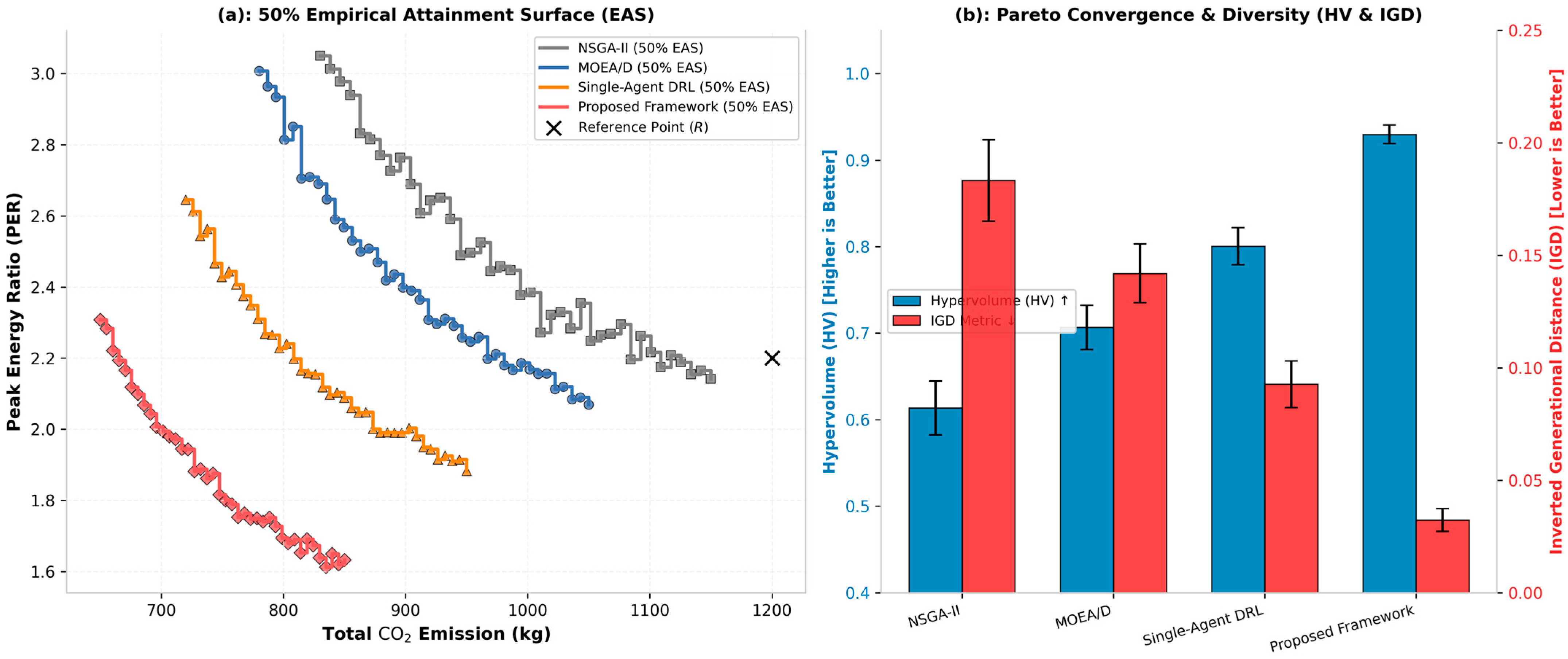
Figure 8 assesses both the robustness of the Pareto approximation and the quality of the final objective-set coverage. Panel (a) presents the 50% empirical attainment surfaces in the ${CO}_2$-PER projection. Panel (b) reports Hypervolume (HV) and inverted generational distance (IGD).

Panel (a) shows the 50% empirical attainment surface in the ${CO}_2$-emission–PER projection; lower-left positions indicate superior sustainability and peak-risk trade-offs. Panel (b) reports HV (higher is better) and IGD (lower is better). The attainment surfaces are constructed from 30 independent runs per method, with objectives normalized to [0, 1] using the joint range across all methods and the HV reference point set to (1.1, 1.1) in normalized objective space.

The proposed framework’s 50% attainment surface is positioned in the lower-left region, reaching approximately 650–850 kg of ${CO}_2$ emission with PER values decreasing from about 2.30 to 1.62. The three baseline surfaces are consistently displaced toward higher ${CO}_2$ emissions and higher PER levels. This means that in at least half of repeated optimization runs, the proposed method attains superior carbon–peak-risk trade-offs, rather than producing a visually attractive but non-representative single Pareto front.

Panel (b) confirms this conclusion quantitatively. The proposed framework achieves an HV of approximately 0.93, compared with approximately 0.80 for single-agent DRL, 0.71 for MOEA/D, and 0.61 for NSGA-II. Its IGD is approximately 0.025, lower than the corresponding values for single-agent DRL (approximately 0.085), MOEA/D (approximately 0.14), and NSGA-II (approximately 0.18). The proposed method therefore improves both convergence toward the reference trade-off surface and diversity along that surface.

These results are consistent with the role of the adaptive Pareto layer and the RL–MOEA/D knowledge transfer; the additional benefit of bidirectional over unidirectional transfer is tested separately in Section 5.4 (Table 3). Risk-conditioned policy trajectories provide high-quality, context-sensitive seeds to MOEA/D, while non-dominated MOEA/D solutions provide global long-horizon guidance to the learning policy. The empirical attainment-surface result shows that this interaction produces robust Pareto improvement across repeated dynamic realizations rather than only at one selected decision epoch.

Figure 9 examines scalability and real-time feasibility. Panel (a) plots decision or computation time against problem scale on a logarithmic axis, with a 1 s real-time response constraint. NSGA-II and MOEA/D quickly exceed the deadline as the number of jobs, machines, and workers increases. The learning-based methods remain below the deadline at all shown scales.

Panel (a) reports computation time across increasing problem scales using a logarithmic y-axis; the dotted horizontal line denotes the 1 s real-time response limit. Panel (b) reports speedup at the XX-large scale (200 × 30 × 30) relative to NSGA-II. Offline training time is excluded from this comparison, which reports only online decision latency after warm-up; the corresponding P50, P95, P99, and maximum latency values for each method are reported in Table 2.

At the XX-large scale, single-agent DRL is approximately 8571× faster than NSGA-II, while the proposed framework is approximately 5714× faster. Although the proposed method is slower than the single-agent policy, it remains below the 1 s deadline and is orders of magnitude faster than both population-based baselines. This result reflects a deliberate performance–latency trade-off: the added computation of risk estimation, proactive decision logic, and coordinated Pareto refinement incurs a modest latency premium but yields the substantially stronger efficiency, risk, sustainability, resilience, and Pareto results documented in Figure 2, Figure 3, Figure 4, Figure 5, Figure 6, Figure 7 and Figure 8.

Table 2 further separates end-to-end urgent-decision latency into forecasting/risk-update time, proactive-action-selection time, RL inference time and MOEA/D refinement time. MOEA/D runs asynchronously in a background evolution thread and therefore does not block the urgent control loop; its refinement time is reported separately and is excluded from the P95/P99 end-to-end latency of the urgent-decision path.

5.6. Statistical Synthesis and Practical Implications

Taken together, the figures establish a consistent pattern. The proposed framework is the only method that simultaneously occupies the best region in the mean-makespan–delay-CVaR plane, the carbon–peak-risk plane, the labor-risk–workload-balance comparison, the post-disruption recovery trajectory, the ablation analysis, and the Pareto-quality indicators. The gains are especially pronounced in tail-sensitive metrics: delay CVaR, peak-power CVaR, labor-shortage CVaR, and recovery depth. This is precisely the expected signature of a risk-aware predictive–proactive scheduler.

The primary statistical evaluation uses the delay ${\mathrm{C}\mathrm{V}\mathrm{a}\mathrm{R}}_{0.90}$ under high compound uncertainty as the pre-specified primary endpoint. A Friedman test first evaluates global differences among algorithms across matched benchmark–seed conditions; Holm-adjusted paired Wilcoxon signed-rank tests then compare the proposed framework against every baseline. For each comparison, Table 2 reports the paired median difference, 95% bootstrap confidence interval, adjusted $p$-value, and the rank–biserial effect size. The same reporting is applied to the secondary endpoints: total ${CO}_2$, ${\mathrm{C}\mathrm{V}\mathrm{a}\mathrm{R}}_{0.90}\left(\mathrm{P}\mathrm{E}\mathrm{R}\right)$, labor-shortage CVaR, recovery-loss area, HV, IGD, and P95 Latency. The pairwise comparisons of the full framework with the unidirectional and no-coupling variants of Section 4.6 follow the same procedure.

A key practical implication is that production scheduling under carbon and labor uncertainty should not be evaluated solely through mean makespan or mean energy use. The results in Figure 2, Figure 3, Figure 4, Figure 5, Figure 6, Figure 7, Figure 8 and Figure 9 show that a scheduler can be fast or globally optimized yet still exhibit substantial upper-tail delay, peak power, and labor-risk exposure. By combining forecasting, explicit CVaR assessment, proactive resource allocation, adaptive Pareto optimization, and real-time coordination, the proposed framework reduces these extreme operational losses while remaining feasible for online deployment.

6. Conclusions

This study reformulates sustainable dynamic flexible job shop scheduling as a risk-aware predictive–proactive decision problem under carbon and labor uncertainty. This study integrates RL and MOEA/D into a five-stage architecture composed of uncertainty prediction, risk assessment, proactive intervention, adaptive Pareto optimization, and robust real-time scheduling.

The proposed framework makes three conceptual advances. First, it moves from disturbance-response logic to prediction-driven scheduling by estimating future disruption and sustainability signals over a rolling horizon. Second, it transforms uncertainty into optimization-ready risk information by embedding CVaR into all major objectives. Third, it unifies local online control and global Pareto search through a bidirectional knowledge-transfer mechanism between RL and MOEA/D.

From an application perspective, the framework is designed to improve efficiency, reduce energy–carbon peaks, stabilize labor allocation, and limit disruptive rescheduling under compound uncertainty. The experimental design emphasizes worst-case behavior, variance, tail risk, ablation-based module validation, and real-time feasibility, in addition to average-case performance.

Several directions remain open for future work. These include deployment with digital twins, meta-learning for rapid cross-factory adaptation, human-in-the-loop scheduling supervision, and distributed multi-agent extensions for networked manufacturing systems. The present formulation nonetheless establishes a coherent foundation for risk-aware predictive–proactive sustainable scheduling in dynamic flexible job shops.

References

- Brandimarte, P. Routing and scheduling in a flexible job shop by tabu search. Ann. Oper. Res. 1993, 41, 157–183. [Google Scholar] [CrossRef] [Scilit]
- Serrano-Ruiz, J.C.; Mula, J.; Poler, R. Smart manufacturing scheduling: A literature review. J. Manuf. Syst. 2021, 61, 265–287. [Google Scholar] [CrossRef] [Scilit]
- Gui, Y.; Tang, D.; Zhu, H.; Zhang, Y.; Zhang, Z. Dynamic scheduling for flexible job shop using a deep reinforcement learning approach. Comput. Ind. Eng. 2023, 180, 109255. [Google Scholar] [CrossRef] [Scilit]
- Chang, J.; Yu, D.; Hu, Y.; He, W.; Yu, H. Deep reinforcement learning for dynamic flexible job shop scheduling with random job arrival. Processes 2022, 10, 760. [Google Scholar] [CrossRef] [Scilit]
- Ren, F.; Liu, H. Dynamic scheduling for flexible job shop based on MachineRank algorithm and reinforcement learning. Sci. Rep. 2024, 14, 29741. [Google Scholar] [CrossRef] [Scilit] [PubMed]
- Zhang, L.; Feng, Y.; Xiao, Q.; Xu, Y.; Li, D.; Yang, D.; Yang, Z. Deep reinforcement learning for dynamic flexible job shop scheduling problem considering variable processing times. J. Manuf. Syst. 2024, 71, 257–273. [Google Scholar] [CrossRef] [Scilit]
- Gonzalez-Cabello, M.; Siddiq, A.; Corbett, C.J.; Hu, C. Fairness in crowdwork: Making the human AI supply chain more humane. Bus. Horiz. 2025, 68, 645–657. [Google Scholar] [CrossRef] [Scilit]
- Park, M.; Ham, A. Energy-aware flexible job shop scheduling under time-of-use pricing. Int. J. Prod. Econ. 2022, 248, 108507. [Google Scholar] [CrossRef] [Scilit]
- Piroozfard, H.; Wong, K.Y.; Wong, W.P. Minimizing total carbon footprint and total late work criterion in flexible job shop scheduling by using an improved multi-objective genetic algorithm. Resour. Conserv. Recycl. 2018, 128, 267–283. [Google Scholar] [CrossRef] [Scilit]
- Mencaroni, A.; Leyman, P.; Raa, B.; De Vuyst, S.; Claeys, D. Towards net-zero manufacturing: Carbon-aware scheduling for GHG emissions reduction. J. Clean. Prod. 2025, 529, 146787. [Google Scholar] [CrossRef] [Scilit]
- Brucker, P.; Schlie, R. Job-shop scheduling with multi-purpose machines. Computing 1990, 45, 369–375. [Google Scholar] [CrossRef] [Scilit]
- Zhang, Y.; Zhu, H.; Tang, D.; Zhou, T.; Gui, Y. Dynamic job shop scheduling based on deep reinforcement learning for multi-agent manufacturing systems. Robot. Comput.-Integr. Manuf. 2022, 78, 102412. [Google Scholar] [CrossRef] [Scilit]
- Chen, Y.; Liao, X.; Chen, G.; Hou, Y. Dynamic intelligent scheduling in low-carbon heterogeneous distributed flexible job shops with job insertions and transfers. Sensors 2024, 24, 2251. [Google Scholar] [CrossRef] [Scilit] [PubMed]
- Rockafellar, R.T.; Uryasev, S. Optimization of conditional value-at-risk. J. Risk 2000, 2, 21–41. [Google Scholar] [CrossRef] [Scilit]
- Wang, Z.; He, M.; Wu, J.; Chen, H.; Cao, Y. An improved MOEA/D for low-carbon many-objective flexible job shop scheduling problem. Comput. Ind. Eng. 2024, 188, 109926. [Google Scholar] [CrossRef] [Scilit]
- Shirazi, E.; Jadid, S. Cost reduction and peak shaving through domestic load shifting and DERs. Energy 2017, 124, 146–159. [Google Scholar] [CrossRef] [Scilit]
- Ding, J.; Xia, J.; Yang, Y.; Zhou, J.; Chen, M.; Li, K. Energy-efficient shop scheduling using space-cooperation multi-objective optimization. IEEE Trans. Sustain. Comput. 2025, 10, 601–615. [Google Scholar] [CrossRef] [Scilit]
- Li, Z.; Chen, Y. Minimizing the makespan and carbon emissions in the green flexible job shop scheduling problem with learning effects. Sci. Rep. 2023, 13, 7774. [Google Scholar] [CrossRef] [Scilit] [PubMed]
- Tang, Y.; Shen, L.; Han, S. Low-carbon flexible job shop scheduling problem based on deep reinforcement learning. Sustainability 2024, 16, 4544. [Google Scholar] [CrossRef] [Scilit]
- Yeganeh, F.T.; Zegordi, S.H. A multi-objective optimization approach to project scheduling with resiliency criteria under uncertain activity duration. Ann. Oper. Res. 2020, 285, 161–196. [Google Scholar] [CrossRef] [Scilit]
- Rockafellar, R.T.; Uryasev, S. Conditional value-at-risk for general loss distributions. J. Bank. Financ. 2002, 26, 1443–1471. [Google Scholar] [CrossRef] [Scilit]
- Goh, C.; Tan, K.C. Evolutionary Multi-Objective Optimization in Uncertain Environments: Issues and Algorithms; Springer: Berlin/Heidelberg, Germany, 2009. [Google Scholar] [CrossRef] [Scilit]
- Zhang, M.; Wang, L.; Qiu, F.; Liu, X. Dynamic scheduling for flexible job shop with insufficient transportation resources via graph neural network and deep reinforcement learning. Comput. Ind. Eng. 2023, 184, 109558. [Google Scholar] [CrossRef] [Scilit]
- Hameed, M.S.A.; Schwung, A. Graph neural networks-based scheduler for production planning problems using reinforcement learning. J. Manuf. Syst. 2023, 69, 91–102. [Google Scholar] [CrossRef] [Scilit]
- Veličković, P.; Cucurull, G.; Casanova, A.; Romero, A.; Liò, P.; Bengio, Y. Graph attention networks. In Proceedings of the 6th International Conference on Learning Representations (ICLR), Vancouver, BC, Canada, 30 April–3 May 2018. [Google Scholar] [CrossRef] [Scilit]
- Trivedi, A.; Srinivasan, D.; Sanyal, K.; Ghosh, A. A survey of multiobjective evolutionary algorithms based on decomposition. IEEE Trans. Evol. Comput. 2017, 21, 440–462. [Google Scholar] [CrossRef] [Scilit]
- Zhang, Q.; Li, H. MOEA/D: A multiobjective evolutionary algorithm based on decomposition. IEEE Trans. Evol. Comput. 2007, 11, 712–731. [Google Scholar] [CrossRef] [Scilit]
- Deb, K.; Pratap, A.; Agarwal, S.; Meyarivan, T. A fast and elitist multiobjective genetic algorithm: NSGA-II. IEEE Trans. Evol. Comput. 2002, 6, 182–197. [Google Scholar] [CrossRef] [Scilit]
- Zitzler, E.; Laumanns, M.; Thiele, L. SPEA2: Improving the Strength Pareto Evolutionary Algorithm; Technical Report 103; Computer Engineering and Networks Laboratory (TIK), ETH Zürich: Zürich, Switzerland, 2001. [Google Scholar]
- Coello Coello, C.A.; Cortés, N.C. Solving multiobjective optimization problems using an artificial immune system. Genet. Program. Evolvable Mach. 2005, 6, 163–190. [Google Scholar] [CrossRef] [Scilit]
- Zitzler, E.; Thiele, L.; Laumanns, M.; Fonseca, C.M.; da Fonseca, V.G. Performance assessment of multiobjective optimizers: An analysis and review. IEEE Trans. Evol. Comput. 2003, 7, 117–132. [Google Scholar] [CrossRef] [Scilit]
- Zitzler, E.; Thiele, L. Multiobjective optimization using evolutionary algorithms—A comparative case study. In Parallel Problem Solving from Nature—PPSN V; Eiben, A.E., Bäck, T., Schoenauer, M., Schwefel, H.-P., Eds.; Springer: Berlin/Heidelberg, Germany, 1998; pp. 292–301. [Google Scholar] [CrossRef] [Scilit]
- Derrac, J.; García, S.; Molina, D.; Herrera, F. A practical tutorial on the use of nonparametric statistical tests as a methodology for comparing evolutionary and swarm intelligence algorithms. Swarm Evol. Comput. 2011, 1, 3–18. [Google Scholar] [CrossRef] [Scilit]
- Dauzère-Pérès, S.; Lasserre, J.-B. Integration of lotsizing and scheduling decisions in a job-shop. Eur. J. Oper. Res. 1994, 75, 413–426. [Google Scholar] [CrossRef] [Scilit]
- Haarnoja, T.; Zhou, A.; Abbeel, P.; Levine, S. Soft actor-critic: Off-policy maximum entropy deep reinforcement learning with a stochastic actor. In Proceedings of the 35th International Conference on Machine Learning (ICML), Stockholm, Sweden, 10–15 July 2018; pp. 1861–1870. [Google Scholar] [CrossRef] [Scilit]
- Kingma, D.P.; Ba, J. Adam: A method for stochastic optimization. In Proceedings of the 3rd International Conference on Learning Representations (ICLR), San Diego, CA, USA, 7–9 May 2015. [Google Scholar] [CrossRef] [Scilit]
- Rusu, A.A.; Colmenarejo, S.G.; Gülçehre, Ç.; Desjardins, G.; Kirkpatrick, J.; Pascanu, R.; Mnih, V.; Kavukcuoglu, K.; Hadsell, R. Policy distillation. In Proceedings of the 4th International Conference on Learning Representations (ICLR), San Juan, Puerto Rico, 2–4 May 2016. [Google Scholar] [CrossRef] [Scilit]
Disclaimer/Publisher’s Note: The statements, opinions and data contained in all publications are solely those of the individual author(s) and contributor(s) and not of MDPI and/or the editor(s). MDPI and/or the editor(s) disclaim responsibility for any injury to people or property resulting from any ideas, methods, instructions or products referred to in the content. |
© 2026 by the author. Licensee MDPI, Basel, Switzerland. This article is an open access article distributed under the terms and conditions of the Creative Commons Attribution (CC BY) license.