


Abstract
This study presents the design, development, and experimental validation of a custom test bench for evaluating the aerodynamic performance of a counter-rotating coaxial propeller system as a function of inter-propeller axial spacing. The experimental campaign was conducted using 254 mm (10 in) GEMFAN 1050 three-blade propellers, representative of small-UAV-scale electric propulsion systems. While prior research has examined coaxial rotor interference effects, systematic experimental studies combining adjustable axial spacing, isolated-rotor baseline measurements, and performance characterization over a broad rotational-speed range remain comparatively limited. The test bench incorporates two BLDC motors instrumented with four strain-gauge load cells, a servo-actuated threaded rod mechanism enabling automated adjustment of rotor spacing, and an RP2040-based dual-core control system for synchronized data acquisition and motor control via DSHOT signaling. The structural frame combines extruded 6063 aluminum profiles, pultruded carbon fiber rods, and 3D-printed polymer components, validated through static and harmonic response finite element simulations. An analytical model based on blade element theory was developed to predict circulation, thrust, power, and induced velocity for each propeller. When evaluated over the experimental rotational-speed range, the analytical thrust prediction showed close agreement with the measured coaxial thrust in the medium-to-high-speed regime, with mean absolute percentage differences of approximately 1.9–2.5% above 5000 rpm across the five tested spacings. Experimental tests were conducted at five axial spacings (70, 90, 110, 130, and 150 mm) across a rotational speed range of approximately 1000–9000 RPM, comparing the coaxial configuration against the summed performance of the two motors operating isolated. Results show that thrust and power curves for the coaxial and isolated configurations remain nearly coincident up to 5000–6000 RPM, beyond which the coaxial system exhibits a measurable thrust deficit driven primarily by aerodynamic interference rather than increased power draw. Coaxial thrust ratios converged toward similar values (~0.83–0.85) at higher rotational speeds regardless of spacing, whereas the largest spacing-dependent differences were observed in the low-to-moderate rotational-speed regime. Because the relative uncertainty of the electrical current measurement increases substantially at low current, the low-throttle thrust-to-power measurements are interpreted as indicative trends rather than as a basis for quantitative ranking of the configurations. These findings provide experimental insight into spacing-dependent interference behavior and establish a validated, low-cost platform for future coaxial rotor characterization studies.
1. Introduction
Coaxial counter-rotating propulsion systems are widely investigated for applications in which high thrust must be generated within a limited projected area. By arranging two propellers along a common axis, the propulsion system can maintain a compact footprint while increasing the available thrust-producing capability. However, the downstream propeller operates within the accelerated and non-uniform flow generated by the upstream propeller, creating aerodynamic interference that affects thrust generation, power consumption, and overall system performance. Experimental and numerical studies have demonstrated that these interactions depend strongly on operating conditions, inflow, and rotor geometry [1,2]. The historical development and aerodynamic particularities of coaxial contra-rotating propulsion systems have also been reviewed extensively, confirming that rotor–rotor interaction remains a central design consideration [3].
Axial separation between the two propellers is one of the principal geometric parameters governing this interaction, yet the literature does not identify a universal spacing that maximizes performance. In the context of heavy-lift UAV design, Ong et al. [4] reported favorable performance for axial separations on the order of 15–20% of rotor diameter in previously investigated configurations. Experimental work on counter-rotating coaxial rotors has further shown that thrust, noise, and overall performance depend strongly on the interaction between the two rotors [5]. Reviews focused specifically on small UAV applications have likewise emphasized the importance of coaxial-rotor spacing, relative rotation, and operating conditions [6]. Hover-performance measurements have also demonstrated that aerodynamic interference in coaxial systems can vary substantially with rotor arrangement and loading [7].
Analytical and reduced-order aerodynamic models provide a complementary means of interpreting these effects. Blade-element and blade-element-momentum approaches offer substantially lower computational cost than high-fidelity CFD and have been extended specifically to coaxial-rotor configurations [8]. Nevertheless, simplified analytical methods cannot fully resolve the development of the upstream wake, radial inflow redistribution, slipstream contraction, or unsteady blade–wake interaction, and therefore require experimental validation. Numerical and experimental investigations of small coaxial multirotor systems have further demonstrated that interaction effects become more pronounced when rotor spacing is reduced [9]. Dedicated experiments on micro-propeller configurations have reported measurable spacing-dependent changes in thrust [10], while investigations of coaxial rotors with independently varied spacing and rotational speed have shown that both parameters can influence total thrust and performance [11]. Studies of variable-spacing coaxial drones similarly indicate that the upper- and lower-rotor characteristics progressively approach isolated-rotor behavior as separation increases [12]. More complex stacked-rotor experiments have additionally demonstrated strong sensitivity to relative axial and azimuthal rotor position [13]. Ducted coaxial configurations likewise show performance penalties associated with aerodynamic interference between the two propulsion units [14], while broader multicopter propulsion studies confirm the importance of evaluating propellers at matched rotational speeds and under well-characterized electrical operating conditions [15].
Reliable experimental characterization therefore requires dedicated test infrastructure. Propeller and rotor test benches have been developed specifically to measure thrust, rotational speed, electrical characteristics, and other propulsion-system quantities for VTOL and UAV applications [16]. More recent experimental rigs have also been designed for both open and shrouded small-scale rotors, emphasizing the need for controlled and repeatable measurement conditions [17]. Commercial and custom coaxial test arrangements have similarly been used to investigate the interaction between front and rear rotors at different separations and rotational speeds [18]. These developments demonstrate the value of configurable test platforms for isolating the influence of rotor spacing from other propulsion-system parameters.
Recent studies further illustrate that preferred spacing is highly dependent on configuration. Li et al. [19] experimentally investigated a ducted coaxial-rotor UAV and identified (H/R = 0.40) as the preferred configuration within their investigated range in terms of thrust and stability, while rotor spacing had only a limited influence on overall propulsive efficiency. Wu et al. [20], using theoretical and computational analyses of a tilt-powered coaxial-rotor UAV, reported (h/R = 0.5) as the best-performing spacing among the configurations examined, with performance decreasing when spacing was increased further. Experimental work on multi-rotor coaxial systems for eVTOL applications has also shown that both rotor count and relative rotation direction affect total system efficiency and the thrust contribution of the downstream rotor [21]. In addition, comparisons involving 10-, 16-, and 26-inch propellers have demonstrated that the performance penalty associated with coaxial operation varies with propeller size and system architecture [22]. Taken together, these results indicate that spacing effects are strongly configuration-dependent and that optimum values obtained for one coaxial system should not be generalized directly to another.
Despite the available literature, relatively few studies combine continuously adjustable axial spacing, isolated-propeller reference measurements, thrust and rotational-speed measurements, and electrical-input characterization using the same propulsion hardware and experimental protocol over a broad operating range. Such a methodology is particularly useful because it allows spacing-dependent interference effects to be distinguished from differences caused by motor, propeller, instrumentation, or operating-condition changes between separate experiments.
The novelty of the present work lies in the integrated use of an automated adjustable-spacing test bench, identical motor–propeller hardware for both isolated and coaxial measurements, direct RPM-resolved comparison over a broad operating range, and an explicit assessment of measurement uncertainty, repeatability, and analytical-model agreement within the same experimental framework.
Accordingly, the present study investigates a counter-rotating coaxial propulsion system using an automated test bench with adjustable axial separation. Five inter-propeller spacings of 70, 90, 110, 130, and 150 mm are examined over an approximately 1000–9000 RPM operating range using the same motor–propeller assemblies and experimental procedure. The objectives of this study are to: (i) develop and structurally assess an automated test platform capable of repeatable coaxial-spacing adjustment; (ii) quantify the influence of axial spacing on thrust and electrical thrust-to-power characteristics; (iii) compare coaxial operation with the corresponding summed isolated-propeller baseline; (iv) assess experimental repeatability and measurement uncertainty; and (v) evaluate the analytical thrust model against the experimental measurements over the investigated rotational-speed range. The purpose is therefore not to establish a universal optimum rotor separation, but to determine the spacing-dependent trends that can be resolved reliably within the geometry and operating envelope investigated in the present study.
2. Materials and Methods
2.1. An Overall View of the Bench
For the development of the experimental test bench designed to evaluate the performance of a coaxial counter-rotating propeller system, materials were selected to provide an optimal balance between structural stiffness, reduced weight, and ease of machining, requirements essential for obtaining accurate and repeatable aerodynamic measurements.
The axial guide rails were manufactured from 20 × 20 mm AA6063 aluminum extrusion profiles. During preliminary bench development, the supporting chassis also used 20 × 20 mm profiles; however, before acquisition of the experimental dataset reported in this study, the main supporting chassis was reinforced using 20 × 40 mm AA6063 aluminum extrusion profiles and steel corner brackets. The 20 × 20 mm guide rails were retained as part of the positioning mechanism. All experimental measurements presented in Section 3 were obtained using this reinforced final configuration. The finite-element analyses described in Section 2.2 concern only the 3D-printed PLA motor-support frames and do not model the aluminum chassis or guide rails.
The two supporting frames were designed to be manufactured by additive manufacturing using PLA. This material was selected due to its ease of fabrication and adequate mechanical properties for the expected loading conditions. The material was modeled with a Young’s modulus of 2600 MPa.
The fixed and mobile motor-support frames were manufactured by fused deposition modeling using PLA. The original detailed printing parameters, including layer height, infill percentage, wall count, nozzle diameter, and build orientation, were not retained in the archived manufacturing documentation and therefore cannot be reported reliably. The components analyzed numerically in Section 2.2 are the same physical motor-support frames used during the experimental campaign.
The 3D model of the coaxial system and the corresponding physical test bench are presented in Figure 1a,b.
Figure 1.
Test bench used in the experiments: (a) 3D model; (b) physical test bench and instrumentation.
The coaxial rotor test rig is constructed around a rigid aluminum extrusion frame reinforced by transverse structural reinforcement rods to prevent mechanical deflection under load, thereby maintaining precise axial alignment between the upper and lower brushless DC (BLDC) motors. Each motor assembly is mounted on elevated platforms supported by load cells, enabling force measurement across both propulsion units.
The DC electrical input to the ESC was externally monitored using a Fluke 381 AC/DC clamp meter (Fluke Corporation, Everett, WA, USA) for current measurement and a Fluke 115 digital multimeter (Fluke Corporation, Everett, WA, USA) for voltage measurement. The detailed measurement procedure, instrument specifications, synchronization with the mechanical measurements, and associated limitations are described in Section 2.3.
The secondary low-voltage auxiliary battery (6–12V) supplies power to the main motherboard and sensors via a step-down buck converter.
Data acquisition is split between the motherboard and the secondary board. The primary motherboard processes raw analog signals from the first pair of load cells and manages central control routines, while a secondary analog-to-digital acquisition module samples signals from the remaining two load cells, transmitting digitized data directly to the motherboard.
Axial adjustment of the distance between the two propellers was achieved using a threaded OLC45 steel rod, enabling accurate and repeatable positioning of the movable assembly. This mechanism allows precise control of the rotor separation distance, which represents the primary parameter investigated in the presented study.
Secondary structural components, including supports, adapters, and sensor mounting elements, were manufactured by fused deposition modeling (FDM) using PLA filament. This manufacturing process enables rapid and cost-effective fabrication of complex geometries while providing sufficient dimensional accuracy for laboratory-scale experimental testing.
The experimental investigations were conducted using GEMFAN 1050 Macroquad 10 × 5 × 3 nylon 12 propellers (Ningbo, China). Owing to its high mechanical strength and excellent fatigue resistance, nylon 12 is well suited for rotor applications subjected to repeated cyclic loading. Furthermore, it is widely recognized as a high-performance thermoplastic for fused filament fabrication (FFF), making it suitable not only for functional prototyping but also for end-use engineering components [23].
The GEMFAN 1050 propeller (Ningbo, China) has a nominal diameter of D = 254 mm and a radius of R = 127 mm. The axial spacing h is defined as the distance measured along the common rotational axis between the planes of rotation of the upstream and downstream propellers. The investigated spacings of 70, 90, 110, 130, and 150 mm therefore correspond to h/D ratios of approximately 0.276, 0.354, 0.433, 0.512, and 0.591, respectively, or equivalently to h/R ratios of approximately 0.55, 0.71, 0.87, 1.02, and 1.18. The investigated interval was specific to the mechanically accessible operating range of the present test-bench configuration and was not intended to establish a universal aerodynamic optimum.
Figure 2 presents two views of the test bench 3D model, including the overall dimensions.
Figure 2.
Test bench with overall dimensions: (a) front view; (b) top view.
During all experimental tests, the propulsion axes were oriented horizontally, such that the principal propeller slipstream developed approximately parallel to the laboratory floor and discharged into open space rather than directly toward the ground. The centerline of both propellers was maintained at a constant height of 218 mm above the floor throughout the complete experimental campaign. For the 254 mm diameter propellers used in this study (R = 127 mm), this corresponds to a normalized centerline clearance of hg/R ≈ 1.72, while the minimum lower blade-tip clearance from the floor was approximately 91 mm (≈0.72R).
Consequently, the present configuration does not correspond to the conventional ground-effect condition associated with a rotor operating with its thrust axis normal to a nearby horizontal surface. Nevertheless, the floor represents the nearest solid boundary and a residual installation or ground-proximity influence on the absolute thrust cannot be completely excluded. Previous work by the authors demonstrated that nearby solid surfaces can modify UAV propeller thrust [24]. Because the rotor height and the surrounding installation were maintained unchanged for all axial-spacing configurations, this boundary condition was common to the complete experimental campaign.
2.2. Structural Analysis of the Fixed and Mobile PLA Motor-Support Frames
The structural integrity of the two 3D-printed PLA motor-support frames, referred to hereafter as the fixed support frame and the mobile support frame, was evaluated using the Simulation Module in Solid Edge 2026. These components are distinct from the aluminum extrusion chassis supporting the overall test bench. The PLA support frames modeled in the finite element analysis are the same motor-support components used during the experimental campaign. Two loading scenarios were considered for each component: a static analysis representing the motor-induced structural loading and a harmonic-response analysis used to identify the dynamic sensitivity of the support frames over the 0–500 Hz frequency range. The material was modeled as PLA with a Young’s modulus of 2600 MPa and a Poisson’s ratio of 0.3.
The harmonic-response calculations used a damping ratio of 0.02. This value was adopted as a numerical modeling assumption and was not obtained from an experimental modal-identification test of the printed components. Consequently, the harmonic analysis is used to identify relative structural sensitivity and potential response peaks rather than to predict experimentally verified vibration amplitudes.
A formal mesh-independence study was not performed for the present structural analysis. Instead, the tetrahedral meshes were locally refined around mounting holes, corners, and other geometric discontinuities where the highest stress gradients were expected. The reported finite-element results should therefore be interpreted as structural design-verification results rather than as mesh-converged high-fidelity predictions.
2.2.1. Fixed Frame
The finite element mesh generated for the fixed frame consisted of 339,882 elements and 513,546 nodes, using an unstructured mesh topology that was locally refined in regions containing fine geometric features, such as holes and corners, to ensure adequate resolution of local stress concentrations. The mesh used in this case is presented in Figure 3.
Figure 3.
Finite element mesh of the fixed frame.
Static Case for the Fixed Frame
The fixed frame was fully constrained at the mounting holes used to secure the frame to the base structure, restricting all translational and rotational degrees of freedom at these locations. A normal force of 12.26 N was applied at each mounting hole corresponding to the motor interface, representing the weight and thrust-induced loading transmitted by the motor assembly.
The simulation results obtained for this case are presented in Figure 4a,b.
Figure 4.
The simulation results corresponding to the fixed frame for the static case: (a) stress distribution; (b) displacement.
The maximum stress reached 9.79 MPa, remaining well below the material’s yield strength of 39.2 MPa. The maximum displacement, equal to 1.21 mm, occurred at the midpoint of the free section of the frame. Under the applied vertical loading, the fixed frame exhibits a safety factor of approximately 4.0 relative to the material’s yield strength, confirming that the fully constrained boundary condition adequately restrains the structure and prevents excessive stress concentration at the mounting interfaces. The maximum displacement was 1.21 mm and occurred at the geometrically most flexible region of the frame. No independent allowable-displacement criterion was defined experimentally for the PLA support components; therefore, the displacement result is reported as a numerical estimate of structural compliance rather than as verification against a prescribed displacement limit. The stress-based assessment remains below the assumed PLA yield strength, with a calculated safety factor of approximately 4.0.
Harmonic Response Case for the Fixed Frame
The same fully constrained condition was applied at the mounting holes as in the static case. However, in this scenario, the excitation force was applied in the tangential direction, at the motor interface, to simulate the dynamic loading generated by rotor operation over a 0–500 Hz frequency sweep, with a damping factor of 0.02.
The simulation results obtained for this case are presented in Figure 5a–c.
Figure 5.
The displacement results corresponding to the fixed frame for the harmonic response case: (a) 0 Hz; (b) 50 Hz; (c) 500 Hz.
The harmonic-response analysis identified a structural response peak near 50 Hz under the assumed tangential harmonic excitation. This frequency corresponds to a one-per-revolution excitation at approximately 3000 RPM; however, this equivalence should not be interpreted as evidence that resonance necessarily occurred during the experiments. The actual dynamic forcing generated by the propulsion system contains several frequency components, including the rotational frequency and blade-passing harmonics. For the three-bladed propellers used here, the blade-passing frequency is three times the rotational frequency and would therefore equal approximately 150 Hz at 3000 RPM. Because the excitation spectrum and operational vibration amplitudes were not measured directly, the harmonic analysis is interpreted as identifying a potential structural sensitivity rather than demonstrating an operational resonance.
2.2.2. Mobile Frame
The finite element mesh generated for the mobile frame consisted of 299,108 tetrahedral elements and 455,442 nodes, similarly, refined in the vicinity of holes and corner regions to accurately capture localized stress gradients. The mesh used in this case is presented in Figure 6.
Figure 6.
Finite element mesh of the mobile frame.
Static Case for Mobile Frame Case
Unlike the fixed frame, the mobile frame boundary conditions were defined to reflect its sliding function within the assembly: the inner surface of the central cylindrical support was fully constrained, while the interfaces in contact with the guide rails were restricted to permit displacement only along the axial direction of the guide rods, with all other translational and rotational degrees of freedom suppressed at these locations. As in the fixed-frame case, a normal static force of 12.26 N was applied at each motor mounting hole. The simulation results obtained for this case are presented in Figure 7a,b.
Figure 7.
The simulation results corresponding to the mobile frame for the static case: (a) stress distribution; (b) displacement.
The maximum stress reached 11.4 MPa, remaining below the assumed PLA yield strength of 39.2 MPa and corresponding to a safety factor of approximately 3.4. The maximum displacement was 0.709 mm, approximately 41% lower than that predicted for the fixed frame. As for the fixed frame, no experimentally established allowable-displacement threshold was available; consequently, the displacement values are used for relative comparison of the structural compliance of the two support designs rather than as verification against a prescribed acceptance limit.
Harmonic Response Case for the Mobile Frame Case
The same boundary conditions were retained as in the static case: full constraint at the central cylindrical support, with normal-only displacement permitted at the guide rail interfaces, while the excitation force was applied in the tangential direction at the motor interface over the 0–500 Hz frequency range, using a damping factor of 0.02. The simulation results obtained for this case are presented in Figure 8a–c.
Figure 8.
The displacement results corresponding to the mobile frame for the harmonic response case: (a) 0 Hz; (b) 50 Hz; (c) 500 Hz.
The displacement increased from 1.41 mm at 0 Hz to a peak of 4.83 mm at the resonant frequency, followed by a continuous decrease down to 0.0203 mm at 500 Hz. The vertically guided boundary condition, in conjunction with the central cylindrical constraint, proves considerably more effective at suppressing resonant amplification under horizontal excitation than the fully constrained condition applied to the fixed frame: the mobile frame’s peak resonant displacement (4.83 mm) is less than half that of the fixed frame (11.8 mm), corresponding to an amplification factor of approximately 3.4× relative to its 0 Hz displacement, compared to nearly 7× for the fixed frame. This indicates that restricting motion exclusively to the vertical (guide rod) direction, rather than fully constraining all degrees of freedom, provides an inherently more favorable dynamic response under tangential dynamic loading, likely due to the additional energy dissipation path introduced by the central cylindrical interface. Nonetheless, the resonant frequency of the mobile frame should be precisely identified and cross-checked against the operational RPM range to fully rule out sustained resonant excitation during testing.
2.3. Method of Measurement
The propulsion system consists of two identical XNOVA Cinelifter Line 3215 430KV BLDC motors controlled by a T-Motor F55A Pro III 4-in-1 ESC (T-MOTOR/Jiangxi Chuangyi Intelligent Technology Co., Ltd., Nanchang, China) and equipped with GEMFAN 1050 Macroquad 10 × 5 × 3 three-blade propellers (Ningbo, China). The propellers have a nominal diameter of 254 mm (10 in), a nominal pitch of 127 mm (5 in), and three blades. Motor M2 is mounted on the fixed support frame and represents the upstream propulsion unit, operating in undisturbed ambient air. Motor M1 is mounted on the mobile support frame and represents the downstream propulsion unit, operating within the slipstream generated by M2 during coaxial operation. Relative to the fixed-frame reference adopted throughout the experiments, the upstream M2 propeller rotates clockwise, whereas the downstream M1 propeller rotates counterclockwise.
The test bench is instrumented with four 5 kg strain-gauge load cells mounted between the motors and the supporting structures, with two load cells assigned to each motor. Each load cell is interfaced through an HX711 24-bit analog-to-digital converter and amplifier module Motor control (Avia Semiconductor (Xiamen) Ltd., Xiamen, China) is achieved through a 4-in-1 ESC (Electronic Speed Controller), of which only two channels are utilized. A central motherboard equipped with an SD (Secure Digital) card reader and a wireless communication module manages data acquisition and system control.
The frame is constructed from extruded aluminum profiles, which serve both as guide rails for the roller mechanism and as mounting points for the 3D-printed frames and carbon fiber rods incorporated to increase structural rigidity, thereby ensuring motor coaxiality and propeller safety. The inter-propeller distance is adjusted by the motherboard via the ESC and servo motor, which rotate a threaded rod analogous to the Z-axis lead screw mechanism commonly used in 3D printers.
To ensure measurement symmetry and to monitor deviations under load, each motor is instrumented with two load cells mounted at its base. Each load cell is connected to a dedicated HX711 ADC/amplifier using the device’s clock/data serial interface. The secondary acquisition board collects the corresponding digitized load-cell measurements and transmits them to the main motherboard through the inter-board communication interface. The HX711 modules themselves use dedicated clock/data interfaces, while communication between the secondary acquisition board and the main motherboard is performed through the I2C bus.
System control is handled by an RP2040 microcontroller unit (MCU) (Raspberry Pi Ltd., Cambridge, UK), implemented on a Raspberry Pi Pico board. Low voltage power (5V) for the board and associated electronics is supplied by a step-down converter, whereas the ESC is powered independently by a 6S LiPo battery with a 120C discharge rating and a 6000 mAh capacity. To ensure consistency across test runs, the battery is recharged and balanced between each experimental trial. The schematic diagram is shown in Figure 9.
Figure 9.
Block diagram of the propulsion-control and data-acquisition system.
All experiments were conducted indoors under nominally quiescent laboratory conditions, with no externally imposed airflow in the test area. Ambient temperature, atmospheric pressure, and relative humidity were not independently logged during the original experimental campaign. Consequently, the analytical calculations employ the standard reference air density of 1.225 kg m−3. The absence of continuously recorded atmospheric conditions is acknowledged as a limitation when interpreting absolute thrust values, although all axial-spacing configurations were tested in the same laboratory environment.
The principal measurement devices used during the experimental campaign, together with their measurement ranges, resolutions, and manufacturer-specified accuracies, are summarized in Table 1. Where a dedicated experimental calibration was performed, the calibration procedure is reported instead of relying exclusively on manufacturer specifications.
Table 1.
Principal measurement devices used during the experimental campaign.
The Fluke 115 digital display provides four updates per second. A numerical display-update rate is not specified by the manufacturer for the Fluke 381; therefore, no unsupported acquisition rate was assigned to the current measurement. Voltage and current readings were recorded during the same stabilized operating condition used for the corresponding thrust and RPM measurements. For the high-resolution 10–40% throttle measurements, a 5 s settling interval preceded acquisition of 700 valid load-cell readings per channel, while the original procedure using 300 readings per channel was retained at higher throttle settings. Because the handheld electrical instruments were not digitally interfaced with the RP2040 acquisition system, electrical and mechanical measurements correspond to the same nominal steady operating condition but are not synchronized at the individual-sample level.
The rotational speed of each BLDC motor was obtained directly from the DShot RPM telemetry provided by the T-Motor F55A Pro III 4-in-1 ESC. The ESC returns electrical rotational-speed information (eRPM), which is converted by the control system to mechanical rotational speed using the configured motor pole count. During coaxial operation, M1 and M2 rotational speeds were acquired independently. For the experimental comparison plots, the rotational-speed coordinate corresponds to the measured coaxial speed, ncoax, calculated as the arithmetic mean of the simultaneously measured M1 and M2 rotational speeds during coaxial operation.
DShot RPM telemetry encodes the electrical rotational period in a 12-bit telemetry field consisting of a 3-bit exponent and a 9-bit mantissa. The encoded electrical period extends from 1 to 65,408 μs, providing substantially finer resolution than required for the rotational-speed range investigated here.
The T-Motor manufacturer does not specify an absolute measurement accuracy for the RPM telemetry of the F55A Pro III ESC; therefore, an unsupported numerical RPM accuracy was not assigned in the present study. This limitation is explicitly acknowledged when interpreting RPM-dependent results.
The electrical input power reported in this study was calculated from the DC-bus voltage and current according to
where UDC and IDC are the voltage and current measured upstream of the ESC. The voltage and current measurements were obtained during the same stabilized operating condition used for the corresponding thrust and RPM measurements. Each operating point was maintained for 7.5 s, allowing the propulsion system and the displays of the Fluke instruments to stabilize before the electrical readings were recorded. The DC electrical input power was then calculated from the corresponding voltage and current values according to PDC = UDCIDC. Because the handheld instruments were not digitally interfaced with the RP2040 acquisition system, voltage and current were not acquired synchronously at the individual-sample level. Accordingly, the reported values represent steady-state DC-bus power estimates associated with the same nominal operating point, rather than instantaneous measurements of v(t)i(t). The electrical instruments were not digitally synchronized sample-by-sample with the RP2040 load-cell acquisition system. Instead, the voltage and current readings were obtained during the same steady operating condition as the corresponding thrust measurement. The duration of each measurement condition depended on the acquisition routine. For the high-resolution 10–40% throttle measurements, a 5 s settling interval was imposed after the commanded operating condition was reached, followed by acquisition of 700 valid load-cell readings per channel with a minimum 25 ms software interval between sampling attempts. At higher throttle settings, the original acquisition procedure used 300 readings per channel. The voltage and current measurements were obtained during the corresponding stabilized operating condition rather than being digitally synchronized with individual load-cell samples. Thus, the electrical and mechanical measurements correspond to the same nominal steady operating point, although they are not time-synchronized at the individual-sample level.
PDC = UDCIDC,
Based on the manufacturer specifications, the limiting electrical measurement is the DC-current measurement, particularly at low current. For the Fluke 381, the specified current accuracy can be expressed as
because five digits correspond to 0.5 A at the 0.1 A resolution. For the Fluke 115 operated on the 60.00 V DC range,
ΔI = 0.02I + 0.5 A
ΔU = 0.005U + 0.02 V
An instrument-specification-based estimate of the relative uncertainty associated with the calculated DC electrical power can therefore be expressed as
The relative uncertainty increases substantially at low throttle because the fixed ±0.5 A component of the clamp-meter specification becomes large relative to the measured current. Consequently, electrical thrust-to-power values obtained at the lowest throttle settings are used only as indicative performance trends and not to establish statistically significant differences between the tested axial spacings.
The RP2040-based control software coordinates motor control, axial-spacing adjustment, sensor acquisition, and SD-card data logging. The test sequence is executed automatically after the target spacing and throttle range are defined, while an emergency stop command permits immediate motor shutdown. Figure 10 summarizes the implemented control sequence.
Figure 10.
Simplified flowchart of the RP2040-based control and data-acquisition software.
Axial spacing was controlled using the servo-driven threaded-rod mechanism with feedback from the VL53L0X Time-of-Flight sensor. The sensor provides a nominal output resolution of 1 mm, while its manufacturer-specified ranging accuracy depends on the selected operating profile. Because the complete mechanical positioning system was not independently calibrated against a higher-accuracy displacement standard, the sensor specification is reported as a sensor-level characteristic rather than as a certified uncertainty of the complete rotor-spacing mechanism.
At each throttle setting, the test sequence begins with the propeller mounted on motor M1 (located on the mobile frame) operating individually, followed by a pause. Motor M2 (located on the fixed frame) is then operated individually, followed by a second pause, after which both propellers are operated simultaneously in the coaxial configuration. For each condition, measurements are acquired only after completion of the programmed settling interval.
The rotation directions were established relative to the fixed frame, considered as the reference frame. The pause interval between successive propeller rotations at a given throttle setting was set to 12 s for throttle values above 40%, and to 17.5 s for throttle values of 40% and below. A 20 s interval is enforced between successive throttle ramps to allow adequate motor cooldown, at the expense of increased total test duration. Once the target distance is defined, the test bench autonomously executes the full testing protocol across all throttle values, encompassing both individual motor tests and coaxial configuration tests, with the bench automatically adjusting its position to match the user-specified distance. Data corresponding to each throttle value are stored as separate files on the SD card. The principal software-control sequence is summarized in Figure 10.
The isolated and coaxial measurements were initially acquired at identical commanded throttle settings. For the final comparison, however, the isolated-rotor measurements were interpolated to the rotational speed measured during the corresponding coaxial operating condition in order to perform the comparison at matched rotational speed. During coaxial operation, the reference rotational speed, ncoax, was defined as the arithmetic mean of the simultaneously measured M1 and M2 rotational speeds.
For each coaxial operating point, the thrust and electrical input power measured during isolated operation of M1 and M2 were linearly interpolated as functions of their respective measured rotational speeds to ncoax. The interpolated isolated values were then summed to obtain the corresponding M1 + M2 baseline at the same rotational speed as the coaxial measurement. Consequently, the coaxial thrust ratio and the electrical thrust-to-power comparisons are evaluated using quantities corresponding to a common rotational speed rather than measurements obtained at slightly different RPM values. Linear interpolation was restricted to the experimentally covered RPM range; no extrapolation beyond the measured isolated-rotor data was performed. This approach is consistent with the equal-RPM comparison methodology reported in [25].
To facilitate comparison between the throttle-based experimental protocol and the RPM-based presentation of the results, Table 2 provides the approximate mapping between commanded throttle and the representative rotational speed nrep across the investigated axial spacings.
Table 2.
Approximate relationship between commanded throttle and measured mean coaxial rotational speed across the investigated axial spacings.
The 100% value is based on the valid available datasets; the 150 mm 100% operating point was not retained in the final dataset.
To provide an independent assessment of the thrust-measurement capability of the newly developed test bench, the isolated-rotor measurements were additionally compared with external static-performance data for an equivalent Gemfan 1050 three-blade propeller. Since the external reference was obtained using a different motor, the comparison was performed as a function of rotational speed rather than throttle command. This approach is supported by previous experimental findings showing that, for a specified propeller, thrust at a given rotational speed is only weakly dependent on the particular motor and battery combination [15]. The detailed comparison is presented in Section 4.5.
2.3.1. Load-Cell Calibration and Uncertainty Assessment
Prior to the experimental campaign, the load-cell measurement channels were calibrated using the same dead-weight procedure previously described in [24]. A reference mass of 2.1 kg was applied to the measurement system to generate a known calibration force, and the corresponding linear calibration coefficient was determined individually for each load-cell channel through the HX711-based acquisition system. The calibration was subsequently verified using additional known weights distributed over the operating range of the test bench. The maximum deviation between the applied reference loads and the measured values remained below 3%, which was adopted as a conservative estimate of the force-measurement uncertainty.
In addition to the calibration assessment, archived experimental records were examined to evaluate run-to-run repeatability. Two independent complete test sweeps were available for an axial spacing of 150 mm. Because the low-throttle acquisition procedure was subsequently modified to increase settling time and the number of acquired samples, only the common 50–90% throttle range of these two original sweeps was used for direct repeatability quantification. For each operating condition, the mean and sample standard deviation of the coaxial thrust and coaxial performance ratio were calculated from the two independent measurements. Owing to the limited number of repeated complete sweeps, these standard deviations are interpreted as an indication of experimental repeatability rather than as a statistically converged estimate of population variance.
The repeatability assessment is therefore based on n = 2 independent complete sweeps at an axial spacing of 150 mm. No equivalent repeated complete sweeps were available for the other four spacing configurations under identical acquisition conditions. Consequently, statistical error bars are reported only where they can be supported directly by repeated measurements; no synthetic uncertainty bars were assigned to the remaining spacing-dependent datasets.
The archived SD-card files contain the processed steady-state result values used for the present analysis rather than the complete sequence of individual load-cell samples acquired internally during each 300- or 700-sample averaging interval. Consequently, the original sample-level signal histories cannot be reconstructed retrospectively for every operating point. The uncertainty analysis is therefore based on the calibration results and on the available independent repeated complete sweeps rather than on a posteriori statistical analysis of individual raw samples.
2.3.2. Data Acquisition and Signal Processing
The four strain-gauge load-cell channels were acquired through individual HX711 24-bit ADC/amplifier modules using a common clock line. The acquisition routine accepted a measurement frame only when all four HX711 channels simultaneously indicated that new data were available. Frames corresponding to invalid all-zero or all-one 24-bit words were rejected before further processing.
For the high-resolution low-throttle measurements at 10%, 20%, 30%, and 40% throttle, the acquisition routine was configured to retain 700 valid readings per load-cell channel. Following application of each commanded motor condition, a 5 s settling interval was imposed before the measurement window was initiated. During acquisition, the software introduced a 25 ms delay between successive sampling attempts. Consequently, the software-limited maximum acquisition rate was approximately 40 samples/s per channel. However, because acceptance of each measurement was additionally conditional on the HX711 data-ready state, the actual effective sampling rate could be lower and was not imposed explicitly by the software. Individual sample timestamps were not retained; therefore, an exact retrospective determination of the effective sampling frequency is not possible.
Load-cell measurements were smoothed using an Exponential Moving Average (EMA) filter applied independently to each channel:
where Xk is the current calibrated load-cell reading, Yk is the corresponding filtered value, and the smoothing coefficient was set to
Yk = αXk + (1 − α)Yk−1
α = 0.12.
The first valid load-cell measurement obtained after the settling period was used to initialize the EMA state. Each subsequent valid sample was filtered using Equation (20), and the final force value associated with the operating point was calculated as the arithmetic mean of the 700 EMA-filtered samples. With the 25 ms software delay, acquisition of 700 accepted measurements required a minimum of approximately 17.5 s, in addition to the preceding 5 s settling interval. The actual acquisition duration could be slightly longer when an HX711 conversion was not yet ready.
No separate digital low-pass filter with an independently prescribed cutoff frequency was implemented in the acquisition firmware. Rather, the EMA operation described above constituted the software low-pass filtering stage. Because the effective sampling frequency was governed jointly by the 25 ms software delay and the HX711 data-ready condition and was not recorded sample-by-sample, a unique experimentally verified cutoff frequency cannot be assigned retrospectively.
At throttle settings above 40%, 300 readings per channel were used in the original acquisition procedure, whereas the 700-reading high-resolution procedure described above was introduced for the 10–40% throttle range to improve the stability of the measurements at low absolute thrust levels.
Only the resulting averaged steady-state load-cell and RPM values were written to the SD-card result files. The individual raw and EMA-filtered sample histories were not retained. Consequently, a retrospective time-domain comparison between raw and filtered signals from the completed experimental campaign cannot be reconstructed. This limitation is explicitly acknowledged, and future implementations of the acquisition system will retain both raw and processed sample histories for direct evaluation of the signal-processing procedure.
2.4. Analytical Approach
The analytical calculations and results are presented below. This section presents the mathematical model developed for the test bench used to predict the circulation, thrust, power delivered to the shaft, and induced velocity of each propeller individually and of the system as a whole.
In order to calculate the force which would later aid in determining the power and velocity of each propeller, first, a circulation of the fluid must be calculated.
The circulation (Γ) quantifies the strength of the vortex flow generated around each blade section and governs the local lift distribution and is dependent upon certain geometric parameters such as:
The analytical formulation follows the blade-element/momentum framework described in [8], adapted here to the geometry of the investigated propeller. The radial coordinate is expressed in dimensionless form as
where r is the dimensional radial coordinate and R1 = 0.127 m is the propeller radius. The lower limit of the aerodynamic blade region is , while the blade tip corresponds to . The representative nondimensional radial position used for evaluation of the blade pitch is .
The remaining parameters are defined as follows: N = 3 is the number of blades; b = 0.023 m is the blade chord; is the nondimensional blade chord; Ω is the angular velocity, with the reference calculation performed at Ω = 994.838 rad/s; τ = 0 is the blade-profile camber angle used in the present model; θ0 = 17.5° is the reference blade angle; and Δθrot = 5° is the blade twist angle. The term appearing in the circulation relation represents the product of the number of blades and the nondimensional chord and is not an independent parameter.
The following equation gives the blade pitch angle:
where
θ0—reference angle for establishing the blade pitch angle (θ0 = 17.5°)
∆θrot—blade twist angle (∆θrot = 5°)
—non-dimensional radius ()
With the blade pitch angle known and with the assumption that the free-stream velocity is zero (V∞ = 0) upon entering the first propeller, a non-dimensional circulation can be evaluated:
The thrust and power integrations are performed over the aerodynamic blade region , i.e., from the nondimensional blade-root location to the blade tip. The rotor disk area used in the momentum relation is .
The value obtained can be utilized to determine the thrust generated (8) and the power absorbed by the shaft (9) by each of the propellers:
where
N—number of blades
—density of air ( = 1.225 )
At this point, the induced velocity, vi, defined as the velocity imparted to the airflow at the propeller disk, can be obtained from momentum theory:
In the case of the second propeller, the assumption that free-stream velocity is zero, (V∞ = 0) is no longer viable since the stream of air coming from the first propeller is at a different velocity than it first was prior to entering the system.
The velocity of the fluid when entering the second propeller is going to be equivalent to the velocity calculated prior.
vi,1 = V∞,2
Since the first case scenario is no longer applicable, the previous zero-inflow formulation used to determine the non-dimensional circulation is no longer applicable and is therefore replaced by:
The formula above does not yield a non-dimensional circulation. Consequently, it is imperative that we perform an additional calculation to make it so:
Because Equation (12) is implicit in Γ, the circulation of the downstream propeller was determined iteratively. The iteration was initialized using the circulation obtained from the zero-inflow solution as the initial estimate. At each iteration, Equation (12) was reevaluated using the circulation obtained from the preceding iteration. Convergence was considered achieved when the absolute change between two successive circulation values satisfied
∣Γ(k+1) − Γ(k)∣ < 10−6.
A maximum of 1000 iterations was imposed to prevent indefinite iteration in the event of non-convergence. The converged dimensional circulation was subsequently converted to its nondimensional form using Equation (13), after which the thrust and shaft power of the downstream propeller were evaluated using Equations (8) and (9).
With the new circulation calculated, by substituting it into (8) and (9), it would follow that the thrust and the power absorbed by the shaft for the second propeller can be determined.
Finally, the induced velocity at the exit of the second propeller is determined (vi,2).
For comparison with the experimental measurements, the analytical model was evaluated over the complete rotational-speed range covered during testing. For the fixed propeller geometry and static operating assumptions considered here, the predicted thrust varies proportionally to the square of rotational speed, while the predicted shaft power varies proportionally to the third power of rotational speed. These relationships are used in Section 4.4 to compare the analytical predictions with the experimental measurements at corresponding rotational speeds. The analytical formulation does not contain axial spacing as an explicit model parameter and is therefore not used to validate the experimentally observed spacing-dependent trends. Its validation is limited to the predicted thrust magnitude and rotational-speed dependence of the coaxial propulsion system.
3. Results
3.1. Reference Analytical Results
The reference analytical solution obtained from Equations (6)–(12) at an angular velocity of 994.838 rad/s, corresponding to approximately 9500 rpm, is presented in Table 3. This reference operating point is subsequently scaled over the complete experimentally investigated rotational-speed range in Section 4.4 for an RPM-matched comparison with the measured coaxial thrust.
Table 3.
Results obtained using analytical relations.
The reference analytical solution predicts lower thrust, shaft power, and circulation for the downstream propeller because it operates within the accelerated inflow generated by the upstream propeller. At the reference condition, thrust decreases from 18.35 N to 10.49 N, while shaft power decreases from 231.85 W to 99.36 W. These results provide the reference solution subsequently used for the RPM-dependent analytical comparison in Section 4.4.
3.2. Experimental Results
This section presents the experimental results obtained for each of the five tested axial spacings of 70, 90, 110, 130, and 150 mm, corresponding to h/D = 0.276, 0.354, 0.433, 0.512, and 0.591, respectively, following the experimental protocol described in Section 2.3. For each configuration, the coaxial system was evaluated against the summed performance of the two propulsion units operating individually over a rotational-speed range of approximately 1000–9000 RPM. The reported quantities comprise thrust, DC electrical input power, electrical thrust-to-power ratio, and the coaxial thrust ratio.
For each measured coaxial operating point, the isolated M1 and M2 thrust values were linearly interpolated to the corresponding measured coaxial rotational speed ncoax.
For each coaxial operating point, the isolated M1 and M2 thrust and electrical-input-power measurements were linearly interpolated, as functions of their respective measured rotational speeds, to the corresponding measured coaxial rotational speed ncoax. The superscript * used below denotes an isolated-rotor quantity evaluated by interpolation at ncoax. The summed isolated-rotor thrust at the matched rotational speed is therefore defined as
where and are the isolated thrust values of M1 and M2, respectively, linearly interpolated to the measured coaxial rotational speed ncoax. The subscript Σ denotes the sum of the two propulsion units, while “iso” denotes isolated operation.
where Tcoax is the measured total thrust with both propellers operating simultaneously at ncoax. A value of ηcoax = 1 indicates that the coaxial thrust equals the summed isolated thrust interpolated to the same rotational speed, while values below unity indicate a coaxial thrust deficit.
For the electrical measurements, the summed isolated electrical input power and the coaxial electrical input power are defined as
where and are the isolated electrical input powers of M1 and M2, respectively, linearly interpolated to ncoax. At each measured isolated operating point, electrical input power was first calculated as P = UI from the corresponding measured DC voltage and current, after which the resulting power values were interpolated as a function of rotational speed.
And
where Ucoax and Icoax are the DC-bus voltage and current measured during simultaneous coaxial operation, and Pcoax is the corresponding coaxial electrical input power.
Pcoax = UcoaxIcoax
The corresponding electrical thrust-to-power ratios are
And
where KT/P,iso and KT/P,coax denote the electrical thrust-to-power ratios of the isolated and coaxial configurations, respectively. These quantities are expressed in g/W and therefore represent dimensional propulsion-performance metrics rather than thermodynamic efficiencies.
Both electrical thrust-to-power ratios are expressed in g/W and represent system-level propulsion metrics rather than dimensionless thermodynamic efficiencies. Owing to the electrical-instrument uncertainty discussed in Section 2.3, quantitative comparisons at the lowest throttle settings are interpreted cautiously.
3.2.1. Experimental Results for a Distance Between the Two Propellers of 70 mm
At 70 mm (h/D = 0.276), the coaxial and summed isolated thrust curves remain close up to approximately 5000–6000 RPM and diverge progressively at higher rotational speeds. The corresponding electrical input-power curves remain comparatively close over the investigated range. The coaxial thrust ratio exhibits its lowest value at the first measured operating point and subsequently approaches approximately 0.83–0.85. Because the first point lies in the low-thrust regime, where relative measurement uncertainty is greatest, it is retained as an experimental measurement but is not used independently to rank the investigated spacings. The results can be observed in Figure 11.
Figure 11.
Experimental results obtained at an axial spacing of 70 mm (h/D = 0.276) after RPM matching of the isolated and coaxial operating conditions: (a) coaxial thrust and summed isolated thrust interpolated to the measured coaxial rotational speed, ncoax; (b) coaxial electrical input power and summed isolated electrical input power interpolated to ncoax; (c) electrical thrust-to-power ratio of the coaxial configuration; (d) coaxial thrust ratio calculated using the RPM-matched isolated baseline.
3.2.2. Experimental Results for a Distance Between the Two Propellers of 90 mm
At 90 mm (h/D = 0.354), the overall behavior is similar to that observed at 70 mm. The coaxial and summed isolated thrust curves remain close at low-to-moderate RPM and separate at higher rotational speeds, while the electrical input-power curves show a smaller relative difference. The coaxial thrust ratio exhibits several localized variations before approaching approximately 0.82–0.85 at higher RPM. Because these point-to-point variations are comparable to the experimental repeatability reported in Section 3.3, they are treated as experimental scatter rather than as evidence of a distinct aerodynamic transition. The results can be observed in Figure 12.
Figure 12.
Experimental results obtained at an axial spacing of 90 mm (h/D = 0.354) after RPM matching of the isolated and coaxial operating conditions: (a) coaxial thrust and summed isolated thrust interpolated to the measured coaxial rotational speed, ncoax; (b) coaxial electrical input power and summed isolated electrical input power interpolated to ncoax; (c) electrical thrust-to-power ratio of the coaxial configuration; (d) coaxial thrust ratio calculated using the RPM-matched isolated baseline.
3.2.3. Experimental Results for a Distance Between the Two Propellers of 110 mm
At 110 mm (h/D = 0.433), the coaxial and summed isolated thrust curves again diverge progressively above approximately 5000–6000 RPM. The 110 mm configuration exhibits the highest measured coaxial thrust-ratio values in the low-speed portion of the present dataset. However, this region also corresponds to greater relative measurement uncertainty, and independent repeated sweeps were not available for this spacing. The result is therefore interpreted as an observed experimental trend rather than as evidence of a statistically demonstrated optimum. At higher rotational speeds, the coaxial thrust ratio converges toward approximately 0.83–0.84. The results can be observed in Figure 13.
Figure 13.
Experimental results obtained at an axial spacing of 110 mm (h/D = 0.433) after RPM matching of the isolated and coaxial operating conditions: (a) coaxial thrust and summed isolated thrust interpolated to the measured coaxial rotational speed, ncoax; (b) coaxial electrical input power and summed isolated electrical input power interpolated to ncoax; (c) electrical thrust-to-power ratio of the coaxial configuration; (d) coaxial thrust ratio calculated using the RPM-matched isolated baseline.
3.2.4. Experimental Results for a Distance Between the Two Propellers of 130 mm
At 130 mm (h/D = 0.512), the thrust and electrical-input-power trends remain consistent with those obtained at the smaller axial spacings. The coaxial thrust ratio contains several local increases and decreases over the investigated range, but their magnitude is comparable to the measured repeatability spread. These variations are therefore interpreted conservatively as experimental variability. At higher RPM, the values converge toward the same general range observed for the other spacing configurations. The results can be observed in Figure 14.
Figure 14.
Experimental results obtained at an axial spacing of 130 mm (h/D = 0.512) after RPM matching of the isolated and coaxial operating conditions: (a) coaxial thrust and summed isolated thrust interpolated to the measured coaxial rotational speed, ncoax; (b) coaxial electrical input power and summed isolated electrical input power interpolated to ncoax; (c) electrical thrust-to-power ratio of the coaxial configuration; (d) coaxial thrust ratio calculated using the RPM-matched isolated baseline.
3.2.5. Experimental Results for a Distance Between the Two Propellers of 150 mm
At 150 mm (h/D = 0.591), the maximum experimentally reached rotational speed was lower than for the other spacing configurations. Consequently, the lower maximum thrust measured for this case should not be attributed to axial spacing alone. The coaxial thrust ratio exhibits several localized variations, including a decrease near 7000 RPM. Because repeatability measurements for this spacing demonstrate that variations of a few hundredths can occur between independent runs, these local changes are treated as experimental scatter and are not attributed to resonance, wake transitions, or other specific aerodynamic mechanisms without additional supporting measurements. The results can be observed in Figure 15.
Figure 15.
Experimental results obtained at an axial spacing of 150 mm (h/D = 0.591) after RPM matching of the isolated and coaxial operating conditions: (a) coaxial thrust and summed isolated thrust interpolated to the measured coaxial rotational speed, ncoax; (b) coaxial electrical input power and summed isolated electrical input power interpolated to ncoax; (c) electrical thrust-to-power ratio of the coaxial configuration; (d) coaxial thrust ratio calculated using the RPM-matched isolated baseline.
Furthermore, to compare the measured performance across the investigated axial-spacing range, the results obtained for the five configurations were plotted together, as shown in Figure 16.
Figure 16.
Comparison across the five tested axial spacings after RPM matching of the isolated and coaxial operating conditions, h/D = 0.276, 0.354, 0.433, 0.512, and 0.591: (a) coaxial thrust ratio calculated using the isolated thrust interpolated to the measured coaxial rotational speed, ncoax; (b) electrical thrust-to-power ratio of the coaxial configuration as a function of ncoax.
Figure 16 and Table 4 show that axial spacing has its largest measured influence in the low-speed portion of the dataset. The 110 mm configuration exhibits the highest measured coaxial thrust-ratio values in this region, whereas the 70 mm configuration exhibits the lowest measured values. However, because this region is associated with greater relative measurement uncertainty and complete independent repetitions were not available for all spacings, this ordering is treated as an indicative trend rather than as a statistically established ranking.
Table 4.
Summary of the experimental spacing configurations after RPM matching of the isolated and coaxial operating conditions.
Above approximately 4000–5000 RPM, the coaxial thrust-ratio curves converge toward approximately 0.82–0.85, and the remaining differences between spacing configurations are comparable in magnitude to the run-to-run variation observed in the separate 150 mm repeatability assessment; this comparison is used only as an approximate transferred estimate. Consequently, no statistically meaningful high-RPM ranking is inferred. Similarly, localized variations of only a few hundredths in ηcoax are treated as experimental scatter rather than as evidence of specific wake transitions or structural resonance.
3.3. Run-to-Run Repeatability
To assess the repeatability of the experimental measurements, two independent complete test sweeps available in the archived dataset for an axial spacing of 150 mm were compared. Since the low-throttle acquisition procedure was subsequently modified by increasing the settling duration and the number of acquired samples, the repeatability assessment was restricted to the common 50–90% throttle range, for which both runs were obtained using the same acquisition procedure. The comparison focused on coaxial thrust and the coaxial thrust ratio, ηcoax, as these quantities are directly relevant to the evaluation of aerodynamic interference between the two propellers.
For each throttle setting, the two independent measurements are reported directly as an observed run-to-run range. Because only two complete repeated sweeps were available, no sample standard deviation or confidence interval is used to characterize dispersion. The range therefore represents the difference between the two measured values and is used only as an empirical indication of the run-to-run variability of the test bench.
The measurements range are regarding the throttle are presented in Table 5.
Table 5.
Run-to-run repeatability for the 150 mm axial-spacing configuration.
Because only two independent complete sweeps were available, the reported sample standard deviations are used as repeatability indicators and are not interpreted as statistically converged estimates of population uncertainty; 95% confidence intervals were therefore not reported. A better visualization of the sweeps is presented in Figure 17.
Figure 17.
Run-to-run repeatability assessment at an axial spacing of 150 mm over the common 50–90% throttle range: (a) coaxial thrust; (b) coaxial thrust ratio, ηcoax. The two independent test runs are shown together with their mean values; error bars represent the half-range between the two measurements and are used only as an empirical indication of run-to-run variability.
Across the common 50–90% throttle interval, the difference between the two measured coaxial-thrust values ranged from approximately 15.3 to 59.9 gf, corresponding to a relative run-to-run difference of approximately 1–3% of the mean thrust level. The observed ηcoax ranges were 0.843–0.853, 0.839–0.840, 0.808–0.827, 0.823–0.831, and 0.817–0.845 at 50%, 60%, 70%, 80%, and 90% throttle, respectively.
Because only two complete repeated sweeps were available, these ranges are interpreted only as an empirical estimate of the order of run-to-run variability and not as a statistically converged uncertainty measure.
These results indicate that the experimental bench provides good run-to-run repeatability in the medium-to-high throttle range. However, the observed variability in ηcoax also demonstrates that differences of only a few hundredths between individual spacing configurations can be comparable to the experimental repeatability spread. Consequently, small localized differences between the ηcoax curves should be interpreted cautiously and should not, by themselves, be considered evidence of a distinct aerodynamic interference regime.
The repeatability assessment was obtained only for the 150 mm spacing and over the common 50–90% throttle interval. Consequently, the observed run-to-run range should not be interpreted as a directly measured uncertainty bound for the 70, 90, 110, or 130 mm configurations, particularly in the low-throttle region. Where this repeatability range is referenced elsewhere in the manuscript, it is used only as an approximate indication of the order of experimental scatter transferred from a different spacing and operating range.
These repeated sweeps were obtained for the 150 mm spacing and therefore quantify the order of experimental run-to-run variability of the test bench, but they do not constitute a direct repeatability assessment of the 110 mm low-speed measurements.
4. Discussion
The discussion focuses on the principal limitations and validation results relevant to the interpretation of the experimental measurements: signal acquisition and low-throttle uncertainty, structural and thermal behavior of the test bench, analytical–experimental comparison, and independent validation of the thrust measurements.
4.1. Influence of Data Acquisition on Measurement Interpretation
The acquisition and signal-processing procedure is described in Section 2.3.2. The increased number of acquired samples used in the 10–40% throttle range was introduced because the smaller absolute load-cell signals in this region are more sensitive to measurement fluctuations. Consequently, relatively small differences between axial-spacing configurations at low rotational speeds should be interpreted cautiously.
The archived experimental files contain the processed steady-state results rather than the complete individual sample histories. Therefore, the effect of the EMA filter cannot be re-evaluated retrospectively using raw time-domain measurements from the completed experimental campaign. This limitation will be addressed in future implementations by storing both raw and filtered load-cell samples.
4.2. Thermal Management
Thermal monitoring showed a maximum motor-stator temperature of approximately 86 °C during extended testing. The upstream motor operated up to approximately 15 °C hotter than the downstream motor, which was exposed to the accelerated slipstream. Cooldown intervals were therefore incorporated between successive operating conditions to limit thermal accumulation.
4.3. Structural Rigidity and Final Experimental Configuration
Preliminary mechanical evaluations performed during development of the test bench showed that torsional compliance of the original aluminum support structure could induce transient zero-point shifts in the load-cell signals when the bench was externally disturbed. Consequently, before acquisition of the experimental dataset reported in this study, the aluminum chassis was reinforced using 20 × 40 mm extrusion profiles and steel corner brackets. All measurements presented in Section 3 were obtained with this reinforced chassis on a leveled surface and without physical contact with the structure during automated testing.
This modification concerned the aluminum supporting chassis and should not be confused with the fixed and mobile 3D-printed PLA motor-support frames analyzed in Section 2.2. Those PLA components were retained in the experimental configuration and correspond to the components represented in the finite element analyses.
The experimental thrust and power curves were also examined in the vicinity of approximately 3000 RPM, corresponding to the 50 Hz one-per-revolution frequency identified in the harmonic analysis. No systematic discontinuity or anomalous increase was observed across the five spacing configurations that could be uniquely associated with structural resonance. Some point-to-point variation is present in this region, particularly in the coaxial thrust ratio; however, as discussed in Section 3.3, variations of this magnitude are comparable to the measured experimental repeatability and are therefore not attributed to structural resonance. Dedicated vibration measurements would be required to establish whether the 50 Hz structural mode is significantly excited during operation.
For this reason, measurements obtained near 3000 RPM, including those for the 110 mm spacing, are not interpreted as evidence of either a structural-resonance effect or a uniquely favorable aerodynamic condition.
4.4. Comparison Between Analytical and Experimental Thrust Results
The analytical–experimental comparison was performed at corresponding rotational speeds rather than by directly comparing the 9500 RPM reference calculation with measurements obtained at lower rotational speeds. The analytical solution obtained at 9500 RPM was therefore scaled over the experimentally investigated RPM range using the quadratic thrust and cubic shaft-power dependencies defined below. The experimental rotational speed used for the comparison corresponds to the measured coaxial rotational speed, ncoax, defined in Section 2.3 as the arithmetic mean of the simultaneously measured M1 and M2 rotational speeds during coaxial operation. This procedure permits assessment of the predicted thrust magnitude and rotational-speed dependence of the analytical model. However, because axial spacing is not an explicit parameter of the analytical formulation, the comparison is not intended to validate the experimentally measured variation in performance with rotor separation.
For the fixed propeller geometry and operating assumptions considered in the analytical formulation, the non-dimensional aerodynamic quantities remain unchanged with rotational speed. Consequently, the total analytical thrust follows the expected quadratic dependence on rotational speed, whereas shaft power follows a cubic dependence. Based on the reference solution obtained at 9500 rpm, where the combined analytical thrust and shaft power were 28.836 N and 331.209 W, respectively, the analytical solution over the investigated range can be expressed as
and
The resulting analytical curves are compared with the experimental measurements for all five investigated axial spacings in Figure 18.
Figure 18.
Analytical–experimental comparison over the investigated rotational-speed range: (a) analytical total coaxial thrust and experimental coaxial thrust for axial spacings of 70, 90, 110, 130, and 150 mm; (b) analytical shaft power and experimentally measured coaxial electrical input power. The experimental rotational speed corresponds to the representative RPM nrep defined in Section 2.3.
The thrust comparison in Figure 18a shows that the agreement between the analytical prediction and the experimental coaxial measurements improves progressively as rotational speed increases. At low rotational speeds, the analytical model generally overpredicts the measured thrust, with the largest discrepancies occurring for the smallest axial spacing. As rotor loading increases, however, the analytical and experimental curves converge closely. For rotational speeds above approximately 5000 rpm, the mean absolute percentage difference between the analytical prediction and the measured coaxial thrust is approximately 2.52%, 2.44%, 1.87%, 1.94%, and 2.10% for axial spacings of 70, 90, 110, 130, and 150 mm, respectively.
At the highest valid rotational speed measured for each configuration, the analytical prediction differs from the experimental coaxial thrust by approximately −4.55% at 70 mm, −4.62% at 90 mm, −3.53% at 110 mm, −0.60% at 130 mm, and −4.49% at 150 mm. Thus, when analytical and experimental results are compared at corresponding rotational speeds, the predicted thrust lies within or very close to the experimental coaxial-thrust envelope. This corrected comparison supersedes the single-point comparison presented in the initial version of the manuscript.
The remaining discrepancies can be attributed to the simplifying assumptions of the analytical formulation. The model represents the first-order influence of the upstream rotor through the accelerated inflow experienced by the downstream propeller but does not explicitly account for axial-spacing-dependent wake development, slipstream contraction, radial redistribution of induced velocity, or unsteady blade–wake interaction. These effects are inherently present in the experimental system and become particularly relevant when comparing the different rotor separations.
Figure 18b compares the analytically predicted shaft power with the experimentally measured electrical input power. These quantities are not directly equivalent. The analytical formulation determines the aerodynamic power delivered at the propeller shaft, whereas the experimental power is calculated from the measured supply voltage and current and therefore additionally includes losses associated with the electric motors and electronic speed controllers. Consequently, the analytical shaft-power curve remains below the measured electrical-input-power curves, as physically expected. Because motor and ESC efficiencies were not independently measured during the experiments, conversion of electrical input power to shaft power was not attempted. Accordingly, the power comparison is used to assess the consistency of the predicted variation with rotational speed rather than as a direct validation of absolute power magnitude.
Overall, the full-range comparison demonstrates that the analytical formulation reproduces the dominant rotational-speed dependence of the coaxial propulsion system and provides close thrust predictions in the medium-to-high rotational-speed regime. The larger discrepancies observed at low rotational speeds identify the range in which the simplified aerodynamic assumptions and the greater relative influence of low-thrust measurement uncertainty limit the accuracy of the analytical prediction. Accordingly, the fact that the five experimental spacing curves differ from one another should not be interpreted as a spacing-validation test of the analytical model; the model provides a common first-order reference against which the RPM-dependent magnitude of the measured coaxial thrust is assessed.
4.5. Independent Validation of the Experimental Test Bench
As an independent verification of the thrust measurements obtained with the newly developed test bench, the isolated-rotor results were compared with externally published static-performance data for an equivalent Gemfan 1050 three-blade propeller. The reference dataset was obtained independently using a Motor-G MGF 3115 propulsion system equipped with a Gemfan 1050R × 3 propeller and provides measured static thrust over a rotational-speed range extending from approximately 4000 rpm to above 13,000 rpm [26].
The comparison was performed as a function of rotational speed rather than throttle setting because throttle percentage is dependent on the motor, ESC, supply voltage, and control implementation. In contrast, for a given propeller operating under static conditions, rotational speed provides a more appropriate basis for comparing thrust measurements. This treatment is also consistent with the experimental findings of Goli et al. [15], who observed that the thrust generated by a specified propeller at a given rotational speed remained similar when different motor and battery combinations were employed.
Because each experimental sequence included operation of M1 and M2 individually, the representative mean single-rotor thrust used for comparison with the independent propeller dataset was calculated as
The isolated-rotor measurements were repeated during the five axial-spacing test series. Their mean values and corresponding standard deviations were therefore used to characterize the repeatability of the test bench. Figure 19 compares these measurements with the independent reference data over the common rotational-speed interval; values outside the overlapping RPM range were not extrapolated.
Figure 19.
Independent validation of the test-bench thrust measurements using isolated-rotor data. Mean isolated-rotor thrust measured with the present test bench is compared with independent static-performance data for an equivalent Gemfan 1050 three-blade propeller. Error bars represent the standard deviation of the repeated isolated-rotor measurements obtained during the five axial-spacing test series. Only the common rotational-speed range is considered.
The present measurements reproduce the same monotonic increase in static thrust with rotational speed observed in the independent dataset. Over the common experimental range of approximately 4260–8800 RPM, the thrust measured using the present test bench remains consistently higher than the interpolated independent reference values. The relative difference ranges from approximately 9.4% to 13.7%, with a mean absolute relative difference of approximately 11.9%. The consistent sign of this difference indicates a systematic offset of approximately 12% between the two datasets rather than random scatter around the external reference. The two independently instrumented propulsion positions, M1 and M2, additionally exhibit an average thrust difference of approximately 3.8% over the same operating range.
The origin of the systematic offset cannot be quantified reliably from the available data. The external measurements were obtained using a different motor, propeller specimen, experimental facility, mounting arrangement, and instrumentation, while the atmospheric conditions of the present experimental campaign were not independently recorded. These factors can plausibly contribute to the observed difference, but their individual contributions cannot be separated retrospectively. Accordingly, the independent comparison is interpreted as validation of the expected thrust–RPM trend rather than as close agreement in absolute thrust magnitude. The developed test bench reproduces the characteristic static-thrust dependence on rotational speed, with an approximately 12% systematic offset relative to the selected external dataset.
5. Conclusions
This study developed and experimentally evaluated an automated test bench for investigating the influence of axial spacing on a counter-rotating coaxial propulsion system. Five axial spacings between 70 and 150 mm (h/D = 0.276–0.591) were investigated over an approximately 1000–9000 RPM operating range using corresponding isolated-rotor measurements as the reference condition.
The principal experimentally supported result is that the coaxial thrust becomes progressively lower than the summed isolated-rotor thrust above approximately 5000–6000 RPM. At higher rotational speeds, the coaxial thrust-ratio curves for all five spacings converge toward approximately 0.82–0.85, with the remaining spacing-dependent differences being comparable to the measured repeatability spread. Consequently, no reliable ranking of axial spacing is claimed in this operating region.
Larger differences between spacing configurations were measured in the low-speed regime. The 110 mm configuration (h/D = 0.433) exhibited the highest measured coaxial thrust-ratio values within this portion of the dataset, whereas the 70 mm configuration exhibited the lowest. However, because relative measurement uncertainty is greater at low thrust and independent complete repetitions were not available for every spacing, these results are interpreted as indicative trends rather than as evidence of a statistically demonstrated optimum. The low-throttle electrical thrust-to-power measurements are interpreted with additional caution because of the increasing relative uncertainty of the current measurement at low current.
The analytical model reproduced the dominant rotational-speed dependence of the measured coaxial thrust, with mean absolute percentage differences of approximately 1.9–2.5% above 5000 RPM. Because axial spacing is not explicitly represented in the analytical formulation, this comparison validates the RPM-dependent thrust magnitude rather than the experimentally observed spacing trend. Independent comparison with external static-performance data showed that the developed test bench reproduces the expected thrust–RPM trend, although the measured thrust exhibited an approximately 12% systematic offset relative to the external reference dataset.
Future work should include independent repeated measurements at every axial spacing, simultaneous high-rate acquisition of electrical and mechanical quantities, retention of raw load-cell signals, and direct vibration measurements. These additions would allow more rigorous statistical comparison among closely performing spacing configurations and provide experimental verification of the structural-response characteristics identified numerically.
Author Contributions
Conceptualization, V.-A.P.; methodology, V.-A.P.; software, V.-A.P.; validation, V.-A.P., A.-M.V. and V.-M.A.; formal analysis, V.-A.P., A.-M.V. and V.-M.A.; investigation, V.-A.P., A.-M.V. and V.-M.A.; resources, A.-M.V. and V.-M.A.; data curation, V.-A.P., A.-M.V. and V.-M.A.; writing—original draft preparation, V.-A.P., A.-M.V. and V.-M.A.; writing—review and editing, M.D.; visualization, V.-A.P., A.-M.V. and V.-M.A.; supervision, M.D.; project administration, M.D.; funding acquisition, M.D. All authors have read and agreed to the published version of the manuscript.
Funding
This work was carried out under the “Nucleu” Programme within the National Plan for Research, Development and Innovation 2022–2027, supported by the Ministry of Research, Innovation and Digitalization (MCID), project no. PN23.12.03.01.
Institutional Review Board Statement
Not applicable.
Informed Consent Statement
Not applicable.
Data Availability Statement
The original contributions presented in this study are included in the article. Further inquiries can be directed to the corresponding author.
Conflicts of Interest
The authors declare no conflicts of interest.
References
- Ahmed, S.Y. Investigation of Aerodynamic Performance of Co-Axial Propeller. Master’s Thesis, The University of Texas at Dallas, Richardson, TX, USA, 2025. [Google Scholar] [CrossRef]
- Cerny, M.; Faust, J.; Breitsamter, C. Investigation of a Coaxial Propeller Configuration Unde Non-Axial Inflow Conditions. In New Results in Numerical and Experimental Fluid Mechanics XIII; Springer: Berlin/Heidelberg, Germany, 2021. [Google Scholar] [CrossRef] [Scilit]
- Filippone, A. Historical development of the coaxial contra-rotating propeller. Aeronaut. J. 2022, 127, 699–736. [Google Scholar] [CrossRef] [Scilit]
- Ong, W.; Srigrarom, S.; Hesse, H. Design Methodology for Heavy-Lift Unmanned Aerial Vehicles with Coaxial Rotors. In Proceedings of the AIAA Scitech 2019 Forum, San Diego, CA, USA, 7–11 January 2019. [Google Scholar] [CrossRef] [Scilit]
- Russo, N.; Marano, A.D.; Gagliardi, G.M.; Guida, M.; Polito, T.; Marulo, F. Thrust and Noise Experimental Assessment on Counter-Rotating Coaxial Rotors. Aerospace 2023, 10, 535. [Google Scholar] [CrossRef] [Scilit]
- Prior, S. Reviewing and Investigating the Use of Co-Axial Rotor Systems in Small UAVs. Int. J. Micro Air Veh. 2010, 2, 1–16. [Google Scholar] [CrossRef] [Scilit]
- Ramasamy, M. Hover Performance Measurements Toward Understanding Aerodynamic Interference in Coaxial, Tandem, and Tilt Rotors. J. Am. Helicopter Soc. 2015, 60, 1–17. [Google Scholar] [CrossRef] [Scilit]
- Dai, Z.; Jung, R.; Kingan, M.; Symons, D. Iterative BEMT Analysis Extended to Model Coaxial Rotor Aerodynamic Performance in Hover. Aerosp. Sci. Technol. 2025, 161, 110122. [Google Scholar] [CrossRef] [Scilit]
- Lei, Y.; Wang, J.; Yang, W. Aerodynamic Performance of a Coaxial Hex-Rotor MAV in Hover. Aerospace 2021, 8, 378. [Google Scholar] [CrossRef] [Scilit]
- Naveenkumar; Deshpande, P.; Dodamani, R.; Antony, R.; Prasad M, G. Interaction of Two Micro-Propellers in Coplanar and Coaxial Arrangement for UAV Application. Int. J. Recent Technol. Eng. (IJRTE) 2019, 8, 5992–5995. [Google Scholar] [CrossRef] [Scilit]
- Umar, C.; Zulkafli, M.F. Distance and Rotational Speed Analysis of Coaxial Rotors for UTHM C-Drone. Prog. Aerosp. Aviat. Technol. 2021, 1, 46–55. [Google Scholar] [CrossRef] [Scilit]
- Ke, Z.; Zhao, M.; Hu, Y.; Shu, Y.; Liu, W.; Meng, Q.; Tu, J.; Zhang, H.; Yao, Z.; Wei, W. Pitch-Regulated Control Strategy for Coaxial Drone with Variable Rotor Space Ratio. Drones 2024, 8, 703. [Google Scholar] [CrossRef] [Scilit]
- Johnson, C.M. A Comprehensive Study of a Coaxial, Co-Rotating Rotor in Hover. Doctoral Dissertation, The University of Texas at Austin, Austin, TX, USA, 2023. [Google Scholar]
- Omkar, B.L.R.; Arockia Doss, A.; Michael, T. Design and Analysis of Coaxial Ducted Propulsion Systems of Unmanned Aerial Vehicles. IOP Conf. Ser. Mater. Sci. Eng. 2021, 1012, 012024. [Google Scholar] [CrossRef] [Scilit]
- Goli, S.; Kurtulus, D.; Alhems, L.; Memon, A.; Imran, I. Experimental study on efficient propulsion system for multicopter UAV design applications. Results Eng. 2023, 20, 101555. [Google Scholar] [CrossRef] [Scilit]
- Wojtas, M.; Wyszkowski, P.; Mądro, M.; Osiewicz, M.; Kmita, P. Test Stand for Propellers and Rotors in VTOL Drone Systems. Trans. Aerosp. Res. 2023, 2023, 67–85. [Google Scholar] [CrossRef] [Scilit]
- Dayhoum, A.; Ramirez-Serrano, A.; Martinuzzi, R. Design of an Experimental Test Rig for Shrouded and Open Rotors for Small Rotary Wing Unmanned Aerial System. Electronics 2025, 14, 1584. [Google Scholar] [CrossRef] [Scilit]
- Tyto Robotics. Optimizing Coaxial UAV Rotor Systems Using Flight Thrust Stands. Defense Advancement. 27 November 2024. Available online: https://www.defenseadvancement.com/feature/optimizing-coaxial-uav-rotor-systems-using-flight-thrust-stands/ (accessed on 28 September 2026).
- Li, H.; Chen, Z.; Jia, H. Experimental Investigation on Hover Performance of a Ducted Coaxial-Rotor UAV. Sensors 2023, 23, 6413. [Google Scholar] [CrossRef] [Scilit] [PubMed] [PubMed Central]
- Wu, W.; Tan, X.; Liu, X.; Luo, A.; Niu, L. Aerodynamic Analysis of Rotor Spacing and Attitude Transition in Tilt-Powered Coaxial Rotor UAV. Sensors 2024, 24, 7115. [Google Scholar] [CrossRef] [Scilit] [PubMed] [PubMed Central]
- Prasad Rao, J.; Holzsager, J.E.; Maia, M.M.; Diez, J.F. Experimental Study into Optimal Configuration and Operation of Two-Four Rotor Coaxial Systems for eVTOL Vehicles. Aerospace 2022, 9, 452. [Google Scholar] [CrossRef] [Scilit]
- Bondyra, A.; Gardecki, S.; Gąsior, P.; Giernacki, W. Performance of Coaxial Propulsion in Design of Multi-rotor UAVs. In Advances in Intelligent Systems and Computing: Challenges in Automation, Robotics and Measurement Techniques; Springer: Berlin/Heidelberg, Germany, 2016. [Google Scholar] [CrossRef] [Scilit]
- Gemfan Hobby Co., Ltd. 1050 Cinelifter Glass Fiber Nylon 3 Blade. Available online: https://www.gemfanhobby.com/1050-cinelifter-glass-fiber-nylon-3-blade.html (accessed on 28 September 2026).
- Dombrovschi, M.; Badea, G.; Frigioescu, T.-F.; Caldarar, M.; Crunțeanu, D.-E. Ground Effect Influence on UAV Propeller Thrust: Experimental and CFD Validation. Technologies 2025, 13, 542. [Google Scholar] [CrossRef] [Scilit]
- Singh, P.; Venkatesan, C. Experimental Performance Evaluation of Coaxial Rotors for a Micro Aerial Vehicle. J. Aircr. 2013, 50, 1465–1480. [Google Scholar] [CrossRef] [Scilit]
- Motor-G. MGF 3115 UAV Motor Product Information. Available online: https://motor-g.group/products (accessed on 28 September 2026).
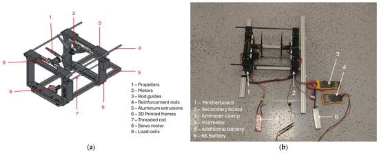
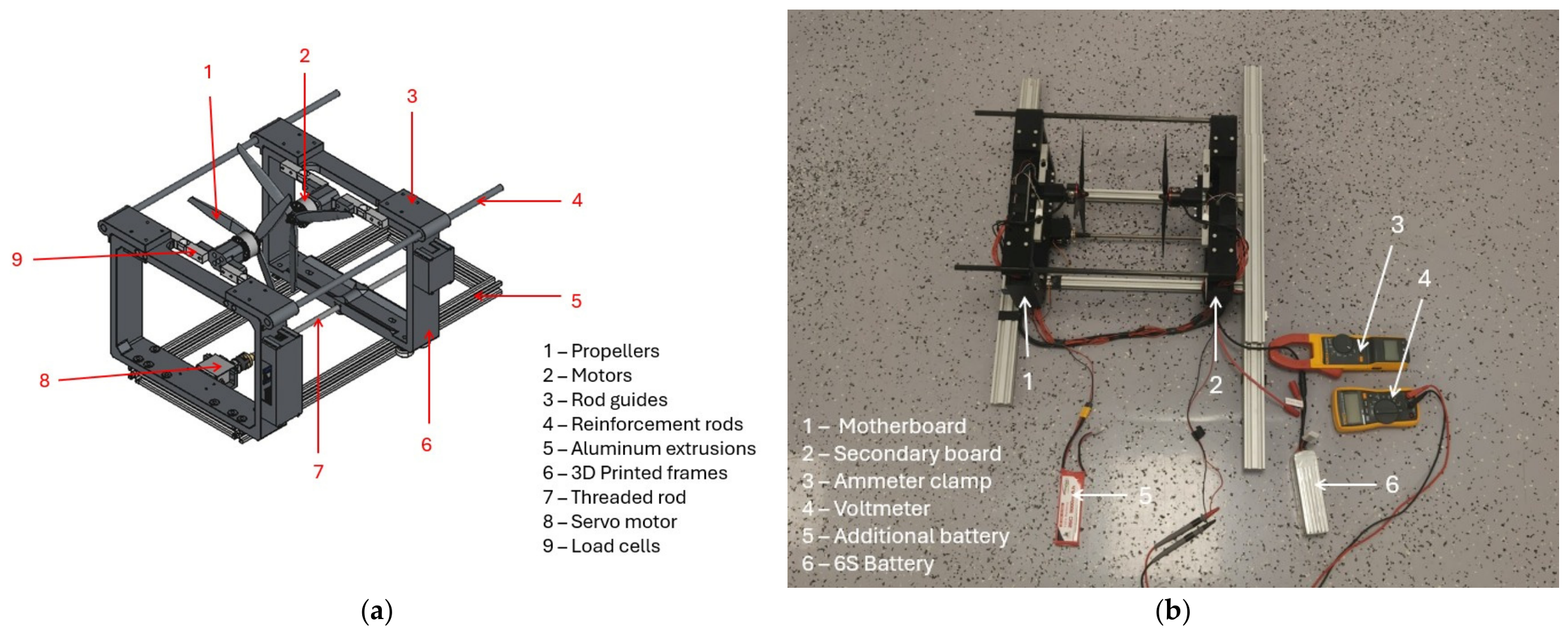
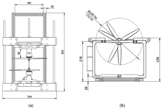
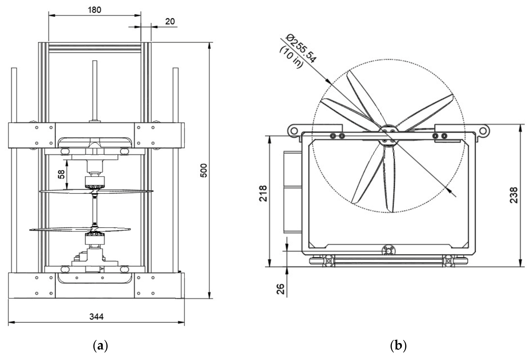
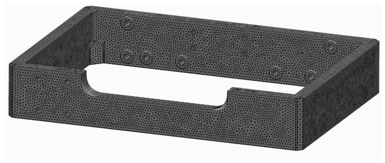
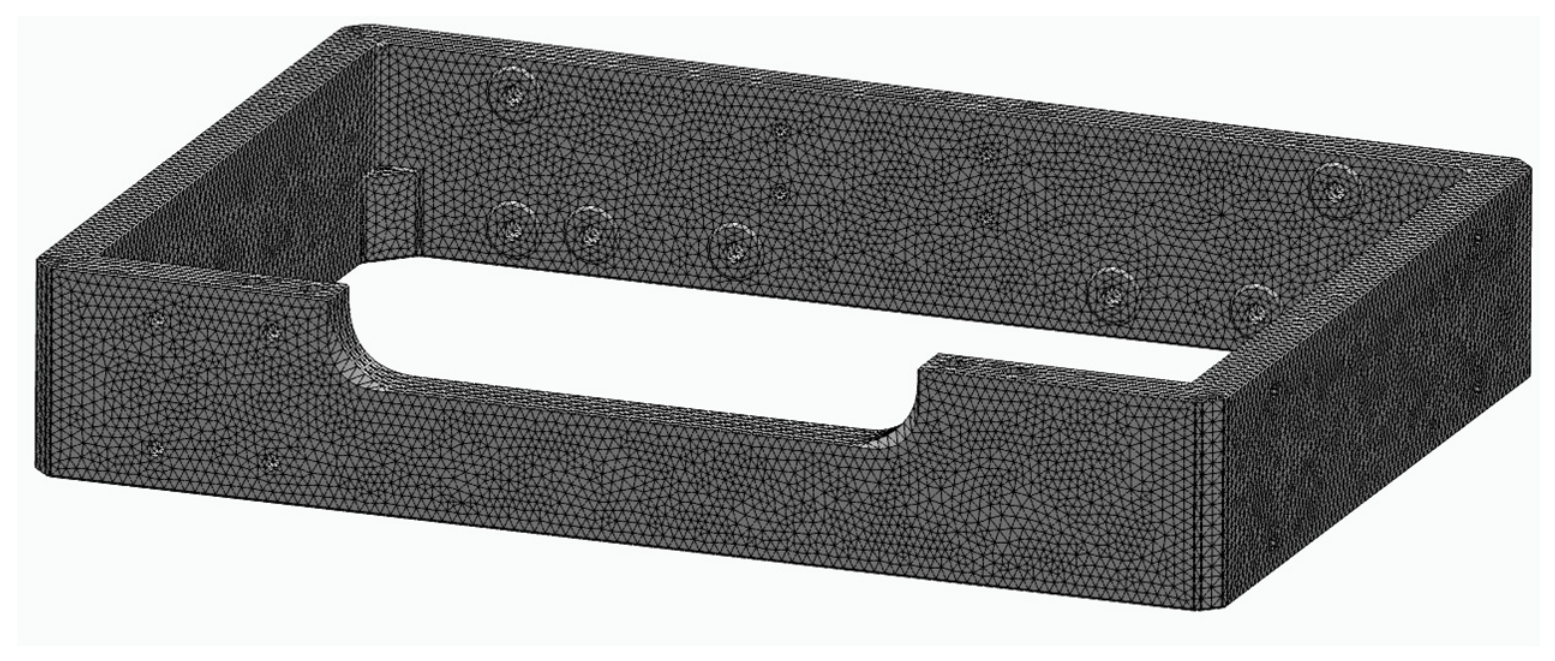
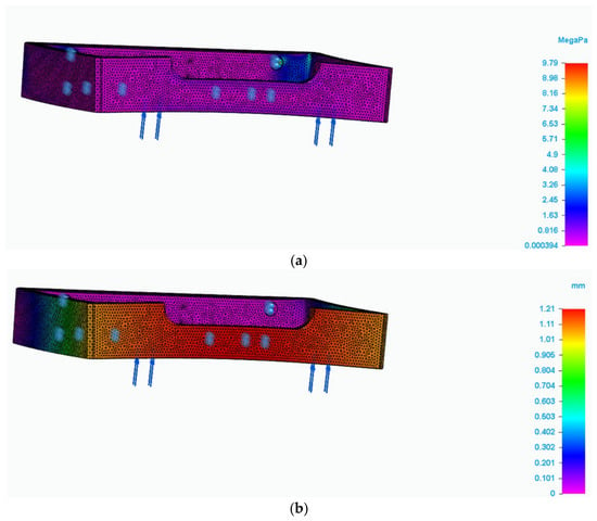
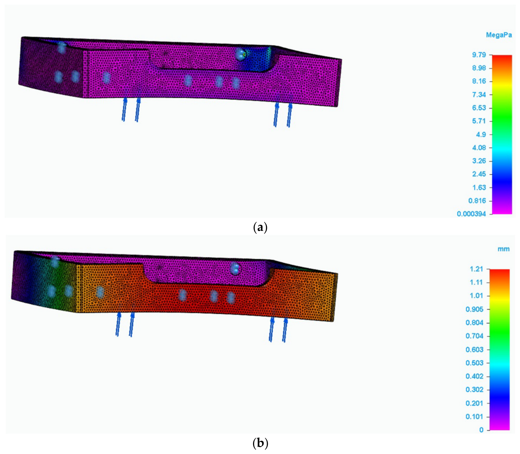
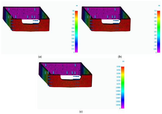
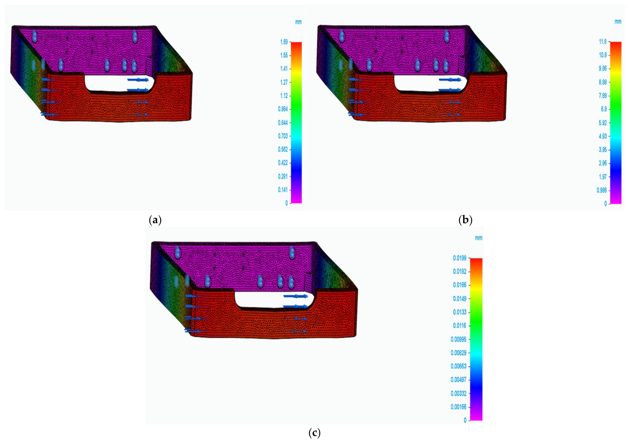
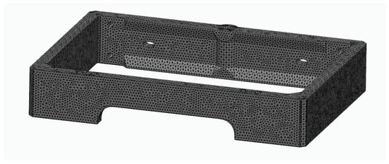
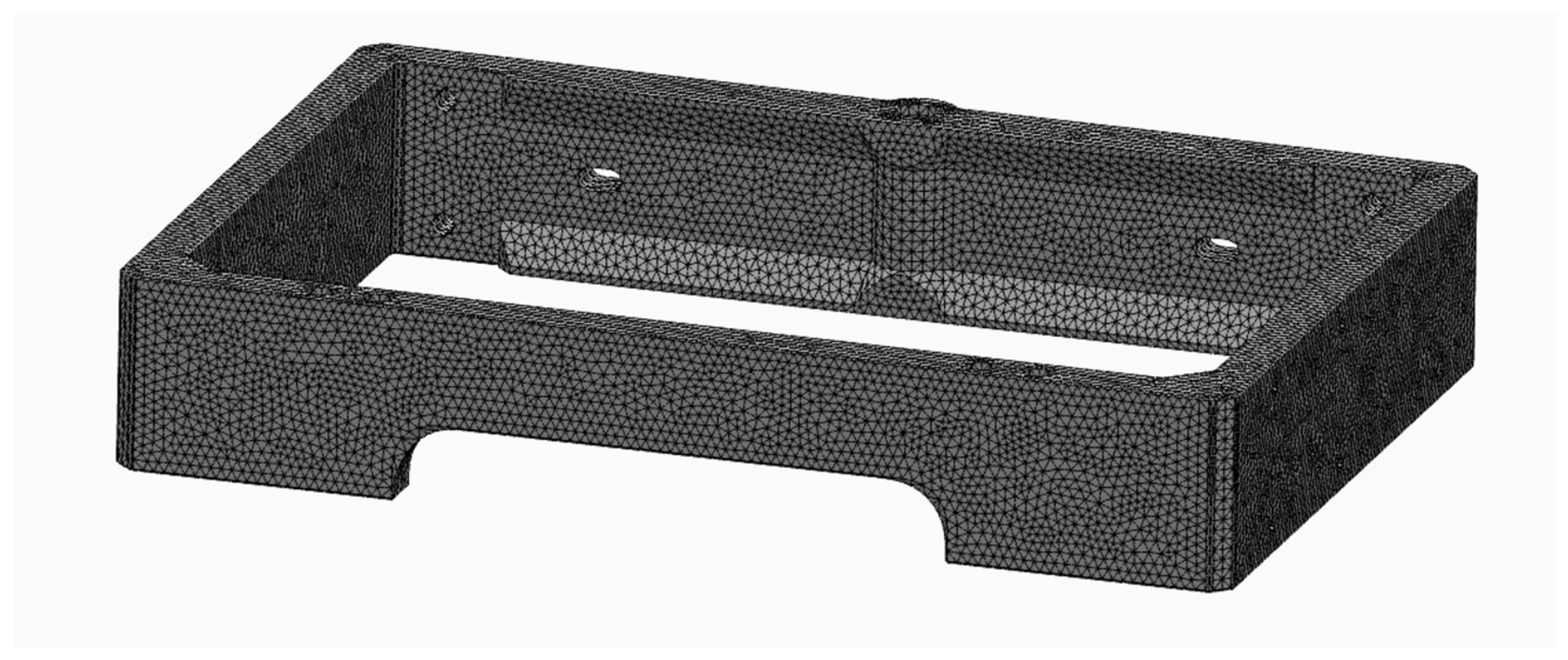
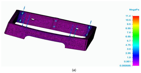
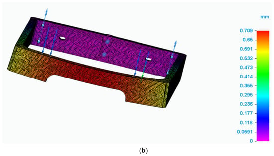
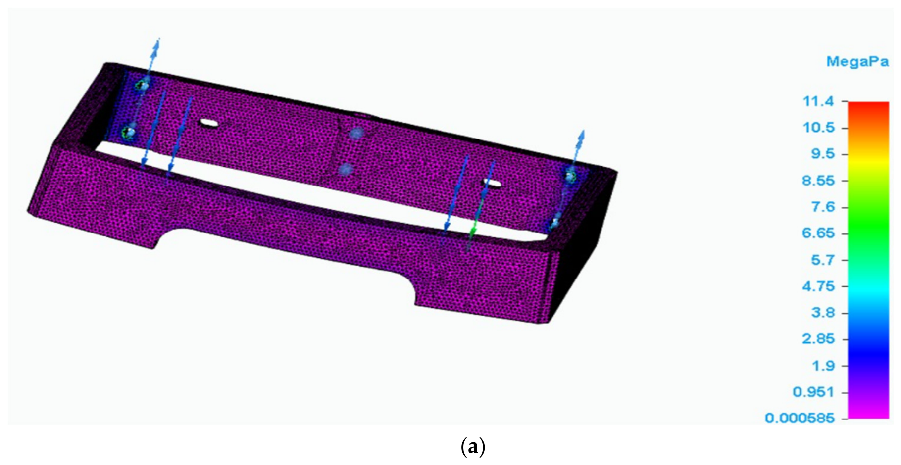
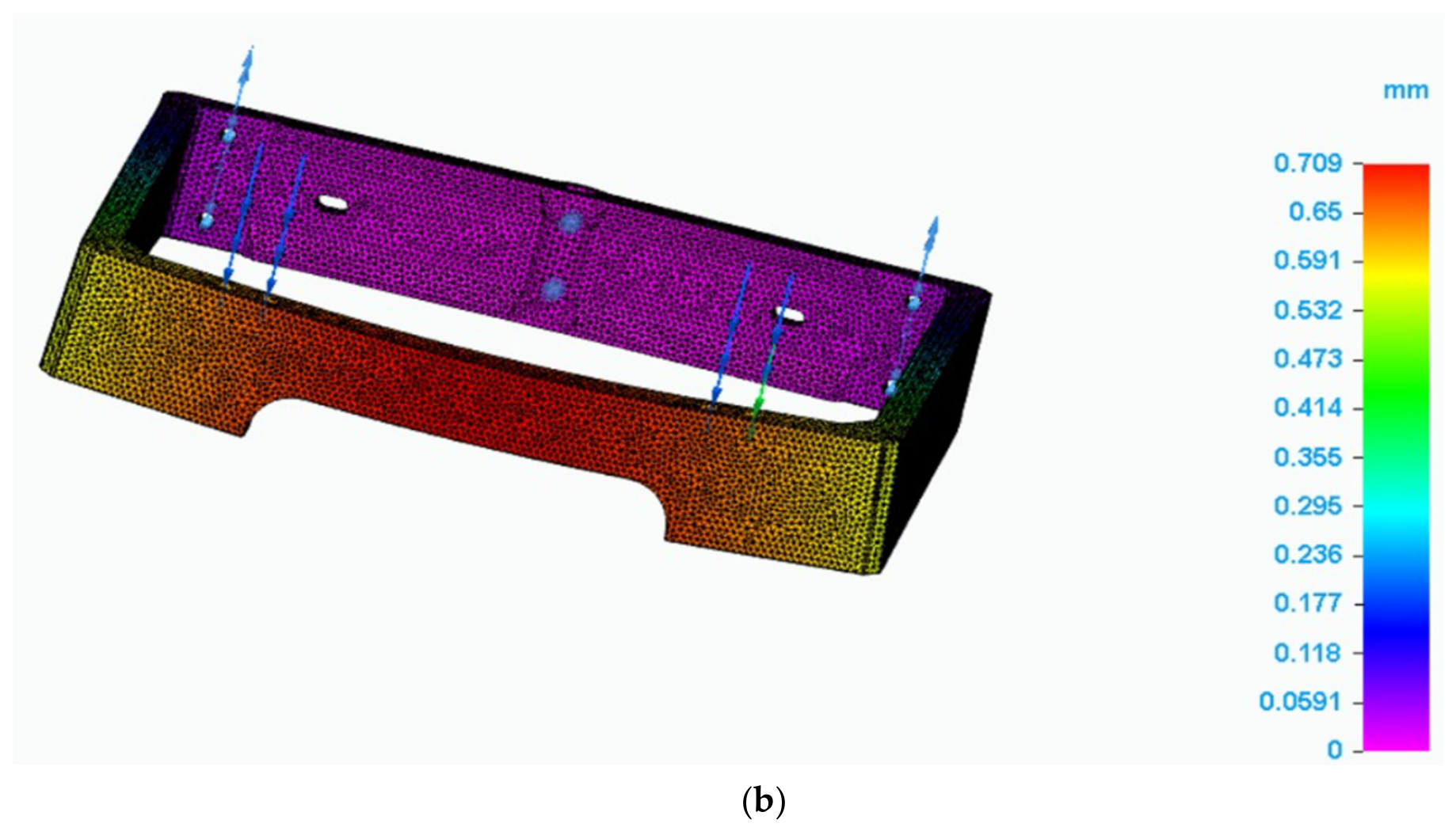
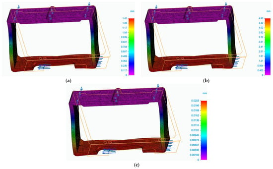
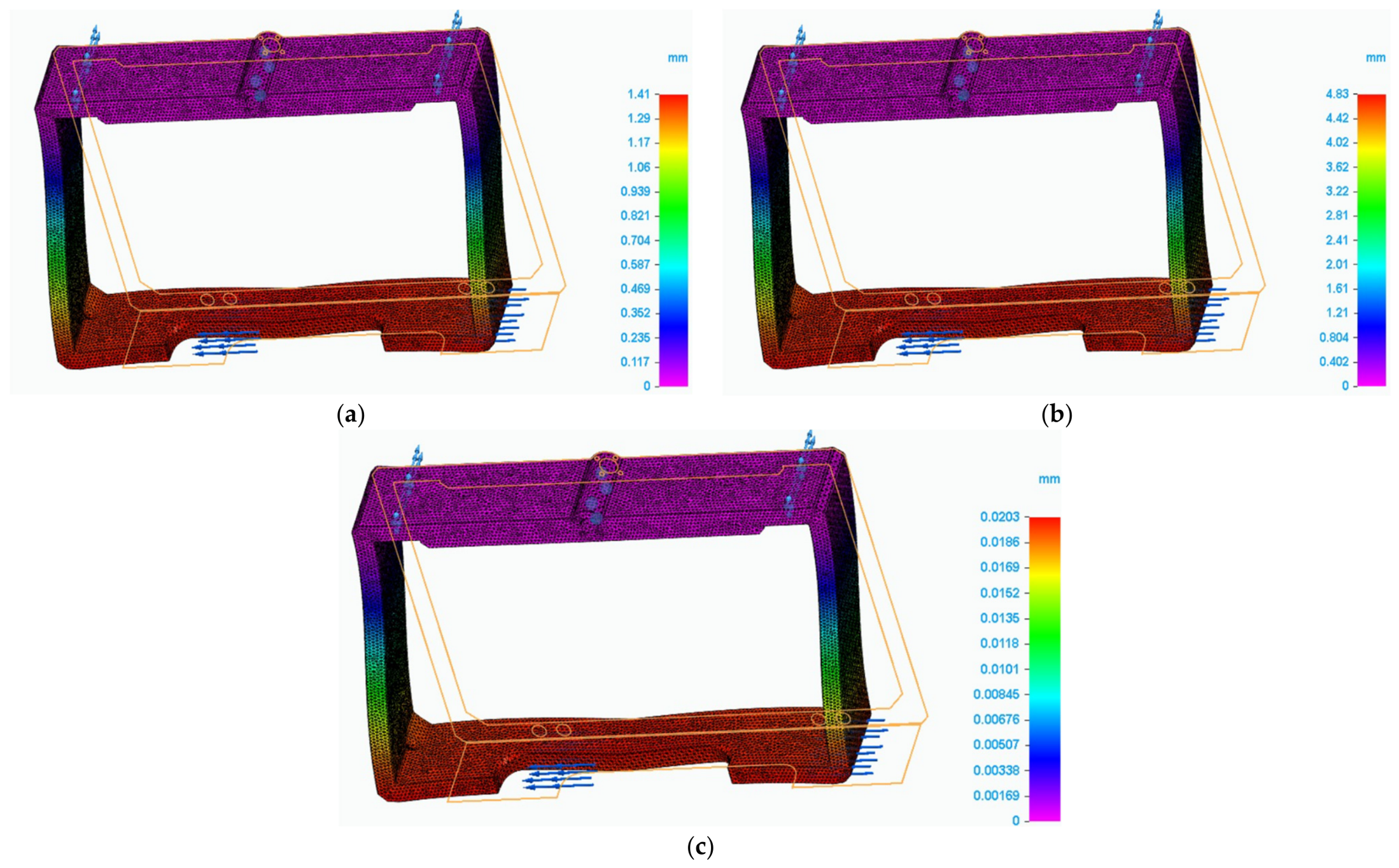
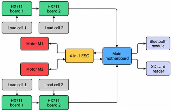
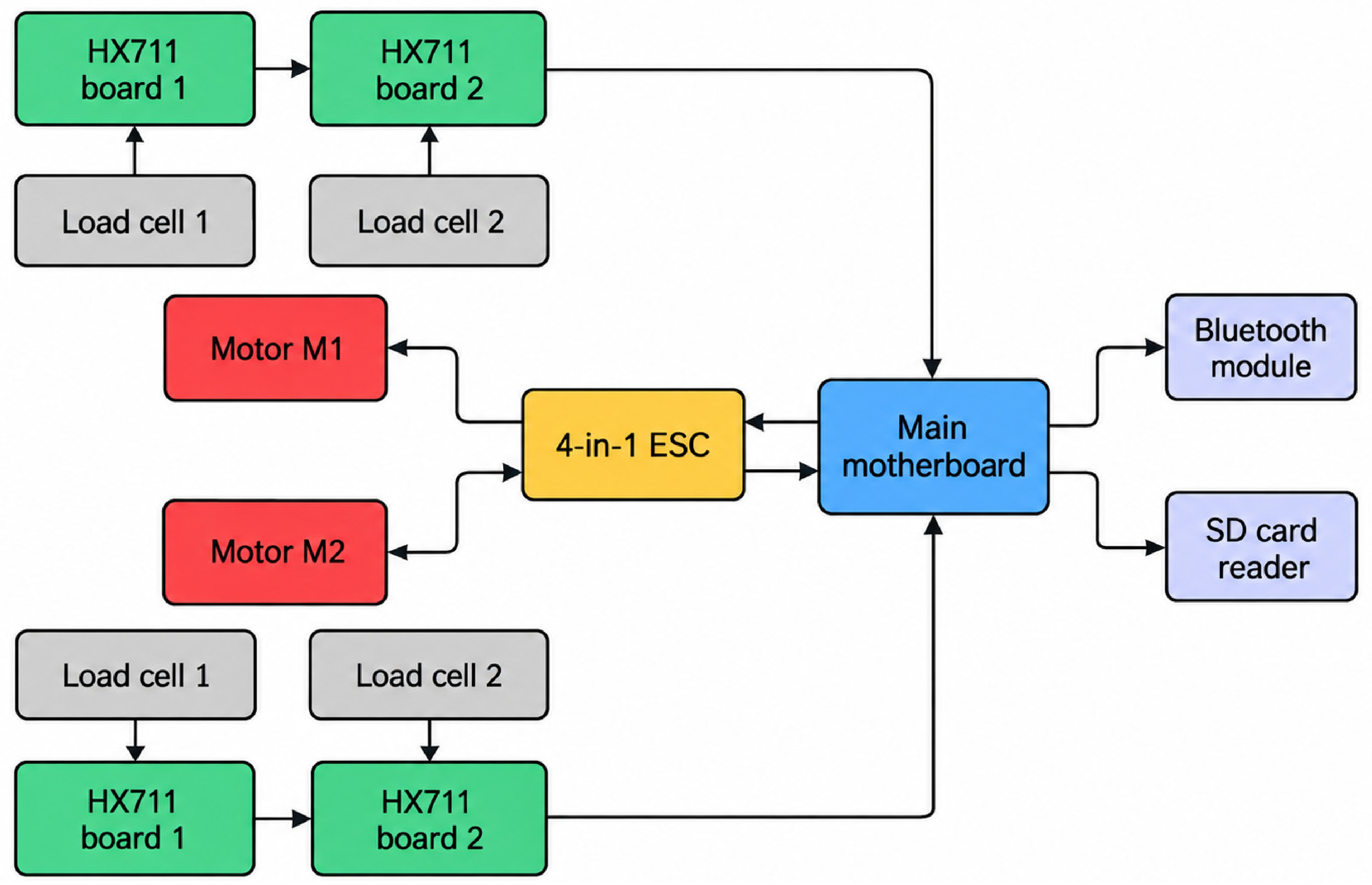
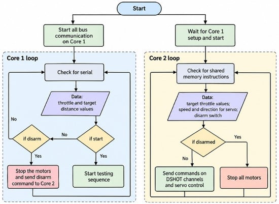
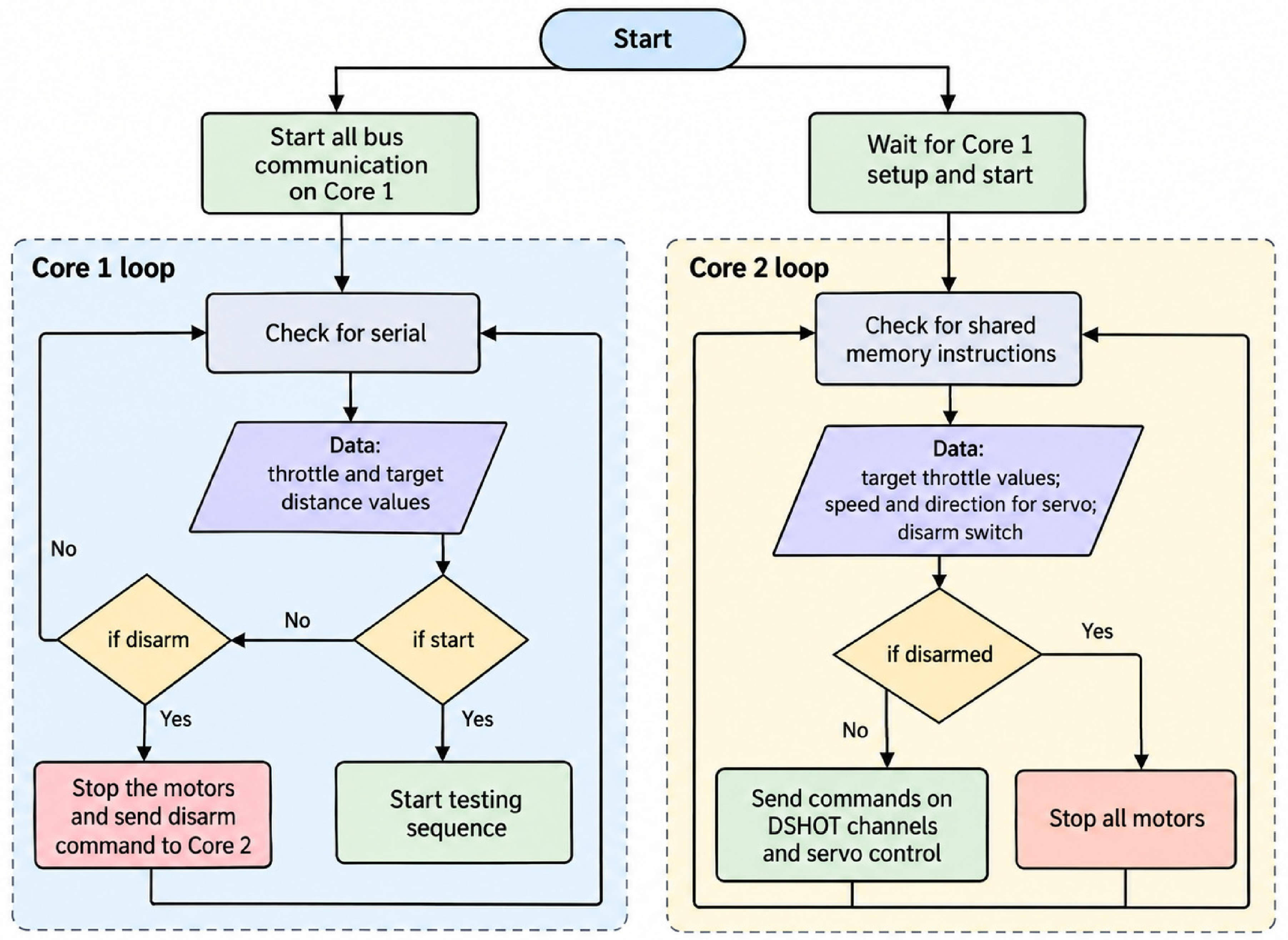
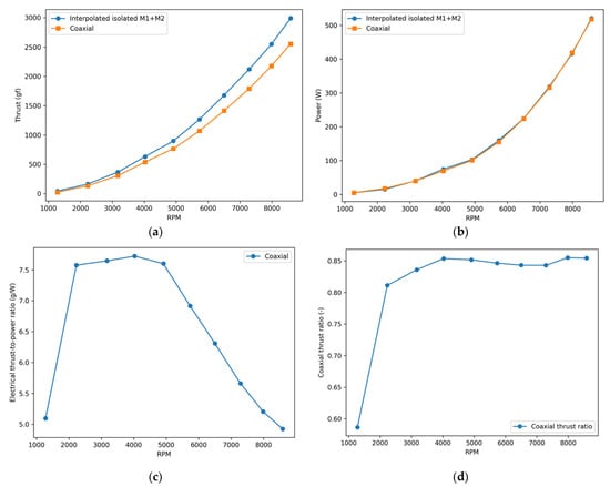
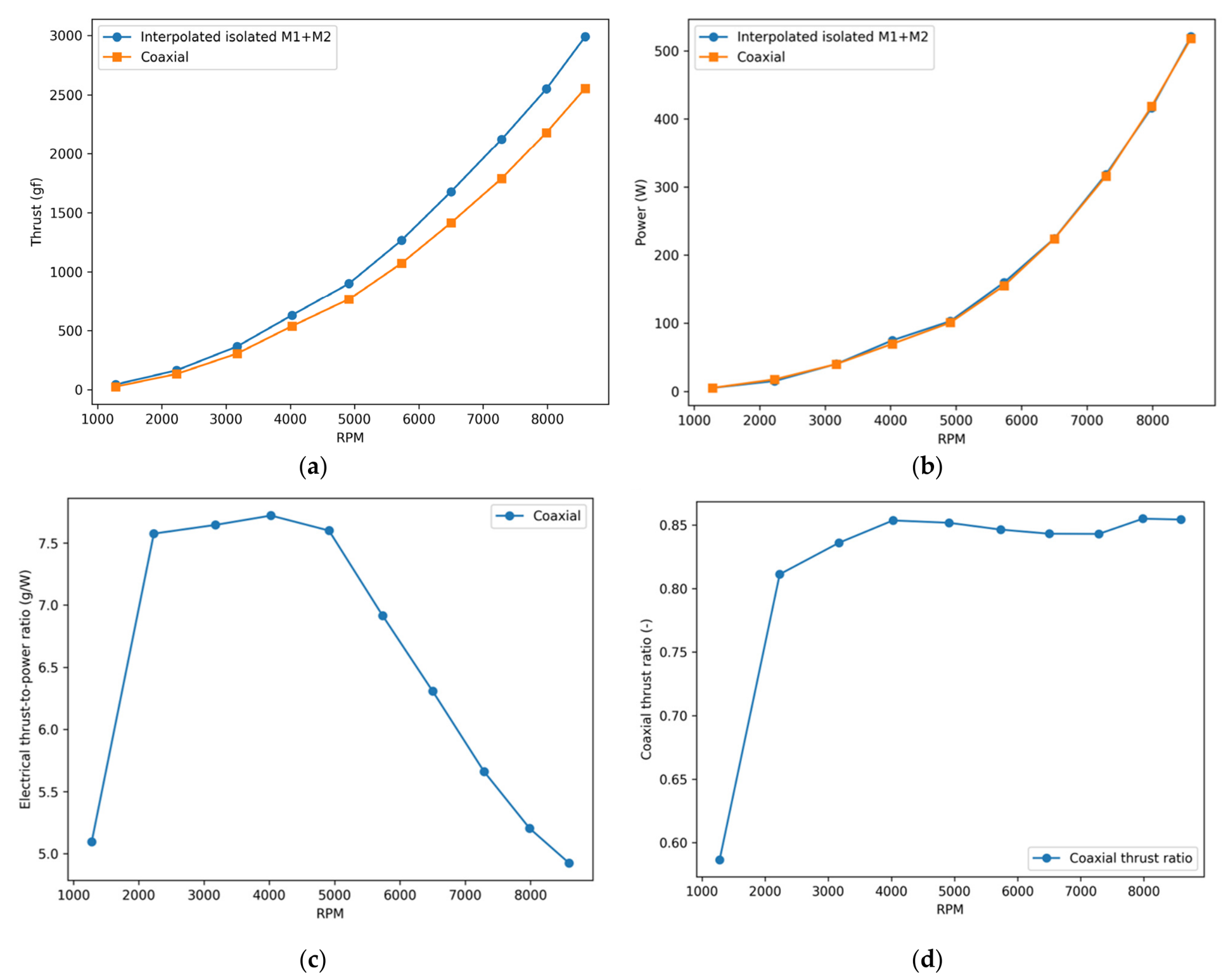
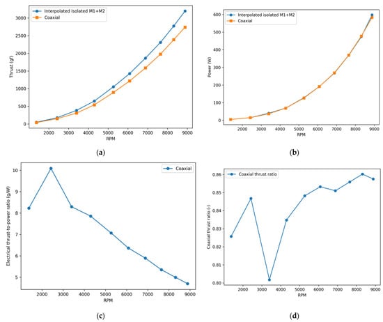
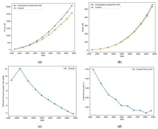
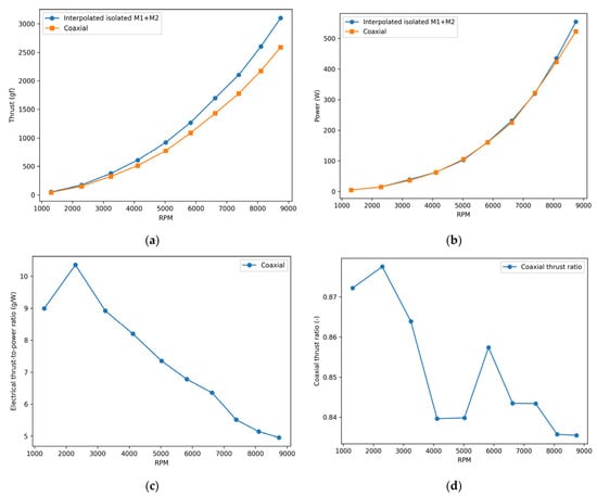
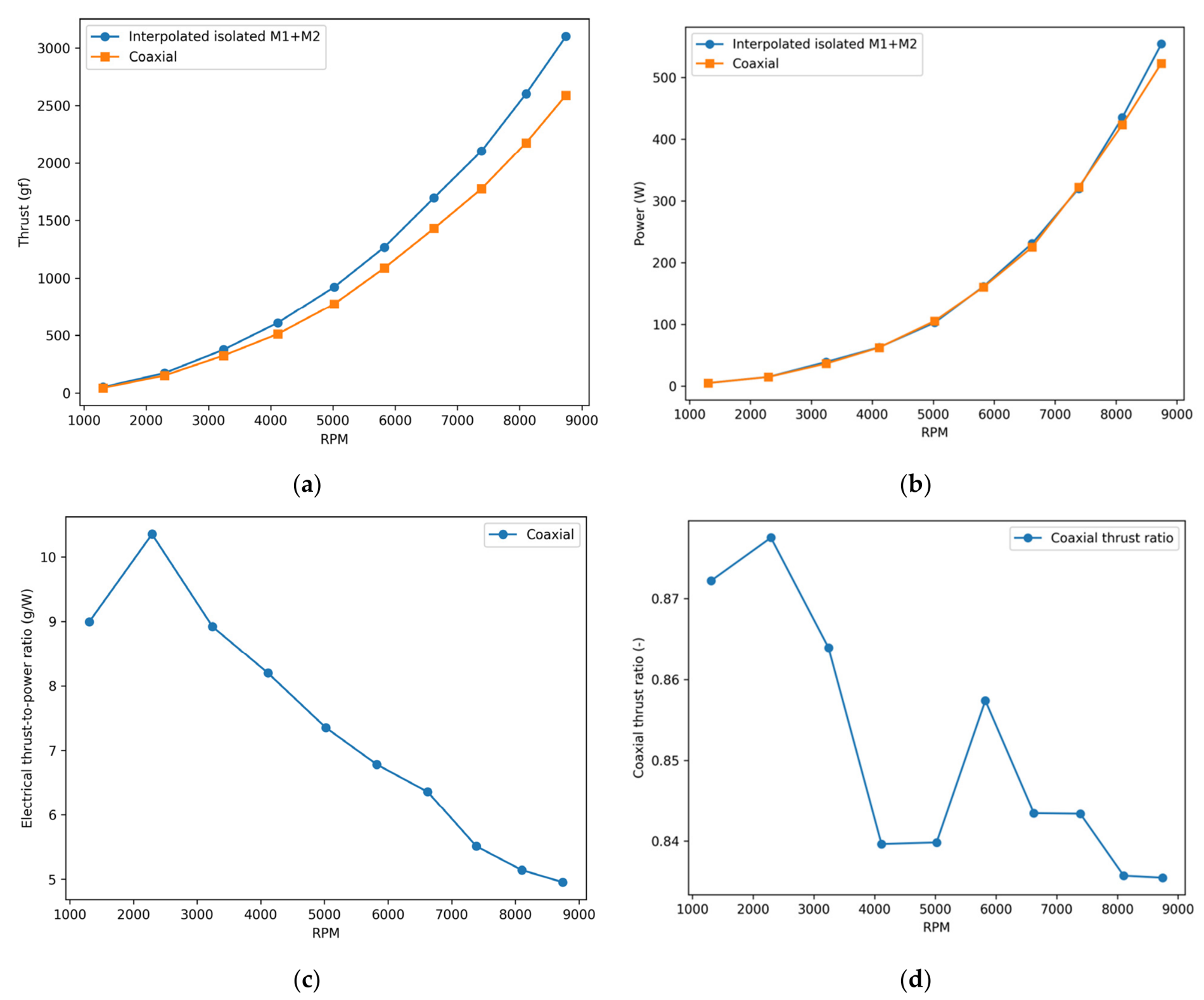
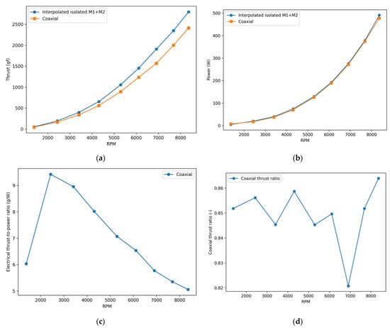
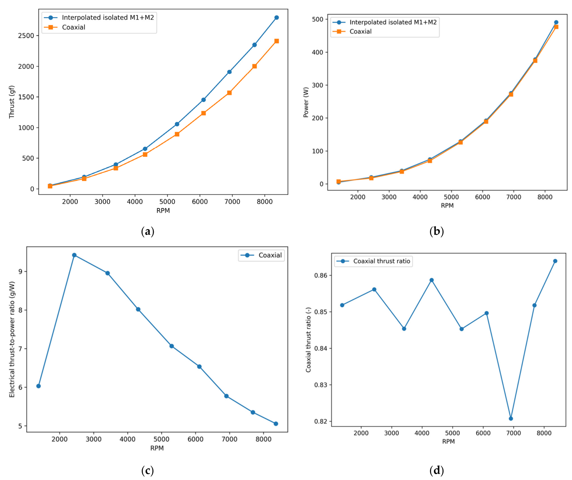
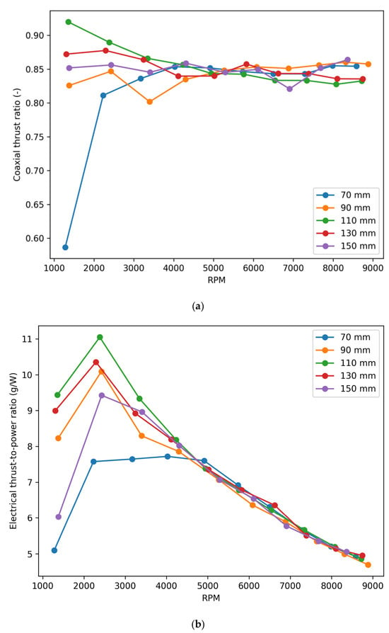
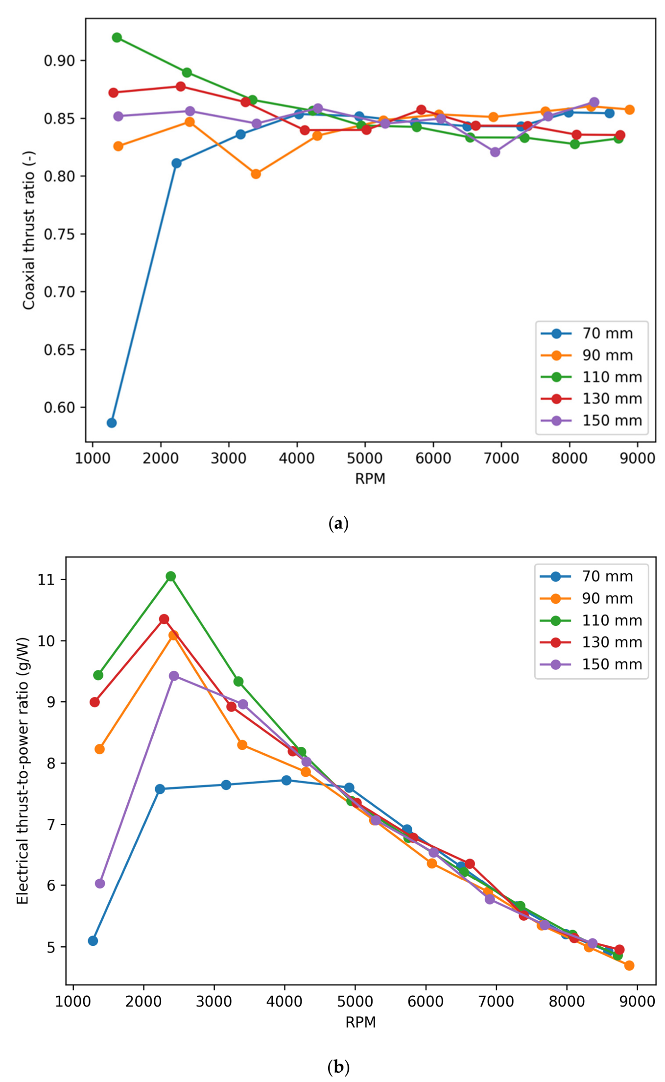
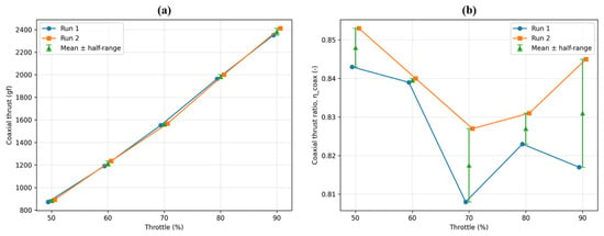
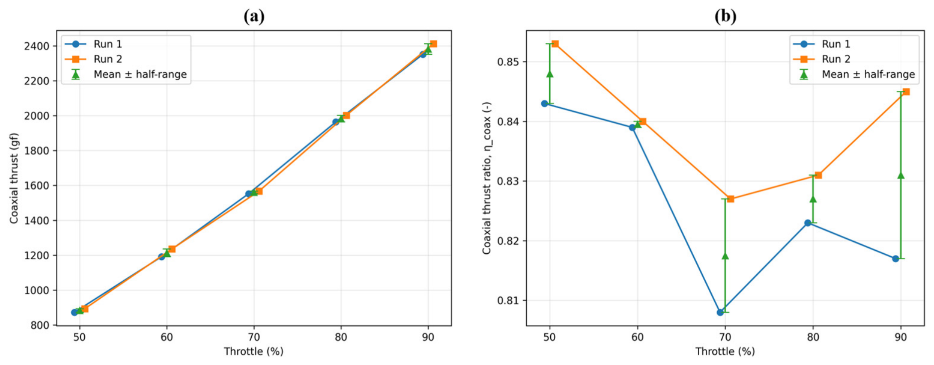
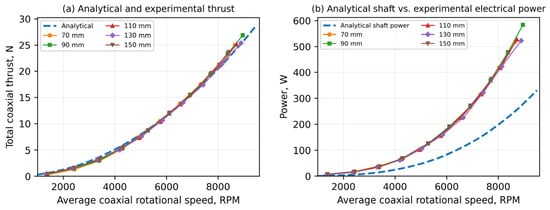
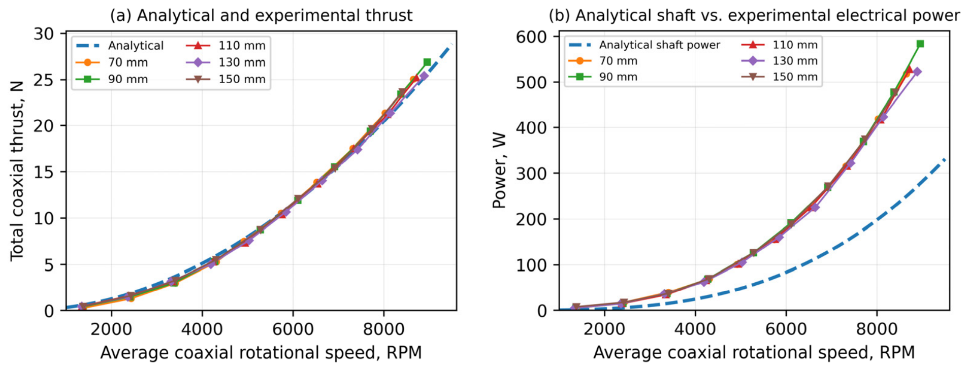
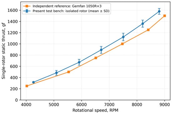
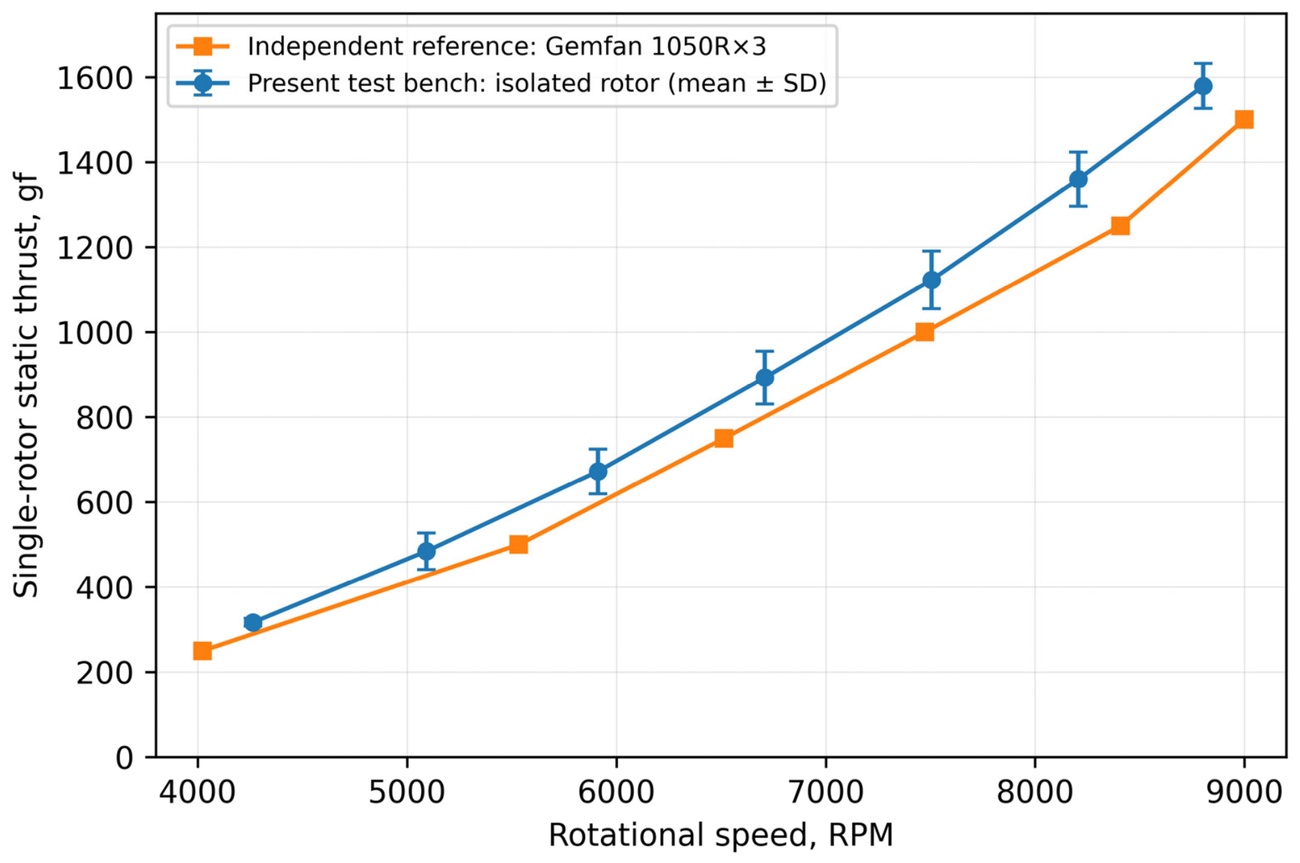

Disclaimer/Publisher’s Note: The statements, opinions and data contained in all publications are solely those of the individual author(s) and contributor(s) and not of MDPI and/or the editor(s). MDPI and/or the editor(s) disclaim responsibility for any injury to people or property resulting from any ideas, methods, instructions or products referred to in the content. |
© 2026 by the authors. Licensee MDPI, Basel, Switzerland. This article is an open access article distributed under the terms and conditions of the Creative Commons Attribution (CC BY) license.