Actuation-Aware Reference Reshaping with Adaptive Super-Twisting Tracking for Heterogeneous UAV Formations During Obstacle-Induced Maneuvers

Abstract

Heterogeneous unmanned aerial vehicle (UAV) formations face competing tracking and coordination demands during obstacle-induced maneuvers with follower-specific acceleration limits. Formation-reshaping adaptive super-twisting control (FR-ASTWC) is developed using a leader–neighbor deformation cue to drive an anchored, acceleration-limited reference before a common tracking loop. Under identical plants and tuning, FR-ASTWC is compared with direct adaptive super-twisting control (D-ASTWC), coordination-input ASTWC (C-ASTWC), and coordination-filtered-input ASTWC (CF-ASTWC). For the nominal exact drag model, ideal D-ASTWC and FR-ASTWC retain the exogenous inner residual and satisfy a verified common quadratic certificate; C-ASTWC and CF-ASTWC are empirical ablations because their residual contains the cue. At 70% capability, FR-ASTWC reduces active peak deformation, mean deformation, and plant saturation exposure relative to CF-ASTWC by 64.9%, 48.2%, and 50.8%, respectively. Across two bypass directions and three disturbance-phase variants, the mean reductions are 59.3%, 45.0%, and 47.2%. A further 1200 simulations use 100 paired uncertainty draws at each capability level. At 70%, the mean paired reductions relative to CF-ASTWC are 53.8%, 43.4%, and 46.7% for the same three metrics. Parameter sweeps and the 85% and 100% cases expose reference return and low-demand trade-offs. The evidence therefore supports a conditional architectural advantage under active heterogeneous constraints, not universal superiority or a collision avoidance guarantee.

1. Introduction

Cooperative unmanned aerial vehicles can enlarge sensing coverage, distribute payloads, and execute missions that are difficult for a single platform. Their usefulness depends not only on reaching a destination but also on maintaining a prescribed geometry while the vehicles turn, accelerate, avoid obstacles, and operate with unequal physical capabilities. Graph-based consensus and leader–follower methods provide a standard language for such coordination [1,2,3,4], while recent reviews summarize the continuing challenges of scalable UAV swarm formation control [5]. A mission-driven review published in 2026 further organized formation control around assembly, maintenance, and reconfiguration phases and highlighted resilience and heterogeneity as continuing research priorities [6]. Recent consensus research also addresses asynchronous cooperation–competition networks and bipartite agreement over quasi-structurally balanced signed networks [7,8]. These communication and interaction models broaden the coordination literature; the present study instead holds a cooperative, nonnegative, undirected graph fixed to isolate control signal placement. In a leader–follower formation, each follower may regulate a leader-relative offset and one or more neighbor-relative offsets, so local measurements are sufficient when the interaction graph is suitably connected and pinned to the leader.

UAV formation control has progressed from nominal consensus designs to time-varying formations, uncertain dynamics, communication delays, input constraints, and disturbance rejection. Dong et al. established time-varying formation conditions for UAV swarms [9]; Liang et al. addressed motion constraints and unknown disturbances in fixed-wing leader–follower formations [10]; Liu et al. and Zhou and Chen addressed input saturation [11,12]; Liu et al. examined communication delays [13]; and Yang et al. considered heterogeneous uncertainties over directed graphs [14]. A recent consensus-based study extended formation coordination to heterogeneous multi-agent systems operating in complex environments [15]. Prescribed-time networked quadrotor formation control has also been developed with explicit speed and input saturation constraints [16]. Broader surveys of constrained heterogeneous multi-agent cooperation document the same interaction between agent-level heterogeneity, network constraints, and anti-disturbance design [17], while recent fixed-time heterogeneous formation work treats multiple constraints explicitly [18]. These works demonstrate that heterogeneity and input constraints cannot be treated as secondary details. When the follower masses, normalized drag, and acceleration limits differ, the same leader maneuver does not consume the same fraction of available control capability at every vehicle.

Robust inner-loop tracking is frequently supplied by sliding-mode or higher-order sliding-mode control. The super-twisting algorithm provides continuous control action for systems with matched Lipschitz perturbations and admits strict Lyapunov analysis [19,20,21]. Adaptive gain formulations reduce the dependence on a precisely known perturbation bound [22,23]. Recent UAV studies have combined super-twisting-type controllers with formation tracking and disturbance estimation [24,25]. These developments motivate the robust tracker used here, but adaptive super-twisting control itself is not claimed as a new contribution.

A different area of the literature modifies a commanded reference before it reaches a pre-stabilized plant. Reference and command governors form a mature constraint management family in which a supervisory layer modifies commands to preserve state and input admissibility [26]. Distributed explicit reference governors and invariant-set governors have been applied to multi-UAV systems subject to thrust, velocity, collision, and workspace constraints [27,28]. Command-filtered backstepping also uses dynamic filters, principally to avoid repeated virtual control differentiation and to compensate for filter errors in strict-feedback designs [29]. The present method is neither a reference governor nor a command-filtered backstepping construction: it provides no invariant-set admissibility guarantee, and its second-order states deliberately reshape a formation target rather than approximating a virtual control derivative. Its nearest architectural question is whether excessive coordination demand should be handled upstream in the commanded trajectory or injected into the limited plant channel.

Obstacle-rich UAV missions add another layer to this question. Trajectory generation methods can provide dynamically smooth, collision-free paths for individual quadrotors and large swarms [30,31]. Formation control studies have also integrated artificial potential field or optimal consensus methods with obstacle avoidance [32,33]. A recent bearing-based distributed design combined single-leader formation tracking with obstacle avoidance behavior [34]. In this paper, obstacle avoidance is not redesigned. A common, smooth bypass trajectory is supplied by an external mission planner to all compared controllers. The control question is narrower: how should heterogeneous followers maintain formation while executing a demanding maneuver with limited translational actuation capability?

Most distributed formation controllers place leader–neighbor correction directly in the control input. Under generous input capability, this is natural and effective. Under tight limits, however, leader feedforward, drag compensation, robust tracking, and coordination all compete in the same saturated channel. Feng et al. replace a nominal deadline-guided performance boundary with an executable boundary computed from online maneuvering capability for fixed-wing formation tracking with nonholonomic coupling [35]. FR-ASTWC operates at a different layer: it reshapes the tracked translational follower reference so that the coordination cue is absent from the inner sliding-mode residual. Merely increasing coordination or sliding gains cannot increase the physical acceleration available to the follower. This motivates an actuation-aware decomposition in which deformation first reshapes an anchored, acceleration-limited follower reference and a common robust controller subsequently tracks it.

Table 1 distinguishes the mechanism investigated here from neighboring approaches. The contribution is a controlled comparison of where a local deformation cue enters an otherwise shared tracker, together with the resulting residual identity. Neither command modification nor adaptive super-twisting control is claimed to be new in isolation. The study does not benchmark external methods or transfer their admissibility and safety guarantees to FR-ASTWC.

Table 1. Position of the proposed architecture relative to related control approaches.

Approach	Principal Mechanism	Distinction from This Study
Reference governors [26,28]	Modify commands using admissibility or invariant-set information.	FR uses a local deformation-driven dynamic reference and radial acceleration limit, without invariant-set constraint enforcement.
Command-filtered backstepping [29]	Filter virtual controls and compensate filter error in a recursive design.	FR changes the physical tracking target of a common STA loop; CF is an input placement ablation, not a backstepping design.
Capability-aware formation tracking [35]	Adjust an executable performance boundary using available maneuvering capability.	FR reshapes follower position/velocity references; no deadline boundary or predictive coordination layer is used.
FR-ASTWC	Compare direct, filtered input, and reference placement under identical plant limits and inner-loop settings.	Ideal residual separation is established; constrained performance is evaluated numerically and remains conditional.

This paper makes the following contributions.

• A formation deformation-driven reference layer is developed for heterogeneous leader–follower UAVs. The local pinned neighborhood deformation and its rate modify a dynamically anchored follower trajectory, and a separate radial limit is applied to the reference acceleration before the robust inner loop acts.
• A four-way controlled placement study compares direct adaptive super-twisting control (D-ASTWC), coordination-input ASTWC (C-ASTWC), coordination-filtered-input ASTWC (CF-ASTWC), and formation-reshaping ASTWC (FR-ASTWC). D-ASTWC contains no explicit deformation correction; C-ASTWC injects the cue directly; CF-ASTWC dynamically filters the cue but still injects it at the plant input; and FR-ASTWC tracks states generated by the same filter law. Thus, C versus CF isolates filtering, whereas CF versus FR isolates reference versus input placement. Separate closed-loop runs need not have identical filter state histories.
• The pinned graph identity relates local deformation to global formation error. The ideal super-twisting certificate is stated only for D-ASTWC and FR-ASTWC, whose inner residual remains the matched exogenous term. The larger, state-dependent residual slopes of C-ASTWC and CF-ASTWC are disclosed a posteriori rather than folded into a circular common proof.
• A smooth obstacle bypass maneuver is evaluated at 100%, 85%, and 70% follower capability. The 85% case is explicitly identified as plant-kinematically feasible but marginal, and the 70% case is repeated for two bypass directions and three disturbance phases. A 144-run local parameter sweep and a 1200-run paired Monte Carlo study assess tuning sensitivity and a declared joint-uncertainty family without retuning the inner tracker.

In this paper, actuation-aware means that the upstream reference generator explicitly applies each follower’s acceleration limit $a_{r,i,\max }$; it does not mean that the controller creates additional physical actuation or decision authority.

The remainder of the paper is organized as follows. Section 2 defines the heterogeneous mass-normalized model and pinned graph. Section 3 introduces the formation errors and placement objective. Section 4 presents the common module and four placements. Section 5 separates the D/FR certificate from conditional practical bounds and C/CF diagnostics. Section 6 defines the complete numerical protocol. Section 7 and Section 8 report and interpret the results, and Section 9 concludes the paper.

2. Heterogeneous UAV Model and Graph Preliminaries

Throughout, $∥·∥$ denotes the Euclidean vector norm or induced matrix 2-norm; ${∥·∥}_F$ and ${∥·∥}_{\infty }$ denote the Frobenius and infinity norms. The operators col, ⊗, and $I_n$ denote column stacking, the Kronecker product, and the n-dimensional identity, respectively. An identity without a subscript has the dimension required by its equation.

Consider one leader and N follower UAVs. The follower set is

$${𝒱}_f=\{1,2,\dots ,N\},$$

(1)

and the leader is indexed by L. The position and velocity of follower i in an inertial frame are $p_i,v_i\in {\mathbb{R}}^3$; the leader variables are $p_L,v_L\in {\mathbb{R}}^3$, with $a_L={\dot{v}}_L$.

The fixed follower information topology is the undirected weighted graph

$${\mathcal{G}}_f=({𝒱}_f,{\mathcal{E}}_f,A),$$

(2)

where ${\mathcal{E}}_f$ is the set of undirected communication edges between followers, and $A=\left[a_{ij}\right]=A^{\top }\ge 0$ is the weighted adjacency matrix, with $a_{ij}>0$ if and only if $\{i,j\}\in {\mathcal{E}}_f$ for $i\ne j$, and $a_{ii}=0$. The neighbor set and degree of follower i are

$${\mathcal{N}}_i=\{j\in {𝒱}_f\backslash \left\{i\right\}:\{i,j\}\in {\mathcal{E}}_f\},q_i=\left|{\mathcal{N}}_i\right|.$$

(3)

The leader’s influence on each follower $i\in {𝒱}_f$ is represented by the pinning weight $a_{iL}\ge 0$. The leader is not included in the follower-neighbor set ${\mathcal{N}}_i$.

2.1. Physical and Mass-Normalized Translational Models

The physical translational model is

$${\dot{p}}_i=v_i,m_i{\dot{v}}_i=F_i-D_i{v}_i+d_i^F\left(t\right)+{\varphi }_i^F(p_i,v_i,t),$$

(4)

where $m_i>0$ is the mass, $F_i\in {\mathbb{R}}^3$ is the commanded translational force, $D_i=D_i^{\mathsf{T}}⪰0$ is the physical drag coefficient matrix, $d_i^F$ is an external force disturbance, and ${\varphi }_i^F$ collects matched aerodynamic and low-level model residuals. The actual drag force is $-D_i{v}_i$.

Define

$$u_i={\displaystyle \frac{F_i}{m_i}},{\mathsf{B}}_i={\displaystyle \frac{D_i}{m_i}},{\omega }_i={\displaystyle \frac{d_i^F+{\varphi }_i^F}{m_i}}.$$

(5)

Then,

$${\dot{p}}_i=v_i,{\dot{v}}_i=u_i-{\mathsf{B}}_i{v}_i+{\omega }_i\left(t\right).$$

(6)

Here, $-{\mathsf{B}}_i{v}_i$ is the normalized drag acceleration. For the isotropic translational drag model used in the simulations, ${\mathsf{B}}_i={\beta }_i{I}_3$ with follower-dependent ${\beta }_i$. The simulated plant is propagated entirely in mass-normalized acceleration coordinates; once ${\mathsf{B}}_i$ and $a_{i,\max }$ are specified, the tabulated $m_i$ is used only to recover physical drag and force quantities and does not independently alter the trajectories.

Let ${\widehat{\mathsf{B}}}_i$ be the normalized drag matrix used by the controller and define the matched residual

$${\vartheta }_i={\omega }_i+({\widehat{\mathsf{B}}}_i-{\mathsf{B}}_i)v_i.$$

(7)

The controller-oriented plant is

$${\dot{p}}_i=v_i,{\dot{v}}_i=u_i-{\widehat{\mathsf{B}}}_i{v}_i+{\vartheta }_i.$$

(8)

The nominal capability sweep, six-scenario ensemble, and design parameter sensitivity study use ${\widehat{\mathsf{B}}}_i={\mathsf{B}}_i$, so ${\vartheta }_i={\omega }_i$. The additional Monte Carlo study in Section 6.7 varies the true drag while retaining the nominal controller estimate. In these runs, the residual includes the velocity-dependent mismatch term in (7), and the nominal certificate is not asserted. Unknown mass is not tested.

The unsaturated acceleration-like command $u_i^{\star }$ is implemented through radial saturation,

$$u_i={\mathrm{sat}}_{a_{i,\max }}\left(u_i^{\star }\right),$$

(9)

where

$${\mathrm{sat}}_{\overline{a}}\left(\xi \right)=\left\{\begin{array}{cc}\xi ,\hfill & ∥\xi ∥\le \overline{a},\hfill \\ \overline{a}\xi /∥\xi ∥,\hfill & ∥\xi ∥>\overline{a}.\hfill \end{array}\right.$$

(10)

The available translational actuation capability is therefore the set

$${\mathcal{U}}_i=\{u_i\in {\mathbb{R}}^3:∥u_i∥\le a_{i,\max }\}.$$

(11)

Define the plant saturation residual

$${\epsilon }_{a,i}=u_i-u_i^{\star }.$$

(12)

Then,

$${\dot{v}}_i=u_i^{\star }-{\widehat{\mathsf{B}}}_i{v}_i+{\vartheta }_i+{\epsilon }_{a,i}.$$

(13)

Assumption 1

(Leader regularity). The leader trajectory is twice locally absolutely continuous, and $v_L,a_L\in L_{\infty }$, i.e., the leader velocity and acceleration are essentially bounded. The desired follower offsets are constant.

Assumption 2

(Matched residual). Each ${\vartheta }_i$ is absolutely continuous, with

$$∥{\vartheta }_i\left(t\right)∥\le {\overline{\vartheta }}_i,∥{\dot{\vartheta }}_i\left(t\right)∥\le {\overline{\ell }}_i.$$

(14)

Here, ${\overline{\vartheta }}_i$ and ${\overline{\ell }}_i$ are finite nonnegative constants bounding the matched-residual magnitude and its time derivative magnitude, respectively.

Assumption 3

(Local information). Follower i has access to its own position and velocity; the leader-relative state, relative position, and velocity with respect to each $j\in {\mathcal{N}}_i$; and the planner broadcast $a_L$. The broadcast is required even for a follower whose pinning coefficient is zero: pinning specifies formation error coupling, whereas $a_L$ is common trajectory feedforward. The present study assumes a fixed graph and does not model communication delay or packet loss.

2.2. Pinned Interaction Matrix

Define the follower Laplacian and leader-pinning matrix

$$L_a=D_a-A,D_a=\mathrm{diag}\left(\sum _j{a}_{1j},\dots ,\sum _j{a}_{Nj}\right),$$

(15)

$$G_L=\mathrm{diag}(a_{1L},\dots ,a_{NL}),$$

(16)

and the pinned matrix

$$H=L_a+G_L.$$

(17)

Assumption 4

(Pinned, row-normalized graph). The follower graph is fixed, undirected, and connected, and at least one follower has a positive leader-pinning weight. The cue weights obey

$$a_{iL}+\sum _{j\in {\mathcal{N}}_i}{a}_{ij}=1.$$

(18)

Consequently, $H=H^{\mathsf{T}}\succ 0$; for this convention, $H=I_N-A$ when A contains only follower–follower weights.

Indeed,

$$y^{\mathsf{T}}Hy={\displaystyle \frac{1}{2}}{\displaystyle \sum _{i=1}^N}{\displaystyle \sum _{j=1}^N}{a}_{ij}{(y_i-y_j)}^2+{\displaystyle \sum _{i=1}^N}{a}_{iL}{y}_i^2>0$$

(19)

for every nonzero $y\in {\mathbb{R}}^N$ under Assumption 4.

3. Problem Formulation and Formation Deformation Signals

Assign follower i the constant desired leader-relative displacement $r_i\in {\mathbb{R}}^3$. The consistent desired pairwise offset is

$${\Delta }_{iL}=r_i,{\Delta }_{ij}=r_i-r_j.$$

(20)

The nominal follower reference is

$$p_{d,i}^0=p_L+r_i,v_{d,i}^0=v_L,a_{d,i}^0=a_L.$$

(21)

Define

$$e_{iL}=(p_i-p_L)-r_i,$$

(22)

$$e_{ij}=(p_i-p_j)-(r_i-r_j),j\in {\mathcal{N}}_i.$$

(23)

The local formation error matrix and its sliding matrix are

$$E_i=\left[\begin{array}{cccc}{e}_{iL}& e_{i{j}_1}& \cdots & e_{i{j}_{q_i}}\end{array}\right],$$

(24)

$$S_i={\dot{E}}_i+{\Lambda }_{f,i}{E}_i,{\Lambda }_{f,i}={\Lambda }_{f,i}^{\mathsf{T}}\succ 0.$$

(25)

The degree-normalized scalar scheduling signal is

$${\rho }_i={\displaystyle \frac{{∥S_i∥}_F}{\sqrt{q_i+1}}}.$$

(26)

It has units of velocity and is used only to schedule the common adaptive gains. The normalization avoids automatically producing larger scheduled gains at nodes with more local error columns. Graph weights are intentionally not applied in (26); they shape the coordination cue below rather than being counted twice.

Let

$$w_i={\left[\begin{array}{cccc}{a}_{iL}& a_{i{j}_1}& \cdots & a_{i{j}_{q_i}}\end{array}\right]}^{\mathsf{T}},{\dot{w}}_i=0.$$

(27)

Equation (18) gives ${\mathbf{1}}^{\mathsf{T}}{w}_i=1$. The locally computable deformation vector is

$${\chi }_i=E_i{w}_i=a_{iL}{e}_{iL}+\sum _{j\in {\mathcal{N}}_i}{a}_{ij}{e}_{ij},$$

(28)

with ${\dot{\chi }}_i={\dot{E}}_i{w}_i$.

Define

$$x_i=e_{iL},x=\mathrm{col}(x_1,\dots ,x_N),\chi =\mathrm{col}({\chi }_1,\dots ,{\chi }_N),\overline{H}=H\otimes I_3.$$

(29)

Offset consistency gives $e_{ij}=x_i-x_j$ and therefore

$$\begin{array}{|c|}\hline \chi =\overline{H}x.\\ \hline\end{array}$$

(30)

Since $H\succ 0$,

$${\lambda }_{\min }\left(H\right)∥x∥\le ∥\chi ∥\le {\lambda }_{\max }\left(H\right)∥x∥.$$

(31)

Thus, regulating the local deformation vectors bounds the global leader-relative formation error. This is a graph-based local-to-global bound, not the cooperative sharing of physical actuation capability.

The shared deformation cue is

$$g_{f,i}=K_{p,f,i}{\chi }_i+K_{d,f,i}{\dot{\chi }}_i,$$

(32)

where $K_{p,f,i},K_{d,f,i}\succ 0$. Four placements are compared under the same plant, disturbances, graph, inner robust controller parameters, initial gains, and final actuator limits.

$$\begin{array}{cc}\hfill \text{D-ASTWC}:& \mathrm{no}\mathrm{explicit}{g}_{f,i}\mathrm{in}\mathrm{the}\mathrm{nominal}\mathrm{reference}\mathrm{or}\mathrm{plant}\mathrm{command}.\hfill \\ \hfill \text{C-ASTWC}:& -g_{f,i}\mathrm{is}\mathrm{added}\mathrm{directly}\mathrm{to}\mathrm{the}\mathrm{final}\mathrm{plant}\mathrm{command}.\hfill \\ \hfill \text{CF-ASTWC}:& \mathrm{the}\mathrm{dynamically}\mathrm{filtered}\mathrm{cue}\mathrm{is}\mathrm{added}\mathrm{to}\mathrm{the}\mathrm{final}\mathrm{plant}\mathrm{command}.\hfill \\ \hfill \text{FR-ASTWC}:& -g_{f,i}\mathrm{drives}\mathrm{an}\mathrm{anchored},\mathrm{limited}\mathrm{reference}\mathrm{before}\mathrm{tracking}.\hfill \end{array}$$

(33)

D-ASTWC computes ${\rho }_i$ for the common gain scheduler but injects no additive correction (32) into either its reference or its plant command. C-ASTWC and CF-ASTWC are controlled numerical ablations. Only D-ASTWC and FR-ASTWC retain the exogenous ideal inner residual required by the formal certificate in Section 5. Table 2 summarizes these placements and their ideal inner residuals.

Table 2. Architecture comparison. Every realization uses the same deformation-based gain scheduler. Residuals are for the ideal unsaturated inner loop; the nominal exact drag case has ${\vartheta }_i={\omega }_i$.

Method	Tracked Position	Additive Cue Placement	Upstream Dynamics/Limit	Inner Residual
D	$p_{d,i}^0$	None	None	${\vartheta }_i$
C	$p_{d,i}^0$	$-g_{f,i}$ in plant command	None	${\vartheta }_i-g_{f,i}$
CF	$p_{d,i}^0$	$-g_{f,i}^F$ in plant command	Anchored filter; $a_{r,i,\max }$	${\vartheta }_i-g_{f,i}^F$
FR	$p_{r,i}$	$-g_{f,i}$ in reference acceleration	Anchored reference; $a_{r,i,\max }$	${\vartheta }_i$

4. Common Adaptive Super-Twisting Module and Controller Placements

4.1. Common Adaptive Super-Twisting Module

For each realization $\mu \in \{\mathrm{D},\mathrm{C},\mathrm{CF},\mathrm{R}\}$ and follower i, define the tracking error $e_{\mu ,i}$ and sliding variable

$$s_{\mu ,i}={\dot{e}}_{\mu ,i}+{\Lambda }_i{e}_{\mu ,i},{\Lambda }_i={\Lambda }_i^{\mathsf{T}}\succ 0.$$

(34)

Here, ${\Lambda }_{f,i}$ in Section 3 shapes the formation sliding matrix $S_i$, whereas ${\Lambda }_i$ is the inner reference tracking gain; the two matrices serve different roles. The subscript $\mathrm{R}$ denotes FR-ASTWC, while F denotes the CF filter states. Each tracking error is defined relative to the realization’s own reference. For $s\in {\mathbb{R}}^3$, define componentwise

$$\mathsf{\Phi }\left(s\right)=\mathrm{col}\left(|s_1{|}^{1/2}\mathrm{sgn}{s}_1,|s_2{|}^{1/2}\mathrm{sgn}{s}_2,{\left|s_3\right|}^{1/2}\mathrm{sgn}{s}_3\right),$$

(35)

$$\mathrm{Sgn}\left(s\right)=\mathrm{col}(\mathrm{sgn}{s}_1,\mathrm{sgn}{s}_2,\mathrm{sgn}{s}_3).$$

(36)

The ideal super-twisting correction is

$${\nu }_{\mu ,i}=-k_{1i}^{\mu }\left(t\right)\mathsf{\Phi }\left(s_{\mu ,i}\right)+z_{\mu ,i},{\dot{z}}_{\mu ,i}=-k_{2i}^{\mu }\left(t\right)\mathrm{Sgn}\left(s_{\mu ,i}\right).$$

(37)

The scalar gains are projected to pre-certified intervals,

$${\dot{k}}_{1i}^{\mu }={\mathrm{Proj}}_{[{\underline{k}}_{1i},{\overline{k}}_{1i}]}\left(k_{1i}^{\mu },{\gamma }_{1i}{\rho }_i^{\mu }-{\sigma }_{1i}(k_{1i}^{\mu }-{\underline{k}}_{1i})\right),$$

(38)

$${\dot{k}}_{2i}^{\mu }={\mathrm{Proj}}_{[{\underline{k}}_{2i},{\overline{k}}_{2i}]}\left(k_{2i}^{\mu },{\gamma }_{2i}{\rho }_i^{\mu }-{\sigma }_{2i}(k_{2i}^{\mu }-{\underline{k}}_{2i})\right).$$

(39)

For a closed interval $[\underline{k},\overline{k}]$, the continuous-time projection is

$${\mathrm{Proj}}_{[\underline{k},\overline{k}]}(k,\psi )=\left\{\begin{array}{cc}0,\hfill & k=\underline{k}\mathrm{and}\psi <0,\hfill \\ 0,\hfill & k=\overline{k}\mathrm{and}\psi >0,\hfill \\ \psi ,\hfill & \mathrm{otherwise}.\hfill \end{array}\right.$$

(40)

The numerical Euler update additionally clips discrete-step excursions to the interval. All realizations use $k_{1i}\left(0\right)={\underline{k}}_{1i}$, $k_{2i}\left(0\right)={\underline{k}}_{2i}$, and $z_{\mu ,i}\left(0\right)=0$. The variables z and $k_2$ have acceleration and jerk units, respectively, while $k_1$ has the corresponding SI-derived unit required by $k_1{\left|s\right|}^{1/2}$. The minimum gains provide the certified D/FR margin; ${\rho }_i$ only schedules additional gain inside the box. All four realizations use the same law and parameters, although their gain histories differ because their deformation histories differ.

The numerical implementation uses the regularized maps

$${\mathrm{Sgn}}_{{ϵ}_s}\left(s_{\ell }\right)={\displaystyle \frac{s_{\ell }}{|s_{\ell }|+{ϵ}_s}},{\mathsf{\Phi }}_{{ϵ}_s}\left(s_{\ell }\right)={\displaystyle \frac{s_{\ell }}{\sqrt{|s_{\ell }|+{ϵ}_s}}},$$

(41)

so exact finite-time convergence is claimed only for the ideal law (37); the implemented law supports practical convergence. The discontinuous ideal dynamics are interpreted in the Filippov sense, as in standard super-twisting analysis [20]. The numerical regularization replaces this differential inclusion with a continuous approximation.

4.2. D-ASTWC: Direct Adaptive Super-Twisting Control

For D-ASTWC,

$$e_{\mathrm{D},i}=p_i-p_{d,i}^0,{\dot{e}}_{\mathrm{D},i}=v_i-v_L,$$

(42)

with command

$$u_{\mathrm{D},i}^{\star }=a_L+{\widehat{\mathsf{B}}}_i{v}_i-{\Lambda }_i{\dot{e}}_{\mathrm{D},i}+{\nu }_{\mathrm{D},i}.$$

(43)

The sliding dynamics are

$${\dot{s}}_{\mathrm{D},i}={\nu }_{\mathrm{D},i}+{\vartheta }_i+{\epsilon }_{a,i}^{\mathrm{D}}.$$

(44)

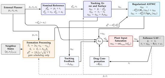
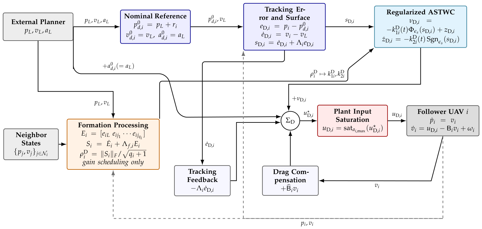
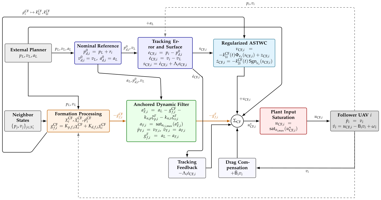
Figure 1 shows that formation information schedules the common gains but is not added to the D-ASTWC command.

Figure 1. D-ASTWC architecture for follower i. Formation information affects the adaptive gain scheduling signal, but no additive deformation cue is inserted into the nominal reference or final plant command. Gray blocks denote external signals and the plant, blue denotes reference and tracking computations, cyan denotes ASTWC, orange denotes formation processing, and red denotes saturation. Solid arrows indicate signal flow; dashed gray arrows indicate follower-state feedback.

4.3. C-ASTWC: Coordination-Input Adaptive Super-Twisting Control

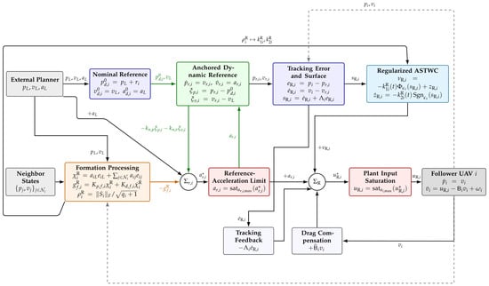
C-ASTWC retains the nominal reference and tracking surface but places the shared deformation cue directly in the plant input:

$$u_{\mathrm{C},i}^{\star }=a_L+{\widehat{\mathsf{B}}}_i{v}_i-{\Lambda }_i{\dot{e}}_{\mathrm{C},i}+{\nu }_{\mathrm{C},i}-g_{f,i}^{\mathrm{C}}.$$

(45)

Thus,

$${\dot{s}}_{\mathrm{C},i}={\nu }_{\mathrm{C},i}+{\vartheta }_i-g_{f,i}^{\mathrm{C}}+{\epsilon }_{a,i}^{\mathrm{C}}.$$

(46)

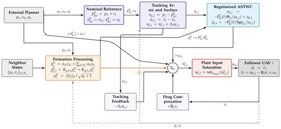
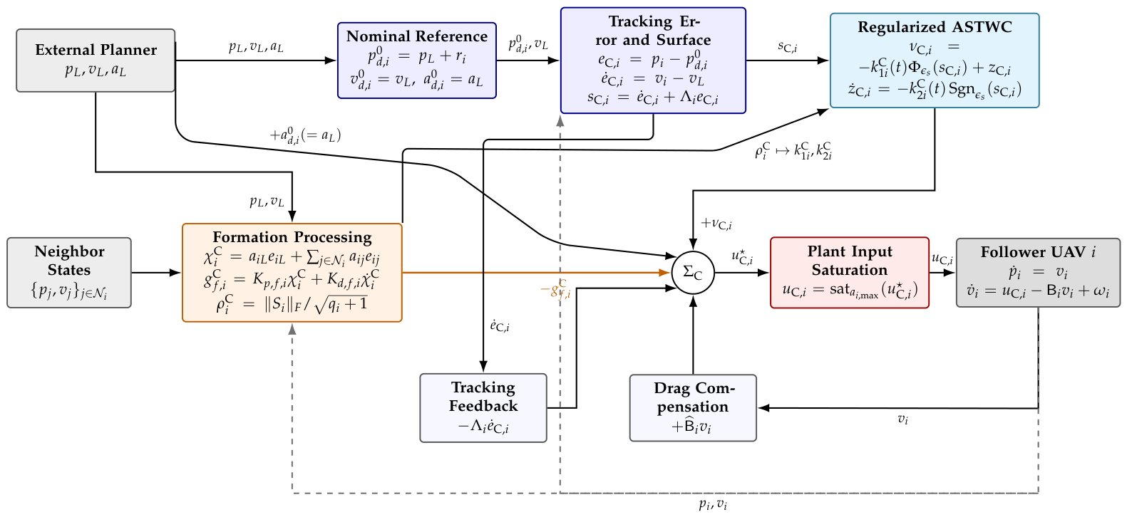
C-ASTWC is a controlled insertion-point comparator: it uses the same $K_{p,f,i}$ and $K_{d,f,i}$ as FR-ASTWC, but it does not redesign the tracking manifold or introduce a separate reference state. Its direct signal placement is summarized in Figure 2.

Figure 2. C-ASTWC architecture for follower i. The leader–neighbor deformation cue is placed directly in the final plant command, while the nominal leader offset reference is retained. Block colors and arrow styles follow Figure 1; orange arrows identify deformation-cue injection.

4.4. CF-ASTWC: Coordination-Filtered-Input Adaptive Super-Twisting Control

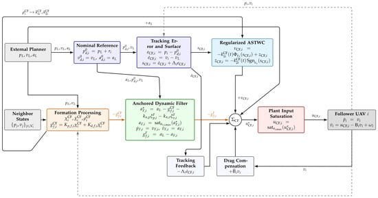
CF-ASTWC uses the same second-order filter and upstream limit as FR-ASTWC but retains the nominal tracking reference. The filter states $p_{F,i},v_{F,i}$ and the following deviations are introduced:

$${\xi }_{p,i}^F=p_{F,i}-p_{d,i}^0,{\xi }_{v,i}^F=v_{F,i}-v_L.$$

(47)

The positive anchoring gains $k_{n,p}$ and $k_{n,v}$ have units s⁻² and s⁻¹, respectively. The raw and implemented filter accelerations are

$$a_{F,i}^{\star }=a_L-g_{f,i}^{\mathrm{CF}}-k_{n,p}{\xi }_{p,i}^F-k_{n,v}{\xi }_{v,i}^F,$$

(48)

$$a_{F,i}={\mathrm{sat}}_{a_{r,i,\max }}\left(a_{F,i}^{\star }\right),{\dot{p}}_{F,i}=v_{F,i},{\dot{v}}_{F,i}=a_{F,i},$$

(49)

with $p_{F,i}\left(0\right)=p_{d,i}^0\left(0\right)$ and $v_{F,i}\left(0\right)=v_L\left(0\right)$. Define the filtered plant input cue

$$g_{f,i}^F=a_L-a_{F,i}.$$

(50)

CF-ASTWC tracks $p_{d,i}^0,v_L,a_L$, not $p_{F,i},v_{F,i},a_{F,i}$, and uses

$$u_{\mathrm{CF},i}^{\star }=a_L+{\widehat{\mathsf{B}}}_i{v}_i-{\Lambda }_i{\dot{e}}_{\mathrm{CF},i}+{\nu }_{\mathrm{CF},i}-g_{f,i}^F.$$

(51)

Therefore,

$${\dot{s}}_{\mathrm{CF},i}={\nu }_{\mathrm{CF},i}+{\vartheta }_i-g_{f,i}^F+{\epsilon }_{a,i}^{\mathrm{CF}}.$$

(52)

C versus CF isolates dynamic filtering; CF versus FR compares filtered input placement with tracking the dynamic reference. The shared filter law, parameters, and limit do not imply identical filter state or acceleration histories in independent closed-loop runs. Figure 3 displays this distinction.

Figure 3. CF-ASTWC architecture for follower i. The second-order filter law, parameters, and upstream limit match those of FR-ASTWC, but the nominal reference is retained and the filtered cue $g_{f,i}^F$ is injected at the final plant input sum. Block colors and arrow styles follow Figure 1 and Figure 2; the green block denotes the anchored dynamic filter.

4.5. FR-ASTWC: Formation-Reshaping Adaptive Super-Twisting Control

Define the reference deviations

$${\xi }_{p,i}=p_{r,i}-p_{d,i}^0,{\xi }_{v,i}=v_{r,i}-v_L={\dot{\xi }}_{p,i}.$$

(53)

The unsaturated reshaped acceleration is

$$\begin{array}{|c|}\hline a_{r,i}^{\star }=a_L-g_{f,i}^{\mathrm{R}}-k_{n,p}{\xi }_{p,i}-k_{n,v}{\xi }_{v,i},\\ \hline\end{array}$$

(54)

where $k_{n,p},k_{n,v}>0$. The implemented reference acceleration and its residual are

$$a_{r,i}={\mathrm{sat}}_{a_{r,i,\max }}\left(a_{r,i}^{\star }\right)=a_{r,i}^{\star }+{\epsilon }_{r,i}.$$

(55)

The reference states satisfy

$${\dot{p}}_{r,i}=v_{r,i},{\dot{v}}_{r,i}=a_{r,i},$$

(56)

with $p_{r,i}\left(0\right)=p_{d,i}^0\left(0\right)$ and $v_{r,i}\left(0\right)=v_L\left(0\right)$. Hence,

$${\ddot{\xi }}_{p,i}+k_{n,v}{\dot{\xi }}_{p,i}+k_{n,p}{\xi }_{p,i}=-g_{f,i}^{\mathrm{R}}+{\epsilon }_{r,i}.$$

(57)

The inner tracking error is

$$e_{\mathrm{R},i}=p_i-p_{r,i},{\dot{e}}_{\mathrm{R},i}=v_i-v_{r,i},$$

(58)

and the plant command is

$$u_{\mathrm{R},i}^{\star }=a_{r,i}+{\widehat{\mathsf{B}}}_i{v}_i-{\Lambda }_i{\dot{e}}_{\mathrm{R},i}+{\nu }_{\mathrm{R},i}.$$

(59)

Its sliding dynamics are

$${\dot{s}}_{\mathrm{R},i}={\nu }_{\mathrm{R},i}+{\vartheta }_i+{\epsilon }_{a,i}^{\mathrm{R}}.$$

(60)

The outer filter modifies the demanded trajectory without increasing the physical actuation capability. To expose the changed feedback, write $e_i^0=p_i-p_{d,i}^0$ and $s_i^0=(v_i-v_L)+{\Lambda }_i{e}_i^0$ along the respective closed-loop trajectory. Equations (53) and (34) give

$$s_{\mathrm{R},i}=s_i^0-{\xi }_{v,i}-{\Lambda }_i{\xi }_{p,i}.$$

(61)

Substituting (50) and (53) into the commands yields

$$\begin{array}{cc}\hfill u_{\mathrm{CF},i}^{\star }& =a_{F,i}+{\widehat{\mathsf{B}}}_i{v}_i-{\Lambda }_i(v_i-v_L)+{\nu }_{\mathrm{CF},i},\hfill \\ \hfill u_{\mathrm{R},i}^{\star }& =a_{r,i}+{\widehat{\mathsf{B}}}_i{v}_i-{\Lambda }_i(v_i-v_L)+{\Lambda }_i{\xi }_{v,i}+{\nu }_{\mathrm{R},i}.\hfill \end{array}$$

(62)

Thus, the changed tracking surface and reference velocity also change the inner correction; filtering an input cue alone does not reproduce FR feedback.

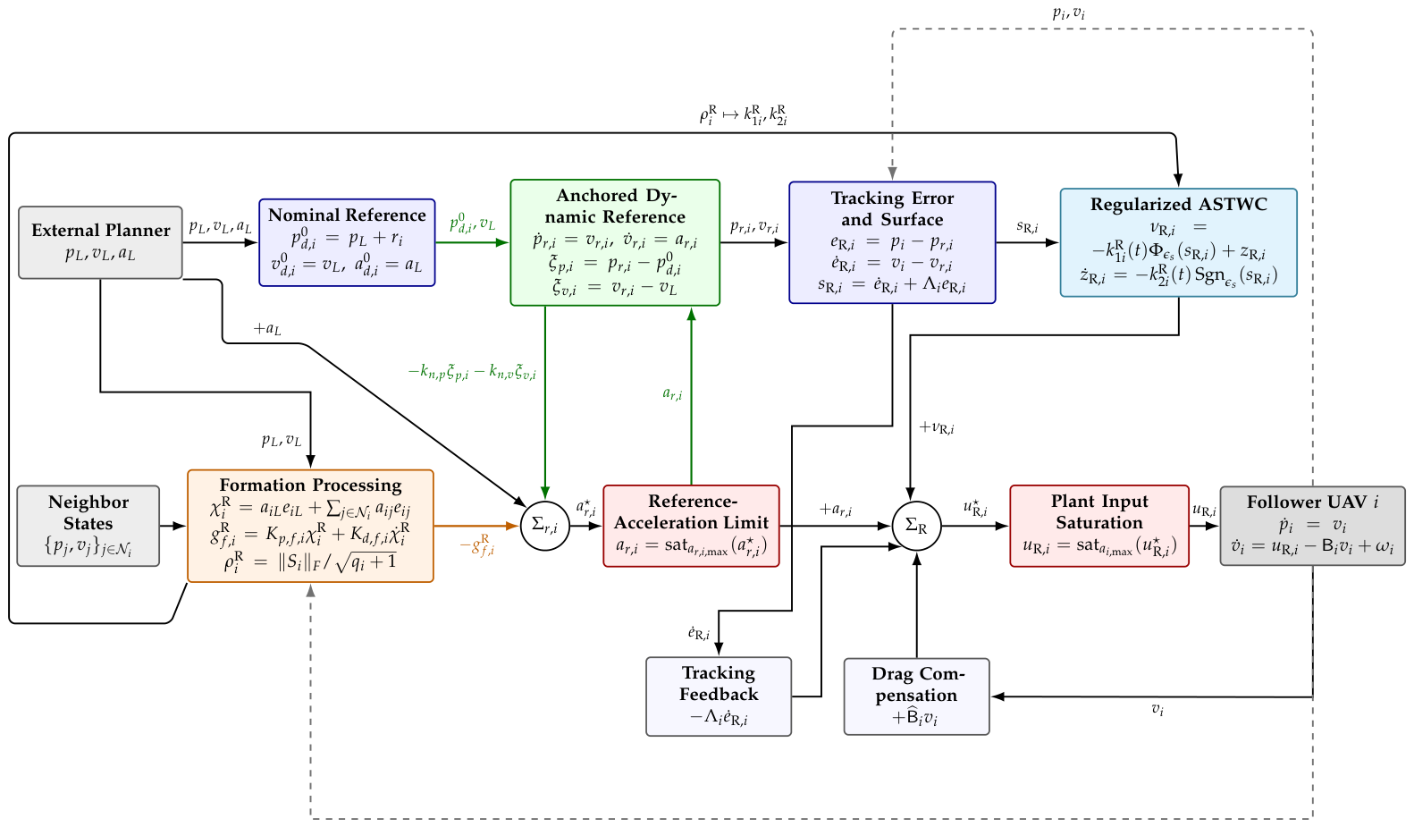
Figure 4 shows that the filtered states themselves, rather than only $g_{f,i}^F$, define the inner-loop target.

Figure 4. Proposed FR-ASTWC architecture for follower i. Formation deformation acts through an anchored, acceleration-limited dynamic reference before the common adaptive super-twisting tracking loop. Block colors and arrow styles follow Figure 1; orange arrows carry the deformation cue, while the green block and arrows identify dynamic reference generation and anchoring.

Proposition 1

(Residual and placement asymmetry). For the ideal unsaturated inner loops, the residual entering the super-twisting subsystem is

$${\delta }_i^{\mathrm{D}}={\delta }_i^{\mathrm{R}}={\vartheta }_i,{\delta }_i^{\mathrm{C}}={\vartheta }_i-g_{f,i}^{\mathrm{C}},{\delta }_i^{\mathrm{CF}}={\vartheta }_i-g_{f,i}^F.$$

(63)

Accordingly, a bound on ${\dot{\vartheta }}_i$ is sufficient for D-ASTWC and FR-ASTWC, whereas C-ASTWC and CF-ASTWC require an additional bound on the derivative of a closed-loop, state-dependent cue. Under ideal sliding, the equivalent corrections satisfy

$${\nu }_{\mathrm{D},i}^{\mathrm{eq}}={\nu }_{\mathrm{R},i}^{\mathrm{eq}}=-{\vartheta }_i,{\nu }_{\mathrm{C},i}^{\mathrm{eq}}=g_{f,i}^{\mathrm{C}}-{\vartheta }_i,{\nu }_{\mathrm{CF},i}^{\mathrm{eq}}=g_{f,i}^F-{\vartheta }_i.$$

(64)

On ideal sliding, each realization’s own tracking error satisfies ${\dot{e}}_{\mu ,i}=-{\Lambda }_i{e}_{\mu ,i}$. With ${\epsilon }_{r,i}=0$, FR-ASTWC additionally retains the stable target dynamics

$${\ddot{\xi }}_{p,i}+k_{n,v}{\dot{\xi }}_{p,i}+k_{n,p}{\xi }_{p,i}=-g_{f,i}^{\mathrm{R}}.$$

(65)

Thus, reference placement removes the deformation cue from the inner residual. With exact nominal drag, the remaining ${\vartheta }_i={\omega }_i$ is exogenous. This structural distinction does not assert uniformly lower deformation or saturation for every trajectory.

Proof. 

Equations (44), (46), (52) and (60) give (63). Setting each ideal sliding variable and its derivative to zero gives the equivalent corrections. The reduced error dynamics follow from the surface definitions, and the FR target dynamics follow from (57).    □

5. Stability and Practical Boundedness Analysis

The analysis separates the ideal discontinuous, unsaturated system from the regularized and occasionally saturated numerical realization. The ideal common certificate is restricted to D-ASTWC and FR-ASTWC by Proposition 1. C-ASTWC and CF-ASTWC remain empirical placement ablations, and the practical result is explicitly conditional on bounded implemented residuals. The hypotheses are the stated leader regularity with bounded velocity/acceleration and constant offsets, an absolutely continuous matched residual with a bounded magnitude and derivative, the fixed symmetric pinned graph, positive tracking/cue/anchor gains, and projected gains inside the certified box. Follower-dependent drag and acceleration limits are retained, but input feasibility is an additional premise of the ideal theorem. The tested deformation cue is continuous state feedback driven by smooth planned transitions; the analysis does not cover arbitrary reference state resets or switching graphs.

5.1. Graph Consequence

Lemma 1

(Local-to-global deformation bound). Under Assumption 4,

$$∥x∥\le {\lambda }_{\min }{\left(H\right)}^{-1}∥\chi ∥.$$

(66)

Consequently, bounded χ implies bounded leader-relative and neighbor-relative formation errors.

Proof. 

Equation (30) and the positive definiteness of H give (31). Since $e_{ij}=x_i-x_j$, every pairwise error is a linear function of x.    □

5.2. Common Ideal Super-Twisting Certificate

For one component of follower i, write the ideal residual-form dynamics as

$$\dot{s}=-k_1\left(t\right){\left|s\right|}^{1/2}\mathrm{sgn}\left(s\right)+y,\dot{y}=-k_2\left(t\right)\mathrm{sgn}\left(s\right)+\dot{\delta }\left(t\right),$$

(67)

where $|\dot{\delta }\left(t\right)|\le L_i$. For $s\ne 0$, define $\phi ={\left|s\right|}^{1/2}\mathrm{sgn}\left(s\right)$ and $\zeta ={\left[\phi y\right]}^{\mathsf{T}}$. Then,

$$\dot{\zeta }={\displaystyle \frac{1}{2\left|\phi \right|}}A(k_1,k_2,\eta )\zeta ,A(k_1,k_2,\eta )=\left[\begin{array}{cc}-k_1& 1\\ -2(k_2-\eta )& 0\end{array}\right],$$

(68)

where $\eta =\dot{\delta }\mathrm{sgn}\left(\phi \right)\in [-L_i,L_i]$.

Condition 1

(D/FR common gain certificate). For each follower i, there exist $P_i=P_i^{\mathsf{T}}\succ 0$ and ${\mu }_i>0$ such that

$$A_v^{\mathsf{T}}{P}_i+P_i{A}_v⪯-{\mu }_i{I}_2$$

(69)

for all eight vertices generated by

$$k_1\in \{{\underline{k}}_{1i},{\overline{k}}_{1i}\},k_2\in \{{\underline{k}}_{2i},{\overline{k}}_{2i}\},\eta \in \{-L_i^{\vartheta },L_i^{\vartheta }\},$$

(70)

where $L_i^{\vartheta }\ge {\mathrm{ess\; sup}}_t{∥{\dot{\vartheta }}_i\left(t\right)∥}_{\infty }$.

Because ${∥{\dot{\vartheta }}_i\left(t\right)∥}_{\infty }\le {∥{\dot{\vartheta }}_i\left(t\right)∥}_2$, Assumption 2 permits the conservative choice $L_i^{\vartheta }={\overline{\ell }}_i$. The numerical study instead uses the tighter componentwise bound in (73).

Because (69) is affine in $(k_1,k_2,\eta )$, the eight vertex inequalities certify the complete box; this is a standard polytopic common quadratic argument [36]. The matrix $P_i$ is follower-specific and common over the follower’s gain box and ideal D/FR residual model. It is constant, so gain rate terms do not enter its Lyapunov derivative. With $V={\zeta }^{\mathsf{T}}{P}_i\zeta$,

$$\dot{V}\le -c_i{V}^{1/2},c_i={\displaystyle \frac{{\mu }_i}{2\sqrt{{\lambda }_{\max }\left(P_i\right)}}},$$

(71)

which yields the conservative ideal reaching time estimate

$$T_i\le {\displaystyle \frac{4\sqrt{{\lambda }_{\max }\left(P_i\right)}}{{\mu }_i}}\sqrt{V\left(0\right)}.$$

(72)

For the nominal certificate audit, ${\widehat{\mathsf{B}}}_i={\mathsf{B}}_i$ and therefore ${\dot{\vartheta }}_i={\dot{\omega }}_i$. The disturbance derivative is evaluated analytically on the grid $t_k=k\Delta t$, $k=0,\dots ,$ 20,000, with $\Delta t=0.002$ s, for all three disturbance phase variants. The maximum below is taken over these sampled times, components, and phase variants and is enlarged by 15% plus $0.05$ m/s³:

$$L_i^{\vartheta }=1.15\underset{\ell ,t}{\max }\left|{\dot{\vartheta }}_{i\ell }\left(t\right)\right|+0.05.$$

(73)

Section 7.1 supplies the analytic intersample and post-horizon enclosure used in the numerical certificate audit; the sampled maximum alone is not the continuous-time bound. The certificate applies to the stated nominal disturbance family. In the Monte Carlo study, the true drag varies while the controller retains its nominal drag, so (7) contains a state-dependent mismatch term; the study is empirical and is not covered by the nominal numerical certificate. C-ASTWC and CF-ASTWC additionally require bounds on ${\dot{\vartheta }}_i-{\dot{g}}_{f,i}$; their realized slopes are a posteriori diagnostics.

5.3. Tracking Error Bound

For any realization,

$${\dot{e}}_{\mu ,i}=-{\Lambda }_i{e}_{\mu ,i}+s_{\mu ,i}.$$

(74)

Hence, if $s_{\mu ,i}$ is bounded,

$$∥e_{\mu ,i}\left(t\right)∥\le e^{-{\lambda }_{i}t}∥e_{\mu ,i}\left(0\right)∥+{\int }_0^t{e}^{-{\lambda }_i(t-\tau )}∥s_{\mu ,i}\left(\tau \right)∥d\tau ,$$

(75)

where ${\lambda }_i={\lambda }_{\min }\left({\Lambda }_i\right)$. In particular,

$$\underset{t\to \infty }{\mathrm{lim\; sup}}∥e_{\mu ,i}\left(t\right)∥\le {\lambda }_i^{-1}\underset{t\to \infty }{\mathrm{lim\; sup}}∥s_{\mu ,i}\left(t\right)∥.$$

(76)

Under ideal finite-time sliding, the tracking error converges exponentially to zero after reaching.

5.4. Anchored Reference Dynamics

Stack $\xi =\mathrm{col}({\xi }_{p,1},\dots ,{\xi }_{p,N})$ and $e_R=\mathrm{col}(e_{\mathrm{R},1},\dots ,e_{\mathrm{R},N})$. Since $x=e_R+\xi$ and $\chi =\overline{H}x$, the FR reference equation becomes

$$\ddot{\xi }+(k_{n,v}I+{\mathcal{K}}_{d,f}\overline{H})\dot{\xi }+(k_{n,p}I+{\mathcal{K}}_{p,f}\overline{H})\xi =-{\mathcal{K}}_{p,f}\overline{H}{e}_R-{\mathcal{K}}_{d,f}\overline{H}{\dot{e}}_R+{\epsilon }_r,$$

(77)

where ${\mathcal{K}}_{p,f}=\mathrm{blkdiag}(K_{p,f,1},\dots ,K_{p,f,N})$, ${\mathcal{K}}_{d,f}$ is defined similarly, and ${\epsilon }_r$ stacks the reference saturation residuals.

Let $y={\overline{H}}^{1/2}\xi$ and $e_y={\overline{H}}^{1/2}{e}_R$. Then,

$$\ddot{y}+C_y\dot{y}+K_{y}y=d_y,$$

(78)

where

$$C_y=k_{n,v}I+{\overline{H}}^{1/2}{\mathcal{K}}_{d,f}{\overline{H}}^{1/2}\succ 0,K_y=k_{n,p}I+{\overline{H}}^{1/2}{\mathcal{K}}_{p,f}{\overline{H}}^{1/2}\succ 0,$$

(79)

$$d_y=-{\overline{H}}^{1/2}{\mathcal{K}}_{p,f}{\overline{H}}^{1/2}{e}_y-{\overline{H}}^{1/2}{\mathcal{K}}_{d,f}{\overline{H}}^{1/2}{\dot{e}}_y+{\overline{H}}^{1/2}{\epsilon }_r.$$

(80)

The state $z_y=\mathrm{col}(y,\dot{y})$ has the system matrix

$$A_y=\left[\begin{array}{cc}0& I\\ -K_y& -C_y\end{array}\right],{\Gamma }_y=\left[\begin{array}{c}0\\ I\end{array}\right].$$

(81)

Because $C_y\succ 0$ and $K_y\succ 0$, the unforced system has energy $W_y=\frac{1}{2}{∥\dot{y}∥}^2+\frac{1}{2}{y}^{\mathsf{T}}{K}_{y}y$ and ${\dot{W}}_y=-{\dot{y}}^{\mathsf{T}}{C}_y\dot{y}\le 0$. LaSalle’s invariance principle implies asymptotic stability, so $A_y$ is Hurwitz. For any $Q_y=Q_y^{\mathsf{T}}\succ 0$, let $P_y=P_y^{\mathsf{T}}\succ 0$ solve

$$A_y^{\mathsf{T}}{P}_y+P_y{A}_y=-Q_y.$$

(82)

Then, $V_y=z_y^{\mathsf{T}}{P}_y{z}_y$ satisfies

$${\dot{V}}_y\le -{\alpha }_y{V}_y+{\beta }_y{∥d_y∥}^2,$$

(83)

with

$${\alpha }_y={\displaystyle \frac{{\lambda }_{\min }\left(Q_y\right)}{2{\lambda }_{\max }\left(P_y\right)}},{\beta }_y={\displaystyle \frac{2{∥P_y{\Gamma }_y∥}^2}{{\lambda }_{\min }\left(Q_y\right)}}.$$

(84)

Therefore the reshaped reference subsystem (78) is input-to-state stable (ISS) with respect to the input $d_y$ in the standard Lyapunov sense [37].

Theorem 1

(Ideal D/FR convergence). Suppose that Assumptions 1–4 and Condition 1 hold. For the ideal unregularized law with ${\epsilon }_{a,i}^{\mathrm{D}}={\epsilon }_{a,i}^{\mathrm{R}}=0$ throughout, the inner D-ASTWC and FR-ASTWC sliding variables reach zero in finite time. Their tracking errors subsequently converge exponentially. For FR-ASTWC, if ${\epsilon }_r=0$, then $e_R\to 0$, $\xi \to 0$, and $x=e_R+\xi \to 0$.

Proof. 

For D-ASTWC and FR-ASTWC, Proposition 1 gives ${\delta }_i={\vartheta }_i$, so Condition 1 and (71) establish finite-time reaching componentwise. Equation (74) gives exponential tracking after reaching. For FR-ASTWC, (78) is asymptotically stable with vanishing $e_R$, ${\dot{e}}_R$, and ${\epsilon }_r$; hence, $\xi \to 0$ and $x=e_R+\xi \to 0$.    □

For the implementation bound, define $s_R=\mathrm{col}(s_{\mathrm{R},1},\dots ,s_{\mathrm{R},N})$ and $\mathsf{\Lambda }=\mathrm{blkdiag}({\Lambda }_1,\dots ,{\Lambda }_N)$.

Proposition 2

(Conditional practical FR bound). For the regularized and saturated implementation, suppose that

$$\underset{t\to \infty }{\mathrm{lim\; sup}}∥s_R\left(t\right)∥\le \overline{s},\underset{t\to \infty }{\mathrm{lim\; sup}}∥{\epsilon }_r\left(t\right)∥\le {\overline{\epsilon }}_r.$$

(85)

Then, the tracking error, reshaped reference deviation, and global formation error are ultimately bounded under the stated assumptions. One admissible conditional bound has the form

$$\mathrm{lim\; sup}∥x∥\le \overline{e}+{\displaystyle \frac{1}{\sqrt{{\lambda }_{\min }\left(H\right)}}}\sqrt{{\displaystyle \frac{{\beta }_y}{{\alpha }_y{\lambda }_{\min }\left(P_y\right)}}}{\overline{d}}_y,$$

(86)

where $\overline{e}\le {\lambda }_{\min }{(\mathsf{\Lambda })}^{-1}\overline{s}$ and ${\overline{d}}_y$ follows from (80) using the bounds on $e_R$, ${\dot{e}}_R$, and ${\epsilon }_r$.

Proof. 

Equation (76) bounds $e_R$, and ${\dot{e}}_R=-\mathsf{\Lambda }{e}_R+s_R$ is therefore bounded. Equation (83) bounds $z_y$, while $∥\xi ∥\le {\lambda }_{\min }{\left(H\right)}^{-1/2}∥y∥$. Finally, $x=e_R+\xi$ gives (86).    □

The finite-horizon simulation observations are consistent with the boundedness premises in Proposition 2; they do not establish these asymptotic premises. These premises are not consequences of Assumptions 1–4. The proposition is therefore an implication and not a global stability theorem for the saturated nonlinear implementation.

Remark 1

(Scope of C-ASTWC and CF-ASTWC). No ideal finite-time certificate is claimed for C-ASTWC or CF-ASTWC with the selected gain box. Their state-dependent residuals in (63) require additional cue derivative bounds. The complete realized envelope fails the necessary ${\underline{k}}_2-L>0$ margin for followers 1 and 2—most severely for the lower-capability follower 2. These controllers are retained as numerical placement ablations; increasing $k_2$ and retuning every controller is outside the scope of the controlled comparison.

Remark 2

(Actuation and safety scope). The reference limit $a_{r,i,\max }<a_{i,\max }$ is an upstream demand allocation setting. Indeed, (59) gives

$$∥u_{\mathrm{R},i}^{\star }∥\le a_{r,i,\max }+∥{\widehat{\mathsf{B}}}_i{v}_i-{\Lambda }_i{\dot{e}}_{\mathrm{R},i}+{\nu }_{\mathrm{R},i}∥.$$

(87)

Without a bound on the second term, the reference cap does not guarantee final-command feasibility or reduced saturation exposure. The reference integrator has no separate anti-windup state; anchoring supplies restoring feedback, but global windup exclusion is not proven. Likewise, the preplanned obstacle trajectory yields a numerical clearance margin, not a collision avoidance theorem. Formal input admissibility or collision avoidance would require an invariant set, barrier function, constrained optimization, or comparable safety layer.

6. Simulation Configuration and Evaluation Protocol

6.1. Heterogeneous Followers and Graph

The numerical study uses one leader and three followers. The complete undirected follower graph has neighbor weight $a_{ij}=0.275$ and leader-pinning weight $a_{iL}=0.45$, giving

$$H=\left[\begin{array}{ccc}1& -0.275& -0.275\\ -0.275& 1& -0.275\\ -0.275& -0.275& 1\end{array}\right],$$

(88)

with eigenvalues $\{0.45,1.275,1.275\}$. Hence, Lemma 1 gives $∥x∥\le (1/0.45)∥\chi ∥\approx 2.22∥\chi ∥$. The desired follower offsets are the columns of

$$\Delta =\left[\begin{array}{ccc}-2.0& -2.0& -4.0\\ -1.5& 1.5& 0.0\\ 0.0& 0.0& 0.0\end{array}\right]\mathrm{m}.$$

(89)

The initial leader state is $p_L\left(0\right)={[0,0,2]}^{\mathsf{T}}$ m and $v_L\left(0\right)={[0.58,0,0]}^{\mathsf{T}}$ m/s. In the nominal and deterministic scenario studies, each follower starts at $p_i\left(0\right)=p_L\left(0\right)+r_i$ and $v_i\left(0\right)=v_L\left(0\right)$, so the reported errors are not dominated by initial condition recovery. Table 3 lists the heterogeneous physical descriptors and mass-normalized plant parameters; $R_i$ denotes the spherical reporting radius of follower i.

Table 3. Heterogeneous follower parameters. $D_i=m_i{\beta }_i$ is reported for the isotropic physical drag model.

Follower	${\mathit{m}}_{\mathit{i}}$ [kg]	${\mathit{\beta }}_{\mathit{i}}$ [s−1]	${\mathit{D}}_{\mathit{i}}$ [kg/s]	${\mathit{a}}_{\mathit{i},\max }^0$ [m/s2]	${\mathit{R}}_{\mathit{i}}$ [m]	${\mathit{r}}_{\mathit{i}}$ [m]
1	1.10	0.16	0.1760	3.00	0.35	${[-2.0,-1.5,0]}^{\mathsf{T}}$
2	1.35	0.23	0.3105	2.70	0.45	${[-2.0,1.5,0]}^{\mathsf{T}}$
3	0.95	0.19	0.1805	3.30	0.30	${[-4.0,0,0]}^{\mathsf{T}}$

The superscript $\mathsf{T}$ denotes transposition.

Every controller uses the common settings in Table 4.

Table 4. Controller and numerical parameters.

Quantity	Value
Sampling interval and horizon	$\Delta t=0.002$ s, $T=40$ s
Formation sliding gain	${\Lambda }_{f,i}=0.90I_3$
Cue gains $(K_{p,f,i},K_{d,f,i})$	$(1.40,0.80)$, $(1.35,0.76)$, $(1.45,0.84)$
Tracking gains ${\Lambda }_i$	$1.45I_3$, $1.35I_3$, $1.55I_3$
Anchoring gains	$k_{n,p}=2.40$ s−2, $k_{n,v}=3.45$ s−1
STA gain boxes (common to all followers)	$k_{1i}\in [4,6]$, $k_{2i}\in [4,5]$ (consistent SI-derived units)
Initial controller/filter states	$k_{1i}\left(0\right)=k_{2i}\left(0\right)=4$, $z_i\left(0\right)=0$; $p_{F,i}\left(0\right)=p_{r,i}\left(0\right)=p_{d,i}^0\left(0\right)$ and $v_{F,i}\left(0\right)=v_{r,i}\left(0\right)=v_L\left(0\right)$
Gain scheduler	${\gamma }_{1i}=1.0$, ${\gamma }_{2i}=0.8$, ${\sigma }_{1i}=0.45$, ${\sigma }_{2i}=0.50$
Regularization	${ϵ}_s={10}^{-3}$
CF/FR upstream acceleration limit	$a_{r,i,\max }=0.90a_{i,\max }$
Integration	Explicit first-order velocity/controller state update; constant-acceleration position update

The scalar cue coefficients in Table 4 multiply $I_3$ and have units s⁻² and s⁻¹. The deformation cue combines the proportional restoration of the weighted shape error with damping through its measured rate; it uses no obstacle distance input. The positive anchor gains restore the dynamic reference toward the nominal leader offset. In isolation, the anchor polynomial $s^2+3.45s+2.40$ has poles $-0.9663$ and $-2.4837$ s⁻¹, natural frequency $1.5492$ rad/s, and damping ratio $1.1135$. These values describe an overdamped nominal return, not optimal tuning or the complete saturated response. The nominal limit ratio $0.90$ reserves part of the acceleration budget for tracking and drag compensation but does not guarantee final-command feasibility. The sensitivity experiment described below varies these design choices while fixing the inner tracker.

The simulations were performed using MATLAB R2024b on 64-bit Windows. At each step, the formation signals, reference acceleration, sliding correction, and saturated plant command are evaluated from the current states. The plant acceleration gives $v_{k+1}=v_k+\Delta t{\dot{v}}_k$ and $p_{k+1}=p_k+\Delta t{v}_k+\frac{1}{2}\Delta t^2{\dot{v}}_k$; the controller and reference velocity states use explicit updates, and the reference position uses the corresponding constant-acceleration update. The archived scripts contain the exact update order, normalized directions, configurations, and figure/metric routines. The validation runner and direct certificate check require no optimization, statistics, or parallel computing toolbox. This is a fixed-step simulation, not a measured real-time implementation.

6.2. Directionally Heterogeneous Disturbances

Every controller is subjected to the same smooth, directionally heterogeneous matched disturbances. Let $e_{1i}$ and $e_{2i}$ be the ith columns of the normalized direction matrices $D_p$ and $D_s$. The injected acceleration disturbance is

$${\omega }_i\left(t\right)=b_i\left(t\right)+d_{I,i}\left(t\right)+g_i\left(t\right),$$

(90)

where

$$\begin{array}{cc}\hfill b_i\left(t\right)& =A_{b,i}\left[0.70\sin (0.38t+0.40i)e_{1i}+0.45\cos (0.31t+0.75i)e_{2i}\right],\hfill \end{array}$$

(91)

$$\begin{array}{cc}\hfill d_{I,i}\left(t\right)& =A_{I,i}{\upsilon }_i\left(t\right)\left[\sin ({\omega }_{1i}{\tau }_i+{\varphi }_{1i})e_{1i}+0.65\cos ({\omega }_{2i}{\tau }_i+{\varphi }_{2i})e_{2i}\right],\hfill \end{array}$$

(92)

$$\begin{array}{cc}\hfill g_i\left(t\right)& =A_{G,i}\exp \left[-{\left({\displaystyle \frac{t-t_{G,i}}{{\sigma }_{G,i}}}\right)}^2\right](0.85e_{1i}-0.35e_{2i}).\hfill \end{array}$$

(93)

Here, ${\tau }_i=t-t_{I,i}^{\mathrm{on}}$ and ${\upsilon }_i\left(t\right)=\frac{1}{2}[1-\cos (2\pi {\tau }_i/T_i)]$ inside the interval $[t_{I,i}^{\mathrm{on}},t_{I,i}^{\mathrm{off}}]$, with $T_i=t_{I,i}^{\mathrm{off}}-t_{I,i}^{\mathrm{on}}$; $d_{I,i}=0$ outside this interval. The follower-specific intervals are

$$T_{d,1}=[12.30,16.35]\mathrm{s},T_{d,2}=[13.20,17.25]\mathrm{s},T_{d,3}=[14.00,18.05]\mathrm{s},$$

(94)

so the complete union is $T_d=[12.30,18.05]$ s. The effective interval amplitudes are $1.5066$, $1.29735$, and $1.71585$ m/s². The displayed normalized primary and secondary directions are rounded to four decimals and are the columns of

$$D_p=\left[\begin{array}{ccc}0.9305& -0.2921& -0.7111\\ -0.3257& 0.9249& -0.5588\\ 0.1675& 0.2434& -0.4267\end{array}\right],D_s=\left[\begin{array}{ccc}-0.2005& 0.4490& 0.3017\\ 0.3008& 0.0998& 0.7542\\ 0.9324& -0.8880& 0.5832\end{array}\right].$$

(95)

For exact reproduction, normalize each column of the following unrounded primary and secondary seeds, respectively:

$$\left[\begin{array}{ccc}1& -0.30& -0.70\\ -0.35& 0.95& -0.55\\ 0.18& 0.25& -0.42\end{array}\right],\left[\begin{array}{ccc}-0.20& 0.45& 0.30\\ 0.30& 0.10& 0.75\\ 0.93& -0.89& 0.58\end{array}\right].$$

(96)

The base amplitudes are $[0.0871875,0.0775000,0.0968750]$ m/s². The frequency vectors are $[2.30,1.85,2.65]$ and $[1.55,2.20,1.35]$ rad/s, with phase vectors $[0.30,1.15,2.05]$ and $[1.20,0.45,1.70]$ rad. The Gaussian gust centers, amplitudes, and widths are $[23.70,25.00,26.05]$ s, $[0.8649,1.00905,0.792825]$ m/s², and $[0.75,0.95,0.85]$ s. Equation (90) is differentiated analytically for the certificate audit. No observer-derived cue is inserted into the reference.

6.3. Obstacle-Induced Leader Maneuver

The leader has a constant longitudinal speed ${\dot{x}}_L=0.58$ m/s and altitude $z_L=2$ m; its total speed varies during lateral transitions. Let $h\left(\tau \right)=10{\tau }^3-15{\tau }^4+6{\tau }^5$. The lateral path is $y_L\left(t\right)=3.5h((t-17)/3)$ on $[17,20]$ s, is held at $3.5$ m on $[20,32]$ s, and returns as $y_L\left(t\right)=3.5[1-h((t-32)/3)]$ on $[32,35]$ s; otherwise, $y_L=0$. The position, velocity, and acceleration are continuous, and the lateral velocity and acceleration vanish at each junction; jerk is piecewise continuous and changes at the splice times. The peak lateral speed and acceleration are $2.1875$ m/s and $2.2453$ m/s², respectively. The spherical obstacle has center $p_o={[13.5,0,2]}^{\mathsf{T}}$ m and radius $R_o=1$ m. Plant velocity and controller states use a fixed explicit first-order step $\Delta t=0.002$ s, whereas the position uses the constant-acceleration kinematic update over each step. The active acceleration-producing intervals are

$$T_{o,a}=[17,20]\cup [32,35]\mathrm{s}.$$

(97)

The common path is generated outside the compared controllers. Accordingly, the experiment evaluates formation maintenance during an obstacle-induced maneuver, rather than proposing an obstacle avoidance algorithm.

Table 5 compares the peak planned lateral acceleration with the follower limits. The 85% case is the marginal plant-kinematic regime: every final plant limit exceeds $2.2453$ m/s², but follower 2 has only $0.0497$ m/s² nominal headroom and its CF/FR upstream setting is lower than the peak. This feedforward comparison is necessary but not sufficient for complete feasibility because drag compensation, disturbances, and feedback share the same final channel.

Table 5. Peak planned lateral acceleration versus follower-specific final limits and CF/FR upstream limits. Parentheses give final-limit headroom relative to $2.2453$ m/s².

Capability	${\mathit{a}}_{1,\max }$	${\mathit{a}}_{2,\max }$	${\mathit{a}}_{3,\max }$	${\mathit{a}}_{\mathit{r},1,\max }$	${\mathit{a}}_{\mathit{r},2,\max }$	${\mathit{a}}_{\mathit{r},3,\max }$
	Final Limit [m/s2] (Headroom)			Upstream Limit [m/s2]
100%	3.0000 (0.7547)	2.7000 (0.4547)	3.3000 (1.0547)	2.7000	2.4300	2.9700
85%	2.5500 (0.3047)	2.2950 (0.0497)	2.8050 (0.5597)	2.2950	2.0655	2.5245
70%	2.1000 ($-0.1453$)	1.8900 ($-0.3553$)	2.3100 (0.0647)	1.8900	1.7010	2.0790

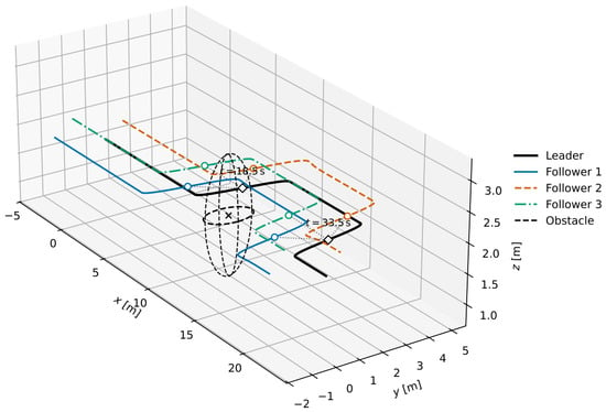
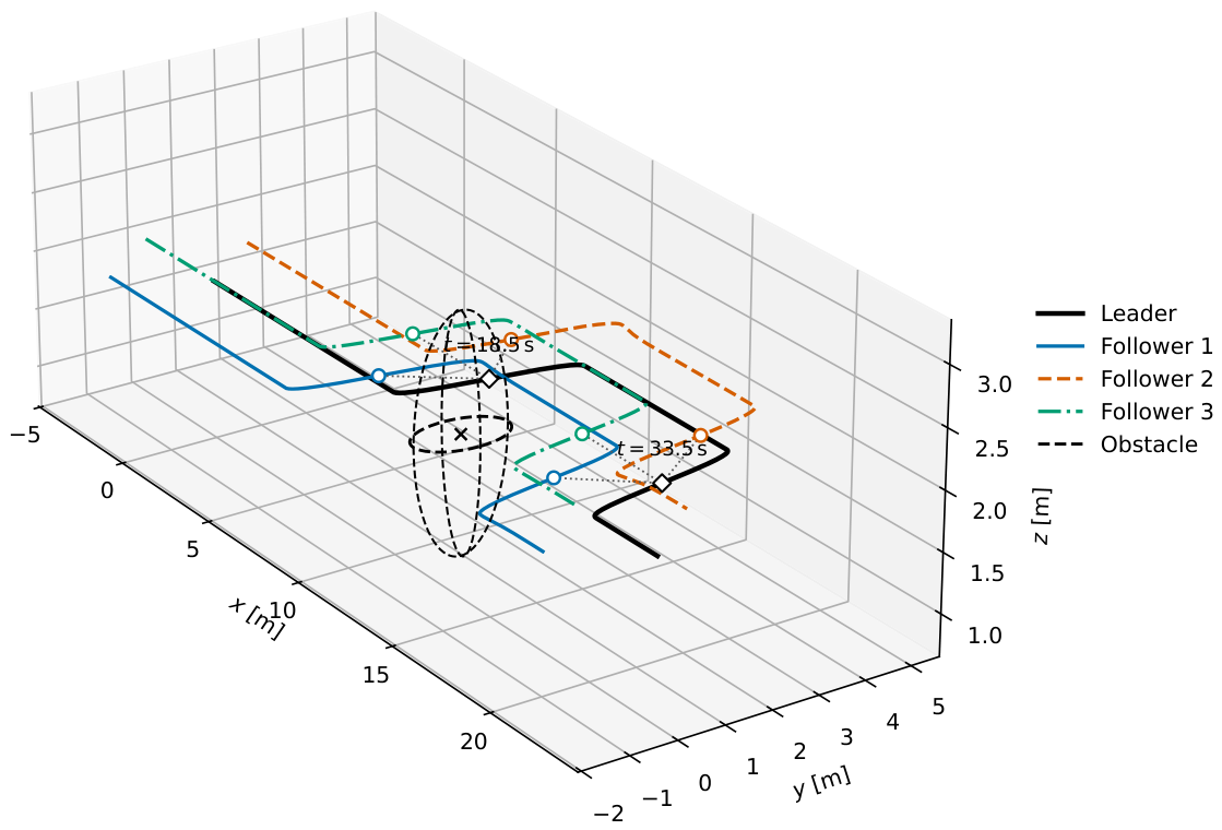
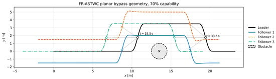
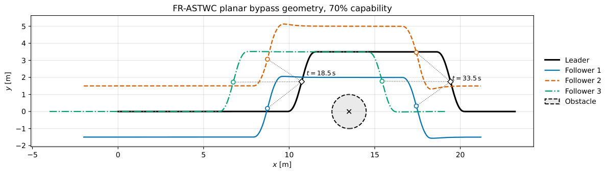
Figure 5 and Figure 6 show elevated and planar views of the FR-ASTWC bypass geometry in the 70% reference run. They illustrate the common scenario rather than comparing controllers; the numerical clearance values are reported separately in Section 7.5.

Figure 5. Single-panel three-dimensional view of the FR-ASTWC obstacle bypass geometry at 70% available translational actuation capability. Synchronous snapshots distinguish simultaneous UAV configurations from complete trajectory curves. The panel is illustrative and is not used for controller discrimination; the positive clearance is a numerical scenario result rather than a formal collision avoidance guarantee.

Figure 6. Planar view of the same FR-ASTWC reference run as in Figure 5. This panel shows the bypass geometry and obstacle separation without making a visual controller comparison claim; exact required clearance values are given in Section 7.5.

6.4. Available Actuation Capability Sweep and Metrics

The nominal limits $a_{i,\max }^0$ are scaled as

$$a_{i,\max }^{\left(\alpha \right)}=\alpha a_{i,\max }^0,\alpha \in \{1.00,0.85,0.70\}.$$

(98)

The word capability refers only to the maximum translational acceleration command available before saturation. It does not imply communication or decision authority. The common CF/FR upstream limit is $0.90a_{i,\max }^{\left(\alpha \right)}$.

Define the mean deformation and intensity

$$\overline{\chi }\left(t\right)={\displaystyle \frac{1}{N}}{\displaystyle \sum _{i=1}^N}∥{\chi }_i\left(t\right)∥,\overline{\rho }\left(t\right)={\displaystyle \frac{1}{N}}{\displaystyle \sum _{i=1}^N}{\rho }_i\left(t\right).$$

(99)

For full-horizon reporting, the leader error is $e_{iL}$, the neighbor error is $e_{ij}$ over unique undirected edges, and the deformation error is ${\chi }_i$. For a sampled vector error $r_m\left(t_k\right)$ over a time index set $\mathcal{I}$ and M followers or graph edges, the reported root mean square error (RMSE) is

$$\mathrm{RMSE}\left(r\right)=\sqrt{{\displaystyle \frac{1}{\left|\mathcal{I}\right|M}}\sum _{k\in \mathcal{I}}\sum _{m=1}^M{∥r_m\left(t_k\right)∥}^2}.$$

(100)

Let ${\mathcal{I}}_a=\{k:t_k\in T_{o,a}\}$. The active peak and active-window mean are

$${\chi }_{\mathrm{pk},a}=\underset{k\in {\mathcal{I}}_a}{\max }\overline{\chi }\left(t_k\right),{\chi }_{\mathrm{mean},a}={\displaystyle \frac{1}{|{\mathcal{I}}_a|}}\sum _{k\in {\mathcal{I}}_a}\overline{\chi }\left(t_k\right).$$

(101)

The plant saturation duty over an index set $\mathcal{I}$ is

$$D_{u,\mathcal{I}}={\displaystyle \frac{100}{N\left|\mathcal{I}\right|}}\sum _{k\in \mathcal{I}}{\displaystyle \sum _{i=1}^N}\mathbf{1}\{∥u_i^{\star }\left(t_k\right)∥>a_{i,\max }+{10}^{-12}\},$$

(102)

where ${10}^{-12}$ m/s² is the numerical comparison tolerance. The denominator counts follower–time samples, rather than only times when at least one follower saturates. Upstream duty uses $∥a_{F,i}^{\star }∥>a_{r,i,\max }$ for CF-ASTWC and $∥a_{r,i}^{\star }∥>a_{r,i,\max }$ for FR-ASTWC, with the same ${10}^{-12}$ m/s² comparison tolerance. The applied and commanded control demand integrals are

$$J_u={\int }_{\mathcal{T}}\sum _i{∥u_i\left(t\right)∥}^{2}dt,J_{u^{\star }}={\int }_{\mathcal{T}}\sum _i{∥u_i^{\star }\left(t\right)∥}^{2}dt,$$

(103)

with units m²/s³; they are not electrical energy. Other reported quantities are the peak and mean of $\overline{\chi }$ and $\overline{\rho }$ over $T_{o,a}$, peak $∥u_i^{\star }∥$, and maximum $∥p_{r,i}-p_{d,i}^0∥$. Window sensitivity is assessed through the extended-window sample mean

$${\overline{\chi }}_{\mathrm{ext}}={\displaystyle \frac{1}{|{\mathcal{I}}_e|}}\sum _{k\in {\mathcal{I}}_e}\overline{\chi }\left(t_k\right),{\mathcal{I}}_e=\left\{k:t_k\in [17,23]\cup [32,38]\mathrm{s}\right\}.$$

(104)

Both active and extended masks include their endpoints. With $\Delta t=0.002$ s, they contain 3002 and 6002 samples, respectively; the complete horizon contains 20001 samples. The tables and captions distinguish these windows explicitly. Active-window effort is evaluated by trapezoidal integration separately over $[17,20]$ and $[32,35]$ s, with their endpoints included. This removes the small half-step contributions outside these intervals that arose from applying the full-grid trapezoidal rule to zero-masked power in the original reporting code. All active effort entries here use the corrected convention. The archived legacy columns permit comparison; deformation, saturation, recovery, and full-horizon effort values are unaffected.

For a nonnegative metric M, the within-scenario relative reduction is $R_j=100(M_{B,j}-M_{\mathrm{FR},j})/M_{B,j}$, where B denotes the paired comparator. The reported mean paired percentage is $n^{-1}{\sum }_j{R}_j$, not the percentage formed from two aggregate means. Absolute differences are $M_{B,j}-M_{\mathrm{FR},j}$; positive values favor FR. Percentage reductions are undefined when $M_{B,j}\le {10}^{-12}$, including zero-saturation cases, and are not assigned a value of zero.

For numerical clearance reporting, $d_{\mathrm{req}}=0.20$ m is the obstacle buffer and $d_{\mathrm{sep}}=0.20$ m is the inter-UAV buffer; $p_o$, $R_o$, and $R_i$ denote the obstacle center, obstacle radius, and follower radii.

6.5. Filtered Input and Scenario Variation Protocol

The capability sweep evaluates D-ASTWC, C-ASTWC, CF-ASTWC, and FR-ASTWC under the same positive-y bypass and disturbance realization. C versus CF tests whether dynamic cue filtering alone helps, while CF versus FR compares input placement and reference placement using the same second-order filter, upstream limit, cue gains, and initial filter states.

To test sensitivity to scenario details, the 70% capability experiment is repeated for bypass signs $b_y\in \{+1,-1\}$ and three deterministic disturbance phase pairs,

$$(\Delta {\varphi }_1,\Delta {\varphi }_2)\in \{(0,0),(0.37,-0.29),(-0.41,0.33)\}\mathrm{rad}.$$

(105)

The sign $b_y$ multiplies the lateral bypass amplitude, while the phase offsets are applied uniformly across followers to the two interval disturbance sinusoidal components. The resulting ensemble contains $2\times 3\times 4=24$ simulations. The results are reported as the mean and range across the six scenario variants for each controller.

6.6. Design Parameter Sensitivity

A one-at-a-time experiment scales each group of proportional cue gains, derivative cue gains, proportional anchor gains, or derivative anchor gains by $0.75$ and $1.25$ relative to Table 4. The upstream/final limit ratio is separately set to $0.80$, $0.85$, and $0.95$, around the nominal $0.90$. The nominal case is counted once, yielding 12 settings at three capability levels for four controllers (144 simulations). Other settings, including the gain boxes, adaptation, regularization, step size, positive bypass direction, and disturbances, remain nominal. This is a local tuning sensitivity test, not controller-specific optimization. D has no additive cue; anchor and upstream limit changes affect only CF and FR.

6.7. Paired Monte Carlo Protocol

The randomized study uses 100 independent scenario draws, each evaluated by all four controllers at each of the three capability levels (1200 simulations). Draws are generated and saved before simulation using a local MATLAB mt19937ar stream with seed 4592842. The same draw is reused across controllers and capability levels; the statistical unit is the scenario, not the 1200 individual runs. Table 6 specifies the joint perturbations. Unless linked by this pairing, sampled components and parameters are independent. The ranges were selected as stress test intervals, not calibrated distributions of a physical UAV population. Inner-loop gains are not retuned.

Table 6. Prespecified joint-uncertainty design for the paired Monte Carlo study. Unlisted parameters retain their nominal values.

Quantity	Distribution or Setting
Bypass direction	$+y$ or $-y$, each with probability $1/2$
True normalized drag	Independent $U[0.90,1.10]{\beta }_i$ for each follower; ${\widehat{\beta }}_i$ remains nominal
Plant acceleration limit	Independent $U[0.95,1.05]\alpha a_{i,\max }^0$ for each follower
Disturbance amplitudes	Independent $U[0.80,1.20]$ multipliers for each follower’s background, interval, and gust amplitudes
Interval disturbance phases	Each nominal phase plus an independent $U[-\pi ,\pi ]$ rad offset
Initial follower position	Each component of $p_i\left(0\right)-p_L\left(0\right)-r_i$ independently $U[-0.10,0.10]$ m; initial velocities and filter/reference states remain nominal

The three primary endpoints are the active peak deformation, active-window mean deformation, and active plant saturation duty. Extended-window means, full-horizon RMSEs, effort, clearance, and recovery are secondary checks. For each capability and comparator, 95% percentile intervals for the mean paired improvement use 2000 scenario bootstrap resamples with a separate mt19937ar stream (seed 4592843). Each resample preserves the controller pairing. Absolute and finite-percentage differences are summarized separately. The intervals are pointwise, with no multiple-comparison correction, and describe uncertainty under this specified sampling design. The six deterministic cases receive descriptive ranges only. Failed runs, incomplete pairs, negative clearances, and the absence of a complete 0.5 s recovery hold before 40 s are retained in the reporting files. Finite-horizon empirical outcomes do not extend the nominal ideal certificate to drag mismatch or new disturbance amplitudes/phases.

An AI assistant was used to refine the implementation code and cross-check numerical consistency. The author specified, executed, and verified the simulation model, controller formulations, parameters, and all reported results.

7. Results

7.1. D/FR Super-Twisting Certificate and C/CF Residual Audit

The direct MATLAB certificate audit passed all 24 gain box vertices (eight per follower), without gain retuning. The analytic derivative of (90) was sampled over $[0,40]$ s at $\Delta t=0.002$ s for all three phase variants. The raw sampled componentwise maxima are $3.03469546$, $2.22736799$, and $3.22399827$ m/s³. Applying (73) gives the D/FR envelopes in Table 7. For each trace-normalized $P_i$, the direct evaluation of all eight vertices gives ${\mu }_i>0$ and ${\underline{k}}_2-L_i^{\vartheta }>0$. The last column reports the conservative coefficient multiplying $\sqrt{V\left(0\right)}$ in (72); it is not an observed settling time.

Table 7. Directly verified common quadratic certificates for the ideal D-ASTWC and FR-ASTWC residual ${\delta }_i={\vartheta }_i$. Matrices are reported to ten decimal places and satisfy $\mathrm{tr}\left(P_i\right)=1$.

Follower	${\mathit{L}}_{\mathit{i}}^{\mathit{\vartheta }}$ [m/s3]	${\mathit{P}}_{\mathit{i}}$	${\mathit{\lambda }}_{\min }\left({\mathit{P}}_{\mathit{i}}\right)$	${\mathit{\mu }}_{\mathit{i}}$	$4-{\mathit{L}}_{\mathit{i}}^{\mathit{\vartheta }}$	Reaching Coefficient
1	3.5398997700	$\left[\begin{array}{cc}0.8736419274& -0.1680085109\\ -0.1680085109& 0.1263580726\end{array}\right]$	0.0903231155	0.0288220248	0.4601002300	132.3668
2	2.6114731900	$\left[\begin{array}{cc}0.8585861796& -0.1678697969\\ -0.1678697969& 0.1414138204\end{array}\right]$	0.1040652618	0.1016271458	1.3885268100	37.2553
3	3.7575980100	$\left[\begin{array}{cc}0.8786020719& -0.1748041991\\ -0.1748041991& 0.1213979281\end{array}\right]$	0.0829915625	0.0126209040	0.2424019900	303.4983

The continuous-time bound follows from the analytic disturbance profile. Using unit disturbance directions, $|{\upsilon }_i|\le 1$, $|{\dot{\upsilon }}_i|\le \pi /T_i$, $|{\ddot{\upsilon }}_i|\le 2{\pi }^2/T_i^2$, and the Gaussian envelope second-derivative bound $2/{\sigma }_{G,i}^2$ gives ${∥{\ddot{\omega }}_i\left(t\right)∥}_{\infty }\le 30$ m/s⁴ almost everywhere for every follower and phase variant. Since ${\dot{\omega }}_i$ is continuous, any componentwise derivative peak between adjacent samples exceeds the sampled maximum by at most $30\Delta t/2=0.030$ m/s³, which is below the additive $0.05$ m/s³ allowance in (73). For $t>40$ s, the interval disturbance vanishes, and the background-plus-Gaussian derivative is bounded by $1.23$ m/s³, below every reported $L_i^{\vartheta }$. Thus, the reported envelopes also bound the continuous-time disturbance derivatives for $t\ge 0$.

As an a posteriori diagnostic, including the realized C-ASTWC and CF-ASTWC residuals over all six scenarios gives enlarged envelopes $[4.3929864,8.6619017,3.8644136]$ m/s³. The corresponding necessary margins $4-L$ are $[-0.3929864,-4.6619017,0.1355864]$ m/s³. Thus, a common all-controller certificate cannot be claimed for followers 1 and 2 with the selected box. Follower 2—which has the lowest nominal plant limit and largest normalized drag—is the most severe case. This failure is caused mathematically by the state-dependent cue derivative in C/CF, not by the exogenous disturbance bound used for D/FR.

7.2. Capability Sweep and Filtered Input Ablation

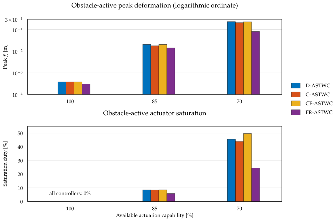
At full capability, no realization saturates, and all formation errors remain at the submillimeter level. D-ASTWC, C-ASTWC, and CF-ASTWC are numerically indistinguishable, while FR-ASTWC introduces a small dynamic-reference transient. This transient raises the active-window mean $\overline{\chi }$ from approximately $0.030$ to $0.162$ mm (a factor of 5.4) and the mean $\overline{\rho }$ from approximately $0.062$ to $0.448$ mm/s (a factor of 7.2). These ratios are disclosed despite the small absolute magnitudes; the reference layer provides no practically meaningful advantage when every follower can realize the demand.

At the marginal 85% regime, FR-ASTWC reduces active peak deformation by 20.3% relative to C-ASTWC and 30.0% relative to CF-ASTWC. At 70%, the separation is larger: relative to C-ASTWC, FR-ASTWC reduces the full-horizon neighbor RMSE, plant saturation duty, and applied control demand by 56.4%, 48.2%, and 11.7%; relative to CF-ASTWC, the reductions are 61.1%, 54.3%, and 12.9%. Table 8 reports the underlying values rather than only percentages.

Table 8. Overall formation and feasibility results over the complete 40 s horizon. “Upstream sat.” denotes common CF/FR filter limiter activity. Effort has units m²/s³.

Capability	Controller	Leader RMSE [m]	Neighbor RMSE [m]	$\mathit{\chi }$ RMSE [m]	Applied Effort	Peak Command [m/s2]	Plant Sat. [%]	Upstream Sat. [%]	Max. Ref. Excursion [m]
100%	D-ASTWC	0.000101	0.000142	0.000107	58.565	2.520	0	0	0
	C-ASTWC	0.000101	0.000141	0.000107	58.564	2.520	0	0	0
	CF-ASTWC	0.000101	0.000142	0.000108	58.564	2.520	0	0	0
	FR-ASTWC	0.000174	0.000113	0.000110	58.643	2.522	0	0	0.00061
85%	D-ASTWC	0.003450	0.004879	0.003702	59.495	5.353	1.272	0	0
	C-ASTWC	0.003109	0.004397	0.003336	59.414	5.423	1.267	0	0
	CF-ASTWC	0.003563	0.005039	0.003823	59.529	5.580	1.277	1.628	0
	FR-ASTWC	0.003220	0.004217	0.003246	58.724	4.644	0.868	1.698	0.01959
70%	D-ASTWC	0.060006	0.082252	0.062757	66.917	8.220	7.403	0	0
	C-ASTWC	0.053216	0.072908	0.055633	66.204	8.643	7.085	0	0
	CF-ASTWC	0.059948	0.081750	0.062434	67.141	9.285	8.033	7.121	0
	FR-ASTWC	0.032746	0.031764	0.026377	58.480	6.958	3.668	7.261	0.16337

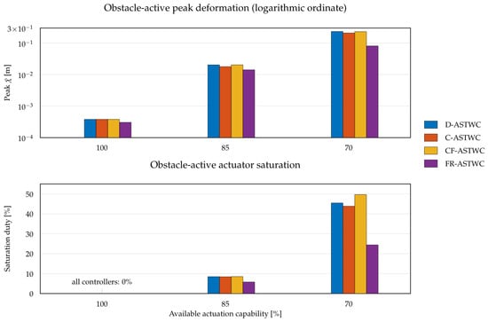
Figure 7 compares the active peak deformation and plant saturation duty with capability ordered from 100% to 70%.

Figure 7. Obstacle-active peak mean formation deformation and plant saturation duty across the capability sweep. The horizontal order follows decreasing available capability: 100%, 85%, and 70%. The corresponding follower-specific final and upstream limits are listed in Table 5. The upper panel uses a logarithmic ordinate so that the submillimeter 100% values remain visible; the lower-panel annotation records that plant saturation duty is exactly zero for every controller at 100%.

7.3. Active Obstacle Transition Response

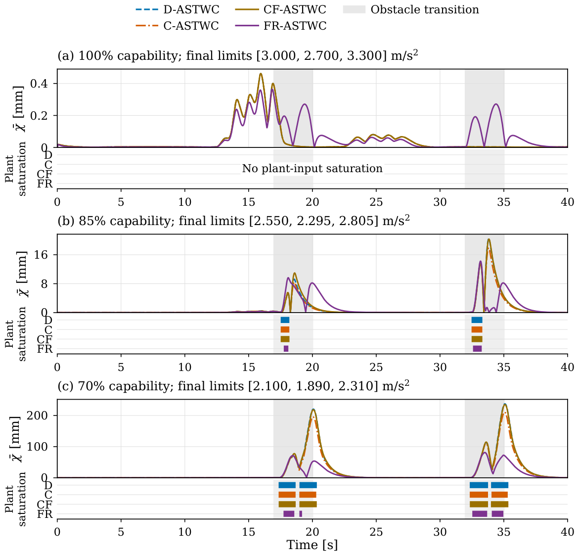
During the acceleration-producing intervals $T_{o,a}$, reference placement provides clearer separation than full-horizon averages. At 85% capability, FR-ASTWC relative to C-ASTWC reduces the peak and mean $\overline{\chi }$ by 20.3% and 19.5%; relative to CF-ASTWC, the reductions are 30.0% and 30.6%. At 70%, the respective peak reductions are 61.1% and 64.9%, and plant saturation exposure falls by 44.3% and 50.8%. For the CF comparison, the absolute active peak changes from 0.23125 to 0.08124 m, the active-window mean from 0.06647 to 0.03441 m (48.2%), and duty from 49.656% to 24.439%. The last change is 25.217 percentage points, or a 50.8% relative reduction. The extended mean (104) exposes the recovery trade-off: at 85%, FR-ASTWC is 1.1% above CF-ASTWC and 17.9% above C-ASTWC, so the active-window mean advantage does not persist through the longer window. At 70%, FR-ASTWC remains 56.8% below CF-ASTWC and 51.5% below C-ASTWC on the extended mean. Table 9 and Table 10 include the 100% active-window baseline as well as the constrained cases.

Table 9. Formation response during obstacle transitions. The active statistics use $[17,20]\cup [32,35]$ s; ${\overline{\chi }}_{\mathrm{ext}}$ uses $[17,23]\cup [32,38]$ s to test sensitivity to the recovery window.

Capability	Controller	Peak $\overline{\mathit{\chi }}$ [m]	Active Mean $\overline{\mathit{\chi }}$ [m]	${\overline{\mathit{\chi }}}_{\mathbf{ext}}$ [m]	Peak/Mean $\overline{\mathit{\rho }}$ [m/s]
100%	D-ASTWC	0.000381	0.000030	0.000017	0.000595/0.000062
	C-ASTWC	0.000381	0.000030	0.000017	0.000595/0.000062
	CF-ASTWC	0.000382	0.000030	0.000017	0.000597/0.000062
	FR-ASTWC	0.000313	0.000162	0.000102	0.000946/0.000448
85%	D-ASTWC	0.02044	0.005733	0.003225	0.12720/0.01963
	C-ASTWC	0.01787	0.005215	0.002920	0.11908/0.01840
	CF-ASTWC	0.02034	0.006046	0.003405	0.12542/0.02039
	FR-ASTWC	0.01424	0.004196	0.003444	0.06533/0.01785
70%	D-ASTWC	0.23375	0.06658	0.06649	0.58118/0.26853
	C-ASTWC	0.20874	0.06160	0.05942	0.52477/0.24860
	CF-ASTWC	0.23125	0.06647	0.06663	0.58474/0.26839
	FR-ASTWC	0.08124	0.03441	0.02880	0.26924/0.13276

Table 10. Actuation and recovery response during active obstacle transition intervals. “Upstream sat.” denotes common CF/FR filter limiter activity; effort has units m²/s³.

Capability	Controller	Applied Effort	Peak Command [m/s2]	Plant Sat. [%]	Upstream Sat. [%]	${\mathit{T}}_{\mathbf{rec},\overline{\mathit{\chi }}}$ [s]	${\mathit{T}}_{\mathbf{rec},\overline{\mathit{\rho }}}$ [s]
100%	D-ASTWC	47.553	2.520	0	0	0	0
	C-ASTWC	47.553	2.520	0	0	0	0
	CF-ASTWC	47.553	2.520	0	0	0	0
	FR-ASTWC	47.636	2.522	0	0	0	0.030
85%	D-ASTWC	48.483	5.353	8.472	0	0.040	0
	C-ASTWC	48.402	5.423	8.439	0	0.026	0
	CF-ASTWC	48.516	5.580	8.505	10.848	0.052	0
	FR-ASTWC	47.717	4.644	5.785	11.315	1.048	0
70%	D-ASTWC	52.819	8.220	45.436	0	1.360	0.678
	C-ASTWC	52.566	8.643	43.860	0	1.334	0.600
	CF-ASTWC	53.121	9.285	49.656	47.446	1.376	0.650
	FR-ASTWC	47.276	6.958	24.439	48.379	1.508	0.044

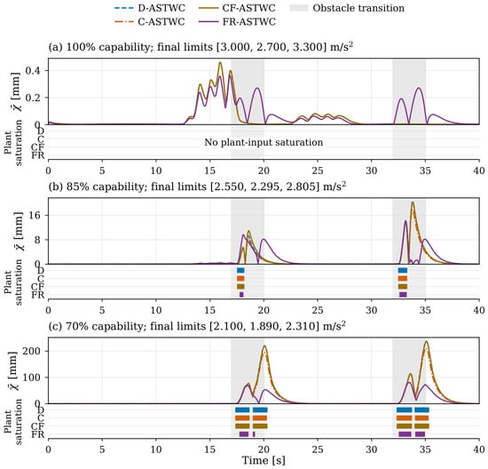
Figure 8 shows the corresponding deformation histories and makes clear that the FR difference is associated with the two acceleration-producing transitions.

Figure 8. Nominal mean weighted deformation and actual plant saturation activity at 100%, 85%, and 70% capability. Gray vertical bands mark the planned transitions $[17,20]\cup [32,35]$ s, not saturation. Controller activity strips are derived from saved follower saturation flags; a colored strip marks samples at which at least one follower is saturated. Strip colors match the controller legend. These strips show temporal activity; the duty statistic separately counts all follower–time samples. Final acceleration limits are identified for each capability; CF/FR upstream limits are 0.90 times these values.

7.4. Robustness Across Bypass Directions and Disturbance Phases

The six-scenario ensemble confirms that the reference placement result is not tied to one lateral direction or favorable disturbance phase. FR-ASTWC has lower peak and mean deformation and plant saturation duty than C-ASTWC and CF-ASTWC in every run. Relative to C-ASTWC, the mean paired reductions are 55.1% in peak $\overline{\chi }$, 41.1% in mean $\overline{\chi }$, and 40.4% in plant saturation. Relative to CF-ASTWC, they are 59.3%, 45.0%, and 47.2%. Table 11 gives the controller-wise ranges.

Table 11. Mean [minimum–maximum] active-interval performance across two bypass directions and three disturbance phase variants at 70% capability.

Controller	Peak $\overline{\mathit{\chi }}$ [m]	Mean $\overline{\mathit{\chi }}$ [m]	Peak $\overline{\mathit{\rho }}$ [m/s]	Plant Sat. [%]	Applied Effort	Commanded Effort
D-ASTWC	0.23450 [0.23375–0.23650]	0.06738 [0.06657–0.06844]	0.59769 [0.58118–0.61521]	47.62 [45.36–50.29]	54.56 [52.79–56.55]	253.25 [237.61–270.60]
C-ASTWC	0.21100 [0.20874–0.21389]	0.06254 [0.06160–0.06368]	0.54319 [0.52477–0.56366]	46.02 [43.78–48.35]	54.22 [52.53–56.10]	267.10 [250.95–285.02]
CF-ASTWC	0.23252 [0.23125–0.23481]	0.06703 [0.06647–0.06787]	0.60682 [0.58474–0.63083]	51.93 [49.58–55.09]	54.90 [53.09–56.93]	268.81 [252.64–286.80]
FR-ASTWC	0.09479 [0.08124–0.10985]	0.03686 [0.03441–0.03945]	0.30768 [0.26924–0.34820]	27.52 [24.36–30.75]	48.78 [47.25–50.53]	104.39 [89.25–121.90]

For each metric in Table 12, the percentage reduction is computed within each matched scenario before its mean and range are taken. This avoids ratios of aggregate means.

Table 12. Paired FR-ASTWC reductions across the six scenario variants; entries are mean [minimum–maximum].

Comparison	Peak $\overline{\mathit{\chi }}$ Reduction [%]	Mean $\overline{\mathit{\chi }}$ Reduction [%]	Plant Saturation Reduction [%]
FR-ASTWC vs. C-ASTWC	55.1 [48.3–61.1]	41.1 [37.6–44.2]	40.4 [36.4–44.4]
FR-ASTWC vs. CF-ASTWC	59.3 [52.8–64.9]	45.0 [41.3–48.3]	47.2 [43.2–50.9]

Using aggregate means, FR-ASTWC also reduces the peak $\overline{\rho }$, applied control demand, and commanded control demand relative to CF-ASTWC by 49.3%, 11.2%, and 61.2%. The negative-y bypass is more demanding, but the performance ordering does not change. Because Table 11 reports minima across six variants, a minimum need not equal the positive-y reference-run value in Table 9; all displayed values are rounded independently from the underlying unrounded runs. These scenario statistics support repeatability within the tested family; they are not inferential population statistics. Table 13 lists the individual scenario results.

Table 13. Individual deterministic scenarios at 70% capability. Phase offsets are in radians; reductions are paired CF-to-FR percentages. Their arithmetic means recover 59.3%, 45.0%, and 47.2%.

Scenario	Bypass	$(\Delta {\mathit{\varphi }}_1,\Delta {\mathit{\varphi }}_2)$	CF Peak [m]	FR Peak [m]	Peak Reduction [%]	Active Mean Reduction [%]	Duty Reduction [%]
S001	$+y$	$(0.00,0.00)$	0.23125	0.08124	64.87	48.23	50.78
S002	$+y$	$(0.37,-0.29)$	0.23125	0.08124	64.87	48.27	50.64
S003	$+y$	$(-0.41,0.33)$	0.23125	0.08124	64.87	48.24	50.86
S004	$-y$	$(0.00,0.00)$	0.23250	0.10985	52.75	41.30	44.18
S005	$-y$	$(0.37,-0.29)$	0.23481	0.10742	54.25	42.25	43.29
S006	$-y$	$(-0.41,0.33)$	0.23402	0.10774	53.96	41.86	43.17

7.5. Safety Margins, Reference Excursion, and Recovery

For the reference positive-y scenario at 70% capability, the common preplanned path preserves a positive required obstacle margin of approximately 0.45 m for every realization. These nearly identical obstacle margins are dominated by the external path geometry and must not be interpreted as controller-level safety superiority. The positive inter-UAV values likewise demonstrate only numerical feasibility for this scenario. The maximum FR reference excursion is 0.1634 m, showing that reduced physical deformation is obtained by permitting a bounded temporary departure of the commanded follower reference from the nominal leader offset.

The recovery-time effect is signal-dependent. FR-ASTWC crosses the $\overline{\chi }$ recovery threshold later than C-ASTWC and CF-ASTWC because the anchored reference returns smoothly, but its $\overline{\rho }$ recovery is faster. The paper therefore does not claim uniformly faster recovery or improved disturbance window rejection.

For $y\in \{\overline{\chi },\overline{\rho }\}$, let $y_{\mathrm{pre}}$ be its sampled mean over $[12,17)$ s preceding the first transition, and let $y_{\mathrm{pk}}$ be its peak over $[17,35]$ s. Define $y_{\mathrm{th}}=y_{\mathrm{pre}}+0.2(y_{\mathrm{pk}}-y_{\mathrm{pre}})$, and let $t_y^{\star }\ge 35$ s be the first sampled time at which every sampled value of y through $t_y^{\star }+0.5$ s is at or below $y_{\mathrm{th}}$. The implementation floors $y_{\mathrm{pk}}-y_{\mathrm{pre}}$ at ${10}^{-12}$ in the corresponding signal units; this does not affect the reported recovery values. The recovery time is the elapsed delay $T_{\mathrm{rec},\mathrm{y}}=t_y^{\star }-35\mathrm{s}$. The reported safety margins are

$$\begin{array}{cc}\hfill m_{\mathrm{obs}}& =\underset{i,t}{\min }\left[∥p_i\left(t\right)-p_o∥-(R_o+R_i+d_{\mathrm{req}})\right],\hfill \\ \hfill m_{\mathrm{pair}}& =\underset{i<j,t}{\min }\left[∥p_i\left(t\right)-p_j\left(t\right)∥-(R_i+R_j+d_{\mathrm{sep}})\right].\hfill \end{array}$$

(106)

Table 14 reports these geometry, reference, and recovery indicators.

Table 14. Selected safety, reference, and recovery indicators for the reference positive-y scenario at 70% capability.

Metric	D-ASTWC	C-ASTWC	CF-ASTWC	FR-ASTWC
Minimum required obstacle margin [m]	0.45000	0.45000	0.45000	0.45007
Minimum inter-UAV safety margin [m]	1.30039	1.32502	1.30148	1.45410
Maximum reference excursion [m]	0	0	0	0.16337
$T_{\mathrm{rec},\overline{\chi }}$ [s]	1.360	1.334	1.376	1.508
$T_{\mathrm{rec},\overline{\rho }}$ [s]	0.678	0.600	0.650	0.044

7.6. Sensitivity to Cue, Anchor, and Reference Limit Settings

All 144 sensitivity simulations were completed with finite states and commands, positive sampled clearance margins, and a qualifying recovery hold before the horizon ended. Table 15 summarizes the local gain sweeps. At 70%, the nominal and $\pm 25\%$ cue/anchor variants retain CF-to-FR reductions of 63.1–65.2% in active peak deformation, 46.6–49.6% in the active-window mean, and 49.2–52.4% in the plant saturation duty. These ranges indicate local insensitivity to the selected gain perturbations; they are not an admissible tuning-domain proof.

Table 15. Ranges of paired percentage reductions relative to CF over each nominal/$\pm 25\%$ gain sweep. Positive values favor FR; negative values denote deterioration. The last column deliberately reports the 85% extended-window trade-off.

Varied Gain Group	Peak, 70%	Active Mean, 70%	Plant Duty, 70%	Extended Mean, 85%
Proportional cue $K_{p,f,i}$	$[64.6,65.1]$	$[47.1,49.2]$	$[49.8,51.8]$	$[-5.5,2.8]$
Derivative cue $K_{d,f,i}$	$[64.9,65.0]$	$[47.2,49.1]$	$[50.0,51.4]$	$[-1.2,-1.0]$
Proportional anchor $k_{n,p}$	$[63.1,64.9]$	$[46.6,49.6]$	$[49.2,52.4]$	$[-3.9,1.3]$
Derivative anchor $k_{n,v}$	$[64.6,65.2]$	$[47.5,48.8]$	$[49.7,52.3]$	$[-2.5,0.5]$

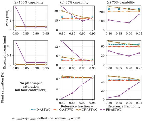
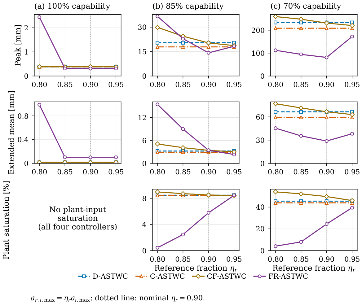
The upstream/final limit ratio has a stronger, nonmonotone effect (Figure 9). At 70%, reducing the ratio from 0.90 to 0.80 lowers FR plant duty from 24.44% to 4.13% but increases its active peak from 0.08124 to 0.11243 m and its active-window mean from 0.03441 to 0.05016 m. Raising it to 0.95 instead increases the peak to 0.17245 m and duty to 39.45%. A smaller upstream demand therefore does not by itself imply a smaller formation error.

Figure 9. Sensitivity to the common CF/FR upstream-to-final acceleration limit ratio ${\eta }_r=a_{r,i,\max }/a_{i,\max }$. Only this ratio changes; all other parameters remain nominal. Peak and extended-window mean deformation are shown with plant saturation duty, exposing the trade-off between reference restriction and plant demand. These are deterministic local tests.

At 85% with ratio 0.80, FR has an active peak of 0.03663 m versus CF’s 0.02989 m, and the extended-window means are 0.01546 and 0.00508 m, respectively. With ratio 0.95, FR’s plant duty is slightly higher than CF’s (8.450% versus 8.428%), despite having lower deformation means. Across all 12 settings at 85%, FR has a worse extended-window mean than CF in eight settings. At 100%, plant saturation remains absent, but the 0.80 ratio produces a 2.442 mm FR peak; the submillimeter statement for the nominal full-capability case does not apply to this altered setting. Recovery is also metric-dependent: FR’s deformation recovery is slower than CF’s in 11 of 12 settings at both 70% and 85%. Thus, 0.90 is retained as the original compromise and is not asserted to be universally optimal.

7.7. Paired Monte Carlo Validation

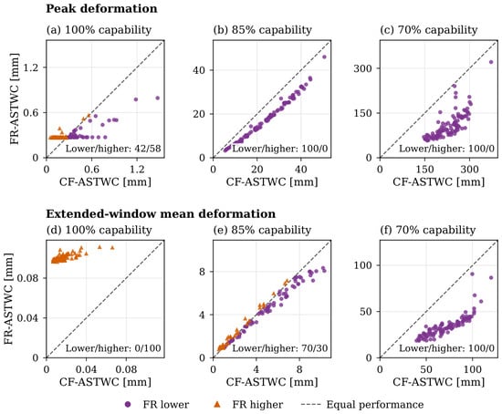
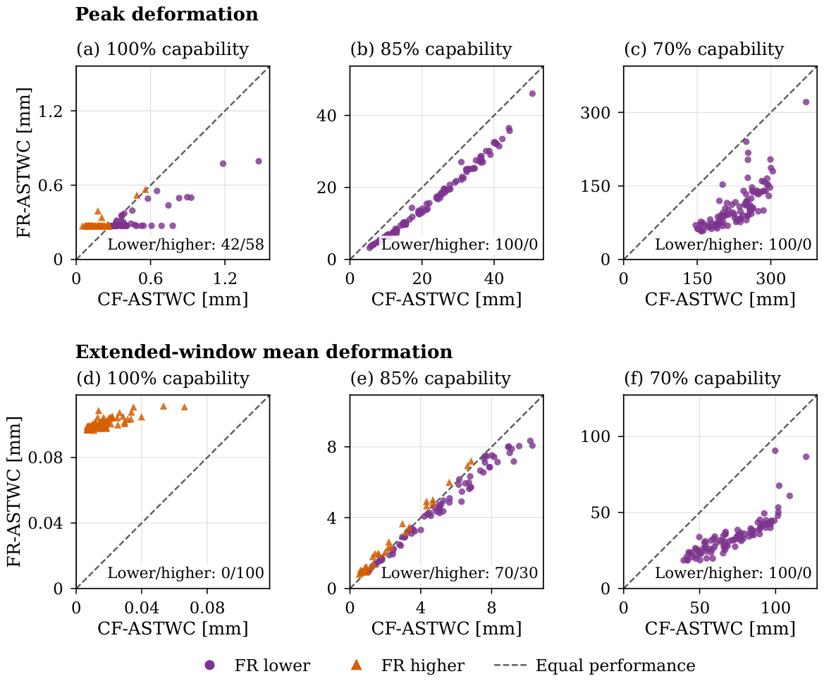
All 1200 simulations were completed: 100 matched scenarios per capability, with no execution failures or missing controller pairs. The draw contained 48 positive-y and 52 negative-y bypasses. No negative sampled obstacle/inter-UAV margins or unobserved recovery holds occurred; the all-run minimum margins were 0.35004 and 1.20178 m. These finite-horizon observations do not constitute safety or global stability guarantees. Table 16 reports the absolute performance and paired intervals, and Figure 10 exposes the individual CF/FR pairs.

Table 16. Paired Monte Carlo comparison with CF-ASTWC, 100 complete scenarios per capability. Controller values are mean ± sample standard deviation. The improvement column gives the mean absolute CF-minus-FR difference and its 95% percentile bootstrap interval; units are mm for deformation and percentage points for duty. Positive differences favor FR. “Better” counts strictly improved pairs; the 100% duty case has 100 ties.

Capability	Metric	CF	FR	Improvement [95% Interval]	FR Better
70%	Peak [mm]	$231.72\pm 44.33$	$109.09\pm 43.65$	122.63 [116.36, 128.61]	100/100
70%	Active mean [mm]	$71.99\pm 16.70$	$41.61\pm 15.78$	30.38 [29.48, 31.24]	100/100
70%	Extended mean [mm]	$71.99\pm 18.76$	$34.38\pm 11.98$	37.61 [35.42, 39.70]	100/100
70%	Plant duty [%]	$50.65\pm 7.64$	$26.80\pm 4.57$	23.85 [22.75, 24.93]	100/100
85%	Peak [mm]	$23.50\pm 11.25$	$17.22\pm 9.52$	6.28 [5.87, 6.67]	100/100
85%	Active mean [mm]	$7.65\pm 4.58$	$5.12\pm 2.87$	2.53 [2.19, 2.88]	97/100
85%	Extended mean [mm]	$4.38\pm 2.70$	$4.06\pm 2.30$	0.32 [0.21, 0.44]	70/100
85%	Plant duty [%]	$8.78\pm 2.01$	$6.11\pm 1.41$	2.67 [2.51, 2.84]	100/100
100%	Peak [mm]	$0.311\pm 0.240$	$0.309\pm 0.096$	0.003 [–0.032, 0.039]	42/100
100%	Active mean [mm]	$0.028\pm 0.019$	$0.160\pm 0.006$	–0.132 [–0.134, –0.129]	0/100
100%	Extended mean [mm]	$0.016\pm 0.009$	$0.101\pm 0.003$	–0.085 [–0.086, –0.083]	0/100
100%	Plant duty [%]	$0.00\pm 0.00$	$0.00\pm 0.00$	0.00 [0.00, 0.00]	0/100

Figure 10. Paired CF/FR Monte Carlo outcomes for active peak and extended-window mean deformation at each capability. Each point represents the same sampled scenario evaluated by both controllers; the diagonal denotes equality. Points below the diagonal favor FR. Axis scales differ by capability to resolve the small full-capability errors.

At 70%, FR improves all three primary endpoints relative to each of D, C, and CF in every draw. Against CF, the mean paired percentage reductions are 53.8% (95% interval 51.4–56.1%) for the active peak, 43.4% (41.9–44.9%) for the active-window mean, and 46.7% (45.3–48.1%) for the plant saturation duty. The absolute CF/FR means are 0.23172/0.10909 m, 0.07199/0.04161 m, and 50.65/26.80%, respectively. Nevertheless, one draw (S071) has a higher FR full-horizon leader RMSE than all three alternatives, a higher neighbor RMSE than C and CF, and a higher extended-window mean than C. A primary active-window improvement does not imply an improvement in every metric in every realization.

At 85%, FR improves the CF active peak and plant duty in all 100 draws, as well as the active-window mean in 97. The extended-window mean improves in 70 draws and worsens in 30. Its mean paired percentage reduction is 1.2%, with a 95% interval of $[-2.4,4.5]\%$. The mean absolute difference is positive (0.319 mm, interval 0.206–0.437 mm); this is a different estimand because percentages weight small baselines more strongly. Against C, the extended-window mean worsens in 79 draws, with a mean paired reduction of $-13.6\%$ (interval $[-18.3,-9.5]\%$). These results support a peak/saturation advantage but not a uniform recovery window advantage. FR deformation recovery is slower than CF in 99 of the 100 draws at 85%; at 70%, it is slower in 55, faster in 43, and tied in two, despite a lower mean delay. The maximum FR reference excursion across all draws is 0.2794 m, compared with 0.1634 m in the nominal 70% case.

At 100%, all controllers remain unsaturated. The nominal submillimeter statement is not a bound for every perturbed case; the largest CF active peak in the Monte Carlo draws is 1.473 mm. The mean active peaks for CF and FR are 0.311 and 0.309 mm; the paired absolute-difference interval includes zero, and FR has a larger peak in 58 draws. Its active- and extended-window means are larger in all 100 draws. Because the individual baseline errors are very small, the relative percentages can be large or rank differently from the difference in means; absolute values are therefore emphasized. The Monte Carlo study corroborates the restrictive capability trend within the declared uncertainty design, while retaining the low-demand and recovery trade-offs.

8. Discussion

8.1. Dynamic Filtering Versus Reference Placement

The nominal sweep supports a conditional architectural claim. At 100% capability, the absolute deformation remains submillimeter, and no controller saturates, although FR-ASTWC’s anchored transient produces larger active-window means than the other realizations. At 85%, all final plant limits exceed the planned peak lateral acceleration, yet follower 2 has little nominal headroom and the upstream filter becomes active. FR-ASTWC lowers peak and active-window deformation relative to both input placements, but its extended-window mean is slightly above those of CF-ASTWC and C-ASTWC because the anchored reference returns more slowly. At 70%, followers 1 and 2 cannot reproduce the leader’s peak lateral acceleration from feedforward alone, and FR-ASTWC retains a 56.8% extended-window mean reduction relative to CF-ASTWC. Thus, the 85% benefit is limited to peak/active transition behavior and reduced saturation, whereas the broader mean deformation advantage is supported in the tighter 70% regime.

CF-ASTWC is the decisive ablation because it uses the same anchored second-order filter and limit as FR-ASTWC. Its poorer response in the nominal constrained cases shows that smoothing and amplitude limiting alone do not reproduce the observed FR benefit when the nominal target remains unchanged and the filtered cue is still injected at the plant input. FR-ASTWC instead makes $p_{r,i},v_{r,i},a_{r,i}$ the tracked target. Proposition 1 provides the parallel theoretical distinction: FR preserves ${\delta }_i={\vartheta }_i$, while CF adds the filtered cue to the inner residual. This residual topology, not higher gains or extra plant capability, is the structural distinction of reference placement.

The price of this behavior is a temporary reference displacement. The 0.1634 m maximum excursion is not a hidden tracking failure; it is the mechanism by which the architecture replaces an infeasible instantaneous formation demand with an anchored, acceleration-limited target. FR-ASTWC does not create additional physical capability.

8.2. Robustness to Bypass Direction and Disturbance Phase

The six-scenario ensemble broadens the evidence beyond one favorable trajectory. The negative-y bypass increases deformation and saturation for every controller, whereas phase changes produce smaller variation. FR-ASTWC remains better than C-ASTWC and CF-ASTWC on the three paired primary metrics in every run. The reported ranges support repeatability for this scenario family, not distribution-free robustness or statistical generalization.

The additional Monte Carlo study broadens the tested family to drag mismatch, actuation variation, disturbance variation, and initial offsets, while retaining the paired comparisons. Its 70% gains coexist with unfavorable secondary metrics and 85% recovery window trade-offs. Both studies still use one obstacle size, one formation shape, three followers, and a fixed complete graph; neither proves scalability or topology-independent performance.

8.3. Disturbance Rejection and Formation Management

The directionally heterogeneous matched disturbances are handled by the common adaptive super-twisting tracker. The reference filter uses only ${\chi }_i$ and ${\dot{\chi }}_i$ and does not insert an observer estimate into the commanded trajectory. The Monte Carlo experiment perturbs disturbances jointly with other quantities; it does not isolate an improvement in disturbance rejection. The evidenced advantage concerns formation demand management during obstacle transitions.

The graph-theoretic identity (31) shows that the collection of local deformation vectors bounds the global formation error. No controller reallocates thrust between vehicles, and a follower cannot donate actuation capability to another follower. The mechanism remains distributed coupled error feedback.

8.4. Control Demand Integral

Across the six 70% capability variants, FR-ASTWC reduces the mean active-window applied and commanded control demand integrals by 11.2% and 61.2% relative to CF-ASTWC. The reduction is consistent with shorter exposure to the final plant limit and a smaller unsaturated command.

Nevertheless,

$$J_{u,a}={\int }_{T_{o,a}}{\displaystyle \sum _{i=1}^N}{∥u_i\left(t\right)∥}^{2}dt$$

(107)

is not electrical energy. Battery energy depends on rotor thrust, induced and profile power, motor efficiency, vehicle velocity, and hover consumption. The present study therefore reports a control demand integral only; no battery saving conclusion is drawn.

8.5. Certificate Scope and Practical Implementation

The common quadratic certificate is strict for the ideal D/FR residuals of all three followers. It neither certifies arbitrary saturation transients nor C/CF cue derivatives. The printed reaching coefficients are deliberately reported as conservative Lyapunov bounds and are not presented as predictions of the simulated recovery times. Proposition 2 is conditional on bounded implemented residuals, which are observed on the finite horizon rather than proven globally.

The projected gain scheduler is identical in all four cases and prevents the gain law from being a hidden comparison variable. No fixed-gain ablation is included, so the numerical results do not establish that adaptation itself is necessary for the observed benefit; the paper’s claim concerns placement. Likewise, ${ϵ}_s={10}^{-3}$ is fixed. The nominal submillimeter 100% residuals are within the expected regularization layer, but a sampling time and ${ϵ}_s$ sensitivity study remains for future work.

For fixed spatial dimensions, evaluating local formation signals costs $O\left(q_i\right)$ operations per follower and $O(N+|{\mathcal{E}}_f\left|\right)$ across the network. CF and FR add six scalar filter/reference states per follower and fixed-size vector operations; neither requires online optimization or matrix inversion. The common quadratic audit is offline. The implementation assumes measured position/velocity, neighbor-relative states, and the broadcast leader acceleration; it requires neither measured acceleration nor numerical differentiation of the deformation cue. Communication delay and controller-only hardware timing are not measured. The recorded simulation times include integration, history storage, and diagnostics and therefore do not establish real-time feasibility.

8.6. Limitations

The plant is a mass-normalized translational outer-loop model with exact drag in the deterministic tests and a declared drag mismatch in the Monte Carlo study. Heterogeneity is dynamically active through ${\beta }_i$ and $a_{i,\max }$, while $m_i$ is a physical descriptor used to recover force and drag; unknown mass, attitude dynamics, motor lag, and unmatched disturbances remain outside the scope of the study. The mixed Monte Carlo perturbations do not isolate the causal contribution of each uncertainty source. The graph is fixed and complete, communication is ideal, and only three followers, one obstacle, and one formation shape are tested. The filter has no separately analyzed anti-windup compensator, recovery is observed only through 40 s, and the clearance values are planner-dominated numerical checks.

No external controller from the literature is benchmarked. The experiment is intentionally an internal matched-implementation placement study, so it cannot support superiority over reference governors, command-filtered backstepping, or recent constrained formation controllers. Hardware experiments; larger sparse formations; formal safety layers; inner gain, sampling time, and regularization sensitivity; and calibrated propulsion energy measurements remain for future work.

9. Conclusions

FR-ASTWC places a local deformation cue in an anchored, acceleration-limited follower reference that is tracked by a common adaptive super-twisting loop. The matched four-controller study distinguishes this placement from direct or dynamically filtered cue insertion at the plant input. In the nominal exact drag model, D and FR retain the exogenous ideal residual. C and CF include a state-dependent cue in this residual and require additional cue derivative bounds for certification. The reported common quadratic certificate concerns ideal D/FR tracking; the practical formation bound remains conditional.

At 70% nominal capability, FR reduces the active peak deformation, active-window mean deformation, and plant saturation duty relative to CF by 64.9%, 48.2%, and 50.8%. The six deterministic scenarios give mean paired reductions of 59.3%, 45.0%, and 47.2%. In 100 paired Monte Carlo draws at the same capability, the corresponding means are 53.8%, 43.4%, and 46.7%, with improvements at all three endpoints in every draw. These findings support reference placement under the tested tight constraints, without establishing superiority over external controllers.

The benefit is conditional on the operating regime, metric, and tuning. At 85%, reduced active peaks can coexist with a worse extended-window mean; at 100%, the dynamic reference transient increases the mean deformation. An overly restrictive upstream limit can also worsen deformation despite reducing plant saturation. The Monte Carlo cases are empirical stress tests outside the asserted nominal certificate. No general collision avoidance, global saturated-system stability, or battery energy guarantee follows. Future work includes formal safety and anti-windup layers, sparse or switching graphs, communication imperfections, inner-loop numerical sensitivity, and experimental multirotor validation.

References

- Olfati-Saber, R.; Fax, J.A.; Murray, R.M. Consensus and cooperation in networked multi-agent systems. Proc. IEEE 2007, 95, 215–233. [Google Scholar] [CrossRef] [Scilit]
- Ren, W.; Beard, R.W. Consensus seeking in multiagent systems under dynamically changing interaction topologies. IEEE Trans. Autom. Control 2005, 50, 655–661. [Google Scholar] [CrossRef] [Scilit]
- Mesbahi, M.; Egerstedt, M. Graph Theoretic Methods in Multiagent Networks; Princeton University Press: Princeton, NJ, USA, 2010. [Google Scholar]
- Oh, K.-K.; Park, M.-C.; Ahn, H.-S. A survey of multi-agent formation control. Automatica 2015, 53, 424–440. [Google Scholar] [CrossRef] [Scilit]
- Bu, Y.; Yan, Y.; Yang, Y. Advancement challenges in UAV swarm formation control: A comprehensive review. Drones 2024, 8, 320. [Google Scholar] [CrossRef] [Scilit]
- Yu, C.; Liu, J.; Xie, P.; Xie, W. A comprehensive review of UAV formation control from a mission-driven perspective. Drones 2026, 10, 278. [Google Scholar] [CrossRef] [Scilit]
- Li, W.; Yan, S.; Shi, L.; Yue, J.; Shi, M.; Lin, B.; Qin, K. Multiagent consensus tracking control over asynchronous cooperation–competition networks. IEEE Trans. Cybern. 2025, 55, 4347–4360. [Google Scholar] [CrossRef] [Scilit]
- Li, W.; Wen, C.; Shi, M.; Qin, K.; Shi, L. On asynchronous bipartite consensus over quasi-structurally balanced signed networks. IEEE Trans. Control Netw. Syst. 2026, early access. [Google Scholar] [CrossRef] [Scilit]
- Dong, X.; Yu, B.; Shi, Z.; Zhong, Y. Time-varying formation control for unmanned aerial vehicles: Theories and applications. IEEE Trans. Control Syst. Technol. 2015, 23, 340–348. [Google Scholar] [CrossRef] [Scilit]
- Liang, Y.; Dong, Q.; Zhao, Y. Adaptive leader–follower formation control for swarms of unmanned aerial vehicles with motion constraints and unknown disturbances. Chin. J. Aeronaut. 2020, 33, 2972–2988. [Google Scholar] [CrossRef] [Scilit]
- Liu, B.; Li, A.; Guo, Y.; Wang, C. Adaptive distributed finite-time formation control for multi-UAVs under input saturation without collisions. Aerosp. Sci. Technol. 2022, 120, 107252. [Google Scholar] [CrossRef] [Scilit]
- Zhou, P.; Chen, B.M. Semi-global leader-following consensus-based formation flight of unmanned aerial vehicles. Chin. J. Aeronaut. 2022, 35, 31–43. [Google Scholar] [CrossRef] [Scilit]
- Liu, H.; Ma, T.; Lewis, F.L.; Wan, Y. Robust formation trajectory tracking control for multiple quadrotors with communication delays. IEEE Trans. Control Syst. Technol. 2020, 28, 2633–2640. [Google Scholar] [CrossRef] [Scilit]
- Yang, W.; Shi, Z.; Zhong, Y. Distributed robust adaptive formation control of multi-agent systems with heterogeneous uncertainties and directed graphs. Automatica 2023, 157, 111275. [Google Scholar] [CrossRef] [Scilit]
- Chang, X.; Yang, Y.; Zhang, Z.; Jiao, J.; Cheng, H.; Fu, W. Consensus-based formation control for heterogeneous multi-agent systems in complex environments. Drones 2025, 9, 175. [Google Scholar] [CrossRef] [Scilit]
- Wang, Z.; Qin, Y.; Tao, F.; Wu, Z.; Gao, S. Cooperative networked quadrotor UAV formation and prescribed time tracking control with speed and input saturation constraints. Drones 2025, 9, 417. [Google Scholar] [CrossRef] [Scilit]
- Bao, G.; Ma, L.; Yi, X. Recent advances on cooperative control of heterogeneous multi-agent systems subject to constraints: A survey. Syst. Sci. Control Eng. 2022, 10, 539–551. [Google Scholar] [CrossRef] [Scilit]
- Li, Y.; Zhao, W.; Zhu, L.; Zhang, Z.; Guo, Y. Fixed-time cooperative formation control of heterogeneous systems under multiple constraints. Entropy 2025, 27, 538. [Google Scholar] [CrossRef] [Scilit]
- Levant, A. Higher-order sliding modes, differentiation and output-feedback control. Int. J. Control 2003, 76, 924–941. [Google Scholar] [CrossRef] [Scilit]
- Moreno, J.A.; Osorio, M. Strict Lyapunov functions for the super-twisting algorithm. IEEE Trans. Autom. Control 2012, 57, 1035–1040. [Google Scholar] [CrossRef] [Scilit]
- Seeber, R.; Horn, M. Stability proof for a well-established super-twisting parameter setting. Automatica 2017, 84, 241–243. [Google Scholar] [CrossRef] [Scilit]
- Shtessel, Y.; Taleb, M.; Plestan, F. A novel adaptive-gain supertwisting sliding mode controller: Methodology and application. Automatica 2012, 48, 759–769. [Google Scholar] [CrossRef] [Scilit]
- Shtessel, Y.; Edwards, C.; Fridman, L.; Levant, A. Sliding Mode Control and Observation; Birkhäuser: New York, NY, USA, 2014. [Google Scholar] [CrossRef] [Scilit]
- Ye, Y.; Hu, S.; Zhu, X.; Sun, Z. An improved super-twisting sliding mode composite control for quadcopter UAV formation. Machines 2024, 12, 32. [Google Scholar] [CrossRef] [Scilit]
- Dou, J.; Wu, Y.; Xie, D.; Zhang, T. Trajectory tracking and formation control of quadrotor UAVs based on modified super twisting sliding mode method. Sci. Rep. 2025, 15, 24039. [Google Scholar] [CrossRef] [Scilit]
- Garone, E.; Di Cairano, S.; Kolmanovsky, I.V. Reference and command governors for systems with constraints: A survey on theory and applications. Automatica 2017, 75, 306–328. [Google Scholar] [CrossRef] [Scilit]
- Nicotra, M.M.; Bartulovic, M.; Garone, E.; Sinopoli, B. A distributed explicit reference governor for constrained control of multiple UAVs. IFAC-PapersOnLine 2015, 48, 156–161. [Google Scholar] [CrossRef] [Scilit]
- Convens, B.; Merckaert, K.; Vanderborght, B.; Nicotra, M.M. Invariant set distributed explicit reference governors for provably safe on-board control of nano-quadrotor swarms. Front. Robot. AI 2021, 8, 663809. [Google Scholar] [CrossRef] [Scilit]
- Farrell, J.A.; Polycarpou, M.; Sharma, M.; Dong, W. Command filtered backstepping. IEEE Trans. Autom. Control 2009, 54, 1391–1395. [Google Scholar] [CrossRef] [Scilit]
- Mellinger, D.; Kumar, V. Minimum snap trajectory generation and control for quadrotors. In Proceedings of the 2011 IEEE International Conference on Robotics and Automation, Shanghai, China, 9–13 May 2011; pp. 2520–2525. [Google Scholar] [CrossRef] [Scilit]
- Hönig, W.; Preiss, J.A.; Kumar, T.K.S.; Sukhatme, G.S.; Ayanian, N. Trajectory planning for quadrotor swarms. IEEE Trans. Robot. 2018, 34, 856–869. [Google Scholar] [CrossRef] [Scilit]
- Zhang, P.; Wang, Z.; Zhu, Z.; Liang, Q.; Luo, J. Enhanced multi-UAV formation control and obstacle avoidance using IAAPF-SMC. Drones 2024, 8, 514. [Google Scholar] [CrossRef] [Scilit]
- Li, Y.; Zhang, P.; Wang, Z.; Rong, D.; Niu, M.; Liu, C. Multi-UAV obstacle avoidance and formation control in unknown environments. Drones 2024, 8, 714. [Google Scholar] [CrossRef] [Scilit]
- Choi, J.; Choi, Y. Development of a bearing-based distributed control method for UAV formation tracking and obstacle avoidance. Aerospace 2025, 12, 1013. [Google Scholar] [CrossRef] [Scilit]
- Feng, X.; Cheng, H.; Wang, H.; Xie, X.; Wei, W.; Han, T.; Liu, S. Capability-aware hierarchical control with priority-based lateral recovery for deadline-guided fixed-wing UAV formation tracking. Drones 2026, 10, 530. [Google Scholar] [CrossRef] [Scilit]
- Boyd, S.; El Ghaoui, L.; Feron, E.; Balakrishnan, V. Linear Matrix Inequalities in System and Control Theory; SIAM: Philadelphia, PA, USA, 1994. [Google Scholar]
- Khalil, H.K. Nonlinear Systems, 3rd ed.; Prentice Hall: Upper Saddle River, NJ, USA, 2002. [Google Scholar]
Disclaimer/Publisher’s Note: The statements, opinions and data contained in all publications are solely those of the individual author(s) and contributor(s) and not of MDPI and/or the editor(s). MDPI and/or the editor(s) disclaim responsibility for any injury to people or property resulting from any ideas, methods, instructions or products referred to in the content. |
© 2026 by the author. Licensee MDPI, Basel, Switzerland. This article is an open access article distributed under the terms and conditions of the Creative Commons Attribution (CC BY) license.