Low-Cost Fixed Bi-Rotor Testbed for Experimental Testing of Linear and Nonlinear Controllers

Abstract

To build a comprehensive academic or scientific foundation in control theory, developing the theoretical foundation is essential; however, it is equally crucial to validate the theory through practical or experimental verification. Therefore, it is necessary to have platforms that support the learning of automatic control theory. This paper proposes a fixed bi-rotor testbed as an educational tool to help undergraduate and graduate students verify control theories related to electronic engineering and automatic control systems. To evaluate the performance of the fixed bi-rotor testbed, three linear control laws are introduced: Proportional (P), Proportional Derivative (PD), and Proportional Integral Derivative (PID). Additionally, three nonlinear control techniques are examined: Backstepping, Nested Saturations, and First-Order Sliding Modes (SMC). The linear and nonlinear controller gains have been adjusted through several heuristic experiments. In multiple tests, the PD and backstepping control laws performed better than the other control techniques on the fixed bi-rotor testbed.

1. Introduction

The development of control theory is crucial to science. Platforms and testbeds are widely used in research, education, and academic training in control theory. However, it is also essential to have low-cost platforms that support experimental verification of these theories and promote learning and educational training at both undergraduate and graduate levels in universities and research centers.

Thus, the platforms described in this brief state of the art comprise actuated and sub-actuated systems. Below, we present some works on testbeds used to apply automatic control theory.

It should be mentioned that the development of commercial platforms or those created by industry is not included in this brief overview due to their high economic costs. For this work, we focus on prototype control theory platforms designed and built by universities and research centers.

In [1], a prototype bipedal robot is introduced, designed to improve fundamental understanding of controlled legged locomotion. It was developed as the simplest mechanical structure that still appropriately represents human walking. The need for mechanical simplicity naturally limited its motion to the sagittal plane, with lateral stabilization achieved through external means. The motivation for studying walking robots, as shown in [1], stems from various social and commercial interests, including the goal of replacing humans in dangerous jobs, such as inspecting nuclear power plants and conducting military operations and medical therapy. Furthermore, [1] considers the production of bipedal toys that help spark or revive interest in robotics among younger audiences.

On the other hand, in [2], a platform is presented that primarily measures the output torque of an actuator or motor. This actuator is designed for use in a gyroscope for posture control and to verify gyroscopic theory quickly and simply. The goal is to teach the fundamentals of automatic control and the operation of gyroscopes. The method also allows for testing and validation in thermal and vacuum environments.

In [3], a quadrotor testbed was created to allow safe verification of the developed algorithms at a ground station before conducting real-time flights. Subsequently, a flight control strategy and a trajectory generation method, both of which are conceptually and computationally lightweight, were developed and tested in a simulation environment. After the simulations, both a real-time experimental environment and a simulation environment were established and connected to the actual system.

Since all experimental platforms for testing automatic control theories comprise both software and hardware,  [4] presents a low-cost platform that addresses various issues in practical automatic control work. The testbed in [4] is designed to apply linear control laws in the position and velocity of continuous-current motors.

Another affordable platform that yields optimal experimental results is based on the popular Arduino Mega microcontroller, along with a power stage and a Hall-effect detection stage. This testbed is discussed in [5], which also includes a magnetic levitation test bench. This test bench has helped many students demonstrate and understand nonlinear effects in electromagnetic field theory and automatic control theory.

A fundamental part of developing platforms for conducting automatic control experiments is reducing costs and risks when implementing a control law on a larger vehicle, such as an F/A-18A aircraft or a space module, as presented in [6], in which they develop a platform to test control algorithms for launch vehicles and for the landing system of aerial vehicles. The prototype they propose is a four-rotor drone with an inverted flexible pendulum at its top and another simple pendulum at its bottom. The aim is to test external disturbances on the vehicle during takeoff and landing before implementing them on the larger vehicle that will perform the assigned tasks [6].

On the other hand, the self-balancing robot (SBR), also known as a two-wheeled inverted pendulum, is a highly nonlinear mechanical system that is of great interest in automatic control research. Although some SBR systems are commercially available, most lack the features needed for control experiments; consequently, many studies rely on locally developed prototypes.

The typical configuration of an SBR consists of an inverted pendulum mounted on a differential platform with only two wheels on the same axis. Examples of this setup can be found in [7], where an Arduino Mega development board is used to control the system, and in [8], where an STM32F103C8T6 development board is used. In [7,8], the entire control algorithm runs on the microcontroller onboard the robot.

In [9], a self-balancing robot (SBR) is built using an Arduino Mega for basic tasks, including actuator control and sensor data acquisition. It is paired with a Raspberry Pi 4 single-board computer, which manages image capture and analysis, and communicates with a desktop PC running MATLAB to send path commands. In [7,8,9], the wheels are powered by DC motors with encoders controlled through H-bridge drivers, while inertia measurement units measure the pendulum angle.

In [10], a larger prototype is shown, equipped with an embedded industrial PC with an Intel Core i5 CPU and EtherCAT ports, used to communicate with a command PC; another example of a self-balancing robot prototype with hardware comparable to a PC can be found in [11]. Some prototypes include modifications to the basic design. In [12], a control-moment gyroscope is used to improve the robot’s stability. In [13], an inertia flywheel serves the same purpose.

Other testbeds developed with wheels are presented in [14,15], advances in which have centered on control and advanced perception, such as full dynamic-model-based and voltage-control approaches for omnidirectional robots with Mecanum wheels [14,15], as well as robust visual-tracking techniques in nonholonomic robots using onboard cameras and image–space control formulations [16].

On the other hand, other educational institutions have developed experimental prototypes to validate various automatic control methodologies. Notable cases include the two-degree-of-freedom CICESE (Centro de Investigación Científica y de Educación Superior de Ensenada, Baja California) robot [17,18], which has been extensively used to obtain experimental results for a wide range of control strategies.

Similarly, at the Instituto Tecnológico de La Laguna, researchers have designed and built a biped robot and a pendubot system, both intended to support experimental evaluation of novel control schemes [19,20]. Finally, in [21], a wide range of testbeds are presented, including PM brushed DC motors, ball-and-beam systems, magnetic levitation systems, pendubots, and flexible mechanical structures.

Thus, the methodology to follow to design the fixed bi-rotor testbed is as follows:

• To design the free-body frame diagram of the fixed bi-rotor test bed and identify the constants and variables.
• To define the mathematical model that represents the system without considering external perturbations.
• To analyze which linear and nonlinear control laws can be applied to the mathematical model obtained before.
• To analyze the stability and robustness of the linear and nonlinear controllers designed for the fixed bi-rotor system, and conduct several simulations in MATLAB Simulink.
• After achieving the control objective in simulation, design the fixed bi-rotor testbed in SolidWorks to obtain a general perspective of the prototype.
• Select and procure the necessary materials for system construction.
• After constructing the general prototype metal structure, integrate materials such as electronic boards and sensors.
• Finally, program the control laws and conduct several tests to achieve the control objective.

In the following sections of this work, each of the preceding methodologies is explained.

The contributions of this work are as follows:

• A budget-friendly fixed-rotor testbed built with easy-to-find parts to enable replication.
• A testbed that can be developed by undergraduate or graduate engineering students, such as those in automatic control, electronics, and even computer systems (to learn programming principles in embedded systems).
• This platform can support teaching and learning of linear and nonlinear control theory.
• Additionally, we experimentally evaluated three classical controllers and three nonlinear controllers, demonstrating that the testbed exhibited acceptable performance for use in an automatic control course.

The justification for developing the fixed bi-rotor testbed is to enable experiments in undergraduate or postgraduate courses on automatic control or related subjects, thereby strengthening learning rather than relying solely on computer simulations, which are widely used in this field. We proposed this platform because it is easier to construct and has lower-cost components than the prototypes cited at the beginning of the Introduction. Another advantage of this testbed is the dynamic model, which is suitable for developing classical linear controllers and nonlinear techniques typically covered in control theory courses [22,23,24,25].

Thus, this work is organized as follows: Section 4 describes the electronics system and mechanical structure of the fixed bi-rotor testbed, while Section 2 presents the dynamic model that describes the fixed bi-rotor testbed. The linear and nonlinear controller designs are presented in Section 3. Section 5 shows the experimental results of the fixed bi-rotor testbed with the linear and nonlinear controllers. Section 6 and Section 7 present the discussion and conclusions, respectively. In Appendix A and Appendix B, the stability proofs for the linear and nonlinear controllers, respectively, are presented. Finally, Appendix C presents a robust proof for the nonlinear controllers.

2. Fixed Bi-Rotor Dynamical Model

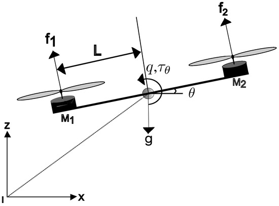
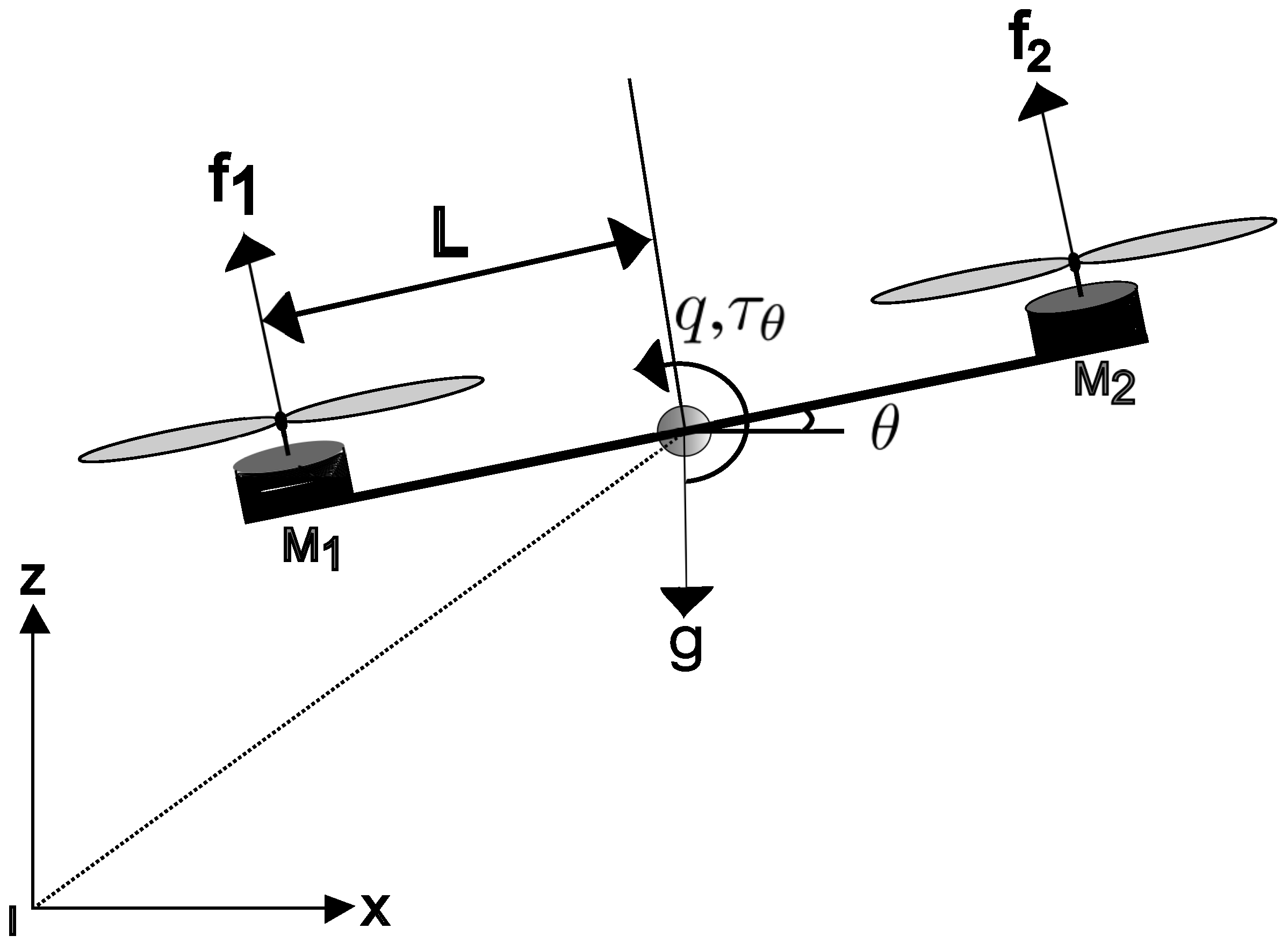
To model the mathematical behavior of the bi-rotor system, it is considered a rigid body in the $x-y$ plane. The external forces acting on the bi-rotor model are the two engines and gravity [26]. Forces are not considered in this model because the bi-rotor system is fixed on a base that does not allow lateral or elevating movement. Therefore, the aerodynamic drag force D, or opposition to lateral movement, and the aerodynamic lift force L, or lift, are ruled out. Figure 1 shows a free-body diagram of the bi-rotor model and the forces acting on the bi-rotor system.

Figure 1. Variables and forces acting on the fixed bi-rotor system.

In this work, the dynamic model describing a vertical take-off unmanned aerial vehicle (VTOL) in the [27,28,29] plane is used. From this model, only the part that defines the dynamics of the angular acceleration at the angle $\theta$ will be utilized. The dynamics of a planar vertical take-off and landing (PVTOL) are then given by the following:

$$\begin{array}{ccc}\hfill \ddot{x}& =& -sin\left(\theta \right)T_t+ϵcos\left(\theta \right)u_{\theta }\hfill \end{array}$$

(1)

$$\begin{array}{ccc}\hfill \ddot{z}& =& cos\left(\theta \right)T_t+ϵcos\left(\theta \right)u_{\theta }-mg\hfill \end{array}$$

(2)

$$\begin{array}{ccc}\hfill \ddot{\theta }& =& u_{\theta }\hfill \end{array}$$

(3)

where x represents the horizontal displacement, z is the vertical displacement, and $\theta$ is the rotation angle. $T_t$ is the total thrust generated by the brushless motors. The parameter $ϵ$ is a coefficient that characterizes or defines a coupling between the motion of the angle $\theta$ and the lateral acceleration, m defines the mass, and g is the gravitational constant. To design the controllers for the bi-rotor system proposed in this work, Equation (3) will be used, but defined as a pure angular rotation:

$$\begin{array}{c}\hfill \dot{\theta }=q\end{array}$$

(4)

$$\begin{array}{c}\hfill \dot{q}={\displaystyle \frac{u_{\theta }}{I_{yy}}}\end{array}$$

(5)

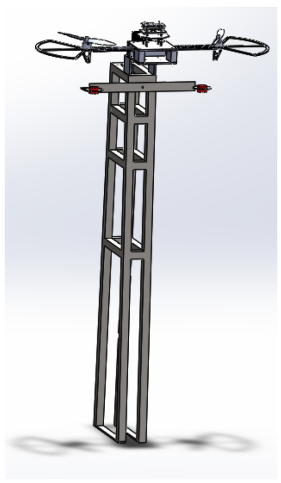
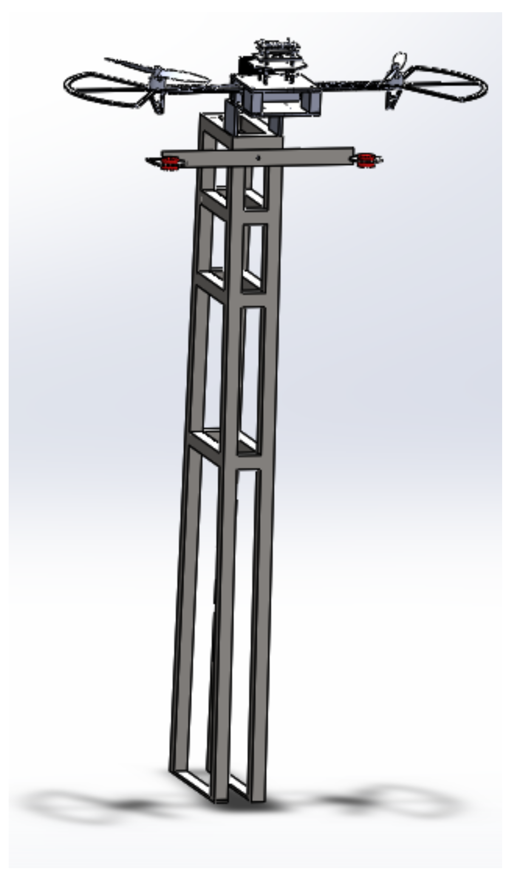
where $q,\theta \in \mathbb{R}$ define the angular velocity and the angle of rotation, respectively. $I_{yy}=0.9946$ is the inertia about the y-axis, calculated from a model developed in SolidWorks (see Figure 2). $u_{\theta }={\tau }_{\theta }$ represents the control input of the bi-rotor system.

Figure 2. Model developed in SolidWorks.

3. Linear and Non Linear Controllers Design

The selection of linear and nonlinear controllers presented in this work is motivated by the observation that, in linear control, the first control laws to study are proportional, derivative, and integral actions, and that the literature contains extensive information on these linear controllers [30,31]. Also, these linear control laws are usually used in the industry, as they are presented in [32,33].

The nonlinear control theory discussed in this work is well known [22,25,34,35]; however, the scientific literature includes numerous computer simulation results. These theories can be experimentally validated using a fixed bi-rotor testbed to provide practical experience for undergraduate or graduate engineering students.

Control laws are defined or composed of proportional, integral, and derivative action [31,32]; the system error is defined by $e_{\theta }=\theta -{\theta }_d$, ${\theta }_d$ is the desired angle, and $\theta$ is the actual angle. Then, the proportional control law (P) is defined as follows:

$$u_{\theta }=k_p{e}_{\theta }$$

(6)

where $k_p$ is a positive definite gain. The proportional derivative (PD) controller to stabilize the bi-rotor system is given by the following:

$$u_{\theta }=k_p{e}_{\theta }+k_d{\dot{e}}_{\theta }$$

(7)

where $k_p$ and $k_d$ are positive definite constants. The proportional integral derivative (PID) controller to stabilize the system defined by (4) and (5) is given by the following:

$$u_{\theta }=k_p{e}_{\theta }+k_i\int e_{\theta }dt+k_d{\dot{e}}_{\theta }$$

(8)

with $k_p,k_d,k_i>0$. For the design of the nonlinear controllers, Equations (4) and (5), which define the dynamic model of the fixed bi-rotor, will be considered. So, for the controller based on the nonlinear control technique known as backstepping [22,34,36], we start by defining a Lyapunov candidate function:

$$V_{1\theta }={\displaystyle \frac{1}{2}}{e}_{\theta }$$

(9)

To continue with the derivation of the backstepping controller, we obtain the derivative of (9), which is $V_{1\theta }=e(q-{\dot{\theta }}_d)$ and define a $z_{\theta }=q-{\dot{\theta }}_d+k_{1\theta }{e}_{\theta }$. After algebraic operations, we have the following:

$${\dot{V}}_{1\theta }=-k_{1\theta }{e}_{\theta }^2+e_{\theta }{z}_{\theta }$$

(10)

Because the derivative (10) is not negative definite, a new candidate Lyapunov function is defined, given by the following:

$$V_{2\theta }=V_{1\theta }+{\displaystyle \frac{1}{2}}{z}_{\theta }^2$$

(11)

Deriving (11), we have the following:

$${\dot{V}}_{2\theta }=-k_{1\theta }{e}_{\theta }^2+z_{\theta }({\displaystyle \frac{u_{\theta }}{I_{yy}}}-{\dot{\theta }}_d+k_{1\theta }{e}_{\theta }+e_{\theta })$$

(12)

So the backstepping control law is defined as follows:

$$u_{\theta }=({\dot{\theta }}_d-k_{1\theta }{e}_{\theta }-e_{\theta }-k_{2\theta }{z}_{\theta })I_{yy}$$

(13)

Then the final derivative of (12) is given by the following:

$${\dot{V}}_{2\theta }=-k_{1\theta }{e}_{\theta }^2-k_{2\theta }{z}_{\theta }^2<0$$

(14)

Thus, with (14) negative definite, it is possible to conclude global asymptotic stability with the backstepping controller defined by Equation (13). For the design of the control law based on nested saturations, a linear transformation $z=T_{zx}x$ of the (4) and (5) [35,37] system will be performed.

$$\begin{array}{ccc}\hfill {\dot{z}}_{1\theta }& =& z_{2\theta }\hfill \end{array}$$

(15)

$$\begin{array}{ccc}\hfill {\dot{z}}_{2\theta }& =& {\displaystyle \frac{u_{\theta }}{I_{yy}}}\hfill \end{array}$$

(16)

So,

$$\begin{array}{ccc}\hfill \left[\begin{array}{c}{z}_{1\theta }\\ z_{2\theta }\end{array}\right]& =& \left[\begin{array}{cc}{k}_{2\theta }{k}_{1\theta }& k_{2\theta }\\ 0& k_{1\theta }\end{array}\right]\left[\begin{array}{c}{x}_{1\theta }\\ x_{2\theta }\end{array}\right]\hfill \end{array}$$

(17)

where $k_{2\theta },k_{1\theta }>0$, $x_{1\theta }=\theta$ and $x_{2\theta }=q$. The saturation function is defined by ${\sigma }_a:\mathbb{R}\to \mathbb{R}$ with limit a:

$${\sigma }_a\left(s\right)=\left\{\begin{array}{cc}\hfill -a,& s<-a\hfill \\ \hfill s,& -a\le s\le b\hfill \\ \hfill a,& s>a\hfill \end{array}\right.$$

(18)

where a is a positive constant value; then, for the (4) and (5) system defined by a linear transformation as in (17) and the saturation function (18), the nested saturation controller to achieve global asymptotic stability is given by the following:

$$u_{\theta }=-{\sigma }_2(z_{2\theta }+{\sigma }_1\left(z_{1\theta }\right))I_{yy}$$

(19)

Finally, the sliding mode controller (SMC) to stabilize the (4) and (5) system defines a sliding surface $s_{\theta }=q+k_{1\theta }(\theta -{\theta }_d)$ [22,23,24,25], and deriving the sliding surface, we have the following:

$${\dot{s}}_{\theta }={\displaystyle \frac{u_{\theta }}{I_{yy}}}+k_{1\theta }(\theta -{\theta }_d)$$

(20)

Thus, the sliding mode controller is defined by the following:

$$u_{\theta }=(-k_{1\theta }(\theta -{\theta }_d)-{\beta }_{\theta }sign\left(s_{\theta }\right))I_{yy}$$

(21)

with $k_{1\theta },{\beta }_{\theta }>0$ as the controller gains, and the sign function is given as follows:

$$sign\left(s_{\theta }\right)=\left\{\begin{array}{cc}\hfill 1,& s_{\theta }>0\hfill \\ \hfill 0,& s_{\theta }=0\hfill \\ \hfill -1,& s_{\theta }<0\hfill \end{array}\right.$$

In Appendix A and Appendix B the stability proof for the linear and nonlinear controllers, respectively, is presented.

4. Fixed Bi-Rotor Testbed

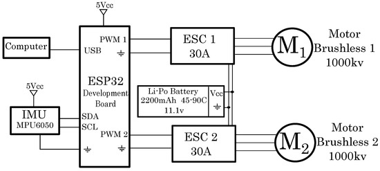
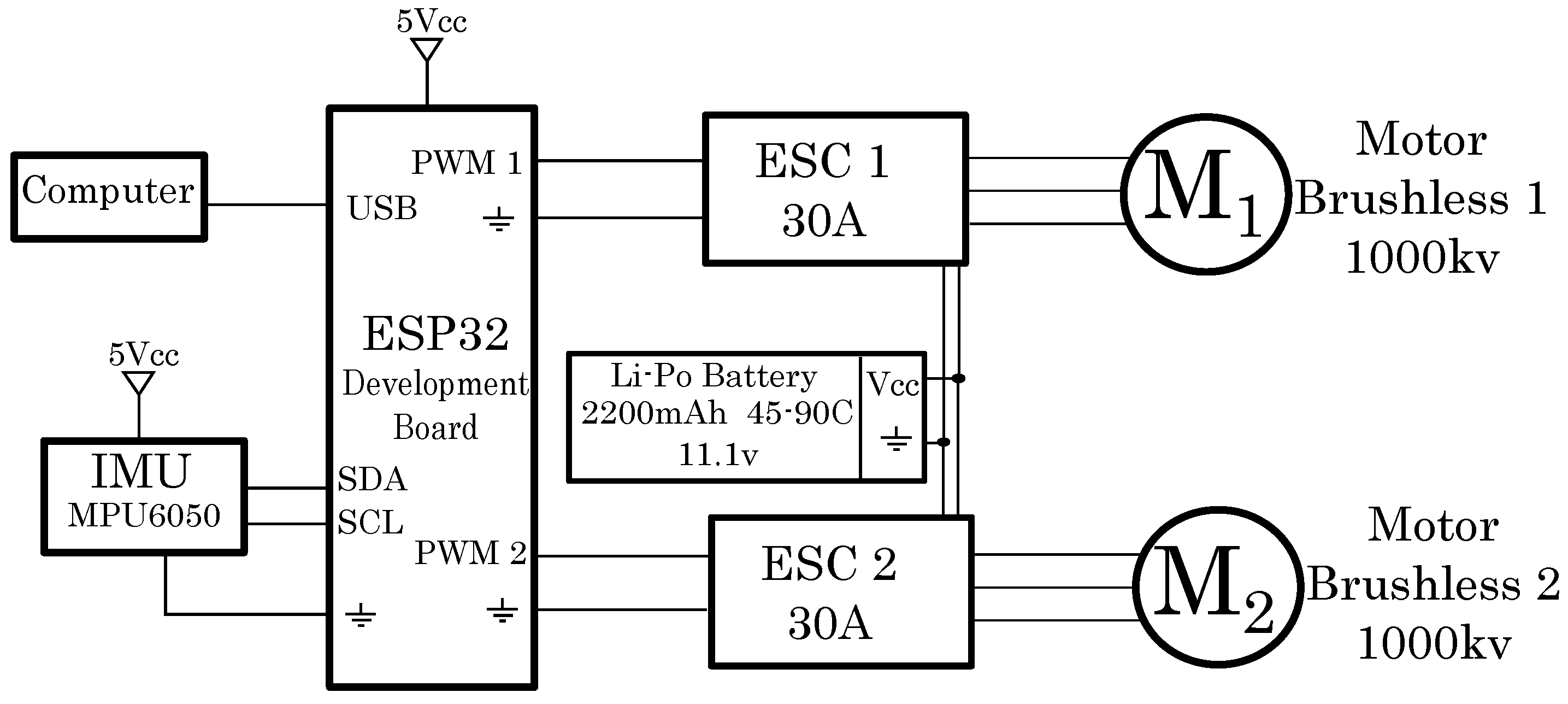
In the fixed bi-rotor testbed, the rotation is produced by adjusting the speeds of the two motors. The motors or actuators are two 1000 KV brushless motors, each paired with a 30 A ESC or driver. The propellers have a 10 × 4.5 pitch. The sensor used to measure the angle and angular rate is an MPU6050.

To program the linear and nonlinear control laws, we used the ESP32 development board [38,39]; the same ESP32 microcontroller is used to read the inertial measurement unit and feed the control laws. The battery powering the entire system is a 2200 mAh Li-Po type battery with discharge cycles of 45–90, and the rotation angle $\theta$ is between $\pm {30}^{\circ }$. The computer connected to the ESP32 loads the linear and nonlinear controller programs, and the same computer is used to adjust the gain values and display the data in real time on the screen.

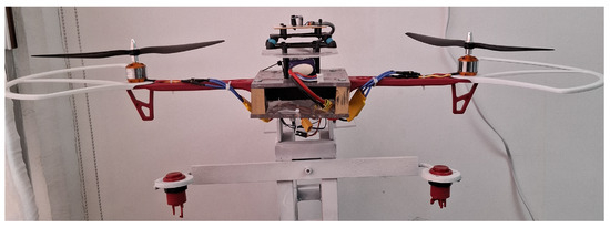
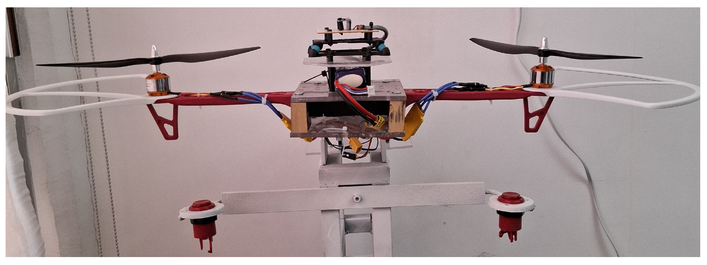
In Figure 3, the general electronic diagram used in the fixed-rotor testbed is shown, and in Figure 4, a picture of the fixed-rotor testbed is displayed.

Figure 3. Electronic diagram used in the fixed bi-rotor testbed.

Figure 4. Fixed bi-rotor testbed.

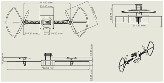
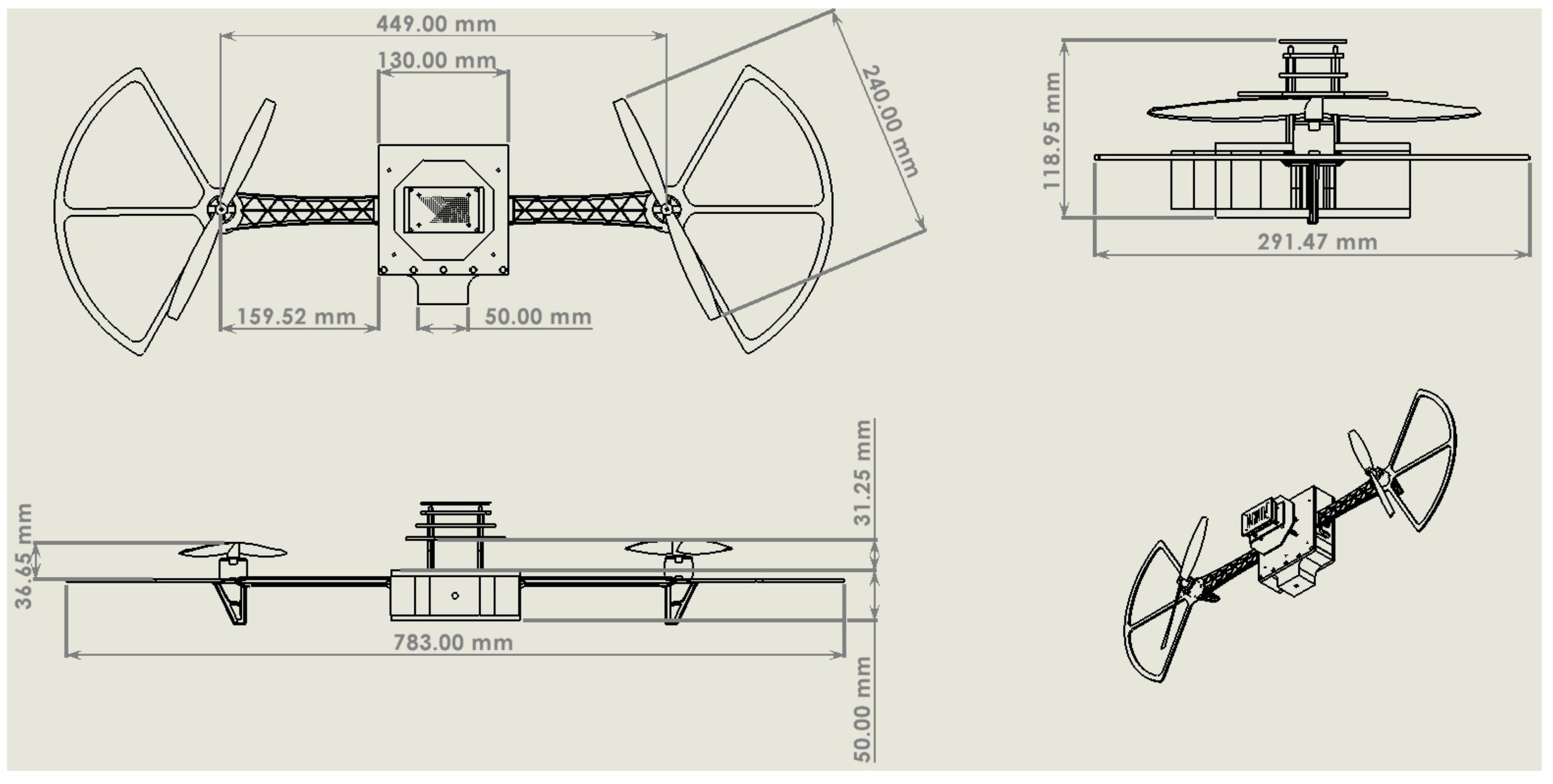
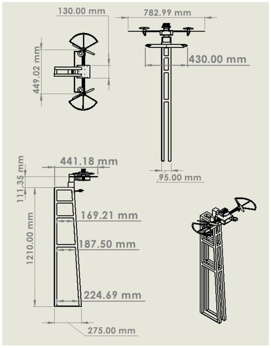
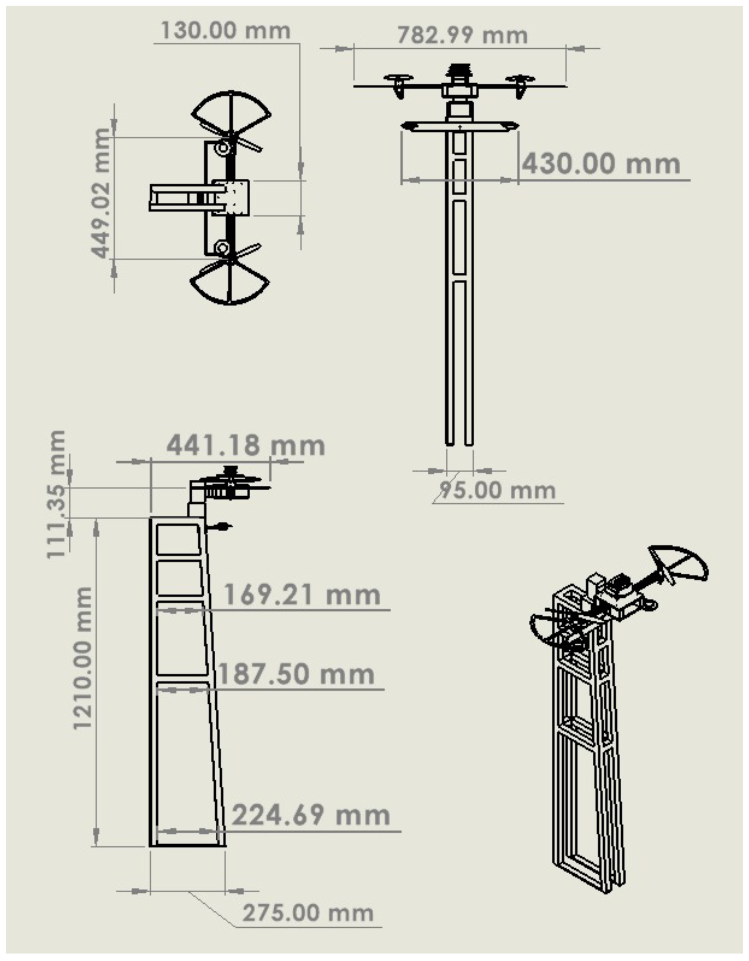
Figure 5 and Figure 6 show the measurements of the rotary frame and the structural measurements in millimeters of the fixed bi-rotor testbed, respectively. Table 1 presents the components used in the fixed bi-rotor testbed.

Figure 5. Measurements of the rotary frame in the fixed bi-rotor in millimeters (mm).

Figure 6. Fixed bi-rotor structural measurement in millimeters (mm).

Table 1. Components used in the fixed bi-rotor testbed.

Component	Model	General Characteristics
IMU	MPU6050	Combines 3-axis acceleration and 3-axis angular rate sensing
Development board	ESP32	Dual-core (or single-core) 32-bit Tensilica Xtensa LX6/LX7 CPU, clockable up to 240 MHz.
Brushless Motor	A2212/13T	1000 rpm/v, 14 poles.
ESC	30 Amp	Input voltage: 2–4 cells Li-Po battery, 5 V, 3 Amp for external receiver and servos.
Battery	lithium polymer Li-Po	2200 mAh 3S (11.1 V) 30C
Propeller	2-blade propeller	Shaft diameter: 6 mm/0.24”; Size: 10 × 4.5”.
Propeller protection	F450/550	10 inch protective ring, quadcopter, hexacopter, drone propeller collision over.
Metal structure	Rectangular Tubular Profile	1” × 1” Gauge 14

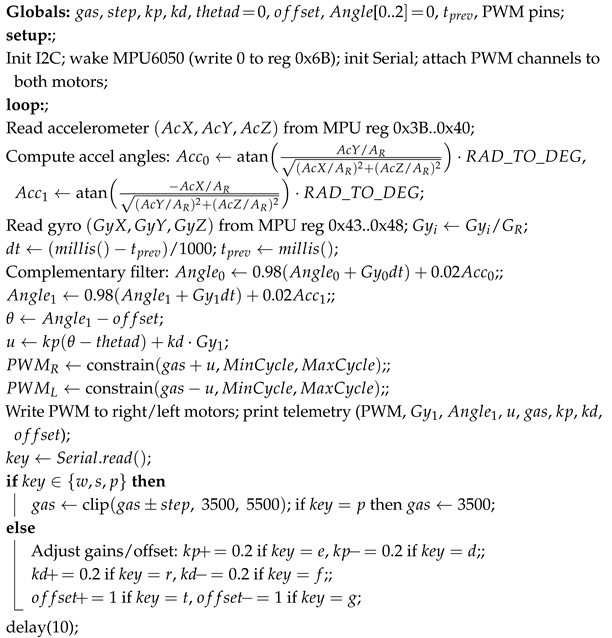
To control the fixed-rotor with a unique control law for two brushless motors, it is necessary to use a differential mode. This involves defining two PWM outputs in the program code: one for brushless motor one and the other for brushless motor two. These program codes include, for one motor, the throttle plus the control law, while the second brushless motor implicitly has in the program code the throttle minus the control law; in this way, it is possible to operate with a single control law for this testbed.

Algorithm 1, the pseudo-code for the PD control law, is presented; the same pseudo-code principles are used to develop the linear and nonlinear controllers.

Algorithm 1: PD Control Law for the fixed bi-rotor tesbed.

5. Experimental Results

The experimental results in this section were collected in an indoor robotic laboratory, free of outdoor wind gusts.

To compare the controllers presented in this work, the ${\mathcal{L}}_2$ norm is used to quantify the error, and the control effort applied to a fixed bi-rotor system is used to quantify the control effort. Thus, the ${\mathcal{L}}_2$- $norm$ norm for the error is defined as follows:

$${\mathcal{L}}_2\left[e_{\theta }\right]=\sqrt{{\displaystyle \frac{1}{T-t_0}}{\int }_{t_0}^T{\parallel e_{\theta }\parallel }^{2}dt}$$

(22)

After, the same norm is applied to calculate the control effort applied by each controller to stabilize the fixed bi-rotor system, and is defined by the following:

$${\mathcal{L}}_2\left[u_{\theta }\right]=\sqrt{{\displaystyle \frac{1}{T-t_0}}{\int }_{t_0}^T{\parallel u_{\theta }\parallel }^{2}dt}$$

(23)

Table 2 presents the results obtained by applying the ${\mathcal{L}}_2$ norm for the analysis of the error and the controller effort applied by the controllers presented in this work. Table 3 presents the gains used in the experimental approaches presented in this work.

Table 2. ${\mathcal{L}}_2$-$norm$ error and control effort in roll angle.

Controller	${\mathcal{L}}_2\left[{\mathit{e}}_{\mathit{\varphi }}\right]$	${\mathcal{L}}_2\left[{\mathit{u}}_{\mathit{\theta }}\right]$
P	4.3011	30.9673
PD	2.7676	25.0884
PID	5.5522	39.3293
Backstepping	3.2589	19.6441
NS	5.3680	147.9024
SMC	4.2606	144.0976

Table 3. Linear and nonlinear controller gains.

Controller	${\mathit{k}}_{\mathit{p}}$	${\mathit{k}}_{\mathit{i}}$	${\mathit{k}}_{\mathit{d}}$	${\mathit{k}}_{1\mathit{\theta }}$	${\mathit{k}}_{2\mathit{\theta }}$	${\mathit{\beta }}_{\mathit{\theta }}$	${\mathit{\sigma }}_1$	${\mathit{\sigma }}_2$
P	−7.2	-	-	-	-	-	-	-
PD	−7.2	-	−2	-	-	-	-	-
PID	−7.2	−3	−2	-	-	-	-	-
Back	-	-	-	1	4.5	-	-	-
NS	-	-	-	14	7	-	±300	±500
SMC	-	-	-	4	-	1.2	-	-

We have obtained the gains through several experimental tests in a heuristic form, considering the stability proofs presented in Appendix A and Appendix B, respectively. This is because, as is known, there is no exact dynamical model that describes a plant or process to control and obtain the gains for the first time in a theoretical form [30]. Such calculated gains in the theory cannot be used in practice to obtain the desired performance at the first tests. In real practice or experiments, it is necessary to tune the gains in the control laws to achieve the desired performance, as is demonstrated [26,28,32,40].

To ensure the control objective, we have presented linear and nonlinear controllers with corresponding stability proofs. It should be noted that we first conduct computational simulations before the experiments. Still, the context or objective of this work is to demonstrate that the fixed bi-rotor testbed is viable for conducting real-time tests of linear and nonlinear control laws; therefore, computer simulations are omitted.

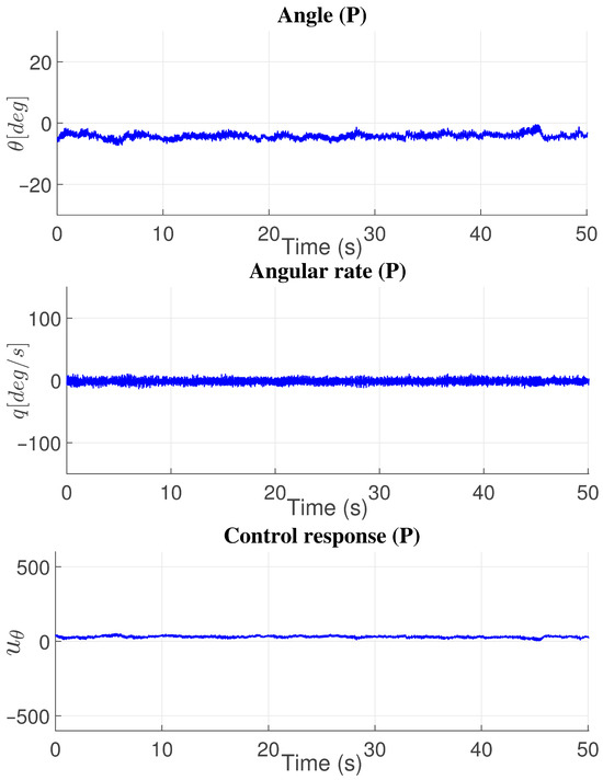
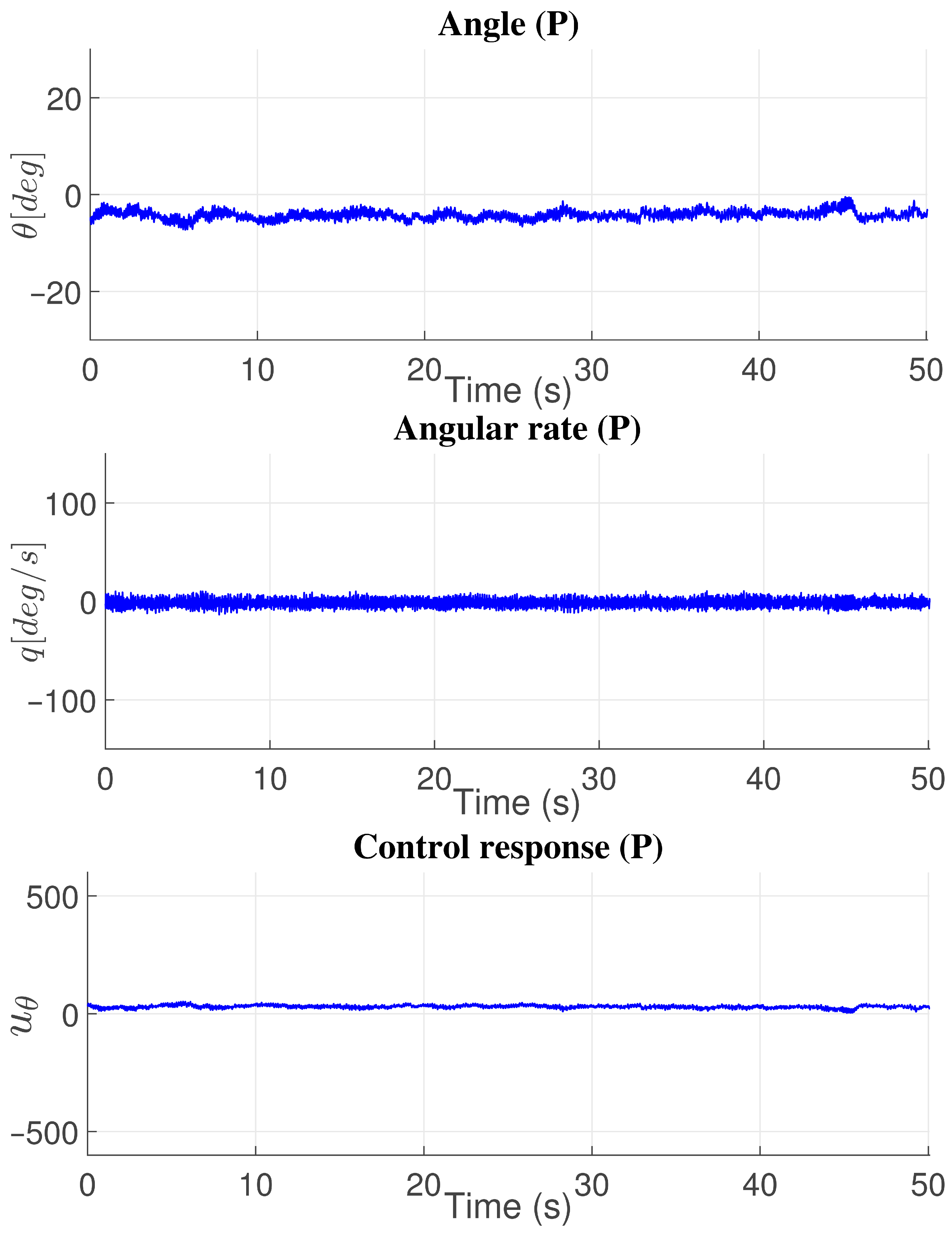
Figure 7 presents the results obtained in experiments applying the proportional controller to the fixed bi-rotor testbed to control the angle $\theta$, with a value of ${\theta }_d=0^{\circ }$. The angle $\theta$ is limited to $\pm {30}^{\circ }$. Figure 7 presents the same data, showing the angular rate and the control signal generated by the proportional controller (P). Compared with the proportional–derivative (PD) and proportional–integral–derivative (PID) controllers, the proportional controller produced bigger errors and control actions. Still, the proportional controller presented a larger error in the angle $\theta$ and control action bigger than the PD controller.

Figure 7. Proportional (P) controller response in $\theta$ angle.

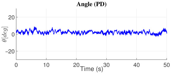
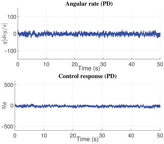
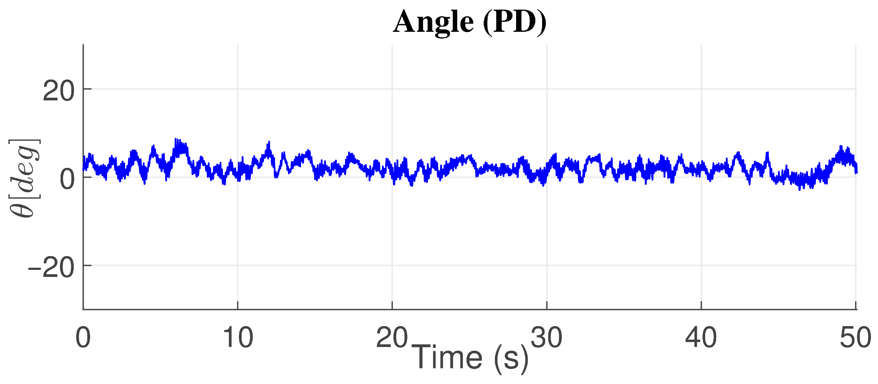
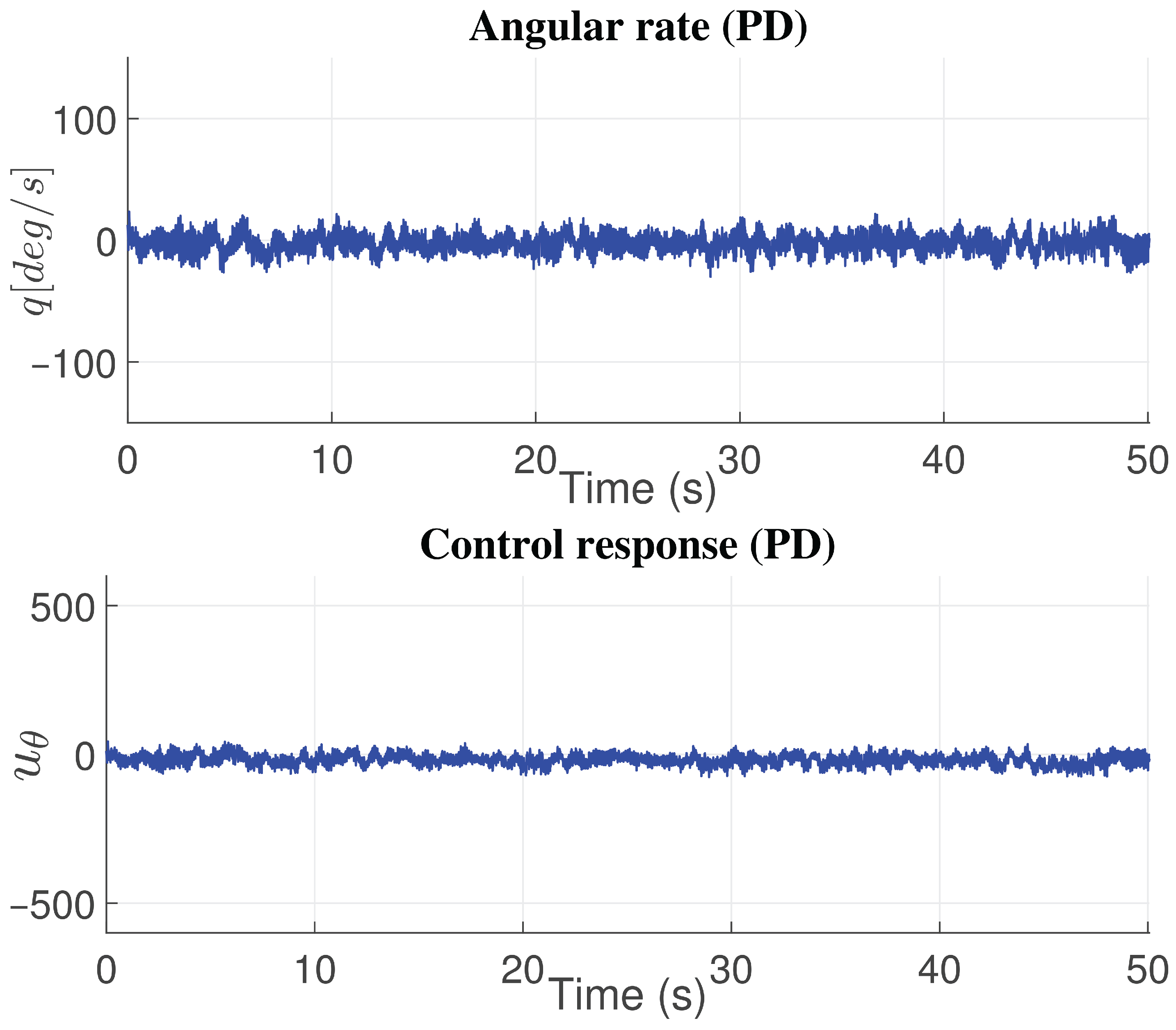
Figure 8 presents the angle response $\theta$, and the angular rate response is obtained by applying the PD control action. The control signal to stabilize the fixed bi-rotor testbed with the PD controller is presented in the same figure (Figure 8). Comparing the PD controller with linear control laws based on proportional and proportional–integral–derivative (PID), the PD controller presented the better responses in terms of error and controller effort compared with the proportional (P) and proportional–integral–derivative (PID) control techniques, as shown in Table 2.

Figure 8. Proportional–derivative (PD) controller response in $\theta$ angle.

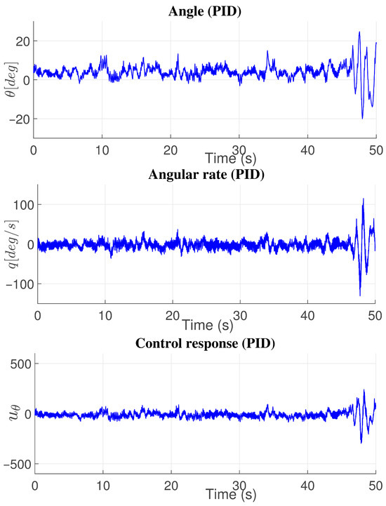
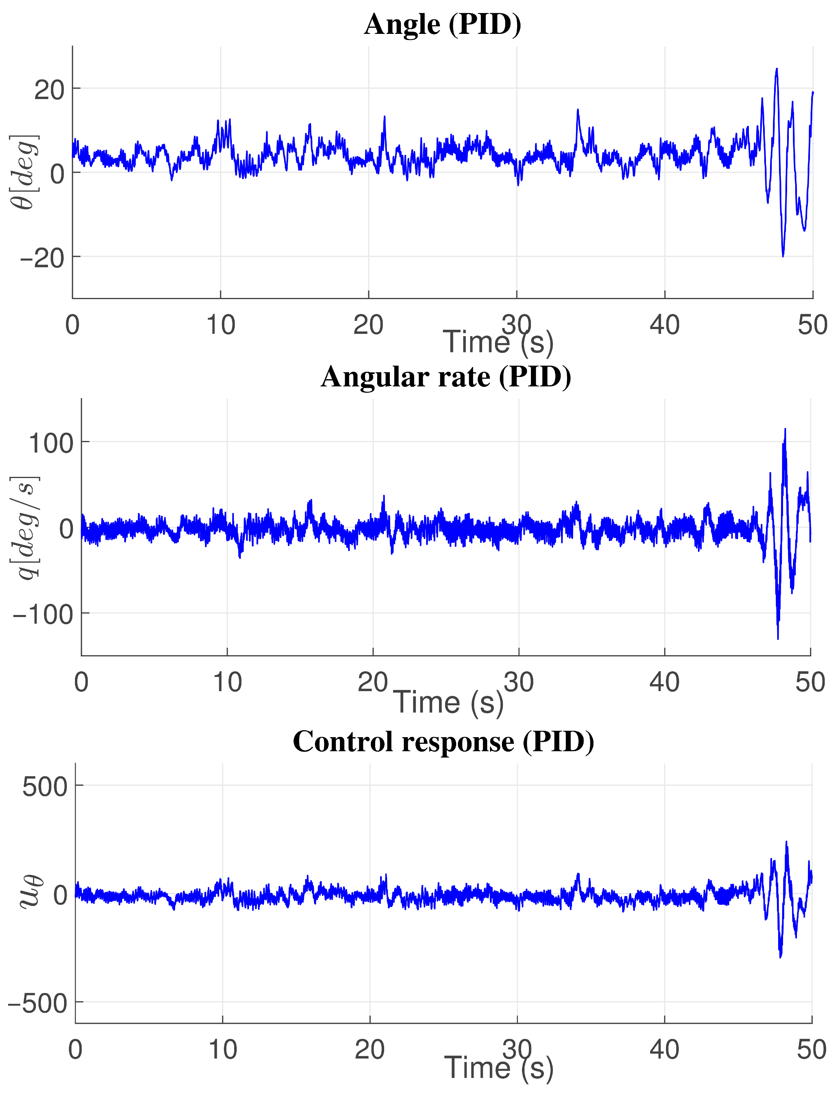
The results obtained in experiments with the PID controller are presented in Figure 9. The exact figure shows the position and angular rate responses of the PID controller. The control signal used to stabilize the bi-rotor testbed via the PID control law is presented in Figure 9. The PID control law exhibited a larger angular error than the linear and nonlinear controllers. It required greater control effort than the linear control laws and the nonlinear backstepping controller (see Table 2).

Figure 9. Proportional–integral–derivative (PID) controller response in $\theta$ angle.

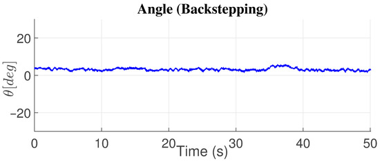
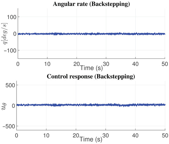
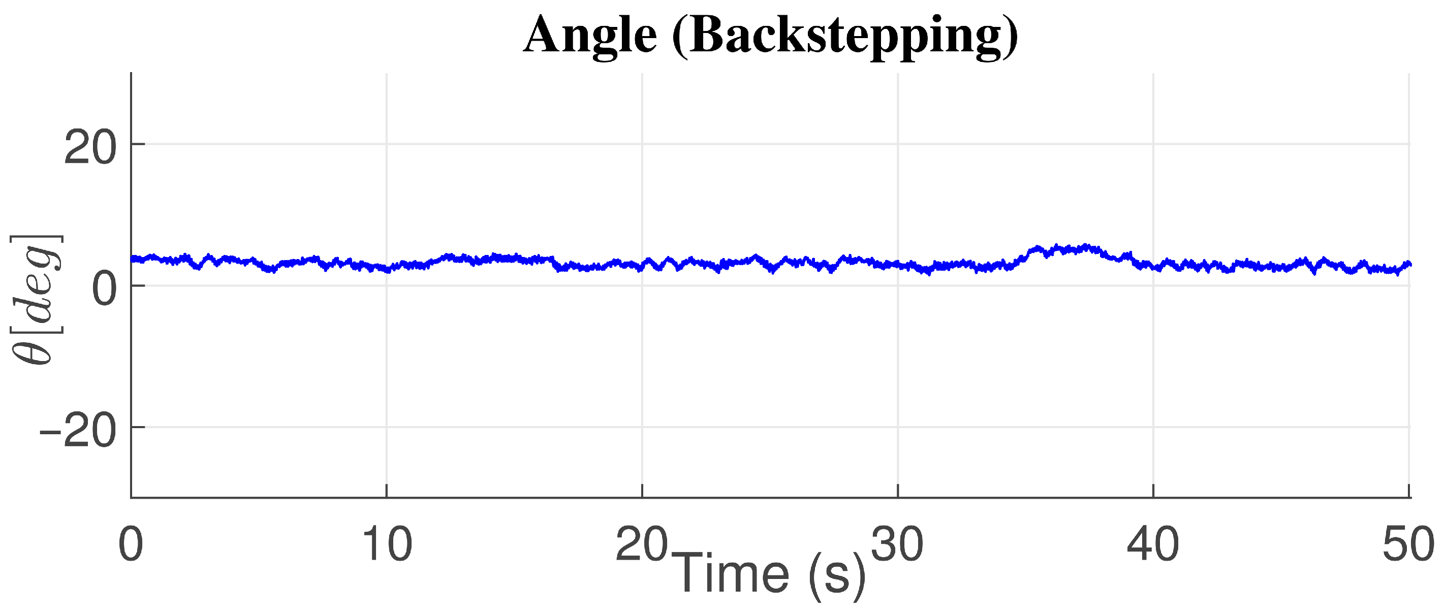
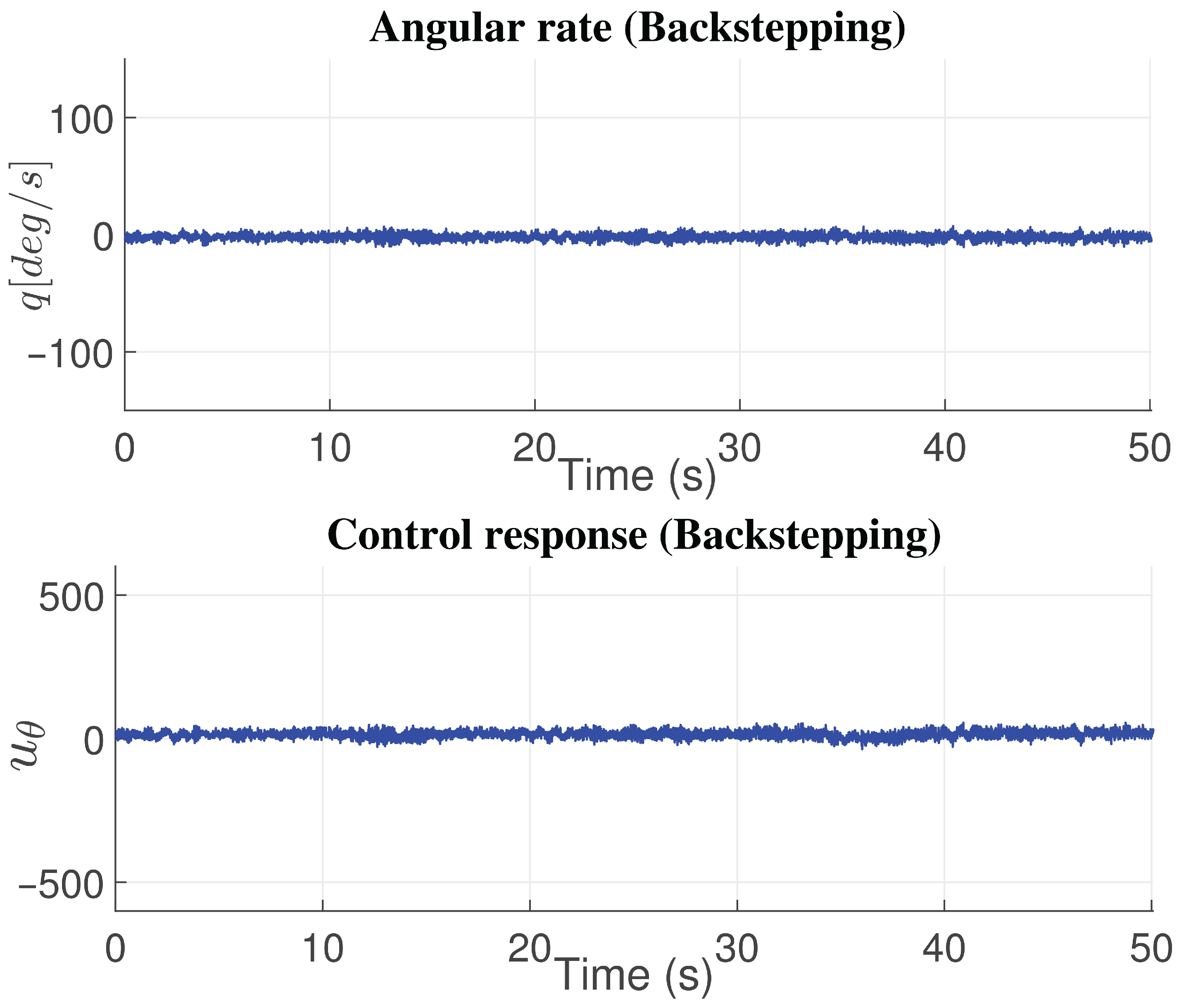
On the other hand, Figure 10 presents the results of the experimental study using the nonlinear backstepping control technique. Figure 10 presents the graphs of angle, angular rate, and controller response. Compared with the linear and nonlinear controllers presented in this work, the backstepping controller presents a smaller control effort to maintain the desired angle ${\theta }_d$ near zero degrees. Still, it is second in error compared to the PD controller, which shows a smaller angular error (see Table 2). Compared with the other nonlinear controllers, nested saturation and SMC, backstepping control presents a better response in both the angular error and the control effort. This is affirmed in Table 2.

Figure 10. Backstepping controller response in $\theta$ angle.

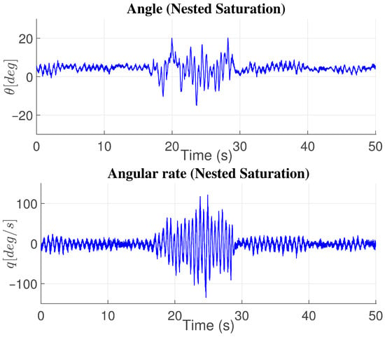
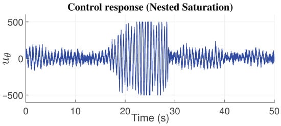
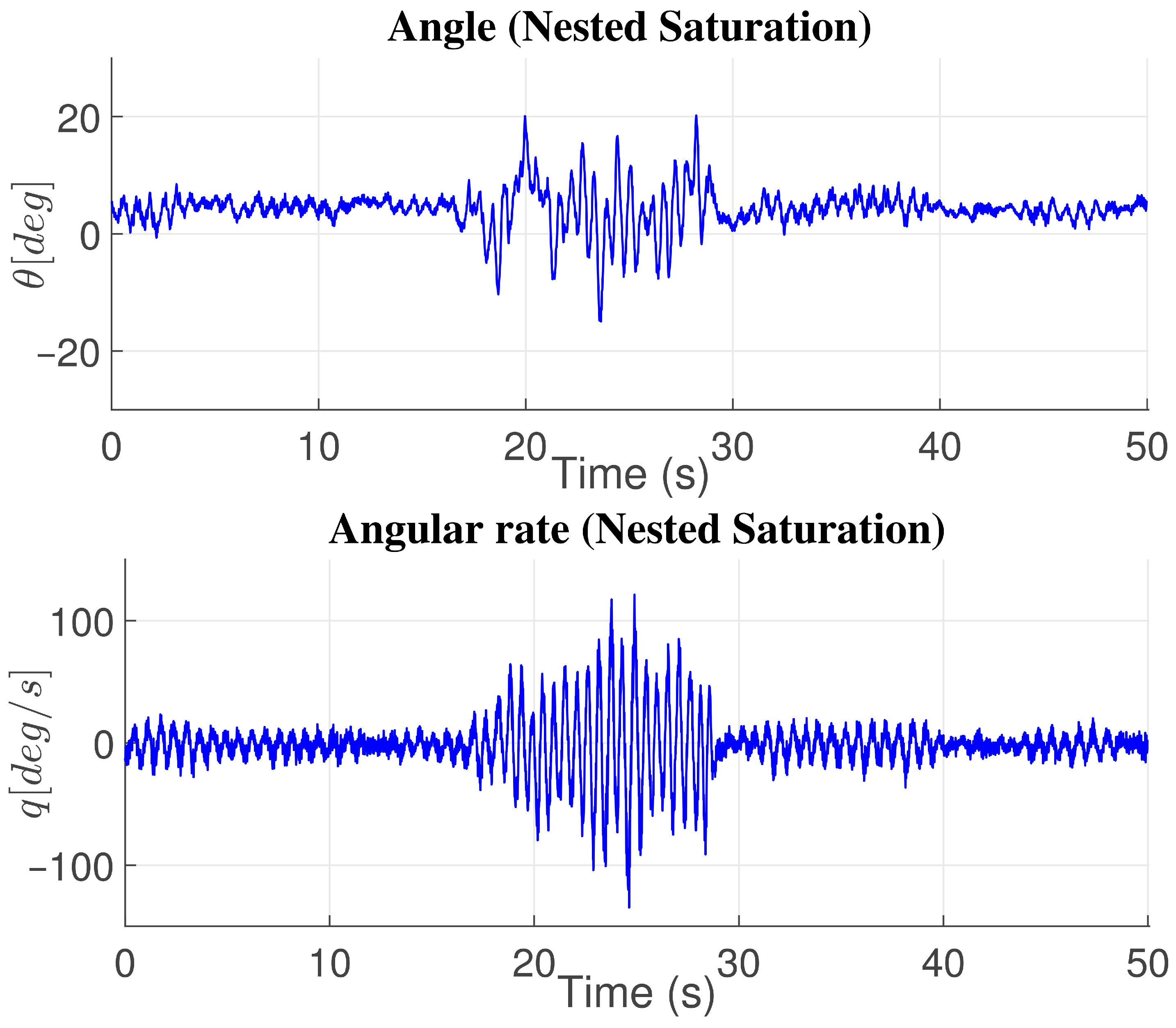
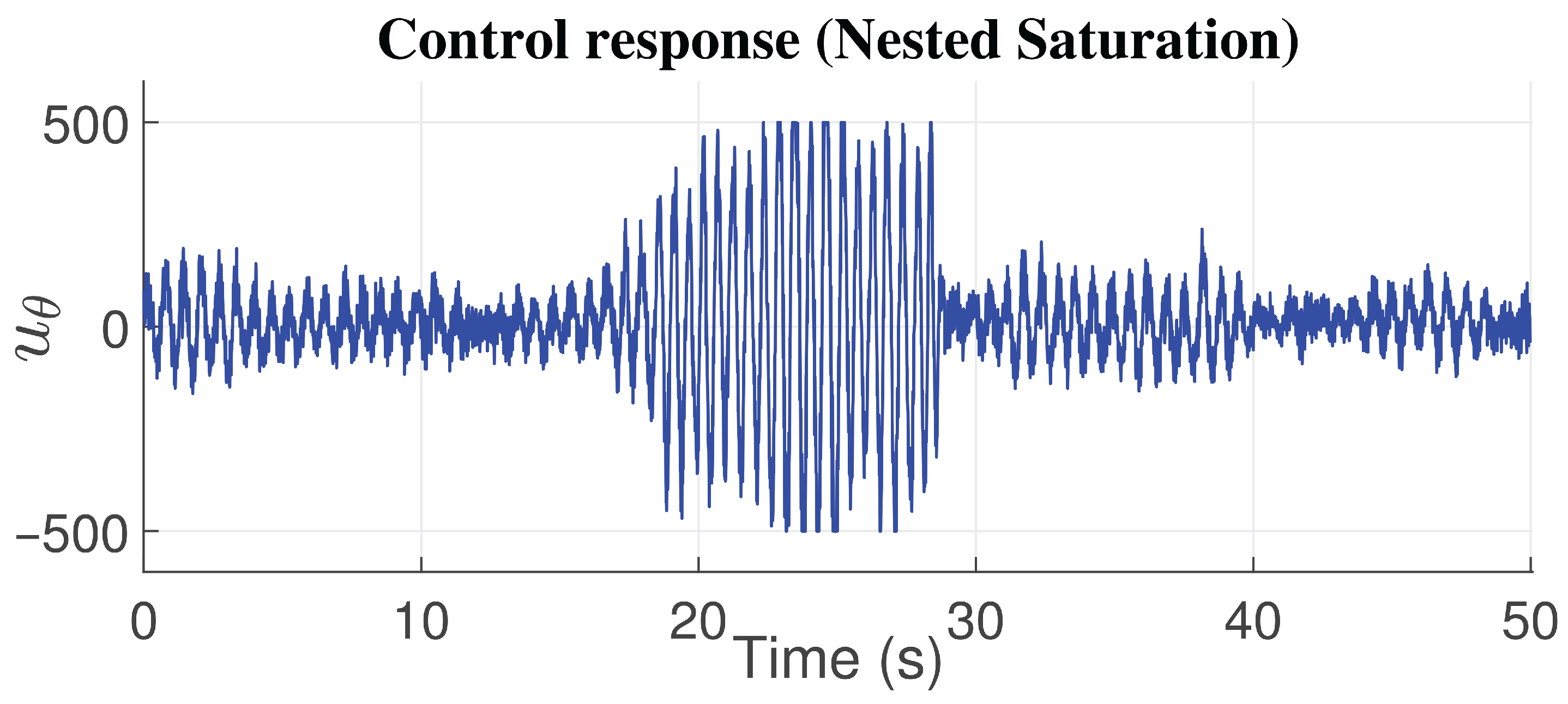
The nested saturation nonlinear controller requires greater control effort than the linear and nonlinear controllers presented in this work. Additionally, the angular error is smaller than that of the PID controller; the PID controller exhibits the most significant angular error (see Table 2). Figure 11 presents the angle, angular rate, and control response graphs with the controller based on nested saturation.

Figure 11. Nested saturation controller response in $\theta$ angle.

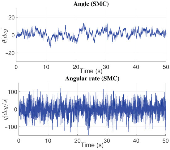
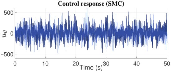
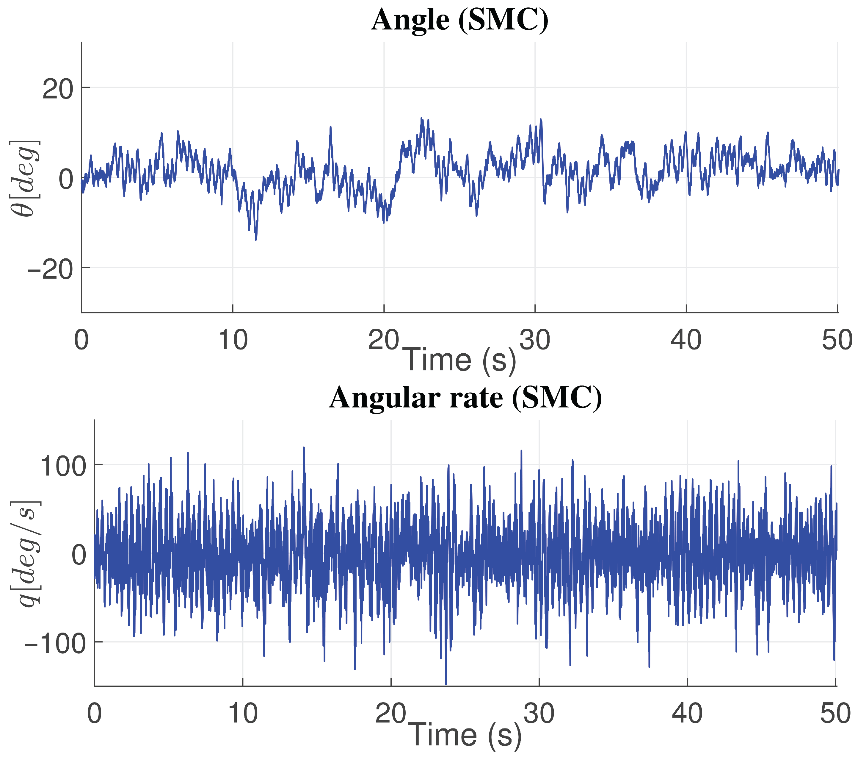
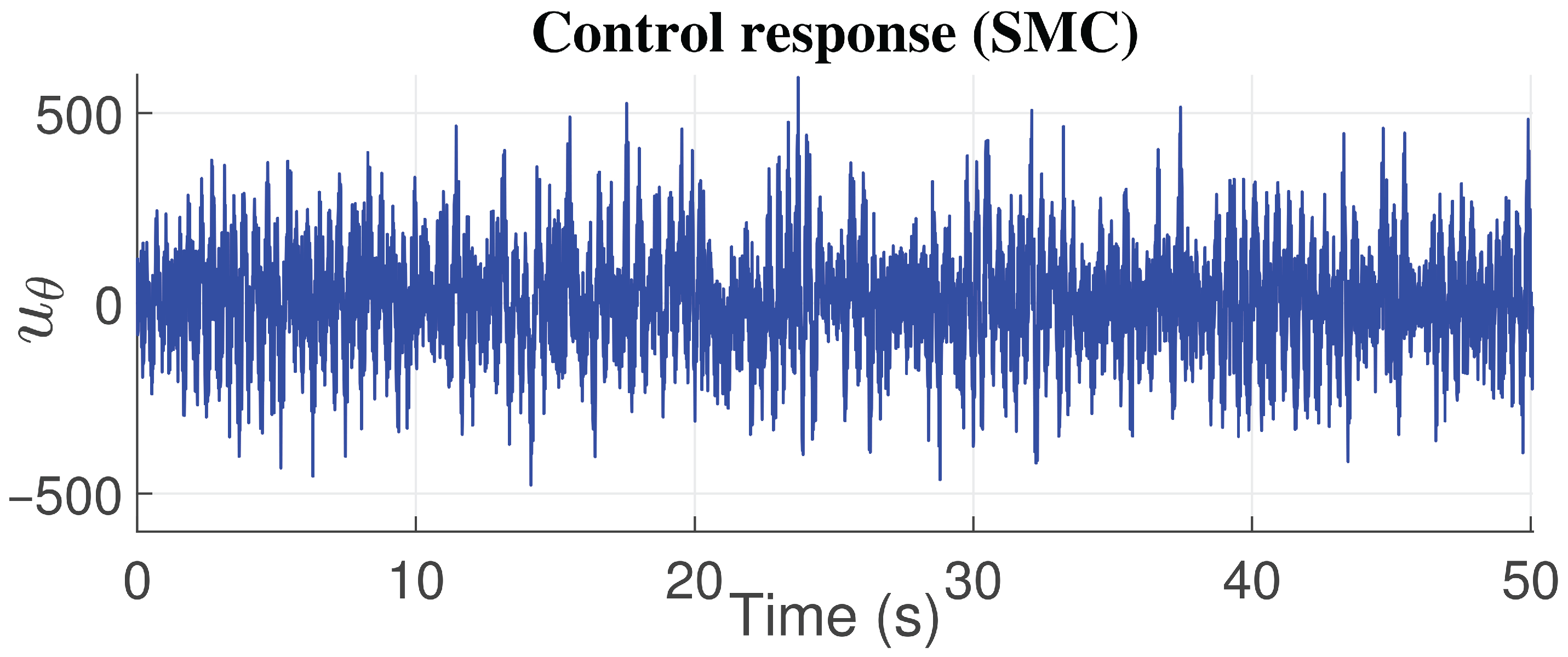
The sliding mode controller (SMC) presented a smaller angular error than the PID controllers and the nested saturation control. In terms of control effort, it is smaller than the nested saturation controller. However, compared with the linear controllers (P, PD, and PID) and backstepping control, the SMC required greater effort to regulate the angle near the desired value of zero degrees along the horizontal axis (see Table 2). Figure 12 presents the graphs of the angle, angular rate, and control response obtained with the nonlinear controller based on first-order sliding modes (SMC).

Figure 12. Sliding mode controller response in $\theta$ angle.

Based on the experimental results presented above, a final table is provided to compare the advantages and disadvantages of each control and and some recommended applications for these control laws (see Table 4).

Table 4. Final comparison of controllers.

Controller	Advantages	Disadvantages	Recommended Applications
P	Low programming cost	Does not achieve the control objective	Recommended for laboratory practice to learn some principles of proportional action, and electronic practice with operational amplifier circuits [30,41].
PD	Middle programming cost	It is necessary to use a development board with sufficient processing speed to compute the derivative error to achieve the control objective.	Drone, serial and parallel robots, robots with wheels [14,28,32,40].
PID	Middle programming cost.	It is necessary to use a development board with sufficient processing speed to compute the derivative and integral actions and achieve the control objective.	Drone, serial and parallel robots [18,21,32,40].
Backstepping	High programming cost	It is necessary to use a development board with sufficient processing speed to process the feedback states in the control law.	Serial robots, remotely operated vehicles, such as quadrotors and fixed-wing UAVs [28,40].
Nested Saturation	High programming cost	It is essential to use a development board with enough processing speed to handle the feedback states and the saturation function in the control law.	Remotely operated vehicles, such as quadrotors and fixed-wing UAVs  [26,28,37,40].
SMC	High programming cost	It is essential to use a development board with enough processing speed to handle the feedback states and the sign function in the control law.	Remotely operated vehicles, such as quadrotors and fixed-wing UAVs [40,42].

6. Discussion

This paper presents a testbed for learning and teaching linear and nonlinear control theory, as well as for other fields such as electronics and programming. To evaluate the feasibility of using the fixed bi-rotor testbed, we collected the best results from several tests with linear and nonlinear controllers: proportional (P), proportional–derivative (PD), and proportional–integral–derivative (PID), backstepping, nested saturation, and sliding modes. The testbed was built using affordable electronic components and steel. This aims to allow other universities and research centers to replicate it and facilitate learning in automatic control theory and related fields. Other platforms or testbeds for teaching control theory and some other topics in electronics and programming are presented in [5]. The differences of fixed bi-rotor testbeds presented in [5] are used for linear control laws for the P, PD, and PID controllers, and, with the fixed bi-rotor testbed, it is possible to address or cover these topics and others that arise [5].

In [43], a building performance simulator applied model-predictive control theory and OpenAI Gym to simulate different environments. The difference between this and the fixed bi-rotor testbed is that we do not have a real-time simulator; however, before the linear and nonlinear control law testbed, we conducted several simulations to assess the testbed’s performance.

On the other hand, in [6], a low-cost, low-risk testbed for launch vehicles is described, but only the prototype’s dynamic model is presented. The difference between [6] and the fixed bi-rotor testbed is that [6] has identified every constant used in the launch vehicle prototype in numerical form.

We can find works with better experimental results than those presented by the fixed bi-rotor testbed, such as [8,11,13,14,15,18,20,40]. It is possible to obtain better responses with the fixed bi-rotor testbed. Still, this implies a more advanced inertial measurement unit, which could increase the platform’s cost, and this does not lend itself to easy replication by students.

We cannot lose sight of the fact that the fixed bi-rotor testbed is designed to be replicated using low-cost, easily accessible components for teachers, students, universities, and laboratories that lack significant financial backing to develop platforms that support their learning and training as engineers or scientists.

It is clear that the fixed bi-rotor testbed has physical and electronic limitations as it presents only a unique degree of freedom by the angle $\theta$, which is limited to $\pm {30}^{\circ }$; furthermore, the brushless motors are limited to work at 80% of velocity as maximum to avoid damage in the motors, and the sensor presents high noise. However, we consider that professors and students can use these limitations to conduct studies in electronics, programming, control theory, and filtering analysis, among others.

7. Conclusions

Comparing the three linear controllers, it was concluded that the PD controller provided the best control response. This is because when the errors of the controllers and the control efforts to achieve the control objective were analyzed using the ${\mathcal{L}}_2$ norm, the PD controller showed smaller error and smaller control effort in comparison with the linear proportional (P) and proportional–integral–derivative (PID) controllers.

Among nonlinear controllers, the backstepping controller yielded the better response in terms of angular error and control effort. The nested saturation control showed larger angular error and control effort than the nonlinear controllers. The sliding-mode controller achieved the control objective, albeit with well-known chattering in the control signal, and required greater control effort than the backstepping controller and the three linear control laws.

Thus, in a comparison of linear and nonlinear controllers, the nonlinear controller based on the backstepping technique demonstrated better performance.

In the following list, we present the future work perspectives derived from the fixed bi-rotor testbed:

• Develop a signal-filtering implementation to improve the MPU6050 inertial measurement unit’s response.
• We will use an additional low-cost development board with greater processing capabilities for computing more advanced control algorithms.
• To test other linear and nonlinear control laws, such as adaptive control, model reference adaptive control MRAC self-tuning regulator STR, linear quadratic regulator (LQR), and linear quadratic Gaussian (LQG), to carry out more practices in the robotic or control laboratory for the students.
• Carrying out a deep theory analysis considering the sensor noise, unmodeled parameters, system vibrations, and parameter sensitivity, considering the works of [44,45,46,47,48,49], to obtain better responses with the fixed bi-rotor testbed.

Finally, we have added a link to the tests in video form (https://youtu.be/jFUBUMt5jQ4, accessed on 23 November 2025).

Appendix C.1. Backstepping

Consider the following result [22]:

Theorem A5.

Let $x_{\theta }=0$ be a uniformly asymptotically stable equilibrium point of the nominal system $x_{\theta }=f\left(x_{\theta }\right)$. Let $V(t,x_{\theta })$ be a Lyapunov function of the nominal system that satisfies the inequalities

$$\begin{array}{c}\hfill {\alpha }_1(\parallel x_{\theta }\parallel )\le V(t,x_{\theta })\le {\alpha }_2(\parallel x_{\theta }\parallel ),\end{array}$$

(A33)

$$\begin{array}{c}\hfill {\displaystyle \frac{\partial V}{\partial t}}+{\displaystyle \frac{\partial V}{\partial x_{\theta }}}f\left(x_{\theta }\right)\le -{\alpha }_3(\parallel x_{\theta }\parallel ),\end{array}$$

(A34)

$$\begin{array}{c}\hfill ∥{\displaystyle \frac{\partial V}{\partial x_{\theta }}}∥\le {\alpha }_4(\parallel x_{\theta }\parallel ),\end{array}$$

(A35)

in $[0,\infty )\times D$, where $D=\left\{x_{\theta }\in {\mathrm{I}\mathrm{R}}^2|\parallel x_{\theta }\parallel <r\right\}$ and ${\alpha }_i(·)$, $i=1,2,3,4$ are class $\mathcal{K}$ functions. Suppose the perturbation term $g(x_{\theta },t)$ satisfies the uniform bound

$$\begin{array}{c}\hfill \parallel g(x_{\theta },t)\parallel \le \delta <{\displaystyle \frac{k{\alpha }_3\left({\alpha }_2^{-1}\left({\alpha }_1\left(r\right)\right)\right)}{{\alpha }_4\left(r\right)}},\end{array}$$

(A36)

for all $t\ge 0$, all $x_{\theta }\in D$ and some positive constant $k<1$. Then for all $\parallel x_{\theta }\left(t_0\right)\parallel <{\alpha }_2^{-1}\left({\alpha }_1\left(r\right)\right)$, the solution of the perturbed system (A30) satisfies

$$\begin{array}{c}\hfill \parallel x_{\theta }\left(t\right)\parallel \le \beta (\parallel x_{\theta }\left(t_0\right)\parallel ,t-t_0),\forall t_0\le t<t_0+T,\end{array}$$

(A37)

and

$$\begin{array}{c}\hfill \parallel x_{\theta }\left(t\right)\parallel \le \rho \left(\delta \right),\forall t\ge t_0+T,\end{array}$$

(A38)

for some class $\mathcal{KL}$ function β and some finite T, where ρ is a class $\mathcal{K}$ function of $delta$ defined by

$$\begin{array}{c}\hfill \rho \left(\delta \right)={\alpha }_1^{-1}\left({\alpha }_2\left({\alpha }_3^{-1}\left({\displaystyle \frac{\delta {\alpha }_4\left(r\right)}{k}}\right)\right)\right)\end{array}$$

(A39)

For the bi-rotor in closed loop with the backstepping controller (13)

$$\begin{array}{cc}\hfill {\alpha }_1(\parallel x_{\theta }\parallel )& ={\displaystyle \frac{1}{2}}{\parallel x_{\theta }\parallel }^2,\hfill \end{array}$$

(A40)

$$\begin{array}{cc}\hfill {\alpha }_2(\parallel x_{\theta }\parallel )& ={\displaystyle \frac{1}{2}}{\parallel x_{\theta }\parallel }^2,\hfill \end{array}$$

(A41)

$$\begin{array}{cc}\hfill {\alpha }_3(\parallel x_{\theta }\parallel )& =-min\left(\{k_{1\theta },k_{2\theta }\}\right){\parallel x_{\theta }\parallel }^2,\hfill \end{array}$$

(A42)

$$\begin{array}{cc}\hfill {\alpha }_3(\parallel x_{\theta }\parallel )& =\parallel x_{\theta }\parallel ,\hfill \end{array}$$

(A43)

So that for $\parallel x_{\theta }\parallel <r$ and if $\delta$ satisfies

$$\begin{array}{c}\hfill \delta <kmin\left(\{k_{1\theta },k_{2\theta }\}\right)r\end{array}$$

(A44)

The solutions $x_{\theta }\left(t\right)$ remain bounded and after some time T the solution will be bounded by

$$\begin{array}{c}\hfill \rho \left(\delta \right)={\displaystyle \frac{\delta r}{kmin\left(\{k_{1\theta },k_{2\theta }\}\right)}}.\end{array}$$

(A45)

Appendix C.2. Nested Saturations

Lets begin finding the closed-loop dynamics of the bi-rotor system subject to disturbances with the control law (19), which is given by

$$\begin{array}{cc}\hfill {\dot{z}}_{1\theta }& =z_{2\theta },\hfill \end{array}$$

(A46)

$$\begin{array}{cc}\hfill {\dot{z}}_{2\theta }& =-{\sigma }_2(z_{2\theta }+{\sigma }_1\left(z_{1\theta }\right))+g(x_{\theta },t).\hfill \end{array}$$

(A47)

For values of q such that $|z_{2\theta }|<{\displaystyle \frac{1}{2}}{L}_2+\delta$

$$\begin{array}{c}\hfill {\dot{z}}_{2\theta }=-(z_{2\theta }-{\sigma }_1\left(z_{1\theta }\right))+g(x_{\theta },t)\end{array}$$

(A48)

Now, consider the Lyapunov function $V_2=z_{1\theta }^2$. The time derivative of this function is

$$\begin{array}{cc}\hfill {\dot{V}}_2& =-z_{2\theta }^2-z_{2\theta }{\sigma }_1\left(z_{1\theta }\right)+g(x_{\theta },t),\hfill \end{array}$$

(A49)

which is negative for values of $z_{2\theta }\notin Q_2=\{z_{2\theta }|{\displaystyle \frac{1}{2}}{L}_2+\delta \}$. This imposes that $\delta <{\displaystyle \frac{1}{2}}{L}_2$, for there to be some values of $z_{2\theta }$ such that the saturation in $\sigma$ is not reached and to ensure that the proof in [35] remains valid.

Appendix C.3. Sliding Modes

The time derivative of the Lyapunov function (A22) along the solutions of the disturbed system (A30) in closed loop with (21) is

$$\begin{array}{c}\hfill \dot{V}=-\beta s_{\theta }sign\left(s_{\theta }\right)+g(x_{\theta },t)s_{\theta }.\end{array}$$

(A50)

This derivative is negative definite if $\delta <{\beta }_{\theta }$, meaning that for disturbances smaller than ${\beta }_{theta}$ the trajectories keep reaching the manifold $s_{\theta }=0$.

References

- Chevallereau, C.; Abba, G.; Aoustin, Y.; Plestan, F.; Westervelt, E.R.; Canudas-De-Wit, C.; Grizzle, J.W. Rabbit: A testbed for advanced control theory. IEEE Control Syst. Mag. 2003, 23, 57–79. [Google Scholar]
- Nagabhushan, V.; Fitz-Coy, N. Scalable, hil, unconstrained 3-axis test bed for attitude control systems. In Proceedings of the AIAA/AAS Astrodynamics Specialist Conference, Toronto, ON, Canada, 2–5 August 2010; pp. 1–13. [Google Scholar]
- Dong, W.; Gu1, G.; Zhu, X.; Ding, H. Development of a quadrotor test bed-modelling, parameter identification, controller design and trajectory generation. Int. J. Adv. Robot. Syst. 2014, 12, 7. [Google Scholar] [CrossRef] [Scilit]
- Valera, A.; Soriano, A.; Vallés, M. Plataformas de bajo coste para la realización de trabajos prácticos de mecatrónica y robótica. Rev. Iberoam. Autom. Inform. Ind. 2014, 11, 363–376. [Google Scholar] [CrossRef] [Scilit]
- Ramírez, E.; Bono, A.; Montijano, E. Una década de experiencias ense ñando electrónica y control con un levitador magnético. Rev. Iberoam. Autom. Inform. Ind. 2024, 21, 318–327. [Google Scholar] [CrossRef] [Scilit]
- Elke, W.J.; Pei, J.; Caverly, R.J.; Gebre-Egziabher, D. A low-cost and low-risk testbed for control design of launch vehicles and landing systems. In Proceedings of the 2021 IEEE Aerospace Conference, Big Sky, MT, USA, 6–13 March 2021; pp. 1–12. [Google Scholar] [CrossRef] [Scilit]
- Hau-Shiue, J.; Kai-Yew, L. Design and control of a two-wheel self-balancing robot using the arduino microcontroller board. In Proceedings of the 2013 10th IEEE International Conference on Control and Automation (ICCA), Hangzhou, China, 12–14 June 2013; pp. 634–639. [Google Scholar] [CrossRef] [Scilit]
- Unluturk, A.; Aydogdu, O. Machine Learning Based Self-Balancing and Motion Control of the Underactuated Mobile Inverted Pendulum With Variable Load. IEEE Access 2022, 10, 104706–104718. [Google Scholar] [CrossRef] [Scilit]
- Muñoz-Hernandez, G.A.; Díaz-Téllez, J.; Estevez-Carreon, J.; García-Ramírez, R.S. ADRC Attitude Controller Based on ROS for a Two-Wheeled Self-Balancing Mobile Robot. IEEE Access 2023, 11, 94636–94646. [Google Scholar] [CrossRef] [Scilit]
- Munyu, K.; Jongwoo, P.; Dong-Il, P.; Chanhun, P.; Joono, C. Dynamic Inversion-Based Real-Time Trajectory Planning Method for Wheeled Inverted Pendulum Using Asymptotic Expansion Technique. IEEE Access 2023, 11, 94805–94821. [Google Scholar] [CrossRef] [Scilit]
- Yongkuk, K.; Sangjoo, K. Balancing-Prioritized Anti-Slip Control of a Two-Wheeled Inverted Pendulum Robot Vehicle on Low-Frictional Surfaces with an Acceleration Slip Indicator. Machines 2023, 11, 553. [Google Scholar] [CrossRef] [Scilit]
- Ji-Hyun, P.; Baek-Kyu, C. Development of a self-balancing robot with a control moment gyroscope. Int. J. Adv. Robot. Syst. 2018, 2018, 1–11. [Google Scholar] [CrossRef] [Scilit]
- Chen, J.; He, N.; Xu, Z.; Dou, M.; He, L. Design and Implementation of a Novel Two-Wheeled Composite Self-Balancing Robot for Stationary Operations in Unknown Terrain. IEEE Access 2025, 13, 86032–86045. [Google Scholar] [CrossRef] [Scilit]
- Saenz, A.; Santibañe, V.; Bugarin, E.; Dzul, A.; Rios, H.; Villalobos-Chin, J. Velocity Control of an Omnidirectional Wheeled Mobile Robot Using Computed Voltage Control with Visual Feedback: Experimental Results. Int. J. Control Autom. Syst. 2021, 19, 1089–1102. [Google Scholar] [CrossRef] [Scilit]
- López, S.; Llama, M.A. Two-Layer Neuro-Adaptive Compensation Control Applied to a 4-Wheeled Omnidirectional Mobile Robo. IEEE Lat. Am. Trans. 2025, 23, 1318–1324. [Google Scholar] [CrossRef] [Scilit]
- Chi-Yi, T.; Kai-Tai, S. Visual Tracking Control of a Wheeled Mobile Robot With System Model and Velocity Quantization Robustness. IEEE Trans. Control Syst. Technol. 2021, 17, 520–527. [Google Scholar] [CrossRef] [Scilit]
- Meza, J.; Santibáñez, V.; Campa, R. An estimate of the domain of attraction for the PID regulator of manipulators. Int. J. Robot. Autom. 2007, 22, 187–195. [Google Scholar] [CrossRef] [Scilit]
- Sifuentes-Mijares, J.; Santibáñez, V.; Meza-Medina, J.L. Nonlinear PID global regulators with selftuned PD gains for robot manipulators: Theory and experimentation. J. Braz. Soc. Mech. Sci. Eng. 2021, 443, 223. [Google Scholar] [CrossRef] [Scilit]
- De León, V.; Pámanes, A.; Santibáñez, V. Evaluación experimental del caminado en tiempo real de un robot bípedo de 5 gdl con marcha basada en movimientos cicloidales. Univ. Politècnica València 2015, 12, 408–418. [Google Scholar] [CrossRef] [Scilit]
- Soto, I.; Campa, R.; Sánchez-Mazuca, S. Modelado y control con compensación de fricción de un sistema pendubot. Rev. Iberoam. Autom. Inform. Ind. 2020, 18, 39–47. [Google Scholar] [CrossRef] [Scilit]
- Hernández-Guzmán, V.; Silva-Ortigoza, R.; Orrante-Sakanassi, J. Automatic Control with Experiments; Springer: London, UK, 2024. [Google Scholar] [CrossRef] [Scilit]
- Khalil, H. Nonlinear Systems; Pearson Education: New York, NY, USA, 2001. [Google Scholar]
- Slotine, J.; Li, W. Applied Nonlinear Control; Pearson: London, UK, 1991. [Google Scholar]
- Shtessel, Y.; Edwards, C.; Fridman, L.; Levant, A. Sliding Mode Control and Observation; Birkhäuser: New York, NY, USA, 2014. [Google Scholar] [CrossRef] [Scilit]
- Utkin, V.; Poznyak, A.; Orlov, Y.; Polyakov, A. Road Map for Sliding Mode Control Design; Springer: Cham, Switzerland, 2020. [Google Scholar] [CrossRef] [Scilit]
- Lozano, R.; Castillo, P.; Dzul, A. Global stabilization of the pvtol realtime application to a mini-aircraft. In Proceedings of the IFAC System, Structure and Control, Oaxaca, Mexico, 8–10 December 2004; pp. 235–240. [Google Scholar]
- Hauser, J.; Sastry, S.; Meyer, G. Nonlinear control design for slightly non-minimum phase systems: Application to V/STOL aircraft. Automatica 1992, 28, 665–679. [Google Scholar] [CrossRef] [Scilit]
- Castillo, P.; Lozano, R.; Dzul, A. Modelling and Control of Mini-Flying Machines; Springer: London, UK, 2005. [Google Scholar]
- Escobar, J.; Lozano, R.; Bonilla, M. Pvtol exact linearization control. Int. J. Control 2019, 94, 1794–1803. [Google Scholar] [CrossRef] [Scilit]
- Ogata, K. Modern Control Engineering; Prentice Hall: Hoboken, NJ, USA, 2009. [Google Scholar]
- Dorf, R.; Bishop, R. Modern Control Systems; Pearson: London, UK, 2016. [Google Scholar]
- Kelly, R.; Santibañez, V.; Loría, L. Control of Robot Manipulators in Joint Space; Springer: New York, NY, USA, 2005. [Google Scholar]
- Rojas, J.; Arrieta, O.; Villanova, R. Industrial PID Controller Tuning: With a Multiobjective Framework Using MATLAB; Springer: London, UK, 2021. [Google Scholar]
- Krstić, M.; Kanellakopoulos, I.; Kokotovic, P. Nonlinear and Adaptive Control Design; Jhon Wiley: New York, NY, USA, 1995. [Google Scholar]
- Teel, A. Global stabilization and restricted tracking for multiple integrators with bounded controls. Syst. Control Lett. 1992, 18, 165–171. [Google Scholar] [CrossRef] [Scilit]
- Vaidyanathan, S.; Taher, A. Backstepping Control of Nonlinear Dynamical Systems (Advances in Nonlinear Dynamical Systems and Robotics; Academic Press: London, UK, 2020. [Google Scholar]
- Lozano, R.; Salazar, S.; Flores, D.; Gonzalez, I. PVTOL global stabilisation using a nested saturation control. Int. J. Control 2022, 95, 2656–2666. [Google Scholar] [CrossRef] [Scilit]
- Punguil, A.; Rojas, J.; Guillen, M.; Herrerra, E. Introduction Manual for the Use and Applications of the ESP32 Card. Rev. Cient. Generando 2024, 5, 15–46. [Google Scholar] [CrossRef] [Scilit]
- Monk, S. Programming ESP32; Makes Press: London, UK, 2024. [Google Scholar]
- Espinoza-Fraire, A.T.; Dzul, A.; Parada, R.; Saenz, A. Design of Control Laws and State Observers for Fixed-Wing UAVs Simulation and Experimental Approaches; Elsevier: London, UK, 2022. [Google Scholar] [CrossRef] [Scilit]
- Huijsing, J. Operational Amplifiers, 2nd ed.; Springer: London, UK, 2011. [Google Scholar]
- Falcón, R.; Ríos, H.; Dzul, A. Sliding–Mode–based Fault Diagnosis and Fault–Tolerant Control for Quad–Rotors. In Sliding–Mode Control and Variable–Structure Systems; Springer: Cham, Switzerland, 2023; pp. 503–539. [Google Scholar] [CrossRef] [Scilit]
- Marzullo, T.; Dey, S.; Long, N.; Leiva Vilaplana, J.; Henze, G. A high-fidelity building performance simulation test bed for the development and evaluation of advanced controls. J. Build. Perform. Simul. 2022, 15, 379–397. [Google Scholar] [CrossRef] [Scilit]
- Bucolo, M.; Buscarino, A.; Fortuna, L.; Gagliano, S. Can noise in the feedback improve the performance of a control system? J. Phys. Soc. Jpn. 2021, 90, 075002. [Google Scholar] [CrossRef] [Scilit]
- Bucolo, M.; Buscarino, A.; Famoso, C.; Fortuna, L.; Gagliano, S. Imperfections in integrated devices allow the emergence of unexpected strange attractors in electronic circuits. IEEE Access 2021, 9, 29573–29583. [Google Scholar] [CrossRef] [Scilit]
- Wentao, Z.; Kuan, L.; Heng, W.; Donglin, L.; Runhan, L.; Haopeng, Z.; Chao, F. Multi-Unit hybrid modeling method and nonlinear dynamics analysis of the whole aero-engine system. Aerosp. Sci. Technol. 2026, 168, 111275. [Google Scholar] [CrossRef] [Scilit]
- Zhang, K.; Guo, D.; Lu, K.; Fu, C.; Wang, H.; Dong, C. Reduce the longitudinal and radial vibrations of the autonomous underwater vehicle using the anti-resonance method. J. Vib. Control 2025, 10775463251378262. [Google Scholar] [CrossRef] [Scilit]
- Kangyu, Z.; Kuan, L.; Shaonan, C.; Hui, C.; Chao, F.; Dong, G. Dynamic modeling and parameter sensitivity analysis of AUV by using the POD method and the HB-AFT method. Ocean. Eng. 2024, 293, 116693. [Google Scholar] [CrossRef] [Scilit]
- Chen, J.; Lu, K.; Zhang, H.; Zhang, W.; Gu, X.; Fu, C.; Tuo, S. A new analytical model of bolted flange structures in the rotor system and its verification. Appl. Math. Mech. 2025, 46, 2115–2134. [Google Scholar] [CrossRef] [Scilit]
Disclaimer/Publisher’s Note: The statements, opinions and data contained in all publications are solely those of the individual author(s) and contributor(s) and not of MDPI and/or the editor(s). MDPI and/or the editor(s) disclaim responsibility for any injury to people or property resulting from any ideas, methods, instructions or products referred to in the content. |
© 2026 by the authors. Licensee MDPI, Basel, Switzerland. This article is an open access article distributed under the terms and conditions of the Creative Commons Attribution (CC BY) license.