Abstract
This study presents a robust estimation approach for linear discrete-time systems subject to parametric uncertainties. To address model mismatch, the proposed method enhances the MHE framework, thereby improving estimation accuracy. Based on this framework, the estimator is derived by minimizing the expected estimation error. A detailed derivation is provided, along with a novel recursive formulation for the pseudo-covariance of the estimation error. The resulting estimator maintains structural similarity to the Kalman filter and supports recursive implementation. Theoretical analysis establishes convergence to a stable system, with guaranteed boundedness and asymptotic unbiasedness of the estimation error. Simulation results demonstrate that the proposed strategy maintains high effectiveness and robustness under different uncertain conditions.
1. Introduction
State estimation plays a crucial role in control systems and signal processing, and remains a fundamental topic in industrial automation research. Classical approaches, such as the Extended Kalman filter, Bayesian methods, and particle-based algorithms [1,2,3], have achieved remarkable success under ideal modeling assumptions. However, in practical engineering systems—such as industrial process control, autonomous vehicles, and sensor networks—the model parameters often vary over time due to environmental fluctuations, component aging, or external disturbances. These time-varying parameter uncertainties, coupled with sensor noise and incomplete modeling, make it difficult to obtain an accurate mathematical description of the system. As a result, the performance of conventional Kalman filter-based methods may degrade significantly, leading to inaccurate or unstable state estimation [4,5].
To address the degradation of estimation performance caused by modeling errors and parameter uncertainties, various robust filtering techniques have been developed. Robust filters are designed to ensure reliable estimation under model and parameter inaccuracies. Among them, the filter is constructed to guarantee robust performance under worst-case disturbances by designing a stable estimator that limits the energy gain from external disturbances to estimation errors [6,7,8]. Another category of robust estimation methods is set-valued approaches, which assume that the measurement disturbances are norm-bounded and construct an observation-consistent ellipsoid around the estimated state [9,10]. In addition, guaranteed-performance estimation frameworks have been proposed to restrict the steady-state error variance within a predefined upper bound under all admissible uncertainty scenarios [11,12]. However, these methods often encounter implementation challenges in online recursive filtering settings.
From the perspective of uncertain model descriptions, several robust state estimation schemes have been proposed. In [13], the Kalman filter was reinterpreted within a regularized least-squares framework, which facilitates recursive computation but still exhibits limitations under certain structured modeling errors. In a separate line of research, an iterative design framework was introduced to balance nominal performance and robustness against parameter uncertainties in filter design [14]. Furthermore, several filtering techniques have been developed for handling parameter uncertainties in discrete-time systems [4,15]. Despite their theoretical appeal, these approaches often suffer from conservatism and involve nontrivial parameter tuning. More recently, a robust state estimation method was proposed in [16] by considering the expected estimation performance under stochastic modeling errors, allowing modeling errors to arbitrarily affect the system parameters and eliminating the need for tuning design parameters.
To improve estimation accuracy in the presence of model mismatch, MHE has been applied in a wide range of systems, including constrained linear systems, nonlinear models, packet-dropout scenarios, and time-delay systems [17]. Building on this framework, a robust Kalman filter based on moving window estimation was introduced in [18], and a cost function within the MHE framework was formulated in [19] to reconstruct the state of linear systems with time-varying parameters. These works demonstrate the potential of combining robust filtering ideas with MHE, but they do not explicitly provide a recursive robust estimator tailored for parametric uncertainties in linear discrete-time systems.
In light of the above, this paper investigates the problem of robust state estimation in the presence of stochastic parameter uncertainties for linear discrete-time systems. Within the MHE framework, the cost function associated with the estimation error is reformulated to suit these systems. This formulation provides the optimal state estimate by minimizing the expected estimation error. A recursive formulation of the robust state estimator is derived. This approach removes the requirement for tuning design parameters. Furthermore, the asymptotic stability conditions of the robust state estimator are established by transforming the discrete Riccati equation.
The main contributions of this article are as follows:
- (1)
- A moving-horizon recursive robust state estimator is developed for linear discrete-time systems with bounded parametric uncertainties. By reformulating the MHE cost function using an RLS-based interpretation, the proposed estimator admits a Kalman-like recursive implementation and exploits measurements over a fixed window to improve accuracy. The uncertainty is restricted to a known bounded set (e.g., ), which enables theoretical guarantees. When the model error affects the parameter matrix, the estimator can still maintain good estimation performance
- (2)
- The recursive formulation of the proposed robust state estimator is presented, and its asymptotic stability is demonstrated.
- (3)
- Vehicle–trailer simulations confirm the effectiveness of the proposed algorithm, with comparative results demonstrating its superiority over the classical Kalman filter.
This paper is structured in the following manner. Section 2 presents a state-space representation incorporating parameter uncertainties. It also details the recursive construction of the proposed estimator. Section 3 explores key properties of the Riccati recursion as foundational results and analyzes the asymptotic characteristics of the estimator. Section 4 presents simulation results on a vehicle-trailer system. Section 5 concludes the study, with detailed proofs given in the Appendix A.
Notations: The symbol indicates the Euclidean norm, and refers to the weighted 2-norm computed as , where W is a symmetric positive definite matrix. The Euclidean space of dimension m is denoted by . The notation denotes a block-diagonal matrix, while denotes the vertical stacking of vectors. The operator represents the expected value. denotes the result of state estimation obtained using a moving horizon of length n.
2. Dynamic System Representation and Design of Robust State Estimator
2.1. State Space Model
A linear discrete-time system subject to parametric modeling errors due to imperfect knowledge of the system dynamics is considered. The system evolution is governed by the following discrete-time model:
where the vectors and denote the system’s internal state and the corresponding measurement output, respectively. The process disturbance and observation error are assumed to be mutually independent zero-mean Gaussian white noise processes. In addition, , along with and , are assumed to be mutually uncorrelated, satisfying the following covariance structure: , where , , and denote the covariance matrices of , , and , respectively, and is the Kronecker delta. The model uncertainty at each time k is characterized by the vector , composed of J mutually independent real-valued scalar parameters , for . Specifically, is assumed to satisfy , where is a known bound. The system matrices are assumed to depend affinely on . In particular, the state transition matrix takes the form , where denotes the nominal system matrix. These uncertainties are embedded within the system matrices , , and , each having appropriate dimensions and incorporating the time-varying modeling perturbations.
Remark 1.
In the system model (1), the modeling error is allowed to affect the parameter matrices in a general manner, while being restricted to a known bounded set. By comparison, Ref. [13] confines the uncertainty to a linear dependence on a norm-bounded uncertainty matrix, whereas Ref. [20] assumes the system matrices are differentiable with respect to . Hence, model (1) is less restrictive and offers greater modeling generality, making it better suited to represent practical time-varying dynamics than the formulations in [13,20].
2.2. Robust State Estimator Design
For discrete-time linear systems with well-defined state-space representations, the Extended Kalman filter is commonly utilized to perform dynamic state inference [1]. Model inaccuracies can degrade estimation accuracy. To address this, various robust filtering methods have been proposed to handle uncertainties [21,22].
As shown in Ref. [13], a general framework is developed for state-space estimation when the parameters of the underlying linear model are subject to uncertainties, in which each time-update and measurement-update step of the Kalman filter admits a deterministic interpretation as the solution to a regularized least-squares problem. Therefore, the Kalman filter represents a particular instance of the RLS framework, which is illustrated by Equations (2) and (3).
Equation (3) illustrates the following process: starting from an initial estimate for the state , represents the corresponding estimation error covariance matrix. The estimate is subsequently updated based on the new observation .
Moving horizon strategies are developed for constrained linear state estimation, where additional information for estimating state variables from output measurements is incorporated in the form of inequality constraints on states, noise, and other variables [17]; this formulation is adopted in the present work.
Provided that the aforementioned problem is solvable at time k, then the corresponding state estimates for the time indices can be subsequently determined. The new system cost function is derived:
For cases where the modeling error is nonzero (), Equation (4) is employed for state estimation, and the cost function is refined to incorporate the expected estimation performance under random modeling errors. In the cost function, is defined as .
The resulting cost function is formulated as shown in Equation (5). To simplify the representation of Equation (5), several auxiliary matrices are introduced as follows.
From these definitions, the cost function is subsequently derived.
Examination of the cost function indicates that, without modeling errors, the proposed method reduces to the standard MHE. In particular, when the horizon length is set to , the estimator collapses to the classical Kalman filter.
Given the convexity of the cost function in Equation (6), the global optimum can be obtained by , defining it as . This is given by its first-order derivative condition.
where .
For subsequent derivations, the following auxiliary matrices are introduced.
The estimation of the system state under stochastic parameter uncertainty can be calculated using the following recursive algorithm.
- (1)
- Initialization. Set and as follow:
- (2)
- Parameter modification. Define the matrices as follows. Replace matrices , , and by:
- (3)
- State estimation updating.
Remark 2.
For , the system state is estimated based on the available limited data. In , the corresponding state estimate at time is obtained, and the final set of estimates represents that for . Similarly, for , the last set of estimates is taken as the value corresponding to .
3. Stability and Convergence of the Robust Estimator
This section conducts a rigorous investigation into the convergence characteristics of the proposed estimator and demonstrates its asymptotic performance under the framework of robust state estimation applied to uncertain linear discrete-time systems.
3.1. Preliminary Results for Convergence Analysis
Assume modeling errors are normalized in magnitude and form set , and . Two assumptions are introduced to ensure the estimator’s asymptotic behavior.
Assumption 1.
The matrices , , , , , , and are assumed to be time-invariant.
Assumption 2.
The system described in (1) exhibits exponential stability in the Lyapunov sense. Furthermore, associated matrices , , , , , and remain uniformly bounded for all and . This assumption is imposed to establish the limiting and steady-state properties.
Lemma 1.
According to linear algebra principles and the matrix inversion lemma [23], assuming all required matrices are invertible, the identity below holds for .
The notations , , and are hereinafter simplified as , , and , respectively. Accordingly, the following matrix is introduced:
3.2. Convergence Analysis
Theorem 1.
Suppose the aforementioned conditions hold, where is of full rank, the pair is detectable, and is stabilizable. Then, for any , the sequence converges to a distinct positive semidefinite matrix P. Similarly, reaches a similar limit. Consequently, the proposed estimator asymptotically approaches a time-invariant stable system.
Proof.
A detailed derivation of Theorem 1 is presented in the following. □
The derivation steps are shown in Appendix A. Use the results obtained in Appendix A to continue the derivation as follows.
Since the last term in Equation (15) exhibits the form of a Riccati recursion, and based on the same line of reasoning used in the asymptotic analysis of Kalman filters [23], it follows that under the given assumptions-namely, that are full-rank matrices, the pair is detectable, and the pair is stabilizable-the sequence converges.
As indicated by Equation (11), and exhibit identical convergence properties. Consequently, tends toward a distinct positive semidefinite matrix.
Let the matrix be given by:
Given that converges to a unique matrix P, it follows that also converges to a stable constant matrix L, which is given by .
The following conclusion can be drawn.
Define and :
Then the state update in Equation (11) takes the form
So according to the definition of , we can get
Given the prior result that , where P is a unique positive semidefinite matrix, this convergence remains valid under the same assumptions, so that
As indicated by Equation (21), as the eigenvalues of progressively approach those of . Consequently, the gain matrix converges to a limiting matrix L. Under the standing assumptions, the prediction covariance converges to a unique positive definite matrix and, moreover, satisfies
Since the limiting matrix L is exponentially stable, the estimation error dynamics
form a stable linear stochastic system with bounded process noise, where denotes the composite disturbance term arising from process noise, measurement noise, and modeling errors. It then follows that the estimation error covariance is uniformly bounded,
This establishes that the estimation error is mean-square bounded.
Remark 3.
Assumption 1 requires that the normalized uncertainty variables satisfy . In practice, this bound is obtained from prior identification or engineering tolerance, e.g., sensor calibration errors, modelling errors in physical parameters, or known ranges of operating conditions. Consequently, the prescribed uncertainty range directly affects the weighting of the robustness term in the cost function and, therefore, the achievable estimation accuracy.
Theorem 2.
Under the same premises, the designed robust estimator ensures asymptotic unbiasedness, and its error covariance remains bounded at each time step k.
Proof.
A detailed derivation of Theorem 2 is presented in the following. □
The variables below are introduced to support later analysis:
Define as follow:
then, by referring to Theorem 1 and the result in Equation (25), it can be inferred that
In which
where
Moreover, Equation (25) resembles Equation (16) in Ref. [20], and thus can be established through an analogous proof, which is omitted here for brevity. Provided that the matrix is stable, the condition guaranteeing bounded estimation error in the robust filtering scheme can be derived. This concludes the demonstration of Theorem 2.
4. Simulation Results
4.1. Model Introduction
A vehicle-trailer system is employed to evaluate the performance of the proposed robust state estimator [24,25]. The corresponding linearized model is formulated as follows:
where and represent the steering angle of the tractor and the heading of the car, respectively. The length of the tractor is denoted as L, V represents constant velocity, and T represents the sampling period. Taking into account the influence of , it is incorporated into the system dynamics, leading to
The corresponding mathematical representation is the same as the uncertain linear system .
Give cm, s, and cm/s, the corresponding matrix parameters are defined as:
Since is upper triangular, its eigenvalues are given by its diagonal entries, i.e., , which are independent of . Hence, for all admissible uncertainties , the spectral radius satisfies and therefore the discrete-time system is exponentially stable in the Lyapunov sense (uniformly in k). Furthermore, to enhance the experimental accuracy, each simulation is repeated times, and each experiment is set for moments. The mean squared Euclidean distance between the actual and estimated states serves as an approximation of the instantaneous estimation error variance, expressed as follows:
4.2. Performance Comparison of Different Algorithms
Figure 1 presents the scenario where the modeling error is held constant at −0.8508. The temporal evolution of the estimation error variance is depicted in Figure 1a. As shown, the proposed robust estimator yields an error variance approximately 1.14 dB higher than that of the Kalman filter when the true system parameters are known, which aligns with expectations since the Kalman filter achieves optimal performance under the MMSE framework. Compared with single-run state trajectories, the Estimation Error Covariance Means offers a more objective and reliable performance measure by averaging over multiple runs, effectively highlighting estimation accuracy and robustness when trajectory differences are subtle. Nevertheless, in comparison with the method [26], the proposed approach exhibits superior performance, reducing the estimation error variance by 3.76 dB. Moreover, the proposed method also outperforms the filter, achieving a lower estimation error variance over the entire horizon. Furthermore, Figure 1b demonstrates that as the moving horizon length increases, the estimation error variance decreases when is fixed at . In particular, the variance drops from 13.76 dB at to 12.94 dB at .
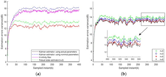
Figure 1.
Case 1: The modeling error takes a fixed value of . (a) Estimation error variance. (b) Estimation performance under different moving-horizon sizes n.
In Figure 2, the values of vary across different experiments and are uniformly distributed in the interval . The estimator’s performance shows an improvement of approximately 0.74 dB compared to the previous method [26], as illustrated in Figure 2a. Moreover, the proposed estimator also outperforms the filter by about 0.34 dB. In Figure 2b, the estimation error variance decreases from 20.54 dB to 20.15 dB with increasing moving horizon size n.
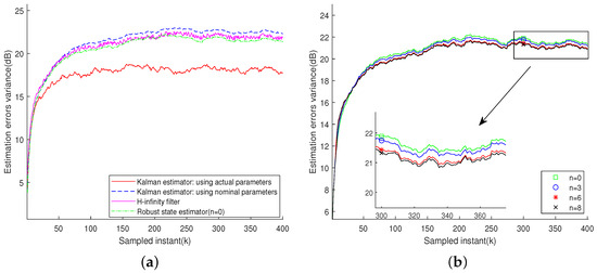
Figure 2.
Case 2: The modeling error in each experiment obeys a uniform distribution of [−1, 1]. (a) Estimation error variance. (b) Estimation performance under different moving-horizon sizes n.
To assess the robustness of the estimator under uncertainty, modeling errors , which vary at each sampling instant and follow a uniform distribution within the range , are introduced. As illustrated in Figure 3, the proposed robust state estimator consistently exhibits superior performance under these conditions.
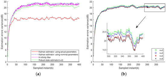
Figure 3.
Case 3: The modeling error in each moment obeys a uniform distribution of [−1, 1]. (a) Estimation error variance. (b) Estimation performance under different moving-horizon sizes n.
Figure 1, Figure 2 and Figure 3 illustrate that the proposed robust state estimator achieves consistently reliable estimation performance across different levels of parameter uncertainties. Moreover, the estimation error variance exhibits a decreasing trend as n increases, highlighting the method’s effectiveness. Furthermore, Table 1 summarizes the average estimation error covariance of different estimation algorithms over 400 simulation runs. Both the figures and the table validate the effectiveness of the designed robust estimator through performance demonstration.

Table 1.
Estimation Error Covariance Means (dB).
Table 1 summarizes the average estimation error covariance of different estimation algorithms over 400 simulation runs.
Moreover, the estimation error variance exhibits a decreasing trend as n increases, highlighting the method’s effectiveness. The figures and table confirm the effectiveness of the robust estimator.
It is worth emphasizing that, in this numerical example, the modeling uncertainty is intentionally introduced only in the state transition matrix , while the remaining system matrices are kept at their nominal values. This simplified setting is adopted to isolate the influence of parametric uncertainty and to clearly demonstrate the effectiveness of the proposed estimation strategy. It should be noted that the proposed framework itself is not restricted to second-order systems nor to uncertainties acting only on ; the theoretical formulation allows uncertainties to enter other system matrices as well, and the same derivation can be extended accordingly.
To quantify the impact of the uncertainty range on estimation accuracy, a scalar scaling factor is introduced such that , where . In this setting, represents a normalized, dimensionless parameter deviation, while controls the admissible magnitude of uncertainty around the nominal model, i.e., for all time instants k. This setting corresponds to practical time-varying systems in which parameters fluctuate within known bounded ranges.
The proposed estimator is evaluated for , while all other settings, including noise covariances, weighting matrices, and the horizon length fixed at , are kept unchanged. For each value of , the steady-state MMSE of the state estimate is computed, and the average results are reported in Table 2. As expected, the estimation error increases monotonically with . When , the estimator reduces to the nominal Kalman filter and achieves the minimum MMSE. As increases, the estimator remains stable but exhibits a gradual loss of accuracy due to the enlarged uncertainty set.
Table 2.
MMSE of the state estimate for different uncertainty scaling factors .
5. Conclusions
This work has established a robust state estimation framework for linear discrete-time systems with parametric uncertainties by embedding the RLS interpretation into the moving horizon estimation paradigm. Beyond algorithmic development, the main contribution lies in the theoretical characterization of the estimator’s long-term behavior. Specifically, the proposed formulation admits a recursive implementation with a Kalman filter-like structure, while guaranteeing the existence and uniqueness of a steady-state error covariance. It is further shown that the estimation error remains uniformly bounded in the mean-square sense and converges asymptotically to an unbiased estimate under bounded parametric perturbations.
In addition, the influence of the uncertainty range on estimation accuracy is explicitly investigated, revealing a monotonic relationship between the admissible parameter variation and the steady-state estimation error. This analysis provides a quantitative interpretation of robustness and clarifies the trade-off between uncertainty tolerance and estimation precision.
Future research will focus on extending the proposed theoretical framework to adaptive horizon selection mechanisms that preserve stability guarantees, as well as deriving tighter analytical bounds linking uncertainty magnitude to steady-state performance. Moreover, the applicability of the proposed estimator to non-autonomous (time-varying) systems will be investigated, with particular emphasis on establishing long-term stability and performance guarantees under time-dependent dynamics.
Author Contributions
Conceptualization, J.G. and H.L.; methodology, J.G.; software, J.G.; validation, H.L.; formal analysis, J.G.; investigation, J.G.; resources, H.L.; data curation, H.L.; writing—original draft preparation, J.G.; writing—review and editing, J.G.; visualization, H.L.; supervision, H.L.; project administration, H.L.; funding acquisition, H.L. All authors have read and agreed to the published version of the manuscript.
Funding
This research was funded by the National Natural Science Foundation of China, Grant Number 62273189, and the Shandong Provincial Natural Science Foundation, Grant Number ZR2020MF064.
Data Availability Statement
The data that support the findings of this study are available from the corresponding author upon reasonable request.
Conflicts of Interest
The authors declare no conflicts of interest.
Abbreviations
The following abbreviations are used in this manuscript:
| MHE | Moving Horizon Estimation |
| RLS | Recursive Least Square |
| MMSE | Minimum mean square error |
Appendix A
Based on Lemma 1 and the parameter modification in Equation (10), the following expression is obtained:
Using Lemma 1, Equation (A3) can be derived.
By invoking Lemma 1 and further simplifying Equation (A4), the following expression is obtained:
By applying the variable definitions in Equation (13), is reformulated as follows.
References
- Ma, F.; Liu, F.; Zhang, X.; Wang, P.; Bai, H.; Guo, H. An ultrasonic positioning algorithm based on maximum correntropy criterion extended Kalman filter weighted centroid. Signal Image Video Process. 2018, 12, 1207–1215. [Google Scholar] [CrossRef]
- Liu, X.; Zhang, Y.; Liu, D.; Wang, Q.; Bai, O.; Sun, J.; Rolfe, P. Physiological interference reduction for near infrared spectroscopy brain activity measurement based on recursive least squares adaptive filtering and least squares support vector machines. Comput. Assist. Surg. 2019, 24, 160–166. [Google Scholar] [CrossRef]
- Ahwiadi, M.; Wang, W. An adaptive particle filter technique for system state estimation and prognosis. IEEE Trans. Instrum. Meas. 2020, 69, 6756–6765. [Google Scholar] [CrossRef]
- Rocha, K.D.T.; Terra, M.H. Robust Kalman filter for systems subject to parametric uncertainties. Syst. Control Lett. 2021, 157, 105034. [Google Scholar] [CrossRef]
- He, X.; Xue, W.; Fang, H.; Hu, X. Consistent Kalman filters for nonlinear uncertain systems over sensor networks. Control Theory Technol. 2020, 18, 399–408. [Google Scholar] [CrossRef]
- He, D.; Xu, C.; Zhu, J.; Du, H. Moving horizon H∞ estimation of constrained multisensor systems with uncertainties and fading channels. IEEE Trans. Instrum. Meas. 2021, 70, 1–12. [Google Scholar] [CrossRef]
- Fu, M.; de Souza, C.E.; Xie, L. H∞ estimation for uncertain systems. Int. J. Robust Nonlinear Control 1992, 2, 87–105. [Google Scholar] [CrossRef]
- Milde, W.; Kerle, L. Comparison of Kalman filter and H-infinity filter for battery state of charge estimation with a detailed validation method. Batteries 2025, 11, 161. [Google Scholar] [CrossRef]
- Xu, D.; Qin, Y.; Zhang, H.; Yu, L.; Wang, H. Set-valued Kalman filtering: Event-triggered communication with quantized measurements. Peer-to-Peer Netw. Appl. 2019, 12, 677–688. [Google Scholar] [CrossRef]
- Meslem, N.; Hably, A.; Wang, Z.; Raïssi, T. Set-valued state estimator with sparse and delayed measurements for uncertain discrete-time linear systems. IEEE Control Syst. Lett. 2024, 8, 1234–1239. [Google Scholar] [CrossRef]
- Wang, F.; Wang, Z.; Liang, J.; Liu, X. Resilient state estimation for 2-D time-varying systems with redundant channels: A variance-constrained approach. IEEE Trans. Cybern. 2019, 49, 2479–2489. [Google Scholar] [CrossRef] [PubMed]
- Mahmoud, M.S.; Shi, P. Optimal guaranteed cost filtering for Markovian jump discrete-time systems. Math. Probl. Eng. 2004, 2004, 33–48. [Google Scholar] [CrossRef]
- Sayed, A.H. A framework for state-space estimation with uncertain models. IEEE Trans. Autom. Control 2001, 46, 998–1013. [Google Scholar] [CrossRef]
- Xu, H.; Mannor, S. A Kalman filter design based on the performance/robustness tradeoff. IEEE Trans. Autom. Control 2009, 54, 1171–1175. [Google Scholar]
- Ishihara, J.Y.; Terra, M.H.; Cerri, J.P. Optimal robust filtering for systems subject to uncertainties. Automatica 2015, 52, 120–130. [Google Scholar] [CrossRef]
- Liu, H.; Zhou, T. Robust state estimation for uncertain linear systems with random parametric uncertainties. Sci. China Inf. Sci. 2017, 60, 012202. [Google Scholar] [CrossRef]
- Rao, C.V.; Rawlings, J.B.; Lee, J.H. Constrained linear state estimation—A moving horizon approach. Automatica 2001, 37, 1619–1628. [Google Scholar] [CrossRef]
- Fujimoto, K.; Watanabe, T.; Hashimoto, Y.; Nishida, Y. Stochastic moving horizon estimation for linear discrete-time systems with parameter variation. In Proceedings of the 52nd IEEE Conference on Decision and Control, Firenze, Italy, 10–13 December 2013; pp. 5674–5679. [Google Scholar]
- Wang, Z.; Liu, Z.; Yuan, S.; Li, G. Adaptive horizon size moving horizon estimation with unknown noise statistical properties. Meas. Sci. Technol. 2024, 35, 116132. [Google Scholar] [CrossRef]
- Zhou, T.; Liang, H.Y. On asymptotic behaviors of a sensitivity penalization based robust state estimator. Syst. Control Lett. 2011, 60, 174–180. [Google Scholar] [CrossRef]
- Kailath, T.; Sayed, A.H.; Hassibi, B. Linear Estimation; Prentice Hall: Upper Saddle River, NJ, USA, 2000. [Google Scholar]
- Zhou, T. Sensitivity penalization based robust state estimation for uncertain linear systems. IEEE Trans. Autom. Control 2010, 55, 1018–1024. [Google Scholar] [CrossRef]
- Zhou, K.; Doyle, J.C.; Glover, K. Robust and Optimal Control; Prentice Hall: Hoboken, NJ, USA, 1996; p. 40. [Google Scholar]
- Du, X.; Liu, H.; Yu, H.; Huang, K. Robust fusion estimation under data-driven transmission strategy for multisensor systems with random packet drops. IEEE Trans. Instrum. Meas. 2024, 73, 1–11. [Google Scholar] [CrossRef]
- Zhang, Z.; Mao, Y.; Gao, J.; Liu, H. State estimation of discrete-time T–S fuzzy systems based on robustness ideas. Int. J. Fuzzy Syst. 2023, 25, 2007–2019. [Google Scholar] [CrossRef]
- Sinopoli, B.; Schenato, L.; Franceschetti, M.; Poolla, K.; Jordan, M.I.; Sastry, S.S. Kalman filtering with intermittent observations. IEEE Trans. Autom. Control 2004, 49, 1453–1464. [Google Scholar] [CrossRef]
Disclaimer/Publisher’s Note: The statements, opinions and data contained in all publications are solely those of the individual author(s) and contributor(s) and not of MDPI and/or the editor(s). MDPI and/or the editor(s) disclaim responsibility for any injury to people or property resulting from any ideas, methods, instructions or products referred to in the content. |
© 2026 by the authors. Licensee MDPI, Basel, Switzerland. This article is an open access article distributed under the terms and conditions of the Creative Commons Attribution (CC BY) license.