A Forecasting Model for Passenger Flows of Urban Rail Transit Based on Multi-Source Spatio-Temporal Features and Optimized Ensemble Learning

Abstract

In this study, we propose a novel model based on multi-source spatio-temporal features and optimized ensemble learning for forecasting station- and line-level passenger flows of urban rail transit. First, we design a spatio-temporal feature engineering method to enhance the accuracy of forecasting using passenger flow features; the temporal features include periodic and lag effects and the spatial features cover spatio-temporal attention mechanisms, adjacency relationships in the network graph and station clustering features. Furthermore, an improved ensemble learning method based on Extra Randomized Trees (ExtraTrees) and Light Gradient Boosting Machine (LightGBM) is developed to forecast the station-level passenger flows using a weighted sum method in which a particle swarm optimization algorithm is adopted to determine the weights assigned to the forecasting results of the two models. Finally, ridge regression is adopted as the meta-learning model to forecast line-level passenger flows. We employed passenger flow data from three urban rail transit lines in Hangzhou to demonstrate the feasibility of the proposed model. The results indicate that it produces more accurate passenger flow forecasts at the station and line levels than benchmark models. Therefore, it can provide a solid support for optimizing the operations, management, and planning for both a single urban rail transit station and the entire network.

1. Introduction

In recent years, rapid urban expansion and increasing travel demands have resulted in severe traffic congestion in cities [1]. High-capacity and high-speed urban rail transit can provide comfortable and punctual service and has become an efficient solution to reduce urban traffic pressure [2]. In mega-metro systems such as Seoul’s subway, peak-period passenger flows often lead to severe overcrowding in transfer stations [3]. By the end of 2025, China’s urban rail transit systems consisted of 343 lines with a total length of 11,710.3 km, accommodating 33.24 billion passenger trips annually—a 3.1% year-on-year increase. Empirical studies also show that in rapidly urbanizing regions, average daily ridership intensity can exceed 3.6 million passengers per day on major lines, reflecting both network dependence and growth pressure on the metro infrastructure [4]. However, with the increases in passenger flows, urban rail systems are encountering several operational issues, including overcrowding during peak hours, slow passenger movement on the platforms and increasing safety hazards. All of these challenges highlight the demand for accurate forecasts of passenger flow in urban rail systems.

Passenger flow indicates the change in passenger numbers in urban rail transit stations and lines over time. An accurate forecast of passenger flow enables informed decision-making in the operation, management, and planning of an urban rail station, as well as the entire line (e.g., efficient passenger flow management of stations and train scheduling on the line). Therefore, forecasting plays an important role in improving the efficiency and reliability of urban transportation systems [5], benefitting people’s lives and sustainable city development.

The accuracy of forecasting passenger flows in urban rail transit at both the station and line level depends on the development of an effective model. However, passenger flow exhibits complex characteristics, such as nonlinearity and uncertainty, since it is influenced by multiple sources of information (e.g., daily commute patterns and weather conditions). Such characteristics make modeling the passenger flow in urban rail transit difficult. In this case, there is a great need for a forecasting model that can effectively capture the complexity of passenger flow [6,7,8]. Moreover, recent research has found that passenger flow forecasting remains challenging due to the highly nonlinear and stochastic nature of ridership dynamics, which are significantly influenced by temporal and spatial factors across urban rail networks [9].

2. Literature Review

2.1. Urban Expansion and Traffic Congestion

Rapid urbanization is reshaping travel demand and is a key cause of chronic congestion in metropolitan regions [10]. Liu et al. [11] argued that relieving this pressure requires integrated strategies—transit-oriented development, multimodal integration, and prioritizing public transit—to shift trips away from private cars. Zhou et al. [12] used a bi-level programming model to show that the location of transit-oriented development stations strongly affects travel behavior, multimodal network equilibrium, and thus congestion. Serdar Dindar [13] noted that passenger flows are highly complex, reflecting urban activities and spatio-temporal heterogeneity rather than just commute patterns or weather, while Wang et al. [14] found that after-work activities—residential, leisure, and secondary destinations—strongly shape metro arrival times, usage patterns, and peak loads. Gao et al. [15] showed that spatio-temporal variability and differences across population groups are crucial for assessing how land use and transport affect mobility. The rise of shared micromobility, when integrated with transit, further complicates passenger behavior and undermines traditional planning assumptions [16]. Panel data also indicate that as urban rail networks grow more structurally complex, the coordination between population distribution and line layout has a major impact on passenger flow dynamics [17].

Collectively, these studies show that urban traffic congestion is not just a consequence of a supply–demand imbalance but is a multifaceted phenomenon shaped by urban form, land use policies, multimodal integration, and changing travel behaviors. The success of mitigation strategies—such as transit-oriented development and shared mobility—depends on understanding these dynamics. This insight motivates an examination of how passenger flow characteristics reflect these complex urban interactions. In the following subsection, we review the literature on passenger flow characteristics and their determinants, providing the analytical basis for robust forecasting frameworks.

2.2. Passenger Flow Characteristics and Influencing Factors

Passenger flow characteristics involve complex interactions among passenger behavior, network structure, and the built environment. Yuan et al. [18] reviewed urban rail passenger flow assignment methods, identifying an evolution from graph-theoretic path assignment to advanced frameworks that account for travel heterogeneity, dynamic passenger–train matching, and AI-based approaches, thereby improving our understanding of flow distribution. Zeng et al. [19] used random forest models to study metro–bus transfers in Shanghai and found that the transfer time and bus routes were dominant influencers of peak-hour transfer behavior, while land-use mix was more influential off-peak, underscoring temporal differences in intermodal integration. Chen et al. [20] applied a multi-scale spatio-temporal geographically weighted regression model with 13 POI types using demographic data for Hangzhou, showing that business and residential variables strongly increased morning peak inbound flows, while scenic spots suppressed them and corporate variables had non-stationary effects—boosting weekday but reducing weekend passenger flow.

Recent empirical studies have further clarified how multiple factors shape passenger demand across space and time. Zhao et al. [21] used Lasso-multiscale geographically weighted regression on Hangzhou AFC data and found that the ultra-peak boarding time was mainly influenced by transportation, residential, and working land use and closeness centrality, whereas the ultra-peak boarding volume was shaped by residential, working, and healthcare land use, bus stop density, and transfer station status. All effects showed strong spatial heterogeneity between urban cores and suburbs. Liu et al. [22], using the GeoDetector model for Shanghai, showed that interactions between built environment variables and land-use diversity significantly boosted metro ridership, with food and beverage services most influential on weekdays and accommodation services most influential on weekends. Liu et al. [23] applied panel data methods in Beijing and confirmed the temporal heterogeneity of land-use effects: land-use density increases the number of commuters in the morning peak and generates commuter trips in the evening peak, while land-use diversity promotes trips over longer periods on non-weekdays. Zhang et al. [24] used an XGBoost-SHAP model with Tianjin metro data and found that diverse travel-related factors accounted for 59.8% and 61.3% of importance on weekends and holidays, respectively, and that residential land strongly interacted with office, shopping, leisure, and tourist attractions across different periods.

Collectively, these studies show that passenger flow is affected by an interplay of temporal patterns, spatial dependencies, land use, transfer behavior, and evolving passenger activities. The documented spatio-temporal heterogeneity—across time periods, station types, and network contexts, including varying built-environment effects, nonlinear thresholds, and strong interaction effects—highlights the need for forecasting models that capture both local variation and system-wide dependencies.

2.3. Forecasting Models

In response to the growing need for accurate passenger flow predictions, there is a substantial body of research devoted to developing forecasting models for urban rail transit. The existing approaches can be broadly categorized into two main classes—statistical models and machine learning methods—each with distinct strengths and limitations in capturing the underlying dynamics of passenger demand.

Common statistical forecasting models are autoregressive integrated moving average (ARIMA) models, seasonal ARIMA (SARIMA) models, state-space models, and gray models. Zhang et al. [25] employed an enhanced ARIMA model to forecast the passenger flow at Tianfu Square Station on the Chengdu urban rail transit network. Li et al. [26] extended the ARIMA—into SARIMA—by incorporating seasonal components to achieve a more effective model of periodically varying time series, and used the proposed model to forecast passenger flow on the Guangzhou-to-Zhuhai intercity railway. Liang et al. [27] integrated state-space models with the k-nearest neighbors algorithm to improve the accuracy of passenger flow forecasts for Changchun rail stations. Song et al. [28] also successfully employed a fractional-order gray model to forecast short-term traffic flows in the UK.

Although commonly used to forecast passenger flows in urban rail transit, the above statistical models are generally incapable of characterizing the nonlinearity and dynamics in passenger flow data, which reduces their accuracy and adaptability [29]. As an alternative, machine learning techniques have been extensively adopted to forecast passenger flows in urban rail transit. Due to their strong nonlinear approximation capability, these methods can be used to automatically extract the complex latent patterns and dynamic dependencies in passenger flow data. Therefore, compared to statistical models, they can better address the obvious uncertainty and nonlinearity of real-world passenger flow dynamics. Sun et al. [30] utilized a support vector machine (SVM) model to forecast passenger flows on the Beijing metro, developing an improved Categorical Boosting (CatBoost) model to forecast the monthly ridership [31]. Chuwang et al. [5] used several machine learning models, including XGBoost and AdaBoost, to estimate historical passenger flows in the Changsha urban rail transit network. Wang et al. [32] proposed an ensemble forecasting framework that incorporates a random forest model to better characterize the heterogeneity of urban rail transit stations in order to estimate the passenger flows at metro stations in Hangzhou.

As a core subdomain of machine learning, deep learning has also been widely employed in urban rail transit passenger flow forecasting considering its strong capability in automated feature extraction and sequence modeling. Among the deep learning methods, the long short-term memory (LSTM) network, an extension of recurrent neural networks (RNNs), is designed to capture the long-range temporal dependencies of time series and has been studied by many researchers. Lu et al. [33] developed an enhanced LSTM-based model to forecast passenger flows in the Shanghai rail transit network and demonstrated its performance by comparing it with the single LSTM model. Wang et al. [34] proposed a hybrid forecasting approach that combines LSTM and a bidirectional gated recurrent unit (BiGRU), verifying that the proposed hybrid approach can achieve a higher forecasting accuracy than that achieved using only LSTM or BiGRU. Furthermore, Liu et al. [7] used the bidirectional LSTM (BiLSTM) network—which can exploit the comprehensive bidirectional contextual information in time-series data—to forecast the passenger flows in the Hangzhou rail transit system. Deng et al. [35] employed a temporal convolutional network (TCN) to forecast passenger flows in the Suzhou metro. However, these approaches rely heavily on the temporal features of urban rail transit passenger flows to carry out forecasting while neglecting the mutual interdependency and spatial correlations existing among the stations in real-world urban rail transit systems [36], worsening their performance in passenger flow forecasting.

To address this weakness, recent studies have incorporated spatial information into forecasting models. Graph convolutional networks (GCNs) designed to address graph-structured data can effectively capture the spatial dependencies among the nodes in a graph and have thus been widely used in passenger flow forecasting for urban rail transit. Zhang et al. [37] developed a multi-GCN with gated recurrent units to model both the spatial and temporal correlations of metro passenger flows in Hangzhou and Shanghai. Zeng et al. [38] combined GCNs, attention mechanisms, and LSTM networks to forecast passenger flows in the Shenzhen and Hangzhou rail transit systems; in these models, the travel behavior and comprehensive spatio-temporal dependencies are more tightly coupled with the forecasting. Liu et al. [39] proposed a Dynamic Spatio-Temporal Graph Fusion Network (DSTGFN) to deeply extract and exploit the spatio-temporal patterns of the passenger flows in urban rail transit and applied it to the networks in Hangzhou and Shanghai. Zeng et al. [40] introduced an Adaptive Spatio-Temporal Hierarchical Network (ASTHN) for passenger flow forecasting, in which a spatio-temporal gated convolutional layer (ST-Gconv) that integrates dilated convolutions, gating mechanisms and adaptive graph convolutions was introduced to enhance the ability to capture the complex spatio-temporal dependencies in passenger flow data. Yin et al. [41] applied fast Fourier transform to identify latent periodicities in passenger flow time-series and incorporated attention mechanisms with adaptive graph convolutional networks to learn temporal dependencies and spatial patterns separately under distinct periodic regimes. Xie et al. [42] developed a DSTGFN with alternately stacked multi-time attention modules and verified its improved accuracy in forecasting the passenger flows of urban rail systems in Beijing, Shanghai, and Hangzhou.

2.4. Research Gaps and Contributions

Existing studies have made significant contributions to passenger flow forecasting in urban rail transit stations. However, there are still weaknesses, as shown below.

(1) Although deep learning methods (especially GCNs) have been utilized in existing studies, these studies have not fully explored the scope and granularity of spatio-temporal feature fusion. Moreover, the majority of these works rely on graph neural networks to capture static or dynamic spatial dependencies among neighboring stations; however, they have not used multi-level aggregated information or multi-scale periodic patterns in forecasting. This incomplete feature engineering results in a model that lacks the ability to learn complex dynamics, which restricts forecasting accuracy.

(2) Deep neural networks and their variants require large training datasets and precise hyperparameter tuning to achieve acceptable performance, and their generalization is reduced when the data distribution changes. On the contrary, decision tree-based ensemble models (e.g., random forests and gradient boosting) are typically more robust to noisy features and are more interpretable. Although some studies have combined heterogeneous models to enhance forecasting accuracy, most fusion strategies still rely on simple stacking or a combination based on fixed weights. Such strategies cannot reflect the evolving passenger flow patterns or the spatial structure of the urban rail transit network. As a result, these static fusion strategies cannot adaptively integrate the models, which reduces the forecasting accuracy.

(3) Existing studies did not simultaneously forecast station- and line-level passenger flows. Aggregating station-level forecasts to the line level allows for station-specific errors to transfer and accumulate and further leads to deviations in line-level estimations, leading to large discrepancies between the estimated and actual line-level passenger flows. At the same time, models that only forecast line-level passenger flows cannot provide station-level results. Joint forecasting can provide accurate passenger flows in both urban rail transit stations and lines, which enables better operational, management and planning decisions. However, this has not been highlighted in the literature.

To address these issues, in this study, a passenger flow forecasting model for urban rail transit is proposed that combines multi-source spatio-temporal features and optimized ensemble learning. This study address deficiencies in the current research; its main contributions are as follows.

(1) To address inadequate feature fusion, we propose a multi-source spatio-temporal feature engineering framework to mine the multi-level heterogeneous space–time features of passenger flows in urban rail transit. This framework uses graph-based station adjacency and attention mechanisms to determine inter-station dependencies, clustering stations based on passenger flows. Furthermore, it incorporates diverse time variables (e.g., daily and weekly cycles) and lagged terms to capture the autocorrelation in passenger flow time-series.

(2) A dynamically weighted ensemble forecasting framework with high computational efficiency, a low training cost and improved numerical stability is proposed, in which ExtraTrees and LightGBM—models suitable for structured data—are used as base learners to calculate preliminary forecasts. A particle swarm optimization (PSO) algorithm is also adopted to determine their optimal aggregation weights to obtain the station-level forecasting results. This framework preserves the stability and interpretability of ensemble learning, and the contributions of the base learners can be adaptively adjusted to address the varying data distributions. Therefore, the overall accuracy and robustness of forecasting can be improved.

(3) To address the inconsistencies between station- and line-level passenger flow forecasting in urban rail transit, we developed a collaborative forecasting mechanism using ridge regression as the meta learner. During ridge regression, station- and line-level passenger flow forecasting is integrated within a unified optimization framework. At the meta-learning stage, it establishes relationships between the station- and line-level passenger flows to achieve joint forecasting optimization at the two levels.

3. Problem Description

Passenger flow data from rail transit stations are recorded sequentially in continuous time intervals to form a time series. Therefore, passenger flow forecasting of urban rail transit is a time-series forecasting problem, where historical data and explanatory variables are used to determine future values. The input of the forecasting model is the historical passenger flow sequences and the exogenous factors influencing the passenger flow, and its output is the future passenger flow.

The set of rail transit stations is represented by $=\left\{\mathrm{1,2},\dots ,N\right\}$, where $N$ is the total number of stations, $x_{i,t}$ represents the actual passenger flow of urban rail transit station $i$ at time $t$, and ${\widehat{x}}_{i,t}$ denotes its forecasting value. The objective of passenger flow forecasting for urban rail transit station $s_i$ is to build a function $f_i$, as shown in Equation (1), that minimizes the forecasting error $\left|x_{i,t}-{\widehat{x}}_{i,t}\right|$ across all training samples.

$${\widehat{x}}_{i,t}=f_i\left(x_{i,t-1},x_{i,t-2},\dots ,x_{i,t-L},x_{i,t-1}^{*},x_{i,t-2}^{*},\dots ,x_{i,t-L}^{*}\right)$$

(1)

where $L$ is the length of the historical data sequence and $x_{i,t}^{*}$ denotes the external feature vector influencing the passenger flow of urban rail transit station $i$ at time $t$.

Let $X_t^{\mathrm{l}\mathrm{i}\mathrm{n}\mathrm{e}}$ denote the line-level passenger flow at time $t$, and let ${\widehat{X}}_t^{\mathrm{l}\mathrm{i}\mathrm{n}\mathrm{e}}$ be the forecasting value. The function $F_t$ that forecasts the line-level passenger flow at time $t$ can be expressed in Equation (2), where $x_t=\left[x_{1,t},x_{2,t},\dots ,x_{N,t},x_{1,t}^{*},x_{2,t}^{*},\dots ,x_{N,t}^{*}\right]$.

$${\widehat{X}}_t^{\mathrm{line}}=F_t\left(x_{t-1},x_{t-2},\dots ,x_{t-L}\right)$$

(2)

Passenger flows within urban rail transit have the following complex characteristics that make forecasting difficult:

(1) Passenger flows exhibit complex temporal patterns and strong non-stationarity, including long-term trends, multiple seasonalities and irregular fluctuations. These components are nonlinear and time-varying and influence each other. A single forecasting model cannot sufficiently address this complexity and its forecasting accuracy is hence reduced.

(2) Passenger flows are influenced by the multi-source spatio-temporal factors that shape their spatial distributions and temporal evolutions. Such factors include calendar effects (e.g., weekdays, weekends and holidays), station interactions (e.g., passenger transfers), and station functions (e.g., transit hub or commercial center). These factors interact with each other in a complex way, which makes the feature engineering of passenger flow patterns and designing forecasting models difficult.

(3) Multi-level forecasting has consistency issues. The operations, management, and planning teams within urban rail transit systems require support from both station- and line-level passenger flow forecasts. However, existing forecasting methods are only suitable for only one or the other and cannot deal with simultaneous forecasting at both levels.

4. Model Construction

To address the above difficulties, we propose a model that integrates multi-source spatio-temporal features and features optimized ensemble learning. The model sequentially performs spatio-temporal feature engineering, dynamically weighted ensemble forecasting, and meta-learning-based fusion to obtain station- and line-level passenger flow forecasts.

Multi-source spatio-temporal feature engineering is the core of the proposed model. It can perform forecasting using multiple passenger flow features to enhance the accuracy of the results. This feature engineering employs temporal feature extraction to characterize the temporal dependencies and periodic regularities in the passenger flows in urban rail transit. Empirical observations show that these passenger flows exhibit evident cyclical fluctuations, including distinct morning and evening peaks on weekdays and significant differences in the passenger flows between weekdays and weekends. Additionally, the passenger flow at a given time is strongly correlated with that observed at temporally adjacent intervals [43]. All of these regularities influence passenger flow forecasting. To formulate these regularities in forecasts, the proposed model features the following two principal temporal features:

(1) Temporal periodic features that encode recurring cyclical patterns.

(2) Lag features that quantify the influence of the temporally adjacent historical observations on the target value.

These spatial features were constructed to characterize the complex interaction patterns among urban rail transit stations. The passenger flow at a given station is influenced by multiple factors (e.g., geographical location and station functions), and the resulting spatial effects on forecasting can be mainly classified into the following two categories:

(1) Propagation and diffusion of passenger flows between adjacent or spatially proximate urban rail transit stations.

(2) Coordinated variations that might occur between geographically distant urban rail transit stations due to similarities in functions and structural or operational characteristics [44].

To address the spatial effects, we propose the following three spatial features:

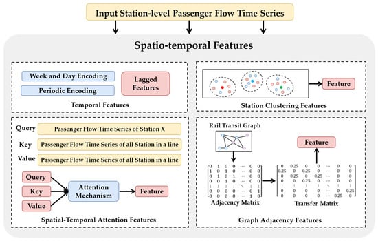
(1) Graph adjacency features to encode the urban rail network topology with an adjacency matrix derived from the physical connections among urban rail transit stations and lines [43]. This adjacency matrix is a binary matrix, where 1 indicates a direct connection between two stations and 0 indicates no direct connection. Accordingly, we can obtain a transfer matrix where each element represents the transfer probability of passenger flows between stations.

(2) Graph adjacency features alone cannot capture all spatial correlations, since non-contiguous stations might appear with strong interdependencies due to large events, key transfer hubs, or recurrent commuting patterns [45]. Attention-based features are adopted in the proposed model to deal with this issue. Through such features, the query, key, and value are derived from the passenger flow. The key and value are set as identical to represent the same spatio-temporal state. The attention-based features are designed to infer and quantify the dynamic correlations between each pair of urban rail transit stations at a given temporal scale to overcome the rigidity of the static graph structures.

(3) Passenger flow evolution strongly depends on the function of a station [46,47]. To represent this, stations are grouped by their passenger flow profiles into clusters that reflect similar functions and passenger flow characteristics. Each station is then assigned a cluster label, which allows the forecasting model to distinguish station types and adapt to the flow dynamics.

The overall multi-source spatio-temporal feature engineering process is illustrated in Figure 1.

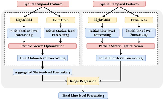
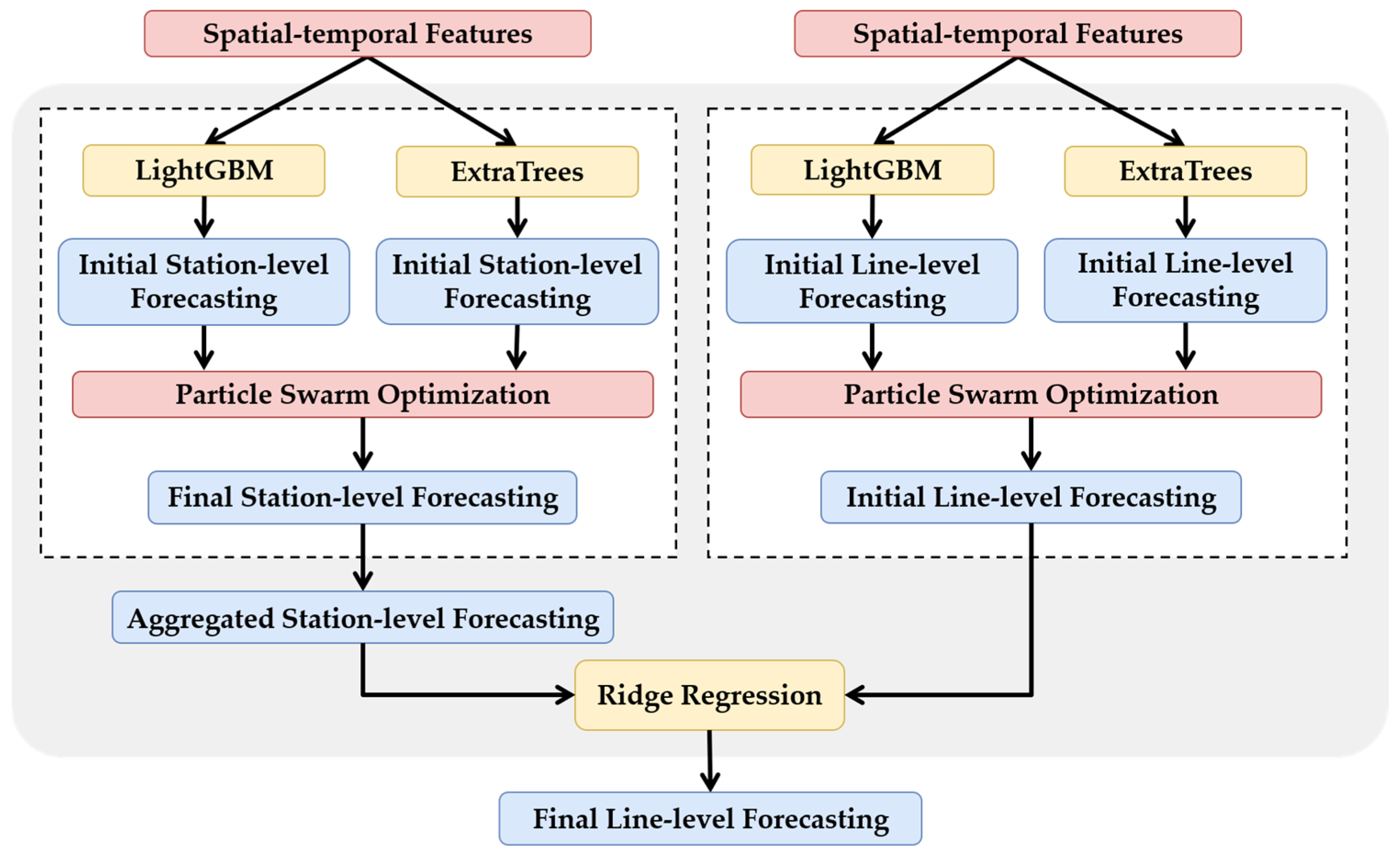
We further established an ensemble learning model to overcome the single model’s lack of ability to jointly forecast noisy, nonlinear station- and line-level passenger flows that are influenced by multiple factors [48]. We used ExtraTrees and LightGBM as the base models to build an ensemble learning model, since the former can avoid data overfitting and handle data uncertainty [49] and the latter can model complex nonlinear relationships and feature interactions [50]. The optimized ensemble learning outputs the forecasting results via the following procedure.

First, the station-level passenger flow for each station is initially forecasted by the two base models using the spatio-temporal features as inputs. We then employ the PSO algorithm to search for the optimal fusion weights of ExtraTrees and LightGBM to obtain the final forecasts, in which the robustness and accuracy are balanced.

Then, we sum the results of all stations in a line to obtain the aggregated station-level passenger flow forecasts. This process provides a bottom-up estimation of a line’s entire passenger demand while preserving station-level heterogeneity and enabling a line-wide analysis.

The initial line-level passenger flow can be forecasted by the ensemble learning model using the aggregated station-level passenger flows as training data, which enables line-wide temporal patterns, inter-station dynamics, and holistic line-level passenger flow trends to be captured.

Finally, we introduce a meta-learning fusion step to achieve an accurate final forecast. Ridge regression exhibits the advantages of reducing overfitting and handling multicollinearity among input features [51]. Therefore, we employed it as the meta-learner in this step to forecast the final line-level passenger flow, taking the initial line-level and aggregated station-level passenger flow forecasts as the inputs.

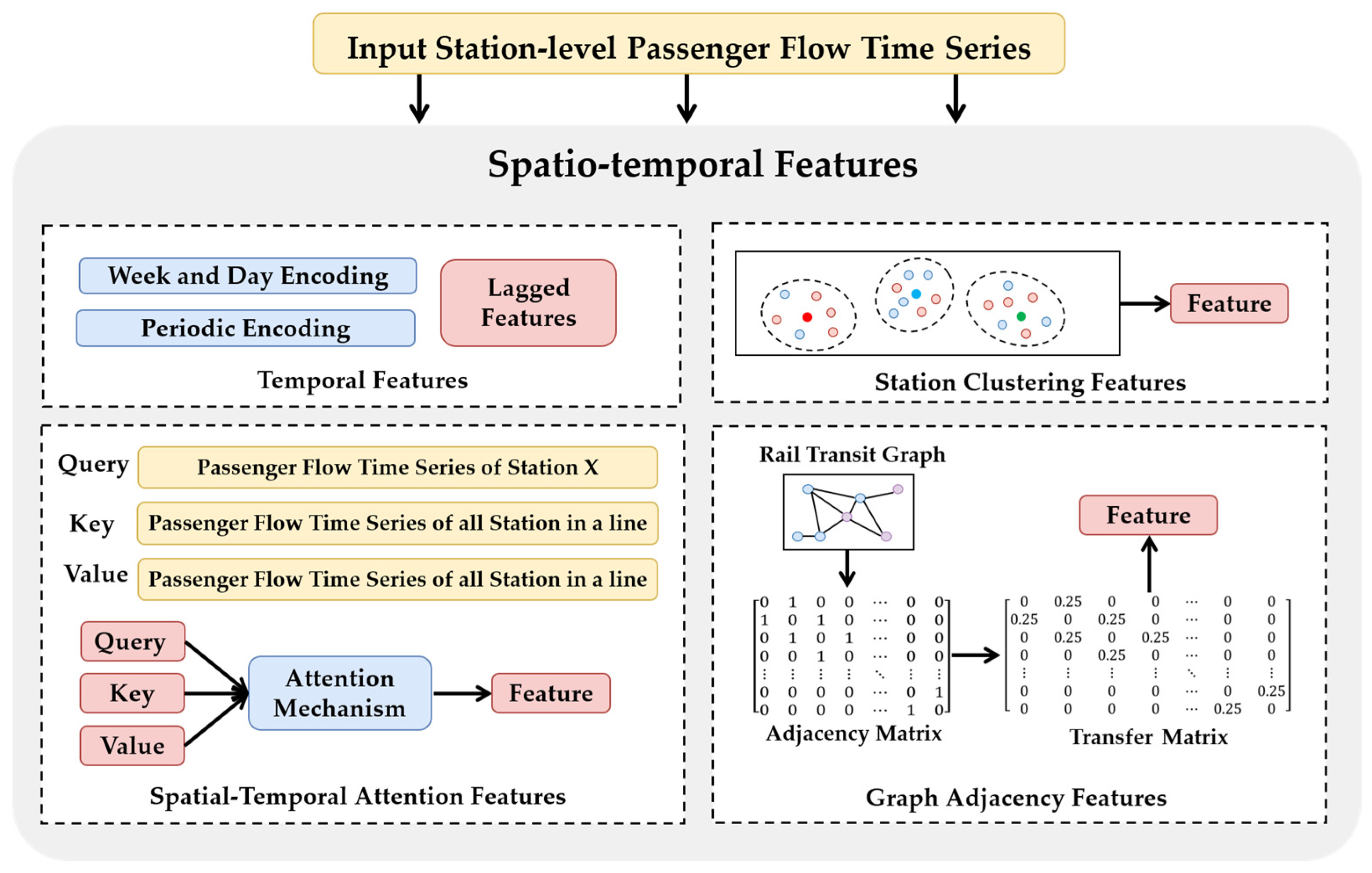
The overall forecasting process of the ensemble learning model is shown in Figure 2.

4.1. Temporal Features

Temporal features can either be discrete or continuous. The former are derived directly from timestamps, and include $t_{\mathrm{week}}$—the feature that captures weekly patterns—and $t_{\mathrm{hour}}$—the feature that reflects daily variations.

However, discrete features cannot represent cyclical variations. Therefore, we used the continuous periodic features to map the actual time into a cyclic space using sine and cosine functions. This ensures that the same times on different days have the same representation, helping the model recognize and leverage repeated patterns across different time points. In this encoding, times near midnight remain close in the cyclic space so the discontinuity of discrete hour or minute indicators is avoided. By mapping time to a unit circle with two continuous features, the model captures the periodic patterns of daily passenger flows. Specifically, time $t$ is first converted into a real number (e.g., 3:30 p.m. is converted into 930), and then transformed by Equation (3) into sine and cosine values:

$$\left\{\begin{array}{c}{t}_{\mathrm{s}\mathrm{i}\mathrm{n}}=\mathrm{s}\mathrm{i}\mathrm{n}\left({\displaystyle \frac{2\pi t}{T_{\mathrm{day}}}}\right)\\ t_{\mathrm{c}\mathrm{o}\mathrm{s}}=\mathrm{c}\mathrm{o}\mathrm{s}\left({\displaystyle \frac{2\pi t}{T_{\mathrm{day}}}}\right)\end{array}\right.$$

(3)

where $t_{\mathrm{s}\mathrm{i}\mathrm{n}}$ and $t_{\mathrm{c}\mathrm{o}\mathrm{s}}$ are the sine and cosine representations of time $t$, respectively, and $T_{\mathrm{day}}$ is the total minutes in a day (i.e., 1440).

Lagged features identify short-term temporal dependences in passenger flows. Lag feature vector ${\mathrm{l}\mathrm{a}\mathrm{g}}_{i,t}$ for station $i$ at time $t$ was employed to capture the recent passenger flow, and is formulated in Equation (4):

$${\mathrm{l}\mathrm{a}\mathrm{g}}_{i,t}=[x_{i,t-1},x_{i,t-2},x_{i,t-3},x_{i,t-4},\dots ,x_{i,t-L}]$$

(4)

where $L$ denotes the lag length. Missing values at the start of ${\mathrm{l}\mathrm{a}\mathrm{g}}_{i,t}$ are padded with zeros. Finally, all temporal features of station $i$ at time $t$ are concatenated into a complete temporal feature vector ${\mathrm{f}\mathrm{e}\mathrm{a}\mathrm{t}\mathrm{u}\mathrm{r}\mathrm{e}}_{i,t}^{\mathrm{time}}$, as shown in Equation (5):

$${\mathrm{f}\mathrm{e}\mathrm{a}\mathrm{t}\mathrm{u}\mathrm{r}\mathrm{e}}_{i,t}^{\mathrm{time}}=[t_{\mathrm{s}\mathrm{i}\mathrm{n}},t_{\mathrm{c}\mathrm{o}\mathrm{s}},t_{\mathrm{week}},t_{\mathrm{hour}},{\mathrm{l}\mathrm{a}\mathrm{g}}_{i,t}]$$

(5)

4.2. Spatial Features

4.2.1. Spatio-Temporal Attention Features

To capture spatio-temporal dependencies, we dynamically weighted the historical passenger flows across all the stations using an attention mechanism. This weight indicates the relevance of historical passenger flows to current passenger flow, which can be further used by the model. Unlike moving averages using fixed weights, the attention mechanism assigns weights based on the above relevance, and therefore the weights can be allocated more reasonably.

The historical passenger flow matrix at time $t$ is represented by Equation (6):

$$P_t=[X_{t-\mathrm{l}\mathrm{e}\mathrm{n}+1},X_{t-\mathrm{l}\mathrm{e}\mathrm{n}+2},\dots ,X_t]$$

(6)

where $X_t$ is a row vector of the passenger flows for all stations at time $t$, $\mathrm{l}\mathrm{e}\mathrm{n}$ represents the length of the attention window, and $X_t=\left[x_{1,t},x_{2,t},x_{3,t},\dots ,x_{N,t}\right]$.

We took the last row of $P_t$ as the query vector $Q_t$ at time $t$, i.e., $Q_t=X_t$, and used $P_t$ as both the key matrix $K_t$ and value matrix $V_t$ at time $t$, i.e., $Q_t=X_t$, $K_t=P_t$ and $V_t=P_t$. The attention score, that is, the scaled dot product, is computed by Equation (7):

$${\mathrm{score}}_t={\displaystyle \frac{Q_t{K}_t^{\mathrm{\top }}}{\sqrt{d_k}}}$$

(7)

where $d_k$ is the dimension of the key matrix.

To ensure numerical stability, we subtracted the maximum value of the attention score, as shown in Equation (8):

$${\mathrm{score}}_t^{\prime }={\mathrm{score}}_t-\mathrm{m}\mathrm{a}\mathrm{x} \left({\mathrm{score}}_t\right).$$

(8)

Attention weight ${\alpha }_t$ represents the importance of historical passenger flows within the window of the current forecast, and is obtained by Equation (9):

$${\alpha }_t=\mathrm{softmax}\left({\mathrm{score}}_t^{\prime }\right)=\left[{\displaystyle \frac{\mathrm{e}\mathrm{x}\mathrm{p} \left({\mathrm{score}}_{1,t}^{\prime }\right)}{\sum _{h=1}^{\mathrm{l}\mathrm{e}\mathrm{n}}\mathrm{e}\mathrm{x}\mathrm{p} ({\mathrm{score}}_{h,t}^{\prime })}},\dots ,{\displaystyle \frac{\mathrm{e}\mathrm{x}\mathrm{p} \left({\mathrm{score}}_{\mathrm{l}\mathrm{e}\mathrm{n},t}^{\prime }\right)}{\sum _{h=1}^{\mathrm{l}\mathrm{e}\mathrm{n}}\mathrm{e}\mathrm{x}\mathrm{p} ({\mathrm{score}}_{h,t}^{\prime })}}\right]$$

(9)

where $h$ denotes the index of the historical passenger flow matrix at time $t$. The final attention output is a weighted sum of the value matrix, as shown in Equation (10):

$${\mathrm{a}\mathrm{t}\mathrm{t}\mathrm{e}\mathrm{n}\mathrm{t}\mathrm{i}\mathrm{o}\mathrm{n}}_t={\alpha }_t{V}_t^{\mathrm{T}}$$

(10)

where ${\mathrm{a}\mathrm{t}\mathrm{t}\mathrm{e}\mathrm{n}\mathrm{t}\mathrm{i}\mathrm{o}\mathrm{n}}_t=[{\mathrm{a}\mathrm{t}\mathrm{t}\mathrm{e}\mathrm{n}\mathrm{t}\mathrm{i}\mathrm{o}\mathrm{n}}_{1,t},{\mathrm{a}\mathrm{t}\mathrm{t}\mathrm{e}\mathrm{n}\mathrm{t}\mathrm{i}\mathrm{o}\mathrm{n}}_{2,t},\dots ,{\mathrm{a}\mathrm{t}\mathrm{t}\mathrm{e}\mathrm{n}\mathrm{t}\mathrm{i}\mathrm{o}\mathrm{n}}_{N,t}]$, in which ${\mathrm{a}\mathrm{t}\mathrm{t}\mathrm{e}\mathrm{n}\mathrm{t}\mathrm{i}\mathrm{o}\mathrm{n}}_{i,t}$ represents the adaptively weighted value of passenger flow for station $i$ at time $t$.

4.2.2. Graph Adjacency Features

The graph adjacency features are determined by the connectivity of the urban rail transit network, and can thus simulate passenger flow propagation between the stations in the network. Passenger flow moves between two adjacent stations or lines, which has an influence on both stations’ individual flows. Modeling these relationships is crucial for passenger flow forecasting.

Spatial connectivity is encoded in an $N\times N$ adjacency matrix $A$, whose elements are given by Equation (11):

$$A_{i,j}=\left\{\begin{array}{cc}1,& \mathrm{if} \mathrm{station} i \mathrm{and} j \mathrm{are} \mathrm{directly} \mathrm{linked} \mathrm{by} \mathrm{track}\\ 0,& \mathrm{otherwise}\end{array}\right.$$

(11)

where $A_{i,j}=1$ represents a direct connection allowing passenger flow movement from $i$ to $j$. To represent flow, the transfer probability, $A$, is row-normalized to obtain an $N\times N$ transfer matrix. The transfer matrix ${\mathrm{t}\mathrm{r}\mathrm{a}\mathrm{n}\mathrm{s}\mathrm{f}\mathrm{e}\mathrm{r}}_{i,j}$ represents the transfer probabilities of passengers moving from station $i$ to station $j$, and is calculated by Equation (12):

$${\mathrm{t}\mathrm{r}\mathrm{a}\mathrm{n}\mathrm{s}\mathrm{f}\mathrm{e}\mathrm{r}}_{i,j}={\displaystyle \frac{A_{ij}}{\sum _{j=1}^N{A}_{ij}}}$$

(12)

After obtaining the one-step transfer matrix ${\mathrm{t}\mathrm{r}\mathrm{a}\mathrm{n}\mathrm{s}\mathrm{f}\mathrm{e}\mathrm{r}}_{i,j}$, we further leverage this matrix to capture the multi-step propagation of passenger flows. Let ${\mathrm{t}\mathrm{r}\mathrm{a}\mathrm{n}\mathrm{s}\mathrm{f}\mathrm{e}\mathrm{r}}^{\lambda }$ denote the matrix raised to power $\lambda$, and its elements ${\mathrm{t}\mathrm{r}\mathrm{a}\mathrm{n}\mathrm{s}\mathrm{f}\mathrm{e}\mathrm{r}}_{i,j}^{\lambda }$ represent the probability that the passenger flow moves from station $i$ to station $j$ in $\lambda$ steps. For a given $\lambda$, spatial propagation feature vector ${\mathrm{g}\mathrm{r}\mathrm{a}\mathrm{p}\mathrm{h}}_t^{\lambda }$ at time $t$ is given by Equation (13):

$${\mathrm{g}\mathrm{r}\mathrm{a}\mathrm{p}\mathrm{h}}_t^{\lambda }={\mathrm{f}\mathrm{l}\mathrm{o}\mathrm{w}}_{t-1}·{\mathrm{t}\mathrm{r}\mathrm{a}\mathrm{n}\mathrm{s}\mathrm{f}\mathrm{e}\mathrm{r}}^{\lambda }$$

(13)

where ${\mathrm{f}\mathrm{l}\mathrm{o}\mathrm{w}}_{t-1}=[x_{1,t-1},x_{2,t-1},\dots ,x_{N,t-1}]$ is the passenger flow vector of all stations at time $t-1$. The $\lambda$-th power spatial feature of station $i$ at time $t$ is determined by Equation (14):

$${\mathrm{g}\mathrm{r}\mathrm{a}\mathrm{p}\mathrm{h}}_{i,t}^{\lambda }=\sum _{o=1}^N{x}_{o,t-1}\cdot {\mathrm{t}\mathrm{r}\mathrm{a}\mathrm{n}\mathrm{s}\mathrm{f}\mathrm{e}\mathrm{r}}_{i,o}^{\lambda }$$

(14)

where $o$ denotes the index of the elements in ${\mathrm{f}\mathrm{l}\mathrm{o}\mathrm{w}}_{t-1}$, and ${\mathrm{g}\mathrm{r}\mathrm{a}\mathrm{p}\mathrm{h}}_{i,t}^{\lambda }$ represents the passenger flow arriving at station $i$ at time $t$ after $\mathsf{\lambda }$ steps.

4.2.3. Station Clustering Features

Urban rail transit stations are clustered based on passenger flows. This allows the model to use the shared characteristics of stations within the same cluster when forecasting passenger flows, which improves its generalization.

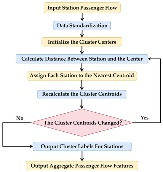
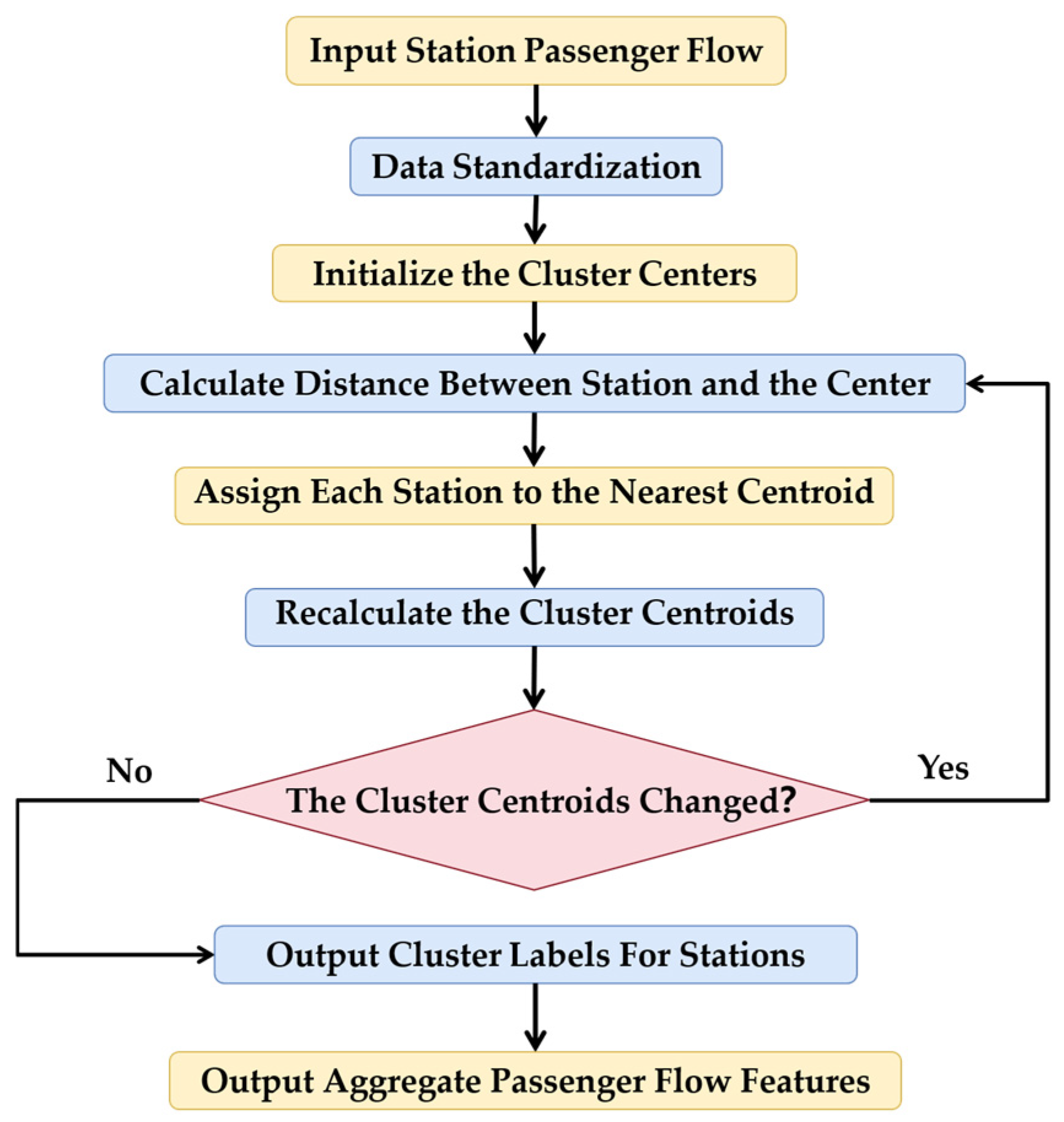
When constructing the spatial clustering features, the passenger flow of rail transit stations should first be standardized. The K-means algorithm should then be applied to group stations with similar passenger flow characteristics: after initializing cluster centers, each station is assigned to the nearest centroid based on the Euclidean distance, and centroids are recalculated until convergence. Upon completion, each station $i$ is assigned a final cluster label.

Based on the clustering result, two features are created for each station: (1) a cluster historical aggregate passenger flow ${\mathrm{label}}_{i,r}^{\mathrm{sum}}$, that is, the total passenger flow within the cluster label $r$ to which station $i$ belongs, and (2) a one-hot encoding vector ${\mathrm{l}\mathrm{a}\mathrm{b}\mathrm{e}\mathrm{l}}_i$ which identifies the cluster membership of station $i$.

The final output of this stage is a complete spatial feature vector for station $i$ at time $t$, formed by concatenating attention mechanism output ${\mathrm{a}\mathrm{t}\mathrm{t}\mathrm{e}\mathrm{n}\mathrm{t}\mathrm{i}\mathrm{o}\mathrm{n}}_{i,t}$, graph feature ${\mathrm{g}\mathrm{r}\mathrm{a}\mathrm{p}\mathrm{h}}_{i,t}^{\lambda }$, and the two cluster features:

$${\mathrm{f}\mathrm{e}\mathrm{a}\mathrm{t}\mathrm{u}\mathrm{r}\mathrm{e}}_{i,t}^{\mathrm{space}}=[{\mathrm{a}\mathrm{t}\mathrm{t}\mathrm{e}\mathrm{n}\mathrm{t}\mathrm{i}\mathrm{o}\mathrm{n}}_{i,t}, {\mathrm{g}\mathrm{r}\mathrm{a}\mathrm{p}\mathrm{h}}_{i,t}^p, {\mathrm{l}\mathrm{a}\mathrm{b}\mathrm{e}\mathrm{l}}_{i,r}^{\mathrm{s}\mathrm{u}\mathrm{m}}, {\mathrm{l}\mathrm{a}\mathrm{b}\mathrm{e}\mathrm{l}}_i]$$

(15)

The procedure of spatial clustering feature construction is shown in Figure 3.

4.3. Ensemble Learning

We developed a two-stage weighted ensemble framework to integrate the multi-source spatio-temporal features obtained in Section 4.1 and Section 4.2. In this way, reliable and stable passenger flow forecasts were obtained. In Stage 1, two base learners, ExtraTrees and LightGBM, were combined by using dynamically optimized weights to generate the initial station-level forecast. The input to each model was the spatio-temporal feature vector ${\mathrm{f}\mathrm{e}\mathrm{a}\mathrm{t}\mathrm{u}\mathrm{r}\mathrm{e}}_{i,t}$ of station $i$ at time $t$, which is presented in Equation (16). In Stage 2, a meta-learner, i.e., ridge regression, was employed to integrate the initial line-level forecast with the aggregated station-level forecasts to obtain a final line-level forecast.

$${\mathrm{f}\mathrm{e}\mathrm{a}\mathrm{t}\mathrm{u}\mathrm{r}\mathrm{e}}_{i,t}=[{\mathrm{f}\mathrm{e}\mathrm{a}\mathrm{t}\mathrm{u}\mathrm{r}\mathrm{e}}_{i,t}^{\mathrm{time}},{\mathrm{f}\mathrm{e}\mathrm{a}\mathrm{t}\mathrm{u}\mathrm{r}\mathrm{e}}_{i,t}^{\mathrm{space}}]$$

(16)

4.3.1. Base Model I: ExtraTrees

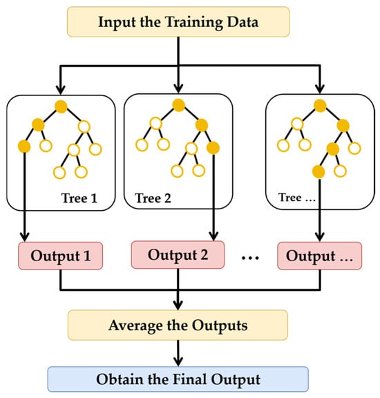
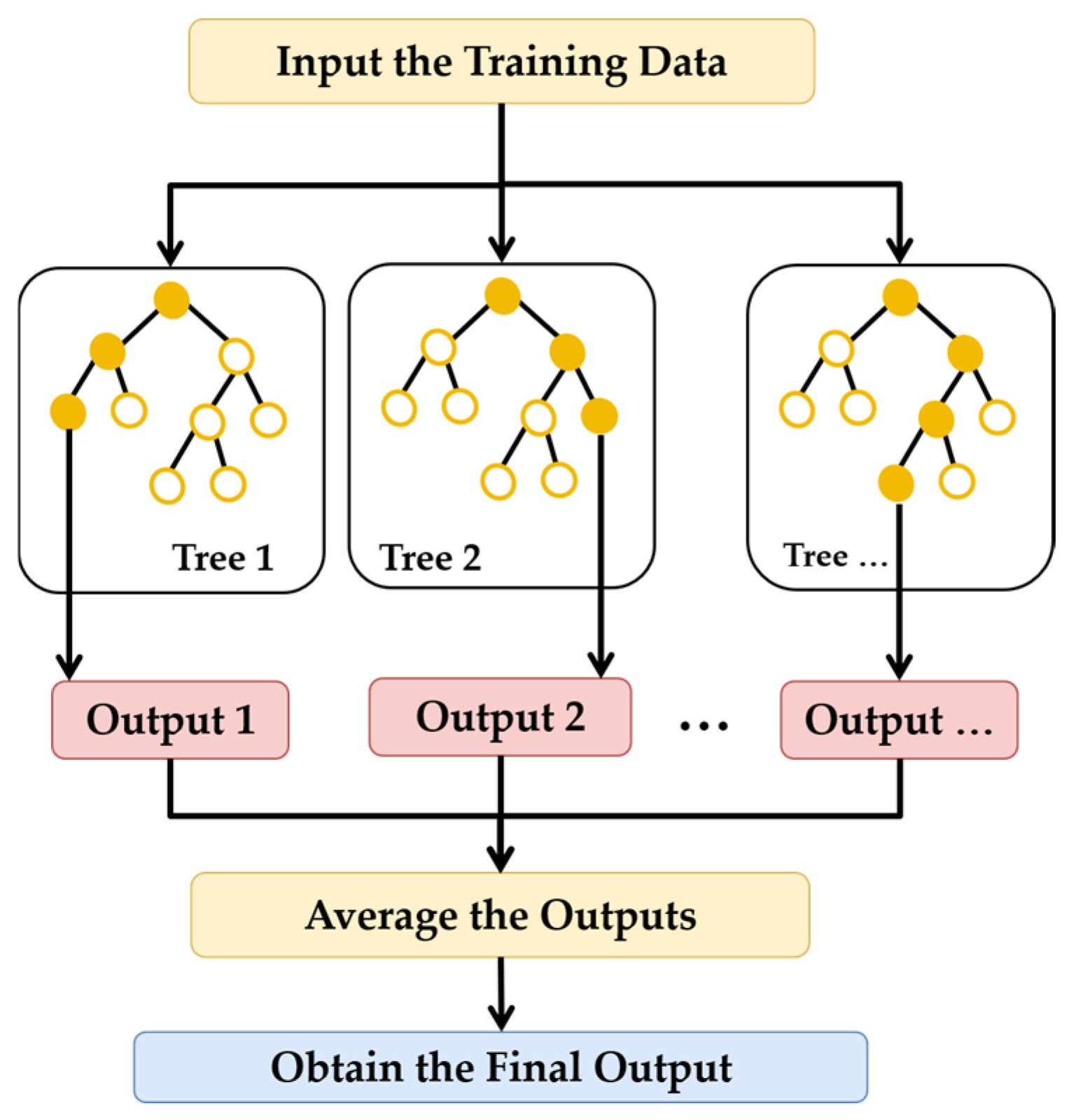
ExtraTrees is a highly randomized tree ensemble. It builds multiple decision trees by randomly selecting feature subsets and split points to carry out cooperative forecasting. Each tree is built with different feature and split choices. This randomness reduces variance and improves generalization. The structure of ExtraTrees is shown in Figure 4.

The final station-level forecasting result of station $i$ at time $t$ is the average output of all trees’ outputs, as shown in Equation (17):

$${\widehat{x}}_{i,t}^{\mathrm{E}\mathrm{x}\mathrm{t}\mathrm{r}\mathrm{a}\mathrm{T}\mathrm{r}\mathrm{e}\mathrm{e}\mathrm{s}}=\mathrm{E}\mathrm{x}\mathrm{t}\mathrm{r}\mathrm{a}\mathrm{T}\mathrm{r}\mathrm{e}\mathrm{e}\mathrm{s}({\mathrm{f}\mathrm{e}\mathrm{a}\mathrm{t}\mathrm{u}\mathrm{r}\mathrm{e}}_{i,t})$$

(17)

4.3.2. Base Model II: LightGBM

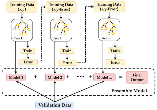
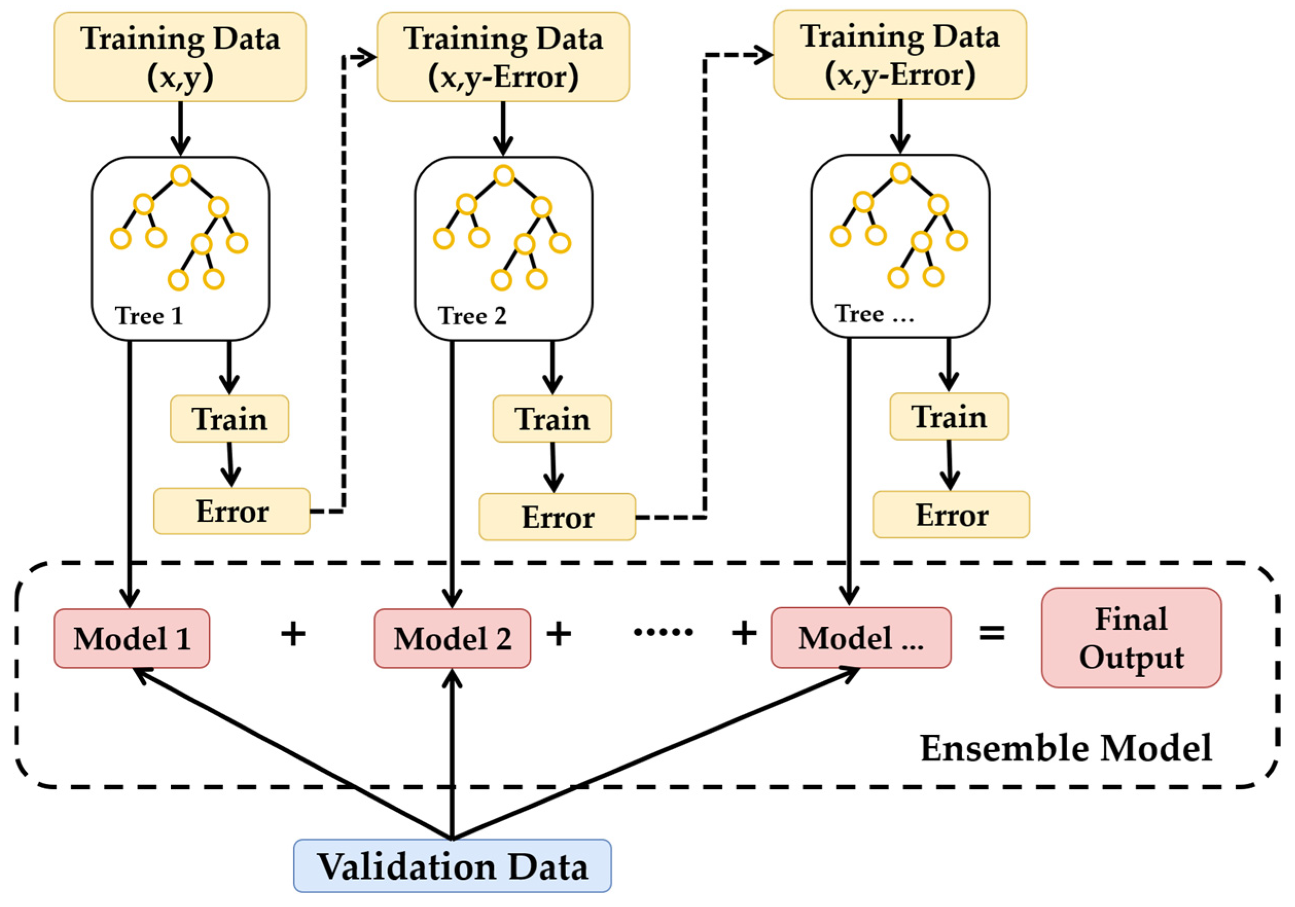
LightGBM is an efficient gradient-boosting framework. It grows trees sequentially, and each new tree is trained to correct the residual errors of the current ensemble. LightGBM uses histogram-based algorithms to achieve a fast training speed and a leaf-wise growth strategy to achieve high accuracy. Therefore, it is suitable for processing large amounts of data. The structure of LightGBM is shown in Figure 5.

The station-level passenger flow forecast for station $i$ at time $t$ is given by Equation (18):

$${\widehat{x}}_{i,t}^{\mathrm{L}\mathrm{i}\mathrm{g}\mathrm{h}\mathrm{t}\mathrm{G}\mathrm{B}\mathrm{M}}=\mathrm{L}\mathrm{i}\mathrm{g}\mathrm{h}\mathrm{t}\mathrm{G}\mathrm{B}\mathrm{M}({\mathrm{f}\mathrm{e}\mathrm{a}\mathrm{t}\mathrm{u}\mathrm{r}\mathrm{e}}_{i,t})$$

(18)

4.3.3. Dynamic Weight Optimization via the PSO Algorithm

The weighted combination of the two base models produces the final station-level forecast. The optimal weights are determined by minimizing the forecasting error of the validation set by using the PSO algorithm.

The validation set is denoted as ${\mathrm{D}\mathrm{a}\mathrm{t}\mathrm{a}}_{\mathrm{val}}=\{({\mathrm{f}\mathrm{e}\mathrm{a}\mathrm{t}\mathrm{u}\mathrm{r}\mathrm{e}}_{i,t},x_{i,t})\}$. The combined forecasting result ${\widehat{x}}_{i,t}^{\mathrm{b}\mathrm{a}\mathrm{s}\mathrm{e}}(w)$ using the weight vector $w=(w_{\mathrm{E}\mathrm{x}\mathrm{t}\mathrm{r}\mathrm{a}\mathrm{T}\mathrm{r}\mathrm{e}\mathrm{e}\mathrm{s}},w_{\mathrm{L}\mathrm{i}\mathrm{g}\mathrm{h}\mathrm{t}\mathrm{G}\mathrm{B}\mathrm{M}})$ is presented in Equation (19):

$${\widehat{x}}_{i,t}^{\mathrm{b}\mathrm{a}\mathrm{s}\mathrm{e}}(w)=w_{\mathrm{E}\mathrm{x}\mathrm{t}\mathrm{r}\mathrm{a}\mathrm{T}\mathrm{r}\mathrm{e}\mathrm{e}\mathrm{s}}\cdot {\widehat{x}}_{i,t}^{\mathrm{E}\mathrm{x}\mathrm{t}\mathrm{r}\mathrm{a}\mathrm{T}\mathrm{r}\mathrm{e}\mathrm{e}\mathrm{s}}+w_{\mathrm{L}\mathrm{i}\mathrm{g}\mathrm{h}\mathrm{t}\mathrm{G}\mathrm{B}\mathrm{M}}\cdot {\widehat{x}}_{i,t}^{\mathrm{L}\mathrm{i}\mathrm{g}\mathrm{h}\mathrm{t}\mathrm{G}\mathrm{B}\mathrm{M}}$$

(19)

where $w_{\mathrm{E}\mathrm{x}\mathrm{t}\mathrm{r}\mathrm{a}\mathrm{T}\mathrm{r}\mathrm{e}\mathrm{e}\mathrm{s}}$ and $w_{\mathrm{L}\mathrm{i}\mathrm{g}\mathrm{h}\mathrm{t}\mathrm{G}\mathrm{B}\mathrm{M}}$ are the weights assigned to the forecasting results given by ExtraTrees and LightGBM, respectively. The objective of Equation (20) is to find the optimal weight vector $w^{*}=(w_{\mathrm{E}\mathrm{x}\mathrm{t}\mathrm{r}\mathrm{a}\mathrm{T}\mathrm{r}\mathrm{e}\mathrm{e}\mathrm{s}}^{*},w_{\mathrm{L}\mathrm{i}\mathrm{g}\mathrm{h}\mathrm{t}\mathrm{G}\mathrm{B}\mathrm{M}}^{*})$ that minimizes the Root Mean Square Error (RMSE) of the validation set:

$$w^{*}=\mathrm{a}\mathrm{r}\mathrm{g} \underset{w}{\mathrm{m}\mathrm{i}\mathrm{n}}\sqrt{{\displaystyle \frac{1}{\mid {\mathrm{D}\mathrm{a}\mathrm{t}\mathrm{a}}_{\mathrm{val}}\mid }}\sum _{(i,t)\in {\mathrm{D}\mathrm{a}\mathrm{t}\mathrm{a}}_{\mathrm{val}}}{\left(x_{i,t}-{\widehat{x}}_{i,t}^{\mathrm{b}\mathrm{a}\mathrm{s}\mathrm{e}}(w)\right)}^2}$$

(20)

The PSO algorithm is employed to solve this optimization problem. A swarm of $M$ particles is initialized. At iteration $u$, each particle $m$ has a position vector $w_m^u$, which represents a candidate weight vector and a velocity vector $v_m^u$. Particles update their states based on their personal best position $w_{m,u}^{\mathrm{pbest}}$ and the swarm’s global best position $w_u^{\mathrm{gbest}}$, which are updated at each iteration $u$, as indicated by Equations (21) and (22):

$$v_m^{u+1}=\omega \cdot v_m^u+c_1{r}_1^u\left(w_{m,u}^{\mathrm{pbest}}-w_m^u\right)+c_2{r}_2^u\left(w_u^{\mathrm{gbest}}-w_m^u\right)$$

(21)

$$w_m^{u+1}=w_m^u+v_m^{u+1}$$

(22)

where $\omega$ is the inertia weight, $c_1$ and $c_2$ are acceleration coefficients, and $r_1^u$ and $r_2^u$ are random numbers that are uniformly distributed between 0 and 1. Upon convergence, the final global best position $w^{\mathrm{gbest}}$ is set as $w^{\mathrm{*}}$. Then, $w^{\mathrm{*}}=(w_{\mathrm{E}\mathrm{x}\mathrm{t}\mathrm{r}\mathrm{a}\mathrm{T}\mathrm{r}\mathrm{e}\mathrm{e}\mathrm{s}}^{\mathrm{*}},w_{\mathrm{L}\mathrm{i}\mathrm{g}\mathrm{h}\mathrm{t}\mathrm{G}\mathrm{B}\mathrm{M}}^{\mathrm{*}})$ is put into Equation (23) to normalize the weights to ensure the sum of their values is 1 in order to ensure that the relative contribution of each base learner is fully represented in the final station-level passenger flow forecast.

$$\left\{\begin{array}{c}{w}_{\mathrm{E}\mathrm{x}\mathrm{t}\mathrm{r}\mathrm{a}\mathrm{T}\mathrm{r}\mathrm{e}\mathrm{e}\mathrm{s}}^{\mathrm{normalize}}={\displaystyle \frac{w_{\mathrm{E}\mathrm{x}\mathrm{t}\mathrm{r}\mathrm{a}\mathrm{T}\mathrm{r}\mathrm{e}\mathrm{e}\mathrm{s}}^{*}}{w_{\mathrm{E}\mathrm{x}\mathrm{t}\mathrm{r}\mathrm{a}\mathrm{T}\mathrm{r}\mathrm{e}\mathrm{e}\mathrm{s}}^{*}+w_{\mathrm{L}\mathrm{i}\mathrm{g}\mathrm{h}\mathrm{t}\mathrm{G}\mathrm{B}\mathrm{M}}^{*}+ϵ}}\\ w_{\mathrm{L}\mathrm{i}\mathrm{g}\mathrm{h}\mathrm{t}\mathrm{G}\mathrm{B}\mathrm{M}}^{\mathrm{normalize}}=1-w_{\mathrm{E}\mathrm{x}\mathrm{t}\mathrm{r}\mathrm{a}\mathrm{T}\mathrm{r}\mathrm{e}\mathrm{e}\mathrm{s}}^{\mathrm{normalize}}\end{array}\right.$$

(23)

where $ϵ$ is a small enough constant for numerical stability. $w_{\mathrm{E}\mathrm{x}\mathrm{t}\mathrm{r}\mathrm{a}\mathrm{T}\mathrm{r}\mathrm{e}\mathrm{e}\mathrm{s}}^{\mathrm{normalize}}$ and $w_{\mathrm{L}\mathrm{i}\mathrm{g}\mathrm{h}\mathrm{t}\mathrm{G}\mathrm{B}\mathrm{M}}^{\mathrm{normalize}}$ represent the final normalized combination weights.

Consequently, the final station-level passenger flow forecast ${\widehat{x}}_{i,t}$ of station $i$ at time $t$ is:

$${\widehat{x}}_{i,t}=w_{\mathrm{E}\mathrm{x}\mathrm{t}\mathrm{r}\mathrm{a}\mathrm{T}\mathrm{r}\mathrm{e}\mathrm{e}\mathrm{s}}^{\mathrm{normalize}}\cdot {\widehat{x}}_{i,t}^{\mathrm{E}\mathrm{x}\mathrm{t}\mathrm{r}\mathrm{a}\mathrm{T}\mathrm{r}\mathrm{e}\mathrm{e}\mathrm{s}}+w_{\mathrm{L}\mathrm{i}\mathrm{g}\mathrm{h}\mathrm{t}\mathrm{G}\mathrm{B}\mathrm{M}}^{\mathrm{normalize}}\cdot {\widehat{x}}_{i,t}^{\mathrm{L}\mathrm{i}\mathrm{g}\mathrm{h}\mathrm{t}\mathrm{G}\mathrm{B}\mathrm{M}}$$

(24)

4.3.4. Meta-Learning for Multi-Level Forecasting Reconciliation

Ridge regression was used as the meta-learner to obtain the final line-level forecast. We first aggregated all station-level forecasts to obtain the aggregated station-level forecast based on Equation (25):

$${\widehat{x}}_t^{\mathrm{a}\mathrm{g}\mathrm{g}\mathrm{r}\mathrm{e}\mathrm{g}\mathrm{a}\mathrm{t}\mathrm{e}}=\sum _{i=1}^N{\widehat{x}}_{i,t}$$

(25)

The proposed ensemble learning model (Section 4.3.1, Section 4.3.2 and Section 4.3.3) was adopted again to produce the initial line-level forecast ${\widehat{x}}_{g,t}^{\mathrm{line}}$ of line $g$ using the same multi-source spatio-temporal features.

The meta-learner was trained by dataset ${\mathrm{D}\mathrm{a}\mathrm{t}\mathrm{a}}_{\mathrm{meta}}= \{({\widehat{x}}_t^{\mathrm{a}\mathrm{g}\mathrm{g}\mathrm{r}\mathrm{e}\mathrm{g}\mathrm{a}\mathrm{t}\mathrm{e}},{\widehat{x}}_{g,t}^{\mathrm{line}},x_{g,t}^{\mathrm{l}\mathrm{i}\mathrm{n}\mathrm{e}}){\}}_{t=1}^T$, where $T$ is the total number of time steps in the dataset and $x_{g,t}^{\mathrm{l}\mathrm{i}\mathrm{n}\mathrm{e}}$ is the actual line-level passenger flow of line $g$.

The model learns a coefficient vector $\theta =\left({\theta }_0,{\theta }_1,{\theta }_2\right)$ according to Equation (26). This vector minimizes the loss of regularized forecast error:

$$\underset{\theta }{\mathrm{m}\mathrm{i}\mathrm{n}}\left\{{\sum }_{t=1}^T{\left(x_{g,t}^{\mathrm{l}\mathrm{i}\mathrm{n}\mathrm{e}}-({\theta }_0+{\theta }_1{\widehat{x}}_t^{\mathrm{a}\mathrm{g}\mathrm{g}\mathrm{r}\mathrm{e}\mathrm{g}\mathrm{a}\mathrm{t}\mathrm{e}}+{\theta }_2{\widehat{x}}_{g,t}^{\mathrm{line}})\right)}^2+\lambda {\parallel \theta \parallel }_2^2\right\}$$

(26)

where ${\theta }_0$ is the intercept, ${\theta }_1$ is the weight for the aggregated station-level forecast, ${\theta }_2$ is the weight of the initial line-level passenger flow forecast, and $\lambda$ is the regularization strength. $\parallel \theta {\parallel }_2^2$ penalizes large coefficients to prevent overfitting and is equal to ${\theta }_0^2+{\theta }_1^2+{\theta }_2^2$.

After training using a meta-learner, the optimal coefficients ${\theta }_0^{*}$, ${\theta }_1^{*}$ and ${\theta }_2^{*}$ are obtained. The final forecasted line-level passenger flow forecast ${\widehat{x}}_{g,t}^{\mathrm{l}\mathrm{i}\mathrm{n}\mathrm{e}\prime }$ for line $g$ at time $t$ is shown in Equation (27):

$${\widehat{x}}_{g,t}^{\mathrm{l}\mathrm{i}\mathrm{n}\mathrm{e}\prime }={\theta }_0^{*}+{\theta }_1^{*}{\widehat{x}}_t^{\mathrm{a}\mathrm{g}\mathrm{g}\mathrm{r}\mathrm{e}\mathrm{g}\mathrm{a}\mathrm{t}\mathrm{e}}+{\theta }_2^{*}{\widehat{x}}_{g,t}^{\mathrm{line}}$$

(27)

5. Model Validation

5.1. Data

We employed passenger flow data obtained from smart card transactions in Hangzhou’s urban rail transit system to verify the proposed forecasting model. The data are available at Alibaba Cloud (https://tianchi.aliyun.com/dataset/21904, accessed on 10 January 2026). The original dataset contains 70 million individual transaction records from 1 January 2019 to 26 January 2019. Each record details the transaction time; station ID, which ranges from 0 to 80; and line ID (A, B or C). Specifically, Line A covers stations 67 to 80, Line B covers stations 0 to 33 and Line C includes the remaining stations. Additionally, the dataset contains an adjacency matrix that encodes the topological relationships of the stations based on the tracks connecting them.

We aggregated the raw transaction data during operational hours (from 5:30 to 23:30) into 15-min intervals to construct a passenger flow time-series for each station. The actual line-level passenger flow was calculated by aggregating the actual passenger flows of all the stations belonging to the same line for each 15-min interval.

After constructing the passenger flow time-series, we chronologically split the dataset into training and testing sets with a ratio of 8:2. The first 80% was used for model training and parameter tuning, and the rest for model evaluation. All variables were standardized using training set statistics, and each station’s validation data was standardized using the mean and standard deviation of its training data to avoid information leakage.

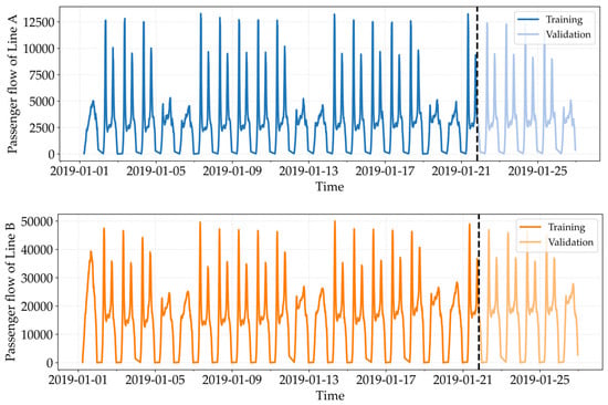
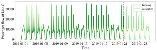
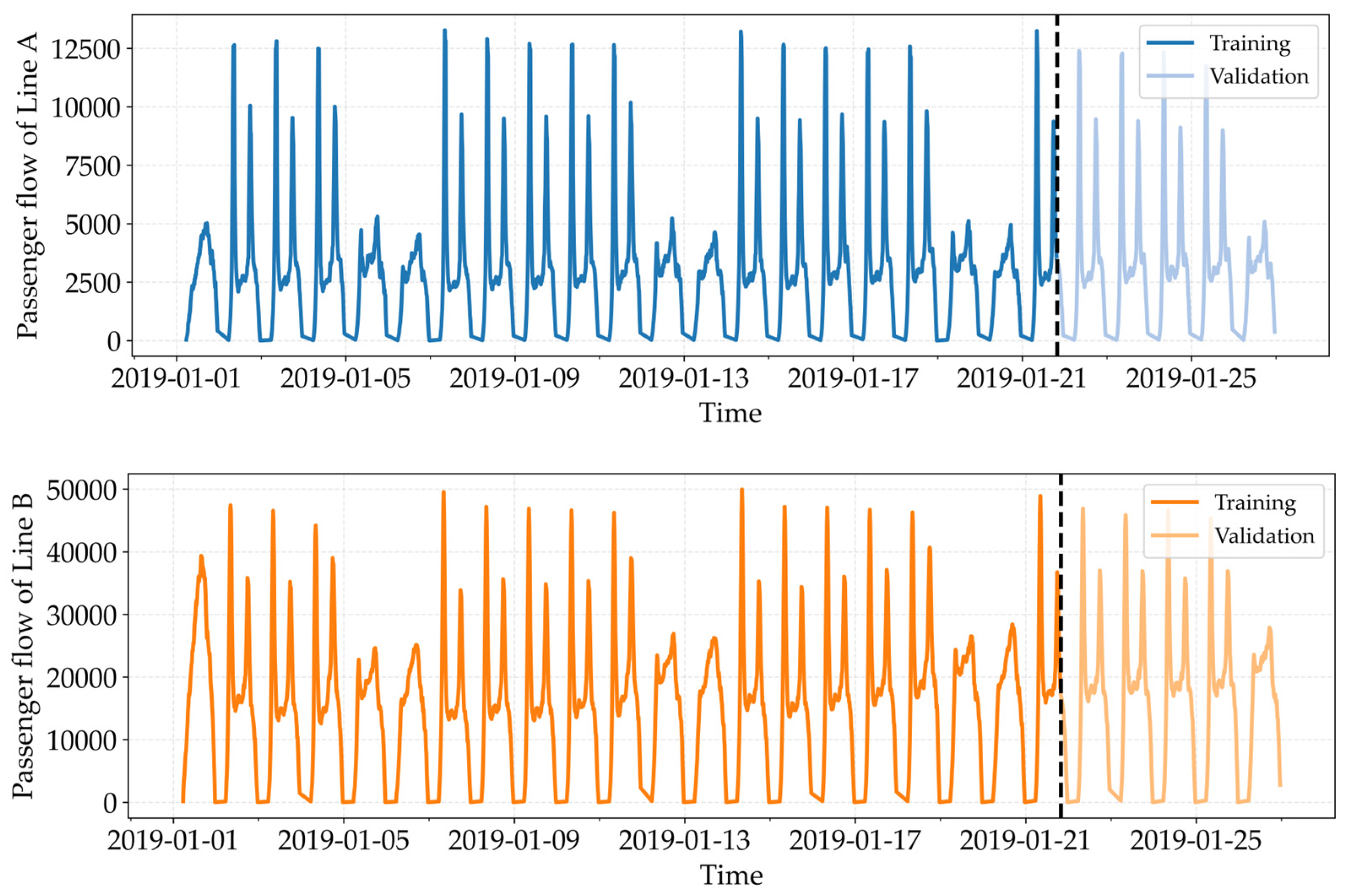
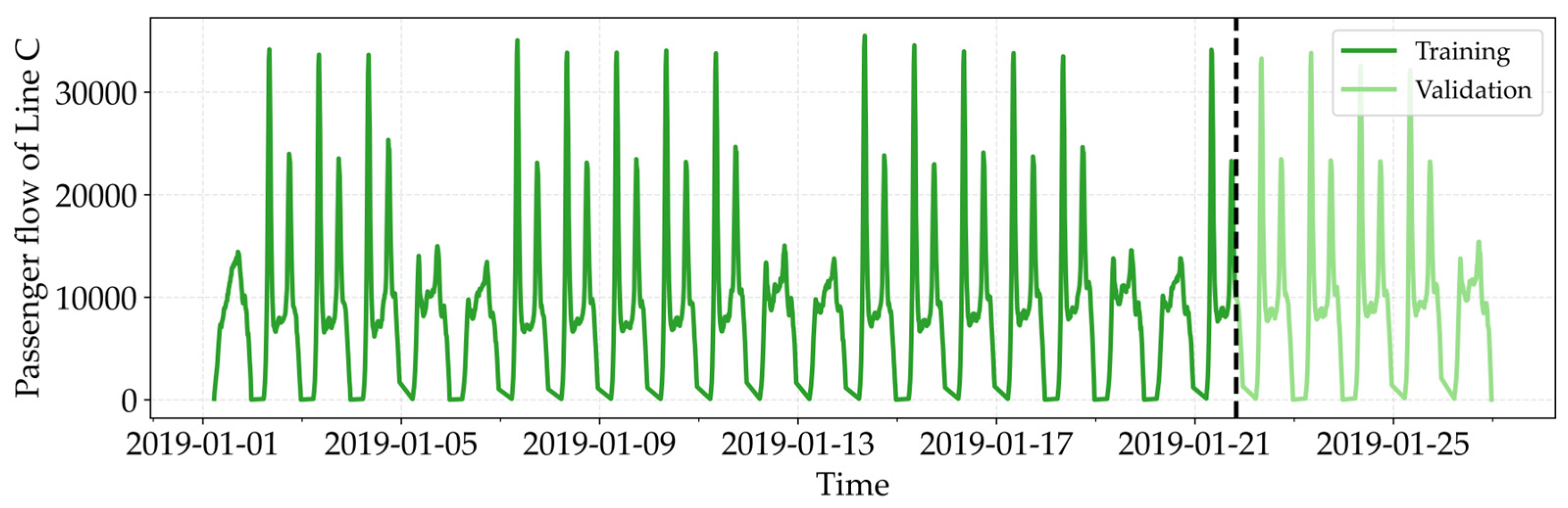
After the above processing, the station- and line-level passenger flows, recorded in 15-minute intervals, were considered as the forecasting target. The passenger flow data for Lines A, B and C are shown in Figure 6.

As shown in Figure 6, the passenger flows on Lines A, B and C all exhibited cyclical fluctuations that are associated with commuting patterns on weekdays and weekends. Such fluctuations remained consistent across the training and validation periods.

Table 1. Descriptive statistics of the 15-minute interval passenger flows on three lines.

Line	Count	Mean	Std	Min	Q1	Q2	Q3	Max
A	1875	3504.1051	2466.3154	1	2429	2963	3834	13,278
B	1892	18,433.259	9558.6105	1	14,075.25	17,632	22,656.75	49,954
C	1883	10,282.736	6423.7365	1	7315.5	9028	11,582.5	35,482

presents the statistical characteristics of urban rail transit passenger flows in Lines A, B and C using the following statistical measures: “count”, which denotes the total number of passenger flows; “mean”, which represents the average; “std”, the standard deviation, “min”, which is the minimum passenger flow; “Q1”, “Q2”, and “Q3”, which indicate passenger flows in the first, second and third quartiles, respectively; and “max”, the maximum passenger flow. All values are expressed as passenger flow (persons).

As shown in Table 1, Line B had the highest average passenger flow and the largest fluctuations, which means that it has a highly variable passenger demand. Line C had a moderate average passenger flow and variability, while Line A had the minimum average passenger flow and the smallest fluctuations. All three lines experienced periods of considerably low passenger flow and severe peak-hour congestion.

Overall, the passenger flow characteristics of the three lines are different to each other. An effective forecasting model should be able to adapt to the features of different lines; therefore, studying these three lines can demonstrate the adaptivity and generalization of our forecasting model.

5.2. Lag Length Determination

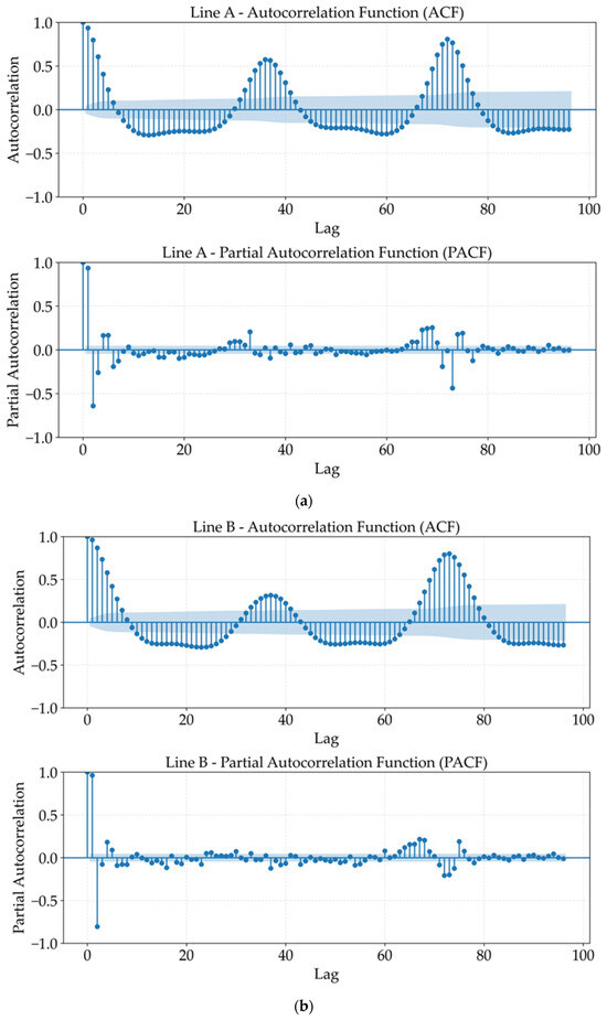
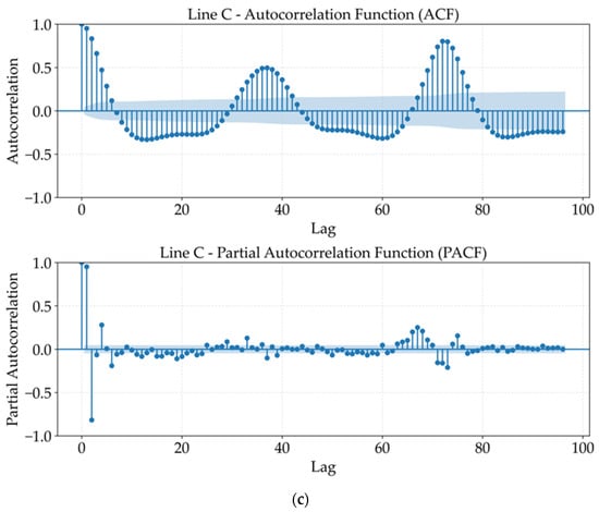
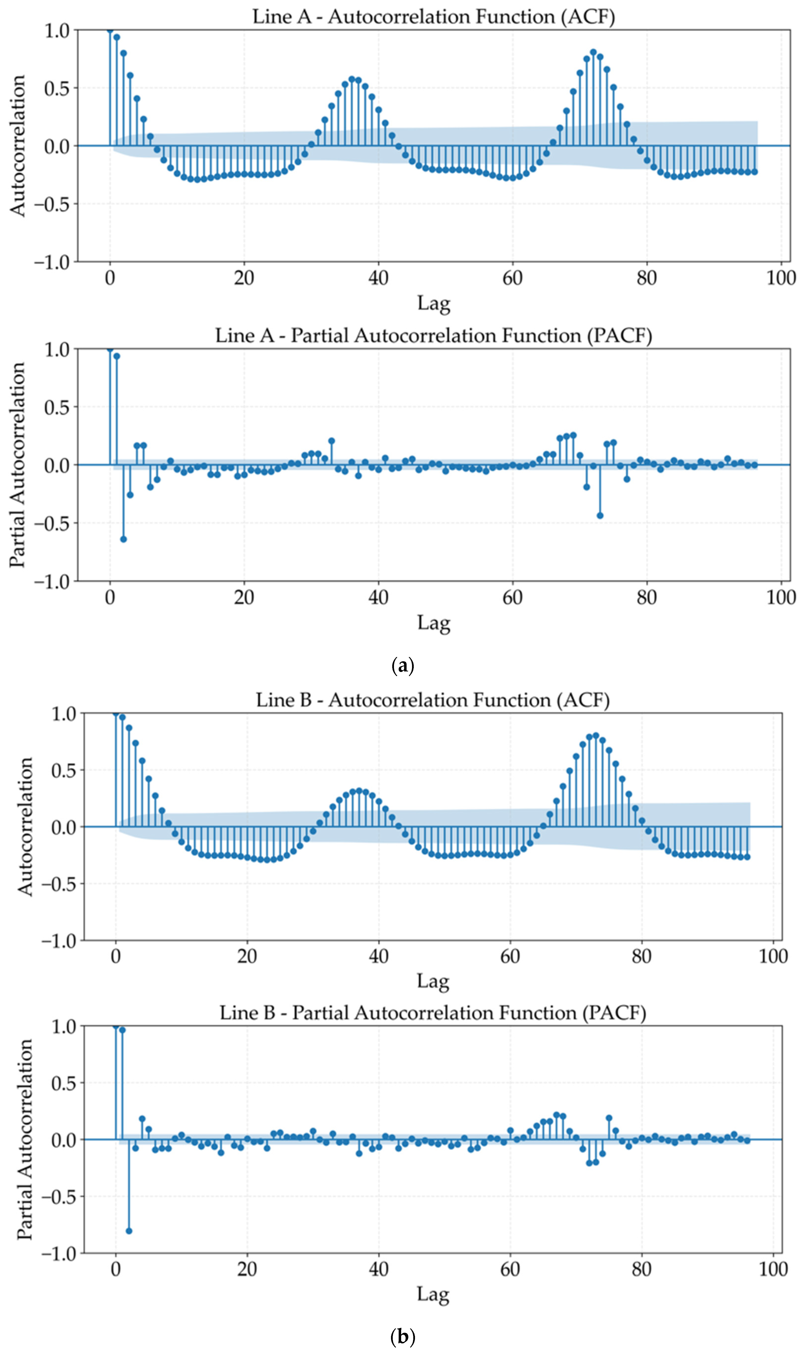
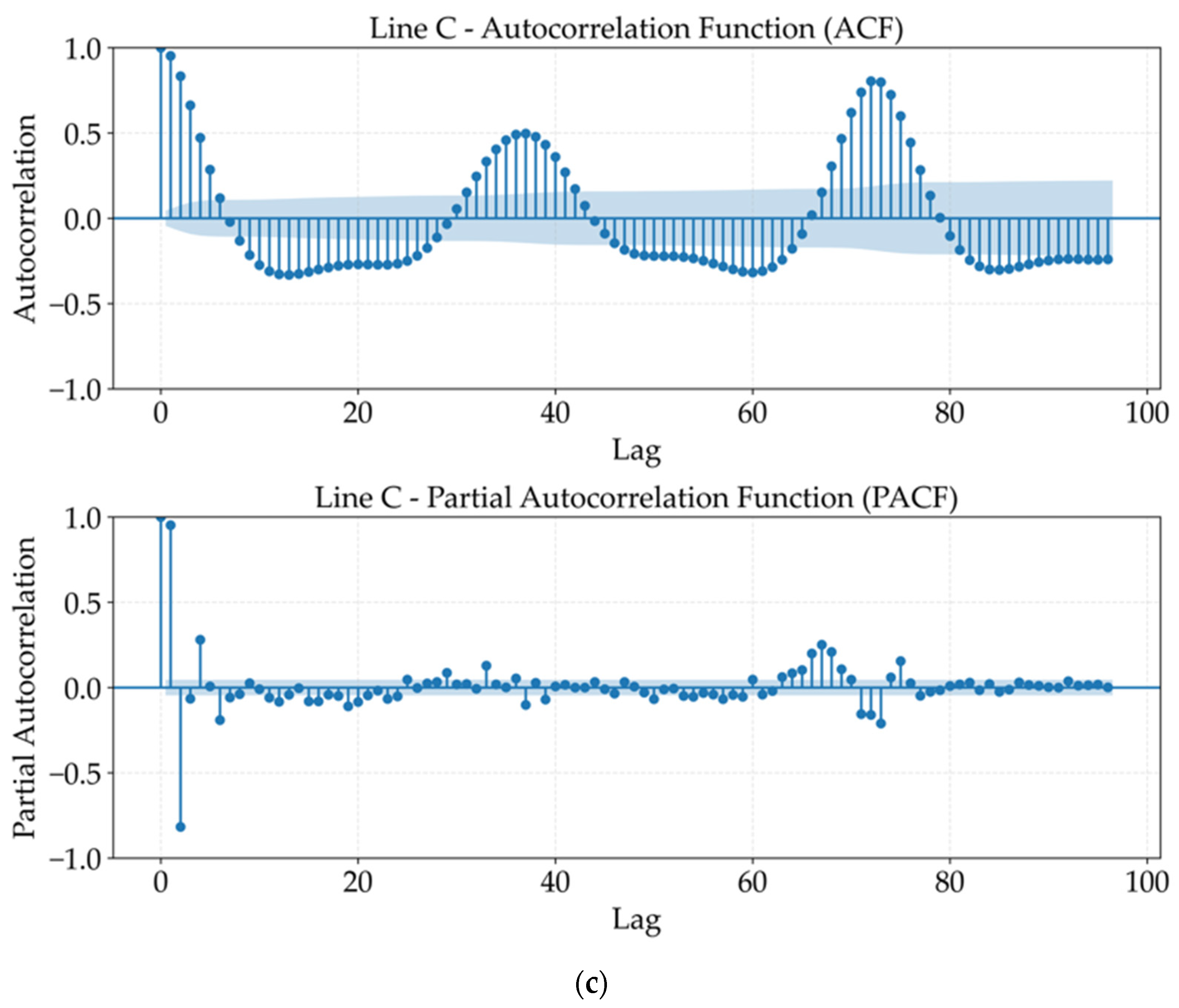
To determine an appropriate lag length $L$ for capturing short-term dependencies, we examined the temporal autocorrelation structure of the passenger flow time-series. The autocorrelation function (ACF) and partial autocorrelation function (PACF) were computed and plotted for each of the three lines. These plots provide insight into the extent to which current passenger flows are correlated with past flows, thereby guiding the selection of the lag length used in Equation (4).

The ACF and PACF of passenger flows for Lines A, B, and C are presented in Figure 7. The ACF revealed a clear diurnal pattern: there was a rapid decay within the first five lags, negative troughs at lags 6–28, and two positive peaks at lags 32–40 and 64–72, with the latter exceeding 0.6. The PACF exhibited extremely high values at lag 1, sharply dropped at lag 2, and became statistically insignificant after lag 5 for Lines A and B, while Line C showed slight significance at lag 3.

These results demonstrate two key characteristics of the data: strong short-term dependence, captured within five lags, and pronounced diurnal periodicity. Accordingly, setting $L=5$ in Equation (4) captures all significant short-term correlations, while sine–cosine encoding efficiently represents the periodic patterns. This combined design ensures comprehensive feature expression while avoiding the computational burden and feature redundancy that would result from including dozens of lag terms, thereby reducing model size and maintaining its efficiency.

5.3. Cluster Analysis

To construct spatial features, we employed a K-means cluster algorithm to classify the urban rail transit passenger flow into four categories. The resulting four clusters represent distinct passenger flow patterns that implicitly reflect different station functions, such as residential areas, commercial districts, transportation hubs, or mixed-use zones [40]. The proposed model can accordingly forecast the passenger flows by considering clusters containing unique station characteristics, which helps to improve the forecasting accuracy.

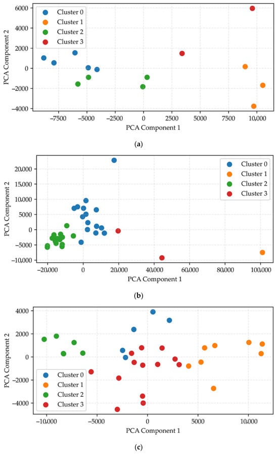
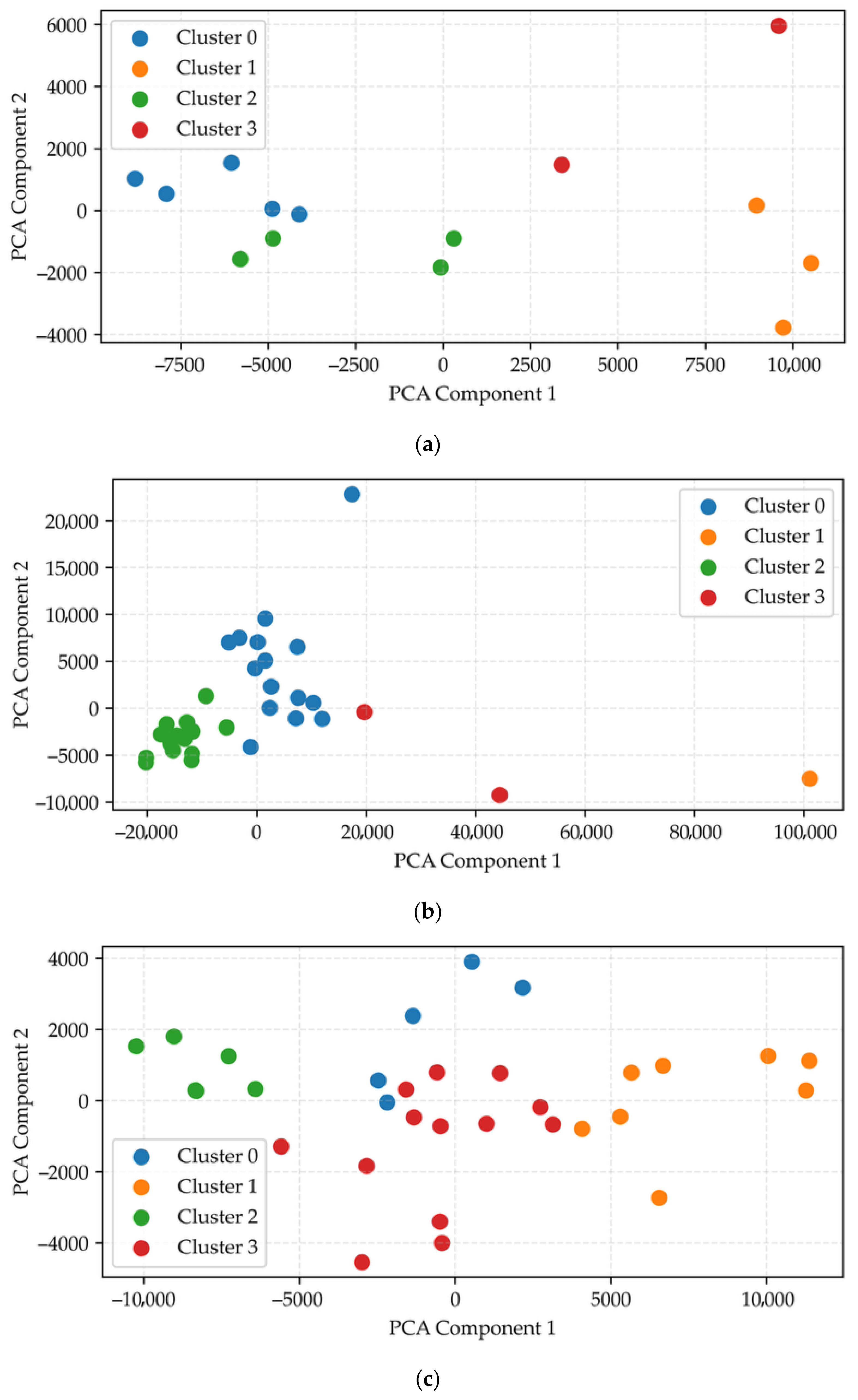
To better visualize the station clusters of the three urban rail transit lines, we reduced the original high-dimensional passenger flow features using Principal Component Analysis (PCA). All passenger flow features were projected into the first and second principal components to capture the greatest variance in the original flow data. The clustering results of the three lines are shown in Figure 8.

As illustrated in Figure 8, stations on Line A were dispersed across the plot, which reflects the substantial variation in their passenger flows. For Line B, the stations were spread widely along the first principal component, with Cluster 0 in the positive region and Cluster 2 in the negative region. This indicates a large overall difference in passenger volumes among the stations on Line B. In contrast, the stations on Line C were closely grouped together, with Clusters 0 and 3 overlapping near the origin, which suggests that passenger flows are more uniform across Line C.

Table 2. Station clusters for Lines A, B and C.

Line	Cluster 0	Cluster 1	Cluster 2	Cluster 3
A	71, 72, 74, 79, 80	76, 77, 78	67, 68, 69, 70	73, 75
B	2, 4, 5, 8, 10, 11, 12, 13, 14, 16, 18, 20, 22, 24, 33	15	0, 1, 3, 6, 17, 19, 21, 23, 25, 26, 27, 28, 29, 30, 31, 32	7, 9
C	41, 43, 44, 45, 60	46, 47, 49, 52, 53, 55, 56, 57	34, 35, 36, 40, 64, 66	37, 38, 39, 42, 48, 50, 51, 58, 59, 61, 62, 63, 65

lists the station clusters for Lines A, B and C.

The cluster labels (i.e., 0, 1, 2 and 3) of these urban rail stations were used as input (i.e., an explanatory variable) to forecast the station- and line-level passenger flows.

5.4. Comparative Experiment

5.4.1. Selected Benchmark Models for Comparative Experiments

To evaluate the proposed model, we compared it with four advanced deep learning and eight traditional machine learning benchmark models. The deep learning benchmark models, able to capture temporal dependencies, are as follows:

(1) Gated recurrent unit (GRU) with gating and lower complexity;

(2) LSTM network, which learns long-range dependencies via cell states and gates;

(3) Transformer, which uses self-attention to model the global temporal relationships;

(4) Temporal convolutional network (TCN), which applies causal and dilated convolutions to obtain a wide receptive field with clear temporal order and parallel computation.

The machine learning benchmark models are tree- and kernel-based ensemble models that exhibit strong performance on structured data. All machine learning models were trained using default parameters and are listed below:

(1) Adaptive Boosting (AdaBoost), which sequentially focuses on mispredicted samples;

(2) Categorical Boosting (CatBoost), which handles categorical features and mitigates overfitting by ordered boosting;

(3) ExtraTrees, which adds randomness to tree construction to reduce variance;

(4) Gradient Boosting Regression (GBR), which builds an additive model to minimize a differentiable loss;

(5) LightGBM, which uses efficient histogram-based and leaf-wise gradient boosting;

(6) Random forest (RF), which aggregates multiple trees trained by bootstrapped samples and random feature subsets;

(7) Support Vector Regression (SVR), which fits data within a tolerance margin via kernels in high-dimensional space;

(8) Extreme Gradient Boosting (XGBoost), which performs regularized gradient tree boosting with high speed and accuracy.

The parameter settings of all the benchmark models are listed in

Table 3. Parameter settings of the benchmark models.

Model	Parameter	Value	Model	Parameter	Value
LGBM	num leaves	31	LSTM	hidden size	128
	min child samples	20		num layers	2
	learning rate	0.1		dropout	0.2
	estimators	100		batch size	32
	max depth	10		epochs	200
XGBoost	max depth	6	GRU	hidden size	128
	learning rate	0.3		num layers	2
	n estimators	100		dropout	0.2
	gamma	0		batch size	32
	subsample	1		epochs	200
CatBoost	iterations	1000	Transformer	d model	128
	depth	6		n head	8
	learning rate	0.03		num layers	3
	l2 leaf reg	3		batch size	32
	random strength	1		epochs	200
GBR	n estimators	100	TCN	num channels	[64, 128, 256]
	learning rate	0.1		kernel size	3
	max depth	3		dropout	0.2
	min samples split	2		batch size	32
	min samples leaf	1		epochs	200
RF	n estimators	100	AdaBoost	n estimators	50
	max depth	10		learning rate	1
	min samples split	2		loss	linear
	min samples leaf	1	SVR	penalty parameter	1
	max features	sqrt		epsilon	0.1
ExtraTrees	n estimators	100		kernel	rbf
	max depth	10
	min samples split	2
	min samples leaf	1
	max features	Sqrt

; the parameter settings of the model proposed in this study are given in

Table 4. Parameter settings of the proposed model.

Model		Parameter	Value
Ensemble Learning Model	ExtraTrees	n estimators	100
		max depth	10
		min sample split	2
		min sample leaf	1
		max features	sqrt
	LGBM	num leaves	31
		min child samples	20
		learning rate	0.1
		n estimators	100
		max depth	10
	PSO	particles	10
		iterations	20
		inertia weight	0.6
		cognitive acceleration coefficient	1.4
		social acceleration coefficient	1.4
	Ridge	alpha	1
Spatio-Temporal Feature	Temporal Feature	lag length	5
	K-Means	n cluster	4
	Graph Feature	order of transfer matrix	2
	Attention Feature	window size	4

.

As shown in Table 4, the key spatio-temporal parameters were selected empirically from the data. For graph propagation, the transfer matrix order was set to 2, capturing both direct neighbors and stations two steps away. The attention window size was set to 4, corresponding to a one-hour history with 15-minute data, which captures short-term dependencies and recent fluctuations while remaining efficient. These settings allow for underlying patterns to be represented by features without overfitting or introducing unnecessary complexity.

5.4.2. Comparative Results

In this study, we evaluated model performance using the Root Mean Square Error (RMSE), Mean Absolute Error (MAE), Mean Absolute Percentage Error (MAPE), and the Coefficient of Determination (R²). The RMSE measures the deviation between the forecasted results and actual values and is sensitive to large errors, while the easily interpretable MAE represents the average absolute forecasting error and the MAPE expresses the forecasting accuracy as a percentage, which allows for a comparison across different data scales. Finally, R² is the proportion of variance explained by the model, where a value closer to 1.0 indicates a better fit.

(1) Station-level passenger flow forecasting results

The forecasting errors (i.e., RMSE, MAE, MAPE and R²) of the proposed model and the selected benchmark models for station-level passenger flows are presented in

Table 5. Station-level forecasting errors of the proposed model and the selected benchmark models.

Model	Line A				Line B				Line C
	RMSE	MAE	MAPE	R2	RMSE	MAE	MAPE	R2	RMSE	MAE	MAPE	R2
Our study	28.881	21.171	12.055	0.961	58.763	44.051	11.013	0.949	33.881	25.105	10.057	0.969
AdaBoost	42.891	33.619	31.335	0.930	79.011	62.823	24.934	0.918	46.640	36.933	22.676	0.944
CatBoost	32.976	23.634	12.491	0.957	60.150	45.414	11.877	0.950	36.171	26.932	11.124	0.966
ExtraTrees	32.650	23.099	12.205	0.958	60.709	45.795	11.814	0.948	35.169	26.216	10.669	0.967
GBR	35.771	25.553	13.288	0.952	65.247	49.094	13.062	0.942	38.513	28.565	11.532	0.961
GRU	34.589	25.102	13.033	0.950	65.328	49.733	11.634	0.939	37.309	28.353	11.324	0.961
LGBM	35.041	24.615	12.986	0.952	64.237	47.898	12.637	0.944	38.404	28.124	11.369	0.962
LSTM	35.672	25.766	12.999	0.947	67.659	51.502	11.950	0.935	38.218	28.925	11.494	0.959
RF	34.938	24.303	13.041	0.954	66.497	49.509	13.050	0.941	38.816	28.338	11.451	0.961
SVR	34.205	24.146	13.393	0.956	61.179	46.439	12.563	0.948	35.686	26.803	11.298	0.966
TCN	34.212	25.277	13.427	0.950	68.248	52.025	12.761	0.934	38.329	29.389	12.320	0.959
Transformer	35.453	25.377	12.671	0.945	65.477	49.709	12.021	0.932	38.089	28.796	11.420	0.958
XGBoost	37.435	25.940	13.844	0.947	68.774	51.050	13.654	0.938	40.743	29.832	12.130	0.957

. It should be noted that Table 5 presents the average forecasting errors of all stations on a line.

According to Table 5, the proposed model achieved the minimum RSME, MAE and MAPE in all cases. It also yielded the maximum R² for Lines A and C and a near-maximum R² for Line B. Therefore, we can conclude that the proposed model exhibited the best forecasting performance on all three lines compared to the benchmark models.

It should also be noted that there were much larger forecasting errors for Line B than Lines A and C across all models, since this line is a major corridor with higher passenger flow (see Table 1) and contains large transfer hubs. However, the proposed model still achieved the minimum RMSE, MAE and MAPE, which demonstrates that it is able to deal with considerable passenger flows through urban rail transit stations and thus shows high adaptivity.

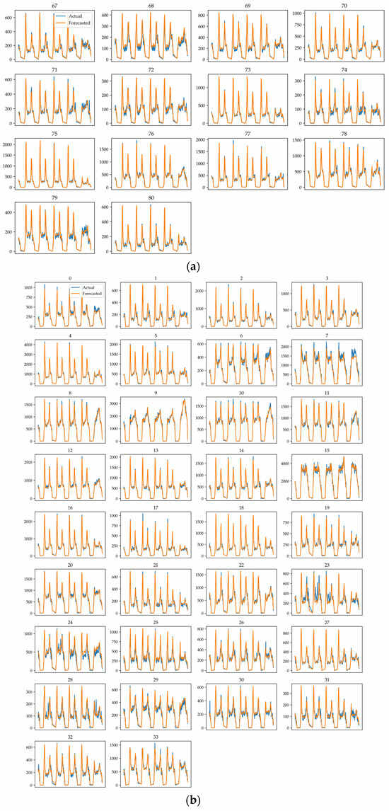
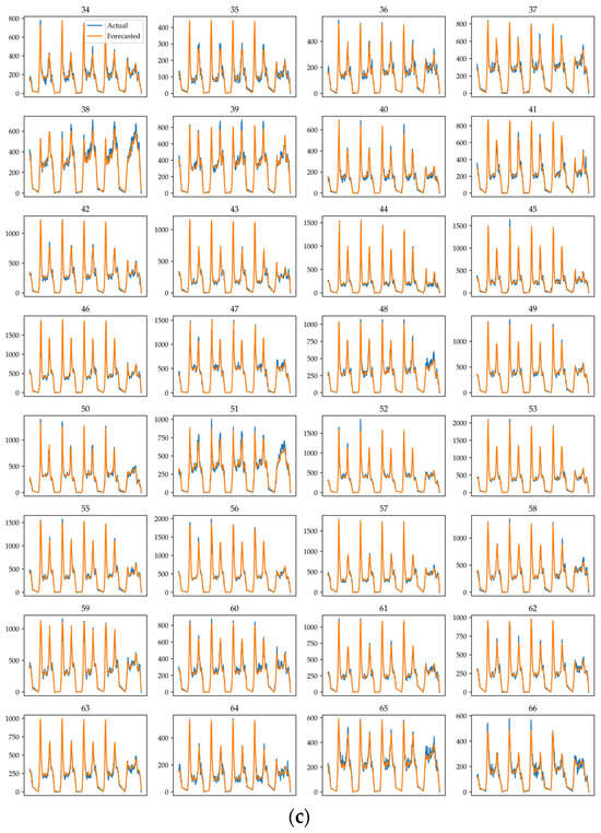
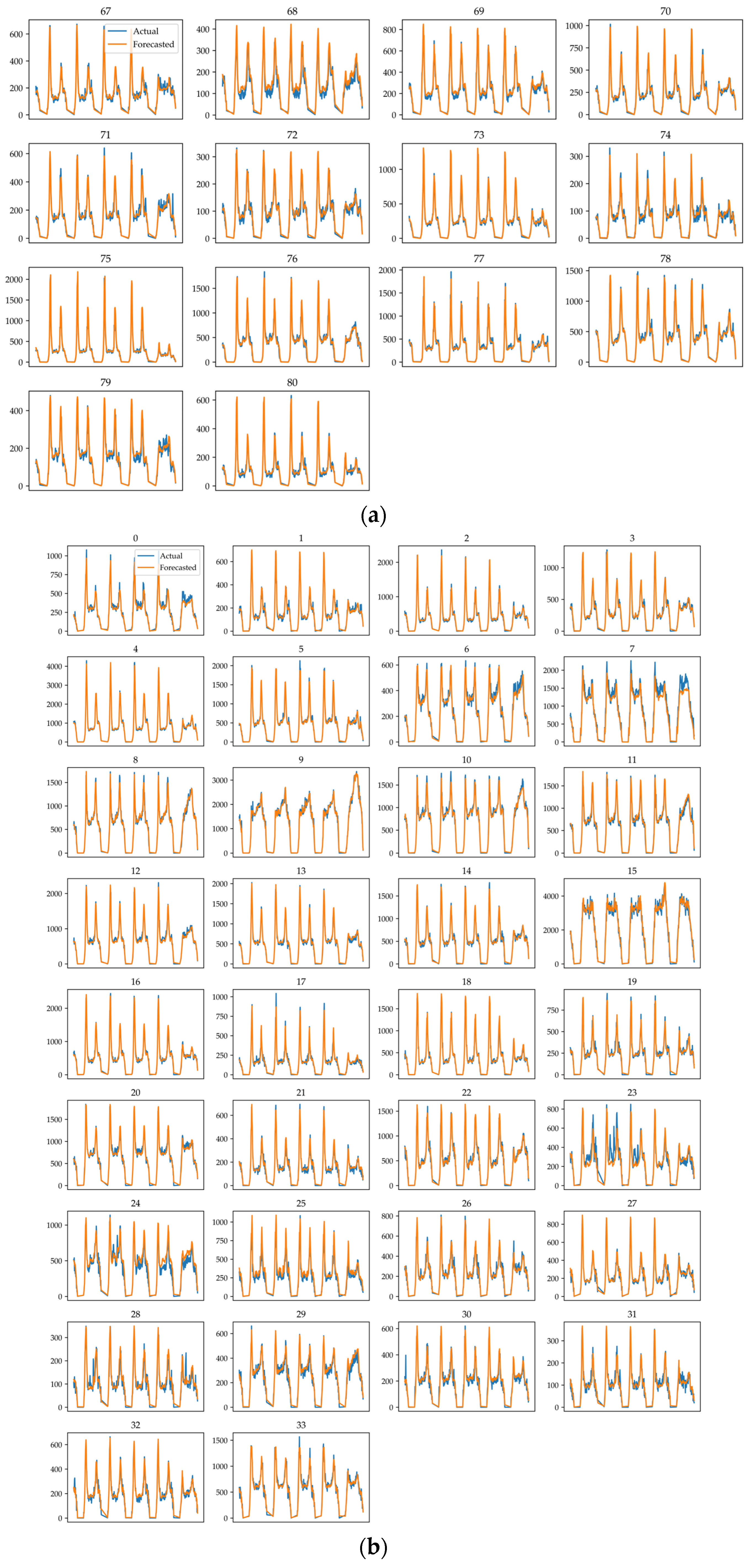
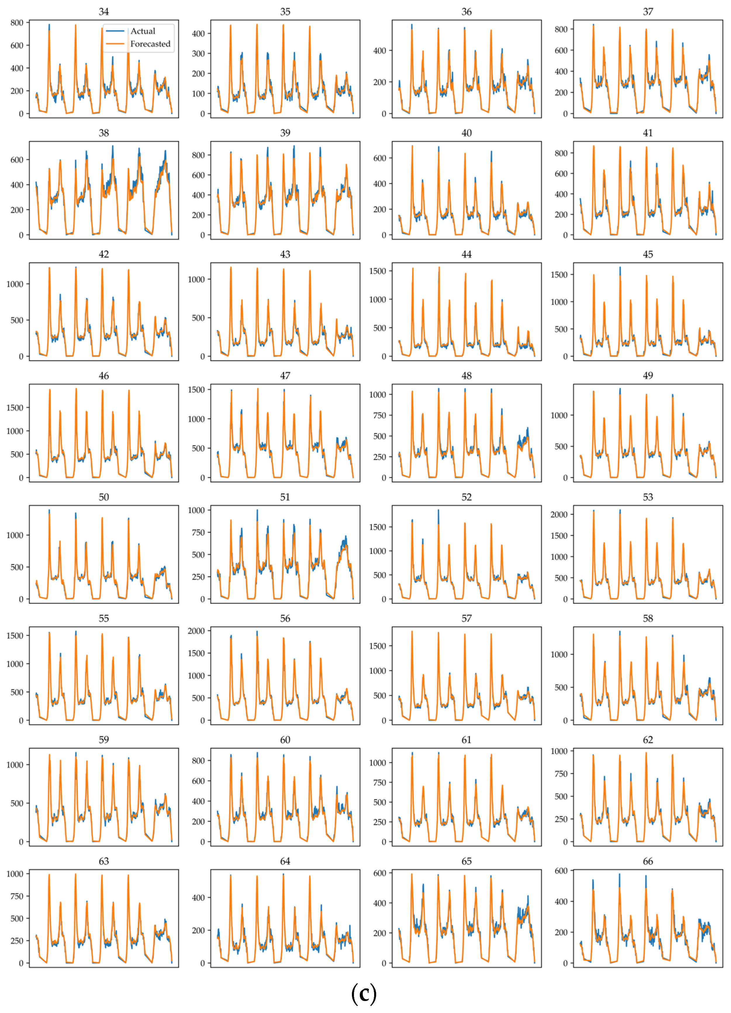
Figure 9 comprehensively illustrates the capability of the proposed model in capturing the change in passenger flows at all studied stations on Lines A, B, and C.

For the stations on Line A, passenger flows showed clear daily rises and falls with distinct peak hours, which reflect typical commuter cycles. Stations 67, 71, 75–78 particularly exhibited relatively high passenger flows during some peak hours, while the passenger flows of Stations 70 and 74 remained lower and steadier. According to Figure 9a, the proposed method can effectively capture the temporal correlations and daily cycles in the passenger flow data for all stations on Line A.

For the stations on Line B, passenger flows varied greatly. These stations include not only high-volume transfer hubs with severe crowding (e.g., Station 15) but also small-scale stations with lower passenger demand (e.g., Station 31). The spatial links between the stations in Line B are thus complicated. However, based on Figure 9b, the proposed model still successfully learnt the above characteristics in passenger flows for all stations on Line B.

For the stations on Line C, passenger flows were more regular and stable compared to Lines A and B. Daily commute trends were consistent across stations on Line C, which exhibited similar peak hours and less variation. Moreover, Line C had more uniform passenger flows, which makes station-level forecasting easier. As indicated by Figure 9c, the proposed model can accurately match the above regularity, stability and consistency.

Overall, the proposed model can accurately capture the variations in station-level passenger flows in both regular and peak periods, and exhibits accurate forecasting for urban rail transit stations with different passenger flow characteristics.

(2) Line-level passenger flow forecasting results

The line-level passenger flow forecasts for the benchmark models were obtained by summing the forecasted results (from the same model) of all stations on the line. In contrast, the proposed model used meta-learning to optimize the forecasts of both station- and line-level passenger flows. The line-level passenger flow forecasting errors of the proposed model and benchmark models are presented in

Table 6. Line-level passenger flow forecasting errors of the proposed model and benchmark models.

Model	Line A				Line B				Line C
	RMSE	MAE	MAPE	R2	RMSE	MAE	MAPE	R2	RMSE	MAE	MAPE	R2
Our study	149.53	109.43	4.06	0.996	523.84	402.12	2.80	0.997	310.54	227.60	2.78	0.998
AdaBoost	351.45	258.82	62.41	0.979	1257.34	967.69	27.82	0.982	735.43	607.13	34.98	0.987
CatBoost	233.68	154.59	8.89	0.991	668.47	493.42	4.53	0.995	426.29	315.03	8.73	0.996
ExtraTrees	228.87	143.36	7.41	0.991	681.37	508.89	4.31	0.995	407.20	301.33	7.23	0.996
GBR	213.24	171.07	12.98	0.992	1119.80	926.04	8.25	0.984	535.90	409.67	7.64	0.993
GRU	219.02	147.95	11.85	0.991	796.08	600.37	4.76	0.992	461.95	349.52	11.51	0.994
LGBM	225.55	149.80	9.56	0.991	667.83	515.30	5.05	0.995	394.11	291.04	7.54	0.996
LSTM	239.44	158.88	12.23	0.990	869.54	650.21	5.33	0.991	509.56	380.52	11.89	0.993
RF	244.52	153.23	9.88	0.990	769.74	578.26	5.49	0.993	428.71	315.18	9.27	0.996
SVR	264.02	162.48	12.35	0.988	733.05	571.06	6.26	0.994	483.47	369.06	10.98	0.994
TCN	201.94	138.69	12.73	0.993	902.80	684.20	7.13	0.990	464.84	357.46	13.19	0.994
Transformer	222.27	142.25	9.73	0.991	739.01	570.61	5.18	0.993	411.48	306.11	8.34	0.996
XGBoost	252.81	157.55	7.67	0.989	712.17	547.71	5.64	0.994	430.15	317.47	7.18	0.995

.

As shown in Table 6, the proposed model achieved the best performance in forecasting line-level passenger flows compared to the benchmark models, yielding the minimum RMSE, MAE and MAPE and maximum R² for all three lines. Thus, the combination of multi-source spatio-temporal features and optimized ensemble learning is effective in forecasting the line-level passenger flows of urban rail transit systems.

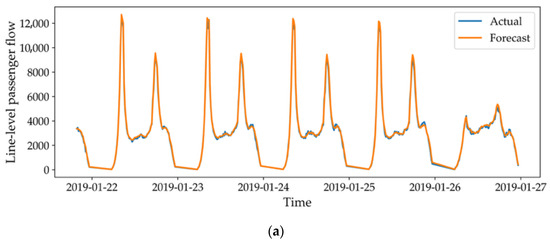
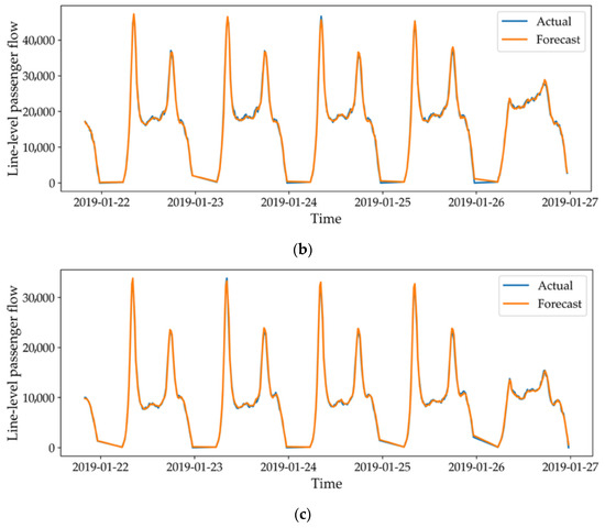
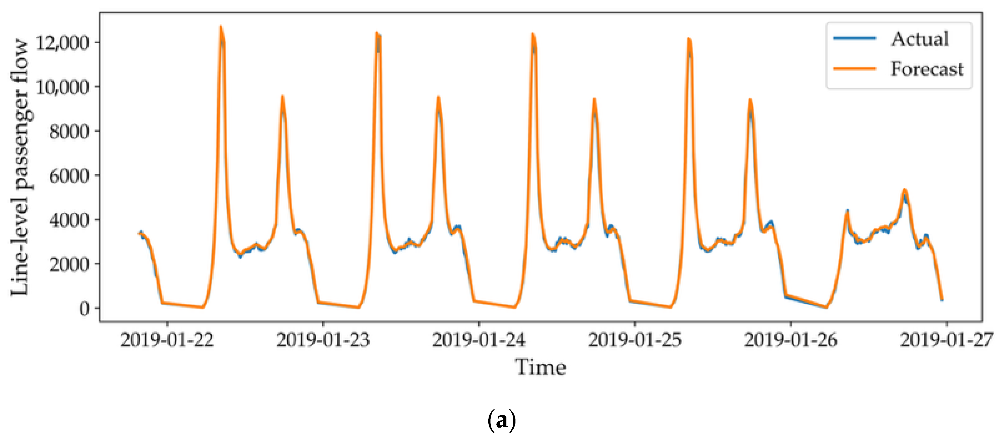
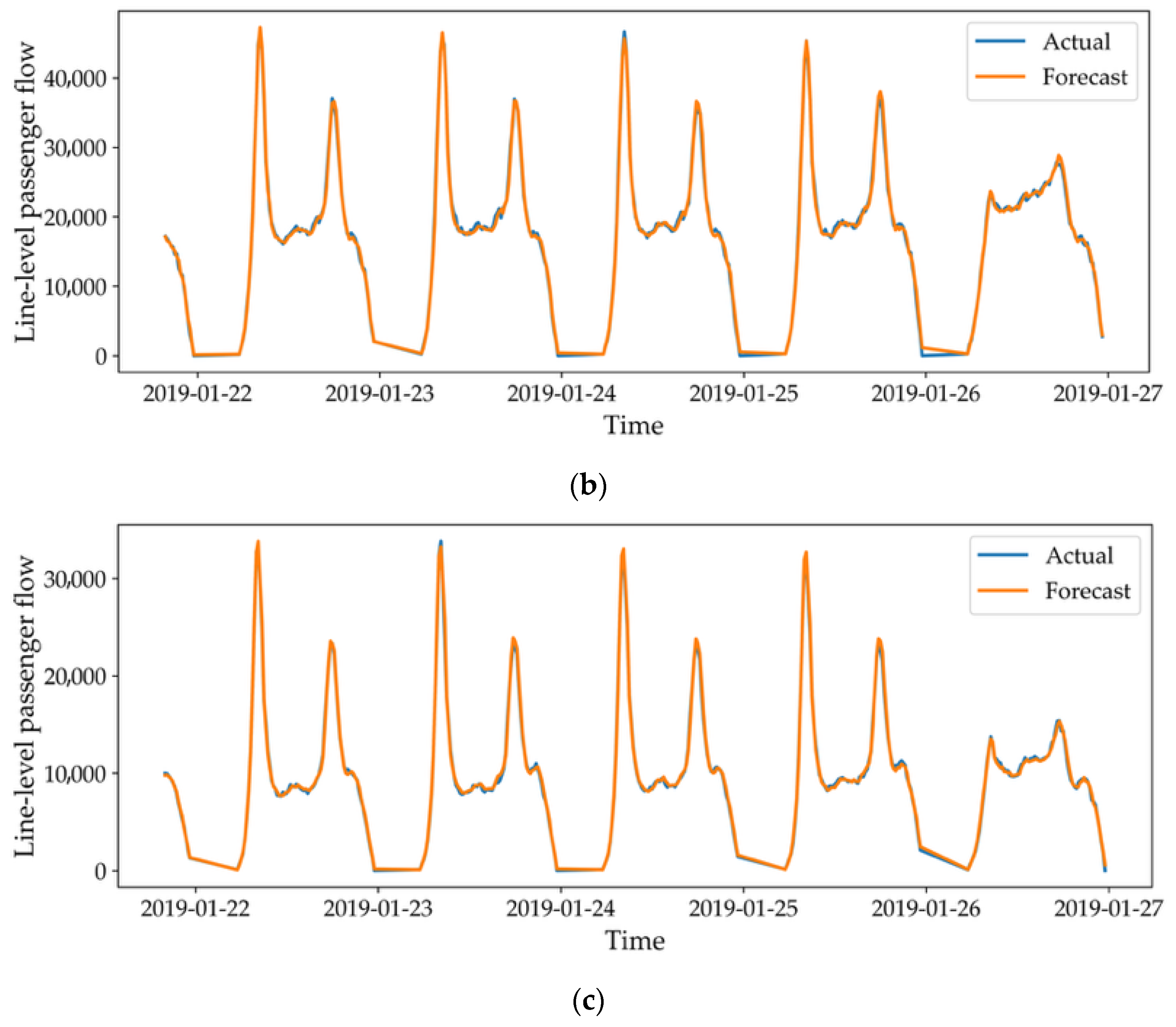
Figure 10 visually illustrates the performance of the proposed model in line-level passenger flow forecasting.

The passenger flow of Line A was the lowest among the three lines, exhibiting moderate peak hours and clear drops in passenger flow on weekends. Additionally, passenger volumes differed greatly between weekdays and weekends, and weekly changes were gentler during off-peak hours. As illustrated in Figure 10a, the proposed model is a suitable choice for urban rail transit lines with the above characteristics.

For Line B, passenger flow was the highest, and there was severe overcrowding during the morning and evening peak hours and large decreases during the off-peak hours. Its passenger flows and intensity were considerably greater than those of Line A. However, according to Figure 10b, the proposed model could still handle this situation well.

For Line C, passenger flow and variation were intermediate compared to Lines A and B. Figure 10c demonstrates that the proposed model still effectively handled these features to achieve an accurate forecast.

Above all, the close alignment between the actual and forecasted curves for all three lines demonstrates the ability of the proposed model to capture the overall temporal dynamics of and fluctuations in line-level passenger flows for urban rail transit lines with varying passenger flow characteristics.

The results indicate that meta-learning based on ridge regression can effectively optimize and balance station- and line-level passenger flow forecasts to achieve consistency between them. The proposed model is effective in forecasting these flows across both levels, and exhibits high adaptivity and generalizability to handle stations and lines with different passenger flow characteristics.

5.5. Performance Analysis on Station Clustering

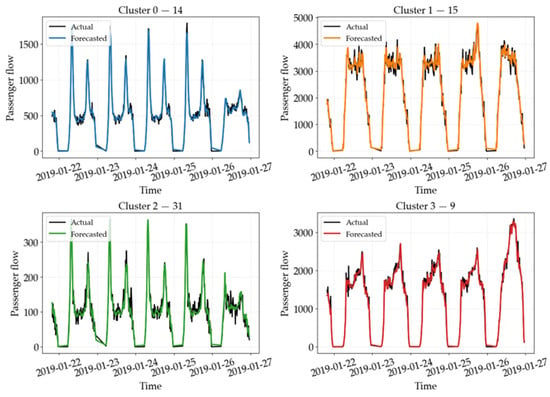
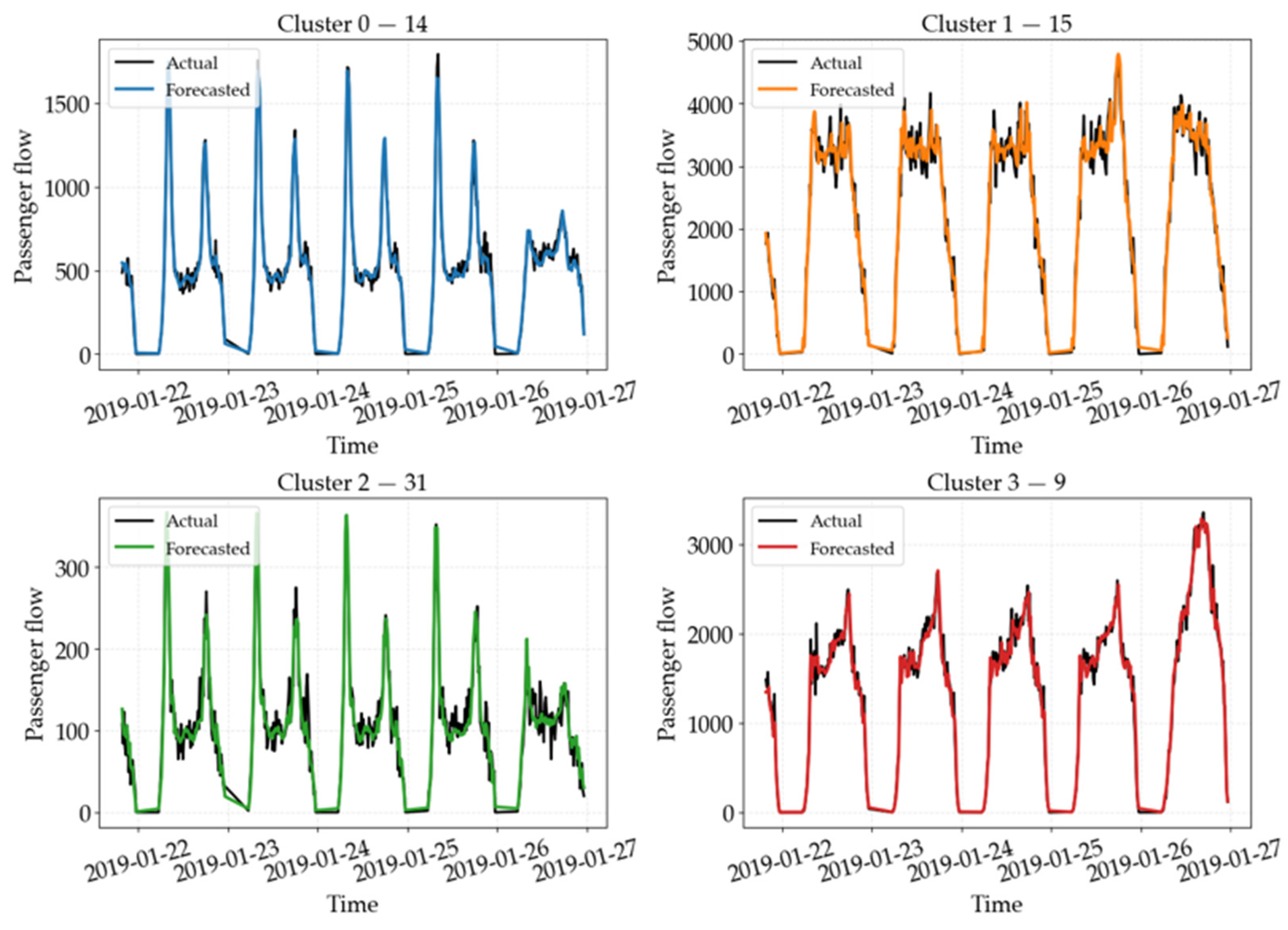
To further investigate the forecasting performance across different station types, we analyzed the station clustering results on Line B. As described in Section 5.2, the stations on Line B were grouped into four clusters based on their passenger flow patterns. For each cluster, we selected the station with the lowest RMSE as a representative and plotted its actual versus forecasted passenger flows over the test period, as shown in Figure 11.

As shown in Figure 11, cluster 0 contained 14 stations typical of residential or peripheral areas, with sharp morning peaks of above 1600 passengers, near-zero overnight flows, and rapid evening declines. The model closely tracked the steep morning rise and evening drop, matching the commute-driven demand profile. Even when volumes were near zero in early morning hours, forecasts remained tightly aligned with the observations, indicating that the model effectively learns station-specific diurnal rhythms.

Cluster 1 included 15 stations functioning as high-volume central business district nodes or major transfer hubs. Their passenger flow profiles featured sustained loads ranging from 3000 to 4500 passengers throughout the day, with flattened peak structures that lacked the sharp spikes seen in residential stations. The model achieved strong alignment during both morning and evening peak periods, and maintained reasonable accuracy during off-peak hours. This consistent performance reflects the stable, high-density demand characteristic of commercial centers, where passenger activity remains elevated across a broad daytime window rather than concentrating into narrow peaks.

Cluster 2, the largest group with 31 stations, displayed moderate-volume mixed-use patterns. These stations exhibited irregular peak structures and higher intraday volatility compared to the other clusters, indicative of diverse trip purposes, including commuting, shopping, and leisure activities. Despite this complexity, the model successfully followed the overarching trend and captured the principal fluctuations throughout each day. The forecasts adapted well to the variable demand patterns, underscoring the model’s robustness when faced with heterogeneous station functions.

Cluster 3 contained nine stations with evening-dominated patterns typical of entertainment districts or commercial areas oriented toward nighttime activity. Passenger flow gradually ascended during the afternoon and accelerated through the early evening, culminating in pronounced late-evening peaks exceeding 3000 passengers. The model accurately reproduced this distinctive temporal shift, tracking the evening surge with precision and maintaining fidelity throughout the extended active period.

In summary, the model fit morning commute clusters tightly and performed best during the peak period for evening entertainment clusters. The off-peak daytime accuracy stayed high in business districts, and the model exhibited low deep off-peak absolute errors, aligned with reduced demand. These results have direct operational implications: reliable peak forecasts can be used in high-volume hubs for dynamic headway adjustments; in residential stations to optimize early-morning deployment; in mixed-use areas to integrate real-time data; and in evening-centric stations to justify increased late-night train frequencies.

6. Conclusions

This study addressed the problem of forecasting passenger flow in urban rail transit at the station and line levels, and a novel forecasting model was proposed that integrates multi-source spatio-temporal features and optimized ensemble learning. The main contributions of this study are as follows:

(1) A comprehensive multi-source spatio-temporal feature engineering framework was proposed to effectively capture the complex and nonlinear dynamics of station-level passenger flow. It systematically extracts and fuses different features, including temporal periodic features, lag features, and spatial features derived from graph adjacency; an attention mechanism; and station clustering.

(2) A dynamically weighted ensemble forecasting framework was developed to enhance robustness and accuracy. It employs ExtraTrees and LightGBM as base models and utilizes the PSO algorithm to adaptively determine their optimal combination weights based on optimizations of the validation performance.

(3) A meta-learning-based collaborative forecasting mechanism was introduced to optimize and balance station- and line-level forecasts. Ridge regression was used as the meta-learner and trained to process station-level forecasts in order to obtain line-level forecasts.

(4) A systematic validation experiment based on passenger flow data from three urban rail transit lines in Hangzhou was conducted to verify the advantages of the proposed model. Through comparative experiments, it was verified that the proposed model yields higher accuracy and robustness and is more applicable to real situations.

The results of this study show that the proposed model can provide solid decision support for operations, management, and planning departments across stations and the entire network, including support for real-time crowd management, dynamic train scheduling, and efficient resource allocation.

However, the proposed model still has the following limitations that should be addressed in future research.

(1) The proposed model relies on passenger flow data extracted from smart card transactions and does not incorporate external geospatial information. Due to the nature of the public dataset, the specific physical alignments of the three lines were not explicitly defined, preventing us from inferring the precise geographical locations of stations and their surrounding land use characteristics. Consequently, important exogenous factors such as points of interest, employment density, and residential distribution—which significantly influence passenger demand—could not be integrated into the feature engineering stage.

(2) The proposed model groups stations using clustering based solely on passenger flow time-series, without considering functional classifications such as transfer hub, commercial center, or residential area. The lack of ground-truth station function labels, again attributable to the absence of external data sources, limits our ability to validate whether the identified clusters truly reflect operational roles within the network.

(3) The proposed model was validated using a public dataset containing data across a single month (January 2019), which may not fully capture seasonal variations, holiday effects, or long-term ridership trends. No additional data from different seasons or years were available to assess the model’s robustness under varying temporal conditions.

To address the above limitations, future research will be conducted in the following directions.

(1) To address the lack of external geospatial information, we will integrate smart card data with multi-source geospatial datasets, including POIs, land use maps, and demographic statistics. Using spatial analysis methods such as geographically weighted regression or graph neural networks with external node features, we will quantify how urban forms and land use affect passenger flows, improving the model’s explanatory power and accuracy.

(2) In future work, we will refine station clustering by adding functional classification variables from external data, including POI data, transfer station attributes, and employment density. We will develop hybrid clustering methods that combine passenger flow time-series with these indicators to better represent stations’ operational roles and enhance the interpretability of cluster-based features.

(3) We will strengthen the model’s robustness by validating it on longer-term datasets covering multiple seasons and years, enabling the analysis of seasonal fluctuations, holiday effects, and long-term ridership trends. We will also incorporate time-varying external factors, such as weather and special events, into the feature engineering stage so that the model can capture more complex temporal dynamics and be more useful in practice.

References

- Yang, Y.; Zhu, J.; Zhang, C.; Yang, X. Traffic Congestion Source Back-Tracing Framework for Urban Road Networks Using Traffic Volume Data. Transp. Res. Rec. 2026, 2680, 182–203. [Google Scholar] [CrossRef] [Scilit]
- Wang, L.; Jin, J.G. Utilizing and optimizing non-disrupted lines for evacuating passengers in Urban rail transit networks during disruptions. Transp. B Transp. Dyn. 2025, 13, 2440588. [Google Scholar] [CrossRef] [Scilit]
- Wang, Z.; Zheng, X.; Meng, F.; Wang, K.; Wu, X.; Yu, D. Exploring the joint influence of built environment factors on urban rail transit peak-hour ridership using DeepSeek. Buildings 2025, 15, 1744. [Google Scholar] [CrossRef] [Scilit]
- Li, C.X.; Yoon, C.J. Analysis of urban rail public transport space congestion using graph fourier transform theory: A focus on Seoul. Sustainability 2025, 17, 598. [Google Scholar] [CrossRef] [Scilit]
- Chuwang, D.D.; Chen, W.; Zhong, M. Short-term urban rail transit passenger flow forecasting based on fusion model methods using univariate time series. Appl. Soft Comput. 2023, 147, 110740. [Google Scholar] [CrossRef] [Scilit]
- Xiu, C.; Sun, Y.; Peng, Q. Modelling traffic as multi-graph signals: Using domain knowledge to enhance the network-level passenger flow prediction in metro systems. J. Rail Transp. Plan. Manag. 2022, 24, 100342. [Google Scholar] [CrossRef] [Scilit]
- Liu, F. A passenger flow prediction method using SAE-GCN-BiLSTM for Urban Rail Transit. Int. J. Swarm Intell. Res. 2024, 15, 1–21. [Google Scholar] [CrossRef] [Scilit]
- Huang, H.; Mao, J.; Lu, W.; Hu, G.; Liu, L. DEASeq2Seq: An attention based sequence to sequence model for short-term metro passenger flow prediction within decomposition-ensemble strategy. Transp. Res. Part C Emerg. Technol. 2023, 146, 103965. [Google Scholar] [CrossRef] [Scilit]
- Li, D.; Du, S.; Hou, Y. Long-term passenger flow forecasting for rail transit based on complex networks and informer. Sensors 2024, 24, 6894. [Google Scholar] [CrossRef] [Scilit]
- Ayub, S.; Hou, Y. Impact of the built environment on urban mobility patterns and advanced transport dynamics: A systematic review. Transp. Res. Interdiscip. Perspect. 2026, 36, 101842. [Google Scholar] [CrossRef] [Scilit]
- Liu, Y.; Du, H. The built environment and urban vibrancy: A data-driven study of non-commuters’ destination choices around metro stations. Land 2025, 14, 1619. [Google Scholar] [CrossRef] [Scilit]
- Zhou, Y.; Li, L.; Zhang, Y. Location of transit-oriented development stations based on multimodal network equilibrium: Bi-level programming and paradoxes. Transp. Res. Part A Policy Pract. 2023, 174, 103729. [Google Scholar] [CrossRef] [Scilit]
- Dindar, S. A Systematic Review of Urban Regeneration’s Impact on Sustainable Transport: Traffic Dynamics, Policy Responses, and Environmental Implications. Sustain. Dev. 2025, 33, 399–426. [Google Scholar] [CrossRef] [Scilit]
- Wang, J.; Liu, C.; Wu, Z.; Liao, R.; Li, G.; Lu, H. The roadmap and strategy for prioritizing the development of public transport in China. Multimodal Transp. 2025, 4, 100184. [Google Scholar] [CrossRef] [Scilit]
- Gao, C.; Lai, X.; Li, S.; Cui, Z.; Long, Z. Bibliometric insights into the implications of urban built environment on travel behavior. ISPRS Int. J. Geo-Inf. 2023, 12, 453. [Google Scholar] [CrossRef] [Scilit]
- Shi, Z.; Liu, X.; Qian, Q.; He, M.; Liu, Y. Research on the influence mechanism of passenger flow in urban rail transit network based on panel data analysis. Urban Rapid Rail Transit 2025, 38, 46–52. [Google Scholar]
- Beza, A.D.; Saidi, S.; Demissie, M.G.; Kattan, L. Optimizing station placement for integrated shared micromobility and public transit networks. In 2024 IEEE 27th International Conference on Intelligent Transportation Systems (ITSC), Edmonton, AB, Canada, 24–27 September 2024; IEEE: New York, NY, USA, 2024; pp. 4138–4144. [Google Scholar]
- Yuan, H.; Xu, D.; Gong, L.; Hui, C.; Geng, H.; Zhong, M. A review of passenger flow allocation methods in urban rail transit. Railw. Transp. Econ. 2025, 47, 1–17. [Google Scholar] [CrossRef]
- Zhang, P.; Li, Z.; Zhang, X.; Wang, Y. Spatiotemporal heterogeneity and nonlinear analysis of factors influencing rail transit ridership: A case study of Tianjin urban rail transit. Urban Rapid Rail Transit 2025, 38, 22–30. [Google Scholar]
- Cui, M.; Yu, L.; Nie, S.; Dai, Z.; Ge, Y.E.; Levinson, D. How do access and spatial dependency shape metro passenger flows. J. Transp. Geogr. 2025, 123, 104069. [Google Scholar] [CrossRef] [Scilit]
- Xue, Q.; Cheng, L.; Li, Z.; Xing, Y.; Wang, H.; Li, H.; Peng, Y. Unraveling spatial–temporal and interactive impact of built environment on metro ridership: A case study in Shanghai, China. Sustainability 2025, 17, 9479. [Google Scholar] [CrossRef] [Scilit]
- Zhao, X.; Li, Y.; Sun, J.; Li, L.; Ren, G. The influences of built environment on ultra-peak for urban rail transit station passenger flows based on lasso-multiscale geographically weighted regression. Travel Behav. Soc. 2025, 41, 101063. [Google Scholar] [CrossRef] [Scilit]
- Liu, S.; Rong, J.; Zhou, C.; Gao, Y.; Xing, L. Temporal Heterogeneity in Land Use Effects on Urban Rail Transit Ridership—Case of Beijing, China. Land 2025, 14, 665. [Google Scholar] [CrossRef] [Scilit]
- Zhang, P.; Li, Z.; Zhang, X.; Yue, X. Spatiotemporal influence mechanisms of urban rail transit passenger flow in different time periods. J. Transp. Syst. Eng. Inf. Technol. 2025, 25, 24–33. [Google Scholar]
- Zhang, G.; Jin, H. Research on short-term passenger flow forecast for urban rail transit based on improved ARIMA model. Comput. Appl. Softw. 2022, 39, 339–344. [Google Scholar]
- Li, J.; Peng, Q.; Yang, Y. Passenger flow prediction for Guangzhou-Zhuhai intercity railway based on SARIMA model. J. Southwest Jiaotong Univ. 2020, 55, 41–51. [Google Scholar]
- Liang, S.; Ma, M.; He, S.; Zhang, H. Short-term passenger flow prediction in urban public transport: Kalman filtering combined k-nearest neighbor approach. IEEE Access 2019, 7, 120937–120949. [Google Scholar] [CrossRef] [Scilit]
- Song, Y.; Duan, H.; Cheng, Y. A novel fractional-order grey Euler prediction model and its application in short-term traffic flow. Chaos Solitons Fractals 2024, 189, 115722. [Google Scholar] [CrossRef] [Scilit]
- Zhang, J.; Mao, S.; Zhang, S.; Yin, J.; Yang, L.; Gao, Z. EF-former for short-term passenger flow prediction during large-scale events in urban rail transit systems. Inf. Fusion 2025, 117, 102916. [Google Scholar] [CrossRef] [Scilit]
- Sun, Y.; Leng, B.; Guan, W. A novel wavelet-SVM short-time passenger flow prediction in Beijing subway system. Neurocomputing 2015, 166, 109–121. [Google Scholar] [CrossRef] [Scilit]
- Yu, J.; Chang, X.; Hu, S.; Yin, H.; Wu, J. Combining travel behavior in metro passenger flow prediction: A smart explainable Stacking-CatBoost algorithm. Inf. Process. Manag. 2024, 61, 103733. [Google Scholar] [CrossRef] [Scilit]
- Wang, J.; Ou, X.; Chen, J.; Tang, Z. Short-term passenger flow classification prediction for urban rail stations based on a combined model. J. Railw. Sci. Eng. 2023, 20, 2004–2012. [Google Scholar]
- Lu, W.; Zhang, Y.; Li, P.; Wang, T. Mul-DesLSTM: An integrative multi-time granularity deep learning prediction method for urban rail transit short-term passenger flow. Eng. Appl. Artif. Intell. 2023, 125, 106741. [Google Scholar] [CrossRef] [Scilit]
- Wang, S.; Gong, G.; Liu, Y.; Guo, F. Passenger Flow Prediction between Subway Stations Based on Congestion State Parameters and Composite Neural Network. Appl. Soft Comput. 2025, 185, 113991. [Google Scholar] [CrossRef] [Scilit]
- Deng, S.; Du, J.; Zhang, J.; Wang, X. Deep learning approach for short-term entry passenger flow forecasting in urban rail transit stations. Eng. Appl. Artif. Intell. 2026, 163, 112989. [Google Scholar] [CrossRef] [Scilit]
- Wang, Y.; Qin, Y.; Guo, J.; Cao, Z.; Jia, L. Multi-point short-term prediction of station passenger flow based on temporal multi-graph convolutional network. Phys. A Stat. Mech. Its Appl. 2022, 604, 127959. [Google Scholar] [CrossRef] [Scilit]
- Zhan, S.; Cai, Y.; Xiu, C.; Zuo, D.; Wang, D.; Wong, S.C. Parallel framework of a multi-graph convolutional network and gated recurrent unit for spatial–temporal metro passenger flow prediction. Expert Syst. Appl. 2024, 251, 123982. [Google Scholar] [CrossRef] [Scilit]
- Zeng, J.; Tang, J. Combining knowledge graph into metro passenger flow prediction: A split-attention relational graph convolutional network. Expert Syst. Appl. 2023, 213, 118790. [Google Scholar] [CrossRef] [Scilit]
- Liu, W.; Li, H.; Zhang, H.; Xue, J.; Sun, S. Dynamic Spatio-Temporal Graph Fusion Network modeling for urban metro ridership prediction. Inf. Fusion 2025, 117, 102845. [Google Scholar] [CrossRef] [Scilit]
- Zeng, L.; Jiang, Z.; Peng, D.; Yan, S. Passenger flow prediction for urban rail transit stations based on an adaptive spatio-temporal hierarchical network. J. Railw. Sci. Eng. 2025, 22, 4436–4448. [Google Scholar]
- Yin, H.; Fan, N.; Chang, X.; Li, G.; An, J. Short term passenger flow prediction of urban rail transit based on Multi Period Adaptive Graph Convolutional Network. J. Syst. Sci. Math. Sci. 2025, 1–19. [Google Scholar] [CrossRef]
- Fu, X.; Zuo, Y.; Wu, J.; Yuan, Y.; Wang, S. Short-term prediction of metro passenger flow with multi-source data: A neural network model fusing spatial and temporal features. Tunn. Undergr. Space Technol. 2022, 124, 104486. [Google Scholar] [CrossRef] [Scilit]
- Wu, J.; He, D.; Jin, Z.; Li, X.; Li, Q.; Xiang, W. Learning spatial–temporal pairwise and high-order relationships for short-term passenger flow prediction in urban rail transit. Expert Syst. Appl. 2024, 245, 123091. [Google Scholar] [CrossRef] [Scilit]
- Sun, J.; Ye, X.; Yan, X.; Wang, T.; Chen, J. Multi-Step Peak Passenger Flow Prediction of Urban Rail Transit Based on Multi-Station Spatio-Temporal Feature Fusion Model. Systems 2025, 13, 96. [Google Scholar] [CrossRef] [Scilit]
- Hu, S.; Chen, J.; Zhang, W.; Liu, G.; Chang, X. Graph transformer embedded deep learning for short-term passenger flow prediction in urban rail transit systems: A multi-gate mixture-of-experts model. Inf. Sci. 2024, 679, 121095. [Google Scholar] [CrossRef] [Scilit]
- Wang, T.; Peng, K.; Xiao, D.; Xu, X.; Guo, Y. Integrating Spectral Clustering and Hybrid CNN-LSTM-PSO Model for Short-Term Passenger Flow Prediction in Urban Rail Transit. IET Intell. Transp. Syst. 2025, 19, e70073. [Google Scholar] [CrossRef] [Scilit]
- Jiang, Q. GMM clustering based on WOA optimization and space-time coupled urban rail traffic flow prediction by CEEMD-SE-BiGRU-AM. Mob. Inf. Syst. 2022, 2022, 7846630. [Google Scholar] [CrossRef] [Scilit]
- Hou, Z.; Du, Z.; Yang, G.; Yang, Z. Short-term passenger flow prediction of urban rail transit based on a combined deep learning model. Appl. Sci. 2022, 12, 7597. [Google Scholar] [CrossRef] [Scilit]
- Sun, J.; Zhou, S.; Lin, Q. A High-Precision and Fast Modeling Method for Amplifiers. Int. J. Numer. Model. Electron. Netw. Devices Fields 2025, 38, e70051. [Google Scholar] [CrossRef] [Scilit]
- Kim, S.W.; Kim, Y.S. Two-Stage LightGBM Framework for Cost-Sensitive Prediction of Impending Failures of Component X in Scania Trucks. Comput. Mater. Contin. 2026, 86, 50. [Google Scholar] [CrossRef] [Scilit]
- Luo, G.; Wang, Y.; Fan, J.; Li, Y.; Wang, L.; Qi, Y.; Ma, X. Multifactorial evolutionary algorithm enhanced by symmetry transformation and ridge regression. Expert Syst. Appl. 2026, 302, 130244. [Google Scholar] [CrossRef] [Scilit]
Disclaimer/Publisher’s Note: The statements, opinions and data contained in all publications are solely those of the individual author(s) and contributor(s) and not of MDPI and/or the editor(s). MDPI and/or the editor(s) disclaim responsibility for any injury to people or property resulting from any ideas, methods, instructions or products referred to in the content. |
© 2026 by the authors. Licensee MDPI, Basel, Switzerland. This article is an open access article distributed under the terms and conditions of the Creative Commons Attribution (CC BY) license.