


Abstract
This study introduces a new synthesis algorithm for triply periodic minimal surfaces based on determining the equilibrium configuration of elastic membranes constrained at their boundaries. Beyond the methodology itself and its computational efficiency, the scientific relevance of this work lies in the 66 surfaces with these characteristics that it enabled to generate. Leveraging their continuous and highly regular geometry, these surfaces were used to define novel shell-based lattices, the mechanical behavior of which was investigated numerically and experimentally through both static and dynamic analyses. The computational models demonstrated high predictive accuracy, with numerical results deviating by less than 10% from the experimental data. Across the new geometries, the surface-area-to-volume ratio ranged from 1.8 to 4.8 cm−1. At infill coefficients of 10%, 20%, and 30%, the structures exhibited a wide range of stiffness and anisotropic behaviors, with equivalent elastic modulus spanning from 0.02% to 25% that of the base material and Zener indices from to . Ultimately, the study revealed a clear influence of cell geometry on stress concentration and modal response.
1. Introduction
A lattice structure is a three-dimensional geometric pattern obtained by the ordered and periodic repetition in space of a fundamental unit, called a cell. Lattices of this type are commonly used to define the internal microarchitecture of components manufactured using additive manufacturing techniques, replacing solid material in order to reduce the weight of and impart unconventional and advantageous constitutive behaviors to the part, often unattainable by intervening solely on the material that composes them [1]. The advent of additive manufacturing has made these complex geometries manufacturable, enabling their widespread adoption across multiple industrial sectors: from aerospace to automotive, from biomedical to heat exchanger design.
In the aerospace sector, lattice structures are used to create lightweight and high-strength components, such as structural parts of aircraft, satellite supports, and cladding panels. In fact, topology optimization and the replacement of solid parts with internal patterns allow for significant advantages in terms of weight reduction and performance [2]. This is demonstrated, for example, in spacecraft thruster blocks and UAV structural elements, where lattice components have enabled weight reductions of up to 50–67% while maintaining necessary stiffness and strength [3,4].
In the automotive sector and competitive racing, lattice structures are employed to manufacture components such as chassis, engine mounts, structural elements, and body parts. While the main objective is weight reduction, which translates into better dynamic performance and lower consumption, they can also be adopted to improve thermal management and shock absorption, leveraging their high dissipation capacity [5,6]. In some applications, lattice topologies have reduced part mass by up to 70% while increasing internal surface area by over 300%, enhancing energy absorption and localized thermal performance [3,7].
In the biomedical field, they enable replication of the mechanical and morphological characteristics of human bone, making them ideal for personalized implants and prostheses. They are particularly effective in orthopedic implantology, where the controlled and interconnected porosity favors osseointegration [5,8]. For instance, Gyroid lattices made of Ti6Al4V with 75.1–88.8% porosity exhibit permeability coefficients (0.29–3.9) that closely match those of natural trabecular bone [9]. Similarly, Schwarz lattices in the same alloy with 20% porosity demonstrate elastic moduli of approximately and compressive strengths near , corresponding to the lower range of cortical bone properties. Combined with high pore interconnectivity and the large specific surface areas, these characteristics reinforce their suitability for bone engineering [10].
Lattice structures are also pivotal in heat exchangers, cooling systems, and energy storage devices, thanks to their high specific surface area and optimizable thermal conduction [11,12]. Compared to conventional designs, TPMS-based lattices can improve heat exchanger effectiveness by approximately 55% and increase heat transfer coefficients by 15–200%, depending on the geometry [3].
Finally, other fields of application include robotics, industrial automation, and the development of devices for vibration damping and noise reduction [5,13].
The present work focuses, in particular, on the class of shell lattice structures. A shell lattice appears as a smooth, continuous, non-self-intersecting, and open-celled surface that repeats periodically in the three spatial directions to form an indefinitely extended framework [14,15,16]. Among the most studied surfaces are the triply periodic minimal surfaces (TPMS), characterized by zero mean curvature at every point, a property that gives them a particularly regular appearance. Beyond the fascination of its geometry, a shell cell based on TPMS offers numerous functional advantages: it reduces stress concentrations compared to other types of lattices [17,18], it distributes loads more efficiently, ensuring high mechanical resistance even at low relative densities [19], it simplifies production using additive manufacturing techniques [20] and, thanks to its zero-mean-curvature condition, it guarantees a minimal surface for a given boundary, resulting in a lighter structure. Furthermore, a TPMS divides space into two continuous and interwoven regions that, by generating internal flow paths delimited by smoothed, non-communicating walls, and characterized by a high surface-area-to-volume ratio, allow their use in fluid dynamic and heat exchange applications [11,12,21].
The synthesis and design of new triply periodic minimal surfaces is a non-trivial task. Identifying surfaces that simultaneously satisfy the conditions of zero mean curvature and triple periodicity has historically relied on the intuition of individual scholars—such as Schwarz [22], Neovius [23] and Schoen [24]—or on complex mathematical tools, like the Weierstrass–Enneper representation [25], which forms the basis of the conjugate Plateau method introduced by Meeks [26] and enabled Karcher to derive the first formal analytical description of TPMSs [27]. Consequently, the number of known TPMS remains limited, and the most well-known configurations, including the Gyroid, the Schwarz-P and -D, and the Neovius, are all described by implicit equations. Numerous techniques have been explored as valid alternatives over the years, based on geometry and symmetry considerations. These methods are called explicit because, unlike the preceding ones—referred to as implicit methods—which solve for the minimal surface in a closed form, they are based on knowledge of the expression of the boundary curves, a known geometric representation of the constrained surface, and its subsequent iterative evolution in the direction of area minimization.
Alongside explicit and implicit methods, hybrid approaches are emerging as new frontiers. They address the Plateau problem starting from the explicit expression of the boundary curves, but without requiring an initial surface. This is the case of the work proposed by Xu et al. [28], which employs the DeepCurrents neural network designed and trained by Palmer et al. [29] for the determination of the minimal surface. This work will be referenced for the first part concerning the generation of closed boundaries.
Among the explicit methods, the most widely used is that of soap films, founded on a very simple physical principle: a soap film resting on a metallic frame, possessing no flexural rigidity and exhibiting pure membrane behavior due to the constant surface tension of the solution, stabilizes into an equilibrium configuration characterized by zero mean curvature at every point.
The innovative method for generating TPMS cells described in the following sections is based on the same principle: the dynamics of an elastic membrane with fixed boundaries is simulated using a physical analysis solver to determine its equilibrium geometry. Like soap films, an elastic membrane constrained along the boundary, if uniformly tensioned and allowed to evolve, naturally tends toward a configuration with zero mean curvature. The objective of this approach is to systematize the generation of TPMS-based shell lattice structures explicitly conceived for additive manufacturing, making this class of cells suitable for a wider range of applications where lightweight design, mechanical performance, and process reliability are critical.
The paper is organized into six sections. Section 2 describes the algorithm used to generate new TPMS unit cells. Section 3 investigates their mechanical properties, evaluating static and dynamic performances and classifying them accordingly. In Section 4, selected specimens are manufactured and experimentally tested to calibrate the numerical models and assess the manufacturability of the proposed geometries. Finally, Section 5 and Section 6 discuss the strengths of the synthesis method and identify potential areas for improvement.
2. Synthesis of New TPMSs
The proposed algorithm for the construction of TPMS cells was re-adapted from the work of Xu et al. [28] and expanded by introducing new symmetries. Graphically described by the flowchart in Figure 1, it is structured into four main phases:
Figure 1.
Flowchart for the generation of new cells (the surface faces are color-coded for clarity).
- Definition of the boundary curve
- Solution of the Plateau problem
- Construction of the cell
- Synthesis of the associated TPMS
The main difference compared to the work of Xu et al. [28] lies in the technique employed to obtain the final cell geometry: while Xu et al. [28] solve the Plateau problem approximately through constrained optimization methods based on machine learning, in this study an explicit method is used that solves it exactly, to which a second relaxation is added that evolves the assembled cell towards its associated TPMS, as will be illustrated later.
Using an explicit method to solve the minimal surface problem, such as when simulating a flexible membrane, offers several advantages. Direct surface representation via a mesh allows for a clear definition of both the initial state and its constraints, providing a good level of control over the vertex positioning and, consequently, the overall shape. Since the boundary curves are predefined, the membrane can be easily constrained to ensure that the final surface respects the intended topology. Computationally, the algorithm is straightforward to implement, as vertex positions are updated iteratively and locally, without the need for implicit schemes or complex linear systems. Additionally, real-time visualization of the surface evolution facilitates qualitative analysis of the process and allows for direct intervention during the simulation if necessary.
The analysis focuses on cubic symmetry: the unit cell is then a minimal surface contained within a cube, assumed to have a side length of 1 cm. To facilitate the description of the concepts presented in the next sections, two Cartesian reference systems are defined, one absolute O- and one local o-. As shown in Figure 2, the unit-sided cube that defines the cell volume is centered at O and has edges parallel to the absolute axes. The coordinate planes of O- divide the cell into eight cubes of side length 5 mm, each contained in one of the octants. For convenience, these cubes are hereafter referred to as cell octants, numbered 1 through 8 according to the standard convention used for numbering the Cartesian octants in which they are contained. Finally, the local system o- is centered within the 1st octant, with its axes aligned with the absolute system.
Figure 2.
Cell, octants, and reference systems: (a) cubic unit cell and the absolute reference system O-; (b) subdivision into eight octants; (c) 1st octant and the local reference system o-.
2.1. Boundary Curve
A boundary curve consists of one or more closed curves lying on the faces of the cubic cell domain, serving as the frame for the minimal surface. The topologies for these curves were derived by Xu et al. [28] using a systematic procedure here summarized. The key idea of their approach is to define the boundary curves on the faces of the 1st octant, rather than those of the entire cell. This simplifies the definition of the boundary conditions for the Plateau problem and increases the geometric complexity of the cell that can be obtained by combining the 1st octant with the other seven, generated through its isometries. Confining the search for the minimal surface within 1/8 of the cell additionally reduces the local minima associated with the Plateau problem and thus the probability of encountering disconnected surfaces, making the minimal surface derivation method more robust.
Assuming that the boundaries are free from self-intersections, it is possible to systematically explore the space of admissible topologies for the boundary curves by representing them as graphs. In this description, each node corresponds to the intersection between the curve and one of the octant edges, and each graph edge corresponds to a segment of the curve that crosses an octant face. Since each face admits 8 possible connections between the nodes on the edges (Figure 3a) and there are 6 total faces, the number of topologies obtainable for the cube, considering all combinations, reaches . However, by imposing that in the complete graph each node has degree 0 or 2, meaning the boundary curve is closed, and by eliminating all topologies that are isometric (i.e., superimposable through rotation and reflection operations), a final number of 20 unique topologies is obtained, shown in Figure 4. These topologies will be referred to using the notation topo_id (e.g., topo_1, topo_2, etc.) introduced by Xu et al. [28].
Figure 3.
Topologies of the curves on the single face of the cube: (a) graph representation (adapted from [28]); (b) specialization using the considered Hermite splines.
Figure 4.
The 20 unique boundary curve topologies for the 1st octant of the cell (adapted from [28]).
To transition from graphs to closed boundary curves, it is sufficient to replace the graph edges with cubic Hermite splines. Excluding the parametric variability of the curves from this discussion, the nodes were all assumed to be centered on the cube edges, and the sides were all replaced with Hermite splines having tangents orthogonal to the cube edges and a modulus of 5 mm. That is, the 8 graphs illustrated in Figure 3a become the curves in Figure 3b. Obviously, given the arrangement of cube edges within the face and the chosen parameters, the splines connecting adjacent edges appear as arcs, while those connecting opposite edges appear as straight segments.
2.2. Plateau Problem
2.2.1. Iterative Algorithm
Given the closed curve defining the boundary conditions, the relative Plateau problem was solved to obtain the surface that describes the cell portion contained within the 1st octant. Solving the Plateau problem involves seeking the surface of minimum area that has the assigned closed curve as its boundary. Due to the non-convexity of the problem, the solution is not unique, and multiple local minima may exist. While only the global minimum identifies the surface of minimum area, all local minima describe surfaces with constant ; i.e., minimal surfaces. Since the objective of this study is to determine minimal surfaces rather than necessarily the surface of absolute minimum area, a minimum was sought for each boundary curve regardless of whether it was local or global. Although the explicit method used here is simple and straightforward to implement, it does not allow for control over the surface evolution. Consequently, it evolves spontaneously toward the minimum nearest to the initial surface, with no way of determining whether that minimum is local or global, or if the boundary curve allowed for alternative solutions. The resulting minimal surface therefore depends on the initial mesh. To limit this non-uniqueness in the cell construction and make the method as reproducible as possible, the problem of identifying the minimal surface was confined within the octant instead of the entire cell.
The procedure consisted of leaving the membrane free to evolve under elastic forces until equilibrium was reached and then remeshing it to regularize the discretization and restore a uniformly distributed stress state (Figure 5). This equilibrium-remeshing cycle was repeated until the surface area converged (Figure 6). In fact, remeshing at equilibrium replaces highly stretched or distorted elements with better-shaped ones, relieving localized tensions in regions under the greatest traction and thereby leveling out the membrane loads. At the same time, by modifying the load distribution while maintaining the same geometry, the membrane is brought back into an unbalanced configuration, which then serves as the starting point for the next dynamic step.
Figure 5.
Flowchart for obtaining the minimal surface (local solution of the Plateau problem).
Figure 6.
Convergence steps for topo_1, from the initial mesh to the final minimal surface (the evolving mesh is shown in red; the two faces of the resulting surface are color-coded for clarity).
An exception was made for topologies consisting of the union of multiple disconnected closed curves for which the converged surface resulted from the union of multiple surfaces (topo_3, 8, 12, 13, 14, 17, and 18). For these cases, the output surface from the first iteration was used. This introduced an error—discussed quantitatively in Section 2.2.4—because the tensions were not completely released and the mean curvature was not exactly zero everywhere. Moreover, the result was even more dependent on the choice of the initial mesh. These solutions are nonetheless considered, as the subdivision into multiple surfaces is a result of the specific edge curves chosen: adjusting the node positions on the edges and the parameters defining the Hermite curves (a task deferred to future studies) may guarantee convergence toward a non-disconnected minimal surface even for these topologies. The methodology, therefore, remains consistent, and the resulting surfaces represent solid solutions for comparison.
For the remaining topologies consisting of disconnected curves (topo_2, 5, 6, and 11), the iterative problem was still solved, as this did not lead to the fragmentation of the surface into multiple parts.
2.2.2. Initial Mesh
The first step of the algorithm is to define an initial mesh having the assigned closed curves as its boundary. The spatial complexity of such curves made the available automatic surface generation tools largely ineffective. Consequently, the initial meshes were constructed mostly manually, defining separate portions of the surface and subsequently joining them. When the tool was able to generate a surface with sufficiently accurate boundaries, as in the case of topo_19, that mesh was adopted as the initial geometry.
In the initial mesh construction phase, two requirements had to be met: the surface described by the mesh had to be unique and not composed of the union of multiple surfaces, and in the case of multiple disconnected boundary curves, all of them had to function strictly as boundary curves without any being internal to the surface. For certain topologies, such as topo_1, 3, 4 and 10, multiple initial surfaces with distinct morphologies were identified, introducing an apparent ambiguity in the cell construction. Although this aligns with previous observations regarding the non-convexity of the Plateau problem and the resulting multiplicity of the solution, the iterative method described above caused these distinct initial surfaces to converge toward either the same solution (topo_1 and 10) or solutions that are superimposable by isometries (topo_3 and 4). This demonstrates how confining the minimization problem within a single octant enhances the reproducibility of the method and, more broadly, reduces the dependence of the final minimal surface on the initial mesh.
In the case of topo_4, the two identified initial surfaces led to the definition of two octants superimposable by rotation. Both were considered for cell generation anyway, as they produced similar but not identical configurations. The case in which the 1st octant can undergo transformations deviating from the identity was therefore also examined in this instance—an option that will be excluded in the standard procedure for cell construction. This exception was maintained, however, because the two isometries were determined separately starting from the same boundary curve. To distinguish the cells obtained in the two cases, a lowercase letter is added to the topology name: this yields the cells topo_4a and topo_4b, whose octants are illustrated in Figure 7.
Figure 7.
The two isometries for topo_4 (the surface faces are color-coded for clarity).
The octant presented for topo_4 in Figure 8 corresponds to the topo_4a isometry. Only one is shown for conciseness and clarity of presentation. From now on, if topo_4 is mentioned in general, the statement will be valid for both isometries; otherwise, it will be specified which of the two is being referred to.
Figure 8.
Octant minimal surfaces corresponding to the 20 unique boundary topologies (the surface faces are color-coded for clarity).
A similar discussion can be held for topo_3. However, because it carries an error arising from the fact that it was not converged to an actual minimal surface and is primarily used as a baseline reference, it was kept in a single configuration.
2.2.3. Equilibrium Solver
The initial mesh serves as starting geometry for the elastic membrane whose dynamic behavior is then simulated. Following setup, the mesh undergoes an iterative relaxation phase, evolving in a direction that locally minimizes its surface area. During each iteration, nodes dynamically update their position to minimize the membrane elastic energy, a condition that defines the solver objective for equilibrium, and the resulting geometry is remeshed.
To solve the equilibrium within the step, a formulation akin to the Projective Dynamics method [30] and conceptually close to the Alternating Direction Method of Multipliers (ADMM), an iterative algorithm commonly used in numerical optimization [31], was adopted. In this scheme, for each objective function, a projection of the current configuration into the zero-energy state (i.e., the one that completely satisfies the relative constraint) is calculated, and the corrections proposed by each objective are then combined and applied iteratively to make the system converge towards a global equilibrium configuration.
The total energy to be minimized to reach equilibrium is given by the sum of the energies associated with each active objective function in the system: each one represents a constraint condition and has an energy function that measures how much that condition is violated. Formally, the system energy can be written as
where represents the configuration of the mesh nodes (i.e., their coordinates), and the energy associated with the i-th objective function. These energies are usually expressed as quadratic functions, with zero energy when the condition is satisfied, and increasing based on the deviation from the ideal configuration. The behavior is therefore analogous to a system of elastic springs or other physically inspired elements, where the system naturally tends to a shape that minimizes all stresses. This approach allows for a unified treatment of geometric constraints, physical forces, and elastic conditions.
Before detailing the above for the specific case, the following observation is made: the dynamics of the elastic membrane are solved solely for the purpose of determining the equilibrium nodal positions, with no interest in the resulting stress or strain field. It follows that the approach explanation can be further simplified by replacing the triangular mesh that defines the membrane with a network of one-dimensional elastic elements connecting its vertices. In light of this consideration, despite the cells being constructed through a membrane-type description of the surface, hereafter reference will be made to the approximate one-dimensional element model, which is more intuitive to visualize and explain. This model remains, however, easily traceable back to the full membrane formulation by means of three-node elements in finite element theory.
The following elements of the problem are therefore distinguished:
- Geometry: the membrane whose dynamics are to be simulated is represented by the initially defined mesh; the positions of mesh nodes constitute the unknowns of the minimization problem, and the edges behave like one-dimensional elastic elements characterized by a stiffness .
- Constraints: the external nodes of the mesh—i.e., those located on the boundary of the membrane—are constrained to the boundary curves. This constraint does not impose a rigid and perfect adherence, but introduces one-dimensional elastic elements into the model with stiffness (i.e., one hundred thousand times stiffer than the elements defining the membrane), connecting nodes and boundary curves.
- Objective function: to determine the membrane equilibrium configuration and the resulting minimal surface, the solver minimizes the total elastic energy of the system, assuming that the rest length of each elastic element is zero. The total energy U is given by the sum of two contributions: the elastic energy associated with the mesh edges and that associated with the boundary constraints . Accordingly, it is expressed aswithwhere , are the positions of nodes i and j, while , are the positions of node b on the external boundary of the mesh and its anchor point on the boundary curve.
The output of the minimization problem defines the equilibrium configuration of the elastic membrane, which represents the sought-after minimal surface.
2.2.4. Octant Minimal Surface
Figure 8 reports the minimal surfaces corresponding to the 20 topologies that define the 1st octants from which the entire cells are constructed.
To evaluate their accuracy in terms of mean curvature, a new scalar function is introduced, called Normalized Mean Curvature, defined as
where l is the characteristic dimension of the cell (in this case, 1 cm), which normalizes the mean curvature H at a generic point on the surface, making it independent of the cell scale.
Figure 9 shows the distribution of on the 1st octant surface for each of the 20 topologies (i.e., on the 20 surfaces shown in Figure 8), marking the mean value , the extreme values and , and the first and third quartiles. The first measures how much the surface deviates on average from the minimal surface condition. The two extremes quantify the extent to which the mean curvature deviates from zero at points where the surface moves furthest from that condition. The two quartiles serve as a measure of curvature variability within the surface: the closer they are to the mean value, the more localized the curvature deviation; the closer they are to the extreme values, the more widespread the deviation is. Under the hypothesis of an exact minimal surface without errors of any kind, all these values collapse to , which represents the reference axis.
Figure 9.
Normalized mean curvature distribution over the octant minimal surfaces.
It can be observed that all surfaces show a value of near zero, thus exhibiting minimal surface behavior on average. Exceptions are topo_8, 12, 13, 14, 17, and most notably 18 which, as a reminder, were not obtained through an iterative process and are therefore not strictly minimal. The effect of this approximation becomes more evident when evaluating the values of and : these topologies, along with topo_3, which is still not minimal but had nonetheless shown a nearly null value of , show distributions of that move away from zero over larger regions and with more pronounced extreme values. As for the other topologies, any deviation from the minimal surface condition is entirely attributable to the discretization of the mesh used to describe the surface and the threshold value used to determine convergence. A comparison of mean curvature distributions for converged and unconverged solutions is illustrated in Figure 10. The green zones in the latter clearly highlight regions where the curvature deviates from zero, indicating where the surface would continue to evolve if given further iterations. Conversely, the converged one exhibits uniform curvature, having reached a stable state.
Figure 10.
Effect of convergence on distribution over the mesh.
2.3. Cell Construction
Starting from the 1st octant, the remaining seven are constructed through isometries. From the symmetry group [32], it is known that the possible isometries for a cubic cell are 48. Consequently, the number of possible combinations with which these isometries can be used to compose the eight octants of the cell, assuming that the 1st octant always corresponds to the identity, is . Configurations generating solutions with non-continuous surfaces (i.e., with non-coincident boundary curves between adjacent octants) or not triply periodic (i.e., with boundary curves on opposite faces of the cubic cell that are not superimposable by projection) should then be detected and discarded. In addition, to obtain all possible cells, this operation should be repeated for each of the 20 identified topologies.
The enormous number of possible combinations to be tested, combined with the difficulty of systematically cataloging cells so obtained, led to the adoption of a simplified procedure. This restricts the analysis to a set of 13 possible isometries for the 1st octant and to assembly schemes based on internal cell symmetries. The 13 isometries considered include the identity, the 3 reflections with respect to the o- coordinate planes and the 9 rotations of 90°, 180°, and 270° around the x, y, and z axes (assumed positive according to the right-hand convention). Combinations of multiple transformations were excluded.
Depending on how these isometries are assembled to construct the cells, they can be classified according to their internal symmetry. Re-adapting and extending the formalism used by Xu et al. [28], each symmetry is indicated by an abbreviation such as , where each index corresponds to a letter that specifies the transformation applied to the 1st octant to obtain one of the 2nd, 4th, and 5th octants—specifically, those adjacent to the 1st in the three Cartesian directions. The indices can be of three types: m to indicate a reflection operation (from mirror), t for a translation (from translate), and r for a rotation (from rotate). In the abbreviation , the three indices are not ordered according to the numbering of the octants to which they refer, but rather follow a hierarchical order: m always appears first, then t, and finally r. Thus, only abbreviations like mmt, mmr, or mtr are possible, whereas trm or rrm are not.
Following this logic, the designations for the ten symmetries investigated below can be constructed: mmm, mmt, mtt, ttt, mmr, mtr, mrr, ttr, trr, and rrr. For each symmetry type, different variants exist depending on how the 3rd, 6th, 7th, and 8th octants are assembled. Their construction schemes and corresponding nomenclature are detailed in Appendix A. In general, a cell is denoted as topo_id - _⋯, specifying the topology of the 1st octant, the symmetry, and the parameters required for its construction (such as translation directions, rototranslations, and variants).
All admissible cells were constructed for each topology. Specifically, for each octant type shown in Figure 8 and for each symmetry, every possible cell satisfying the continuity and triple periodicity properties of the surface was assembled following the procedures detailed in Appendix A. Duplicate geometries were then identified and removed. The remaining unique cells were renamed with capital letters (e.g., topo_id - A, topo_id - B, etc.) for brevity and their designations are summarized in Appendix B.
2.4. Surface Adjustment for TPMS
The cells, constructed by assembling isometries of minimal surfaces, satisfy the zero-mean-curvature condition within individual octants (up to numerical errors), but they remain limited to continuity at the boundaries connecting both octants and neighboring cells, as shown in Figure 11.
Figure 11.
Tangency discontinuity along the junctions between octants (the surface faces are color-coded for clarity).
To reduce localized errors and approach also in these regions, a new membrane equilibrium problem was solved downstream of the assembly. This now involved the entire cell instead of a single octant, and allowed the boundary curves to evolve within their respective planes. The relaxation of constraints stems from a fundamental observation: an elastic membrane, when left free to evolve under uniform tension, spontaneously evolves towards a configuration where the mean curvature vanishes at every point. The only regions not left free to evolve, and then responsible for deviations from constant condition , are those constrained along the boundary curves. The adopted strategy was therefore to restore the available degrees of freedom to these curves while preserving the geometric integrity of the cell, aiming to achieve greater overall accuracy of the solution.
Working on the whole cell removed the discontinuities on the shared boundaries between neighboring octants, while setting the boundary curve free to move reduced the mean curvature error at the junctions between cells. However, a new constraint had to be enforced on outer nodes to preserve triple periodicity. Indeed, freeing the boundary curves to evolve within the cell faces does not guarantee that, at equilibrium, the membrane maintains curves on opposite faces that are superimposable by projection, a necessary condition for periodicity in that direction. Therefore, nodes on opposite faces were linked via a coincidence constraint; i.e., new one-dimensional elastic elements were introduced to ensure that each pair of homologous nodes belonging to boundary curves on opposite faces remained aligned along the face normal within a set threshold. This constraint necessitated the use of meshes with a matching number of nodes on opposing boundaries.
The solution of the analysis returns a new cell that no longer presents any discontinuity at the junctions between octants, and loses the very concept of subdivision into 8 parts. Solving the membrane equilibrium across the entire cube rather than just a single octant, indeed, guarantees that the curvature remains continuous within the cell. It remains continuous but not constantly zero, as the new relaxation occurs in a single step without an iterative process. This approach is adopted to prevent the membrane, which is under-constrained with curves free to evolve, from changing uncontrollably following remeshing. Consequently, the properties of uniform tension and zero mean curvature are generally lost. Furthermore, the coincidence constraint does not guarantee tangency () or curvature () continuity at the junctions between cells, but only positional () continuity. Although allowing the curves on opposite faces to evolve together under elastic forces helps the membrane to spontaneously reduce curvature errors at the junctions, no condition ensures that the resultant of the forces acting on the pairs of nodes that overlap following the repetition of the geometry in the three directions is actually zero at equilibrium. The further this value deviates from zero, the more those nodes lack equilibrium once they become internal to the membrane, and the greater the curvature error at the junctions. It is noted that the solution would be exact everywhere if all nodes were internal, i.e., if the membrane whose equilibrium is being calculated were infinitely extended and without boundaries.
The advantage of this second relaxation is that the error, previously concentrated at the junctions between octants and cells, is redistributed across the entire cell (Figure 12). This approach significantly reduces the peak mean curvature , at the cost of a negligible increase in the error diffusion ( remains essentially unchanged, since the error increase from S to H0 cells occurs symmetrically across the surface, with the mean curvature becoming more negative in some regions and more positive in others). However, from a theoretical standpoint, this does not ensure that H tends to zero at every point. Nevertheless, upon evaluating the mean curvature distribution of the generated cells, this error proved to be contained in most cases, resulting in solutions that, after joining multiple cells, exhibit a mean curvature tending to zero even at the junctions (Figure 13).
Figure 12.
Redistribution of error from S-type to H0-type cell.
Figure 13.
distribution for a lattice based on the cell topo_9 - E - H0 (the surface faces of the lattice in the panel (a) are color-coded for clarity).
2.5. Generated Cells
Generated cells are divided into two families: S-type and H0-type. S-type cells are those obtained upstream of the second relaxation and are so named because only a Laplacian smoothing is applied to reduce discontinuities at the junctions between octants. H0-type cells, on the other hand, are those obtained following the second relaxation, and are so named because their mean curvature approaches zero everywhere up to errors.
Each H0-type cell corresponds to one S-type, though the reverse is not true. In fact, during the relaxation phase, certain cells degenerate—i.e., their membranes either lie entirely flat against the cube faces or collapse along the edges—as they fail to reach an equilibrium configuration within the cubic domain. Consequently, the solutions featuring occlusions of 1 mm or less or flat regions (defined by a 1 mm threshold) accounted for more than 20% of the total cell surface area were discarded (Figure 14).
Figure 14.
Examples of discarded H0 cells due to surfaces lying on the faces or edges (the surface faces are color-coded for clarity).
Overall, 114 new S-type cells and 92 H0-type cells were generated. The difference between the two counts highlights that the phenomenon of surface degeneration during the second relaxation is not so rare. Excluding those descending from topo_3, 8, 12, 13, 14, 17, and 18, for which the octant surface is not rigorously converged to a minimal surface, 87 S-type and 66 H0-type cells remain.
In Figure 15, some of the cells are shown, comparing S-type with their corresponding H0 counterparts. It is evident that, in the case of H0 cells, the surface remains smooth even at the junctions between octants, and how allowing the boundary curves to evolve freely led them to spontaneously move towards a new configuration.
Figure 15.
Examples of generated cells: comparison between S-type and H0-type cells (the surface faces are color-coded for clarity).
Figure 16 illustrates the distribution of the same cells to assess curvature accuracy: panel (a) includes outliers to highlight extreme values, while panel (b) focuses on the interquartile range by excluding outliers. Although is near zero for both cell types, their error profiles differ significantly: S-type cells exhibit localized errors with pronounced extremes and narrow quartiles, whereas H0-type cells show a broader distribution with a larger interquartile range but smaller extremes.
Figure 16.
Distribution of over a set of cell surfaces.
For a comprehensive overview of all generated cells, Figure 17 displays the scatter plot of all ; cell data points, categorized by family. The plot is semilogarithmic: the axis uses a logarithmic scale, while the axis remains linear. The origin, where , represents the theoretical exact minimal surface condition: the closer a cell data point is to the origin, the more closely it approximates a minimal surface. It can be observed that the values are of the same order of magnitude for both cell types, with a slight improvement for H0 compared to S. However, the maximum values are effectively halved following the surface adjustment for TPMS, confirming the efficacy of this second processing step.
Figure 17.
Scatter plot of against for all generated cells, divided into S- and H0-type.
The comparison between this graph and the one in Figure 9 clearly highlights the negative effect of the junctions between octants and cells, with reaching an order of magnitude higher than those achieved within a single octant.
3. Mechanical Properties
The proposed method for synthesizing new TPMSs relies strictly on geometric and symmetry considerations, without accounting for the mechanical performance of the lattice cells. To address this, the following section provides a comprehensive static and dynamic characterization of these cells, in line with their primary industrial applications.
TPMS structures are ideal for lightweight design thanks to their high strength-to-weight ratios and are equally effective in applications requiring vibration damping and impact absorption capabilities, such as in protective devices, anti-collision structures, and components for energy dissipation in aerospace and automotive industries. Accordingly, this section evaluates static quantities, including stiffness and anisotropy, and dynamic quantities, such as natural frequencies and mode shapes of structures made with the synthesized lattice cells. The surface-area-to-volume ratio is also analyzed, as it is a key metric for thermo-fluid-dynamic applications; particularly in heat exchangers, where modern solutions implement complex TPMS-based internal structures.
3.1. Surface-Area-to-Volume Ratio
The surface-area-to-volume ratio, unlike those discussed below, is a geometric and not a mechanical property. It can therefore be calculated directly following generation by dividing the measured minimal surface area by the cubic cell volume (equal to ).
For a given topology, the surface area of S-type cells remains equal to 8 times times the area of a single octant regardless of symmetry (apart from minor oscillations resulting from smoothing) as the octants are isometric.
More interesting however are the surface-area-to-volume ratios of the H0-type variants. Resulting from the relaxation of S-type surfaces, they always exhibit smaller areas. Yet, the precise value depends on the specific symmetry of the initial S cell, which determines the way the membrane develops within the cell domain and thus how it reaches equilibrium. Figure 18 illustrates the surface-area-to-volume ratio intervals obtained for each topology across varying symmetries. The S variant areas are also included in these distributions to provide a complete spectrum of admissible values and to account for the topologies that do not admit H0-type cells, discussed in Section 2.5. Across all synthesized geometries, regardless of topology and symmetry, the resulting surface-area-to-volume ratios ranged from approximately to .
Figure 18.
Surface-area-to-volume ratios by cell topology (darker areas indicate higher point density due to overlap).
Based on the graph, topo_3 and topo_8 exhibit the highest surface-area-to-volume ratio, making them theoretically ideal for thermal applications, such as heat exchangers or heat sinks, where surface area is a dominant factor governing convective heat transfer [33]. However, for practical applications involving internal fluid flow, hydraulic resistance becomes a critical constraint. Narrow channels, constrictions, or sharp curvatures within the microarchitecture can lead to excessive pressure drops [33]. Consequently, selecting a TPMS with a lower genus (i.e., characterized by fewer holes) and a less complex internal structure may be advantageous, even if it reduces the surface-area-to-volume ratio.
The Gyroid is regarded as a good trade-off in this context [11]. Although it does not possess the absolute highest surface-area-to-volume ratio (), it is often preferred for thermal applications because its network of highly regular, intertwined wide channels with smooth transitions minimize pressure drops while promoting sufficient fluid mixing to enhance heat transfer [11,34,35]. For this reason, it serves as the benchmark in Figure 18.
The optimal selection ultimately depends on specific engineering constraints. For instance, in high-performance micro-electronics cooling, where space is limited and dissipating high heat fluxes is the priority, the superior surface area of topo_3 or topo_8 might be prioritized despite the higher pumping power required. Conversely, in aerospace applications where system weight and auxiliary power consumption are strictly limited, a lower-genus topology may be superior. For instance, topo_9 - E - H0, with a surface-area-to-volume ratio of and highly regular geometry, may offer a balanced performance profile similar to that of the Gyroid, ensuring efficient thermal management without necessitating oversized, heavy pumping systems.
3.2. Homogenization
Homogenization is a numerical method that reduces a microscopically heterogeneous material or characterized by a complex microarchitecture to an equivalent homogeneous one that, on average, exhibits the same macroscopic behavior. This procedure can be applied only to a structure or material for which it is possible to identify a representative volume element (RVE)—i.e., an elementary portion that is statistically representative of the entire volume, easily recognizable as the unit cell defining the lattice in this study.
Formally, solving the homogenization problem under the assumption of linear elasticity means numerically deriving the stiffness matrix , which relates the stresses to the strains in the homogenized material at the macroscale through the relation . Therefore, by setting up and solving six elastic finite element problems prescribing homogeneous displacement boundary conditions on the cell, one for each of the six columns of , it is possible to numerically determine its expression.
The cell three-dimensional geometry is constructed by thickening the surface that describes its shape. To ensure that the comparison of mechanical performances between the different cells occurred under identical conditions, the thicknesses were calculated so as to keep the relative density of resulting lattices fixed at an assigned set of values. Defined as the ratio between the apparent density of the lattice and that of the base solid material, the relative density was more easily calculated as the ratio between the volume effectively occupied by the cell and the volume of the cubic domain in which it is contained (). The three values of relative density chosen for testing were 10%, 20%, and 30%, selected to ensure printable wall thicknesses while avoiding pore occlusion and maintaining the internal architectural integrity of the cells. The thicknesses needed to achieve these filling values were calculated by exploiting the thin-wall property of the shells, which allows their volume to be approximated as the product of the surface area and the thickness.
For each generated surface and relative density value, the solid model of the cell was thus generated, discretized with linear tetrahedral elements, and homogenized (Figure 19).
Figure 19.
Homogenization of the cell topo_3 - U - H0 (panel (d) shows the distribution; colors in the other panels are used for visualization only).
To establish the element size to assign to the model during FEM preprocessing, three convergence analyses were performed, one for each relative density, on the topo_1 - A - S cell. The length assigned to the tetrahedron edges was expressed as a fraction of the shell thickness t, so as to make the results obtained extendable to other cases. The maximum homogenized elastic modulus was chosen as the reference parameter to evaluate convergence. In light of the analysis, elements of size were selected for cells with 10% and 20% relative density, and elements of size for cells with 30% relative density. These values led to errors on the estimate all below 2%.
The material assigned to the models is irrelevant to the homogenization result except for a multiplicative constant, provided the Poisson coefficient is fixed. Thus, AlSi10Mg was chosen for the simple reason that it is the aluminum alloy later used to manufacture the lattices, as illustrated in Section 4, where its isotropic properties are also detailed.
The elastic constants output of homogenization were used to define parameters that mechanically characterize the cell behavior, such as:
- Homogenized elastic moduli , , : the elastic moduli in the three Cartesian directions, as measures of the cell stiffness, expressed as a percentage of the modulus of the solid AlSi10Mg, so as to be independent of the material; these normalized parameters are collectively referred to as .
- Anisotropy index or Zener index : an index that equals unity for isotropic behavior, approaches zero (with a theoretical lower limit of 0) when the cell is much less stiff in shear than in tension-compression, and becomes very large (with a theoretical upper limit of infinity) when the shear stiffness is much greater than the axial stiffness.
Figure 20a correlates elastic moduli and anisotropy indices of the different cells. It is evident that higher relative densities (and, thus, thicker walls) increase stiffness and isotropy, with the Zener index setting around unity, albeit at the cost of an increase in material used. Conversely, as the relative density and thickness decrease, the cells become more compliant and, above all, anisotropic, with the index spanning significantly wider intervals, due to the greater influence of the cell geometry. This means that for enhanced design flexibility, it is necessary to opt for lower fill coefficients and more compliant cells.
Figure 20.
Diagrams for selecting cell topology, symmetry, and relative density.
Figure 20b identifies topo_9 as the class of cells capable of offering maximum performance in terms of stiffness and, at the same time, maximum design flexibility, given the wide range of admissible values for . In terms of flexibility, topo_3, topo_2, and topo_1 follow, covering the interval of possible stiffnesses in an almost continuous manner. All other topologies offer variable and fragmented intervals, although collectively they still span the same stiffness ranges offered by the previous topologies.
Figure 20c investigates symmetry influence over anisotropy. It emerges that mtt, mtr, and rrr cells are those capable of offering the most isotropic behavior, with varying around unity. Those that exhibit the most complex deformation mechanisms are mmt, followed by mmr and mrr. The ttr cells, and even more so ttt and trr cells, given the preferential orientation of the surface in a specific direction of space, exhibit only anisotropic behaviors with greater compliance in shear than in the axial direction and Zener indices all less than unity.
Similar to the surface-area-to-volume ratio analysis, the Gyroid is used as benchmark to evaluate the static performance of the generated cells. Due to its chiral symmetry and rational material distribution, this TPMS exhibits macroscopically quasi-isotropic behavior, a characteristic that makes it highly effective for versatile and multi-functional applications [36]. This is clearly illustrated in Figure 20a, where its anisotropy index remains stable at approximately unity, regardless of the volume fraction.
In contrast, the generated cells offer significantly greater design flexibility relative to the Gyroid. By exhibiting anisotropy indices ranging from near-zero to values up to 12 times higher, these cells enable complex mechanical behaviors, especially at low densities, with coupled deformation modes dominated by either shear or tension-compression.
In terms of stiffness, the generated cells generally offer performance comparable to the Gyroid, as shown in Figure 20b. However, specific topologies, such as 6 and 9, can achieve up to double its stiffness for the same amount of material (reaching 25% of the bulk material stiffness compared to approximately 11.5% for the benchmark TPMS). In the plot in Figure 20c, the for the Gyroid is omitted because it is nearly equal to the unitary value (), as previously noted. Therefore, a comparison with this reference cell is equivalent to that discussed previously against perfect isotropy.
Interestingly, by considering the parametric variability of the boundary curves solely for this observation, the Gyroid geometry can be reconstructed using the octant topo_19 in its limit configuration where nodes coincide with the cube vertices and the rrr_x180z_y180x_z180y symmetry. This confirms that the quasi-isotropic behavior observed in cells with rrr symmetry aligns consistently with the existing literature.
From a structural design perspective, the choice of topology is primarily driven by the desired stiffness, while the cell symmetry dictates the degree of anisotropy and the deformation mode. To guide this selection, the diagrams in Figure 20 are provided. Specifically, Figure 20b illustrates the range of elastic moduli achievable with each of the 20 topologies, while Figure 20c shows the range of Zener indices as a function of cell symmetry. This latter plot refers to a 10% volume fraction: for higher relative densities, it should be noted that this variability decreases, as can be observed in Figure 20a. These two diagrams allow for an initial screening, after which the candidate cells can be further narrowed down based on the elastic modulus distributions obtained from the homogenization process. The final selection is then supported by detailed diagrams, omitted here for brevity, which provide a comprehensive overview of the elastic moduli for each cell type, relative density, and Cartesian direction.
3.3. Stress Concentrations
The stress concentration factor is defined as the ratio between the maximum von Mises stress reached within the lattice and the stress that would be present if the lattice were replaced by bulk material. It quantifies how the internal microarchitecture of the cell amplifies local stress relative to the macroscopic applied stress, bringing the material closer to failure [37].
To calculate , static analyses were performed on lattices for each cell type, relative density, and Cartesian direction. Having a lattice with three cells per side allows for correct evaluation of stress concentrations, both within the cell and along the junctions between cells, as the central cell is connected to the others in all spatial directions. The cells were assumed to have a side length of 1 cm (thus lattices) and to be still made of AlSi10Mg, as for the homogenizations, since is independent of the material under the linear elastic hypothesis. Vertical displacements of the bottom base were constrained, while lateral expansions were left free. A downward displacement of 0.03 mm was imposed on the top base to obtain an equivalent strain of for the cube containing the lattice. The maximum von Mises stress inside the lattice was finally extracted. To prevent stress concentrations arising from the boundary conditions from compromising the estimation of those caused exclusively by the cell geometry, stresses were evaluated only within a cubic domain with a side length of 20 mm centered in the lattice, sufficiently large to completely include the central cell and the junctions with neighboring ones but sufficiently small to exclude the local effects of the constraints. The reference stress that divides the maximum von Mises stress obtained from the analyses to compute the concentration factor is that developing within a solid cube of AlSi10Mg subjected to the same loading and boundary conditions; i.e., .
To reduce the computational burden of the analyses, unlike the homogenizations, shell elements were used. Much more efficient than solid elements, they also proved to be more robust: by making it possible to skip the solid model construction phase, they completely eliminated meshing problems. On the other hand, they introduced an approximation into the model that becomes particularly high in areas where the surface defining the cell has high curvature, with the risk of making the stress concentration estimation excessively coarse. To quantify this error, comparative analyses with solid elements were performed, which highlighted an oscillating error, with peaks up to approximately 25%. Since the error was not systematic, it was not possible to identify an average corrective factor that could correct the results obtained with shells and estimate the real values. Nevertheless, the enormous computational gain brought by this type of element justifies its use for estimating the coefficients, allowing for a direct comparison between the S and H0 cell variants, which is of particular interest.
Given the limitations of the shell-based discretization in high-curvature regions, the values reported herein should be interpreted as indicative of structural trends rather than precise absolute magnitudes.
Table 1 reports the values of the stress concentration factor obtained with a relative density of 10%, to compare the performance of S-type and H0-type cells. As expected, the transition to the H0 configuration results, in the vast majority of cases, in reductions in maximum stresses, highlighting an improvement in structural efficiency. While the local numerical error might affect the specific value, the consistent stress reduction observed across the different topologies confirms the superior performance of the H0 architecture. Nevertheless, the presence of peaks on , which causes the cell to locally deviate from the minimal surface condition, leads nearly all H0-type cells to perform worse than the Gyroid, with a exceeding its benchmark value of 1.13 at 10% infill.
Table 1.
Comparison between values for S-type and H0-type cells.
To evaluate the influence of relative density, the values of measured along X for the H0 variants, normalized with respect to the value obtained with a relative density of 10%, were graphed. Plotted in Figure 21, they highlight how increasing the relative density, in most cases, results in worsening of the concentration effect.
Figure 21.
Trend of the coefficient as a function of relative density.
3.4. Natural Frequencies and Modes
To dynamically characterize the cells, modal analyses were performed on beams consisting of lattices of 1-cm-sided cells, clamped at the ends. The aim was to evaluate how the cell geometry and the assigned thickness influence the natural frequencies and vibration modes of the structure.
Shell elements were used for this type of analysis as well (Figure 22). Comparative analyses were again conducted to evaluate the error introduced by using these elements instead of solid ones, performed on the same models that were later printed and tested (see Section 4). The use of shell elements led to an average underestimation of the natural frequencies of about 15%, with oscillations between 5% and 30%. However, the error was systematic, allowing the results obtained to be corrected by applying an adjustment based on the average measured errors. This reduced the discrepancy relative to the results obtained with solid elements to below 10%, with isolated peaks of 15–20%.
Figure 22.
Modes of the beam realized with cells topo_9 - E - H0 (mesh colors in panel (a) are used for visualization only; total displacements are plotted in the other panels).
Unlike the static tests, the dynamic tests were performed using a different material, specifically the resin that was later used for printing. As explained in Section 4, the numerical model was calibrated based on the experimental results, which allowed for a more accurate estimation of the mechanical properties of the material compared to those provided by the manufacturer in the technical specifications. The resulting properties, derived from this calibration process, are detailed in the aforementioned section.
With the calibrated model, the natural modes of beams made with cells having different degrees of anisotropy were evaluated, in order to investigate how the material micro-architecture influences the natural frequencies and the order of modes.
The cells tested were topo_4a - B - H0, topo_3 - L - H0, and topo_9 - D - H0, shown in Figure 23, arranged so that the more compliant direction was oriented along the beam axis to maximally stress their anisotropy during dynamic behavior. The Zener indices of these three cells are , , and , respectively.
Figure 23.
Lattice beam models used for the comparative analyses.
The analyses were conducted at a constant relative density of 10% to ensure uniform mass properties. The natural frequencies were corrected by a factor of 9.77%, obtained from comparison with experimental data (see Section 4), and subsequently normalized by to enable comparison under equivalent conditions. Here, denotes the elastic modulus of the cells in the direction aligned with the centerline, while kg/m3 represents the effective beam density, corresponding to 10% of the resin density (see Section 4).
In Table 2, the modes are compared in the order in which they manifest. It can be noted that, regardless of the degree of anisotropy or the stiffness of the cells, the order of the first modes remains unchanged. Indeed, in these cases the deformation globally involves the structure, and the cell micro-architecture has little influence on the mode shape. However, as the modes advance, deformations localize and the influence of geometry becomes more evident, with different modes appearing in a different order. In the case of topo_3 - L - H0, even mode couplings manifest, with different phases between the 7th and 9th modes, caused by the material arrangement within the cell.
Table 2.
Vibration modes for the three beams considered.
The common modes are compared in terms of natural frequencies in Table 3, which reports both absolute and normalized values, as a function of the cell geometry. The normalized values allow for isolating and evaluating the effect that geometry has on the structural response frequencies. It clearly emerges how the use of the topo_9 - D - H0 cell leads to a stiffening of the structure, evidenced by higher normalized frequencies, while the topo_4a - B - H0 cell produces the opposite effect, making the structure more flexible. These results underline how the cell geometry specifically influences the beam behavior, which therefore becomes specialized based on the case considered.
Table 3.
Natural frequencies and normalized natural frequencies for the specimens considered.
4. Manufacturing and Testing
The objective of the experimental campaign was to evaluate the manufacturability of the new lattice structures using additive techniques, to calibrate the numerical models employed in the simulations, and to simultaneously assess the extent to which the behavior of the manufactured structures deviated from the theoretical predictions. To this end, two sets of experimental specimens were fabricated: one in aluminum alloy for static characterization and one in resin for dynamic characterization.
4.1. Static Characterization
One of the main applications of minimal surface lattices is in lightweight structures, designed to provide high stiffness relative to their weight and the amount of material used. For this reason, a set of lattices composed of the cells generated in Section 2 was fabricated and statically tested to evaluate their stiffness performance and to validate the results of the homogenization analysis (Section 3.2).
The specimens were fabricated using Powder Bed Fusion-Laser Beam (PBF-LB/M), an additive manufacturing technique that uses a laser beam to selectively melt metallic powder deposited layer by layer on the build plate, gradually forming the final part. In particular, the Aconity MIDI+ printer from Aconity3D GmbH (Herzogenrath, Germany) was employed. The material selected for production was the aluminum alloy AlSi10Mg, containing approximately 10% silicon and 1% magnesium, known for its light weight, high strength, and good printability, which made it particularly suitable for the intended application. Its physical properties are summarized in Table 4.
Table 4.
Material properties.
The production of the specimens using PBF-LB/M involved a long and complex process. During pre-processing, the metallic powder was carefully inspected for its particle size distribution before being loaded into the machine powder reservoir. Once the recoating blade was calibrated, the build chamber was sealed and filled with nitrogen to provide an inert atmosphere, minimizing oxidation and inclusions during printing. Following the time-intensive printing phase (Figure 24a), the specimens were cleaned of excess powder and removed from the build plate via electrical discharge machining (EDM).
Figure 24.
Specimens fabricated by PBF-LB/M for static tests.
The specimens consisted of lattices of 1-cm-sided cells. To facilitate manufacturing and compression testing, two plates were added and filleted onto the bottom and top bases, with heights of 3.5 mm and 2 mm, respectively (visible in Figure 24b). The cells selected for fabrication were chosen to have elastic moduli spanning the entire range of admissible values, with four specimens for each of the three relative densities. The type of topology and symmetry, however, was varied randomly within the set so as not to systematically influence the results. Nevertheless, all H0-type cells were tested, as they are more technologically relevant than S-type cells, due to the reduced stress concentrations they can provide.
In Table 5, the selected cells with their respective filling coefficients and elastic moduli are summarized. In all cases, they were oriented within the specimens so that Z was the compression direction, with the exception of topo_6 - D - H0 which was instead tested along Y.
Table 5.
Tested cells and comparison between numerical and experimental elastic moduli.
The fabricated specimens (Figure 24b) were subjected to compression tests with the objective of experimentally measuring the elastic moduli of the different geometries and comparing them with the values obtained numerically from the homogenization described in Section 3. The compression machine used for the experiments was the Zwick Roell Z100 (ZwickRoell GmbH, Ulm, Germany), equipped with a 100 kN load cell. Each of the manufactured geometries was positioned between the plates and compressed up to the point of exhibiting non-linear behavior (Figure 25a). The compression tests were performed in displacement control with a strain rate of , and with a specimen-specific limit on the reached force as the end-of-test condition. The force value for each specimen was estimated based on the numerically predicted yield strength. A preload of 300 N was also applied in all cases to ensure adhesion and correct alignment between the plates and the specimen.
Figure 25.
Compression tests.
The axial strain was calculated from the measured displacement, which was known due to the displacement-controlled test, and corrected by excluding the contribution of the machine own deformability. The final curves, converted into stress-strain curves using the nominal cross-section (30 mm × 30 mm) and the specimen height (35 mm; approximately 0.5 mm of material was lost during wire electrical discharge machining), were used to estimate the elastic modulus of the specimens, corresponding to the slope of the linear portion (Figure 25b). These values, compared with those obtained from the homogenization process, are listed in Table 5.
The error remained below 10% for all specimens, with the exception of topo_2 - L - H0, for which it exceeded 11%. The significant increase in error observed for this cell can be attributed to its low stiffness. Exhibiting a particularly compliant behavior, it reached yielding at a load of approximately 1.5 kN, meaning that the elastic region was exhausted before the machine reached 1.5% of its load capacity. During the early loading stage, the measurement error was still high, and the collected data were therefore not very accurate.
For the other specimens, the error varied between 0.56% and 7.45%. This range is still considered acceptable, given possible measurement errors, the differences between the behavior of the additively manufactured AlSi10Mg and that of the bulk material, as well as the effect of the two bases introduced in the specimens to facilitate testing, which constrain lateral deformations and stiffen their response.
It can thus be concluded that there is good agreement between the experimental and numerical data regarding the static behavior of the cells, and no correction to the numerical model is required.
4.2. Dynamic Characterization
In addition to lightweight structures, minimal surface lattice cells find application in vibration damping. However, it is not possible to characterize the dynamic behavior of lattice cells independently of the geometry of the structure they form, as was done with the elastic modulus for the static case. For this reason, the measurement of the natural frequencies and mode shapes of a doubly clamped beam was chosen, as it is capable of exhibiting large oscillations at low frequencies.
To further accentuate these two characteristics, the dynamically tested beams were made of resin rather than aluminum. The lattice beams were fabricated using the Stereolithography (SLA) technique, which uses the photopolymerization process to create solid models from a liquid resin (Figure 26a). The printer used was the ELEGOO Saturn 4 Ultra 16K (Shenzhen Elegoo Technology Co., Ltd., Shenzhen, China) with Anycubic Normal UV Resin (Shenzhen Anycubic Technology Co., Ltd., Shenzhen, China), whose elastic properties are summarized in Table 4. They were measured experimentally, excluding the Poisson ratio which was instead estimated based on data found in the literature [38,39].
Figure 26.
Specimen beams fabricated by SLA for modal testing.
The manufacturing process is significantly simpler than the one described in the previous section, since, in addition to the printing phase, it only required subsequent washing in isopropyl alcohol to remove the uncured resin, followed by a UV post-curing treatment to ensure complete polymerization of the material.
Each beam consisted of a lattice of 1-cm-sided cells, with the ends joined to two parallelepipeds measuring (Figure 26b), which served as grips during testing. To dynamically excite the structure, an electrodynamic exciter was employed. Through an electromagnet, it generated a time-varying magnetic field near a small permanent magnet attached to the specimen, thereby inducing vibrations (Figure 27b). The magnetic field followed a continuous chirp signal, allowing the excitation of all frequencies between 0 kHz and 6.5 kHz, including all the first modes of interest.
Figure 27.
Experimental setup for the modal tests.
To measure the structural response, a short-wave infrared (SWIR) scanning Optomet vibrometer was used, exploiting the laser Doppler effect to evaluate the velocity of the surface struck by the laser spot in the direction normal to the face itself (Figure 27a). By detecting the velocity oscillation of a predefined set of points on one of the beam lateral faces as the magnetic excitation signal varied, OptoScan v2.11.0b, in combination with the vibrometer, reconstructed the deformation modes for each frequency and identified the natural modes as those in which the oscillation velocities of points were amplified. Since the system could only measure one surface at a time, the measurement was performed twice—once for each side—to reconstruct the beam modes in the two Cartesian directions orthogonal to the centerline. To prevent the intricate lattice geometry from affecting the measurements, the scanned face was covered with reflective tape specifically designed for this purpose.
From OptoScan, the response spectrum of all sampled points was exported for each beam and for each of the two measured sides. By overlapping the spectra in magnitude, the natural frequencies were identified at the peaks. Once the natural frequencies were determined, the corresponding modes were extracted from OptoScan at those frequencies.
Initially, the numerically simulated beams were more compliant than the experimental ones, with calculated natural frequencies significantly lower. Further investigations revealed discrepancies between the numerical and experimental models, prompting several corrections to the model, including adjustments to the distance between constraints, the resin properties, and the shell thickness. For instance, the distance between the anchoring brackets was found to be 15.5 cm during testing, rather than the 16 cm initially assumed. The cured resin exhibited mechanical properties differing from those declared by the manufacturer, who reported an elastic modulus of GPa and a density of 1120 kg/ in the data sheet. The actual properties were determined by printing and testing an additional beam, still 21 cm long, but solid, and with a cross-section, and applying the theoretical model of a doubly clamped Euler–Bernoulli beam. Finally, the actual shell thicknesses were estimated from the experimental mass, again exploiting the thin-wall property of the cells.
The tables in Appendix C compare the natural frequencies obtained experimentally with those from the numerical shell element model. The resulting average error was 9.77%, which was used to correct the results obtained numerically, achieving good agreement between numerical and experimental data. After the correction, the error was reduced to below 10%, with the exception of some previously identified anomalous values attributable to measurement errors.
During the experimental tests, the flexural modes often coupled with torsional modes with similar natural frequencies. This behavior can be explained by the fact that the printed beams were not perfectly straight due to warping during printing, which induced pre-tensioning and a consequent variation in structural stiffness when the beams were clamped at both ends [40,41].
5. Discussion
The introduced cell generation process was divided into two steps: the definition of symmetries to reconstruct the cell from one of its octants, and the solution of the two associated elastic problems using the dynamic simulation of elastic membranes. Despite the excellent results already achieved, both steps leave ample room for improvement.
The first way to expand the solution space is to exploit the parametrization of the boundary curves, which is already implemented in the model. Modifying the positions of points on the edges, as well as the directions and magnitudes of the tangents, directly influences S-type cells and indirectly H0-type cells. A critical issue with the geometric variations of the curves is the potential incompatibility they may introduce between octants under different symmetries. While S-type cells cannot be constructed in these cases, the existence of H0-type cells should not be ruled out. By imposing coincidence constraints between nodes on curves at octant junctions, it is possible to internally re-stitch the cell before applying coincidence constraints between nodes on opposite faces and anchor constraints on the boundaries. Furthermore, modifying the boundary curves, and thus the material distribution forming the membrane, could produce H0-type solutions even where the base configuration results in degenerate surfaces at the cube boundary.
The observation in Section 3.2 regarding the possibility of retrieving the Gyroid using topo_19 and symmetry rrr_x180z_y180x_z180y highlights the benefit that curve parametrization would introduce in terms of possible solutions.
The introduction of rotational isometries, in addition to the reflection and translation symmetries proposed by Xu et al. [28], significantly increased the variety of possible unit cell symmetries. However, only 13 of the 48 possible isometries were considered for octant construction and many remain unexplored. Including all remaining isometries and their combinations to form the 8 octants could enable the construction of even newer unit cells.
Another possibility is constructing a unit cell by composing octants of different types with compatible boundaries. In this case, it would be particularly interesting to investigate how such a combination influences the isotropy of the resulting lattice and, in general, the mechanical performance of the unit cell. A problem that could emerge from this solution, however, is the violation of triple periodicity: different topologies might be compatible at the junction between octants but have curves on opposite faces that are not superimposable by projection.
Regarding the TPMS algorithm, explicitly representing the initial mesh has both advantages and disadvantages. Manual mesh construction is often time-consuming and cumbersome. Automating this step—for instance, by identifying robust alternatives to the patch tool—would reduce mesh dependency: a given boundary curve would always generate the same initial mesh, which in turn would lead to the same final surface. This behavior stems from the fact that the algorithm here converges to the minimal surface closest to the initial mesh. Consequently, even though minimal surfaces for a given boundary are often non-unique, the same initial mesh results in the same final solution. In this regard, it would also be beneficial to develop a method capable of identifying, for a given boundary curve, all admissible minimal surfaces, so as to further expand the space of possible solutions. Automation would also improve reproducibility for boundary curves that previously led to disconnected or non-minimal surfaces during iterative relaxation, since a consistent initial mesh would ensure a consistent output already from the first iteration.
Another limitation of the initial mesh is that it cannot alter its genus (i.e., the number of holes) or internal connectivity during relaxation, even if doing so could reduce the surface area. This limitation does not compromise the results, as the goal is to identify minimal surfaces rather than absolute minimum-area surfaces, but it is worth highlighting.
The relaxation phase could be made more efficient by replacing the membrane with a network of one-dimensional elements. This leads to an approximation of the final minimal surface description but makes the model computationally lighter.
An additional improvement would be to quantitatively measure disequilibrium at octant junctions. Understanding the forces acting on homologous nodes on opposite faces at equilibrium could enable a correction algorithm, evolving boundary points along the resultant membrane forces and thereby reducing disequilibrium.
To accelerate the selection of compatible symmetries for each topology, a code could be developed to automatically evaluate the superimposability of junction curves between multiple octants and cells.
Finally, the selection of an optimal unit cell for a specific application could be enhanced by a neural network. Given the parametric setup for cell generation (topology, symmetry, smoothing type, relative density, etc.) and desired performance metrics (stiffness, anisotropy, or other parameters), the network could predict the input parameters that identify the unit cell closest to the target performance.
6. Conclusions
The proposed method for generating new unit cells for minimal-surface lattices produced nearly seventy distinct novel geometries, each exhibiting zero mean curvature across the surface, except at the boundaries, where the deviation remained minimal.
Unlike traditional TPMS, which exist as isolated exemplars with fixed geometric and physical characteristics, these cells morph continuously within a parametric framework of topologies and symmetries. This allows designers to finely tailor static and dynamic responses—e.g., stiffness, anisotropy, stress concentration patterns, and deformation and vibration modes—by adjusting the underlying parameters. Numerical models, calibrated with experimental data, accurately predicted these properties with errors below 10%.
From a manufacturing standpoint, the cells performed well when produced using both PBF-LB/M and SLA, with challenges arising mainly in the presence of sharp overhangs. Their open-cell nature facilitated resin drainage in SLA, whereas powder removal proved more difficult in PBF-LB/M, especially for geometries featuring strongly constricted channels. Because the structures are built layer-by-layer within the metal powder, excess powder can remain trapped in narrow cavities, complicating post-processing. SLA prints offer inherently smooth surface finishes, while PBF-LB/M parts require post-processing such as sandblasting. However, the intricate internal channels of these lattices make such treatments difficult, if not impossible, to apply evenly. Although this does not significantly degrade the structural performance of the lattice, it may promote cracking or corrosion over time. These findings suggest practical design guidelines for the adoption of such lattices in additive manufacturing. SLA should be prioritized when internal surface integrity is critical, as it bypasses the accessibility limits of mechanical finishing. Conversely, when utilizing PBF-LB/M, parametric selection must explicitly avoid geometries with high channel constriction to ensure reliable depowdering. Furthermore, since internal surfaces often remain in their as-built state, design simulations should account for a performance margin to compensate for the inability to perform uniform post-processing.
In conclusion, while the proposed cell-generation method is already very powerful, it still offers ample room for refinement and optimization, as discussed in Section 5. Its ability to produce parametrically controlled families of geometries marks a clear step beyond traditional TPMS. Even if it is still at an early stage, this approach has established a solid foundation for developing a more systematic framework capable of automating the generation, classification, and mechanical tailoring of triply periodic minimal surfaces.
Author Contributions
Conceptualization, F.C. and P.P.V.; methodology, F.C.; experimental validation, F.C., E.T. and M.A.; writing—original draft preparation, F.C. and P.P.V.; writing—review and editing, F.C., E.T., M.A. and P.P.V.; supervision, P.P.V. All authors have read and agreed to the published version of the manuscript.
Funding
This research received no external funding.
Data Availability Statement
No data are publicly available for this study.
Acknowledgments
The authors would like to thank Andrea Bergamini and the technical staff of Empa, the Swiss Federal Laboratories for Materials Science and Technology, for their assistance during the modal experimental campaign. The authors also acknowledge the support provided by Wolfgang Rubin and the Department of Materials at ETH Zurich for providing the equipment required for the compression tests.
Conflicts of Interest
The authors declare no conflicts of interest.
Appendix A. Symmetries and Construction Procedures
The 9 rotations are indicated by the following abbreviations:
- x90, x180, x270: rotations of 90°, 180°, 270° around the axis (right-hand convention).
- y90, y180, y270: rotations of 90°, 180°, 270° around the axis (right-hand convention).
- z90, z180, z270: rotations of 90°, 180°, 270° around the axis (right-hand convention).
The following lists all the symmetries considered for cell generation, with their respective nomenclature and construction schemes:
- mmm: the coordinate planes of the O- reference system are all planes of symmetry.
- mmt_xt: two of the coordinate planes of the O- reference system are planes of symmetry; the pairs of octants for which a mirror condition does not exist are superimposable by translation.
- –
- mmt_x: the octants are superimposable by translation along x; the planes with normal and are planes of symmetry.
- –
- mmt_y: the octants are superimposable by translation along y; the planes with normal and are planes of symmetry.
- –
- mmt_z: the octants are superimposable by translation along z; the planes with normal and are planes of symmetry.
- mtt_xt1xt2: only one coordinate plane of the O- reference system is a plane of symmetry; the octants lying in the same of the two half-spaces defined by the plane of symmetry are superimposable by translation.
- –
- mtt_xy: the octants are superimposable by translation along x and y; the plane with normal is a plane of symmetry.
- –
- mtt_xz: the octants are superimposable by translation along x and z; the plane with normal is a plane of symmetry.
- –
- mtt_yz: the octants are superimposable by translation along y and z; the plane with normal is a plane of symmetry.
- ttt: all octants are superimposable by translation.
- mmr_xrθxt: starting from the 1st octant, one of the 2nd, 4th, and 5th is constructed by rototranslation, with specifying which rotation to apply (e.g., x180, z90, etc.) and the direction in which to translate the result ( if the octant constructed by rotation is the 2nd; if it is the 4th; if it is the 5th); the remaining six octants are then constructed by reflection.
- mtr_xrθxt_xtt: starting from the 1st octant, one of the 2nd, 4th, and 5th is constructed by rototranslation and another by translation; the octant coplanar with these two and the 1st can be constructed by composing these two commutative transformations (variant v1) or simply by translation (variant v2); the remaining four octants are then constructed by reflection.
- mrr: starting from the 1st, two octants between the 2nd, 4th, and 5th are constructed through different rototranslations; these two transformations are then composed to construct the octant coplanar with these two and the 1st (non-commutative composition, in general); the remaining four octants are then constructed by reflection.
- –
- mrr_xr1θ1xt1_xr2θ2xt2: if, for the construction of the last octant coplanar with the 1st, the rototranslations xr1θ1xt1 and xr2θ2xt2 are applied in that order.
- –
- mrr_xr2θ2xt2_xr1θ1xt1: if, for the construction of the last octant coplanar with the 1st, the rototranslations xr2θ2xt2 and xr1θ1xt1 are applied in that order.
- ttr_xrθxt: starting from the 1st octant, one of the 2nd, 4th, and 5th is constructed by rototranslation, and the other two by translation (the translations, implied, can be of the type xy, xz, and yz, and are always complementary to the translation prescribed after the rotation for the rototranslation); the octant coplanar with the two obtained by translation is, in turn, obtained by translation; the other octants, however, are obtained by combining translations and rototranslations, which, being non-commutative, give rise to 6 variants of this type of cell, which are constructed starting from the 1st octant and the three translated ones as described below:
- –
- v1: only the 1st octant is rototranslated, while the other three octants are simply translated (i.e., excluding the octant initially rototranslated, all the other six that compose the cell are obtained by translation from the 1st octant).
- –
- v2: the 1st octant and the diagonally opposite one are rototranslated, while the other two octants are simply translated.
- –
- v3: the 1st octant and the one obtained through the first prescribed translation are rototranslated, while the other two octants are simply translated.
- –
- v4: the 1st octant and the one obtained through the second prescribed translation are rototranslated, while the other two octants are simply translated.
- –
- v5: the 1st octant and those obtained through the prescribed translations are rototranslated, while the fourth is simply translated.
- –
- v6: all four octants are rototranslated.
- trr: starting from the 1st, two octants between the 2nd, 4th, and 5th are constructed through different rototranslations; similarly to the mrr symmetry, the way these two transformations are then composed to construct the octant coplanar with these two and the 1st allows distinguishing between cells trr_xr1θ1xt1_xr2θ2xt2 and trr_xr2θ2xt2_xr1θ1xt1. Based on how the remaining four octants are constructed starting from the first four, it further allows distinguishing between 5 variants:
- –
- v1: all four octants are translated to construct the second half of the cell.
- –
- v2: the 1st octant and the one constructed via the first imposed rototranslation are translated into the second half of the cell; subsequently, the octant obtained from the translation of the 1st is translated to construct the two missing octants.
- –
- v3: the 1st octant and the one constructed via the first imposed rototranslation are translated into the second half of the cell; they are then translated again to construct the two missing octants.
- –
- v4: the 1st octant and the one constructed via the second imposed rototranslation are translated into the second half of the cell; subsequently, the octant obtained from the translation of the 1st is translated to construct the two missing octants.
- –
- v5: the 1st octant and the one constructed via the second imposed rototranslation are translated into the second half of the cell; they are then translated again to construct the two missing octants.
- rrr_xr1θ1xt1_xr2θ2xt2_xr3θ3xt3: starting from the 1st, the 2nd, 4th, and 5th octants are constructed using the three prescribed rototranslations, different from each other; the rototranslations used to construct the 2nd and 4th are then combined to obtain the 3rd, giving rise to two variants a and b depending on the order of application (Figure A1a,d); an analogous discussion applies for the 6th octant, obtained by combining rototranslations used for the 2nd and 5th (Figure A1b,e), and for the 8th, from the rototranslations for the 4th and 5th (Figure A1c,f); by then considering the 6 possible ways to combine the preceding rototranslations to construct the 7th octant (Figure A2), a total of 48 possible variants for the rrr cell is reached. To specify, therefore, which variant is being referred to, the appendix is added after the cell name, where , and correspond to a or b, depending on the way the 3rd, 6th, and 8th octants are constructed respectively, and corresponds to a value between I and VI, which specifies the construction method of the 7th octant.
Figure A1.
Construction methods for 3rd, 6th and 8th octants.
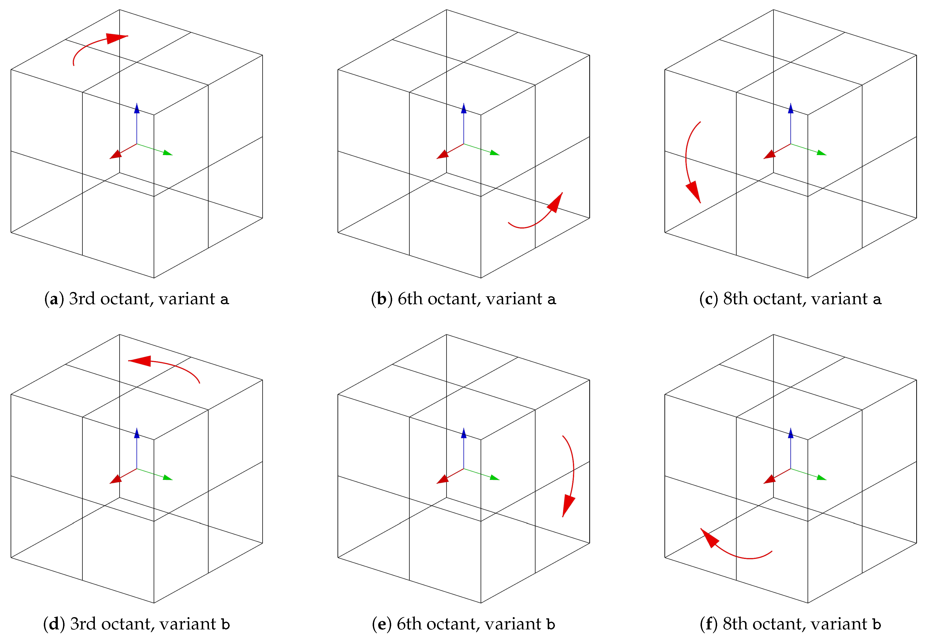
Figure A2.
Construction methods for the 7th octant.
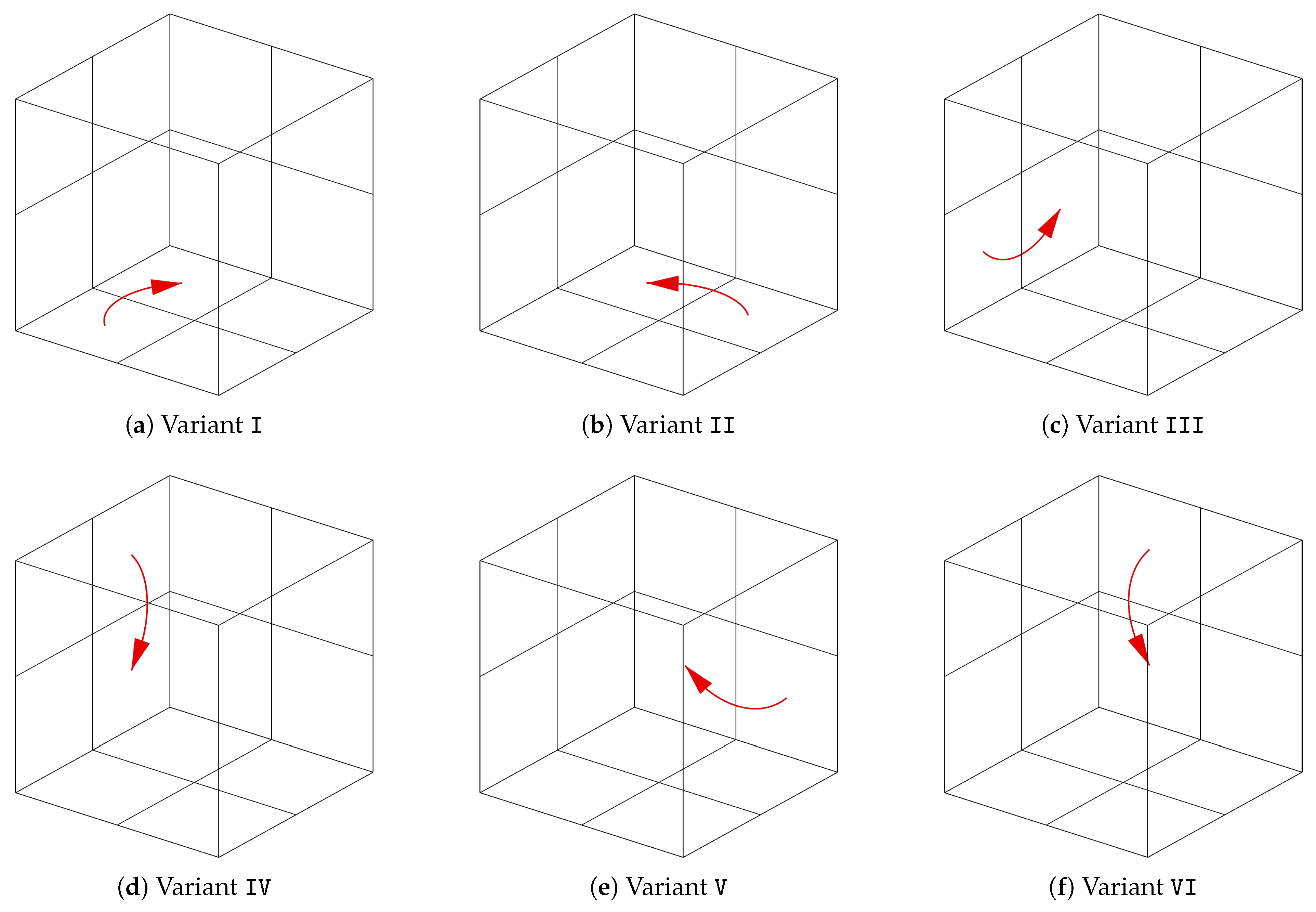
Appendix B. Unique Cell Nomenclature
Table A1.
Updated nomenclature for cells with topologies from topo_1 to topo_3.
Table A2.
Updated nomenclature for cells with topologies from topo_4 to topo_8.
Table A3.
Updated nomenclature for cells with topologies from topo_9 to topo_13.
Table A4.
Updated nomenclature for cells with topologies from topo_14 to topo_20.
Appendix C. Natural Frequencies: Comparison Between Shell Elements and Experimental Data
Table A5.
Comparison between natural frequencies with shell elements and experimental data.
References
- Ma, W.W.S.; Yang, H.; Zhao, Y.; Li, X.; Ding, J.; Qu, S.; Song, X. Multi-Physical Lattice Metamaterials Enabled by Additive Manufacturing: Design Principles, Interaction Mechanisms, and Multifunctional Applications. Adv. Sci. 2025, 12, 2405835. [Google Scholar] [CrossRef] [Scilit]
- Vassallo, F.; Buono, M.; Franchitti, S.; Borrelli, R.; Pirozzi, C.; Lamanna, G. Industrial Applications of Lattice Structures in Components Made with EBM Additive Technology. Macromol. Symp. 2022, 404, 2100518. [Google Scholar] [CrossRef] [Scilit]
- Consulting, S. Lattice Structures in Additive Manufacturing: Strength, Weight, and Performance. 2025. Available online: https://www.stratagem-consulting-llc.com/blog-2-1/blog-post-title-two-tbznc (accessed on 18 January 2026).
- Khan, N.; Riccio, A. A systematic review of design for additive manufacturing of aerospace lattice structures: Current trends and future directions. Prog. Aerosp. Sci. 2024, 149, 101021. [Google Scholar] [CrossRef] [Scilit]
- Pan, C.; Han, Y.; Lu, J. Design and optimization of lattice structures: A review. Appl. Sci. 2020, 10, 6374. [Google Scholar] [CrossRef] [Scilit]
- Yin, H.; Zhang, W.; Zhu, L.; Meng, F.; Liu, J.; Wen, G. Review on lattice structures for energy absorption properties. Compos. Struct. 2023, 304, 116397. [Google Scholar] [CrossRef] [Scilit]
- ERP. 3D Printing Lattice Structures. 2023. Available online: https://www.3erp.com/blog/3d-printing-lattice-structures/ (accessed on 18 January 2026).
- Zhou, X.; Jin, Y.; Du, J. Functionally graded scaffolds with programmable pore size distribution based on triply periodic minimal surface fabricated by selective laser melting. Materials 2020, 13, 5046. [Google Scholar] [CrossRef] [Scilit]
- Davoodi, E.; Montazerian, H.; Mirhakimi, A.S.; Zhianmanesh, M.; Ibhadode, O.; Shahabad, S.I.; Esmaeilizadeh, R.; Sarikhani, E.; Toorandaz, S.; Sarabi, S.A.; et al. Additively manufactured metallic biomaterials. Bioact. Mater. 2022, 15, 214–249. [Google Scholar] [CrossRef] [Scilit]
- Liu, F.; Ran, Q.; Zhao, M.; Zhang, T.; Zhang, D.Z.; Su, Z. Additively manufactured continuous cell-size gradient porous scaffolds: Pore characteristics, mechanical properties and biological responses in vitro. Materials 2020, 13, 2589. [Google Scholar] [CrossRef] [Scilit]
- Dutkowski, K.; Kruzel, M.; Rokosz, K. Review of the state-of-the-art uses of minimal surfaces in heat transfer. Energies 2022, 15, 7994. [Google Scholar] [CrossRef] [Scilit]
- Yeranee, K.; Rao, Y. A review of recent investigations on flow and heat transfer enhancement in cooling channels embedded with triply periodic minimal surfaces (TPMS). Energies 2022, 15, 8994. [Google Scholar] [CrossRef] [Scilit]
- Ali, M.; Sajjad, U.; Hussain, I.; Abbas, N.; Ali, H.M.; Yan, W.M.; Wang, C.C. On the assessment of the mechanical properties of additively manufactured lattice structures. Eng. Anal. Bound. Elem. 2022, 142, 93–116. [Google Scholar] [CrossRef] [Scilit]
- Han, S.C.; Lee, J.W.; Kang, K. A New Type of Low Density Material: Shellular. Adv. Mater. 2015, 27, 5506–5511. [Google Scholar] [CrossRef] [Scilit] [PubMed]
- Bonatti, C.; Mohr, D. Smooth-shell metamaterials of cubic symmetry: Anisotropic elasticity, yield strength and specific energy absorption. Acta Mater. 2019, 164, 301–321. [Google Scholar] [CrossRef] [Scilit]
- Wang, Y.; Zhang, X.; Li, Z.; Gao, H.; Li, X. Achieving the theoretical limit of strength in shell-based carbon nanolattices. Proc. Natl. Acad. Sci. USA 2022, 119, e2119536119. [Google Scholar] [CrossRef] [Scilit]
- Al-Ketan, O.; Rowshan, R.; Al-Rub, R.K.A. Topology-mechanical property relationship of 3D printed strut, skeletal, and sheet based periodic metallic cellular materials. Addit. Manuf. 2018, 19, 167–183. [Google Scholar] [CrossRef] [Scilit]
- Ahmed, N.; Barsoum, I.; Abu Al-Rub, R.K. Numerical investigation on the effect of residual stresses on the effective mechanical properties of 3D-printed TPMS lattices. Metals 2022, 12, 1344. [Google Scholar] [CrossRef] [Scilit]
- Lee, M.G.; Lee, J.W.; Han, S.C.; Kang, K. Mechanical analyses of “Shellular”, an ultralow-density material. Acta Mater. 2016, 103, 595–607. [Google Scholar] [CrossRef] [Scilit]
- Tancogne-Dejean, T.; Diamantopoulou, M.; Gorji, M.B.; Bonatti, C.; Mohr, D. 3D plate-lattices: An emerging class of low-density metamaterial exhibiting optimal isotropic stiffness. Adv. Mater. 2018, 30, 1803334. [Google Scholar] [CrossRef] [Scilit]
- Sajjad, U.; Rehman, T.u.; Ali, M.; Park, C.W.; Yan, W.M. Manufacturing and potential applications of lattice structures in thermal systems: A comprehensive review of recent advances. Int. J. Heat Mass Transf. 2022, 198, 123352. [Google Scholar] [CrossRef] [Scilit]
- Schwarz, H.A. Gesammelte Mathematische Abhandlungen; American Mathematical Soc.: Providence, RI, USA, 1972; Volume 260. [Google Scholar]
- Neovius, E.R. Bestimmung Zweier Speciellen Periodischen Minimalflächen auf Welchen Unendlich Viele Gerade Linien und Unendlich Viele Ebene Geodätische Linien Liegen: Akademische Abhandlung; Frenckell: Helsinki, Finland, 1883. [Google Scholar]
- Schoen, A.H. Infinite Periodic Minimal Surfaces Without Self-Intersections; National Aeronautics and Space Administration: Washington, DC, USA, 1970; Volume 5541. [Google Scholar]
- Toda, M.; Güler, E. Generalized Weierstrass–Enneper representation for minimal surfaces in R4. AIMS Math. 2025, 10, 22406–22420. [Google Scholar] [CrossRef] [Scilit]
- Meeks, W.H., III. The Geometry and the Conformal Structure of Triply Periodic Minimal Surfaces in R3. Ph.D. Thesis, University of California, Berkeley, CA, USA, 1975. [Google Scholar]
- Karcher, H. The triply periodic minimal surfaces of Alan Schoen and their constant mean curvature companions. Manuscripta Math. 1989, 64, 291–357. [Google Scholar] [CrossRef] [Scilit]
- Xu, Y.; Pan, H.; Wang, R.; Du, Q.; Lu, L. New families of triply periodic minimal surface-like shell lattices. Addit. Manuf. 2023, 77, 103779. [Google Scholar] [CrossRef] [Scilit]
- Palmer, D.; Smirnov, D.; Wang, S.; Chern, A.; Solomon, J. Deepcurrents: Learning implicit representations of shapes with boundaries. In Proceedings of the IEEE/CVF Conference on Computer Vision and Pattern Recognition, New Orleans, LA, USA, 18–24 June 2022; pp. 18665–18675. [Google Scholar]
- Bouaziz, S.; Martin, S.; Liu, T.; Kavan, L.; Pauly, M. Projective dynamics: Fusing constraint projections for fast simulation. ACM Trans. Graph. 2014, 33, 1–11. [Google Scholar] [CrossRef] [Scilit]
- Boyd, S.; Parikh, N.; Chu, E.; Peleato, B.; Eckstein, J. Distributed optimization and statistical learning via the alternating direction method of multipliers. Found. Trends Mach. Learn. 2011, 3, 1–122. [Google Scholar] [CrossRef] [Scilit]
- Cromwell, P.R. Polyhedra; Cambridge University Press: Cambridge, UK, 1997; p. 295. [Google Scholar]
- Saghir, M.Z.; Yahya, M. Convection Heat Transfer and Performance Analysis of a Triply Periodic Minimal Surface (TPMS) for a Novel Heat Exchanger. Energies 2024, 17, 4275. [Google Scholar] [CrossRef] [Scilit]
- Beer, M.; Rybár, R. Numerical Study of Fluid Flow in a Gyroid-Shaped Heat Transfer Element. Energies 2024, 17, 2244. [Google Scholar] [CrossRef] [Scilit]
- Yan, G.; Sun, M.; Zhang, Z.; Liang, Y.; Jiang, N.; Pang, X.; Song, Y.; Liu, Y.; Zhao, J. Experimental study on flow and heat transfer performance of triply periodic minimal surface structures and their hybrid form as disturbance structure. Int. Commun. Heat Mass Transf. 2023, 147, 106942. [Google Scholar] [CrossRef] [Scilit]
- Silva, C.; Pais, A.I.; Caldas, G.; Gouveia, B.P.; Alves, J.L.; Belinha, J. Study on 3D printing of gyroid-based structures for superior structural behaviour. Prog. Addit. Manuf. 2021, 6, 689–703. [Google Scholar] [CrossRef] [Scilit]
- Lohmuller, P.; Favre, J.; Piotrowski, B.; Kenzari, S.; Laheurte, P. Stress concentration and mechanical strength of cubic lattice architectures. Materials 2018, 11, 1146. [Google Scholar] [CrossRef] [Scilit] [PubMed]
- Gao, S.; Liu, W.; Zhang, L.; Gain, A.K. A new polymer-based mechanical metamaterial with tailorable large negative Poisson’s ratios. Polymers 2020, 12, 1492. [Google Scholar] [CrossRef] [Scilit]
- Grygier, D.; Kurzawa, A.; Stachowicz, M.; Krawiec, K.; Stępczak, M.; Roszak, M.; Kazimierczak, M.; Aniszewska, D.; Pyka, D. Investigations into the Material Characteristics of Selected Plastics Manufactured Using SLA-Type Additive Methods. Polymers 2024, 16, 1607. [Google Scholar] [CrossRef] [Scilit] [PubMed]
- Bercin, A.; Tanaka, M. Coupled flexural–torsional vibrations of Timoshenko beams. J. Sound Vib. 1997, 207, 47–59. [Google Scholar] [CrossRef] [Scilit]
- Schmutzler, C.; Stiehl, T.H.; Zaeh, M.F. Empirical process model for shrinkage-induced warpage in 3D printing. Rapid Prototyp. J. 2019, 25, 721–727. [Google Scholar] [CrossRef] [Scilit]
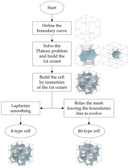
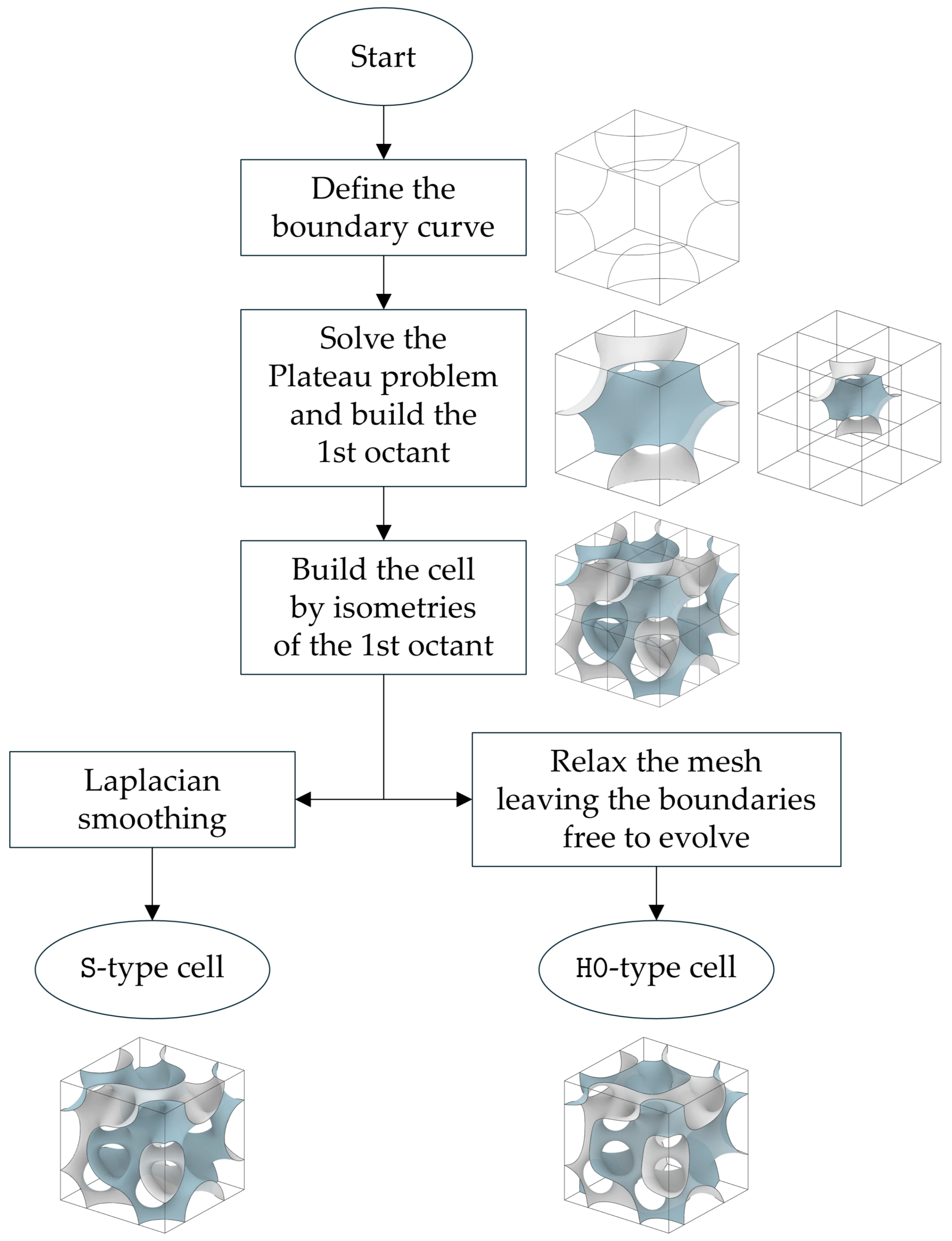
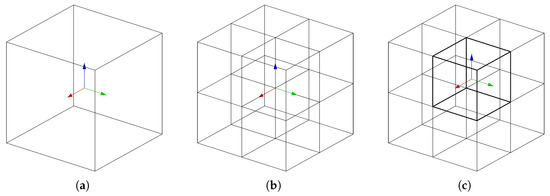
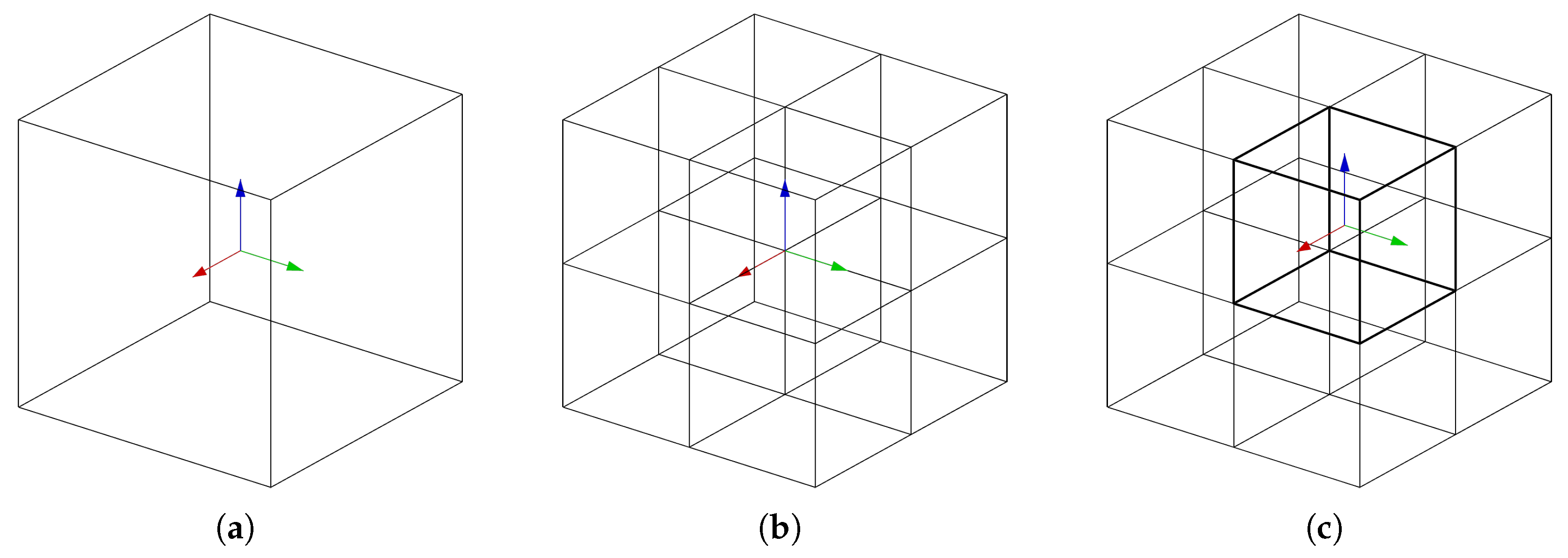
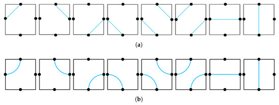
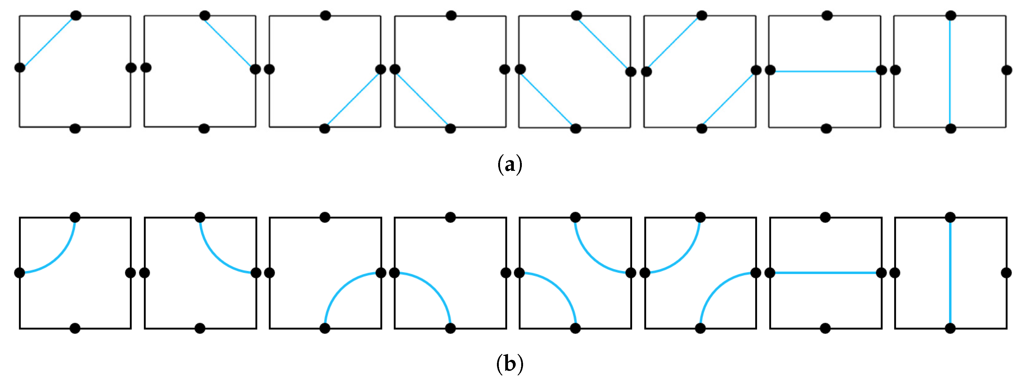
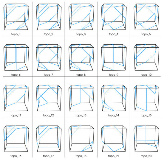
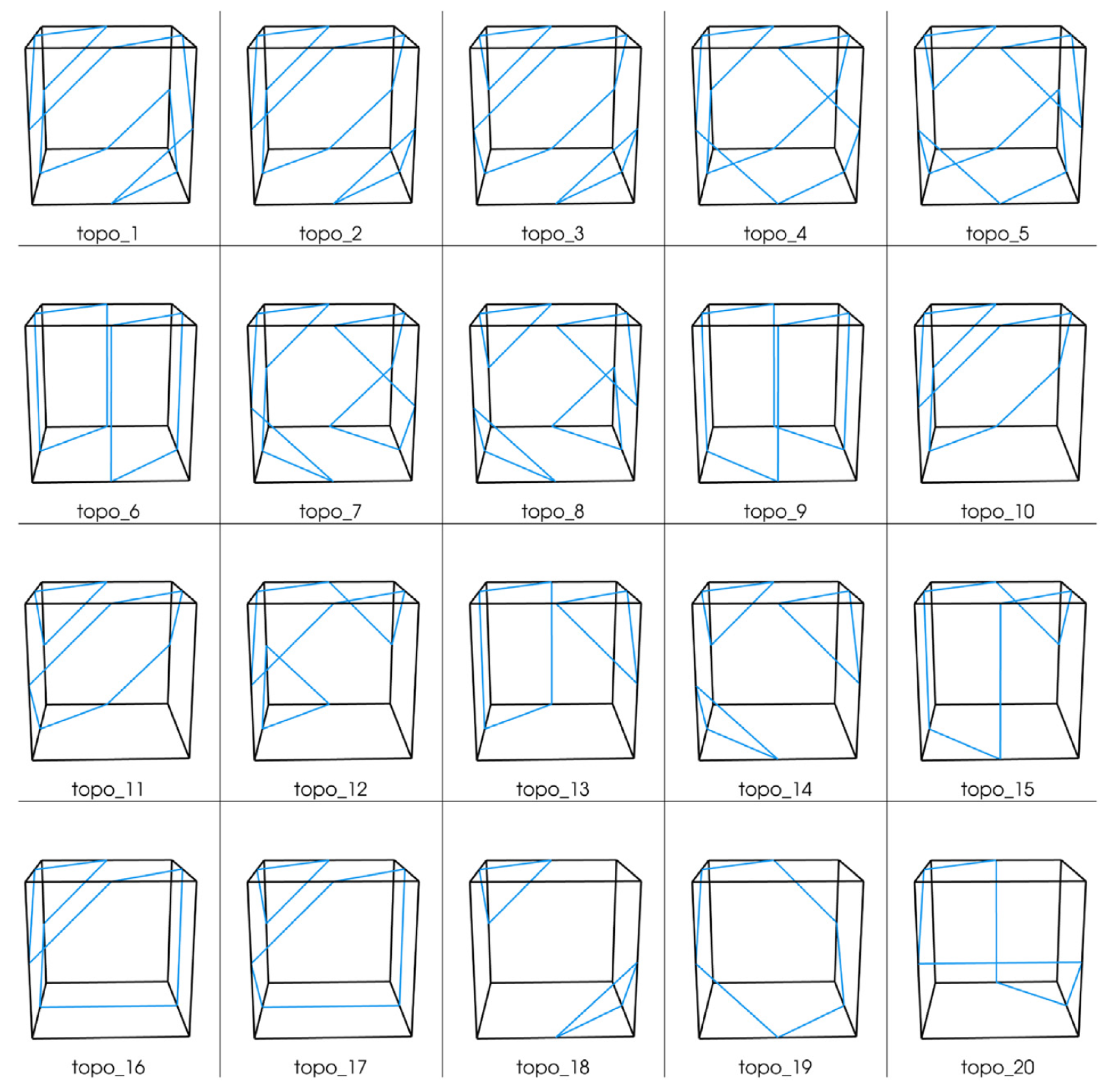
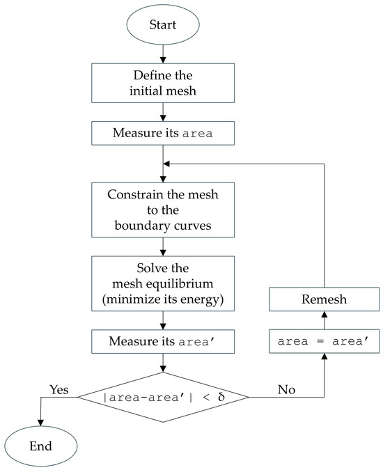
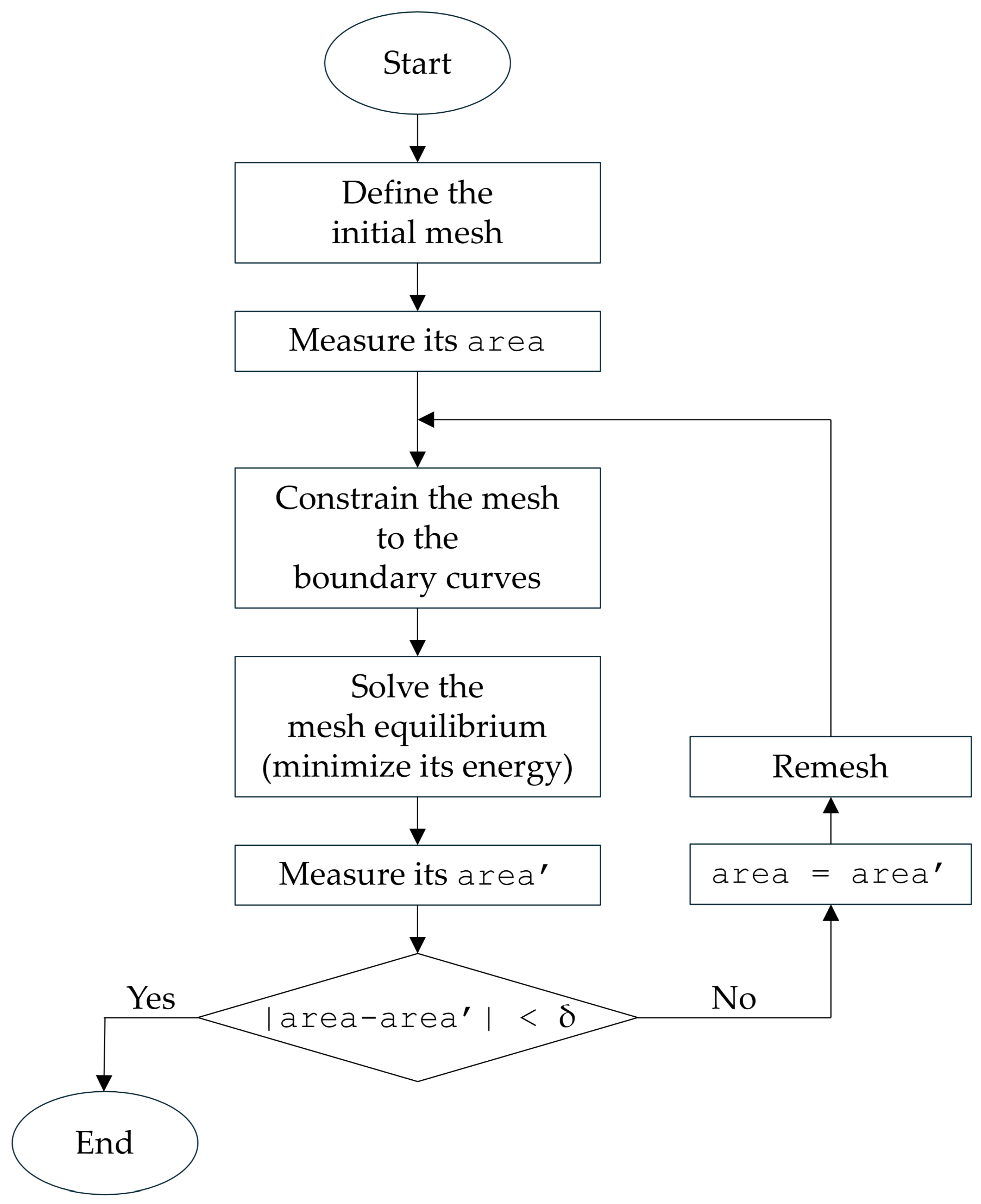
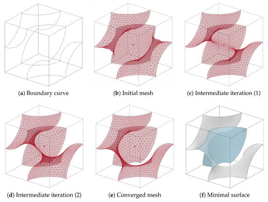
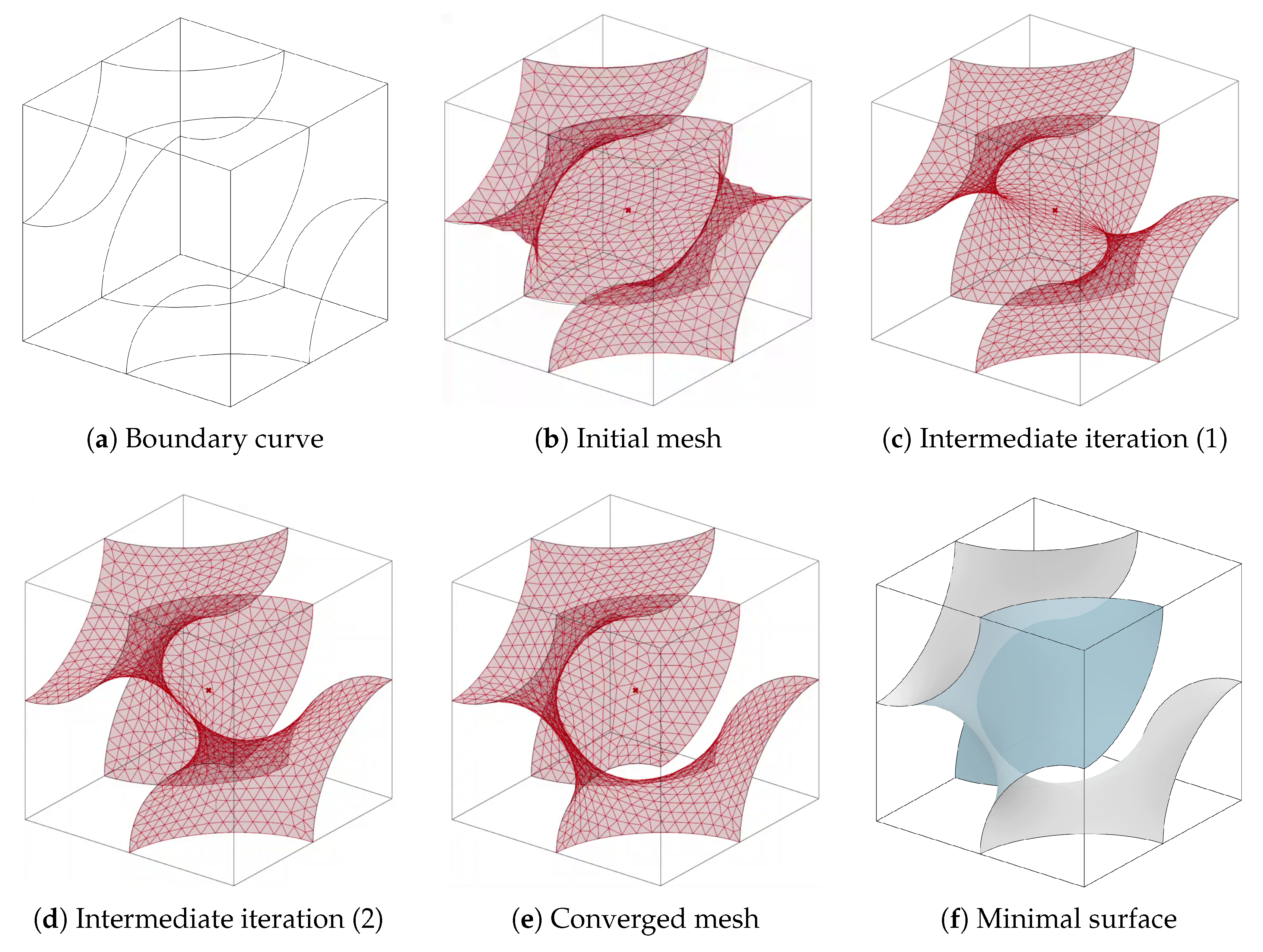
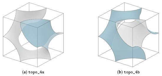
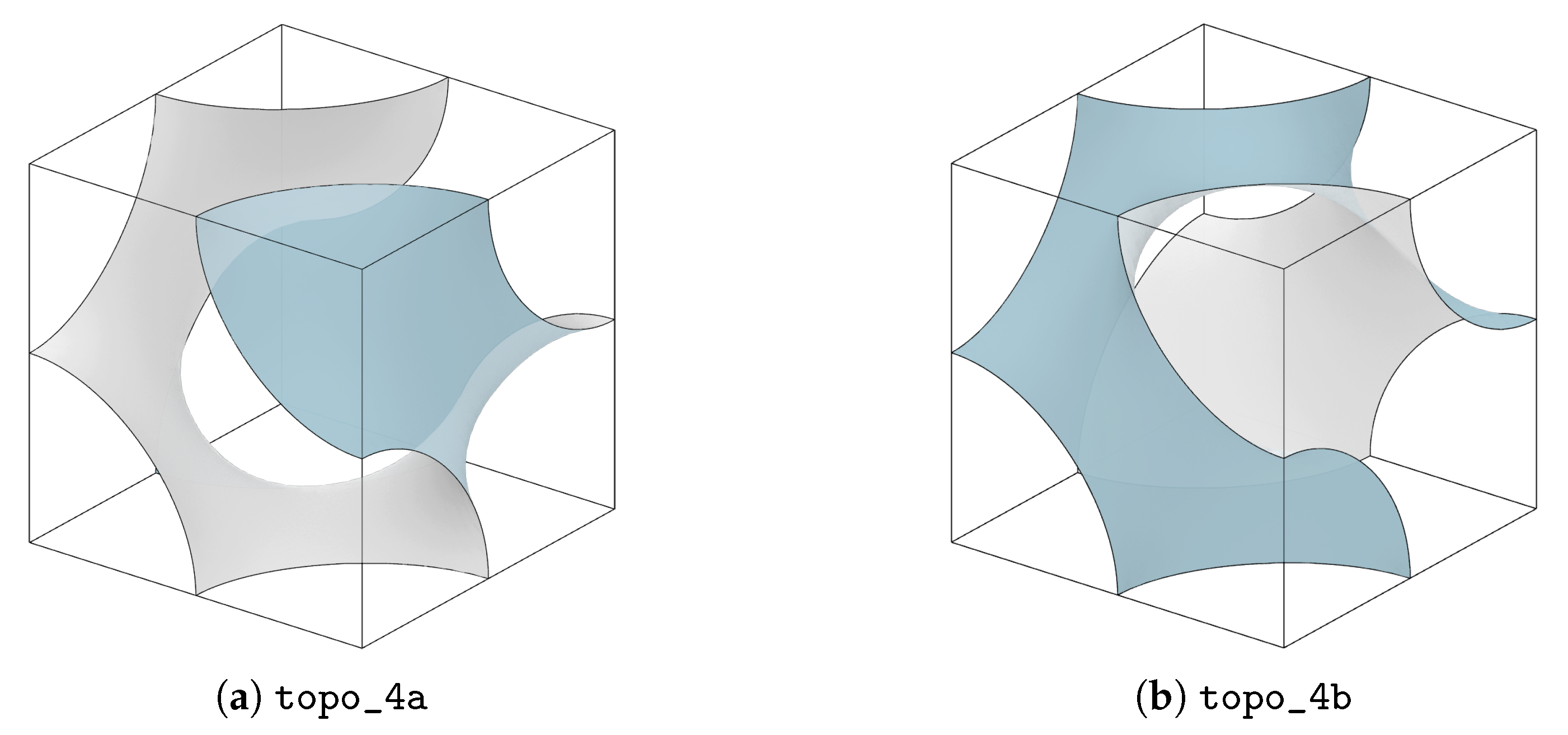
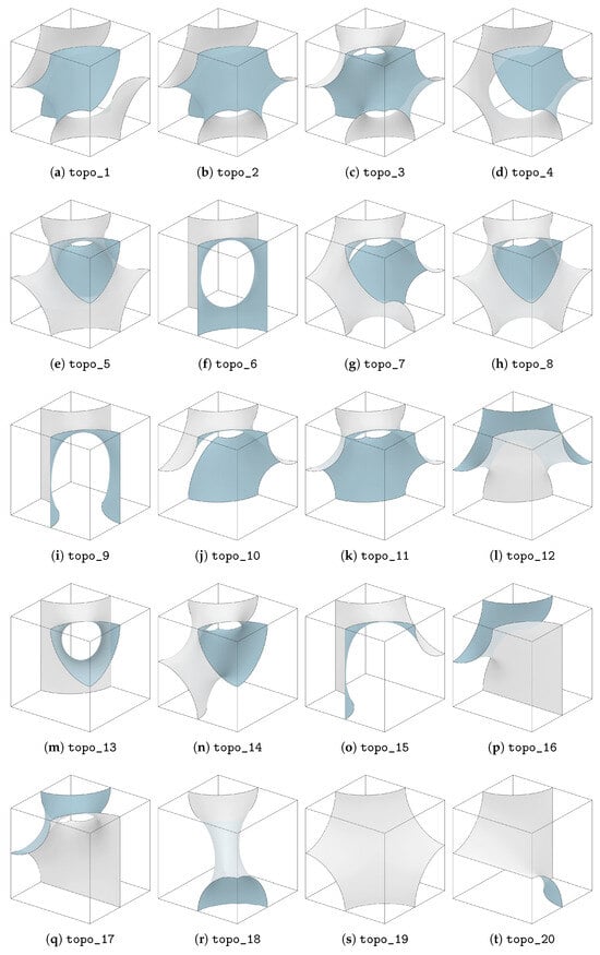
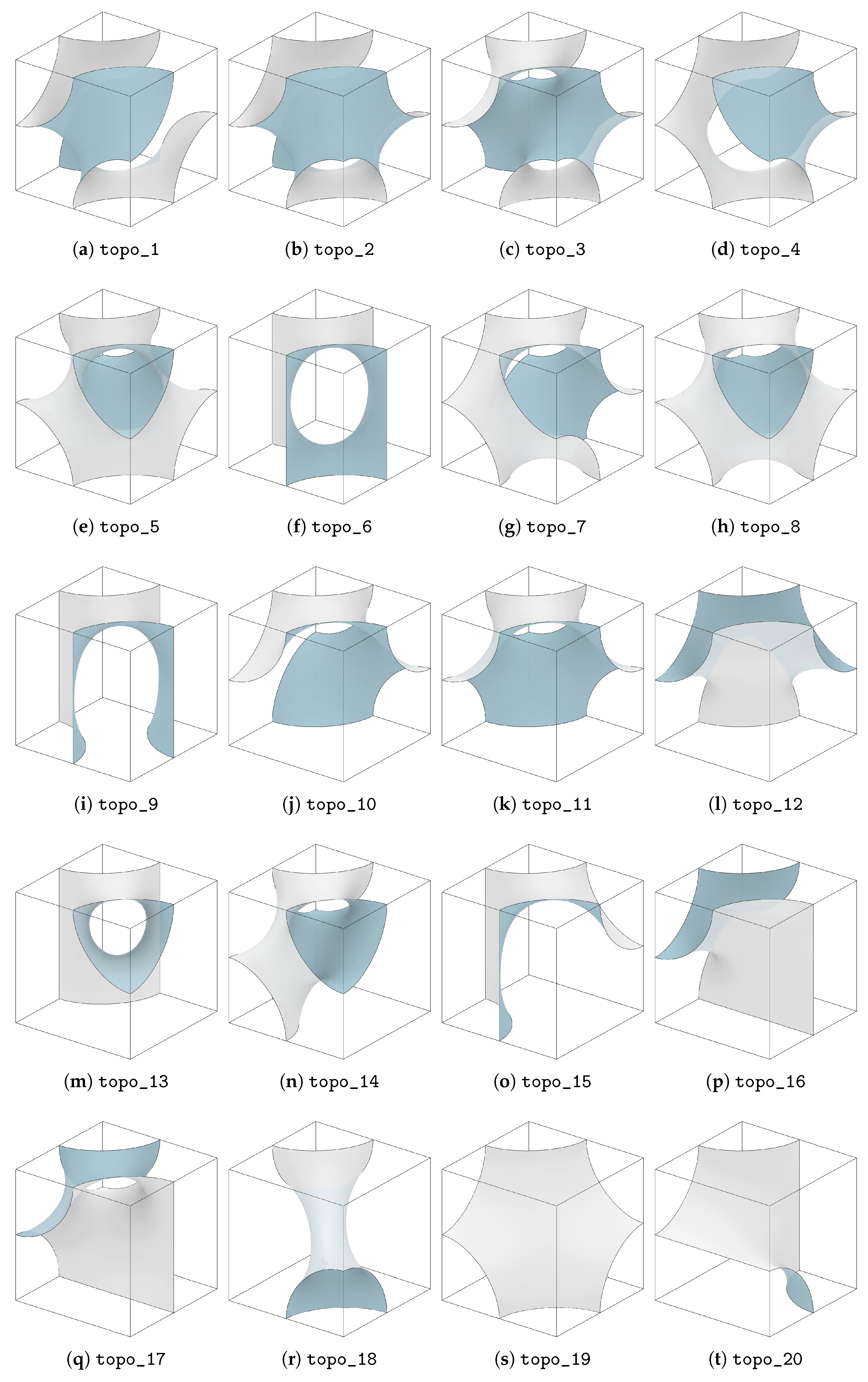
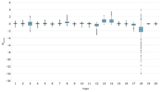
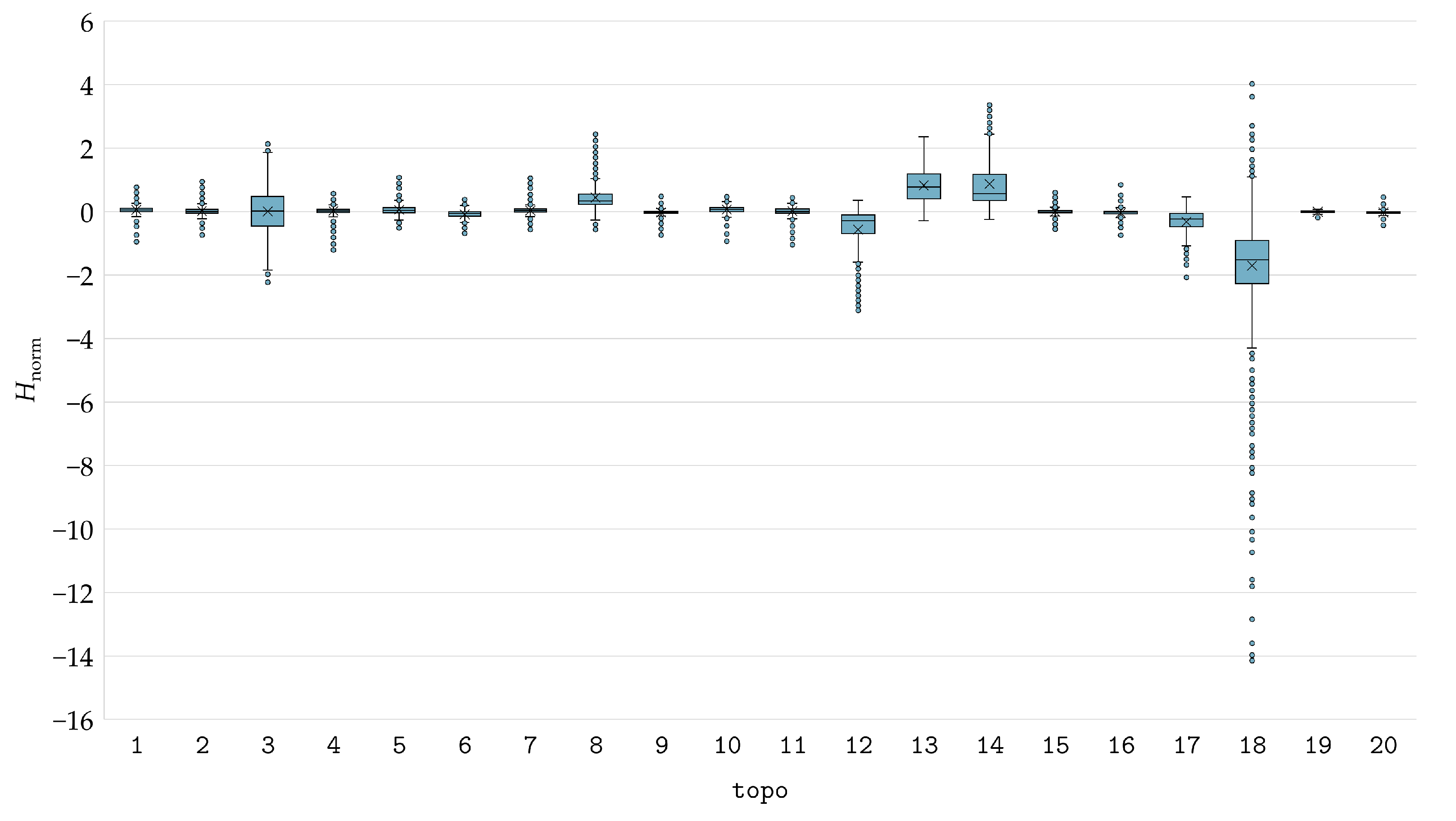
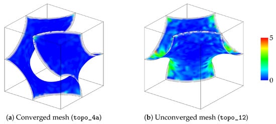
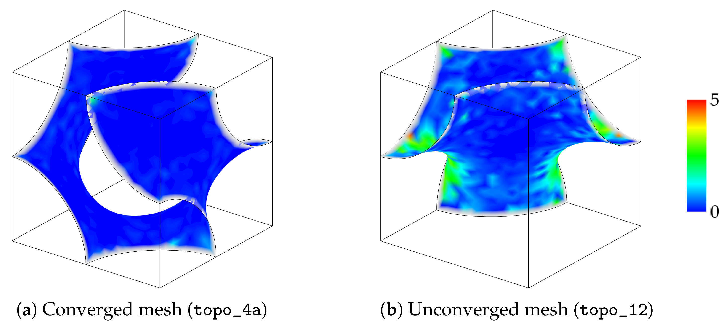
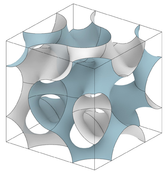
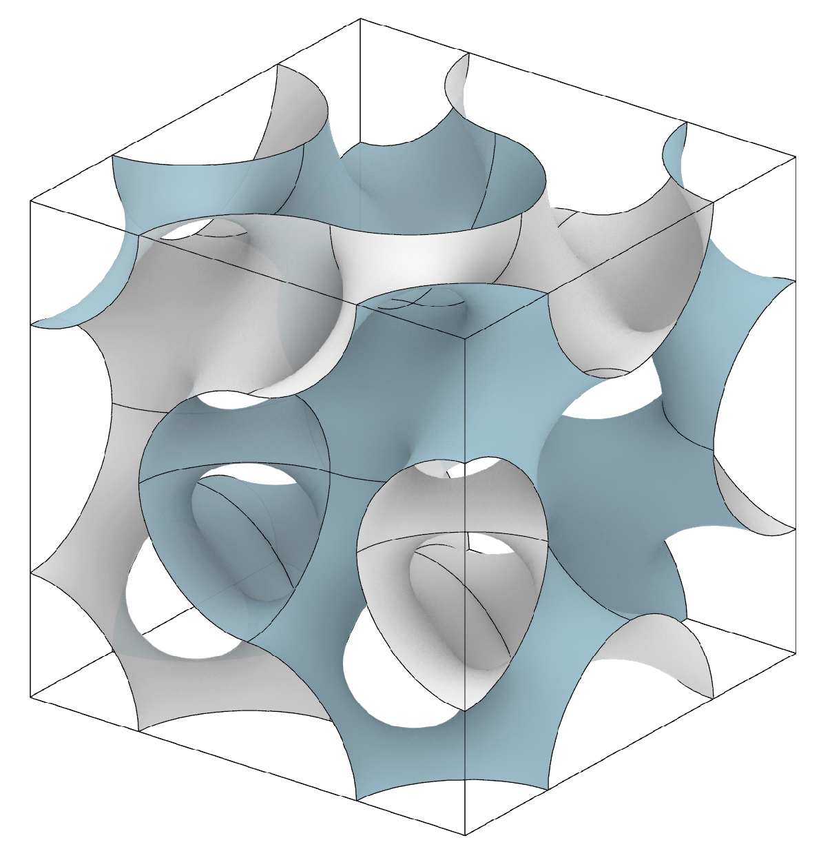
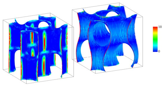
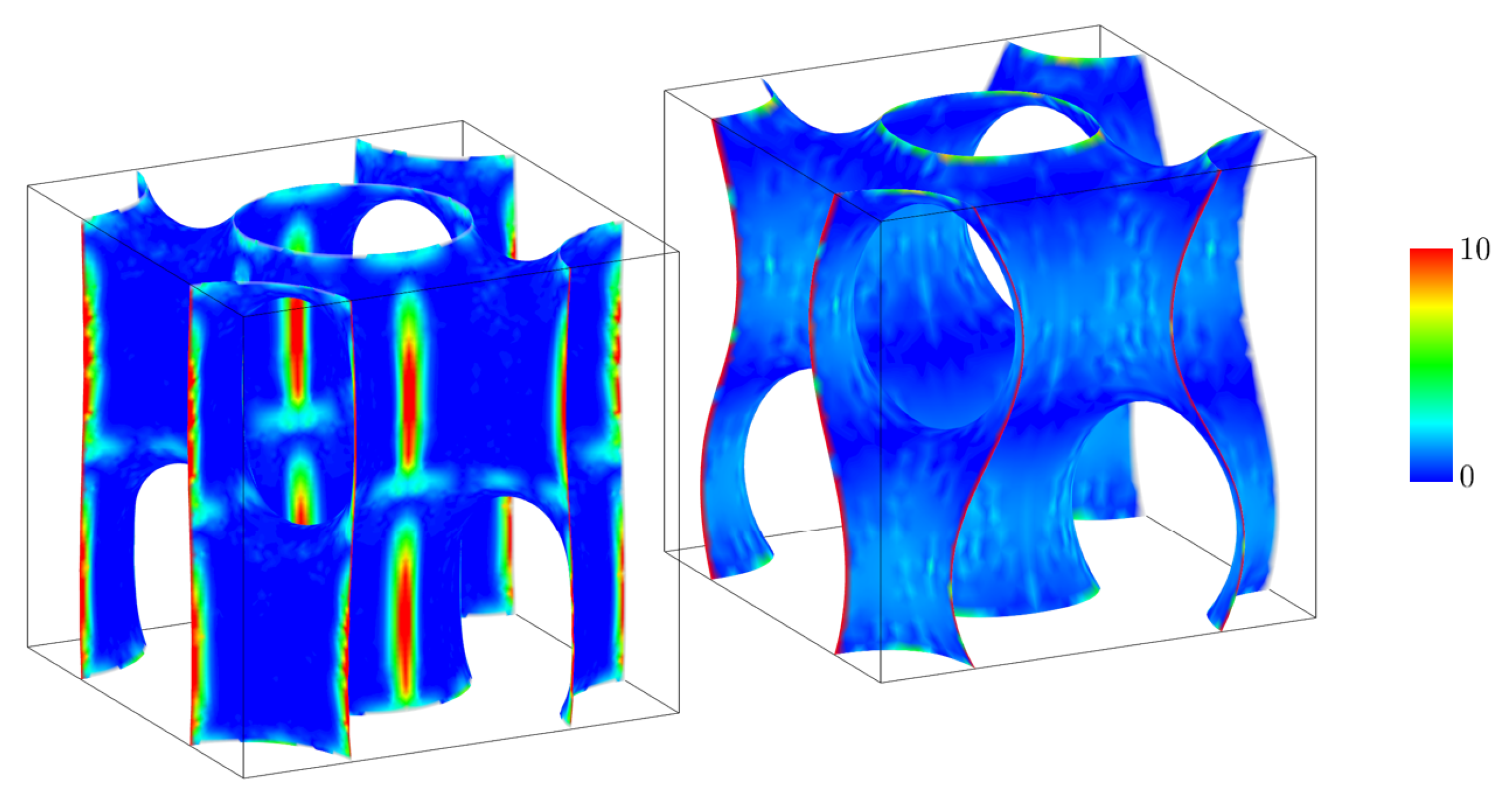
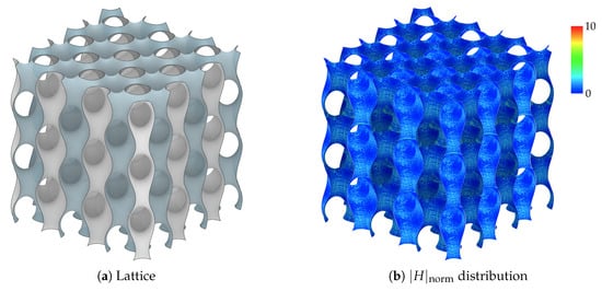
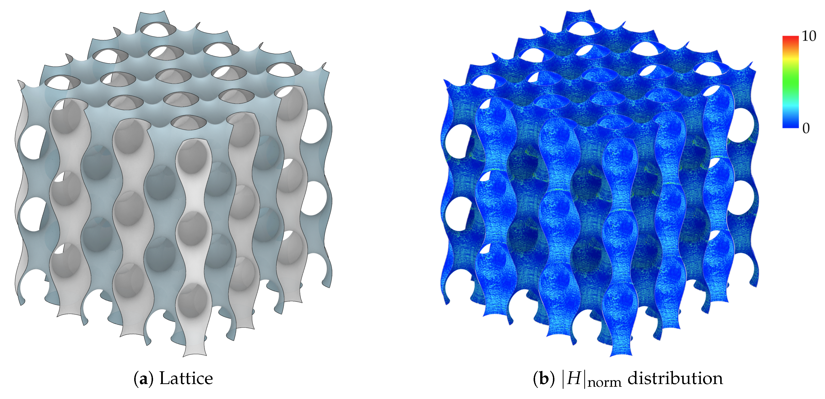
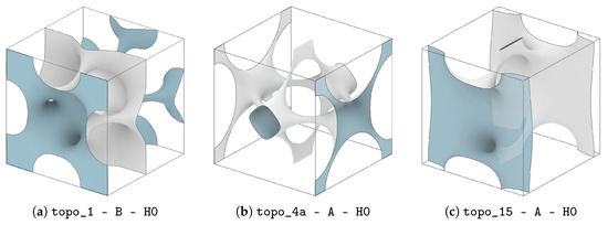
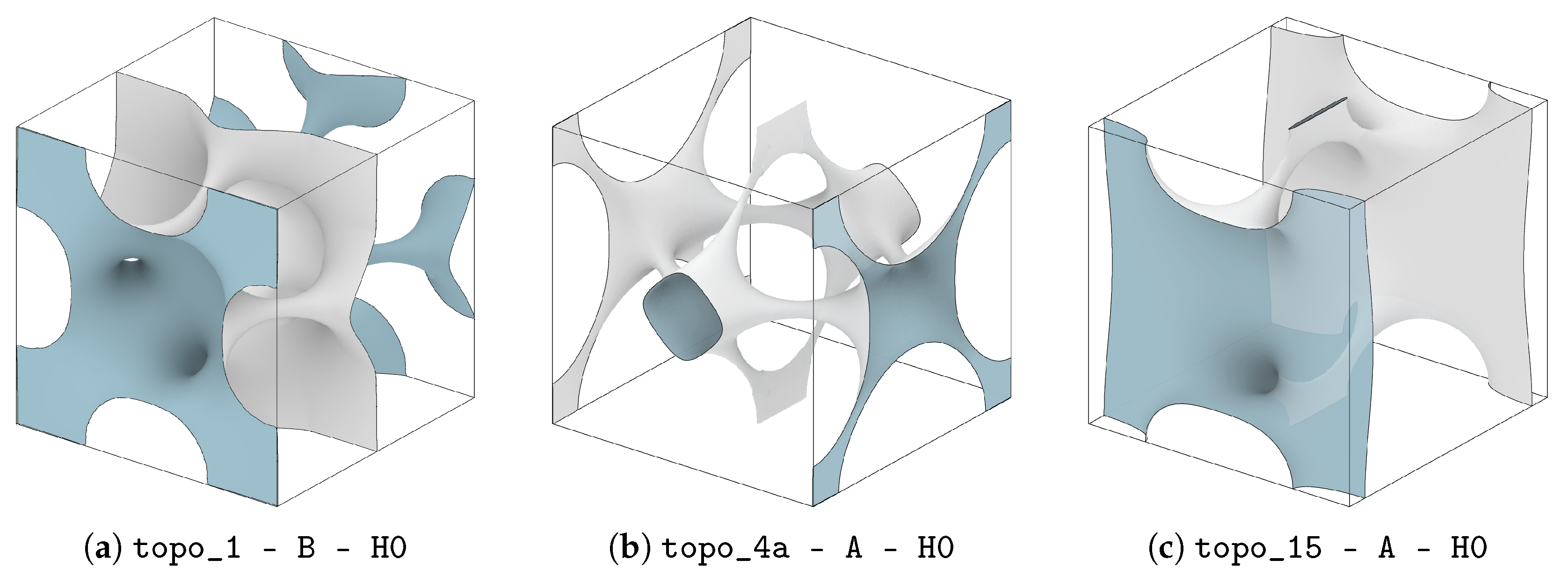
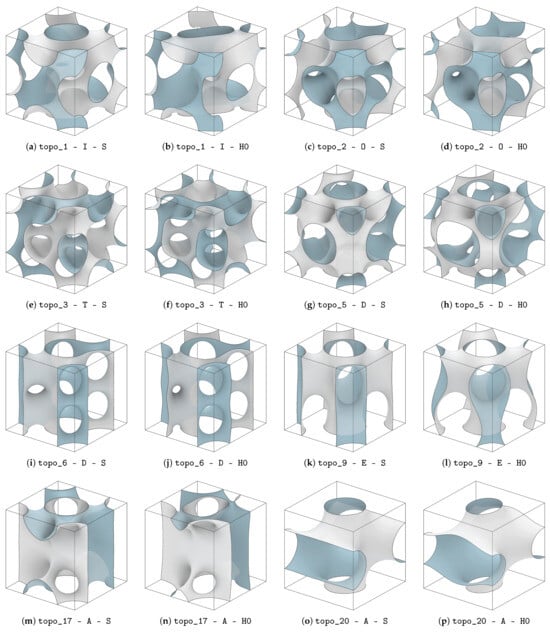
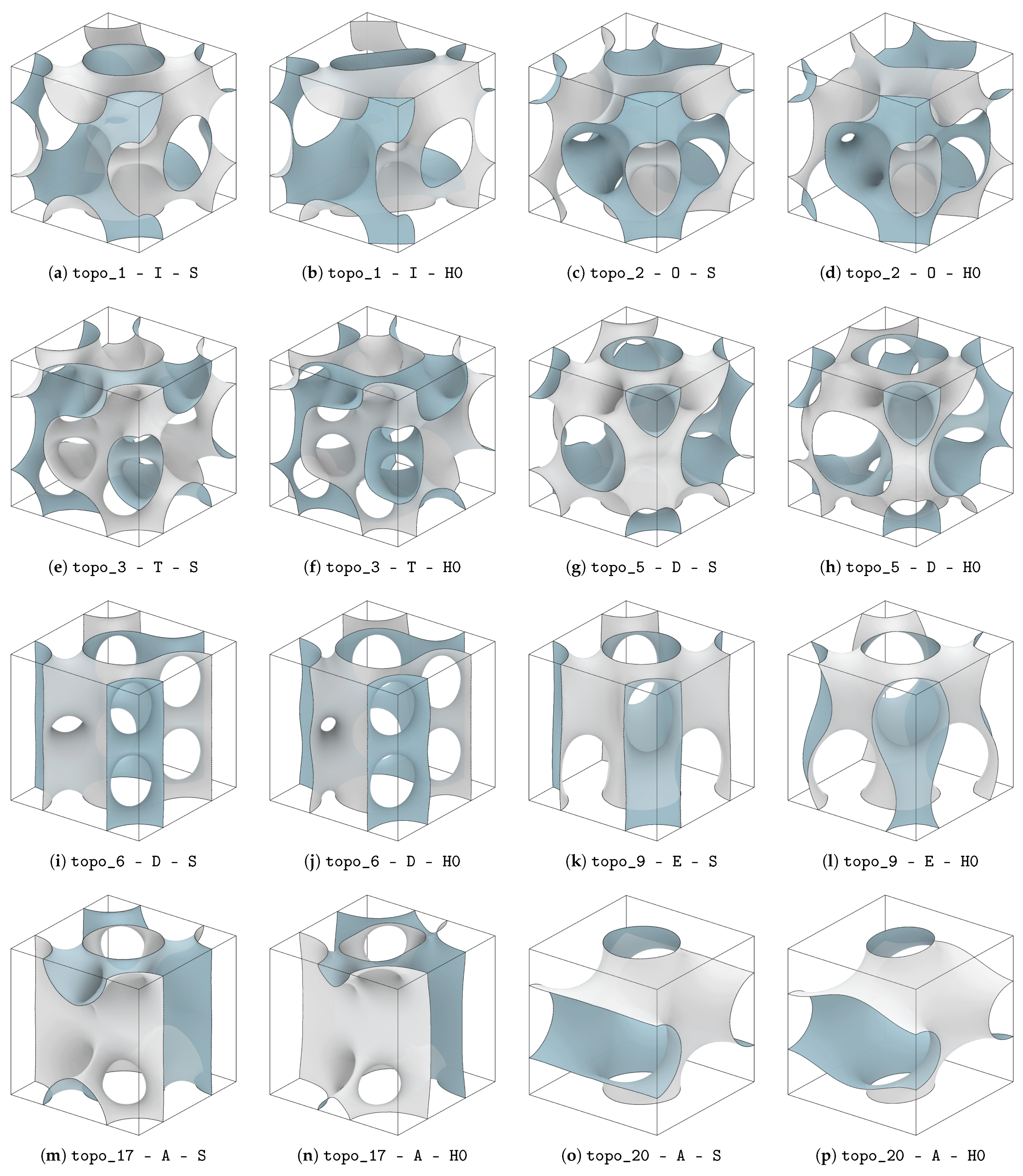
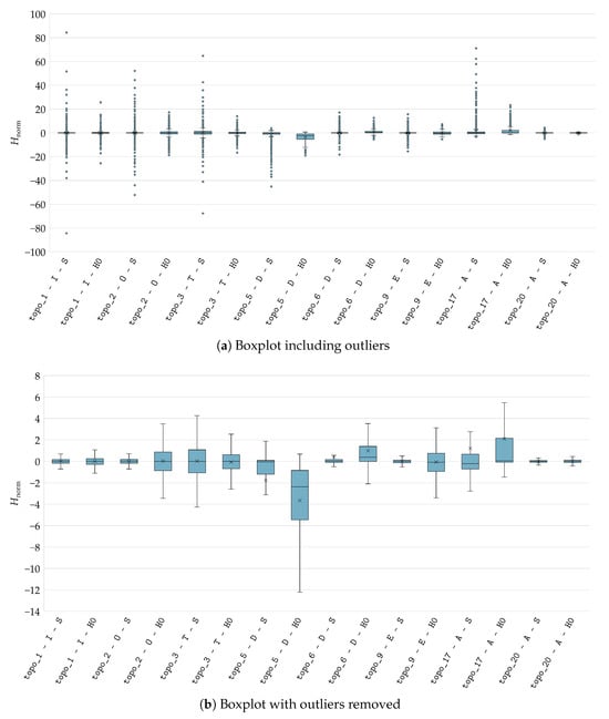
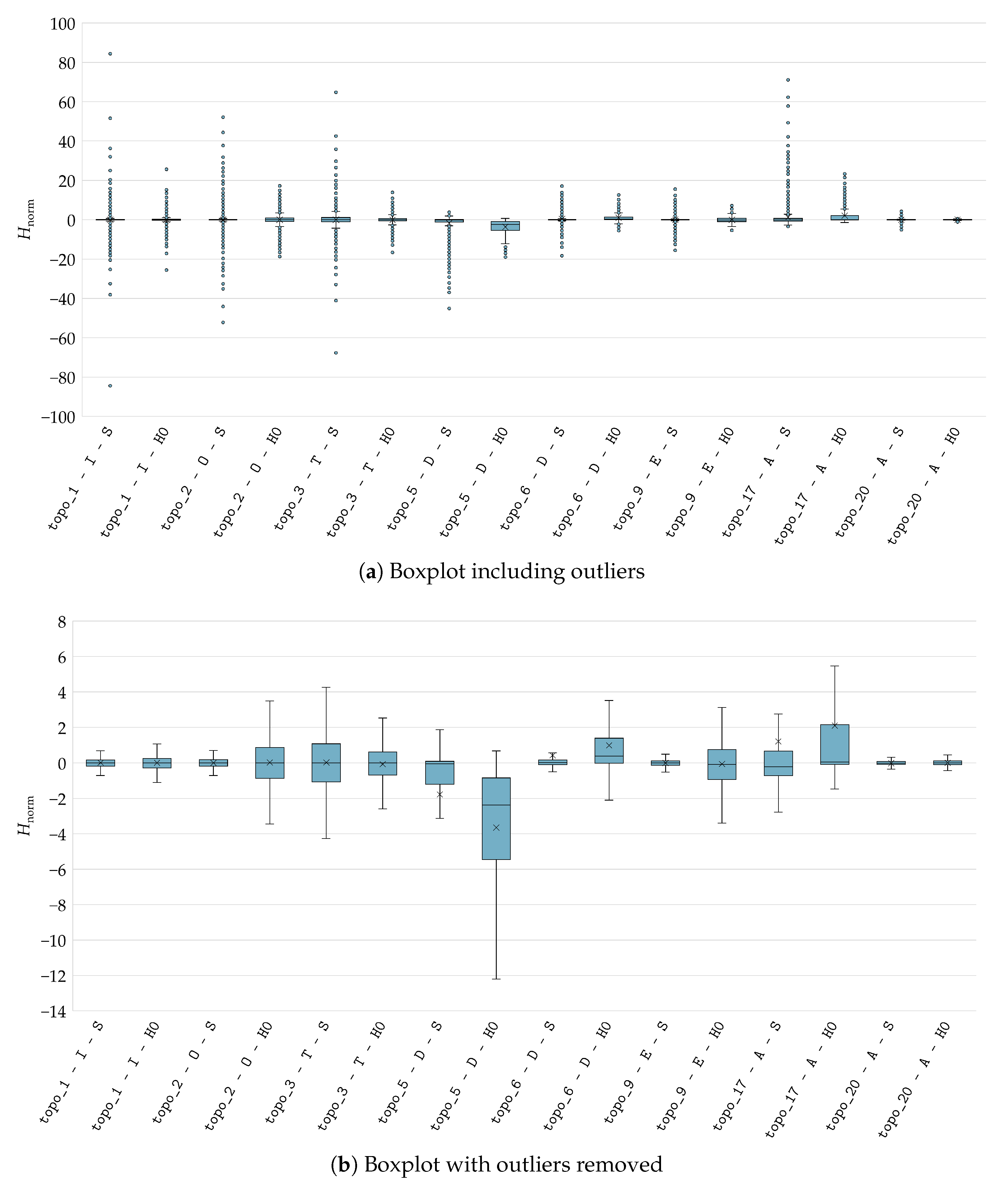
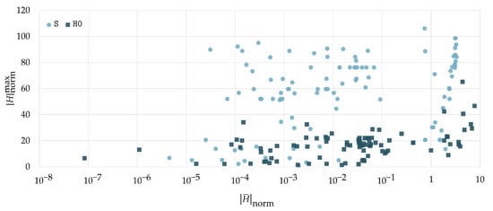
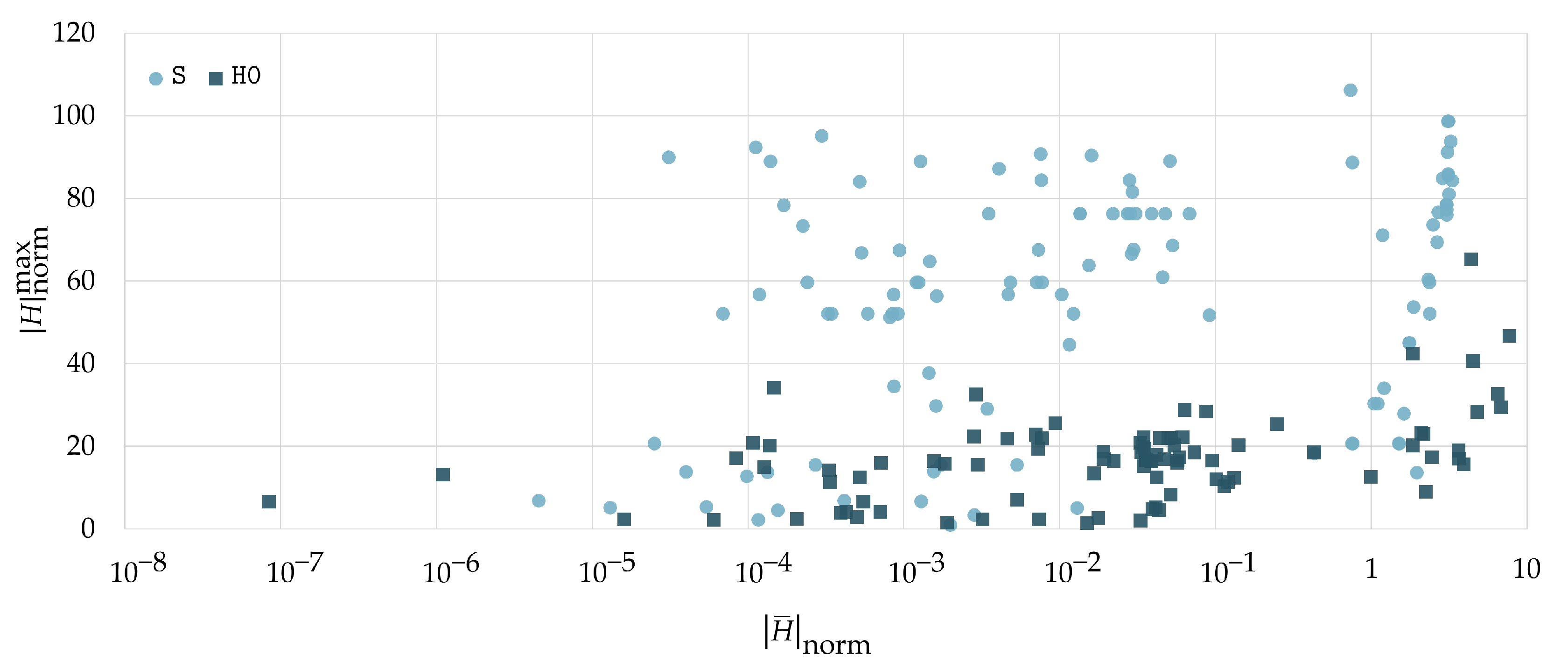
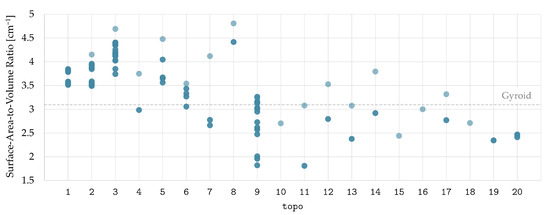
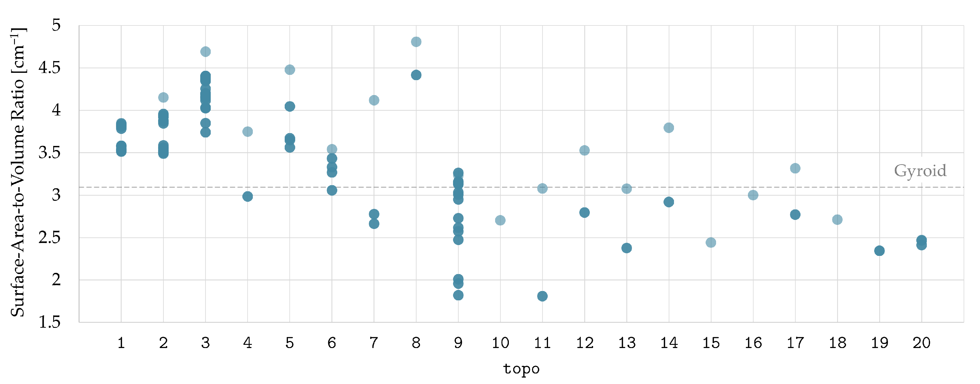
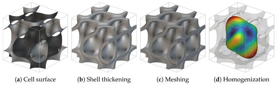
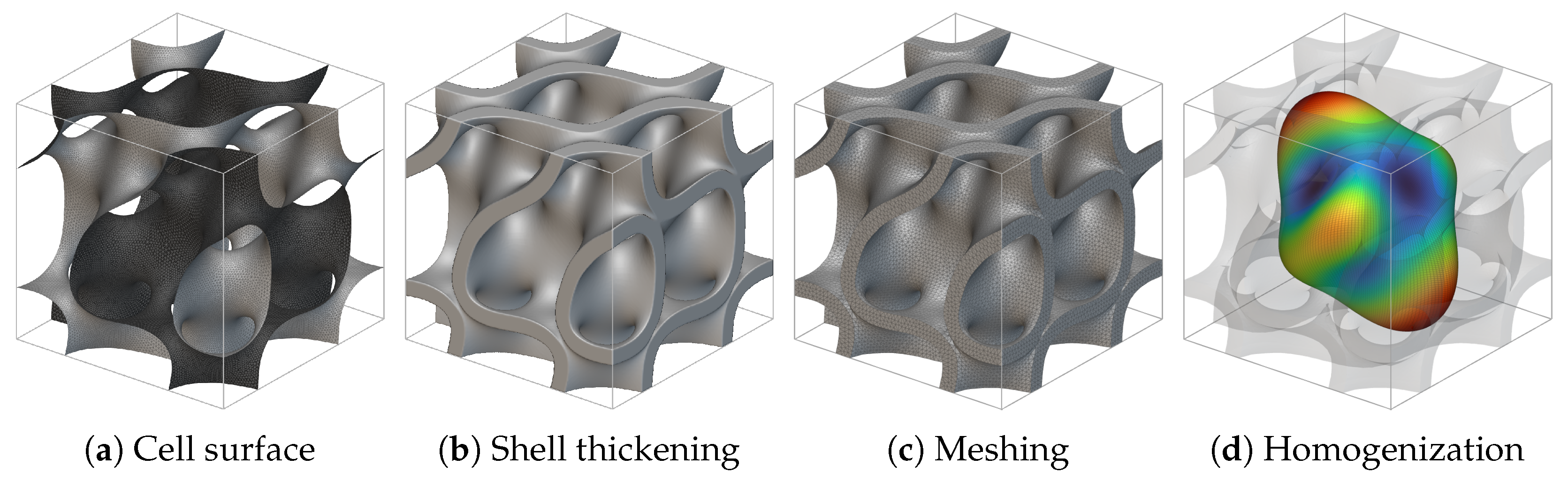
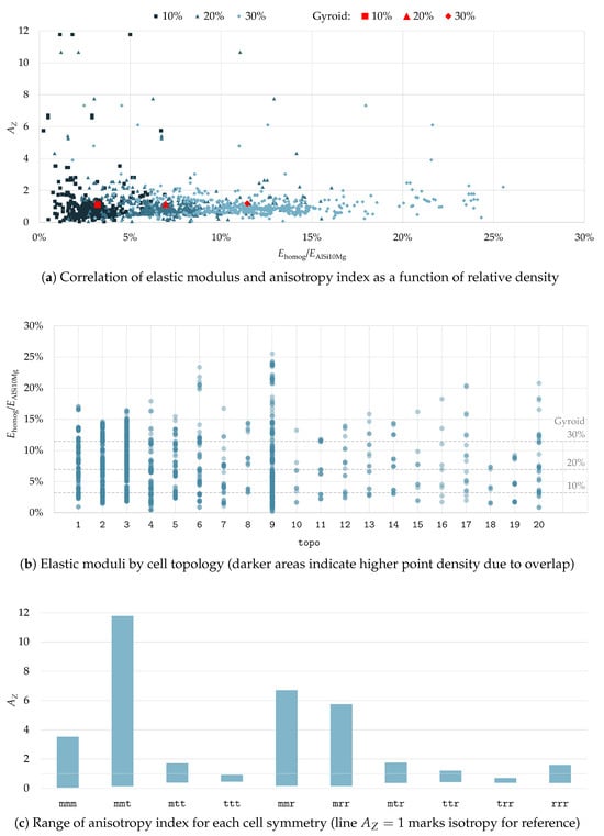
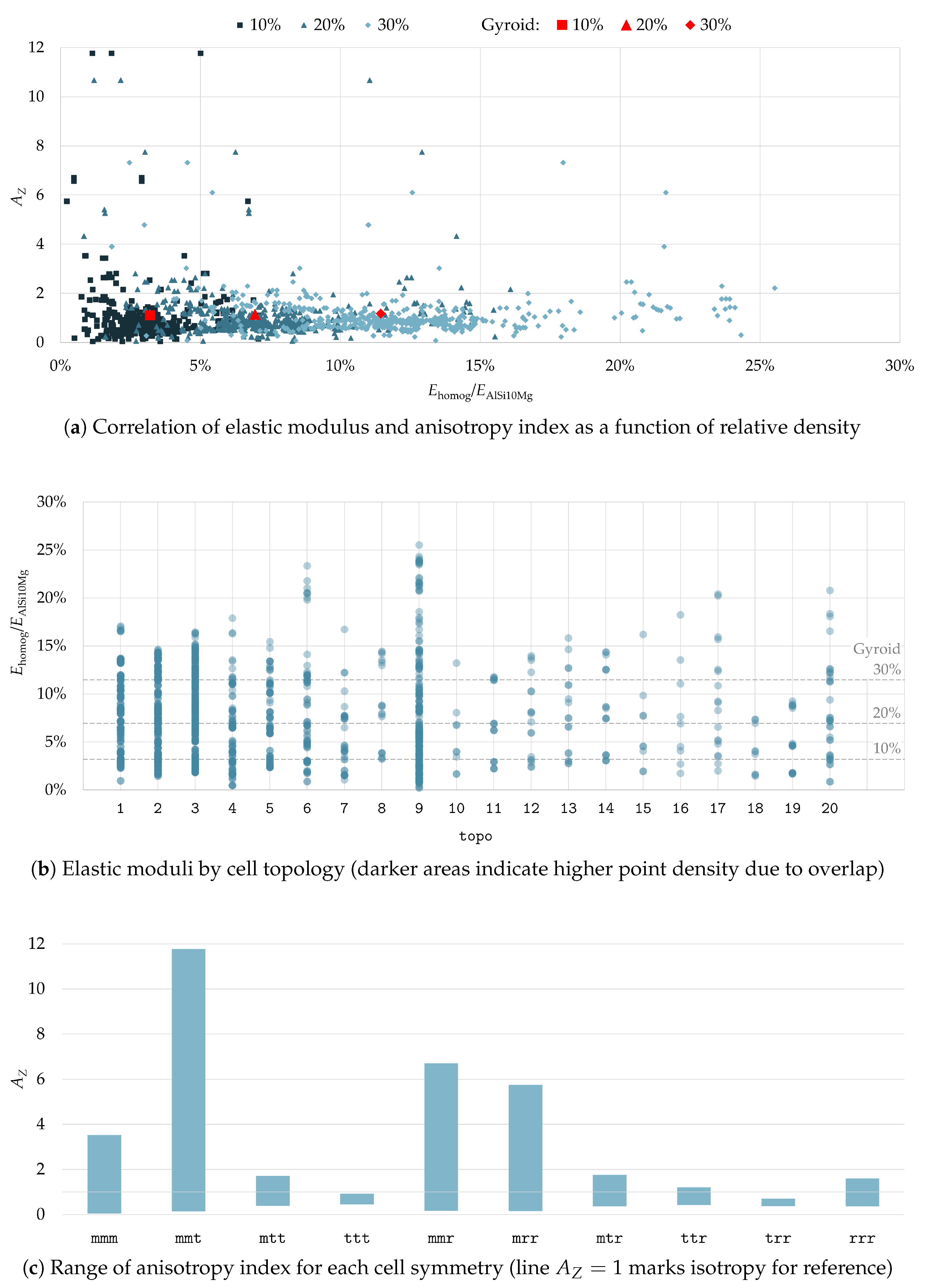
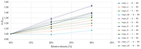
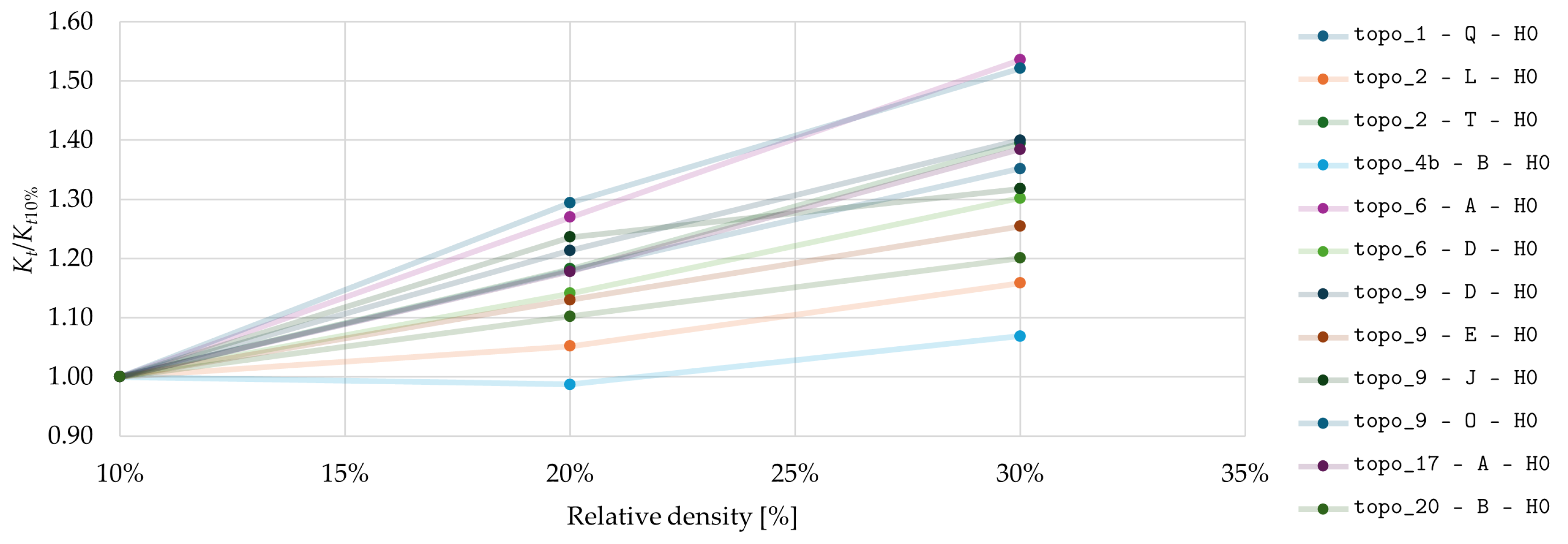
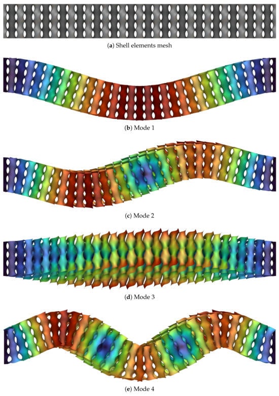
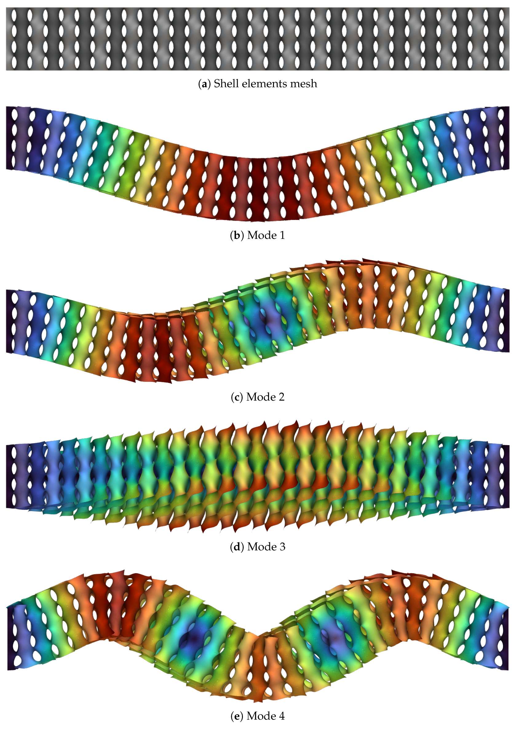
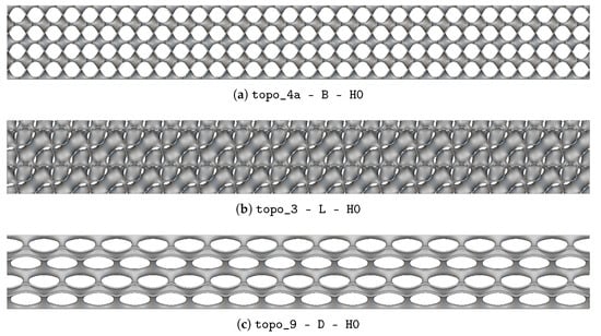
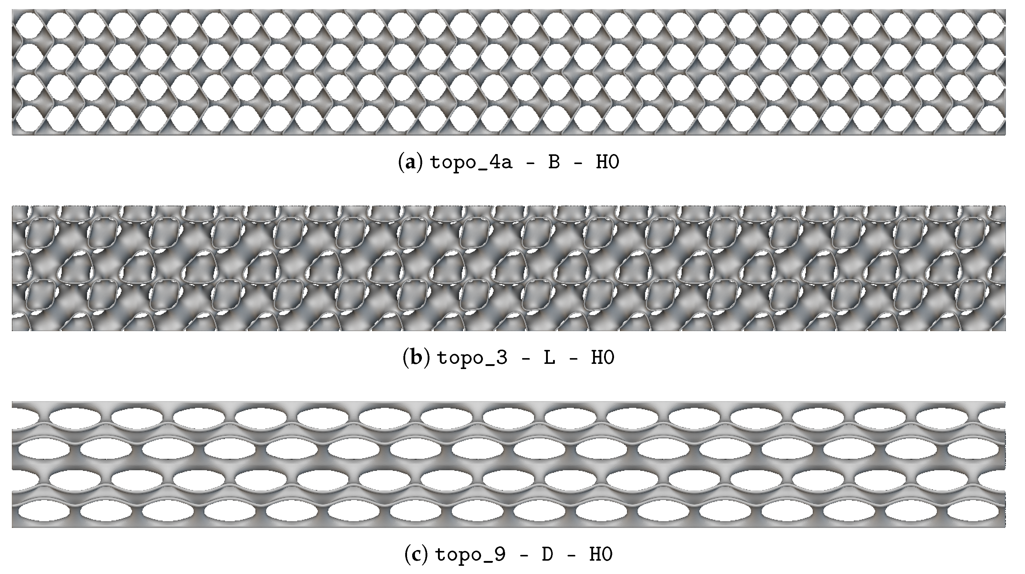
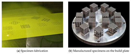
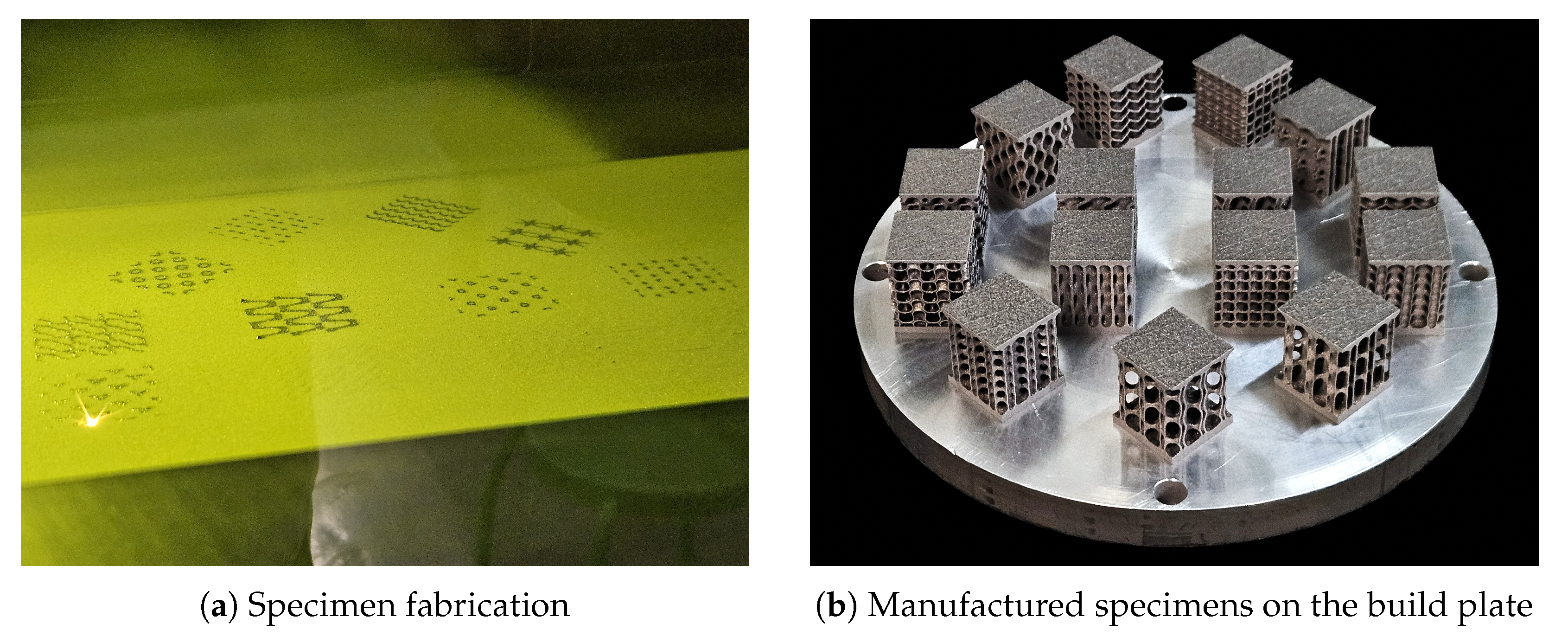
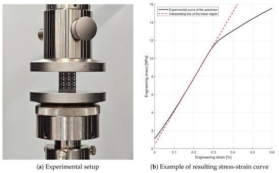
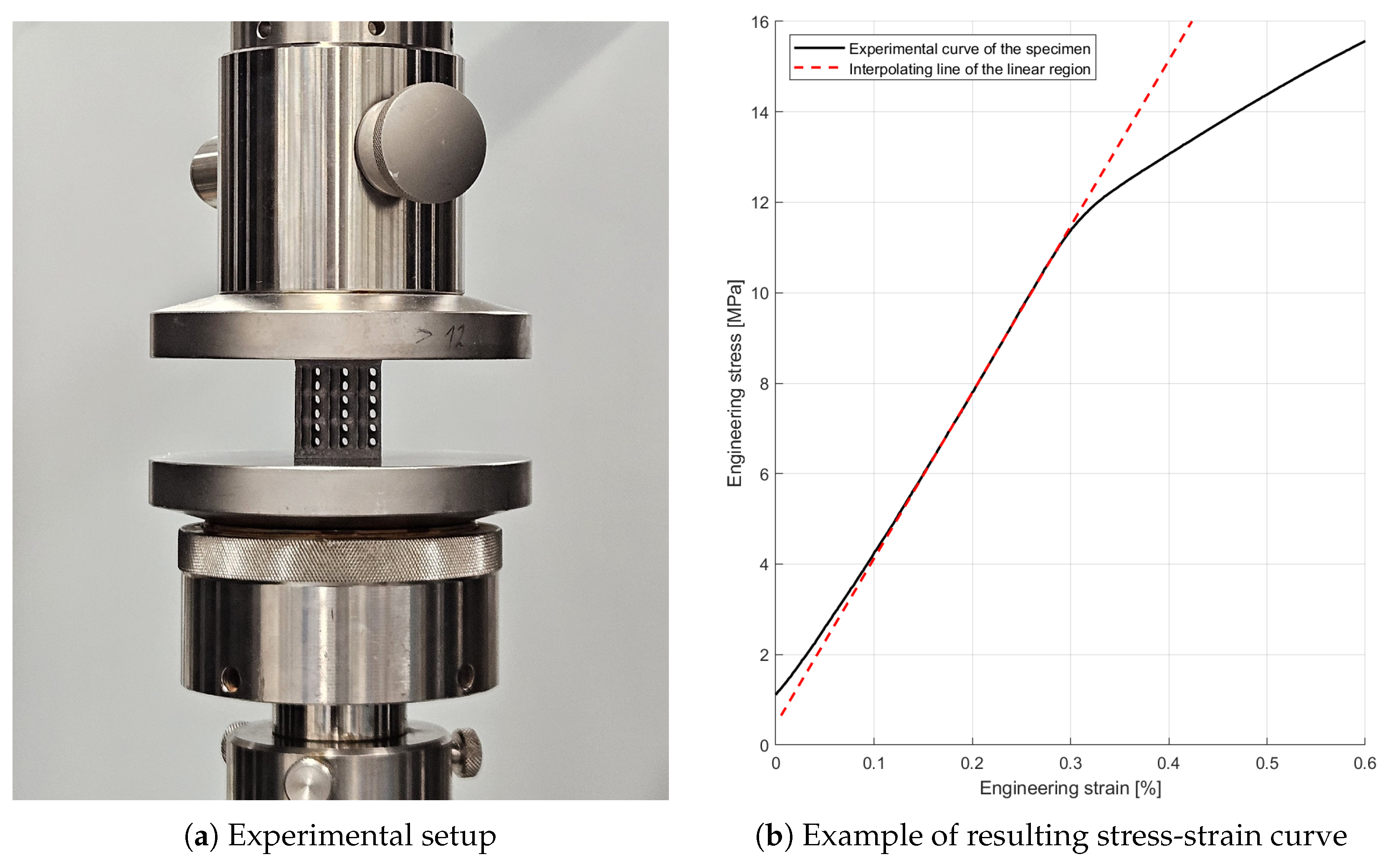
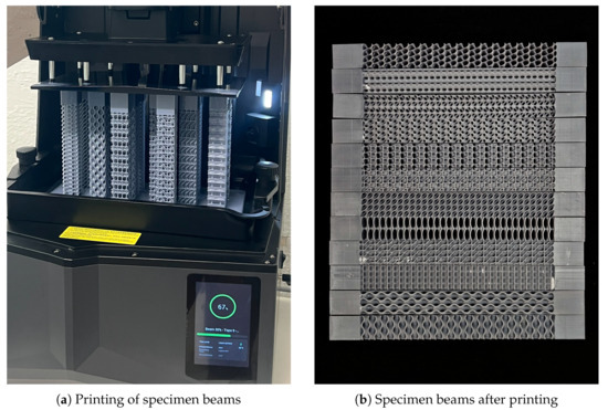
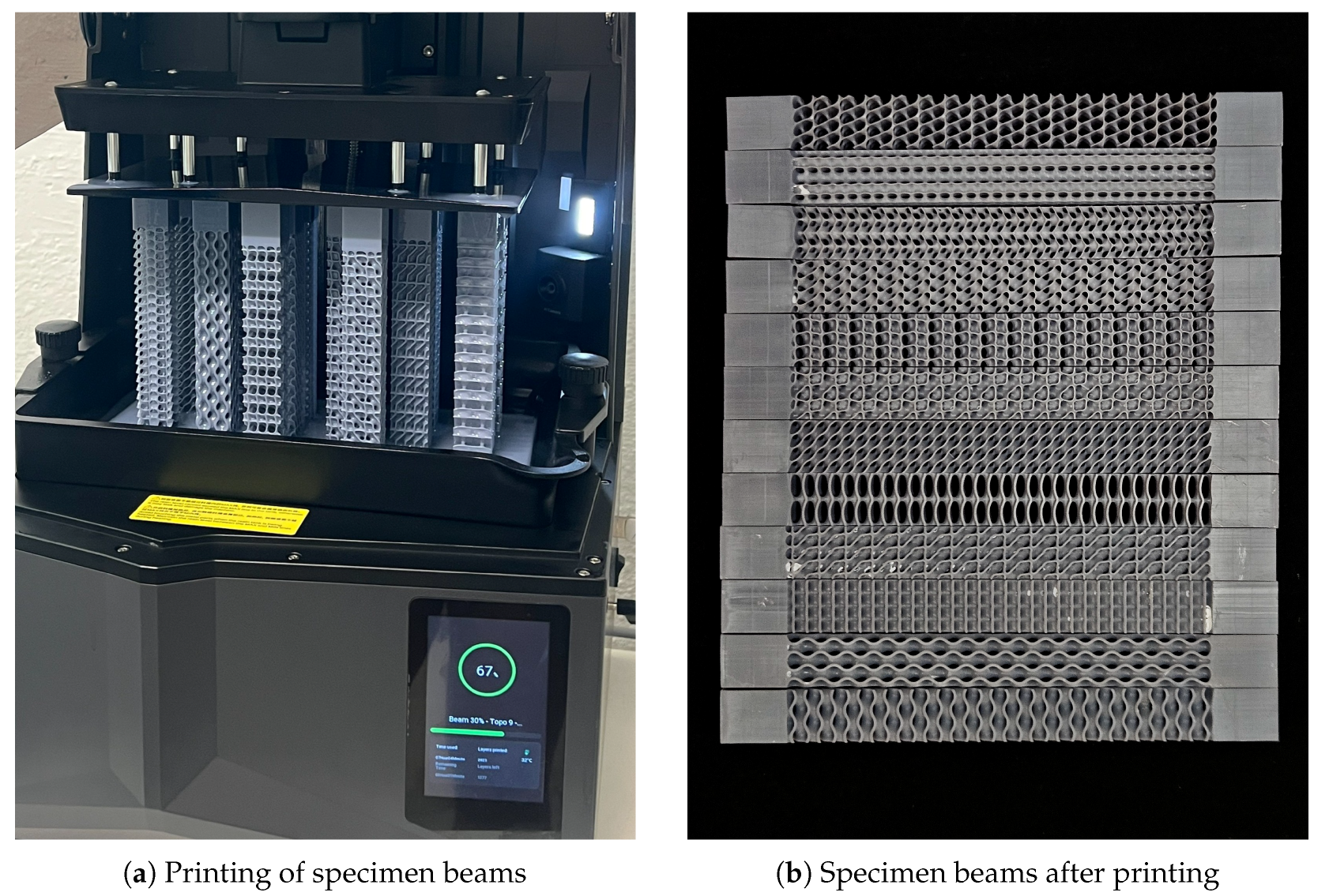
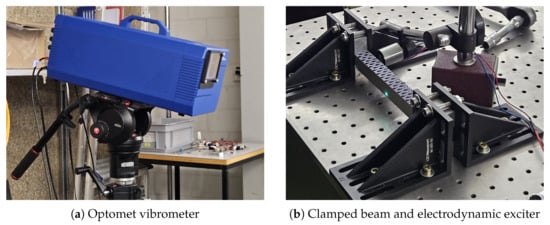
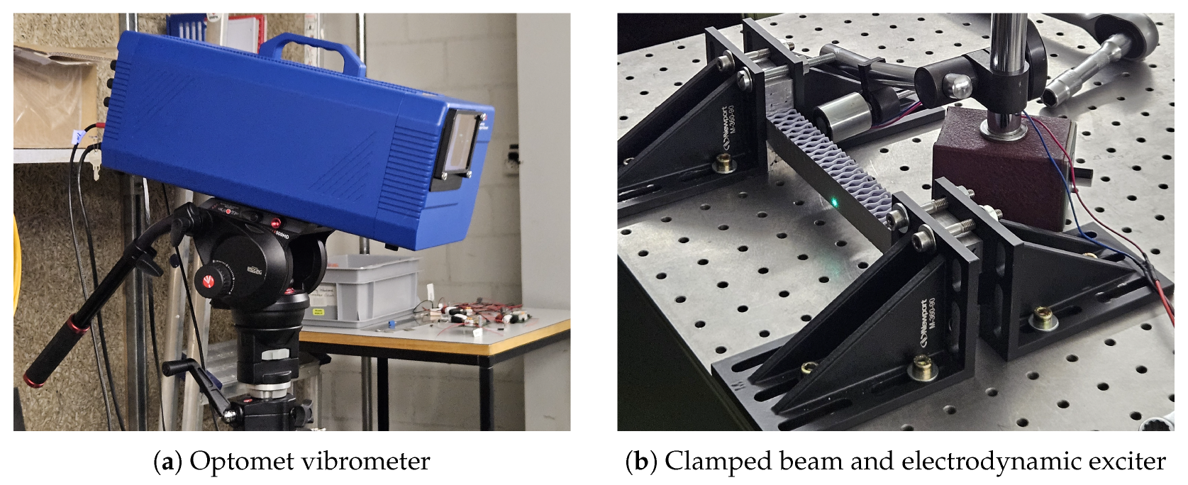

Disclaimer/Publisher’s Note: The statements, opinions and data contained in all publications are solely those of the individual author(s) and contributor(s) and not of MDPI and/or the editor(s). MDPI and/or the editor(s) disclaim responsibility for any injury to people or property resulting from any ideas, methods, instructions or products referred to in the content. |
© 2026 by the authors. Licensee MDPI, Basel, Switzerland. This article is an open access article distributed under the terms and conditions of the Creative Commons Attribution (CC BY) license.