Numerical Investigation of Confined Flow Around Circular and Square Obstacle Using the Multiple Relaxation Time Lattice Boltzmann

Abstract

Flow behavior can be changed by parameters such as fluid properties, geometry, and operating conditions. This paper presents a 2D numerical analysis of incompressible fluid flow in a channel with either a circular or square cylinder using the multiple relaxation time Lattice Boltzmann method (LBM-MRT). All simulations are performed at a fixed Reynolds number of Re = 100. A parabolic velocity profile is imposed at the inlet, while no-slip boundary conditions are adopted at the channel walls and obstacle surfaces. The numerical model is validated by comparing the mean drag coefficient with findings in the literature. Subsequently, the effects of obstacle shape, size, and position on the flow behavior and hydrodynamic forces are investigated. The effects of three obstacle sizes and three distinct positions are investigated for circular and square geometries under identical flow conditions. The results show that increasing the obstacle size modifies the flow and wake structure, and affects the drag and lift coefficients. Compared with the circular obstacle, the square obstacle creates stronger flow disturbances because of its sharp corners. The results also highlight the important effects of obstacle shape, size, and position on the flow characteristics and hydrodynamic coefficients.

1. Introduction

Flow around obstacles confined in a channel is encountered in many engineering and industrial applications, including heat exchangers, pipelines, aerodynamic design, and flow control systems. Obstacles can significantly modify the flow structure, leading to vortex shedding, recirculation zones, and flow separation. Those phenomena directly affect hydrodynamic forces, particularly the drag and lift coefficients. Their characteristics depend on several factors, including the obstacle geometry, size, position, and flow conditions. Therefore, understanding how these parameters influence the flow is essential for accurately predicting and controlling confined flows.

Such flows have traditionally been simulated using computational fluid dynamics (CFD) methods, including the finite difference method (FDM), finite volume method (FVM), and finite element method (FEM). Although these approaches have been successfully applied to a wide range of fluid flow problems, their implementation becomes computationally demanding for complex geometries and unsteady flows due to the challenges associated with mesh generation and pressure–velocity coupling.

The Lattice Boltzmann method (LBM) has emerged as a powerful alternative to conventional CFD methods for simulating fluid flow and transport phenomena. The Lattice Boltzmann method has become a potent substitute for standard numerical techniques in simulating single-phase [1] and multiphase flows [2], as well as transport processes [3]. Unlike traditional CFD approaches that directly solve the Navier–Stokes equations, the LBM is based on the Boltzmann equation and describes fluid motion at a mesoscopic scale [4]. Due to its simple algorithm, efficient parallelization, and capability to handle complex geometries, it has become increasingly appealing for simulating single-phase and multiphase flows, as well as flows around obstacles.

The Lattice Boltzmann Method (LBM) evolved from the lattice–gas automata (LGA) approach, and has subsequently become an established numerical framework for simulating fluid flows. Recent reviews have highlighted its development from LGA to modern LBM formulations, and its applications to nearly incompressible flows [5,6].

This innovative method has gained widespread recognition within the scientific community for modeling intricate fluid dynamics, as introduced by McNamara and Zanetti [5] in 1988. Since then, LBM has been widely used by researchers for modeling incompressible flows with intricate geometries and moving boundaries, and for flow around obstacles [7,8], and it has been proven to have greater capability and fluidity compared to traditional CFD techniques.

Several collision models have been developed within the LBM framework. The BGK model, the most basic relaxation time approach, is widely employed [9]. However, its numerical stability and accuracy may be limited for complex flows involving strong velocity gradients and flow separation. D’Humières [10] introduced the MRT model to address these limitations.

This feature greatly improves numerical stability and offers more control over dissipative processes. Lallemand and Luo [11] claim that the MRT model enhances the accuracy of different flow configurations and reduces non-physical oscillations. Moreover, improved numerical performance and decreased dispersion errors result from the conversion of the collision process into moment space [12].

The LBM, and particularly its MRT formulation, has been widely used to investigate flows around bluff bodies such as circular and square cylinders, and becomes particularly evident in flows characterized by moderate to high Reynolds numbers and strong gradients, such as separation regions, vortex shedding, and recirculation zones [13,14].

Wu et al. [15] applied the LBM-MRT to the flow past a square cylinder at Re = 100, and demonstrated its ability to predict the periodic vortex-shedding regime and associated hydrodynamic coefficients. Filip et al. [16] compared different collision models (BGK, TRT, and MRT) for confined cylinder flows, and reported improved accuracy for the MRT scheme.

Similarly, Grucelski et al. [8] investigated the hydrodynamic and thermal behavior of flow around a circular cylinder, highlighting the importance of wake development.

Li et al. [17] compared the MRT and BGK (SRT) models for flow around a circular cylinder and showed the improved stability and accuracy of the MRT approach. Other studies have also investigated the influence of Reynolds number on wake formation and vortex shedding behind circular cylinders [18].

Recent studies have further highlighted the sensitivity of bluff body flows to obstacle geometry and confinement. Fezai et al. [19] investigated flow around square cylinders with different staggered arrangements, and showed that the obstacle configuration strongly affects the wake structures, drag and lift forces, and vortex-shedding behavior. Ali et al. [20] used the Lattice Boltzmann Method (LBM) to study how fluid moves around a square cylinder. They found that changing the shape of the cylinder leads to changes in the forces that the fluid applies, and in the swirling patterns of the flow. In a related study, Ali et al. [21] demonstrated that the spacing between square cylinders can substantially modify wake interactions, vortex shedding, and the corresponding drag and lift coefficients. For circular cylinders, Nguyen and Lei [22] examined the effect of blockage on hydrodynamic characteristics and showed that increasing confinement can significantly increase the mean drag coefficient and Strouhal number, while also modifying the wake dynamics. Similarly, recent numerical studies of confined circular-cylinder flows have reported great changes in wake asymmetry and vortex organization with variations in Reynolds number and blockage ratio [23]. More recently, Granados-Ortiz et al. [24] used the LBM to investigate both circular and square cylinder flows at (Re = 100), demonstrating that the method can reproduce the characteristic oscillatory wake and hydrodynamic coefficients for confined configurations. These studies demonstrate that wake development and hydrodynamic forces are strongly influenced by the interaction between obstacle geometry, confinement, and flow conditions. However, the literature remains fragmented, as most studies focus on either circular or square obstacles and generally vary one parameter at a time, such as Reynolds number, blockage ratio, or obstacle arrangement. In particular, systematic comparisons between circular and square obstacles with different sizes and streamwise positions under identical confined-flow conditions remain limited. This study addresses this gap by examining the combined effects of obstacle shape, size, and streamwise position at a fixed Reynolds number (Re = 100), with emphasis on wake development, vortex shedding, and drag and lift coefficients.

The literature remains fragmented, as most studies focus on either circular or square obstacles and generally vary one parameter at a time.

This previous research provides valuable information about the numerical performance of the LBM and the flow characteristics around individual bluff obstacles. However, most studies focus on a single obstacle geometry, a specific obstacle position, or the influence of geometric parameters. Consequently, a systematic assessment of circular and square obstacles with identical parameters under the same confined flow conditions is needed. In particular, the combined influence of obstacle shape, size, and position on wake development and hydrodynamic forces is examined.

In this regard, the main novelty of the current work is a systematic comparison of circular and square obstacles under identical confinement and flow conditions. Three obstacle sizes and three streamwise positions are considered for both geometries at a fixed Reynolds number (Re = 100). This approach makes it possible to isolate and compare the effect of obstacle shape, size, and position on the flow structure, wake development, vortex shedding, and hydrodynamic forces. The flow fields are analyzed using velocity contours, streamlines, and velocity distributions, while the drag and lift coefficients and vortex shedding characteristics are evaluated.

The remainder of this paper is organized as follows. Section 2 presents the physical problem, and the governing equations and the numerical method based on the LBM-MRT model are described. Section 3 is devoted to the results and discussion. Finally, conclusions and future perspectives are provided in the last section.

2. Materials and Methods

2.1. Physical Problem and Mathematical Formulation

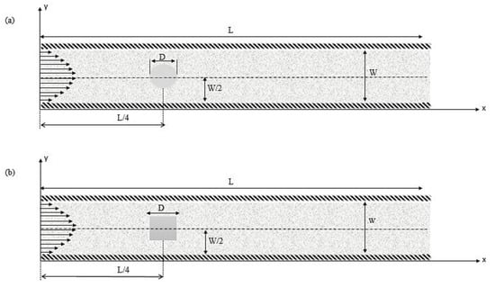
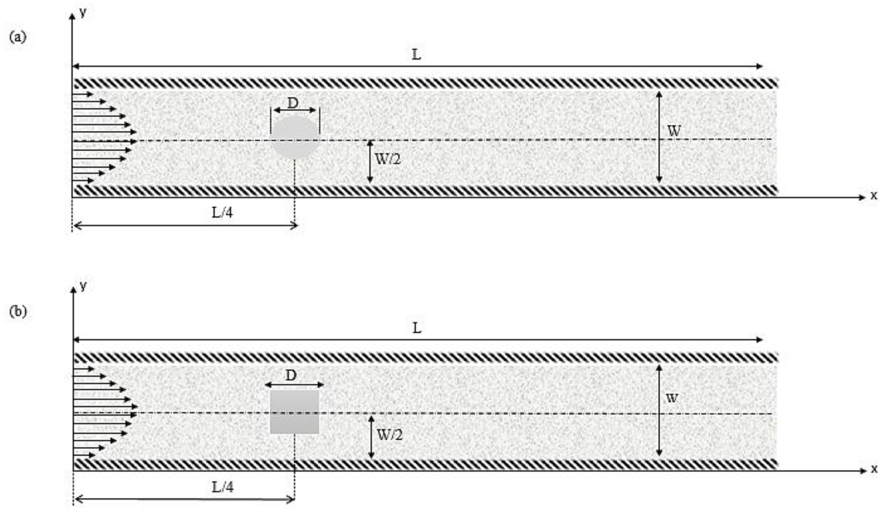
The physical problem is illustrated in Figure 1. The channel has a length L and a height W. The obstacle, with hydraulic diameter D, is at the centerline of the channel and is located at a distance H from the entrance of the channel. The fluid enters with a parabolic velocity profile. No-slip boundary conditions are adopted at the walls. The fluid used is air, and it is considered Newtonian and incompressible. The Reynolds number (Re) is the ratio of inertial forces to viscous forces, and the flow is assumed to be laminar and incompressible.

Figure 1. Schematic diagram of fluid flow domain around an obstacle: (a) circular obstacle; (b) square obstacle. The light gray region represents the fluid domain, the darker gray region indicates the obstacle, and the hatched borders represent the solid channel walls.

The channel with circular and square obstacles is depicted in Figure 1a,b.

The boundary conditions applied in this study include no-slip conditions on both the channel and the obstacles walls. At the inlet and outlet, appropriate boundary conditions are imposed on the left and right sides of the channel, respectively.

The boundary conditions for this case are

$$\left\{\begin{array}{c}\mathrm{x}=0:\mathrm{u}=u_{in},\mathrm{v}=0\\ x=L:{\displaystyle \frac{\partial \mathrm{u}}{\partial X}}={\displaystyle \frac{\partial \mathrm{v}}{\partial X}}=0\\ \mathrm{Y}=0 \mathrm{a}\mathrm{n}\mathrm{d} \mathrm{Y}=\mathrm{W}:\mathrm{u}=\mathrm{v}=0\end{array}\right.$$

The flow is governed by the conservation equations of mass and momentum in dimensionless form, as follows:

$${\displaystyle \frac{\partial u}{\partial x}}+{\displaystyle \frac{\partial v}{\partial y}}=0$$

(1)

The momentum equations are given by

$$\left(u{\displaystyle \frac{\mathit{\text{∂}}u}{\mathit{\text{∂}}x}}+v{\displaystyle \frac{\mathit{\text{∂}}u}{\mathit{\text{∂}}y}}\right)=-{\displaystyle \frac{\mathit{\text{∂}}P}{\mathit{\text{∂}}x}}+{\displaystyle \frac{1}{R_e}}\left({\displaystyle \frac{{\mathit{\text{∂}}}^{2}u}{\mathit{\text{∂}}{x}^2}}+{\displaystyle \frac{{\mathit{\text{∂}}}^{2}u}{\mathit{\text{∂}}{y}^2}}\right)$$

(2)

$$\left(u{\displaystyle \frac{\mathit{\text{∂}}v}{\mathit{\text{∂}}x}}+v{\displaystyle \frac{\mathit{\text{∂}}v}{\mathit{\text{∂}}y}}\right)=-{\displaystyle \frac{\mathit{\text{∂}}P}{\mathit{\text{∂}}y}}+{\displaystyle \frac{1}{R_e}}\left({\displaystyle \frac{{\mathit{\text{∂}}}^{2}v}{\mathit{\text{∂}}{x}^2}}+{\displaystyle \frac{{\mathit{\text{∂}}}^{2}v}{\mathit{\text{∂}}{y}^2}}\right)$$

(3)

where $u$ and $v$ are the dimensionless components of the velocity field, P is the pressure, and Re is the Reynolds number [4,24].

The velocity (u) and cylinder diameter (D) determine the flow’s Reynolds number.

$$R_e={\displaystyle \frac{uD}{\vartheta }}$$

(4)

Here, $\vartheta$ is the kinematic viscosity of the fluid.

2.2. Numerical Resolution Method

2.2.1. Lattice Boltzmann Method

The general form of the Lattice Boltzmann equation can be expressed as follows [13]:

$$f_i\left(x+c_{\mathit{i}}∆t,t+∆t\right)-f_i\left(x,t\right)=-{\displaystyle \frac{1}{\tau }}\left(f_i\left(x,t\right)-f_i^{eq}\left(x,t\right)\right)$$

(5)

Here, $f_i(\mathbf{x},t)$ denotes the particle distribution function in the direction $i$ at position $\mathbf{x}$ and time $t$, ${\mathbf{c}}_i$ represents the discrete lattice velocity, $f_i^{eq}$ is the corresponding equilibrium distribution function, and $\tau$ is the relaxation time related to the fluid viscosity.

$f_i^{eq}$ is the equilibrium distribution function, which can be expressed as

$$f_i\left(x+c_i∆t,t+∆t\right)-f_i\left(x,t\right)=-{\displaystyle \frac{1}{\tau }}\left(f_i\left(x,t\right)-f_i^{eq}\left(x,t\right)\right)$$

(6)

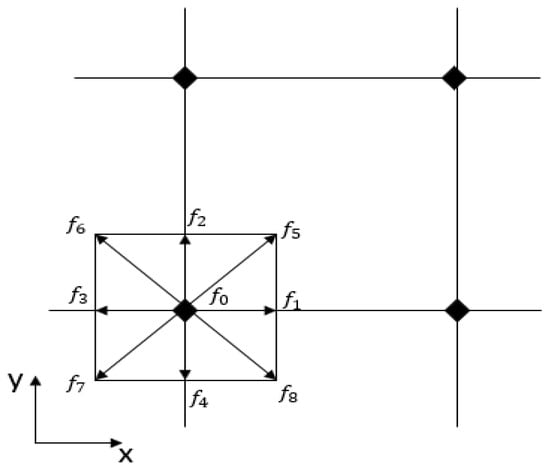
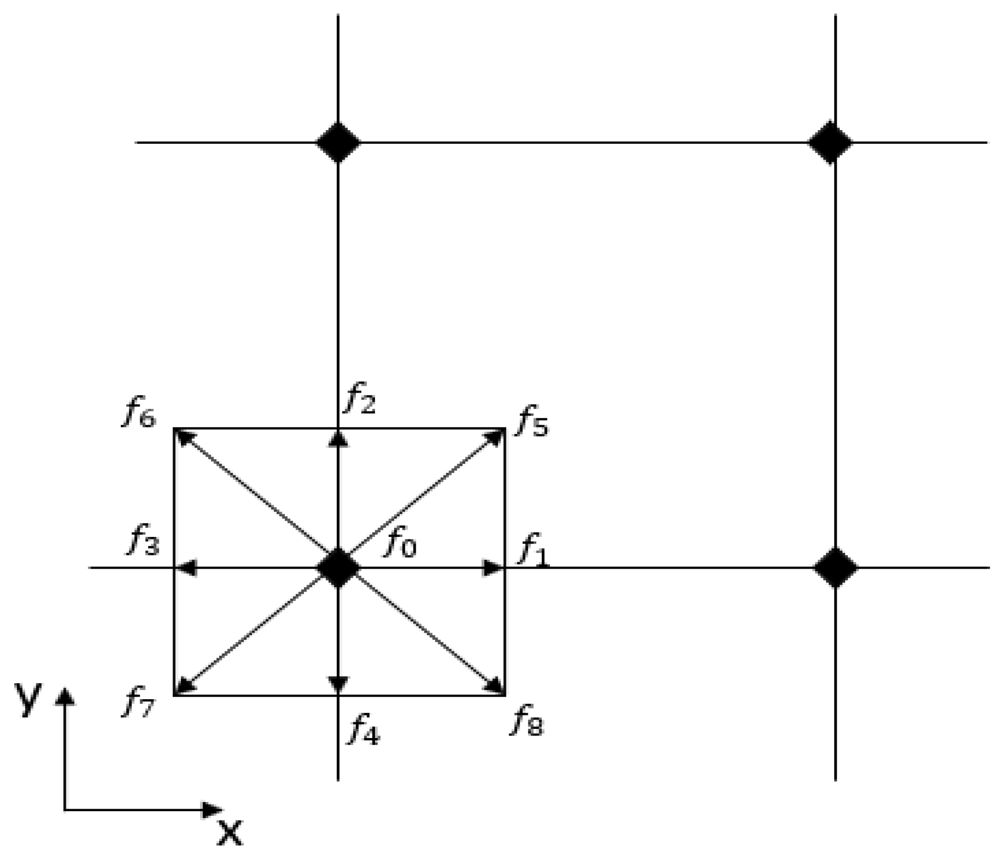
Depending on the geometry of the problem, several models can be employed in LBM; however, the D2Q9 model is chosen for this study [25], as illustrated in Figure 2.

Figure 2. Schematic of the D2Q9 model.

The distribution function is used to derive the macroscopic fluid variables, density $\rho$ and velocity $U$, as follows:

$$\rho (x,t)={\sum }_{i}fᵢ\left(x,t\right)$$

(7)

$$u(x,t)={\displaystyle \frac{1}{\rho }}{\sum }_i{c}_{i}fᵢ(x,t)$$

(8)

In this work, the LBM-MRT model is adopted. The collision procedure is carried out in the moment space as follows:

$${\mathit{\Omega }}_i=-{\mathit{M}}^{-1}\mathit{S}\left(m_i\left(x,t\right)-{m_i}^{eq}\left(x,t\right)\right)$$

(9)

Here, $m_i\left(x,t\right)$ and ${m_i}^{eq}$ are, respectively, the moments and equilibrium moments at the direction I, with

$$m_i(x,t)=\mathit{M}{f}_i(x,t)$$

(10)

where the transformation matrix M and the inverse transformation matrix M⁻¹ are respectively written as [15,26]

$$M=\left[\begin{array}{ccccccccc}1& 1& 1& 1& 1& 1& 1& 1& 1\\ -4& -1& -1& -1& -1& 2& 2& 2& 2\\ 4& -2& -2& -2& -2& 1& 1& 1& 1\\ 0& 1& 0& -1& 0& 1& -1& -1& 1\\ 0& -2& 0& 2& 0& 1& -1& -1& 1\\ 0& 0& 1& 0& -1& 1& 1& -1& -1\\ 0& 0& -2& 0& 2& 1& 1& -1& -1\\ 0& 1& -1& 1& -1& 0& 0& 0& 0\\ 0& 0& 0& 0& 0& 1& -1& 1& -1\end{array}\right]$$

(11)

$$M^{-1}=a\left[\begin{array}{ccccccccc}4& -4& 4& 6& 0& 0& 0& 0& 0\\ 4& -1& -2& 6& -6& 0& 0& 9& 0\\ 4& -1& -2& 0& 0& 6& -6& -9& 0\\ 4& -1& -2& -6& 6& 0& 0& 9& 0\\ 4& -1& -2& 0& 0& -6& 6& -9& 0\\ 4& 2& 1& 6& 3& 6& 3& 0& 9\\ 4& 2& 1& -6& -3& 6& 3& 0& -9\\ 4& 2& 1& -6& -3& -6& -3& 0& 9\\ 4& 2& 1& 6& 3& -6& -3& 0& -9\end{array}\right]$$

(12)

where $a=1/36$.

Therefore, the discrete Boltzmann equation (5) has been modified, and can be written for this model as follows:

$$f_i\left(x+c_i∆t,t+∆t\right)-f_i\left(x,t\right)=-M^{-1}S\left(m_i\left(x,t\right)-m_i^{eq}\left(x,t\right)\right)$$

(13)

The relaxation matrix S is a diagonal matrix expressed as

$$S=\left[\begin{array}{ccc}\begin{array}{ccc}{s}_0& 0& 0\\ 0& s_1& 0\\ 0& 0& s_2\end{array}& \begin{array}{ccc}0& 0& 0\\ 0& 0& 0\\ 0& 0& 0\end{array}& \begin{array}{ccc}0& 0& 0\\ 0& 0& 0\\ 0& 0& 0\end{array}\\ \begin{array}{ccc}0& 0& 0\\ 0& 0& 0\\ 0& 0& 0\end{array}& \begin{array}{ccc}{s}_3& 0& 0\\ 0& s_4& 0\\ 0& 0& s_5\end{array}& \begin{array}{ccc}0& 0& 0\\ 0& 0& 0\\ 0& 0& 0\end{array}\\ \begin{array}{ccc}0& 0& 0\\ 0& 0& 0\\ 0& 0& 0\end{array}& \begin{array}{ccc}0& 0& 0\\ 0& 0& 0\\ 0& 0& 0\end{array}& \begin{array}{ccc}{s}_6& 0& 0\\ 0& s_7& 0\\ 0& 0& s_8\end{array}\end{array}\right]$$

(14)

$S$ can be expressed as follows:

$$S=diag\left(\mathrm{1.0,1.4,1.4},s_3,1.2,s_5,1.2,s_7,s_8\right)$$

(15)

where $s_7=s_8=2/(1+6\vartheta )$, $s_3$and $s_5$ are arbitrary, and can be set to 1.0.

The evolution Equation (12) is composed of two [12] steps,

$$\mathrm{Collision}:f_i^{\ast }=f_i-M^{-1}S\left(m_i-{m_i}^{eq}\right)$$

(16)

$$\mathrm{Streaming}:f_i\left(x+c_{\mathit{i}}∆t,t+∆t\right)=f_i^{\ast }\left(x,t\right)$$

(17)

Here, $f_i^{\ast }$ is the distribution function after collision.

The equilibrium moments are calculated as follows:

$$m_0^{eq}=\rho$$

(18)

$$m_1^{eq}=\rho \left[-2+3\rho \left(u_x^2+u\right)\right]$$

(19)

$$m_2^{eq}=\rho \left[1-3\rho \left(u_x^2+u_y^2\right)\right]$$

(20)

$$m_3^{eq}=\rho u_x$$

(21)

$$m_4^{eq}=-\rho u_x$$

(22)

$$m_5^{eq}=\rho u_y$$

(23)

$$m_6^{eq}=-\rho u_y$$

(24)

$$m_7^{eq}={\rho }^2\left(u_x^2-u_y^2\right)$$

(25)

$$m_8^{eq}={\rho }^2{u}_x{u}_y$$

(26)

2.2.2. Boundary Conditions

Boundary conditions play a key role in ensuring the accuracy and stability of numerical simulations. Poorly implemented boundary conditions may lead to significant errors or numerical instabilities. In the Lattice Boltzmann Method (LBM), boundary conditions are applied to particle distribution functions rather than macroscopic variables. Therefore, the proper implementation of these conditions is essential for obtaining reliable and physically consistent results.

For no-slip walls, the non-equilibrium distribution function bounce-back approach established by Zou and He [8] is employed. In the bounce-back boundary condition, particle distribution functions are reflected along their incoming direction after colliding with the wall. Unknown distribution functions at the wall and pointing into the fluid domain are calculated as follows.

At inlet (X = 0),

$${\rho }_0={\displaystyle \frac{1}{{1-u}_0}}\left(f_0+f_2+f_4+2\left(f_3+f_7+f_8\right)\right)$$

(27)

$$f_1=f_3+{\displaystyle \frac{2}{3}}{\rho }_0{u}_0$$

(28)

$$f_5=f_7-{\displaystyle \frac{1}{2}}\left(f_2-f_4\right)+{\displaystyle \frac{1}{6}}\rho u_0$$

(29)

$$f_8=f_6+{\displaystyle \frac{1}{2}}\left(f_2-f_4\right)+{\displaystyle \frac{1}{6}}{\rho }_0{u}_0$$

(30)

For outlet boundary (X = 1), it is expressed as below:

$$f_3=f_1-{\displaystyle \frac{2}{3}}\rho u_0$$

(31)

$$f_7=f_5+{\displaystyle \frac{1}{2}}\left(f_2-f_4\right)-{\displaystyle \frac{1}{6}}\rho u_0$$

(32)

$$f_6=f_8-{\displaystyle \frac{1}{2}}\left(f_2-f_4\right)-{\displaystyle \frac{1}{6}}\rho u_0$$

(33)

In the present LBM simulation, the momentum exchange method is used to compute the fluid force on the circular cylinder. The total force exerted on a solid body by the fluid can be written as [27]

$$F={\sum }_{x_f}{\sum }_{{i\in \mathrm{\Omega }}_b}\left[f_i^{\ast }\left(x_b,t\right)+f_{\overline{i}}^{\ast }{f}_{\overline{i}}\left(x_f,t\right)\right]c_i$$

(34)

where $f_i^{\ast }$ is the post-collision distribution function.

Lift and drag coefficients are calculated as follows:

Drag coefficient—

$$C_D={\displaystyle \frac{F_D}{\frac{1}{2}\rho u^{2}D}}$$

(35)

Lift coefficient—

$$C_L={\displaystyle \frac{F_L}{\frac{1}{2}\rho u^{2}D}}$$

(36)

Here, $C_D$ and $C_L$ are drag and lift coefficients; lift and drag forces are denoted by $F_L$ and $F_D$, respectively. The momentum exchange (ME) approach, a popular force-evaluation methodology in LBM, predicts the $F_D$ and $F_L$ [28].

2.2.3. Code Validation and Accuracy of the Numerical Simulation

• Solution procedure

The computational domain for the 2D configuration is defined by the boundaries (0 ≤ x ≤ L, 0 ≤ y ≤ W) and is divided into a uniform grid with equal spacing (∆_xx = ∆_yx = 0.001 m), resulting in a total of (N_x × N_y = 1500 × 320) lattice nodes. The corresponding physical dimensions of the computational domain are therefore (Lx = 1.5 m) and (Wx = 0.32 m). The obstacle size is initially specified in lattice units (LU), and the corresponding physical dimension is obtained using $D_{physique}=D_{LU}{∆}_x$. Accordingly, obstacle sizes of (Dx = 10), (Dx = 20) and (Dx = 30) LU correspond to physical dimensions of (0.01), (0.02), and (0.03) m, respectively. The obstacle is positioned at L/4, L/2, and 3L/4 along the channel. The Reynolds number is defined based on the obstacle height and the inlet velocity. A parabolic velocity profile is imposed at the channel inlet, a zero-momentum flux condition is applied at the outlet, and non-slip boundary conditions are enforced at both the walls and the obstacle.

To investigate the effect of obstacle shape, size, and position under comparable flow conditions, the Reynolds number based on the characteristic obstacle dimension was held constant at Re = 100. As the obstacle was varied, the kinematic viscosity was adjusted accordingly to satisfy $R_e={\displaystyle \frac{uD}{\vartheta }}$. The corresponding blockage ratios (D/W) and simulation parameters for all cases are summarized in Table 1.

Table 1. Numerical and physical parameters of the LBM simulation.

Obstacle Shape	Streamwise Position	Obstacle Size (LU)	D/W
	L/4	D = 20	0.0625
Circular	L/2	D = 40	0.125
	3L/4	D = 60	0.1875
	L/4	D = 20	0.0625
Square	L/2	D = 40	0.125
	3L/4	D = 60	0.1875

To perform Lattice Boltzmann Method (LBM) computations, a two-dimensional numerical code has been developed in Fortran. The algorithm is as follows: the $f_i$ are transformed into moments $m_i$ via the transformation matrix $M$, the collision is carried out in moment space through the relaxation matrix S, then $m_i$ are transformed back to $f_i$ via the inverse transformation matrix $M^{-1}$. The algorithmic steps are outlined as follows:

Firstly, give the simulation parameters and initialize the distribution functions and macroscopic variables.

• Calculate moments and equilibrium moments;
• Provide the collision step, and then calculate post-collision distribution functions using the M⁻¹ transformation;
• Introduce boundary conditions;
• Provide the streaming process and calculate macroscopic variables;
• Check convergence and repeat from step 2 if the convergence criteria are not verified.

• Validation

To ensure the accuracy of the results and validate the simulation code, flow around circular and square cylinders in an open channel is considered. The Drag coefficient C_D is calculated, and the results are compared with those of previous studies [29,30,31,32,33,34] and gathered in Table 2.

Table 2. Comparison of Drag coefficient (C_D) values at a Reynolds Number of 100.

Authors	CD circular	CD  square
Present	1.256	----- *
Braza et al. [29]	1.364	----- *
Calhoun [30]	1.330	----- *
PD Arumuga et al. [31]	1.290	----- *
Present	----- *	1.507
M.Breuer et al. [32]	----- *	1.34
AK.Sahu et al. [33]	----- *	1.42
Y.Zhou et al. [34]	----- *	1.443

* The corresponding geometry is not exist in the related reference.

As can be seen from Table 2, the present results show good agreement with those from the literature.

3. Results

In this Section, the details of flow patterns, the drag (C_D) and lift (C_L) coefficients around circular and square cylinders, will be mainly discussed, which reveal some variation under the given conditions.

3.1. Effect of Cylinder Position

This section explores the influence of obstacle position on the flow structure and hydrodynamic behavior. Along the channel, three distinct streamwise locations are consideration.

For a fixed blockage ratio and Reynolds number, only the confinement and the obstacle position govern the flow regime. The obstacle is placed at three different streamwise locations (L/4, L/2, and 3L/4) within the channel, as shown in Figure 3 and Figure 4, in order to investigate its influence on the velocity field distribution.

Figure 3. Velocity distribution for different positions of the circular obstruction: (a) Upstream obstacle position L/4, (b) central obstacle position L/2, and (c) downstream obstacle position 3L/4.

Figure 4. Velocity distribution for different positions of the square obstruction: (a) Upstream obstacle position L/4, (b) central obstacle position L/2, and (c) downstream obstacle position 3L/4.

The streamwise position of the cylinders influences the wake structure and vortex shedding behavior.

As described in Figure 3a, for the first case located at L/4, a long and well-developed wake forms downstream of the obstacle, characterized by alternating vortical structures. In this configuration, a Karman vortex street develops, resulting from periodic flow separation on both sides of the obstacle. When the obstacle is shifted to the L/2 position as shown in Figure 3b, the shorter downstream region limits the development of the vortical structures, although they are still apparent. For the Theard position at 3L/4, Figure 3c shows that the wake becomes shorter and more compact, with less developed vortical structures before the outflow.

As shown in Figure 4a for the first position (L/4) with the square obstacle, one can clearly see that the flow separates sharply at the upstream and downstream corners of the obstacle, generating a low-velocity region and a well-developed wake. This behavior indicates the formation of a Karman vortex street, resulting from periodic vortex shedding.

Compared to the obstacle position in the flow structure, it can be seen that when the obstacle is located far from the outflow of the channel (at L/4), a long and well-developed wake is formed downstream, and the wake is more developed and becomes progressively shorter as the obstacle moves toward the outflow (at 3L/4), creating a more abrupt flow separation because of the sharp corners of the square geometry.

Overall, moving the obstacle toward the outlet progressively reduces the available wake-development region and modifies the recirculation and vortex structures downstream of the obstacle.

3.2. Effect of Cylinder Diameter on Flow

This subsection discusses the flow patterns around circular and square cylinders of sizes D = 20 LU, 40 LU, and 60 LU, placed at three streamwise positions, L/4, L/2, and 3L/4, respectively. The flow around two cylinder shapes is sensitive to both size and position.

3.2.1. Circular Shape

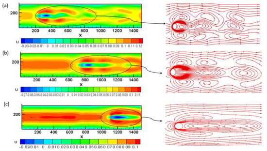
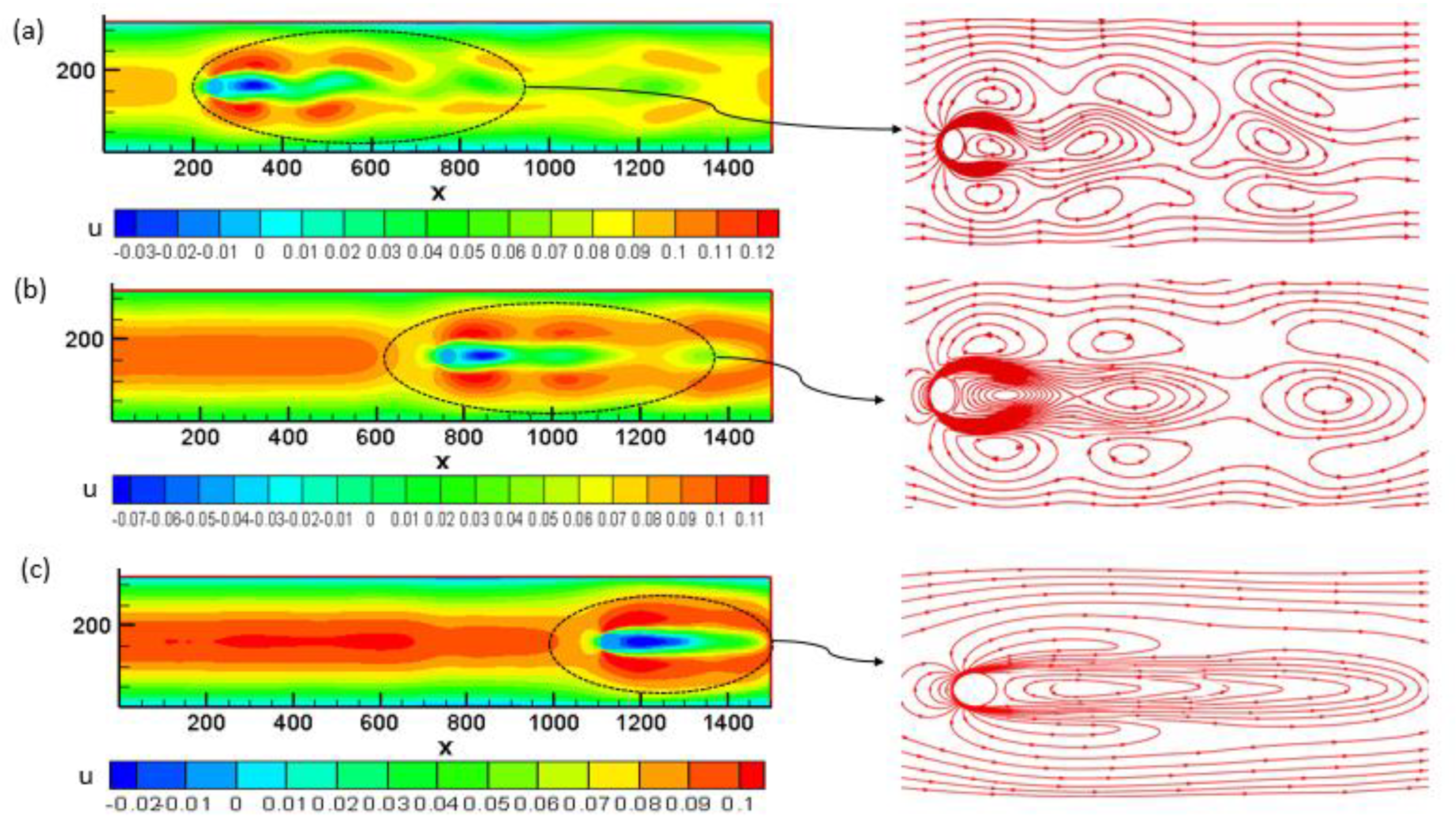
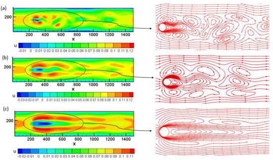
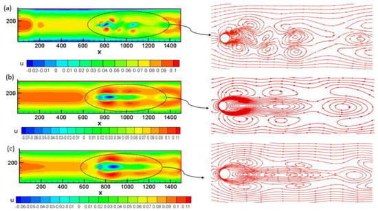
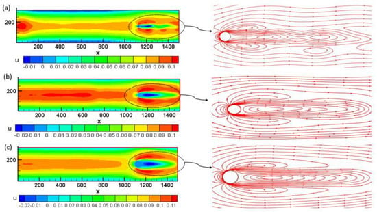
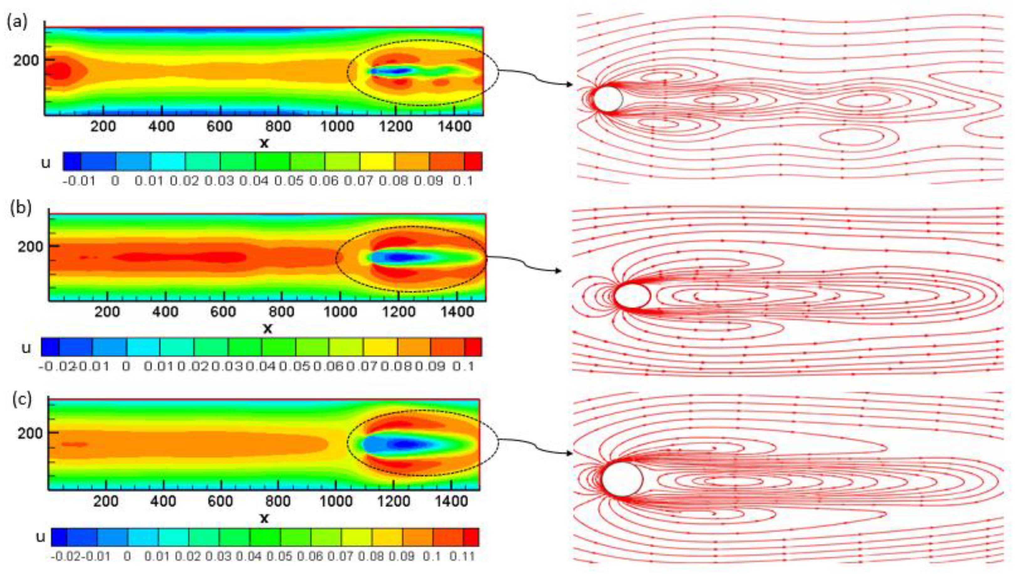
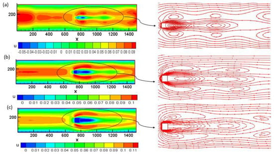
The flow around a circular obstacle is sensitive to its size (D) and position. To demonstrate the effect of obstacle size on the flow field, the corresponding vorticity field and streamlines are shown in Figure 5, Figure 6 and Figure 7.

Figure 5. Velocity distributions for different−sized circular obstacles at the Upstream obstacle position L/4: (a) D = 20, (b) D = 40, and (c) D = 60.

Figure 6. Velocity distributions for different−sized circular obstacles at the Central obstacle position L/2: (a) D = 20, (b) D = 40, and (c) D = 60.

Figure 7. Velocity distributions for different−sized circular obstacles at the Downstream obstacle position 3L/4: (a) D = 20, (b) D = 40, and (c) D = 60.

Figure 5a–c depict the flow patterns at the L/4 position. As shown in Figure 5a for D = 20 LU, the obstacle’s size is too small to strongly influence the weak, producing a relatively weak disturbance, with a narrow wake and a limited recirculation region downstream. The flow exhibits a large characteristic length, and it should be noted that a vortex street forms downstream.

As depicted in Figure 5b, when the diameter increases to D = 40 LU, it can be seen that the confinement effects become dominant, the disturbance becomes more pronounced, and the flow acceleration is more marked around the obstacle due to blockage. This leads to a clearer contraction of the effective flow passage, an expansion of the wake region downstream, and an increase in both the size and the intensity of the recirculation zones behind the obstacle.

As illustrated in Figure 5c, increasing the obstacle diameter to D = 60 LU strengthens the confinement effect. It can be seen that the larger cylinder occupies a significant portion of the channel, causing the pronounced acceleration of the fluid around the obstacle, a higher blockage ratio, and steeper velocity gradients. As a result, a broader and more noticeable wake forms downstream, accompanied by a larger recirculation zone and longer-range vortical formations.

Consequently, the increase in obstacle size also affects the vortex-shedding pattern. For D = 20 LU, the wake is relatively narrow, and the vortical structures are less pronounced. As the diameter increases, flow separation is enhanced, promoting the development of larger vortical structures downstream. At D = 60 LU, the wake is therefore more strongly disturbed, and the vortex-shedding region becomes more pronounced.

As shown in Figure 6a, the flow pattern exhibits a localized disturbance around the central obstacle. At the smallest equivalent diameter (D = 20 LU), the perturbation remains confined to the near-wake region, with minimal distortion of the upstream and downstream streamlines, indicating a weak interaction between the flow and the cylindrical element.

As illustrated in Figure 6b,c, for increasing obstacle sizes of D = 40 LU and D = 60 LU, respectively, the flow perturbation and acceleration become more pronounced; the vortices grow more intense and larger, accompanied by an increase in the recirculation area and more pronounced vortex detachment.

Figure 6b,c show that the streamlines are more strongly diverted and compressed around the obstacle, with more pronounced separation and an extended region before flow reattachment.

As illustrated in Figure 7, and as explained in Section 3.1, one can clearly see that, at this specific location, regardless of the cylinder diameter D, moving the obstacle toward the outlet progressively reduces the available wake development region and modifies the recirculation and vortex structures downstream of the obstacle. However, at the present position, no significant variation is observed, indicating that the influence of obstacle size remains strictly confined to the near-wake region and does not extend to this particular location.

Overall, the phenomena described above clearly illustrate that the equivalent diameter D exerts a significant influence on the flow typology. The key effects—namely, flow separation, recirculation, and confinement—progressively intensify with increasing D. This trend underscores the critical role of obstacle size in modulating wake dynamics, mixing characteristics, and aerodynamic loading.

3.2.2. Square Shape

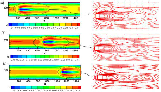
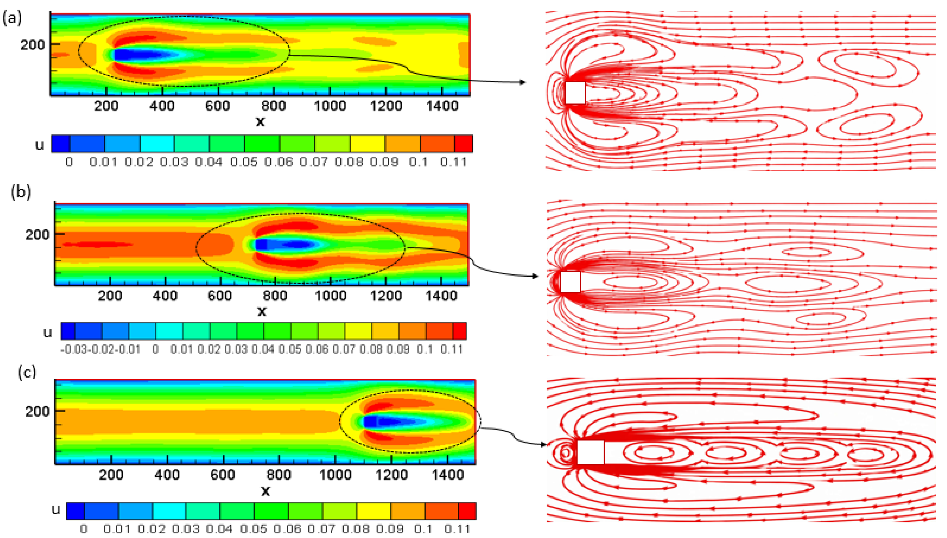
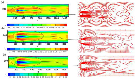
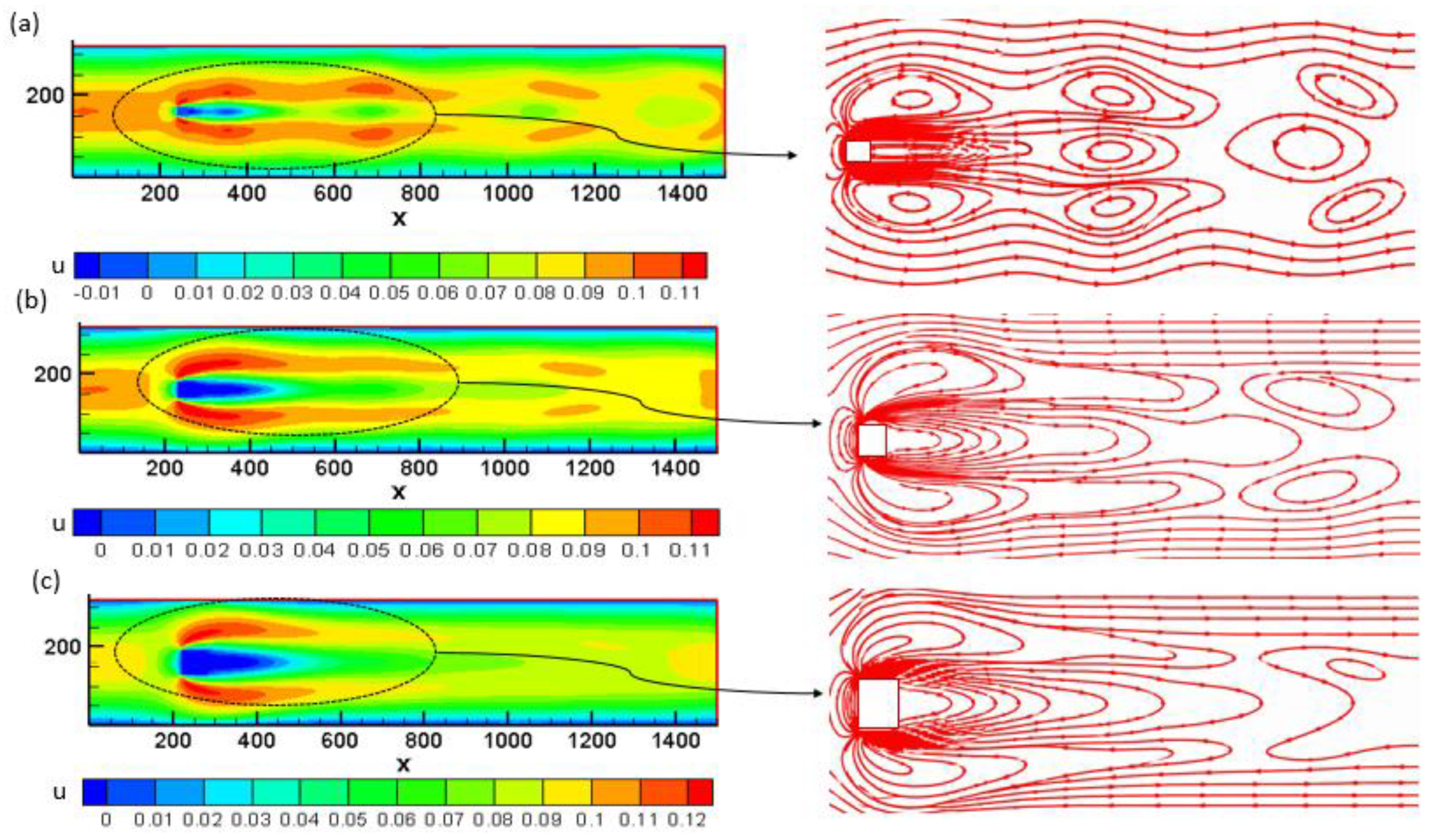
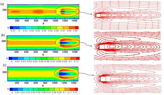
This subsection discusses the flow pattern around the square cylinder and demonstrates the effect of the obstacle size on the overall flow field, as shown in Figure 8, Figure 9 and Figure 10.

Figure 8. Velocity distributions for different−sized square obstacle at the Upstream obstacle position L/4: (a) D = 20, (b) D = 40, and (c) D = 60.

Figure 9. Velocity distributions for different−sized square obstacles at the Central obstacle position L/2: (a) D = 20, (b) D = 40, and (c) D = 60.

Figure 10. Velocity distribution for different−sized square obstacles at the Downstream obstacle position 3L/4: (a) D = 20, (b) D = 40, and (c) D = 60.

As depicted in Figure 8a, at D = 20 LU, it can be seen that the flow around the square cylinder is still minimal; the regime is creeping and too weak to influence the wake. The wake has poorly developed, roughly symmetrical recirculation zones.

As shown in Figure 8a for D = 20 LU, it is evident that the obstacle’s position and size produce no detectable disturbance at these measurement points. The flow around the square cylinder remains completely unperturbed in this region; the features that usually promote early separation and intensified vorticity do not affect this region. The wake remains narrow and confined, with no recirculation or vortex street detectable at this position.

As shown in Figure 8b,c, it can be seen that a wider and longer wake with more severe recirculation results from increased blockage and enhanced flow confinement as the obstacle size grows. The separation occurs more abruptly at the corners of the square, resulting in a wider wake and greater energy loss.

The vortices are more intense and unstable, with a larger recirculation zone behind the obstacle. As illustrated, the streamlines undergo a stronger deflection and a clear separation at the corners, forming more pronounced recirculation regions before a slower reattachment of the flow downstream.

When the obstacle is shifted to the L/2 position, as described in Figure 8a,b, the obstacle size and location are too weak to significantly influence the wake, producing a relatively weak disturbance with a narrow wake and a limited recirculation region downstream.

Overall, separation, recirculation, and confinement phenomena gradually become more intense as the square cylinder’s equivalent diameter increases.

When comparing the flow behavior around a square and a circular obstacle in the channel based to the velocity contours, it is observed that flow separation for the circular obstacle occurs symmetrically and gradually, producing a more regular wake and better-organized vortices. On the other hand, the square obstruction causes instantaneous separation at the edges, resulting in more severe recirculation zones and a larger, more unstable wake.

3.3. Force Coefficients

This subsection discusses the C_D and C_L coefficients around circular and square cylinders at D = 20 LU, 40 LU, and 60 LU in three positions, L/4, L/2, and 3L/4, respectively,. The flow around two cylinders is sensitive to size and position.

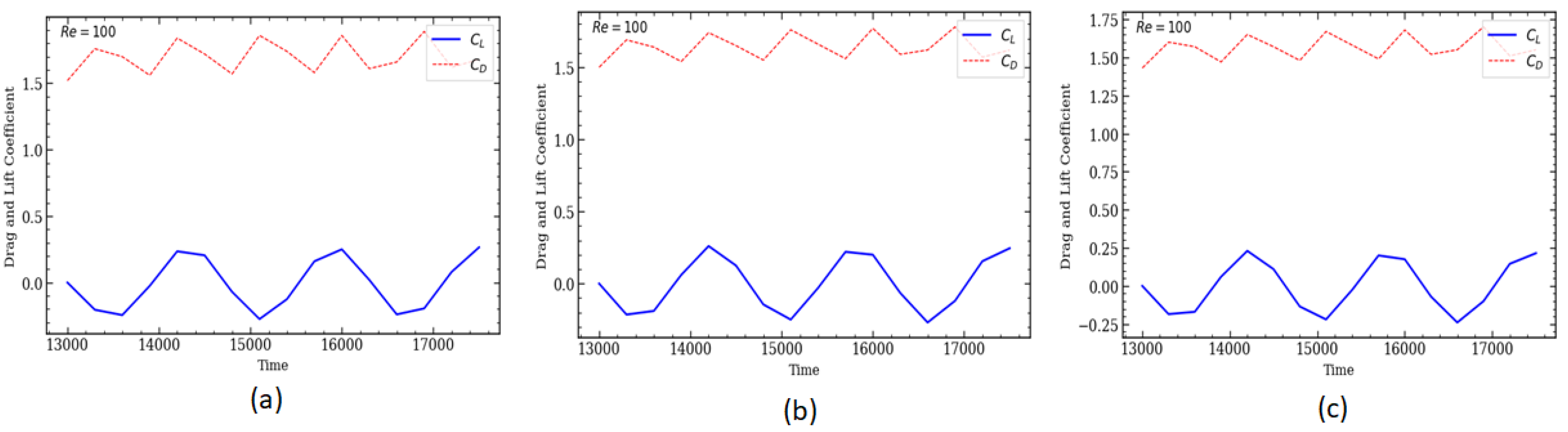
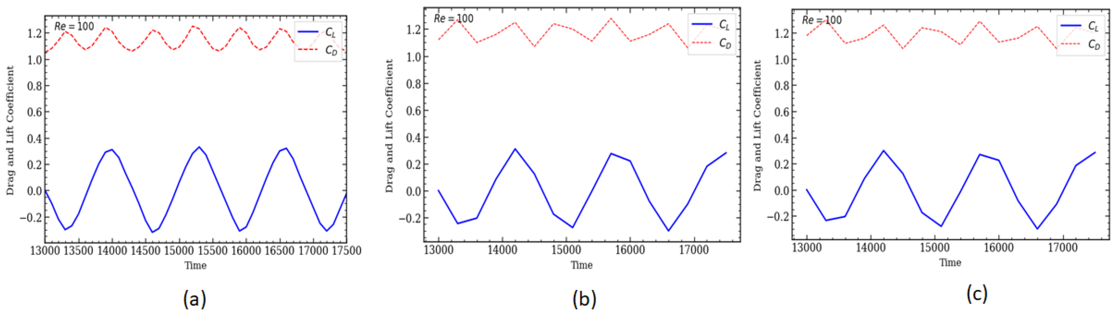
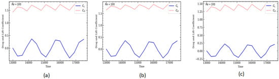
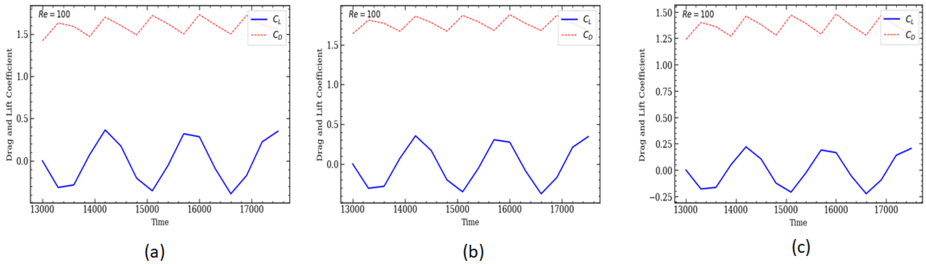
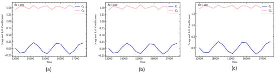
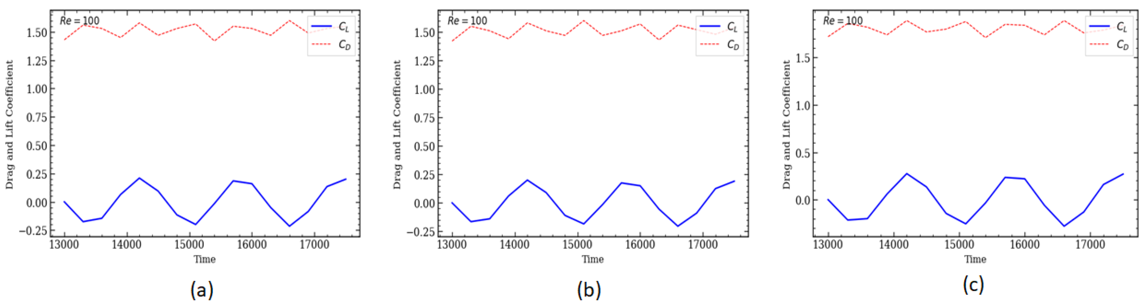
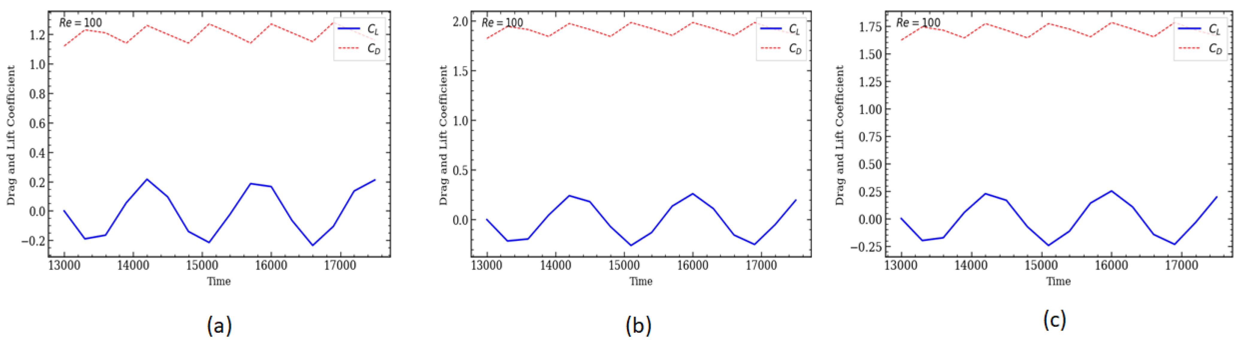
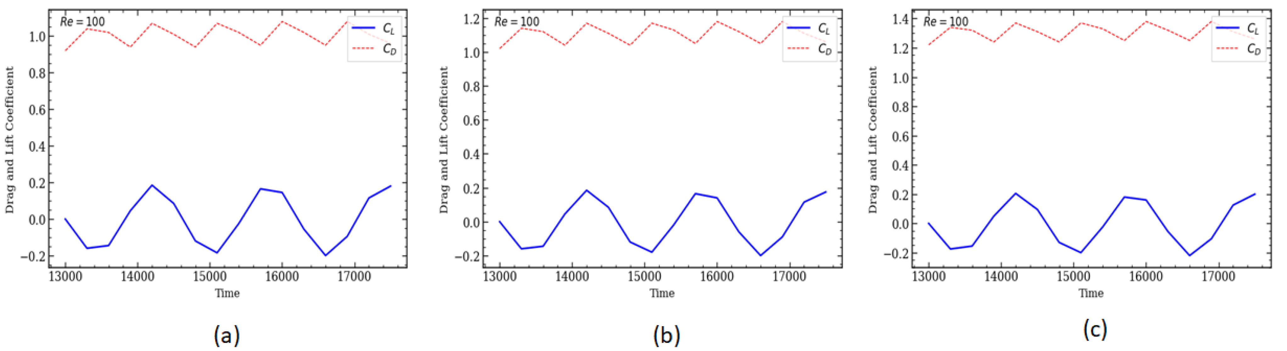
This section will address the intricacies of flow patterns, namely, the lift (C_L) and drag (C_D) coefficients for cylinders, which show some variation in these flow patterns under the specified conditions. To further highlight the effects of the blockage ratio on the forces on two cylinders, the C_D and C_L are shown in Figure 11, Figure 12, Figure 13, Figure 14, Figure 15 and Figure 16.

Figure 11. Variation of the C_D and C_L with a fixed Reynolds number and D = 20 for a circular cylinder at different positions: (a) Upstream obstacle position L/4, (b) Central obstacle position L/2, (c) Downstream obstacle position 3L/4.

Figure 12. Variation of the C_D and C_L with a fixed Reynolds number and D = 40 for a circular cylinder at different positions: (a) Upstream obstacle position L/4, (b) Central obstacle position L/2, (c) Downstream obstacle position 3L/4.

Figure 13. Variation of the C_D and C_L with a fixed Reynolds number and D = 60 for a circular cylinder at different positions: (a) Upstream obstacle position L/4, (b) Central obstacle position L/2, (c) Downstream obstacle position 3L/4.

Figure 14. Variation of the C_D and C_L with a fixed Reynolds number and D = 20 for a square cylinder at different positions: (a) Upstream obstacle position L/4, (b) Central obstacle position L/2, (c) Downstream obstacle position 3L/4.

Figure 15. Variation of the C_D and C_L with a fixed Reynolds number and D = 40 for a square cylinder at different positions: (a) Upstream obstacle position L/4, (b) Central obstacle position L/2, (c) Downstream obstacle position 3L/4.

Figure 16. Variation of the C_D and C_L with a fixed Reynolds number and D = 60 for a square cylinder at different positions: (a) Upstream obstacle position L/4, (b) Central obstacle position L/2, (c) Downstream obstacle position 3L/4.

3.3.1. Circular Shape

To further highlight the effect of the blockage on the forces of a circular cylinder at different sizes and positions, the C_D and C_L are described in Figure 11, Figure 12 and Figure 13. As described in Figure 11, one can see that the C_D of the circular cylinder varies with position in all cases (D = 20 LU, 40 LU, and 60 LU).

As illustrated in Figure 11, Figure 12 and Figure 13, the drag coefficient C_D varies in all configurations, reflecting the unsteady nature of the flow and the continuous influence of wake structures on the hydrodynamic drag. For D = 20 LU, significant variations are observed, particularly at L/4 and L/2, where C_D reaches instantaneous values of approximately 2.0 and 1.7, respectively. For D = 40 LU, the drag coefficient also exhibits pronounced fluctuations, with maximum values of approximately 1.6 at L/4 and 3L/4. For D = 60 LU, the fluctuations are generally less pronounced, although a peak close to 1.4 is observed at L/2. These results indicate that both the obstacle diameter and its longitudinal position significantly modify the hydrodynamic resistance. Increasing the obstacle diameter increases the blockage ratio and consequently alters the velocity distribution, pressure field, and wake development. Nevertheless, the variation of C_D with diameter is not strictly monotonic, demonstrating that the drag is governed by the combined effects of obstacle size, position, confinement, and wake dynamics. The displacement of the cylinder toward 3L/4 also modifies the available downstream distance for wake development and pressure recovery, resulting in distinct drag fluctuations. Overall, the results confirm that the longitudinal position and size of the circular obstacle are important parameters controlling the drag characteristics of confined flow.

The effect of the position and size of the circular cylinder is represented in Table 3. The increase in blockage ratio causes a linear decrease in drag coefficient values. This is because when the blockage ratio increases, the flow behavior becomes similar to unconfined flow, which lowers the pressure applied to the cylinder wall and causes viscous dissipation. Consistent with physical phenomena, the drag coefficient values increase with position and also with obstacle size.

Table 3. Mean drag coefficient for the flow over a circular cylinder at Re = 100.

Position and Size		CD
	D = 20	2
L/4	D = 40	1.7
	D = 60	1.5
	D = 20	1.6
L/2	D = 40	1.4
	D = 60	1.8
	D = 20	1.6
3L/4	D = 40	1.5
	D = 60	1.3

3.3.2. Square Shape

To further highlight the effect of size and position on the force square cylinder, the C_D and C_L are described in Figure 14, Figure 15 and Figure 16. The profiles of C_D and C_L are different from those in the circular cylinder case because of the square edge in the flow.

At the start of the simulation, the three configurations display a very high value of C_D, due to the rapid establishment of the flow field around the sharp edges of the square.

As illustrated in Figure 14, Figure 15 and Figure 16, the drag coefficient C_D exhibits noticeable temporal fluctuations for all square obstacle configurations, reflecting the unsteady nature of the flow and the continuous interaction between the obstacle and the wake structures. For D = 20 LU, the drag coefficient shows significant variations at all three positions. At L/4, the drag coefficient increases rapidly and reaches an instantaneous peak of approximately 1.6, while at L/2, a maximum value of approximately 1.5 is observed. At 3L/4, the drag coefficient reaches a higher peak of approximately 1.8, indicating a stronger instantaneous drag response when the obstacle is located closer to the outlet.

For D = 40 LU, pronounced fluctuations are also observed. At L/4, C_D varies mainly between approximately 0.7 and 1.2, whereas at L/2, it increases sharply to approximately 1.8 before gradually decreasing. At 3L/4, the drag coefficient exhibits several pronounced peaks, reaching approximately 1.5–1.6. For D = 60 LU, the temporal fluctuations are comparatively moderate at L/4 and L/2, with C_D generally remaining around 0.9–1.2. At 3L/4, however, the coefficient remains relatively high, reaching values close to 1.2.

Figure 14, Figure 15 and Figure 16 show that C_L exhibits exactly one trough and one crest per time period, since C_L is strongly affected by the pressure distribution on the top and bottom sides of the cylinder, which is itself governed by vortex shedding. Owing to this close relationship with the growth and shedding of the eddies, the lift force fluctuation’s value varies between a positive maximum and a negative maximum of equal size.

Table 4 displays the average drag coefficient and coefficient of lift for Re = 100. The numerical findings currently available are in good agreement with all of the results computed using the existing LBM.

Table 4. Mean drag coefficient for the flow over a square cylinder at Re = 100.

Position and Size		CD
	D = 20	1.6
L/4	D = 40	1.2
	D = 60	0.9
	D = 20	1.5
L/2	D = 40	1.8
	D = 60	1.2
	D = 20	1.8
3L/4	D = 40	1.6
	D = 60	1.2

These results demonstrate that the drag coefficient of the obstacle is strongly affected by both obstacle size and longitudinal position. Increasing the obstacle diameter increases the blockage ratio, thereby modifying the velocity distribution, pressure field, and wake development around the obstacle.

Compared with the circular obstacle, the square obstacle generally produces stronger flow disturbances due to its sharp corners, which promote earlier flow separation and stronger pressure gradients. Consequently, the temporal evolution of C_D exhibits pronounced fluctuations, particularly for larger blockage ratios and for specific obstacle positions.

4. Discussion

The present results highlight the strong influence of obstacle position, size, and geometry on the flow characteristics in a confined channel. For both circular and square obstacles, moving the obstacle toward the outlet progressively intensifies flow separation, recirculation, and confinement effects, leading to higher drag coefficients. This behavior can be attributed to the reduction in the available downstream space, which modifies the wake development and increases the interaction between the separated flow and the channel boundaries. Increasing the obstacle size further strengthens these effects by reducing the effective flow passage and increasing the blockage ratio. A clear difference is also observed between the two geometries—the sharp corners of the square obstacle promote earlier flow separation and generate a wider and more disturbed wake than the circular obstacle, resulting in generally higher drag levels. These observations indicate that obstacle position and size cannot be considered independently when assessing confined flows, since their combined effects significantly modify the wake dynamics and hydrodynamic forces. The comparison between the two geometries therefore demonstrates that obstacle shape is an additional controlling factor that should be considered when optimizing the configuration of confined flow systems.

5. Conclusions

In this paper, LBM simulations were carried out for flow past a circular and square cylinder confined in a channel. In this work, for a fixed Reynolds number, the effects of two parameters on flow behavior are studied, namely, position and cylinder size. The simultaneous investigation of obstacle position and size for circular and square geometries enables a detailed assessment of how these parameters interact with channel confinement to modify flow structure and hydrodynamic forces. For an upstream obstacle position of L/4, it is obviously observed that the location of the obstacle is too far upstream to affect the wake, and vortex shedding only occurs at the upper and lower edges of the obstacle. The flow behaves as a single structure with a huge characteristic length. The separation, recirculation, and confinement phenomena gradually become more intense as the cylinder is at L/2 and 3L/4.

The drag coefficient strongly depends on the position of the cylinder, while the drag values increase at L/2 and more at 3L/4, but have little effect at L/4.

The findings demonstrate that the effects of the confinement are dramatically enhanced, and the wake structure is significantly altered by increasing the obstacle’s size.

In comparison, the square obstacle generates earlier flow separations due to its sharp edges, producing a wider and more unstable wake as well as generally higher drag levels. Thus, although both geometries show an increase in C_D with position in the channel, the square obstacle induces more marked hydrodynamic effects than the cylinder due to its angular geometry.

References

- Mohamad, A.A. Applied Lattice Boltzmann Method for Transport Phenomena, Momentum, Heat and Mass Transfer. Can. J. Chem. Eng. 2007, 85, 946–947. [Google Scholar] [CrossRef] [Scilit]
- Asinari, P.; Ohwada, T. Current Status of Lattice Boltzmann Methods Applied to Aerodynamic, Aeroacoustic, and Thermal Flows. Prog. Aerosp. Sci. 2020, 115, 100616. [Google Scholar] [CrossRef] [Scilit]
- Li, Q.; Xing, Y.; Huang, R. Equations of State in Multiphase Lattice Boltzmann Method Revisited. Phys. Rev. E 2023, 107, 015301. [Google Scholar] [CrossRef] [Scilit] [PubMed]
- Bayat, A.; D’Orazio, A.; Soufivand, M. A Systematic Review of Lattice Boltzmann Techniques for Compressible Flow Model-ling. Eng. Appl. Comput. Fluid Mech. 2026, 20, 2647567. [Google Scholar] [CrossRef] [Scilit]
- Lallemand, P.; Luo, L.-S.; Krafczyk, M.; Yong, W.-A. The Lattice Boltzmann Method for Nearly Incompressible Flows. J. Comput. Phys. 2021, 431, 109713. [Google Scholar] [CrossRef] [Scilit]
- Succi, S. Lattice Fluid Dynamics: Thirty-five Years Down the Road. Comptes Rendus. Mécanique 2022, 350, 207–218. [Google Scholar] [CrossRef] [Scilit]
- Krüger, T.; Kusumaatmaja, H.; Kuzmin, A.; Shardt, O.; Silva, G.; Viggen, E.M. The Lattice Boltzmann Method; Springer: Cham, Switzerland, 2017. [Google Scholar] [CrossRef] [Scilit]
- Grucelski, A.; Pozorski, J. Lattice Boltzmann Simulations of Heat Transfer in Flow Past a Cylinder and in Simple Porous Media. Int. J. Heat Mass Transf. 2015, 86, 139–148. [Google Scholar] [CrossRef] [Scilit]
- Bhatnagar, P.L.; Gross, E.P.; Krook, M. A Model for Collision Processes in Gases. I. Small Amplitude Processes in Charged and Neutral One-Component Systems. Phys. Rev. 1954, 94, 511–525. [Google Scholar] [CrossRef] [Scilit]
- d’Humières, D. Generalized Lattice-Boltzmann Equations. In Rarefied Gas Dynamics: Theory and Applications; Shizgal, B.D., Weaver, D.P., Eds.; American Institute of Aeronautics and Astronautics: Washington, DC, USA, 1992; pp. 450–458. [Google Scholar] [CrossRef] [Scilit]
- Lallemand, P.; Luo, L.-S. Theory of the Lattice Boltzmann Method: Dispersion, Dissipation, Isotropy, Galilean Invariance, and Stability. Phys. Rev. E 2000, 61, 6546–6562. [Google Scholar] [CrossRef] [Scilit] [PubMed]
- Jiang, C.; Zhou, H.; Xia, M.; Tang, J.; Jiang, S.; Zhang, M. Stability Conditions of Multiple-Relaxation-Time Lattice Boltzmann Model for Seismic Wavefield Modeling. J. Appl. Geophys. 2022, 204, 104742. [Google Scholar] [CrossRef] [Scilit]
- Chai, Z.; Shi, B. Multiple-Relaxation-Time Lattice Boltzmann Method for the Navier-Stokes and Nonlinear Convec-tion-Diffusion Equations: Modeling, Analysis, and Elements. Phys. Rev. E 2020, 102, 023306. [Google Scholar] [CrossRef] [Scilit] [PubMed]
- Hosseini, S.A.; Karlin, I.V. Lattice Boltzmann for Non-Ideal Fluids: Fundamentals and Practice. Phys. Rep. 2023, 1030, 1–137. [Google Scholar] [CrossRef] [Scilit]
- Wu, J.-S.; Shao, Y.-L. Simulation of Flow Past a Square Cylinder by Parallel Lattice Boltzmann Method Using Multi-Relaxation-Time Scheme. J. Mech. 2006, 22, 35–42. [Google Scholar] [CrossRef] [Scilit]
- Strniša, F.; Urbic, T.; Plazl, I. A Lattice Boltzmann Study of 2D Steady and Unsteady Flows around a Confined Cylinder. J. Braz. Soc. Mech. Sci. Eng. 2020, 42, 103. [Google Scholar] [CrossRef] [Scilit]
- Lallemand, P.; Luo, L.-S. Theory of the Lattice Boltzmann Method: Acoustic and Thermal Properties in Two and Three Dimensions. Phys. Rev. E 2003, 68, 036706. [Google Scholar] [CrossRef] [Scilit] [PubMed]
- Hamane, D.; Guerri, O.; Larbi, S. Investigation of Flow around a Circular Cylinder in Laminar and Turbulent Flow Using the Lattice Boltzmann Method. In AIP Conference Proceedings; AIP Publishing LLC: Melville, NY, USA, 2014; Volume 1648, p. 020015. [Google Scholar] [CrossRef] [Scilit]
- Fezai, S.; Oueslati, F.; Ben-Beya, B. Influence of Various Staggered Arrangements of Square Cylinders on Drag and Lift Forces and Wake Flow Behavior. Int. J. Fluid Mech. Res. 2021, 48, 73–91. [Google Scholar] [CrossRef] [Scilit]
- Refaie Ali, A.; Abbasi, W.S.; Younus, R.; Rahman, H.; Nadeem, S.; Majeed, A.H.; Ahmad, I. Enhancing Hydrodynamic Forces through Miniaturized Control of Square Cylinders Using the Lattice Boltzmann Method. Sci. Rep. 2024, 14, 15524. [Google Scholar] [CrossRef] [Scilit] [PubMed]
- Refaie Ali, A.; Abbasi, W.S.; Bibi, B.; Rahman, H.; Ul Islam, S.; Majeed, A.H.; Ahmad, I. Spacing Effects on Flows around Two Square Cylinders in Staggered Arrangement via LBM. Sci. Rep. 2024, 14, 18049. [Google Scholar] [CrossRef] [Scilit] [PubMed]
- Granados-Ortiz, F.-J. A Novel Comprehensible Non-Intrusive Sensitivity-Driven Additive Aerodynamic Shape Optimization (AASO) and Its Implementation Using the Lattice Boltzmann Method (AASO-LBM). Sci. Rep. 2025, 15, 41845. [Google Scholar] [CrossRef] [Scilit] [PubMed]
- Hussain, A.; Celik, B. Conjugate Heat Transfer Analyses via a Lattice Boltzmann Method Solver for Time-Periodic Flows over a Conductive Square Cylinder Confined in a Channel. Phys. Fluids 2026, 38, 063604. [Google Scholar] [CrossRef] [Scilit]
- Wissocq, G.; Sagaut, P. Hydrodynamic Limits and Numerical Errors of Isothermal Lattice Boltzmann Schemes. J. Comput. Phys. 2022, 450, 110858. [Google Scholar] [CrossRef] [Scilit]
- Li, X.; Shan, X.; Duan, W. Theoretical Progress on Regularized Lattice Boltzmann Collision Models. Acta Aerodyn. Sin. 2022, 40, 46–64. [Google Scholar] [CrossRef]
- Mohamad, A.A. Lattice Boltzmann Method: Fundamentals and Engineering Applications with Computer Codes; Springer: London, UK, 2019. [Google Scholar] [CrossRef] [Scilit]
- Kaushal, S.; Succi, S.; Ansumali, S. Flow Force Calculation in the Lattice Boltzmann Method. Phys. Rev. E 2023, 108, 045304. [Google Scholar] [CrossRef] [Scilit] [PubMed]
- Wang, S.; Wu, X.; Peng, C.; Chen, S.; Liu, H. Analysis on the Force Evaluation by the Momentum Exchange Method and a Localized Refilling Scheme for the Lattice Boltzmann Method. Comput. Math. Appl. 2025, 183, 180–199. [Google Scholar] [CrossRef] [Scilit]
- Braza, M.; Chassaing, P.; Minh, H.H. Numerical Study and Physical Analysis of the Pressure and Velocity Fields in the Near Wake of a Circular Cylinder. J. Fluid Mech. 1986, 165, 79–130. [Google Scholar] [CrossRef] [Scilit]
- Calhoun, D. A Cartesian Grid Method for Solving the Two-Dimensional Streamfunction-Vorticity Equations in Irregular Regions. J. Comput. Phys. 2002, 176, 231–275. [Google Scholar] [CrossRef] [Scilit]
- Perumal, D.A.; Kumar, G.V.S.; Dass, A.K. Lattice Boltzmann Simulation of Flow over a Circular Cylinder at Moderate Reynolds Numbers. Therm. Sci. 2014, 18, 1235–1246. [Google Scholar] [CrossRef] [Scilit]
- Breuer, M.; Bernsdorf, J.; Zeiser, T.; Durst, F. Accurate Computations of the Laminar Flow Past a Square Cylinder Based on Two Different Methods: Lattice-Boltzmann and Finite-Volume. Int. J. Heat Fluid Flow 2000, 21, 186–196. [Google Scholar] [CrossRef] [Scilit]
- Sahu, A.K.; Chhabra, R.P.; Eswaran, V. Two-Dimensional Unsteady Laminar Flow of a Power Law Fluid across a Square Cylinder. J. Non-Newton. Fluid Mech. 2009, 160, 157–167. [Google Scholar] [CrossRef] [Scilit]
- Zhou, Y.; Wang, Z.; Qian, Y.; Yang, H.; Wei, Y. Numerical Simulation of the Flow around Two Square Cylinders Using the Lattice Boltzmann Method. Phys. Fluids 2021, 33, 037110. [Google Scholar] [CrossRef] [Scilit]
Disclaimer/Publisher’s Note: The statements, opinions and data contained in all publications are solely those of the individual author(s) and contributor(s) and not of MDPI and/or the editor(s). MDPI and/or the editor(s) disclaim responsibility for any injury to people or property resulting from any ideas, methods, instructions or products referred to in the content. |
© 2026 by the authors. Licensee MDPI, Basel, Switzerland. This article is an open access article distributed under the terms and conditions of the Creative Commons Attribution (CC BY) license.