Finite Element-Assisted Random Forest Modeling for Development of Weld Schedules in Multi-Cycle Resistance End-Closure Welding of Zircaloy-4 Nuclear Fuel Elements

Abstract

Resistance end-closure welding of Zircaloy-4 nuclear fuel elements is a critical operation in Pressurized Heavy Water Reactor fuel fabrication. Weld quality and dimensional integrity depend on upset formation, reflecting combined effects of heat generation and forging during welding. Control of pre-heat upset is essential for establishing intimate contact at the faying surfaces, whereas total upset must be maintained within specified limits to satisfy dimensional requirements for fuel bundle assembly. In the present study, Random Forest (RF) regression models were developed to predict pre-heat and total upset. A comprehensive dataset was generated using a validated Finite Element (FE) model by varying pre-heat current, post-heat current, pre-heat duration, post-heat duration, and squeeze force over the practical operating range. The RF hyperparameters were optimized using a coarse-to-fine grid search strategy with five-fold cross-validation and Root Mean Square Error (RMSE) as the optimization metric. The optimized models were evaluated using an independent blind-test dataset and achieved RMSE values of 0.06 mm for pre-heat upset and 0.08 mm for total upset. The validated models rapidly screened 4725 full-factorial weld schedules and identified candidate schedules whose predicted responses satisfied the required upset criteria. Experimental verification demonstrated good agreement with the model predictions. The proposed FE–RF approach provides an efficient tool for weld-schedule development in nuclear fuel manufacturing while reducing the need for extensive simulations and experiments.

1. Introduction

Pressurized Heavy Water Reactors (PHWRs) are fueled with bundles assembled from fuel elements containing natural uranium dioxide pellets encapsulated in Zircaloy-4 (Zr-4) clad tubes. Fuel-element integrity depends on the quality of the end-closure welds joining the Zr-4 end caps to the clad tubes. These welds act as the primary barrier against the release of fission products during reactor operation. Consequently, stringent dimensional and metallurgical requirements are imposed on the end-closure welds to ensure fuel integrity throughout their service life in the reactor [1,2,3].

Resistance welding is extensively employed for end-closure welding because of its high productivity, localized heat generation, and suitability for automated manufacturing machinery [4,5]. Weld quality depends on the complex interaction among welding current, duration, and squeeze force [6,7]. Among the various responses characterizing end-closure welding, upset formation is an important indicator of process stability and weld quality. Upset represents axial shortening caused by material softening, radial expansion, and forging action during welding. In practice, both insufficient and excessive upset are undesirable. Insufficient upset indicates inadequate interfacial heating and incomplete consolidation, whereas excessive upset results in excessive material flow and dimensional deviations. Hence, accurately predicting and controlling upset formation are essential for maintaining dimensional tolerances and ensuring consistent weld quality during the production of PHWR fuel elements. The length of each end-closed welded fuel element shall be maintained within the required tolerance to facilitate the bundle assembly. Accordingly, the required total upset is between 1.1 mm and 1.2 mm.

Numerical simulation techniques based on the Finite Element Method (FEM) have been used for welding-process development [8,9,10,11,12], providing insights into temperature evolution, material flow, and upset development. New FEM-based simulation methodologies have been developed to reduce computational time and improve predictive accuracy [13,14,15,16,17]. Nevertheless, FE simulations remain computationally intensive, particularly when a large number of parameter combinations must be explored.

Machine learning (ML) techniques have emerged as efficient surrogate models for predicting manufacturing-process responses directly from experimental or simulation datasets [18,19,20,21,22,23]. Among the various ML algorithms, Random Forest (RF) regression has attracted considerable attention in manufacturing applications because of its ability to accurately capture nonlinear relationships among process variables using the relatively small datasets common in engineering applications [24,25]. Unlike a single decision tree, RF uses bootstrap aggregation and random feature selection to construct an ensemble of predictors, thereby reducing variance and minimizing the risk of overfitting. Previous studies have successfully employed RF models for prediction of welding quality and mechanical properties with high accuracy [26,27].

Previous numerical investigations on zirconium-alloy tube-end plug welding [28,29] have established usefulness of coupled electro-thermal–mechanical FE modeling for analyzing temperature evolution and joint formation. However, these studies have focused on the mechanistic understanding of individual welding conditions or limited parameter variations. For production weld-schedule development, a much larger multidimensional process space must be explored because current, heating duration, and squeeze force interact nonlinearly to determine the final upset. Moreover, FE-assisted ML modeling remains insufficiently explored for this application.

The present study addresses these limitations by developing RF regression models to predict pre-heat upset and total upset during multi-cycle resistance end-closure welding of Zr-4 nuclear fuel elements. A validated FE model was employed to generate the training dataset, thereby minimizing the need for extensive welding experiments. Separate RF models were developed for the two upset responses because they represent distinct stages of weld deformation. The RF hyperparameters were optimized using a systematic coarse-to-fine grid search with five-fold cross-validation (5-fold CV). The predictive capability of the optimized models was evaluated using an independent blind-test dataset. Finally, the validated models were used for rapid full-factorial exploration of the welding parameter space to identify candidate schedules satisfying the specified upset requirements, followed by experimental verification of representative schedules.

2. Materials and Methods

2.1. Welding Procedure

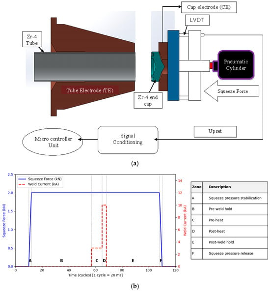
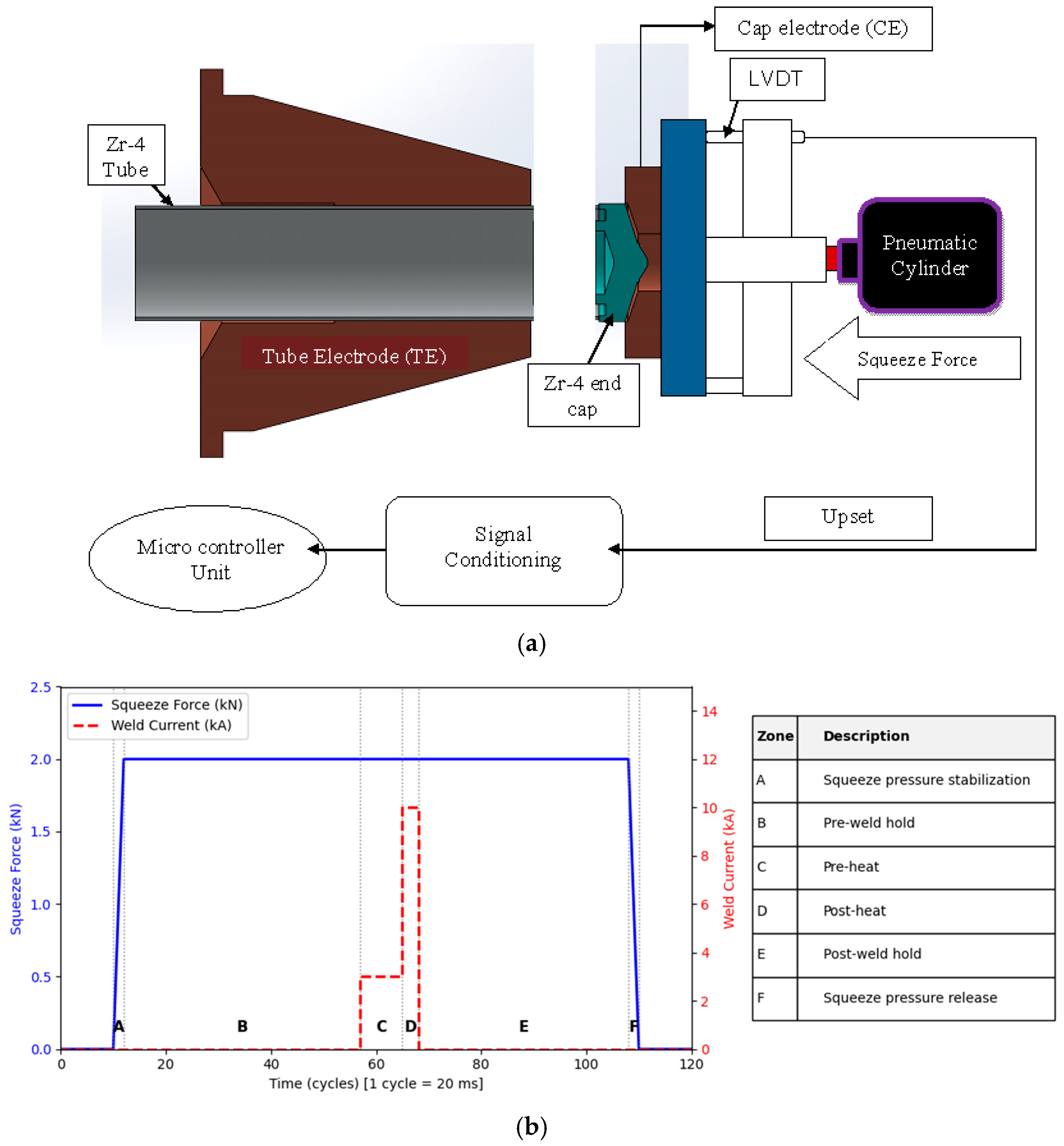
The clad tubes and end caps are fabricated from Zr-4 at Nuclear Fuel Complex, Hyderabad, India. Each tube is 485 mm long, with an outer diameter of 13 mm and a wall thickness of 0.4 mm. The Tube Electrode (TE) and Cap Electrode (CE) are made of RWMA Class-12 and Class-3 copper alloys, respectively. In the welding setup shown in Figure 1a, the tube is rigidly held in the fixed TE (collet), whereas the end cap is held in the movable CE, which is actuated by a pneumatic cylinder to apply the required squeeze force at the faying interface.

Figure 1. (a) Tube-cap weld fitment and upset measurement. (b) Weld schedule.

The welding schedule consists of squeeze, weld, and post-weld hold stages (Figure 1b). During the squeeze stage (pre-weld hold), only the squeeze force is applied to smoothen surface asperities before current application. During the weld stage, two different current pulses are given sequentially under a constant squeeze force: a low current, termed the ‘pre-heat current’, promotes interfacial conditioning and establishes uniform contact, followed by a high current, termed the ‘post-heat current’, which generates rapid resistive heating and joint formation. During the post-weld hold stage, the squeeze force is maintained to assist joint consolidation. Of the seven input parameters, pre-weld squeeze time and hold time were kept constant in the present study.

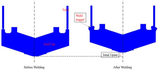
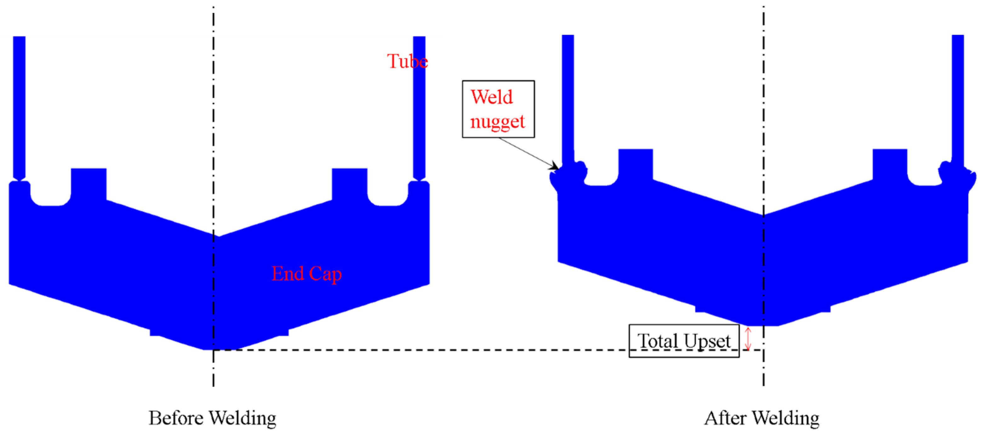
During resistance welding, axial deformation occurs primarily in the cap and the protruding tube edge, while the adjoining cap material flows radially inward and outward to form the weld nugget shown in Figure 2. The resulting axial deformation is termed ‘total upset’ (Figure 2) and is measured in situ during welding using a Linear Variable Differential Transducer (LVDT) connected to the movable CE. The axial deformation occurring during the pre-heat weld stage is termed ‘pre-heat upset’ and is obtained from the deformation signature recorded by the LVDT.

Figure 2. Weld nugget.

2.2. Welding Simulation

The multi-cycle resistance end-closure welding process was simulated using the FE-based software SORPAS 2D, version 12 (Simulation and Optimization of Resistance Projection and Spot Welding Processes) [30]. A fully coupled thermal–mechanical–electrical two-dimensional (2D) axisymmetric FE model was developed. The number of elements was fixed at 3000 based on a mesh-independent study. A finer mesh was used near the tube-cap interface, where dynamic changes were anticipated. Temperature-dependent thermophysical properties of Zr-4 were taken from the literature [31,32,33,34].

Electrical contact resistance at the tube-cap interface was calculated using the pressure-dependent contact-resistivity formulation implemented in SORPAS. Because no explicit oxide, coating, or surface-contamination layer was considered in the present FE model, the contact resistivity was represented as

$${\rho }_{contact}=3\left({\displaystyle \frac{{\sigma }_{s, soft}}{{\sigma }_n}}\right)\left({\displaystyle \frac{{\rho }_1+{\rho }_2}{2}}\right)$$

(1)

Here, σ_s,soft is the flow stress of the softer contacting material; σ_n is the instantaneous normal pressure at the interface, and ρ₁ and ρ₂ are the electrical resistivities of the two contacting materials. Thus, the interface resistance evolves with the mechanical contact conditions during welding: increasing contact pressure lowers the contact resistivity, while temperature-dependent material properties govern the corresponding electrical and thermal responses. No empirical calibration or fitting of the contact resistance was performed in the present study. Instead, the adequacy of the overall electro-thermo-mechanical FE representation was instead assessed by experimentally comparing pre-heat and total upset under representative welding conditions.

The input parameters and levels investigated in the present study are listed in Table 1. Because large-scale experiments and FE simulations are resource-intensive, RF models were developed to predict pre-heat and total upset. The RF training dataset was generated using 50 Latin Hyper Sampling (LHS) simulations and 27 Taguchi L27 simulations. Additional 16 simulations were carried out for independent blind-testing and were completely excluded from model training. LHS [35,36] was adopted to obtain a space-filling distribution across the five-dimensional (5D) process space while minimizing clustering of sampling points. The Taguchi L27 design [37,38,39] supplemented the LHS dataset by introducing structured orthogonal combinations, thereby improving the representation of parameter interactions and boundary conditions. Furthermore, the independent blind-test schedules were deliberately selected to span low, intermediate, and high levels of pre-heat and post-heat currents without overlapping the training dataset. The training (Table S1) and independent blind-test (Table S2) datasets are provided as Supplementary Materials.

Table 1. Process parameters.

Parameter	Level
Pre-heat current (Ipre)	2–5 kA
Post-heat current (Ipost)	9–11 kA
Squeeze force	1.2–2 kN
Pre-weld squeeze time	45 cycles
Pre-heat time (tpre)	5, 6, 7, 8, 9 cycles
Post-heat time (tpost)	1, 2, 3 cycles
Hold time	40 cycles

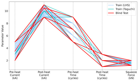
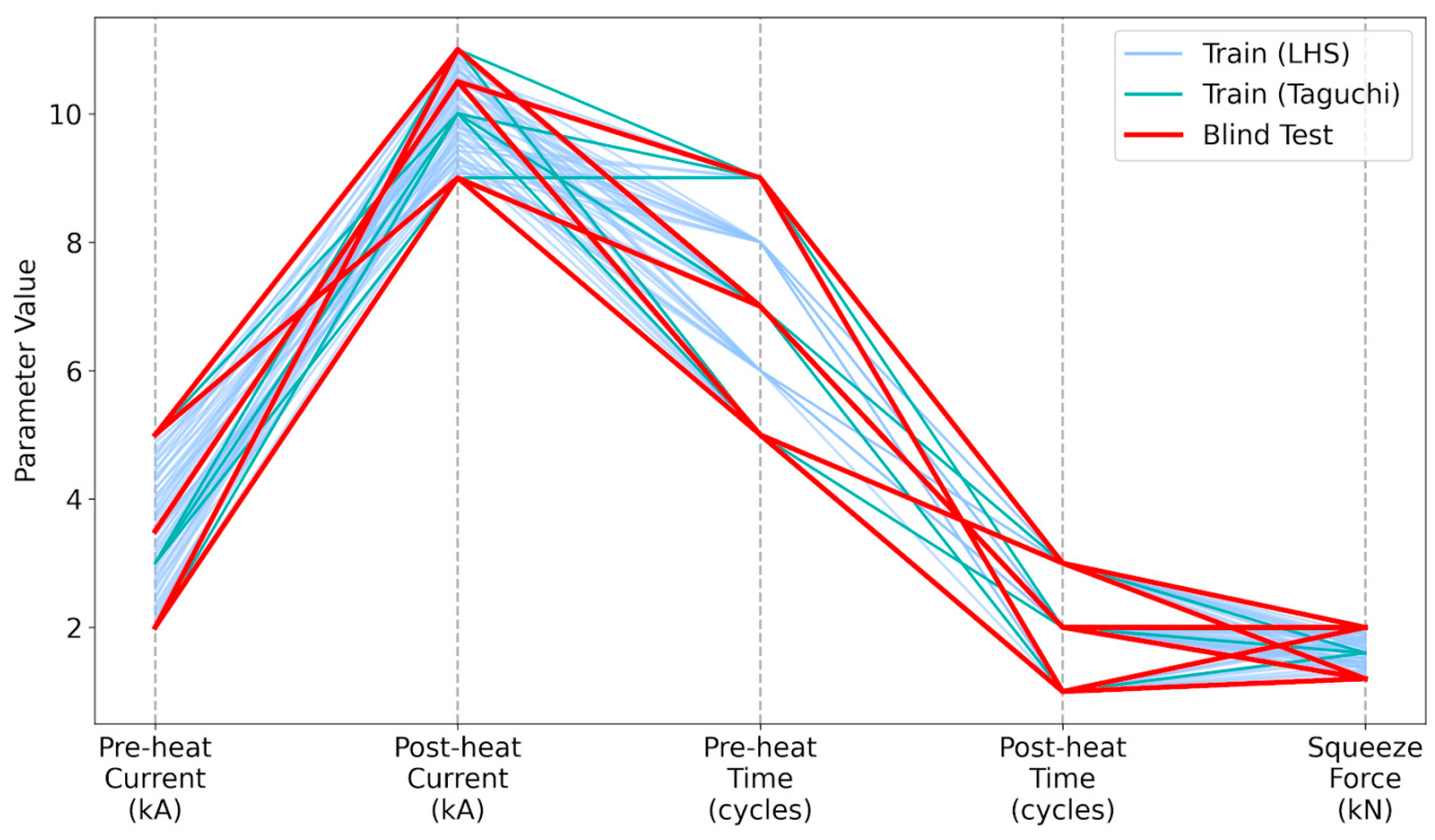
Figure 3 shows the distribution of the training and independent blind-test datasets within the 5D parameter space. Space-filling quality was assessed using the nearest-neighbor Euclidean distance in the normalized 5D parameter space. The minimum (0.195), mean (0.41), and median (0.38) nearest-neighbor distances indicate that the training points are reasonably dispersed. The corresponding minimum (0.901) and mean (0.920) distances indicate broad separation of the independent blind-test schedules across the 5D parameter space.

Figure 3. Uniform coverage of train and independent blind-test dataset across parameter ranges.

2.3. Experimental Validation of Simulation

As FE simulations were used for dataset generation, the FE predictions of pre-heat upset and total upset were validated experimentally. The pre-heat current was fixed at 5 kA (the maximum value), while the remaining four parameters were varied across their respective ranges. The combinations were selected to validate the FE model under low, moderate and high heat input conditions. Helium was used as the inert shielding gas in the experiments.

The FE-predicted and experimentally measured upset values are compared in Table 2. The 2D FE model showed very good agreement with the experiments, with Mean Absolute Percentage Error (MAPE) values of 4% for pre-heat upset and 2% for total upset, indicating that the axisymmetric model adequately captured the dominant deformation behavior. The minor deviations observed can be attributed to the inherent differences between the idealized multi-physics simulation and shop-floor manufacturing conditions. The present 2D axisymmetric model assumes a uniform faying surface and ideal geometric alignments between components. These assumptions can be covered to some extent in 3D modeling which was beyond the scope of the present study. In practice, the native oxide layer on the Zr-4 components and machining-induced surface micro-asperities cause localized fluctuations in contact resistance and non-uniform initial yielding during the pre-heat cycle. Furthermore, although the simulation applies the squeeze force as a perfectly controlled load, the physical pneumatic actuation system possesses inherent inertia, seal friction, and transient follow-up characteristics which affect the rapid material softening in the post-heat phase. Despite these unavoidable shop-floor variations, the FE model successfully captured the governing macroscale thermo-mechanical behavior across the investigated heat input conditions. These results support the use of the validated FE model as the dataset generator for the RF models within the investigated parameter domain.

Table 2. Results of the simulation-validation experiments.

SN	Input Parameters					Output Parameters
	Pre-Heat Current (kA)	Post-Heat Current (kA)	Squeeze Force (kN)	Pre-Heat Time (Cycles)	Post-Heat Time (Cycles)	Pre-Heat Upset (mm)		Total Upset (mm)
						E 1	S 1	E 1	S 1
1	5	11	1.6	9	1	0.74	0.72	1.07	1.06
2	5	9	2	7	1	0.73	0.68	0.9	0.9
3	5	9	1.6	5	3	0.6	0.65	1.08	1.03
4	5	10	2	9	3	0.72	0.71	1.48	1.46
5	5	11	1.2	7	2	0.67	0.7	1.08	1.03
MAPE						0.04		0.02

¹ E: Experimental, S: simulation.

2.4. Random Forest Model

Random Forest (RF) regression was selected to balance predictive capability, robustness, and computational efficiency for this complex resistance-welding process. Further, RF model can also represent nonlinear interactions with limited pre-processing and provides robust ensemble predictions for modest-sized engineering datasets. Other techniques, such as Gaussian Process Regression, Support Vector Regression, and XG Boost, require careful kernel selection and data pre-processing and are susceptible to overfitting the relatively limited size of the dataset in the present study.

Separate RF regression models were developed to predict pre-heat upset and total upset. Their performance is influenced by several hyperparameters controlling forest complexity, tree growth, and bootstrap sampling behavior. Previous studies [40] have demonstrated that the number of trees, tree depth, and feature-sampling strategy affect prediction accuracy and generalization capability. To identify the optimal model configuration, a systematic two-stage coarse-to-fine hyperparameter optimization strategy was adopted. The optimization objective was to minimize the five-fold cross-validation (5-fold CV) Root Mean Square Error (RMSE), which provides a suitable balance between bias and variance estimation for relatively small engineering datasets [41,42]. The available dataset was randomly partitioned into five approximately equal subsets. During each iteration, four subsets were used for model training while the remaining subset is used for validation. The process is repeated five times so that each subset served as the validation set once. Alongside RMSE, Mean Absolute Percentage Error (MAPE) was also calculated to provide a normalized measure of prediction accuracy.

An initial coarse search was conducted over a broad hyperparameter space to identify promising regions of the model performance. The search ranges were selected based on recommendations reported in the RF literature for the datasets of comparable size [43,44] and are summarized in Table 3.

Table 3. Coarse-grid hyperparameter search space used for RF optimization.

SN	Hyperparameter	Coarse Grid Search Range	Fine Grid Search Range
1	Number of trees	50, 100, 200, 300, 500, 1000, 1500, 2000	optimum value ±50 in increments of 25
2	Maximum tree depth	2, 3, 4, 5, 6, 8, 10, None	optimum value ±2
3	Maximum number of features	1, 2, 3, 4, 5	optimum value ±1
4	Minimum samples per leaf	1, 2, 3, 4, 5, 8, 10	optimum value ±3
5	Minimum samples for split	2, 4, 6, 8, 10, 15, 20	optimum value ±5
6	Bootstrap sample fraction	0.5, 0.7, 1.0	optimum value ±0.10 in increments of 0.05

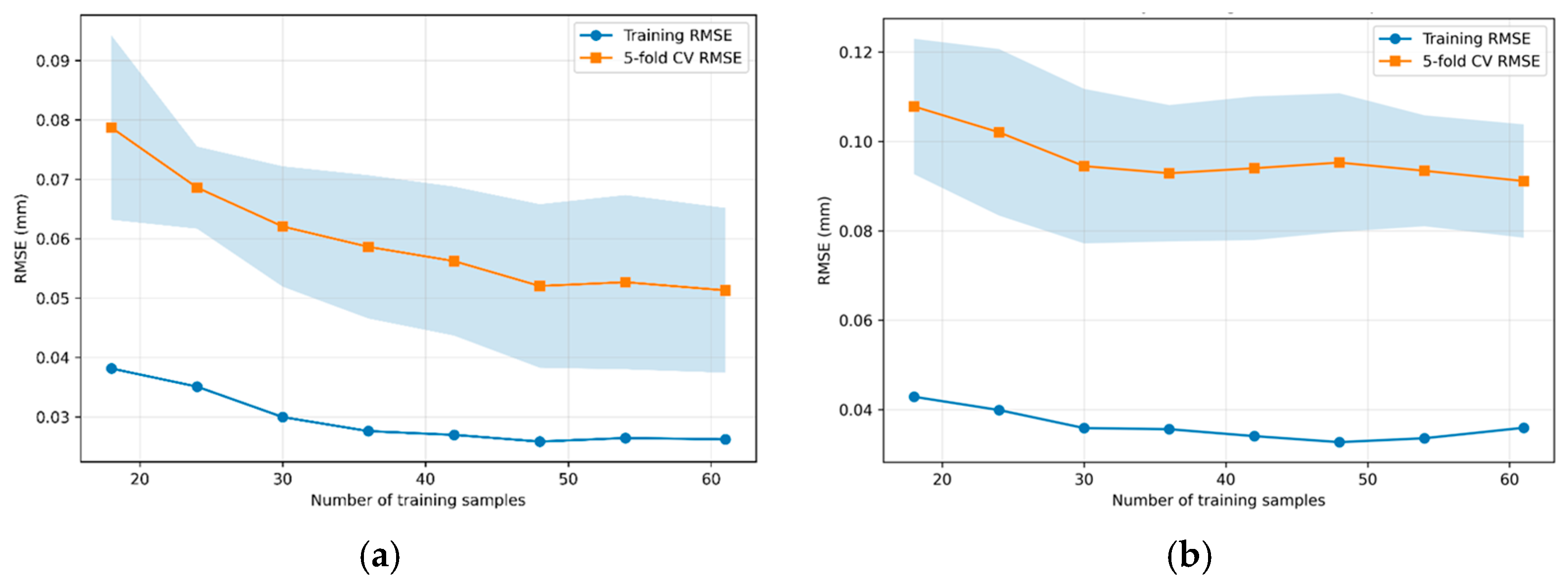
Following identification of the best performing region in the coarse-search stage, a fine grid search was conducted. The aim of the fine grid search is to improve local convergence and obtain an accurate RF model without excessive computational expense. The adequacy of the available training dataset (size: 77) was assessed using learning curves generated by progressively increasing the number of training samples.

The developed RF models are computational surrogates of the experimentally validated FE model. Consequently, their predictive capability inherently depends on the fidelity of the underlying FE model, and uncertainties in the FE model propagate to the RF predictions. Although more extensive experimental validation would further strengthen the FE model, high processing costs and limited machine availability restricted the number of experiments. Accordingly, the FE model was sufficiently validated using representative welding schedules spanning low, intermediate, and high parameter levels. The applicability of the developed RF models is therefore restricted to the investigated parameter space. The models are intended for interpolation within this domain and their reliability at the boundaries and beyond the parameter ranges is limited.

3. Results and Discussions

3.1. Optimization of RF Models

The robustness of the hyperparameter optimization was assessed by repeating the grid search across ten random seeds (0, 10, 20, …, 90), regenerating both the five-fold CV partitions and the internal RF initializations for each iteration. The optimized CV RMSE ranged from 0.049 to 0.054 mm for pre-heat upset, and from 0.087 to 0.102 mm for total upset, respectively. The consistent selection of key hyperparameters across iterations and small fluctuations in prediction error indicate that the optimized configurations lie within a stable performance region rather than at sharp and isolated local minima.

The optimized hyperparameters of the RF models are presented in Table 4.

Table 4. Optimized RF hyperparameters for prediction of pre-heat upset and total upset.

S N	Hyperparameter	Optimized Value for Pre-Heat Upset	Optimized Value for Total Upset
1	Number of trees	300	200
2	Maximum tree depth	8	8
3	Maximum number of features	4	5
4	Minimum samples per leaf	1	1
5	Minimum samples for split	2	2
6	Bootstrap sample fraction	0.7	1.0

The optimization results indicate that moderately deep trees combined with relatively large forest sizes provide the best predictive performance.

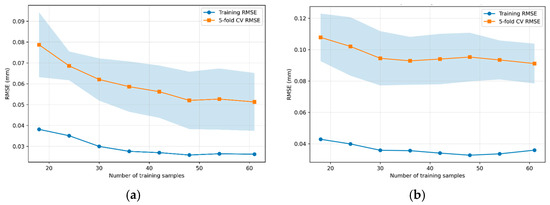
In the learning curves (Figure 4), the convergence of 5-fold CV RMSE indicates diminishing returns beyond approximately 50 training samples suggesting that the available training dataset provides adequate representation of the investigated process space.

Figure 4. Learning curve for prediction of (a) pre-heat upset and (b) total upset.

3.2. Testing of the Optimized RF Models

Table 5 summarizes the predictive accuracy of the optimized RF models during both cross-validation and independent blind-testing. The close agreement between the cross-validation and independent blind-test errors indicates that the optimized models retain their predictive capability for previously unseen welding schedules. Furthermore, the selected hyperparameters provide an appropriate balance between model complexity and generalization performance for the available dataset.

Table 5. Predictive accuracy of the optimized RF models.

Response	CV RMSE (mm)	Independent Blind RMSE (mm)	Independent Blind MAPE (%)
Pre-heat upset	0.05	0.06	10
Total upset	0.09	0.08	6

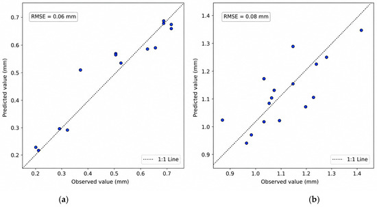
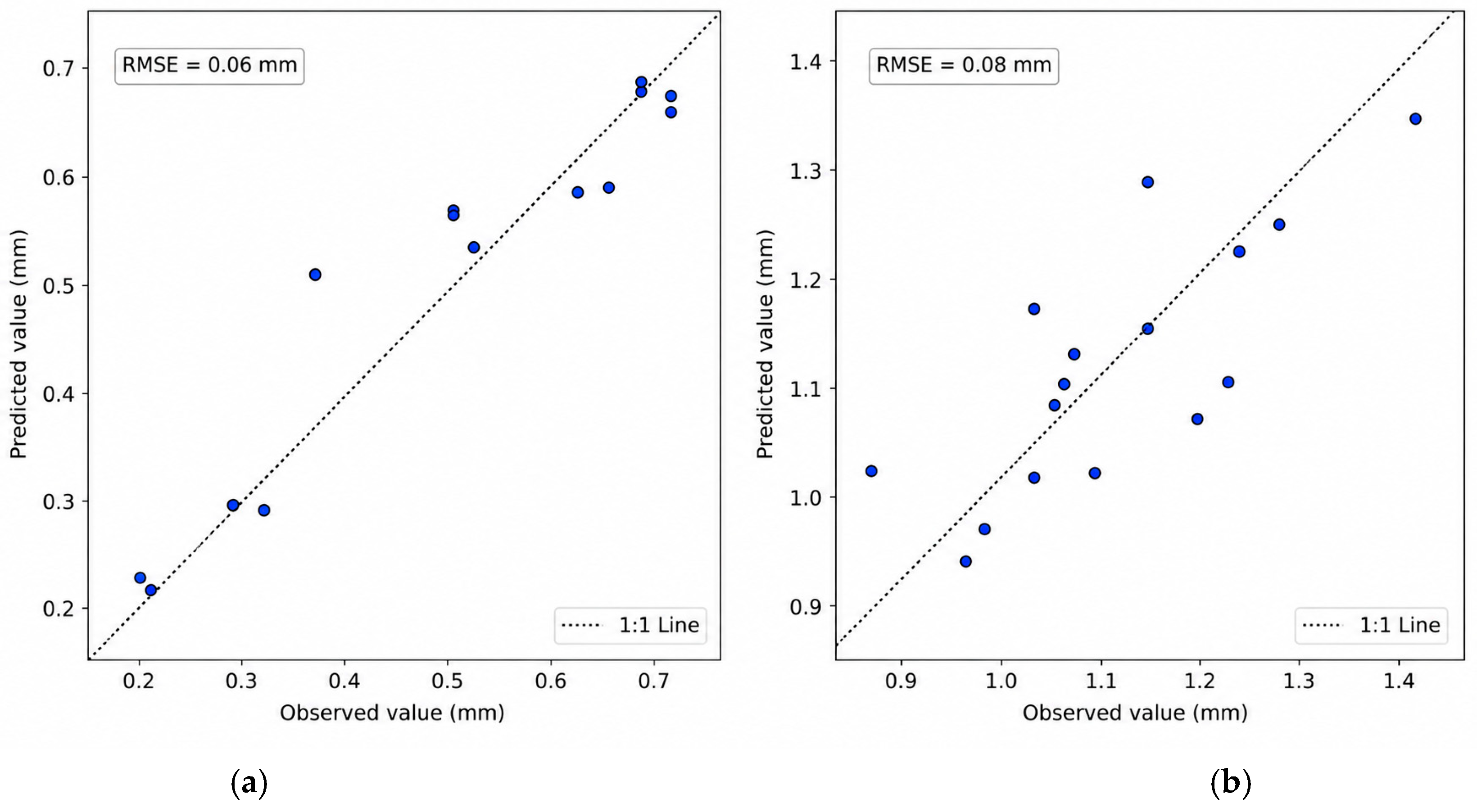
The parity plots in Figure 5 demonstrate close agreement between predicted and observed values. The independent blind-test RMSE and MAPE are sufficiently small for practical engineering process design.

Figure 5. Independent blind-test parity plots for prediction of (a) pre-heat upset and (b) total upset.

Total upset is influenced by simultaneous interactions among pre-heat current, post-heat current, squeeze force, and heating durations. Such coupled thermo-mechanical behavior introduces substantial nonlinearity into the process–response relationship. The low prediction errors obtained in the present study confirm the capability of RF model to effectively capture these complex interactions.

3.3. Identification of Welding Schedules Based on Upset Ranges

The RF models were used to rapidly investigate the input-parameter space through a full-factorial design (Table 6) and identify welding schedules whose predicted responses satisfied the target ranges of 0.55–0.65 mm for pre-heat upset and 1.10–1.20 mm for total upset. Only parameter levels that can be practically implemented on the production welding machine are explored. The resulting full-factorial design contained 4725 welding schedules.

Table 6. Input-parameter ranges for full-factorial exploration.

SN	Input Parameter	Levels
1	Pre-heat current (kA)	2–5 in steps of 0.5
2	Post-heat current (kA)	9–11 in steps of 0.5
3	Pre-heat time (cycles)	5, 6, 7, 8, 9
4	Post-heat time (cycles)	1, 2, 3
5	Squeeze force (kN)	1.2–2 in steps of 0.1

Unlike total upset, which is specified by the dimensional requirements of the fuel element for assembly, no independent acceptance criterion exists for pre-heat upset. The target range of 0.55–0.65 mm was selected based on the thermo-mechanical role of the pre-heating stage. During pre-heating, sufficient axial deformation is required to disrupt oxide film and surface asperities and establish intimate contact between the tube and end cap, promoting stable current transfer before application of the high-current post-heat pulses. Pre-heat upset values below approximately 0.55 mm generally indicate inadequate interfacial conditioning and unstable electrical contact. Conversely, values exceeding 0.65 mm imply excessive deformation during the pre-heat stage, reducing the remaining deformation available during post-heating and increasing the likelihood of over-forging. Accordingly, the range of 0.55–0.65 mm was adopted as a practical engineering window to provide adequate interfacial conditioning while preserving sufficient deformation capacity for controlled joint formation during the subsequent post-heat stage. This range is also consistent with the FE simulations and industrial welding experience, where schedules producing pre-heat upset within this interval generally yielded the required final upset and stable weld formation over a broad range of process parameters.

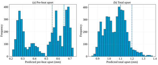
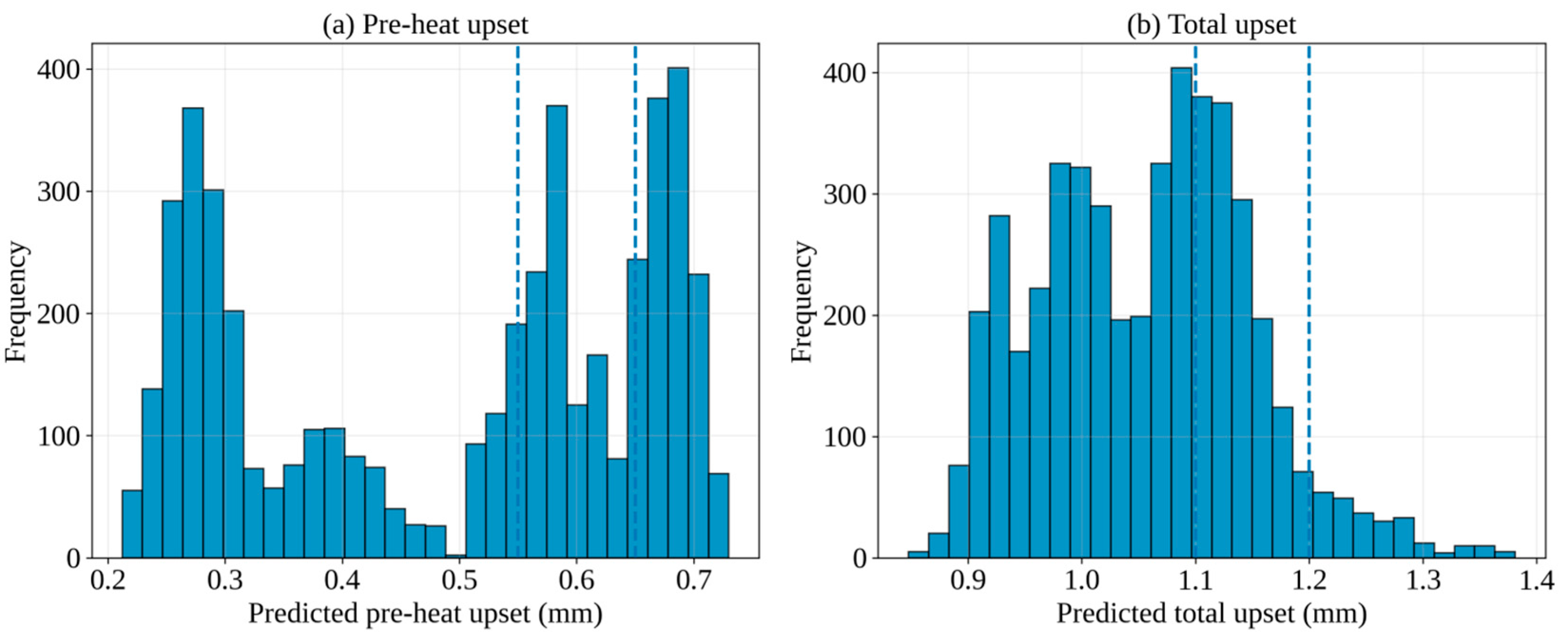
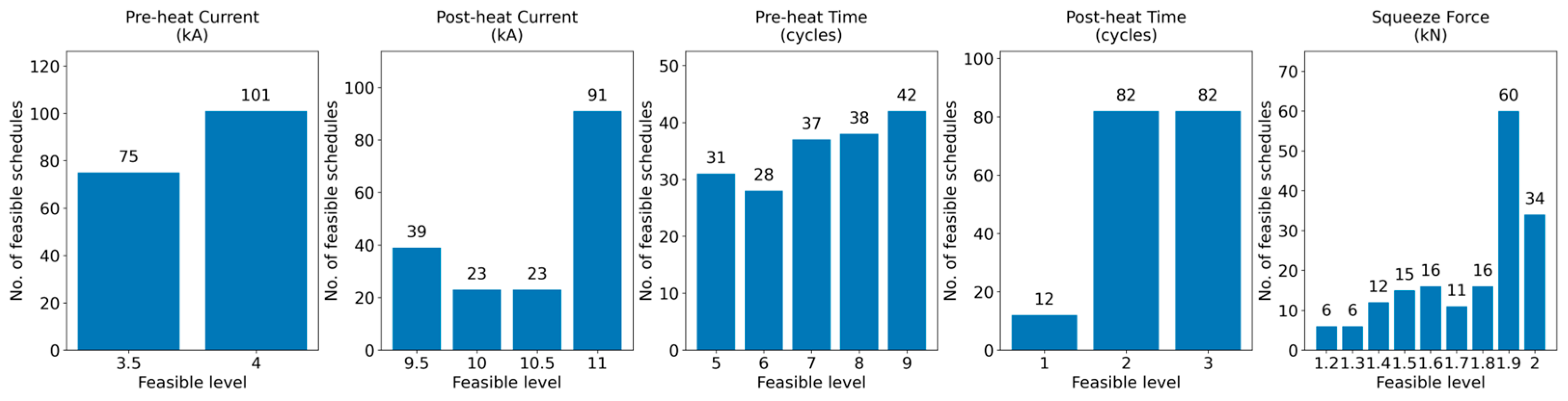
The distribution of predicted values is shown in Figure 6. The RF-assisted full-factorial exploration provided valuable insight into the candidate operating window for the multi-cycle resistance end-closure welding process. Among the 4725 welding schedules investigated, only 176 had predicted responses that satisfied both upset requirements, corresponding to approximately 3.7% of the total process space (Figure 7); these are referred to as RF-screened candidate schedules. To assess possible false acceptance, FE verification was performed with 12 representative schedules because of the substantial computational time and resources required for additional FE simulations. Eight schedules were selected within 0.01 mm of one upset acceptance boundary and four were selected from the central region. The FE results showed good agreement with the RF-based classification for five out of the eight boundary cases and three out of the four central cases. Given the narrow acceptance ranges, the proposed RF models alone cannot be used for final acceptance decisions. Instead, the RF models can be used to rapidly reduce the number of FE simulations and identify the schedules without compromising the acceptance criteria. The RF-screened schedules (Table S3) are provided in the Supplementary Materials.

Figure 6. Distribution of predicted upset values.

Figure 7. Distribution of 176 RF-screened schedules across process parameter levels.

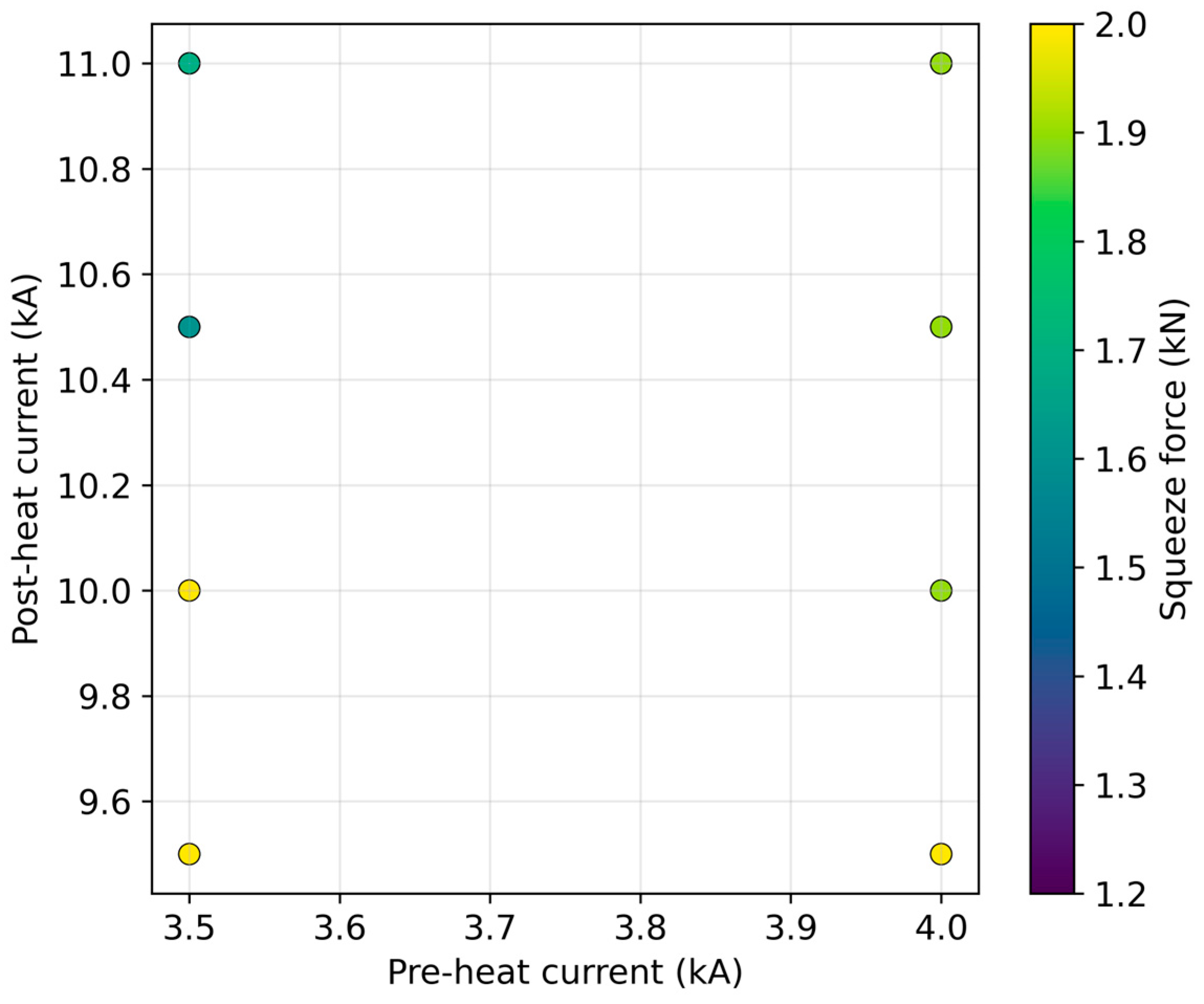
These schedules exhibit a clear trade-off between heat input, and squeeze force. In the weld current map (Figure 8), the RF-screened schedules occur only at pre-heat currents of 3.5 and 4.0 kA, while the post-heat current ranges from 9.5 to 11.0 kA. The color distribution indicates that schedules at lower post-heat currents generally require higher squeeze force, whereas schedules at higher post-heat currents can remain feasible over a wider range of squeeze forces. This finding confirms that the required upset is governed not by current alone, but by the combined balance between Joule heating and squeeze force.

Figure 8. Weld current map for RF-screened schedules.

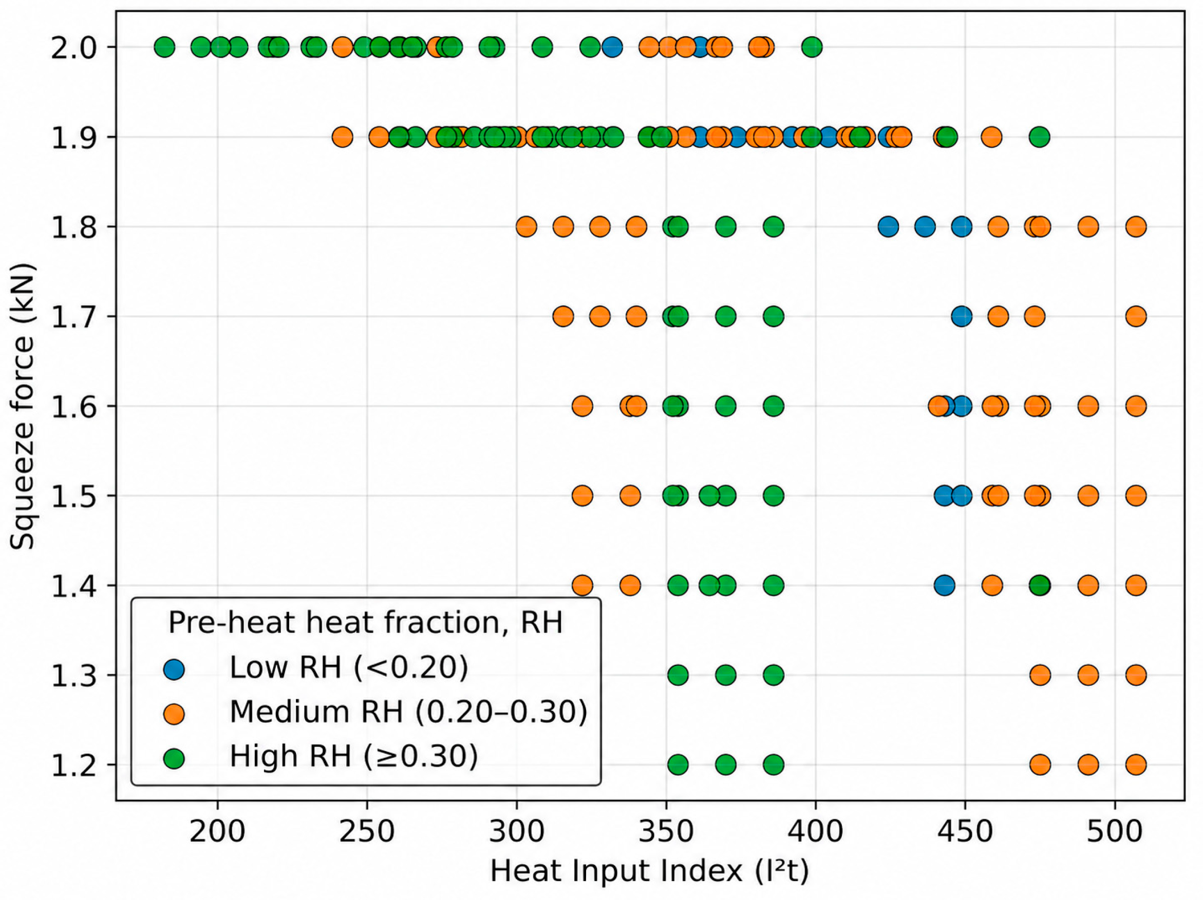
To further interpret the thermo-mechanical basis of these schedules, electrical heat input represented by the I²t-based Heat Input Index (HII) and pre-heat heat fraction (RH) representing fraction of the input given in pre-heat stage are introduced.

$$\mathrm{H}\mathrm{I}\mathrm{I}=I_{pre}^2{t}_{pre}+I_{post}^2{t}_{post}$$

(2)

$$\mathrm{R}\mathrm{H}={\displaystyle \frac{I_{pre}^{2}t}{I_{pre}^{2}t+I_{post}^{2}t}}$$

(3)

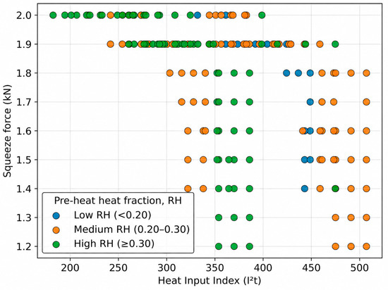
The Heat Input Index–squeeze force map (Figure 9) provides a compact mechanistic interpretation by combining the total thermal input with its distribution between the pre-heating and post-heating stages.

Figure 9. Heat Input Index–squeeze force map.

The RF-screened schedules occupy a wide HII range, indicating that the target upset can be achieved through multiple combinations of current and heating duration. At lower HII values, the schedules are concentrated mainly at high squeeze forces of 1.9–2.0 kN, indicating that limited Joule heating must be compensated by a higher squeeze force to promote interfacial contact and plastic flow. As HII increases, the RF-screened schedules extend toward lower squeeze forces because greater thermal softening reduces the external force required to achieve the specified upset. The color-coded pre-heat heat fraction further shows that most schedules fall within medium and high pre-heat heat-fraction regimes, indicating that adequate thermal conditioning during the pre-heat stage is important for stabilizing subsequent post-heat deformation. Low pre-heat heat-fraction schedules are comparatively fewer and occur mainly at higher HII values, suggesting that when the pre-heating contribution is small, higher total heat input from post-heating is required to compensate. Overall, Figure 9 shows that the target upset is governed by a coupled balance among total heat input, heat partitioning between welding stages, and squeeze force, rather than by any single process variable.

Representative welding schedules selected from the screened schedules were experimentally evaluated to verify the RF predictions. The close agreement between RF-predicted and measured upset values (Table 7) supports the practical applicability of the FE–RF approach within the investigated parameter domain. Extensive experimental verification was constrained by high processing costs and limited machine availability. Accordingly, three representative welding schedules spanning the investigated parameter range were selected for experimental verification of the FE–RF approach.

Table 7. Experimental verification of RF-model-predicted weld schedules.

SN	Input Parameters					Output Parameters
	Pre-Heat Current (kA)	Post-Heat Current (kA)	Squeeze Force (kN)	Pre-Heat Time (Cycles)	Post-Heat Time (Cycles)	Pre-Heat Upset (mm)		Total Upset (mm)
						E 1	M 1	E 1	M 1
1	4	11	1.6	7	2	0.62	0.59	1.15	1.13
2	4	11	1.2	7	2	0.55	0.58	1.12	1.10
3	3.5	9.5	2	9	3	0.6	0.59	1.2	1.2

¹ E: Experimental, M: RF prediction.

4. Conclusions

• Experimentally validated FE simulations were used to generate the dataset for RF prediction of pre-heat and total upset in multi-cycle resistance end-closure welding of Zr-4 fuel elements.
• The optimized RF models achieved independent blind-test RMSEs of 0.06 mm and 0.08 mm for pre-heat upset and total upset, respectively, demonstrating engineering -level predictive accuracy. Ten-seed evaluation and learning-curve convergence demonstrated stable regression performance within the investigated parameter domain.
• RF-assisted full-factorial screening of 4725 combinations identified 176 candidate schedules whose predicted responses satisfied both target upset ranges. Analysis of these schedules revealed a thermo-mechanical trade-off among electrical heat input, heat partitioning, and squeeze force rather than a unique welding schedule.
• The proposed FE–RF approach enables rapid process space screening and production-oriented weld-schedule development while substantially reducing the need for repeated FE simulations and welding trials.

References

- Banerjee, S. Nuclear Materials: Metallurgy and Properties of Nuclear Fuels; CRC Press: Boca Raton, FL, USA, 2011. [Google Scholar]
- Setty, D.S.; Kapoor, K.; Saibaba, N. Nuclear fuel cycle - developments and challenges in fuel fabrication technology in India. Prog. Nucl. Energy 2017, 101, 100–117. [Google Scholar] [CrossRef] [Scilit]
- Lemaignan, C.; Motta, A.T. Zirconium Alloys in Nuclear Applications. In Materials Science and Technology; Cahn, R.W., Haasen, P., Kramer, E.J., Eds.; Wiley-VCH: Weinheim, Germany, 2006. [Google Scholar] [CrossRef] [Scilit]
- Ganguly, C. Advances in zirconium Technology for Nuclear Reactor Applications. In Proceedings of the Symposium Zirconium, ZIRC; Bhabha Atomic Research Centre: Mumbai, India, 2002; pp. 1–27. [Google Scholar]
- Kim, S.-S.; Koh, J.-H.; Lee, J.-W.; Park, G.-I. Application of Welding Technology for a Zirconium Alloy of Nuclear Fuel Cladding. J. Korean Weld. Join. Soc. 2011, 29, 5–8. [Google Scholar] [CrossRef] [Scilit]
- Slobodyan, M. Resistance, electron- and laser-beam welding of zirconium alloys for nuclear applications: A review. Nucl. Eng. Technol. 2021, 53, 1049–1078. [Google Scholar] [CrossRef] [Scilit]
- Setty, D.S.; Ravinder, R.P.; Murthy, A.L.N. Resistance butt welding of zirconium alloy material. Mater. Manuf. Process. 2008, 23, 844–851. [Google Scholar] [CrossRef] [Scilit]
- Mabrouki, M.; Gonçalves, D.; Pascal, S.; Bertheau, D.; Henaff, G.; Poulon-Quintin, A. Optimization of the Pressure Resistance Welding Process for Nuclear Fuel Cladding Coupling Experimental and Numerical Approaches. Metals 2023, 13, 291. [Google Scholar] [CrossRef] [Scilit]
- Lindgren, L.E. Finite Element Modeling and Simulation of Welding Part 1: Increased Complexity. J. Therm. Stress. 2001, 24, 141–192. [Google Scholar] [CrossRef] [Scilit]
- Tsirkas, S.A.; Papanikos, P.; Kermanidis, T. Numerical Simulation of the Laser Welding Process in Butt-Joint Specimens. J. Mater. Process. Technol. 2003, 134, 59–69. [Google Scholar] [CrossRef] [Scilit]
- Na, T.H. Simulation-Based Characterization of Tube-Cap Resistance Butt Welding of Nuclear Fuel for Light Water Reactors and Development of Melted-Volume Prediction Models. Int. J. Precis. Eng. Manuf. 2023, 24, 1443–1451. [Google Scholar] [CrossRef] [Scilit]
- Nielsen, C.V.; Martins, P.A.F.; Zhang, W.; Bay, N. Numerical Methods in Simulation of Resistance Welding. In Proceedings of the VI International Conference on Coupled Problems in Science and Engineering, Venice, Italy, 18–20 May 2015. [Google Scholar]
- Mackerle, J. Finite element analysis and simulation of welding: A bibliography (1976–1996). Model. Simul. Mater. Sci. Eng. 1996, 4, 501. [Google Scholar] [CrossRef] [Scilit]
- Trupiano, S.; Belardi, V.G.; Fanelli, P.; Gaetani, L.; Vivio, F. A novel modeling approach for multi-passes butt-welded plates. J. Therm. Stress. 2021, 44, 829–849. [Google Scholar] [CrossRef] [Scilit]
- Pu, X.; Zhang, C.; Li, S.; Deng, D. Simulating welding residual stress and deformation in a multi-pass butt-welded joint considering balance between computing time and prediction accuracy. Int. J. Adv. Manuf. Technol. 2017, 93, 2215–2226. [Google Scholar] [CrossRef] [Scilit]
- Lindgren, L.-E. Numerical modelling of welding. Comput. Methods Appl. Mech. Eng. 2006, 195, 6710–6736. [Google Scholar] [CrossRef] [Scilit]
- Murakawa, H.; Oda, I.; Itoh, S.; Serizawa, H.; Shibahara, M.; Nishikawa, H. Iterative substructure method for fast FEM analysis of mechanical problems in welding. In Preprints of the National Meeting of JWS; Japan Welding Society: Tokyo, Japan, 2004; Volume 75, pp. 274–275. [Google Scholar]
- Barsoum, Z.; Bhatti, A.A.; Balawi, S. Computational Weld Mechanics—Towards a Simplified and Cost Effective Approach for Large Welded Structures. Procedia Eng. 2015, 114, 62–69. [Google Scholar] [CrossRef] [Scilit]
- Wuest, T.; Weimer, D.; Irgens, C.; Thoben, K.D. Machine learning in manufacturing: Advantages, challenges, and applications. Prod. Manuf. Res. 2016, 4, 23–45. [Google Scholar] [CrossRef] [Scilit]
- Tercan, H.; Meisen, T. Machine learning and deep learning based predictive quality in manufacturing: A systematic review. J. Intell. Manuf. 2022, 33, 1879–1905. [Google Scholar] [CrossRef] [Scilit]
- Asif, K.; Zhang, L.; Derrible, S.; Indacochea, J.E.; Ozevin, D.; Ziebart, B. Machine learning model to predict welding quality using air-coupled acoustic emission and weld inputs. J. Intell. Manuf. 2022, 33, 881–895. [Google Scholar] [CrossRef] [Scilit]
- Wang, P.E.; Ghassemi-Armaki, H.; Pour, M.; Zhao, X.; Ma, J.; Sattari, K.; Carlson, B. Applicable and generalizable machine learning for intelligent welding in automotive manufacturing. Weld. World 2025, 69, 1349–1384. [Google Scholar] [CrossRef] [Scilit]
- He, Y.; Yang, K.; Wang, X.; Huang, H.; Chen, J. Quality Prediction and Parameter Optimisation of Resistance Spot Welding Using Machine Learning. Appl. Sci. 2022, 12, 9625. [Google Scholar] [CrossRef] [Scilit]
- Zhang, M.; Xu, X.; Polzer, J.; Liu, Q.; Chen, X.; Chen, X. Data-driven artificial intelligence methods for real-time welding defect diagnosis: A critical review and future outlook. J. Manuf. Process. 2026, 161, 49–63. [Google Scholar] [CrossRef] [Scilit]
- Sun, J.; Deng, J.; Peng, W.; Zhang, D. Strip Crown Prediction in Hot Rolling Process Using Random Forest. Int. J. Precis. Eng. Manuf. 2021, 22, 301–311. [Google Scholar] [CrossRef] [Scilit]
- Dogan, A.; Birant, D. Machine learning and data mining in manufacturing. Expert Syst. Appl. 2021, 166, 114060. [Google Scholar] [CrossRef] [Scilit]
- Domínguez-Molina, L.A.; Rivas-Araiza, E.; Jauregui-Correa, J.C.; Gonzalez-Cordoba, J.L.; Pedraza-Ortega, J.C.; Takacs, A. Resistance Welding Quality Through Artificial Intelligence Techniques. Sensors 2025, 25, 1744. [Google Scholar] [CrossRef] [Scilit]
- Jeong, Y.; Wang, Y.; Truong, V.D.; Jang, S.; Lee, J.; Yoon, J. Ensemble machine learning model for prediction of inner welding defects in orbital GTAW (Gas Tungsten Arc Welding) process with monitored by multi-sensor system. Int. J. Press. Vessel. Pip. 2025, 218, 105632. [Google Scholar] [CrossRef] [Scilit]
- Feng, G.; Lin, J.; Yang, J.; Liang, Z.; Lu, L.; Lei, Y.; Fu, H. Numerical modeling of pressure resistance welding of zirconium alloy tube-end plug joint. Int. J. Adv. Manuf. Technol. 2022, 121, 3337–3350. [Google Scholar] [CrossRef] [Scilit]
- Na, T.H.; Lee, B.H.; Kim, M.W.; Na, S.J. Quality monitoring of end plug resistance weldment for nuclear fuel rods by electrode displacement. Int. J. Adv. Manuf. Technol. 2018, 99, 2509–2522. [Google Scholar] [CrossRef] [Scilit]
- Zhang, W. Design and implementation of software for resistance welding process simulations. Trans. J. Mater. Manuf. 2003, 112, 556–564. [Google Scholar]
- Feith, A.D. Thermal Conductivity and Electrical Resistivity of Zircaloy-4; Nuclear systems programs; GEMP–869; General Electric Company: Cincinnati, OH, USA, 1965. [Google Scholar]
- Rivera, J.E. Performance of Light Water Reactor Fuel Rods During Plant Power Changes. Doctoral Dissertation, Massachusetts Institute of Technology, Cambridge, MA, USA, January 1981. [Google Scholar]
- MacDonald, P.E.; Thompson, L.B. MATPRO—A Hand Book of Material Properties for Use in the Analysis of Light Water Reactor Fuel Rod Behavior; SEE CODE-9502158; Aerojet Nuclear Co.: Idaho Falls, ID, USA, 1976. [Google Scholar]
- International Atomic Energy Agency. Thermophysical Properties Database of Materials for Light Water Reactors and Heavy Water Reactors; IAEA-TECDOC-1496; IAEA: Vienna, Austria, 2006. [Google Scholar]
- McKay, M.D.; Beckman, R.J.; Conover, W.J. A Comparison of Three Methods for Selecting Values of Input Variables in the Analysis of Output from a Computer Code. Technometrics 1979, 21, 239–245. [Google Scholar] [CrossRef] [Scilit]
- Montgomery, D.C. Design and Analysis of Experiments, 10th ed.; Wiley: Hoboken, NJ, USA, 2019. [Google Scholar]
- Taguchi, G. Introduction to Quality Engineering: Designing Quality into Products and Processes; Asian Productivity Organization: Tokyo, Japan, 1986. [Google Scholar]
- Roy, R.K. A Primer on the Taguchi Method, 2nd ed.; Society of Manufacturing Engineers: Southfield, MI, USA, 2010. [Google Scholar]
- Breiman, L. Random Forests. Mach. Learn. 2001, 45, 5–32. [Google Scholar] [CrossRef] [Scilit]
- Kohavi, R. A study of cross-validation and bootstrap for accuracy estimation and model selection. In Proceedings of the 14th International Joint Conference on Artificial Intelligence—Volume 2 (IJCAI’95); Stanford University: Stanford, CA, USA, 1995; Volume 2, pp. 1137–1143. [Google Scholar]
- Arlot, S.; Celisse, A. A survey of cross-validation procedures for model selection. Stat. Surv. 2010, 4, 40–79. [Google Scholar] [CrossRef] [Scilit]
- Probst, P.; Wright, M.N.; Boulesteix, A.-L. Hyperparameters and tuning strategies for random forest. WIREs Data Min. Knowl. Discov. 2019, 9, e1301. [Google Scholar] [CrossRef] [Scilit]
- Bergstra, J.; Bengio, Y. Random search for hyper-parameter optimization. J. Mach. Learn. Res. 2012, 13, 281–305. [Google Scholar]
Disclaimer/Publisher’s Note: The statements, opinions and data contained in all publications are solely those of the individual author(s) and contributor(s) and not of MDPI and/or the editor(s). MDPI and/or the editor(s) disclaim responsibility for any injury to people or property resulting from any ideas, methods, instructions or products referred to in the content. |
© 2026 by the authors. Licensee MDPI, Basel, Switzerland. This article is an open access article distributed under the terms and conditions of the Creative Commons Attribution (CC BY) license.