From the Phase Dynamics of Synchronization and Elliptical Gears to a Semiclassical Model of Zitterbewegung with Spin-like Properties

Abstract

The spin of an electron is an intrinsic quantum property that cannot be explained using classical mechanics. Nevertheless, it is possible to conceive semiclassical systems with internal degrees of freedom that exhibit spin-like properties. Building on the analysis of phase modulation by elliptical gears and kinematically equivalent antiparallelogram linkages, we present a novel semiclassical model of Zitterbewegung, a rapid oscillatory motion closely connected with spin. The kinematical analog is based on including the internal rotation of the linkage represented in spacetime. The system’s dynamics is related to two-center electron models, which describe the constant momentum of the center of mass and the lightlike oscillation of the center of charge at twice the Compton frequency for a particle at rest. A two-dimensional extension provides an intuitive illustration of topological spin properties and can be used to calculate the spin and magnetic moment of an electron.

1. Introduction

The spin of an electron is a fundamental and genuine quantum property. Pauli, who was central in developing the quantum theory of spin, characterized its properties as “classically non-describable two-valuedness” [1]. Dirac, whose equation provided a fully relativistic theory of electron spin, also addressed the failure of classical models, albeit in a more detailed way. He pointed out that spin should be pictured as resulting from some internal motion of the particle, based on degrees of freedom different from those describing the particle as a whole. He concluded that “The spin does not correspond very closely to anything in classical mechanics, so the method of classical analogy is not suitable for studying it” [2].

The idea of visualizing spin-like properties of a classical object connected to a fixed frame by long, flexible strings goes back to Dirac himself [3]. His string and scissor demonstration shows that such a tethered mechanical object requires two full rotations to return the entire system, including the strings, to its initial state. The same applies to the state of an electron in Hilbert space, which must be rotated by $4\pi$ before the initial value of its complex wave function is restored. Thus, the string model does not represent a close analogy, but rather a more abstract correspondence. It visualizes the inherent topological properties of complex-valued spin vectors (spinors), which transform to their negative value after a $2\pi$ rotation. A Möbius strip is the most prominent topological spinor model that illustrates this behavior.

This paper presents a novel cogwheel-type mechanical model with internal degrees of freedom that exhibit oscillatory properties associated with spin-like behavior. Based on elliptical gears and the internal kinematics of the associated antiparallelogram linkage [4], this system was originally designed to extend the scope of existing mechanical models of phase modulation for synchronization [5]. The dynamics of the reduced phase is represented by the phase angle of the rotating ellipses. Additionally, an extended model includes linear propagation. This establishes a connection between phase and gear-driven motion consistent with the energy-momentum relation of a relativistic particle.

We show that reducing the kinematics of the linkage to a two-center description in spacetime yields close analogies with two-center electron models, reproducing the timelike propagation of the center of mass (CM) and lightlike oscillation of the center of charge (CC) in the highly relativistic limit. The latter corresponds to Zitterbewegung, a German term coined by Schrödinger [6] that means meaning ‘jittery motion’. We use the abbreviation ZBW. The relativistic Dirac equation theoretically predicts this rapid internal oscillation of an electron at twice the Compton frequency, which is closely connected to electron spin. The present model is quasi- or semiclassical because it reinterprets the phase of oscillators using relativistic and quantum correspondences. This redefines Euclidean variables in terms of Minkowski spacetime. Therefore, the analogies are consistent with the caveat that spin does not entirely reflect the internal dynamics of any classical model.

The article is divided into two main sections that differ in the dimensionality of their underlying models. The first part considers the one-dimensional propagation of the planar gear model along the sinusoidal pitch line. After providing an overview of previous results and summarizing their relativistic and quantum correspondences, the kinematics of the associated antiparallelogram linkage is analyzed using a two-center model. Although the amplitude match is perfect, a purely sinusoidal oscillation that agrees with the predictions from the Dirac equation is obtained only in the highly relativistic case. This limitation is overcome by incorporating rotations in the $x,y$-plane, transforming the planar model into a $(1+2)$-dimensional system with one time coordinate and two spatial coordinates. This provides an analog semiclassical description of the electron’s spin and magnetic moment. The concluding sections evaluate the potential and limitations of the approach, as well as its ontological and educational implications.

2. Synchronization, Phase Modulation and Linear Propagation Driven by Elliptical Gears: A Summary of Analytical Models

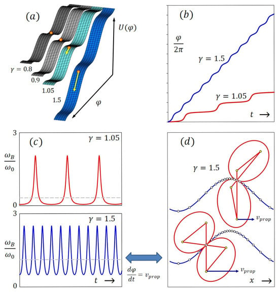
To lay the theoretical groundwork for the spin analogy, we briefly review the exact correspondence between the phase model of synchronization and linear motion driven by elliptical gears (see [4] for a detailed description). Figure 1 provides a visual summary of the parallels, illustrating the core ideas. Synchronization is a universal phenomenon in driven or coupled self-sustaining oscillators, resulting in locking to a common frequency despite the oscillators’ different natural frequencies. It depends on essential nonlinearities that underlie the transition from phase locking to incomplete synchronization, characterized by periodic phase modulation. In a strongly reduced model, the phase of a self-oscillator under weak sinusoidal driving is described by the Adler equation [7]. More information on the history of this equation and its relation to the Kuramoto model, as well as a description of mechanical models, can be found in [5]. The Adler equation in dimensionless time $\tau$ reads.

$${\displaystyle \frac{d\phi }{d\tau }}=\gamma -\mathit{sin}\phi .$$

(1)

$\phi$ is the phase difference between the oscillator and the drive signal. The factor $\gamma =(\omega -{\omega }_D)/{\omega }_{0 }$ describes the relative detuning of the frequency difference $\omega {-\omega }_D$ between the instantaneous oscillator frequency $\omega$ and the drive frequency ${\omega }_D$ with respect to a critical frequency ${\omega }_{0 }$, which is identical to the eigenfrequency of the self-oscillator. Lab time is $t=\tau /{\omega }_0$. For simplicity we omit the term angular throughout the article. ${\omega }_{0 }$is always chosen as one cycle per unit time.

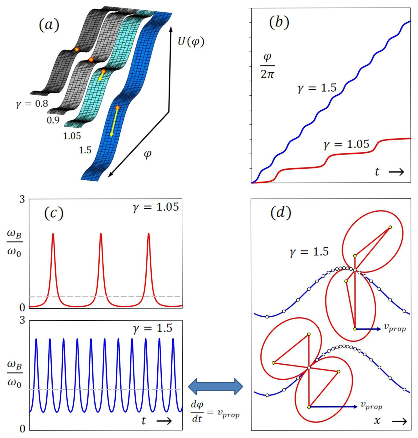
Figure 1. Visual summary of the correspondence between synchronization and linear propagation driven by elliptical gears. The tilted washboard potential in (a) illustrates the $\gamma$-dependent transition from phase locking to running phase solutions. Diagrams (b,c) depict the time-dependent phase $\phi \left(t\right)$, and the corresponding phase rate $d\phi /dt={\omega }_B\left(t\right)$, normalized to ${\omega }_B/{\omega }_0$. Diagram (d) shows two snapshots, taken half a period apart, of the ellipses propagating along the stationary pitch line. See the text for details.

Without solving the equation explicitly, a potential energy landscape resembling a tilted washboard, given by $U\left(\phi \right)=-\gamma \phi -\mathit{cos}\phi$, illustrates the dynamics. The inclination $-dU/d\phi$ is corresponds to the phase rate $d\phi /d\tau$. It describes the motion of a ‘phase particle’, sliding down an inclined plane with sinusoidal corrugations under the influence of strong velocity-proportional friction. Figure 1a sketches the potential energy landscape for four different values of $\gamma$. For $\gamma <1$, the phase particle is trapped in a local minimum describing phase locking. For $\gamma >1$, running phase solutions are obtained. The average phase rate is indicated by the yellow vector.

Both phase modulation and elliptical gear kinematics underlie an Adler-type differential equation. To represent phase modulation mechanically by the kinematics of elliptical gears, it is more advantageous to modify the Adler equation by replacing the sine by cosine, with a positive or negative sign, depending on the context. Apart from phase shifts, the resulting dynamics is equivalent. This modified equation is referred to as Adler-type to distinguish it from the original sine form. After variable separation the integral $\int {\displaystyle \frac{d\phi }{\gamma \pm \mathit{cos}\phi }}={\omega }_{0}t+C$ is obtained, which can be solved analytically as shown in [4]. We only consider running phase solutions for positive detuning ($\gamma$ > 1).

With a negative cosine term, the phase angle with the initial condition $\phi \left(0\right)=0$ is given by

$$\phi (t)=2{\mathit{tan}}^{-1}\left[{\displaystyle \frac{\gamma -1}{\sqrt{{\gamma }^2-1}}}\mathit{tan}\left({\displaystyle \frac{\sqrt{{\gamma }^2-1}}{2}}{\omega }_{0}t\right)\right].$$

(2)

For a positive cosine term, replace the factor in the square bracket by $(\gamma +1)/\sqrt{{\gamma }^2-1}$. Phase modulation leads to a periodically varying phase rate, which corresponds to the instantaneous beat frequency ${\omega }_B$:

$${\omega }_B\left(t\right)={\displaystyle \frac{d\phi }{dt}}={\displaystyle \frac{\left({\gamma }^2-1\right){ \omega }_0}{\gamma +\mathit{cos}\left(\sqrt{\left({\gamma }^2-1\right)}{ \omega }_{0}t\right)}}.$$

(3)

Figure 1b shows the nonlinear increase in phase for two values of $\gamma$. Figure 1c displays the corresponding instantaneous beat frequencies ${\omega }_B\left(t\right)$. The respective time averages $⟨{\omega }_B⟩=\sqrt{\left({\gamma }^2-1\right)}{\omega }_0$ are indicated by the gray dotted lines.

To connect phase modulation with gear-driven propagation, consider an elliptical gear arrangement with an upright rack that fixes the rotation centers in the foci of each ellipse vertically, while the two rotating ellipses in mechanical contact propagate horizontally along a sinusoidal pitch curve described by their contact point (Figure 1d).

In order to achieve a match between phase and the covered distance, the semi-major axis $A$ of the ellipses is set to $A=\gamma$, with linear eccentricity $C=1$. This yields $e=1/\gamma$ for the numerical eccentricity and $B=\sqrt{{\gamma }^2-1}$ for the semi-minor axis (all lengths and distances in dimensionless units). The dimensions of the associated antiparallelogram linkage are given accordingly. The long bars of the linkage are $2A$ in length. The length of the rotating short bars is set to twice the linear eccentricity. The pitch curve equation is $y=\gamma -\cos \theta$, where $\theta =x/B$.

Figure 1d shows two snapshots of the system. The contact point of the counter-rotating ellipses moves along the sinusoidal pitch curve while oscillating along the co-moving vertical rack. With the upper driving ellipse in uniform rotation at a phase angle ${\phi }_1=\sqrt{\left({\gamma }^2-1\right)}{\omega }_{0}t$, the rack position is given by [8]:

$$x(t)=2\sqrt{{\gamma }^2-1}{\mathit{tan}}^{-1}\left[{\displaystyle \frac{\gamma +1}{\sqrt{{\gamma }^2-1}}}\mathit{tan}\left({\displaystyle \frac{{\phi }_1}{2}}\right)\right].$$

(4)

The propagation velocity is not uniform, as indicated by the small circular marks that are equidistant in time.

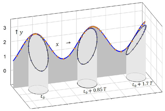
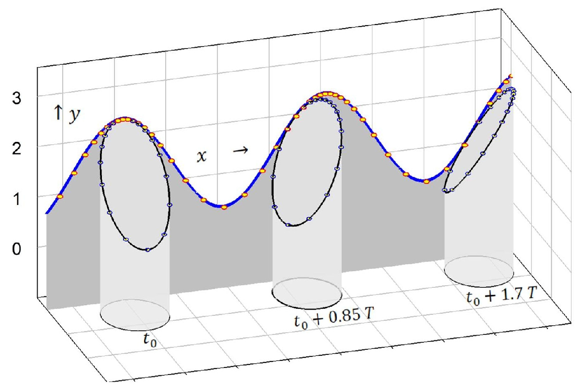
In one period, the rack travels $2\pi B$, which is the distance covered by a cylinder of radius $B$ rolling along the $x$-axis. The rolling cylinder, equipped with an oblique cut, provides an alternative visualization of the elliptical gear driven propagation. The cylinder’s oblique cut is elliptical. The contact point between the elliptical edge and the planar surface along which the cylinder rolls, traces out a sine curve [9]. Mathematically, this is based on the fact that the perimeter of an ellipse and the arc length of a sine curve are equal to the same incomplete elliptical integral of the second kind [10].

Figure 2 shows the propagation of the rotating cylinder, the phase angle of which is given by Equation (2). The resulting sine curve, described by the elliptical cut, corresponds to the pitch line in Figure 1d. The time marks and the resulting periodically modulated propagation velocity are also identical. This is an alternative visualization of the propagating gear system. Remarkably, despite being based on elliptical integrals that cannot be expressed in terms of elementary functions, this geometry is intriguingly simple yet effective in conveying the basic ideas.

Figure 2. The contact point between a plane and the elliptical cut of a rolling cylinder of radius $B=\sqrt{{\gamma }^2-1}$ describes a sine curve. By choosing a cut angle of $\theta ={\mathit{tan}}^{-1}(C/B)$, the semi-major axis of the cut becomes $\mathrm{A}=\mathsf{\gamma }$, and the shape of the elliptical cut corresponds to the counter-rotating ellipses. With $\gamma =1.5$, the pitch curve and the periodically modulated propagation velocity are identical to those in Figure 1d.

In summary, the gear model converts phase modulation into linear motion with proper velocity, a concept closely related to relativistic momentum, as shown below. This interpretation requires the inclusion of relativistic and quantum correspondences as well as the parallels between $\gamma$ interpreted as frequency boost that increases the oscillator frequency with respect to a reference level. In the quantum analogy, this corresponds to an energy boost described by the Lorentz factor $\gamma$.

3. The Integration of Relativistic and Quantum Correspondences: Extending the Model Beyond Classical Mechanics

3.1. Defining Proper Time and Coordinate Time in a Two-Clock and One-Map Approach

The model is based on a one-map and two-clock approach to special relativity [11]. It uses two different notions of time to describe positions in a common coordinate frame. Proper time is measured by an ideal clock attached to a particle, moving along a timelike world line. Coordinate time, on the other hand, is measured by a clock carried by an inertial observer who defines simultaneity of events. It is important not to confuse the symbols, since relativity textbooks use the letter $\tau$ for proper time and $t$ for coordinate time. The lab time $t$ used in the foregoing derivations is internal to the system whose timelike dynamics it describes. Therefore, it corresponds to proper time $\tau$. Most textbook problems assume that the proper time is given. In the present dynamical descriptions, however, the situation is reversed. We know the proper time, which is the lab time t in Equations (2) and (3). Thus, we must calculate the resulting coordinate time from the underlying dynamics.

To maintain consistency with the previous formulae, we keep the letter $t$ to denote proper time and introduce $t_{co}$ to denote coordinate time. Starting from the given proper time interval $∆t\equiv ∆\tau$, we derive the coordinate time interval $∆t_{co}$ to describe the motion from the perspective of an inertial frame. In special relativity the following differential relation between coordinate time and proper time holds [12]:

$$∆t_{co}=\gamma ∆t, \gamma ={\displaystyle \frac{1}{1-v^2/c^2}}= {\displaystyle \frac{1}{1-{\beta }^2}}.$$

(5)

The Lorentz factor $\gamma$ depends on $\beta$, the quotient of the velocity $\mathrm{v}$ in the map frame and the speed of light $\mathrm{c}$. As this relation is based on differential increments, it allows the extension of special relativity to accelerated motions with time-dependent $\gamma$, as is the case in the periodically accelerated dynamics of Figure 1d.

Next, we incorporate quantum correspondences into the classical phase modulation model. As self-oscillations can be considered clock-like self-sustaining processes, we establish the quantum correspondences of the model by linking the nonlinear dynamics of phase modulation to de Broglie’s seminal idea that particles behave like tiny clocks. This approach marked the beginning of modern quantum mechanics (QM) a century ago, culminating in the concept of matter waves.

3.2. Integrating the Wave–Particle Duality

De Broglie used relativistic kinematics to synchronize the internal oscillation of a propagating electron with an accompanying extended periodic process represented by a phase wave. Thus, he was able to generalize the wave–particle duality of photons to all elementary particles [13,14].

The concept of a phase wave can be visualized by imagining an infinitely long linear array of clocks set to oscillate in synchrony in their rest frame. The connection between the individual phases is an infinite, straight oscillating line. From the perspective of an observer moving along the array, the line appears to be periodically modulated according to the Lorentz transformation. The resulting spatial periodicity of the ‘simultaneity wave’ is the de Broglie wavelength ${\lambda }_B$. De Broglie proved that the phase of a clock moving with the velocity $v=\beta c$ stays in synchrony with the phase wave, provided that the latter propagates with superluminal speed $v_{ph}=c/\beta$. He coined the term ‘law of phase harmony’ to describe the kinematical synchronization.

Instead of using relativistic kinematics to synchronize the particle clock with an accompanying periodic field-like process, we consider the nonlinear dynamics of synchronizing self-oscillations. The local synchronization of phase is coupled to the linear propagation of the oscillator, as described by the propagating rack model in Figure 1d. We denote the particle clock frequency by ${\omega }_0$ to relate it to the critical detuning in phase modulation. Equating $E_0=m{c}^2$ and $E_0=\hslash {\omega }_0$ ($\hslash$ reduced Planck constant) identifies it as the Compton frequency ${\omega }_0=m{c}^2/\hslash$ of a particle at rest. Its Compton wavelength is ${\lambda }_C=2\pi c/{\omega }_0=h/mc$.

Including $\hslash$ expresses relative detuning in terms of energies: $\gamma =(\hslash \omega -\hslash {\omega }_D)/\hslash {\omega }_{0 }$. We define the reference energy level as $E_{ref}=\hslash {\omega }_D$. Since ${\omega }_D$ can be chosen arbitrarily, ${\omega }_D$ and $E_{ref}$ can be set to zero. This zero level defines the background drive frequency or the energy of the vacuum, against which excitations are created. Therefore, $\gamma$ represents an energy boost. Total energy $E$ is connected with rest energy $E_0$ by $E=\gamma \hslash {\omega }_0=\gamma E_0$. $\gamma =1$ is necessary to create a particle at rest, while obtaining a particle in motion requires $\gamma >1$. The excess energy is the particle’s kinetic energy $E_{kin}=E-E_0=(\gamma -1)E_0$. The relativistic dispersion relation describes how total energy is divided between rest energy and momentum$p.$

$$E=\sqrt{E_0^2+{\left(pc\right)}^2}.$$

(6)

Energy and momentum are components of the energy-momentum four-vector. As only one-dimensional motion is considered, vector notation is omitted. Dispersion encodes relativistic invariance of $E^2-{\left(pc\right)}^2$. All observers agree on the particle’s rest mass $m=E_0/c^2$, regardless of their reference frame. This can be checked by inserting total energy $E=\gamma E_0$ and relativistic momentum $p=\gamma mv=\beta \gamma mc$.

With the present choice of ${\omega }_0=2\pi /T_0$, the dispersion relation in dimensionless units becomes $\gamma =\sqrt{1+{\left(\beta \gamma \right)}^2}$. With the average beat frequency $⟨{\omega }_B⟩=\sqrt{\left({\gamma }^2-1\right)}{\omega }_0$ of the phase model written as $⟨{\omega }_B⟩=\beta \gamma {\omega }_0= \beta \gamma m{c}^2/\hslash$ the relativistic momentum can be expressed as

$$p=\gamma mv=\hslash ⟨{\omega }_B⟩/c.$$

(7)

3.3. Defining Coordinate Velocity and Proper Velocity

There are two derivatives that describe the rate of propagation in space. The term $v\gamma =p/m$ is known as the proper velocity. It is the quotient of the displacement $∆x$ measured in the coordinate frame and the proper time difference $∆t$, measured in the system in motion: $v_{prop}=∆x/∆t= \beta \gamma c$. Coordinate velocity is given by $v_{cord}=\mathsf{\Delta }x/\mathsf{\Delta }{t}_{co}$. To show that the propagation velocity of the rack travelling the distance $x\left(t\right)$ according to dimensionless Equation (4) corresponds to $v_{prop}$, the length scale must be defined. The underlying unit length C of the elliptic parameters in Figure 1 is the reduced Compton wavelength ${\mathrm{ƛ}}_{\mathrm{C}}=c/{\omega }_0$ and the radius of the propagating cylinder in Figure 2 is $r=\sqrt{{\gamma }^2-1}{\mathrm{ƛ}}_{\mathrm{C}}$. The distance covered in one period is $∆x=\sqrt{{\gamma }^2-1}·2\pi c/{\omega }_0$. The proper time unit, given by the Compton frequency, is $T_0=2\pi /{\omega }_0$. $∆x/T_0$ yields the proper velocity of the rack $v_{prop}=c\sqrt{{\gamma }^2-1}=c\beta \gamma =v\gamma$, which agrees with Equation (7).

In the full relativistic formalism, proper velocity is part of a four-vector, defined as the derivative of the position in four-dimensional spacetime with respect to proper time. The three derivatives of the spatial coordinates describe the spatial rates in proper time, and the derivative of the fourth component relates to the rate of coordinate time.

Table 1 summarizes the correspondence between the classical variables of the model and their relativistic and quantum mechanical counterparts. Note that the meaning of $\gamma$ differs on the two sides of the table; however, the two meanings are related based on the underlying correspondences. On the left-hand side, $\gamma$ describes relative detuning. It can be considered a frequency boost if the driving signal’s frequency ${ \omega }_D$ is set to zero as a reference level. Multiplying by $\hslash$ yields the relativistic energy boost factor $\gamma$ on the right-hand side, which is identical to the Lorentz factor.

Table 1. Summary of correspondences.

Phase Modulation & Elliptical Gear Model	Relativistic & QM Correspondences
relative detuning $\gamma =(\omega -{\omega }_D)/{\omega }_{0 }$ with $\mathrm{r}\mathrm{e}\mathrm{f}\mathrm{e}\mathrm{r}\mathrm{e}\mathrm{n}\mathrm{c}\mathrm{e} \mathrm{l}\mathrm{e}\mathrm{v}\mathrm{e}\mathrm{l} {\mathsf{\omega }}_{\mathrm{D}}\equiv 0$: frequency boost $\gamma =\omega /{\omega }_{0 }$	energy boost $\gamma =\hslash \omega /\hslash {\omega }_{0 }=E/E_0$ with Lorentz factor $\gamma =1/\sqrt{1-{\beta }^2}$
critical detuning ${\omega }_0$	particle at rest with $E_0=\hslash {\omega }_0$
average beat frequency $⟨{\omega }_B⟩=\sqrt{{\gamma }^2-1}{\omega }_0=\beta \gamma {\omega }_0$	average particle momentum $p=\hslash ⟨{\omega }_B⟩/c$ =$\gamma mv=\beta \gamma mc$ with average velocity $v_{coord}=\beta c$
one timescale and one velocity $t=t_{prop}$& $v_{prop }=dx/dt=\beta \gamma c$	two timescales and two velocities: $t_{prop }$& $t_{coord}=\gamma t_{prop }$ $v_{prop }$& $v_{coord}=v_{prop }/\gamma =\beta c$

Proper velocity $v_{prop}=v\gamma =p/m$ corresponds to momentum per mass. Unlike coordinate velocity, it is not bounded and can exceed the speed of light. However, the apparent superluminal propagation does not violate relativity theory, since the resulting coordinate velocity, given by $v_{coord}=∆x/∆t_{co}=\beta c$, does not exceed the speed of light. As it is not a widespread notion, it is helpful to point out that proper velocity is an important concept in spaceflight. It is the speed at which an astronaut perceives the passage of external objects [15]. In principle, astronauts travelling at extreme, yet subluminal, speeds could reach distant galaxies within their lifetime. Proper velocity has the advantage that it can be composed in the Newtonian way, without resorting to the relativistic addition of coordinate velocities.

4. Kinematics of the Two-Center Rack Model: Lemniscates and the Zitterbewegung Analogy

In Schrödinger’s analysis of ZBW, as elaborated within the framework of a two-center model of the electron, it describes a sinusoidal oscillation of the center of charge (CC) at light velocity. It oscillates at twice the Compton frequency $2{\omega }_0$ with amplitude equal to half the reduced Compton wavelength ${\mathrm{ƛ}}_{\mathrm{C}}/2=\mathbf{\hslash }/2mc=\mathrm{c}/2{\mathsf{\omega }}_0$ [16]. These oscillations superpose the motion of the system as a whole, represented by the center of mass (CM), which propagates at a constant average velocity.

Thus far, we have considered the gear-driven propagation of the vertical rack along the fixed pitch line and attributed this to the movement of the system as a whole. The antiparallelogram linkage possesses an additional internal degree of freedom, described by the center motion of the rotating crossed bar. In the reference frame of a stationary rack, it traces a figure of eight. This planar figure belongs to the lemniscate family—a famous class of mathematical objects that also includes the infinity symbol $\infty$.

In the rack model, the center of the vertical rack is identified as the CM. It propagates in $x$-direction with the proper velocity $v_{prop}$ along the pitch line. The time average corresponds to a motion with constant momentum $p=\gamma mv$. The center of the rotating crossed bar is assigned to the CC. The horizontal component, denoted by $x_{cc}$, is considered to be the semiclassical analogue of ZBW. Subsequent analyses provide a theoretical justification for this preliminary assignment.

In contrast to the results presented in Section 2, we change the model. First, we express the phase angle of rotation by the Compton frequency ${\phi =\omega }_{0}t$. This ensures that $x_{cc}$ oscillates at twice the Compton frequency, as required by ZBW. This change in frequency does not affect the conformity of rack propagation with relativistic dispersion, which is encoded in the elliptic parameters of the model.

The second change involves the modulated phase angles of the rotating ellipses, which are chosen so that the vertical rack propagates with constant proper velocity rather than undergoing periodical acceleration as in Figure 1d. This is achieved by solving the kinematical equations for ${\phi }_1\left(t\right)$ and ${\phi }_2\left(t\right)$ to ensure uniform rack propagation with proper velocity $v_{prop}=\beta \gamma c$.

According to Equation (4) the rack propagation in natural units is given by

$$x=2\beta \gamma {\mathit{tan}}^{-1}\left[{\displaystyle \frac{\gamma +1}{\beta \gamma }}\mathit{tan}\left({\displaystyle \frac{{\phi }_1}{2}}\right)\right]/{\omega }_0.$$

(8)

The distance covered at an average proper velocity is given by $x=\beta \gamma t$, also in natural units. Substituting $x$ into (8) and solving for ${\mathsf{\phi }}_{\mathrm{i}}$ yields the phase of the driving ellipse.

$${\phi }_1=2 {\mathit{tan}}^{-1}\left[\sqrt{{\displaystyle \frac{\gamma -1}{\gamma +1}}}\mathit{tan}\left({\displaystyle \frac{{\omega }_{0}t}{2}}\right)\right]=2 {\mathit{tan}}^{-1}\left[{\displaystyle \frac{\beta \gamma }{\gamma +1}}\mathit{tan}\left({\displaystyle \frac{{\omega }_{0}t}{2}}\right)\right].$$

(9)

The phase of the driven ellipse with complementary shape becomes

$${\phi }_2=-2 {\mathit{tan}}^{-1}\left[\sqrt{{\displaystyle \frac{\gamma +1}{\gamma -1}}}\mathit{tan}\left({\displaystyle \frac{{\omega }_{0}t}{2}}\right)\right]=-2 {\mathit{tan}}^{-1}\left[{\displaystyle \frac{\beta \gamma }{\gamma -1}}\mathit{tan}\left({\displaystyle \frac{{\omega }_{0}t}{2}}\right)\right].$$

(10)

Given the major axis $A=\gamma$, the positions of the rotating foci of ellipses 1 and 2 are ${(x}_1,y_1)=(2C\sin {\phi }_1,2C\cos {\phi }_1+2\gamma )$ and ${(x}_2,y_2)=2C(\sin {\phi }_2, \cos {\phi }_2)$. From this, the trajectory of the crossed bar’s center at ${x={(x}_1+x}_2)/2$ and $y={{(y}_1+y}_2)/2$ is calculated.

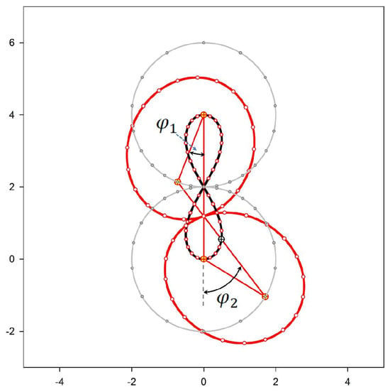
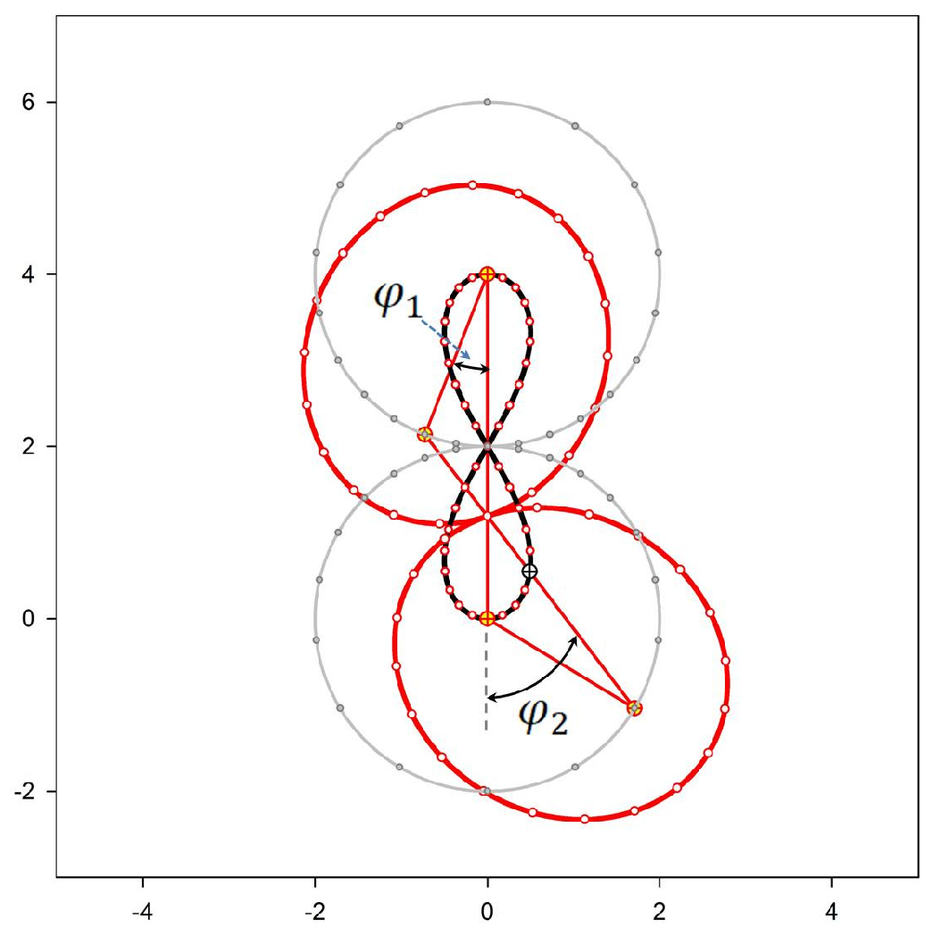
Figure 3 illustrates the lemniscate-like motion of the antiparallelogram linkage, as seen by an observer co-moving with $v_{prop}$. The upper ellipse rotates clockwise by ${\phi }_1$ around the focus fixed at $\left({xfo}_1,{yfo}_1\right)=(0,2A)$. The lower ellipse rotates by ${\phi }_2$ in the opposite direction around the focus fixed at $\left({xfo}_2,{yfo}_2\right)=(0,0)$. The radius of rotation between the fixed and the rotating focus is $2C$.

Figure 3. The center of the crossed bar, marked by $\oplus$, traces out the black lemniscate. The geometry with a fixed vertical long bar of the rack for $\gamma$ = 1.5 is shown. The two grey circles illustrate the rotation of the elliptical foci around the fixed foci. The upper driving ellipse rotates at the angle ${\phi }_1$ in clockwise direction. The driven ellipse with the angle ${\phi }_2$ rotates in opposite direction. The dots, which are equidistant in time, indicate periodically varying rotation rates.

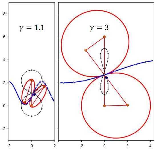
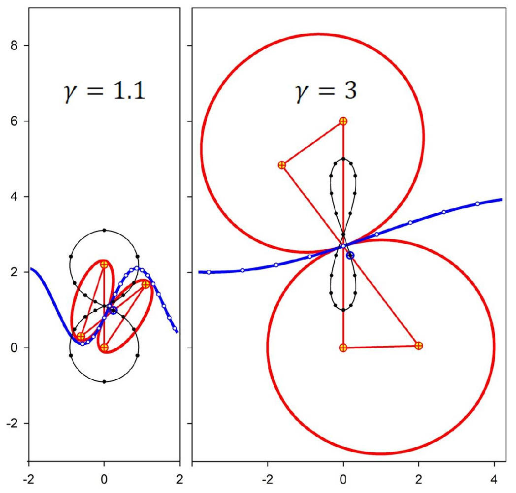
The two following figures address the $\gamma$-dependence. Figure 4 displays the lemniscates for propagating elliptical gears that roll without slipping along the pitch line $y=\gamma -\cos x/\sqrt{{\gamma }^2-1}$. Snapshots for two different values of $\gamma$ and for the same phase along the pitch curve are shown. The small circles indicate equidistant time steps. Note that, from the perspective of a co-moving observer, the vertical rack is fixed and the pitch line shifts to the left as time increases. A presentation of different lemniscate shapes and their relation to the lemniscate family is summarized in Figure 5.

Figure 4. Rotation of ellipses and the associated antiparallelogram linkage (red) combined with the CC-lemniscate (black) and pitch line propagation (blue) for $\gamma =1.4$ and $\gamma =2.5$. The perspective of an observer co-moving with $v_{prop}$ is shown. The vertical rack remains fixed, while the pitch line shifts to the left at constant time intervals, as indicated by the circular marks.

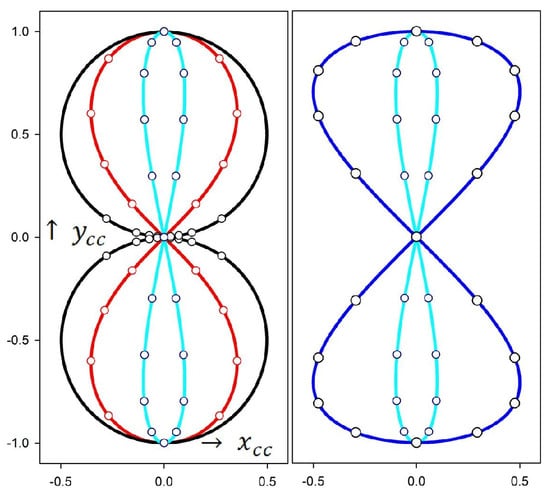
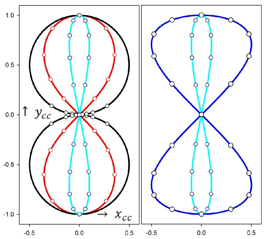
Figure 5. Different lemniscates traced out by the center of the crossed bar of the antiparallelogram linkage. The black curve on the left, for $\gamma =1.005$, represents an almost circular figure of eight with a radius approaching half unit length. The red curve for $\gamma =\sqrt{2}$ is the lemniscate of Bernoulli. The cyan curve corresponds to $\gamma =5$. Its maximum $x$-amplitude shrinks to $1/5$ of the unit radius. After scaling $x$ by the boost factor $\gamma$, it approaches the lemniscate of Gerono, shown in blue in the figure on the right. Note that the scaling in this graph is in units of the reduced Compton wavelength ${\mathrm{ƛ}}_{\mathrm{C}}$ (see text for details).

For $\gamma \to 1$, the ellipses become singular and degenerate into straight lines. The lemniscates converge to a figure of eight composed of two circles approaching unit radius $r\to C$. As $\gamma$ increases, the lemniscate $x$-amplitude decreases due to Lorentz contraction, proportional to $1/\gamma$. At $\gamma =\sqrt{2}$, the center of the crossed bar traces out the lemniscate of Bernoulli (red curve), a figure of eight found in many mathematical applications [17]. With $u={\omega }_{0}t$, this curve is parametrized by $x\left(u\right)=\sin u\cos u/\left(1+{\sin }^{2}u\right)$ and $y\left(u\right)=\cos u/\left(1+{\sin }^{2}u\right)$, with $0\le u\le 2\pi$. $\gamma =\sqrt{2}$ is also a special parameter for matter waves, because, at this value, $\beta \gamma$ = 1 and the de Broglie wavelength ${\lambda }_B$ is equal to the Compton wavelength ${\lambda }_C$. At $\gamma =5$ (blue curve), the maximum elongation in $x$-direction shrinks to $1/5$. In the case of highly relativistic boosts, multiplying the $x$-coordinate by $\gamma$ approximates another well-known planar curve: the lemniscate of Gerono, shown in blue. This curve is given by $x\left(u\right)=1/2\sin 2u$ and $y\left(u\right)=\sin u$. The continuous transformation of the Bernoulli lemniscate into an approximately circular figure eight or a squeezed Gerono lemniscate by varying ${\lambda }_B$ has not yet been described in the literature.

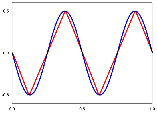
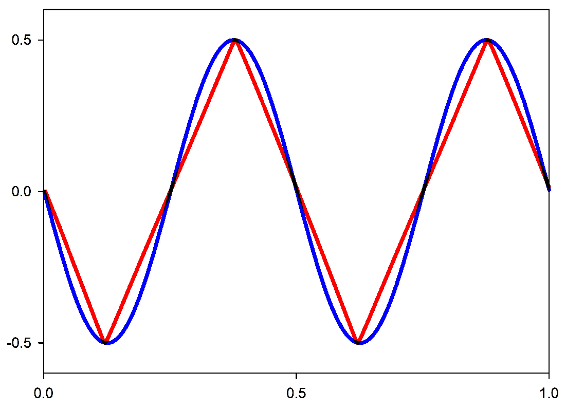
The factor $1/2$ in the $x$-coordinate matches the ZBW amplitude $\widehat{x}$ of half the reduced Compton wavelength $\widehat{x}={\mathrm{ƛ}}_{\mathrm{C}}/2=\mathbf{\hslash }/2mc=\mathrm{c}/2{\mathsf{\omega }}_0$, half the unit length of the elliptic model. With this, and the ZBW frequency of $2{\omega }_0$, the model’s lightlike CC motion is correctly predicted. This applies to a particle at rest. Note that, for a boosted particle, the frequency must be multiplied by γ, while the amplitude must be divided by γ so that the combination of energy boost and Lorentz contraction preserves the lightlike character of ZBW. However, for small values of $\gamma$, the oscillations as a function of proper time $t$ are asymmetric, as can be seen from the uneven distribution of the black time marks in the left-hand section of Figure 5. To analyze the oscillations from the common coordinate frame, proper time must be replaced by coordinate time $t_{CO}$, obtained by integrating Equation (5) as $t_{CO}=\int \gamma \left(t\right)dt$. Figure 6 shows that, as $\gamma$ approaches $1$, the XCC oscillations become triangular. This describes a zigzag motion that periodically switches speeds between $\pm c$. It is only in the highly relativistic domain that sine-shaped oscillations are approached. This is an artifact of the elliptic model, resulting in a singularity at $\gamma \to 1$.

Figure 6. XCC-oscillations in units of the reduced Compton wavelength ${\mathrm{ƛ}}_{\mathrm{C}}$ for $\gamma =1.01$ (red) and $\gamma =50$ (blue), plotted as a function of coordinate time for one period of the boosted Compton frequency $\gamma {\omega }_0$. The amplitudes are multiplied by $\gamma$ to correct for Lorentz contraction.

The issue of non-sinusoidal oscillations for $\gamma \to 1$ can be resolved by extending the model to account for rotations in the $xy$-plane. The next section will analyze the case of a particle at rest $(\gamma =1)$, using an extended model that includes uniform circular rotations.

5. Connecting Zitterbewegung and Electron Spin: Geometric Illustrations and Topological Models

5.1. From the Planar Model to Spherical Representations

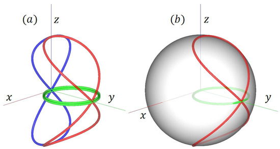
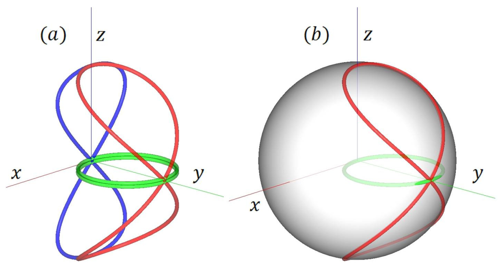
To fully elucidate the connection between ZBW and particle spin, the planar model must be extended to include rotation in the $x,y$-plane. In this case, a description in terms of rotating linkages is no longer feasible, so we must leave the context of elliptical gears. With a unit radius of $r={\mathrm{ƛ}}_{\mathrm{C}}/2$ and a unit frequency of $2{\omega }_0$, a particle boosted in the $x$-direction describes an ellipse given by $r(1/\gamma \cos (2{\gamma \omega }_{0}t),\sin (2{\gamma \omega }_{0}t\left)\right).$The amplitude in the direction of propagation is sqeezed by $1/\gamma$, while the $y$-amplitude remains unaffected by the boost. The 3D graph must include a vertical sinusoidal oscillation at ${\omega }_0$. In the limit of $\gamma \gg 1$, the planar model predicts a Gerono lemniscate, scaled horizontally by $x/\gamma$. Setting $\gamma =1$, we focus on a particle at rest so it is reasonable to associate uniform rotation in the $x,y$-plane with the original lemniscate in the $x,z$-plane. For ${\omega }_0=2\pi$, $0\le u\le 2\pi$,$r=1/2$, and the origin of the Gerono lemniscate at $(\mathrm{0,0},0)$, the spatial curve resulting from the combination of planar and vertical oscillations is parametrized by

$$x\left(u\right)=(\sin 2u)/2, y\left(u\right)=(1-\cos 2u)/2, z\left(u\right)=\sin u.$$

(11)

This curve, shown in Figure 7, is known as the Viviani curve. It describes a figure of eight on the surface of the unit sphere, with the vertex at $(\mathrm{0,1},0)$ and the poles at $(\mathrm{0,0},\pm 1)$. It is another noteworthy member in the family of spatial lemniscates [18]. One full vertical cycle is connected to two horizontal cycles of the internal rotation. The parallel projection to the $x,z$-plane is the Gerono lemniscate. Figure 7a highlights the double-covered horizontal circle at half unit radius by displacing it slightly above and below the $x,y$-plane. It illustrates how the two parts of the double circle project onto the corresponding parts of the Viviani curve above and below the $x,y$-plane. Figure 7b shows their position on the unit sphere.

Figure 7. (a) Viviani curve (red), Gerono lemniscate (blue), and internal rotation (green), projected to the $x,y$-plane with slightly exaggerated double coverage. (b) The Viviani curve is located on the unit sphere.

5.2. A Look Through Viviani’s Window: Exploring Various Ways of Visualizing Lightlike Charge Center Motion

The Viviani curve can be represented in different ways as the intersection between various surfaces [19]. The variety of geometric embeddings has found application in many areas of mathematics, science, and technology. Starting from Viviani’s initial geometric problem, we examine suitable intersecting surfaces to elucidate the curve’s spin-related properties. To achieve this, it is crucial to change the underlying geometry from standard Euclidean space to Minkowski spacetime.

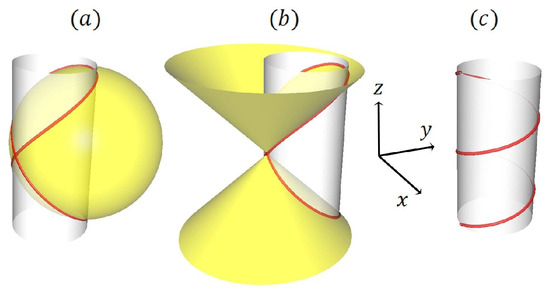
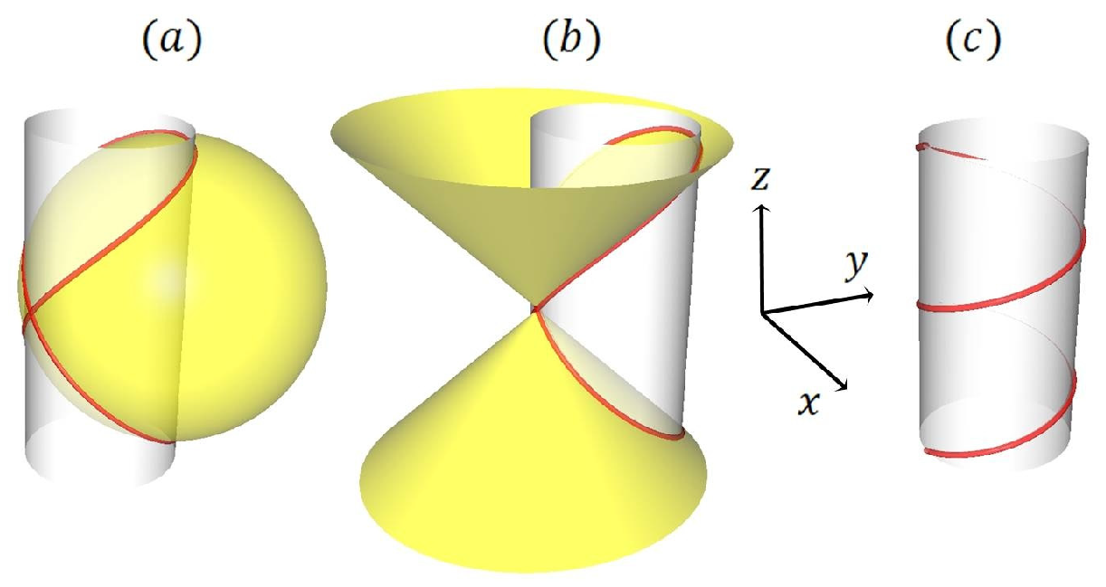
Inspired by an architectural problem, Viviani considered the cutting curve between a sphere of unit radius $r=1$ and a cylinder (radius $r/2$) passing through the center of the sphere (Figure 8a). The line of intersection is also known as the ‘Viviani window’, because the construction cuts a window into a spherical dome. This architecture-related discovery may be old, dating back to a disciple and biographer of Galileo, but the underlying multifaceted geometry remains a useful and up-to-date tool in non-Euclidean settings too. When interpreted as a spacetime curve, this geometric object literally opens up a visual window upon spinorial properties, using various representations in Minkowski spacetime. The $x,y$-plane represents spatial variables, while the vertical $ct$-axis represents time. This implies that the squared spacetime distance between two events is given by $\mathsf{\Delta }{s}^2=c^2{\Delta t}^2-({∆x}^2+{∆y}^2)$. It remains invariant for all observers, unaffected by their motion. With this interpretation, it becomes evident that the Viviani curve also ‘lives’ on the lower and upper light cones, defined by $\mathsf{\Delta }{s}^2=0$, as illustrated by the intersection of a rectangular double cone and a cylindrical tube (Figure 8b).

Figure 8. (a) The red Viviani curve formed by the intersection of a sphere and a cylinder. (b) The curve as the intersection of a cylinder and a rectangular double cone. (c) Two rotations of the red lightlike helical worldline of the charge center on the cylinder surface (see the text for details).

In the spacetime interpretation, the cylindrical tube in Viviani’s original construction is considered to carry the worldline of the internal rotation of the charge center, which rotates at twice the Compton frequency. It describes a lightlike helix along the cylindrical surface (see Figure 8c). The radius of the cylinder is half that of the sphere, and is equal to the ZBW amplitude ${\mathrm{ƛ}}_{\mathrm{C}}/2$. Since the helix is unbounded in the vertical direction, the Viviani curve provides a compact representation of the periodic temporal progression of the worldline. Thus, the images condense periodic phase-dependent processes into closed geometric forms. These reveal topological properties relevant to representations of spin-related phenomena, which will be discussed next.

5.3. Topologically Equivalent Representations: From Viviani’s Window to the Möbius Band and Toroidal Embeddings

The Möbius band is the best-known geometric model for visualizing the topological properties inherent in complex-valued spin vectors (spinors). Long before electron spin was discovered, Möbius conceived this paper strip model to illustrate a one-sided surface. It consists of a rectangular strip of paper long enough to allow the ends to be glued together after twisting them by 180°. It is a non-orientable, two-dimensionalmanifold that can be embedded in ordinary, three-dimensional space. A $4\pi$-rotation along the band is required to return to the starting point. The same applies to the state of an electron in Hilbert space, which must be rotated by $4\pi$ before the initial value of the complex wave function is restored.

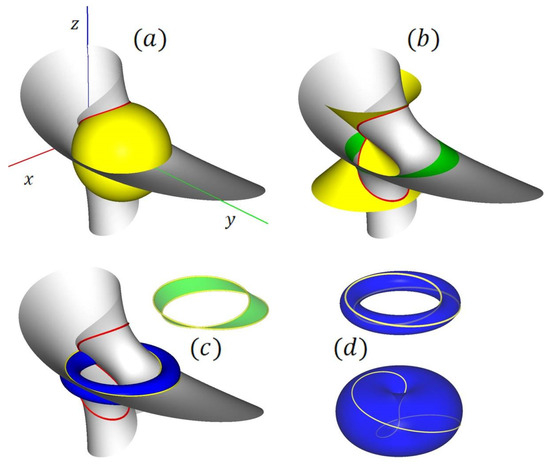
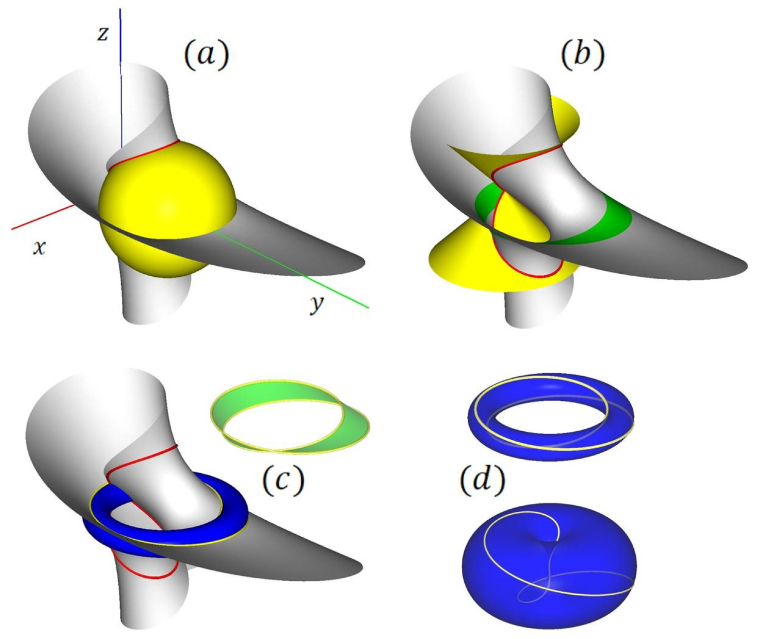
To demonstrate the relationship between the Möbius band and the Viviani curve, we first consider the Möbius surface. This is an unfamiliar-looking ruled surface (Figure 9a) that can be created as a surface of revolution by rotating a line along a circular guiding line.

Figure 9. A survey of various representations of the green Möbius band and its yellow edges derived from the red Viviani curve on the gray Möbius surface. In (a) the Viviani curve is generated by the intersection of the Möbius surface and the yellow unit sphere. Image (b) shows the Möbius surface and the light cone intersection. The Möbius band is also shown. Image (c) highlights the edges of the band. The intersection of the blue open ‘donut’ torus with the Möbius surface also traces out the edge lines. Image (d) shows the edge lines on the open torus and on the horn torus. See the text for the underlying parametric representations.

Imagine a propeller (radius $v$) rotating along a circle of unit radius, with the propeller axis always pointing tangentially to the guiding circle. Set the angular velocity of the propeller rotations to half the angular velocity along the circle. The center of the guiding circle is positioned at $(\mathrm{0,1},0)$. This results in the following Cartesian parametrization of the surface $(0\le u\le 2\pi , -2\le v\le 2$):

$$x\left(u,v\right)=\left(1+v\mathit{cos}u\right)\mathit{sin}2u$$

$$y\left(u,v\right)=\left(1+v\mathit{cos}u\right)\mathit{cos}2u+1$$

$$z\left(u,v\right)=v\mathit{sin}u$$

(12)

The Möbius band is part of this surface [20]. It is formed by rotating a line of length $v$ with $-a\le v\le a$ and $a<1.$ Figure 9a shows the Viviani curve as the intersection of a Möbius surface and a unit sphere, while Figure 9b uses the intersection with light cones instead. A Möbius band ($a=0.2)$ is also added. Figure 9c illustrates the band and its edges separately, including the intersection between the Möbius surface and an open torus. The band’s edges are parametrized by ($0\le u\le 2\pi , a=0.2)$:

$$x\left(u\right)=\left(1+a\mathit{cos}u\right)\mathit{sin}2u,$$

$$y\left(u\right)=\left(1+a\mathit{cos}u\right)\mathit{cos}2u+1$$

$$z\left(u\right)=a\mathit{sin}u,$$

(13)

With unit radius for the center line and radius $a$ for the toroidal hose, and with the angular variable u and v both in the interval $\left[\mathrm{0,2}\pi \right]$, the open torus is defined as follows:

$$x\left(u,v\right)=\left(1+a\mathit{cos}u\right)\mathit{sin}v$$

$$y\left(u,v\right)=\left(1+a\mathit{cos}u\right)\mathit{cos}v+1$$

$$z\left(u,v\right)=a\mathit{sin}u$$

(14)

A horn torus $(a=1)$ provides an alternative representation. Figure 9d illustrates how spinorial characteristics, which require a $4\pi$-rotation to return to the original state, can be represented by the edge lines circulating different toroidal surfaces.

Shrinking the width of the Möbius band reveals that the Viviani curve can be transformed topologically onto a circle by elastically stretching the two branches along the Möbius surface. For a finite width, this process projects the curve onto antipodal points on the Möbius band, thereby preserving double coverage. Thus, the Möbius band and its toroidal embeddings are different, yet topologically equivalent, representations of spin-like properties. They are related to the Viviani curve via homeomorphism.

Finally, we highlight the distinction between the paper strip model and the Möbius band illustration in Figure 9, a detail that is often overlooked. Unlike the analytic representation on which the graphic is based, the paper strip is a developable surface [21,22]. However, this fact is not relevant to the current topological considerations.

6. Electron Spin and the Gyromagnetic Ratio in Two-Center Models: Implications of Double Covering

6.1. Connections of the Present Approach with Related Two-Center Electron Models

Scattering experiments reveal that electrons have no internal structure. Even at the highest available collider energies, they appear as point-like objects. However, attempts to describe ZBW and spin in less abstract terms using geometric representations suggest the existence of local or internal degrees of freedom that differ from those describing the particle as a whole. Intuitively, these can be attributed to the near field surrounding the electron, emerging from interactions with the quantum vacuum.

Such an interpretation of electromagnetic radiation confined to the near field is non-radiating, as it does not contribute to radiation in the far field. Non-radiating sources are important in photonic technology [23]. An elementary explanation is given in [24]. A freely propagating photon field has no rest mass because it propagates at the speed of light. However, when the field is confined, it acquires mass because accelerating the containment, which is considered massless, requires force [25]. In a way, mass behaves like canned energy. Rest mass refers to the center of mass of a closed system considered completely at rest. However, this state is an idealization, as it does not account for the internal degrees of freedom that oscillate at the speed of light, giving rise to ZBW. According to this view, the mass and spin of an electron both result from effects residing in the near field.

The current line of modeling ZBW quasi-mechanically by an antiparallelogram linkage and reducing it to a two-center description is novel. This approach paves the way for more appropriate $(1+2)$-dimensional spacetime models of ZBW and electron spin. It aligns with a spectrum of similar efforts that have emerged from the desire to improve the understanding of the abstract, nonclassical properties of spinors by using more accessible mechanical and geometric models. Here, we limit the references to articles that are related to the present models.

Hestenes provides the most elaborate theoretical analysis based on the language of geometric algebra [26]. He interprets ZBW realistically as a local circulatory motion of an electron at the speed of light, which he considers to be the origin of the electron spin and magnetic moment [27]. The topological aspects of electron models based on the confinement of lightlike entities are described in [28]. A particular focus on toroidal models is given in [29].

In the context of quasi-classical mechanical two-center electron descriptions, the model elaborated by Rivas is also relevant [30,31]. It provides a detailed description of the existence of two centers, CM and CC, as well as the rotation of the CC at the speed of light. Despite being based on a different theoretical framework, the model largely aligns with the current description.

However, unlike the Rivas model, the current description uses ad hoc assumptions about the system that reduce the motion of internal mechanical degrees of freedom to a two-center description. When translated into a spacetime framework, the resulting dynamics corresponds to the CM and CC trajectories of these two-center electron models. To verify consistency, we calculate electron spin and magnetic moment of the extended $(1+2)$-dimensional spacetime model, starting from the Viviani curve.

6.2. Planar Rotations of the Charge Center and the Z-Component of Spin and Magnetic Moment

In the compact representation of Figure 7, the Viviani curve is composed of two frequencies. The first, ${\omega }_0$, describes timelike cycles and is represented by vertical oscillations at unit amplitude. The planar projection of the spacelike $x,y$ components results in a double-covered circle underlying ZBW at half amplitude and double frequency. To calculate the resulting angular momentum from this planar rotation, the lightlike nature of the CC rotation must be taken into account. Due to confinement, this photon-like entity, which has an energy of $E=\mathbf{\hslash }{\mathsf{\omega }}_0$, obtains a mass according to $E=m{c}^2$ [32]. The resulting angular momentum of the CC propagating at the speed of light along the planar circle is equivalent to the photon momentum $p_{ph}=mc=\mathbf{\hslash }{\mathsf{\omega }}_0/\mathrm{c}$. For simplicity, only the magnitudes are considered. If necessary, the vector notation in bold is used. The intrinsic rotation of the CC along a circle with radius $r={\mathrm{ƛ}}_{\mathrm{C}}/2=\mathbf{\hslash }/2mc=\mathrm{c}/2{\mathsf{\omega }}_0$ yields the z-component of the angular momentum $S_z=r·p=\hslash /2$ which is the model’s analog of electron spin.

The $z$-component of the magnetic dipole moment ${\mu }_Z$ produced by the elementary charge $e$ in circular motion is equal to the product of the current $I$ and the area $A$ of the current loop. Note that, due to the negative sign of the charge, the vectors of magnetic moment and orbital rotation point in opposite directions. The length of one ZBW period at twice the Compton frequency ${\omega }_0$ is $T_z=\pi /{\omega }_0$. With the current $I={e/T}_z=e{\omega }_0/\pi$, and the area $A=\pi c^2/4{\omega }_0^2$ one obtains ${\mu }_Z=e{c}^2/4{\omega }_0=e\hslash /4m$.

This value for an orbiting charge also corresponds to the classical magnetic dipole moment of a rotating charged sphere, which is half the magnitude of the Bohr magneton ${\mu }_B=e\hslash /2m$ (cf. [33]). However, the experimental value for an electron is approximately twice as large. This discrepancy from the classical expectation is expressed by the gyromagnetic ratio of $g=2$, yielding ${\mu }_z={\displaystyle \frac{1}{2}}g{\mu }_B$.

The above calculation of ${\mu }_Z$ is based on a single current loop and does not take into account double coverage, which underlies the planar projection of the Viviani curve onto the $x,y$-plane. This feature is shown schematically in Figure 7 and in the torus models in Figure 9. Provided that the radius of the toroidal hose is extremely small, two connected loops of nearly the same radius are formed. In the present calculations, we neglect this small yet finite difference. Two identical current loops produces twice the magnetic moment, resulting in the gyromagnetic ratio of $g=2$. This is the value predicted by the Dirac equation. It applies to a ‘bare’ or ‘undressed’ electron, which does not experience additional small corrections, which are described by electron–photon interaction loops in quantum electrodynamics (QED). These corrections are not discussed further in this paper because they require additional model assumptions.

From a purely classical perspective, the gyromagnetic ratio of $g=2$ was an enigmatic empirical factor in the early days of quantum physics. However, it can be naturally explained by the topological properties of electron spin as an internal property, which includes interactions with the quantum vacuum. Coupling to the surrounding environment requires a $4\pi$-rotation of the whole structure including near field interactions in order to return to the initial state. Due to this double coverage, the electron is twice as effective as a single loop or a rotating charged sphere at generating a magnetic moment. These near-field effects resemble the Dirac string model mentioned in the introduction, with twisted strings representing interactions respectively field lines confined to the near-field. They keep track of the rotation history in spacetime.

6.3. Semiclassical Picture of Electron Spin and Precession in a Magnetic Field

Thus far, the model’s planar rotation of CC, confined to the $x,y$ plane, accounts for only one component of spin and magnetic moment. However, obtaining the total spin requires including all three components. As in classical angular momentum algebra, the magnitude of the total spin $\mathit{S}$ is given by $\left|\mathit{S}\right|=\sqrt{{\mathit{S}}_{\mathit{x}}^2+{\mathit{S}}_{\mathit{y}}^2+{\mathit{S}}_{\mathit{z}}^2}=\sqrt{3}/2 \mathbf{\hslash }$. With the intrinsic electron spin $s=\mathrm{\hslash }/2$, this is identical to the quantum mechanical result $\left|\mathit{S}\right|=\sqrt{\mathrm{s}\left(\mathrm{s}+1\right)}\mathrm{\hslash }$. The electron’s total magnetic moment, with $g=2$ included, is given by

$$\mathit{\mu }=-{\displaystyle \frac{e}{m}}\mathit{S}.$$

(15)

Depending on the direction of the planar rotation of CC $\mathit{\mu }$ is either parallel or antiparallel to the total spin. An additional magnetic field $B$ exerts a torque $\mathit{\tau }=\mathit{\mu }\times \mathit{B}$ on $\mathit{S}$, which tends to align the magnetic moment with the magnetic field. As $\left|\mathit{S}\right|$ is conserved, this results in precession around the axis given by the direction of the magnetic field.

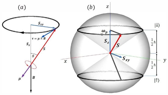
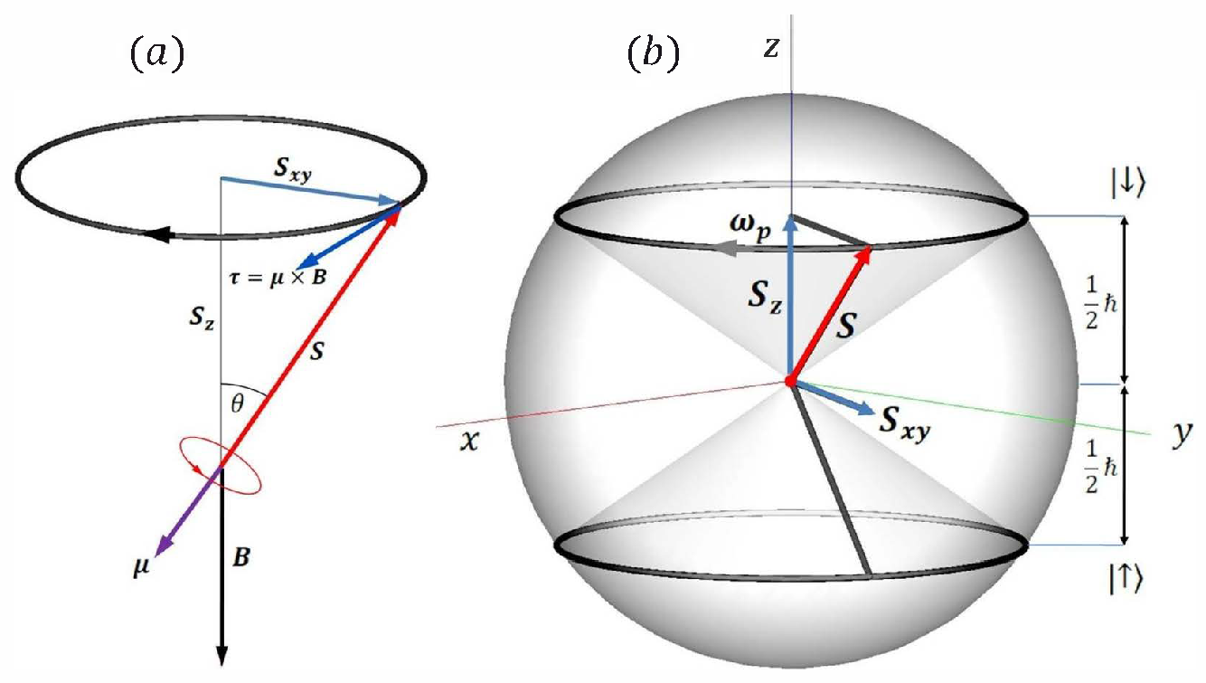
Figure 10a shows the vector model, with $B$ pointing in negative direction. This situation is analogous to a spinning top under the influence of gravity. Figure 10b illustrates the resulting spin precession. Note that, while related, this semiclassical picture is not fully equivalent to the Bloch sphere visualization of electron spin. Note the difference in meaning between the spin components in both pictures. The classical description refers to the vector components of spin as a three-component vector in physical space. In contrast, the quantum description refers to the spin-up and spin-down components of the spin wave function in spinor space. This essential distinction must be kept in mind for the following discussions.

Figure 10. (a) Vector model of spin precession with $\mathit{B}$ pointing in negative $z$-direction. Precession is driven by the torque $\mathit{\tau }=\mathit{\mu }\times \mathit{B}$. In the case shown, the magnetic moment $\mathit{\mu }$ and the total spin $\mathit{S}$ are antiparallel. This corresponds to the CC rotating counterclockwise. Diagram (b) presents a semiclassical picture of spin precession. $|\uparrow ⟩$ and $|\downarrow ⟩$ denote spin-up and spin-down states. In the low-energy spin-up state $|\uparrow ⟩$, ${\mu }_z$ points into the direction of the magnetic field. In the spin-down state it points in opposite direction. In both cases the direction of precession is the same. See the text for details and for obtaining the precession frequency ${\omega }_P$.

It is important to address the limitations of a classical model, which refers to an individual particle and relies on completely determined phase factors. This facilitates the simultaneous determination of the total spin and each spin component. In contrast, in the quantum case, it is only possible to measure the spin magnitude and one component simultaneously.

As the position of $\mathit{S}$ during precession is unknown due to phase uncertainty, only the $z$-component of the total spin is known. It remains constant during precession. There are two spin components, corresponding to the spin-up and spin-down states, which have different energies. In the low-energy spin-up state, denoted by $|\uparrow ⟩$, $\mathit{\mu }$ tends to align with the magnetic field. In the high-energy spin-down state $|\downarrow ⟩$, it tends to anti-align. The two orientations of $\mathit{\mu }$ are defined by clockwise and counterclockwise planar rotations of the CC. Unlike common textbook images, the precession of the spin-up state in Figure 10b occurs below the $xy$-plane because B points in negative z-direction. This direction is chosen to maintain the analogy with a spinning top under gravity.

The precession frequency ${\omega }_P$ can be calculated in analogy to the spinning top. The change in angular momentum $\mathit{S}$ due to a torque $\mathit{\tau }$ is given by $\mathit{\tau }=d\mathit{S}/dt={\mathit{\omega }}_{\mathit{P}}\times \mathit{S}$. The magnitude is the scalar product $dS/dt={\omega }_{P}S\sin \theta ={\omega }_P{S}_{xy}$ with $S\sin \theta =S_{xy}$ (see Figure 10a). This gives ${\omega }_P=\tau /S\sin \theta$. Inserting the torque $\tau ={\displaystyle \frac{e}{m}}SB\sin \theta$ exerted by the field on the electron’s magnetic dipole moment yields the precession frequency.

$${\omega }_P={\displaystyle \frac{e}{m}}B={\displaystyle \frac{2}{\hslash }}{\mu }_{B}B=\mu B.$$

(16)

The precession frequency is proportional to the energy gap between the low- and high-energy states, given by $∆E=\mathbf{\hslash }{\omega }_P=(\hslash e/m)B$. The energy difference defines the resonance frequency, which is at the core of many important magnetic resonance technologies. These range from electron spin resonance (EPR) and nuclear magnetic resonance (NMR) to magnetic resonance imaging (MRI). MRI is an important, noninvasive technique used in medical diagnostics. The foregoing derivation helps to understand these technologies from a quasi-classical mechanical perspective with a few quantum mechanical caveats added.

7. Coupled Oscillators, Cogwheel Systems, and Phase Models: The Role of Classical Ontology in the Interpretation of Quantum Phenomena

This concluding retrospective evaluates the strengths and weaknesses of transforming a fully concrete mechanical system into a more abstract analog of ZBW and spin. It discusses the overarching dynamical and symmetry principles that underpin the effectiveness of this approach. Finally, since the rotating gear wheels stand for phase variables, the role of cyclic variables in bridging classical and quantum descriptions deserves closer consideration. As this topic touches upon deep and controversial ontological questions, it is still under development and far from finalized.

7.1. The Potential and the Limits of Concrete Spin and ZBW Models

The model’s primary merit lies in its heuristic function and its potential to demystify the strange, classically indescribable, two-valued manifestation of electron spin, which is useful for educational purposes. It uses a reverse engineering method based on intermeshing classical gear wheels or mechanical linkages. Starting from a fully concrete and tangible mechanical system, the semiclassical interpretation requires abstraction and a leap to a description in terms of relativistic spacetime. Its $\left(1+2\right)$-dimensional spacetime extension offers a quasi-classical interpretation of ZBW and spin, assuming the rotation of a charged, photon-like entity confined within a topology affording double coverage. However, any interpretation of the model must respect its hybrid nature, which is based on incorporating correspondences with special relativity and quantum mechanics. This is in accordance with the Dirac caveat that the system provides a more abstract correspondence than a close analogy.

On a concrete level, it illustrates the connection to angular momentum of an internal degree of freedom in a two-center description. On an abstract level, it reveals spin as a rotation in spacetime that transcends our common-sense understanding of ordinary rotations. Thus, it conveys as far as possible a tangible experience of spin, although it is an abstract, inherently relativistic quantum property. Furthermore, it draws attention to another important fact. Contrary to the common view that relativity only applies to objects moving at relativistic velocities, it highlights the relativistic nature of spin, which is equally dominant in the non-relativistic domain. This includes the description of spinning particles at rest or moving at small, non-relativistic velocities.

A weakness of the model is that the two-center description is purely kinematic and ad hoc. It presupposes the existence of an elementary charge. It does not explain the physical mechanism behind the decomposition into CM and CC, nor does it explain how a lightlike object is confined to a structure on the scale of a Compton wavelength. In a way, these limitations are the price we pay for such a largely concrete description. However, to a certain degree, the model’s intuitive, visual, and tangible nature outweighs this blind spot.

Another limitation of the present analysis concerns approximations of the anomalous magnetic moment. They quantify the discrepancy between the bare gyromagnetic ratio of $g=2$ and the results of precision measurements or theoretic loop corrections based on QED. The deviation is defined as $a=(g-2)/2$. The largest first-order correction from a series expansion obtained by QED yields $a={\displaystyle \frac{\alpha }{2\pi }}$, where $\alpha \approx 1/137$ is the fine structure constant [34]. In principle, similar corrections could be incorporated into the current model based on a detailed numerical analysis of the edge trajectories in the toroidal representations in Figure 9. Similarly, related toroidal representations approximate the first term of standard QED loop corrections (see references [26,29]). However, since additional model assumptions beyond the current framework are necessary, this issue will be addressed in future work.

Whether one appreciates the potential of semiclassical models as a useful complement to established theories is a matter of personal epistemology. From a formal perspective, classical models are bound to fail, and semiclassical approaches cannot fully compete with established explanations and replace the extremely successful approaches of quantum mechanics (QM) or quantum electrodynamics (QED). However, even within the established theories, the interpretation of ZBW, and its relationship with spin remains controversial to this day. Standard QM describes ZBW as the interference between positive and negative energy contributions in the Dirac equation [35]. In the QED framework, it results from the interaction with the vacuum. Some theorists even doubt the physical reality of ZBW, considering it a mathematical artifact arising from attempts to impose a single-particle description [36].

At present, direct observation of ZBW with electrons appears to be unfeasible due to the exceedingly high frequency $(~{10}^{21} \mathrm{H}\mathrm{z})$ and the small amplitude ${(~10}^{-13} \mathrm{m})$, though experimental indications have been reported based on channeling experiments [37]. Successful quantum simulations of ZBW in different physical platforms have been carried out, for instance using trapped ions [38], Bose–Einstein condensates [39], and photonic systems [40]. ZBW and its effects on electrons in condensed matter systems are reported in [41,42], based on the analogy between the band structure of narrow-band semiconductors and the Dirac equation. Simulations of ZBW in classical systems can be found in references [43,44]. Due to the wide range and complexity of these analogies, the potential of the current quasi-mechanical approach to provide an introductory experience cannot be overestimated.

7.2. Overarching Dynamical and Symmetry Principles Underpinning the Effectiveness of the Models

There are more general principles hidden beneath the seemingly coincidental relationship between the mechanistic two-center kinematics and spin models, which are of particular interest. The model’s ability to successfully incorporate ZBW, spin, and magnetic moment depends on its hybrid nature, which encompasses universal properties of nonlinear phase dynamics and general symmetries. It builds upon synchronization, a multifaceted and cross-cutting dynamical phenomenon in driven or coupled oscillators that establishes coherence in a wide spectrum of systems, ranging from basic classical science and technology to quantum technologies. The laser is a key paradigm of coherence and self-organization in quantum systems [45]. The underlying principles also apply to a wide spectrum of other fields and paved the way for the trans-disciplinary field of synergetics. In everyday physics, for example, there are intriguingly simple classical models of synchronization that demonstrate the potential of self-organization and coherence in various stages of biological information dynamics [46,47].

Another fortuitous fact that was not anticipated when developing mechanical sync analogues is the parallelism between phase modulation and the dynamics of elliptical gears or antiparallelogram linkages, used to produce gear-driven linear propagation. Nonlinear phase dynamics provides a self-regulating mechanism between energy and momentum that aligns with relativistic dispersion in a propagating system. A third relevant feature is the reduction to a two-center description, which exhibits spin-like behavior. The latter is represented by the Viviani curve and its various topologically equivalent embeddings.

Beyond that, the dynamics of states along the Viviani curve reveals fundamental symmetries that are essential to the spin analogy. This fact, which was not obvious in the early stages of developing the phase model, offers a broader, more abstract perspective on the model’s effectiveness. The points of intersection between the Viviani curve and the Gerono lemniscate reveal these symmetries. We study these points for a Viviani curve with a vertex at $(\mathrm{0,1},0)$ that intersects a Gerono lemniscate oscillating along the $y$-axis according to $y\left(t\right)=(1+\sin \left(2{\omega }_{0}t\right))/2$.

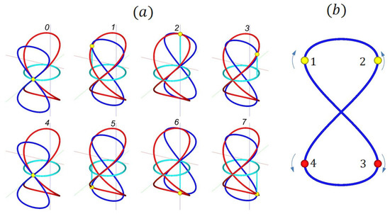
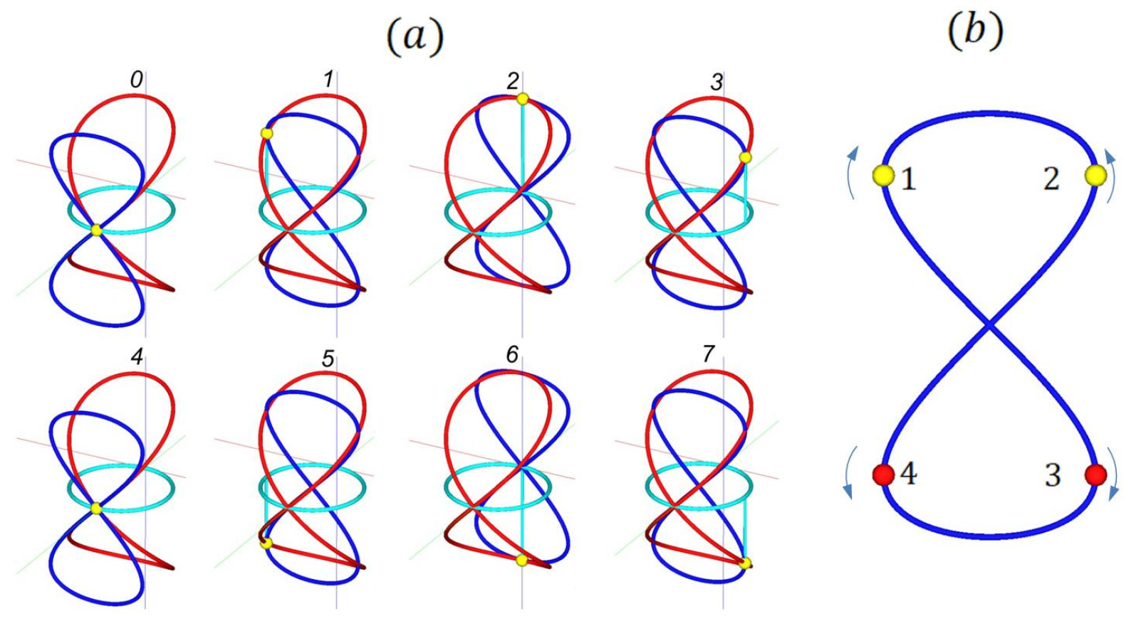
Figure 11a shows the position of a specific state as it propagates along the Viviani curve. It is marked by a small sphere and results from the clockwise double-covered planar rotation that yields ZBW. A series of snapshots illustrates all intersections with the oscillating Gerono lemniscate, separated by one-eighth of the ZBW period $T_{ZBW}=\pi /{\omega }_0$. There are four crossing points except at the inflection points of the oscillation. Two are at $y=0$ and one is at $y=1$. The state denoted by 1 in Figure 11b corresponds to snapshot 1 in Figure 11a. It depicts an electron state in clockwise rotation. State 2 is the mirror image of state 1, with the mirror located in the $yz$-plane at$x=0$. This reflection reverses the handedness of the rotation vector, thereby flipping the particle’s helicity (see [48] for a definition). Yellow indicates electron states.

Figure 11. (a) Successive snapshots of the dynamics along the red Viviani curve in spacetime. One oscillation cycle at ${\omega }_0$ along the vertical timelike axis is shown. It is connected to the clockwise rotation (light blue) in the $xy$-plane at the ZBW frequency ${2\omega }_0$ (red $x$-axis, green $y$-axis). The blue Gerono lemniscate oscillates at ${2\omega }_0$ along the $y$-axis. A yellow sphere represents the propagating state along the Viviani curve as well as one point of intersection that circulates along the Gerono lemniscate. A vertical projection connects this state to the planar circle. The numbers are successive fractions of 1/8 of the ZBW period. Diagram (b) shows the four crossing points, interpreted as particle (yellow) and antiparticle (blue) states. The arrows indicate their different handedness. See the text for details of the underlying symmetries.

The red spheres below the $xy$-plane represent antiparticle states, i.e., positrons. These states can be obtained from the electron states in two equivalent ways: by rotating 180° around the $y$-axis, or by performing two orthogonal reflections. Reflection by the vertical plane flips the particle’s helicity, reflection by the horizontal plane at $z=0$ involves charge conjugation, converting an electron into a positron.

A further symmetry refers to the direction of time. Antiparticle state 3 can be transformed back into particle state 1 by inverting time. This aligns with the Feynman–Stückelberg interpretation, that antiparticles correspond to particles traveling backward in time. The existence of antiparticles is formally encoded in the energy spectrum, as given by the relativistic energy dispersion formula $E=\pm \sqrt{E_0^2+{\left(pc\right)}^2}$ [49]. This includes an energy gap $∆E=2E_0$ that separates particles from antiparticles, and the square root allows for positive and negative energies outside the gap. For negative energy, the time-dependent phase term in the wave function is $-Et$. This is equivalent to positive energy and a negative time parameter.

While this may sound unusual for a classical particle, synchronization exhibits equivalent symmetries expressed by negative frequencies. These appear much less mysterious than negative energies. Complete phase locking occurs within a frequency gap of width $∆\omega =2{\omega }_0$. The free-running state outside the locking region is characterized by a positive beat frequency ${\omega }_B$, when detuned positively, and by $-{\omega }_B$, when detuned negatively (see the symmetry in Figures 2 and 3 in [5]). Negative frequencies simply reverse the rotation of the phase pointer. Switching to the free-running phase at the lower and upper critical frequencies involves a second-order phase transition, characterized by square-root dependence of the beat frequency ${\omega }_B$.

According to the classical-quantum correspondences of the model, the locking bandwidth corresponds to the energy gap $∆E=2E_0$, which is required to create a particle-antiparticle pair. In the free-running state of the sync model, ${\pm \omega }_B$ corresponds to particle and antiparticle states, described by positive and negative energy. The square-root dependence of $\pm E$ in beyond the critical points conforms to a second-order phase transition.

Thus, a connection is established between the principles of sync-based self-organization in classical oscillators and a phenomenological model of particle creation and their relativistic dynamics. This opens up a coherent perspective on the overarching role of self-structuring processes and the emergence of new properties across all scales, from the very large to the very small.

The underlying symmetries that transform the four particle states in Figure 11b pertain to a model with two spatial and one temporal dimension. These operations provide a simplified representation of the symmetries described by the CPT theorem in particle physics, which establishes connections between charge conjugation, parity transformations, and time inversion.

7.3. Aspects of Ontological Parallels Between Classical and Quantum Phases

The phases of oscillators and their parameter dependent transition from locked to modulated phases are central to the present semiclassical analogies. These are extended by a structured sequence of stepwise model refinements to demystify quantum properties, such as spin and ZBW. The starting point is illustrated in Figure 1. It shows how nonlinear phase dynamics can be mapped onto the overdamped motion of a ‘phase particle’ along a tilted washboard. This particle ontology also applies when the local phase dynamics is extended to propagating elliptical gears and equivalent antiparallelogram linkages. Propagation in proper time is described by the proper velocity $v_{prop}=p/m=c\beta \gamma$. An observer at rest measures the coordinate velocity as $v_{coord}=v_{prop}/\gamma =\beta c$, which is identical to the group velocity in quantum mechanics $v_{gr}=dE/dp=c^{2}p/E$.

The wave concept of group velocity highlights the clash between the classical particle ontology and the quantum interpretation. In the classical framework, the state of an individual ‘phase particle’ in phase space is described by a well-defined momentum and position. Superposition of states is impossible. This is the reason why the present ZBW explanation in a two-centermodel differs from the standard QM interpretation, which is based on interference between positive and negative frequency modes in localized wave packets. In contrast, quantum representations depend on the superposition of continuous distributions of momentum states. The product of the standard deviations of momentum and position is limited by the uncertainty relation $∆x∆p\ge \hslash /2$. Individual phases are not observable; only phase differences can be measured.

Various approaches have been proposed to bridge the gap between the disparate ontologies of phase variables in classical and quantum systems. In the present model, the rotating gears imply an analogy to the phase in driven open quantum systems, where openness is attributed to interactions with the quantum vacuum. This model most closely resembles the relationship between a quantum harmonic oscillator and a classical particle moving in a circle. As analyzed by ‘t Hooft [50,51], the temporal evolution of a quantum harmonic oscillator is identical to that of a classical rotator. Consequently, the quantum phase can be considered a hidden ontological variable. While the individual phases of the quantum states contributing to the ensemble are veiled by quantum uncertainty, the emerging phase of the ensemble has a real status, just like the classical phase.

We propose that the present phase model is another example of a dual relationship between classical and quantum phase. It establishes coherence among coupled or driven classical oscillators and coherent quantum states, which most closely conform to a classical description. They minimize the uncertainty between complementary variables, such as momentum and position, or amplitude and phase. Their temporal evolution remains maximally localized, and their expectation values evolve in exactly the same way as position and momentum in a classical oscillator.

Thus, the assumption of a dual relationship between classical and quantum coherence appears self-evident. However, a connection with coherent quantum rotator or oscillator states is not straightforward and requires closer scrutiny. There are subtle differences as the eigenstates of a free rotator have an undefined phase. Specific superpositions of angular momentum states are required to form coherent states on a circle that mimic well defined position and momentum of a classical particle orbiting on a circle (see [52,53] for theoretical descriptions). This short overview shows that coherent oscillator or rotator states can, to some degree, reconcile the differences in the ontologies of phase variables in classical and quantum systems, provided that the specific character of these states is respected.

8. Conclusions: A Pledge for the Plurality of Models on the Road to Abstraction

The rapid development of modern quantum technologies challenges us to convey the counterintuitive nature of quantum phenomena to a much wider audience. At its core, the strangeness and abstractness of the quantum world, and of all its applications, which transcend many of our classical intuitions, are deeply rooted in relativity, both special and general. The present approach is based on semiclassical dynamic models that incorporate geometric and topological representations as well as fundamental symmetry principles. It transfers principles of synchronization-based self-organization and emergence to the realm of particle physics, thus elucidating the universal nature of these concepts and their application to various fields in science and rapidly evolving quantum technologies.

In the endeavor to make sense of intricate and theoretically demanding quantum phenomena, it is indispensable to use heuristic approaches, as well as model-based explorations and explanations, in order to overcome the constraints of our classical intuition. Since any interpretation ultimately recurs to some kind of concrete experience or representation, successful models should clarify and embody the relevant functional and structural principles underlying the domain of interest. These core ideas can be communicated in various ways, each with a different impact on promoting a deeper understanding. For example, they can be communicated verbally, visually, or experience based through interactive experiments, simulations and analog constructs, including adequate theoretical embeddings.

To promote a more comprehensive understanding, it is essential to consider the problem from multiple perspectives and explore different theoretical approaches, models, and representations. In the present study, the stepwise development of the model’s building blocks, based on analogies, concrete implementations and geometric representations, reflects the variety of the conceptual levels involved. The models face conceptual and interpretational challenges that are closely related to those of full-fledged formal theories, albeit at a more concrete and intuitive level.

In this context, the following quote by Bohr, which goes back to Schiller’s ‘Proverbs of Confucius’, aptly captures this productive tension between the plurality of models and the abstract principles they stand for [54]:

“Only fullness leads to clarity,

And truth lies in the abyss.”

This fullness or wholeness involves deploying various models and methods to better understand the multifaceted nature of an underlying abstract reality. Wholeness is based on complementary ways of thinking and modeling that intertwine concrete, experience-based, informal approaches with abstract, theory-driven, formal methods (see related examples in [55]). In order to come to terms with the ‘abyss’ of an abstract truth that is difficult to grasp in concrete terms, one must be willing to interact productively with conflicting views and theories and tolerate ambiguity.

References

- Pauli, W. Remarks on the History of the Exclusion Principle. Science 1946, 103, 213–215. [Google Scholar] [CrossRef] [Scilit] [PubMed]
- Dirac, P.A.M. The Principles of Quantum Mechanics; International Series of Monographs on Physics, No. 27; Oxford University Press: Oxford, UK, 1981. [Google Scholar]
- Penrose, R.; Rindler, W. Spinors and Space-Time; Cambridge University Press: Cambridge, UK, 1984; Volume 1, p. 43. [Google Scholar]
- Euler, M. The Mechanics of Synchronization: From Phase Modulation to Elliptical Gears with Quasi-Relativistic Properties. Appl. Mech. 2025, 6, 37. [Google Scholar] [CrossRef] [Scilit]
- Euler, M. Universal synchronization: Acoustic experiments, the phase oscillator model and mechanical analogues. Eur. J. Phys. 2024, 45, 023003. [Google Scholar] [CrossRef] [Scilit]
- Schrödinger, E. Über die kräftefreie Bewegung in der relativistischen Quantenmechanik. Sitzungberichte Preuss. Akad. Wiss. Phys.-Math. Kl. 1930, 24, 418–428. [Google Scholar]
- Adler, R. A study of locking phenomena in oscillators. Proc. IRE 1946, 34, 351–357, Reprint in Proc. IEEE 1973, 61, 1380–1385. [Google Scholar] [CrossRef] [Scilit]
- Figliolini, G.; Lanni, C.; Ceccarelli, M. On the kinematic synthesis of non-circular gears. Int. J. Gearing Transm. 2000, 3, 90–98. [Google Scholar]
- Apostol, T.M.; Mnatsakanian, M.A. Unwrapping curves from cylinders and cones. Am. Math. Mon. 2007, 114, 388–416. [Google Scholar] [CrossRef] [Scilit]
- Jameson, G.J.O. Inequalities for the perimeter of an ellipse. Math. Gaz. 2014, 98, 227–234. [Google Scholar] [CrossRef] [Scilit]
- Fraundorf, P. A one-map two-clock approach to teaching relativity in introductory physics. arXiv 1996, arXiv:physics/9611011. [Google Scholar]
- Rindler, W. Relativity: Special, General, and Cosmological; OUP Oxford: Oxford, UK, 2006. [Google Scholar]
- de Broglie, L. Ondes et quanta. Comptes Rendus Acad. Sci. 1923, 177, 507–510. [Google Scholar]
- de Broglie, L. Recherches sur la théorie des quanta. Ann. Phys. 1925, 3, 22–128. [Google Scholar] [CrossRef] [Scilit]
- Messerschmitt, D.G. Relativistic timekeeping, motion, and gravity in distributed systems. Proc. IEEE 2017, 105, 1511–1573. [Google Scholar] [CrossRef] [Scilit]
- Barut, A.O.; Bracken, A.J. Zitterbewegung and the internal geometry of the electron. Phys. Rev. D 1981, 23, 2454. [Google Scholar]
- Langer, J.C.; Singer, D.A. Reflections on the lemniscate of Bernoulli: The forty-eight faces of a mathematical gem. Milan J. Math. 2010, 78, 643–682. [Google Scholar] [CrossRef] [Scilit]
- Abbena, E.; Salamon, S.; Gray, A. Modern Differential Geometry of Curves and Surfaces with Mathematica; Chapman and Hall/CRC: Boca Raton, FL, USA, 2017. [Google Scholar]
- Viviani Curve. Available online: https://mathcurve.com/courbes3d.gb/viviani/viviani.shtml (accessed on 1 September 2025).
- Maschke, H. Note on the unilateral surface of Moebius. Trans. Am. Math. Soc. 1900, 1, 39. [Google Scholar] [CrossRef] [Scilit]
- Wunderlich, W. Über ein abwickelbares Möbiusband. Monatshefte Für Math. 1962, 66, 276–289. [Google Scholar]
- Todres, R.E. Translation of W. Wunderlich’s “On a developable Möbius band”. J. Elast. 2015, 119, 23–34. [Google Scholar]
- Yang, Y.; Bozhevolnyi, S.I. Nonradiating anapole states in nanophotonics: From fundamentals to applications. Nanotechnology 2019, 30, 204001. [Google Scholar] [CrossRef] [Scilit] [PubMed]
- Berry, M.; Foley, J.T.; Gbur, G.; Wolf, E. Nonpropagating string excitations. Am. J. Phys. 1998, 66, 121–123. [Google Scholar] [CrossRef] [Scilit]
- Van der Mark, M.B.; ‘t Hooft, G.W. Light is heavy. arXiv 2015, arXiv:1508.06478. [Google Scholar]
- Hestenes, D. Gyromagnetics of the electron clock. IEEE Access 2025, 13, 53772–53803. [Google Scholar]
- Hestenes, D. The zitterbewegung interpretation of quantum mechanics. Found. Phys. 1990, 20, 1213–1232. [Google Scholar] [CrossRef] [Scilit]
- Williamson, J.G.; Van der Mark, M.B. Is the electron a photon with toroidal topology. Ann. Fond. Louis Broglie 1997, 22, 133. [Google Scholar]
- Consa, O. Helical solenoid model of the electron. Prog. Phys. 2018, 14, 80–89. [Google Scholar]
- Rivas, M. Kinematical Theory of Spinning Particles: Classical and Quantum Mechanical Formalism of Elementary Particles; Springer: Dordrecht, The Netherlands, 2002. [Google Scholar]
- Rivas, M. The center of mass and center of charge of the electron. J. Phys. Conf. Ser. 2015, 615, 012017. [Google Scholar] [CrossRef] [Scilit]
- van der Mark, M.B. Quantum particle, light clock or heavy beat box? J. Phys.Conf. Ser. 2019, 1251, 012049. [Google Scholar] [CrossRef] [Scilit]
- Sebens, C.T. How electrons spin. Stud. Hist. Philos. Sci. Part B Stud. Hist. Philos. Mod. Phys. 2019, 68, 40–50. [Google Scholar] [CrossRef] [Scilit]
- Schwinger, J. On quantum-electrodynamics and the magnetic moment of the electron. Phys. Rev. 1948, 73, 416. [Google Scholar] [CrossRef] [Scilit]
- Thaller, B. The Dirac Equation; Springer Science & Business Media: Berlin/Heidelberg, Germany, 2013. [Google Scholar]
- Wang, Z.-Y.; Xiong, C.-D. Zitterbewegung in quantum field theory. Chin. Phys. B 2008, 17, 4170. [Google Scholar] [CrossRef] [Scilit]
- Catillon, P.; Cue, N.; Gaillard, M.J.; Genre, R.; Gouanère, M.; Kirsch, R.G.; Poizat, J.-C.; Remillieux, J.; Roussel, L.; Spighel, M.A. Search for the de Broglie particle internal clock by means of electron channeling. Found. Phys. 2008, 38, 659–664. [Google Scholar] [CrossRef] [Scilit]
- Gerritsma, R.; Kirchmair, G.; Zähringer, F.; Solano, E.; Blatt, R.; Roos, C.F. Quantum simulation of the Dirac equation. Nature 2010, 463, 68–71. [Google Scholar] [CrossRef] [Scilit] [PubMed]
- LeBlanc, L.J.; Beeler, M.C.; Jimenez-Garcia, K.; Perry, A.R.; Sugawa, S.; Williams, R.A.; Spielman, I.B. Direct observation of zitterbewegung in a Bose–Einstein condensate. New J. Phys. 2013, 15, 073011. [Google Scholar] [CrossRef] [Scilit]
- Lovett, S.; Walker, P.M.; Osipov, A.; Yulin, A.; Naik, P.U.; Whittaker, C.E.; Shelykh, I.A.; Skolnick, M.S.; Krizhanovskii, D.N. Observation of Zitterbewegung in photonic microcavities. Light Sci. Appl. 2023, 12, 126. [Google Scholar] [CrossRef] [Scilit] [PubMed]
- Zawadzki, W. Zitterbewegung and its effects on electrons in semiconductors. Phys. Rev. B—Condens. Matter Mater. Phys. 2005, 72, 085217. [Google Scholar] [CrossRef] [Scilit]
- Zawadzki, W. Semirelativity in semiconductors: A review. J. Phys. Condens. Matter 2017, 29, 373004. [Google Scholar] [CrossRef] [Scilit] [PubMed]
- Rusin, T.M.; Zawadzki, W. Zitterbewegung of Klein-Gordon particles and its simulation by classical systems. Phys. Rev. A—At. Mol. Opt. Phys. 2012, 86, 032103. [Google Scholar]
- Chotorlishvili, L.; Zięba, P.; Tralle, I.; Ugulava, A. Zitterbewegung and symmetry switching in Klein’s four-group. J. Phys. A Math. Theor. 2018, 51, 035004. [Google Scholar]
- Haken, H. Advanced Synergetics: Instability Hierarchies of Self-Organizing Systems and Devices; Springer Science & Business Media: Berlin/Heidelberg, Germany, 2012. [Google Scholar]
- Euler, M. Inner ear neuromechanics and principles of acoustic pattern recognition. Mater. Sci. Forum 1993, 123, 393–404. [Google Scholar] [CrossRef] [Scilit]
- Euler, M. Hands-on synchronization: An adaptive clockwork universe. Phys. Teach. 2006, 44, 173–176. [Google Scholar] [CrossRef] [Scilit]
- Helicity (Particle Physics). Available online: https://en.wikipedia.org/wiki/Helicity_(particle_physics) (accessed on 1 September 2025).
- Feynman, R.P.; Weinberg, S. Elementary Particles and the Laws of Physics: The 1986 Dirac Memorial Lectures; Cambridge University Press: Cambridge, UK, 1999. [Google Scholar]
- ’t Hooft, G. Ontology in quantum mechanics. Top. Quantum Inf. Sci. 2021, 5, 13. [Google Scholar]
- t Hooft, G. The hidden ontological variable in quantum harmonic oscillators. Front. Quantum Sci. Technol. 2024, 3, 1505593. [Google Scholar] [CrossRef] [Scilit]
- Chadzitaskos, G.; Luft, P.; Tolar, J. Quantizations on the circle and coherent states. J. Phys. A Math. Theor. 2012, 45, 244027. [Google Scholar] [CrossRef] [Scilit]
- Kowalski, K.; Ławniczak, K. Wigner functions and coherent states for the quantum mechanics on a circle. J. Phys. A Math. Theor. 2021, 54, 275302. [Google Scholar] [CrossRef] [Scilit]
- Holton, G. Candor and integrity in science. Synthese 2005, 145, 277–294. [Google Scholar] [CrossRef] [Scilit]
- Euler, M. The mechanics of creative cognition: Orchestrating the productive interplay of procedural and conceptual knowledge in STEM education. Proc. Singap. Natl. Acad. Sci. 2021, 15, 105–117. [Google Scholar] [CrossRef] [Scilit]
Disclaimer/Publisher’s Note: The statements, opinions and data contained in all publications are solely those of the individual author(s) and contributor(s) and not of MDPI and/or the editor(s). MDPI and/or the editor(s) disclaim responsibility for any injury to people or property resulting from any ideas, methods, instructions or products referred to in the content. |
© 2026 by the author. Licensee MDPI, Basel, Switzerland. This article is an open access article distributed under the terms and conditions of the Creative Commons Attribution (CC BY) license.