Influence of Turbulence Modeling on CFD-Based Prediction of Vehicle Hydroplaning Speed

Abstract

Most computational studies of vehicle hydroplaning have emphasized structural realism through fluid–structure interaction, tire deformation, tread geometry, and pavement surface characterization. By contrast, the hydrodynamics governing the flow in the tire vicinity, particularly the role of turbulence, have received comparatively limited attention. In a significant number of studies, the flow has been treated as laminar despite turbulent flow conditions, while in a few other studies turbulence modeling has been adopted without an explicit assessment of its impact on hydroplaning predictions. In this study, we present a simplified three-dimensional computational fluid dynamics (CFD) model designed to isolate the flow regimes governing hydroplaning and to quantify the mean effect of the turbulence modeling on the predicted hydroplaning speed. Using a finite-volume formulation with a volume-of-fluid representation of the air–water interface, the flow around and beneath a smooth 0.7 m-diameter tire sliding in locked-wheel mode over a flooded, nominally smooth pavement is simulated. The tire is represented as a rigid body with an idealized rectangular bottom patch whose area is determined from the tire load and inflation pressure, avoiding the need to prescribe a measured or assumed deformed footprint. Steady-state hydroplaning is modeled for a uniform upstream water film thickness of 7.62 mm with a 0.5 mm gap between the tire and the pavement, over tire inflation pressures ranging from approximately 100 to 300 kPa, and predictions are verified against the empirical NASA hydroplaning equation. For these conditions, simulations without turbulence closure exhibit a consistent, systematic underprediction of the hydroplaning speed of approximately 13.5% relative to the NASA relation. Incorporating turbulence effects through Reynolds-averaged closures substantially reduces this bias, with average deviations of about 6% for the realizable k–ε model and 2.4% for the shear stress transport (SST) k–ω model. An analysis of the results indicates that hydrodynamic lift is dominated by pressure buildup associated with stagnation at the lower leading edge of the tire, with a significant contribution from shear-dominated flow in the thin under-tire gap, and that turbulence acts to moderate the integrated lift from these pressure fields. These results demonstrate that explicitly accounting for turbulence in the tire vicinity is essential for reproducing empirical hydroplaning trends and for avoiding systematic bias in CFD-based hydroplaning predictions.

1. Introduction

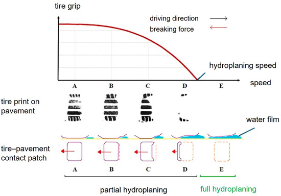
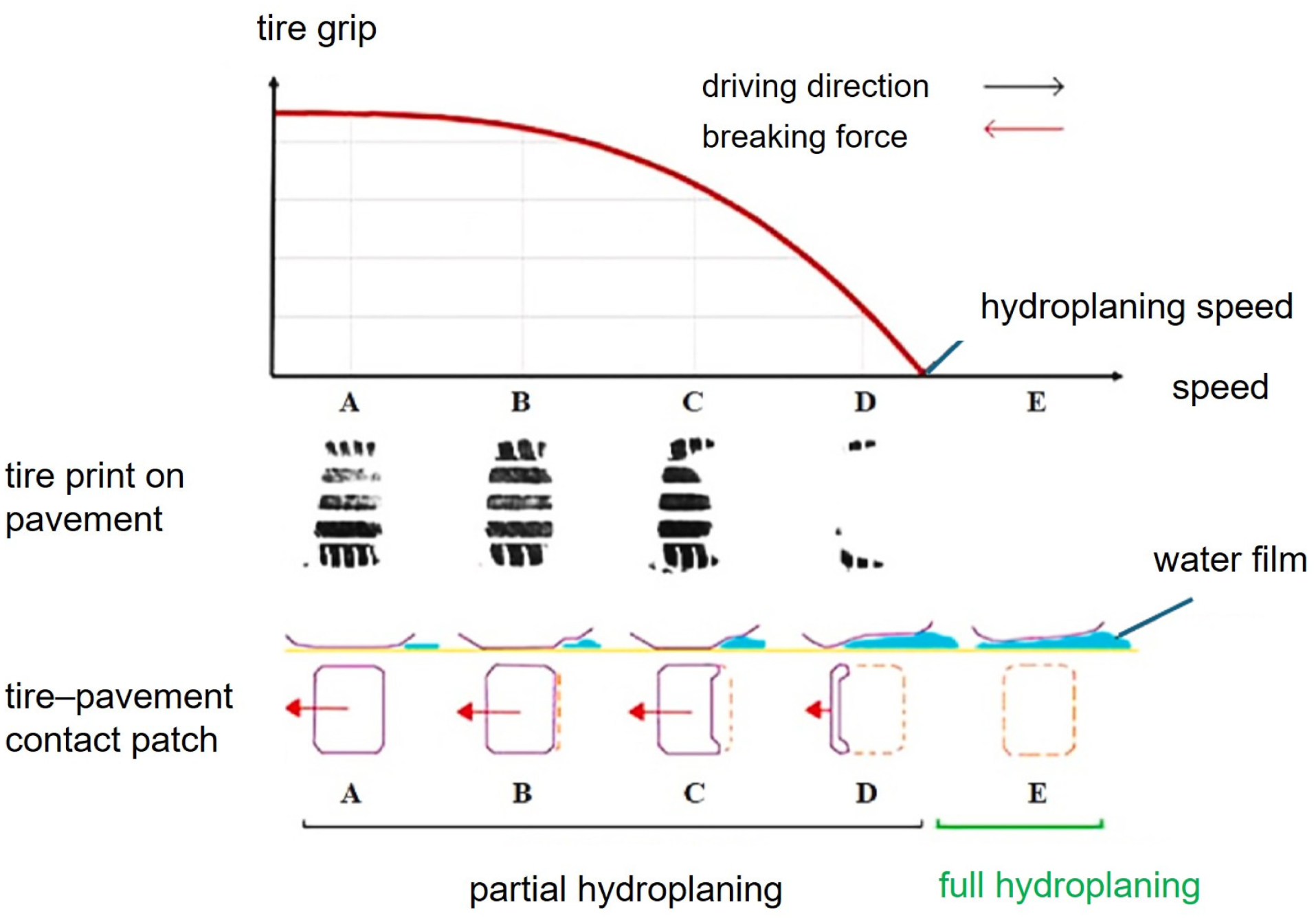
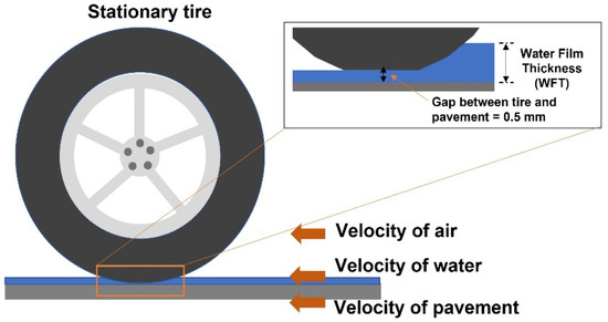
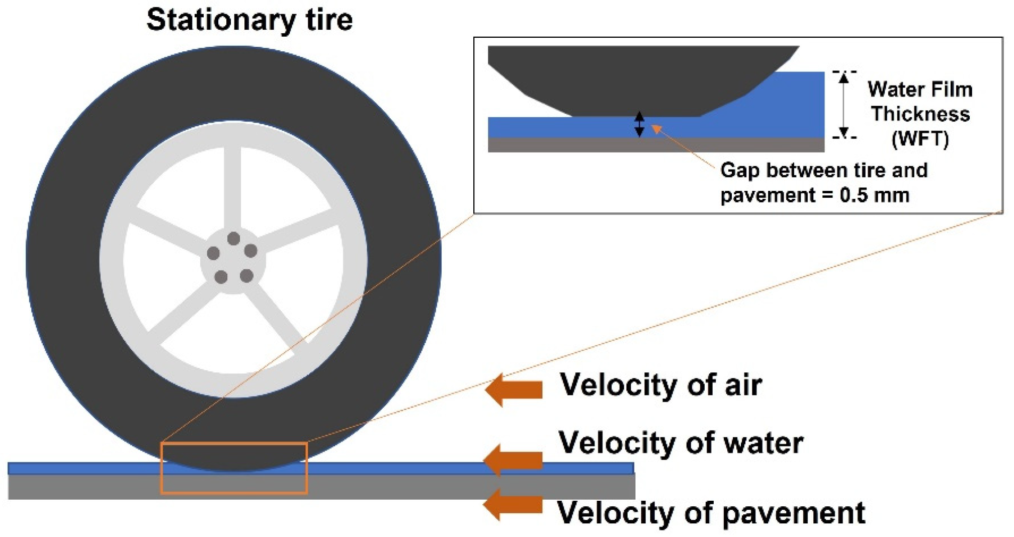
Ensuring the safe design and operation of highways requires an accurate understanding of the mechanisms governing vehicle hydroplaning, a phenomenon with significant implications for traffic safety under wet weather conditions. Hydroplaning occurs when a tire encounters a layer of water on the pavement and displaces the fluid rapidly enough to generate hydrodynamic pressure within the water film. As the vehicle speed increases, this pressure produces an uplift force on the tire, and fully developed hydroplaning begins when the resulting hydrodynamic lift balances the vertical wheel load, leading to a loss of solid contact between the tire and the pavement (Figure 1).

Figure 1. Schematic of incipient hydroplaning [1].

Early analytical and experimental studies sought to characterize hydroplaning by relating tire motion, fluid inertia, and wheel loading. Seminal experiments conducted by the National Aeronautics and Space Administration (NASA) on aircraft and automobile tires sliding over flooded, nominally smooth surfaces led to the well-known NASA hydroplaning equation [2,3]. Developed for smooth or ribbed tires on smooth pavements with a characteristic water film thickness of 7.62 mm, this empirical relationship relates the critical hydroplaning speed $V_p$ (km ${\mathrm{h}}^{-1}$) to the tire inflation pressure $p_t$ (kPa) as follows:

$$V_p=6.36\sqrt{p_t}.$$

(1)

Owing to its experimental basis and simplicity, the NASA equation is widely used as a conservative benchmark in both experimental and numerical studies, particularly for smooth tires on smooth pavements.

Subsequent experimental investigations have demonstrated that additional parameters, including tire footprint geometry, wheel load, and water film thickness, influence hydroplaning onset. These findings motivated the development of alternative empirical formulations, including the Texas Department of Transportation (TXDOT) model [4] and the PAVDRN computer model [5]. Building on this body of work, Gunaratne et al. [6] proposed the University of South Florida (USF) equation, which explicitly incorporates wheel load $W_L$ (N) and water film thickness WFT (mm), yielding Equation (2):

$$V_p=W_L^{0.2}{p}_t^{0.5}\left({\displaystyle \frac{0.82}{{\mathrm{W}\mathrm{F}\mathrm{T}}^{0.06}}}+0.49\right),$$

(2)

where the functional form is calibrated for locked-wheel tester tires and has been shown to be applicable to passenger vehicles with similar tire characteristics. Together, Equations (1) and (2), along with the TXDOT and PAVDRN equations, provide widely used empirical reference models for assessing hydroplaning risk under different pavement and hydraulic conditions.

Conducting laboratory experiments to replicate hydroplaning conditions is often impractical and expensive. Consequently, computational simulations have emerged as a cost-effective alternative for studying hydroplaning dynamics (see summary in Table 1). Over the years, a significant number of numerical models have been developed to investigate the parameters influencing hydroplaning, particularly those related to tire deformation, tread geometry, pavement macrotexture, and drainage characteristics [7,8,9,10,11,12,13,14,15,16,17,18,19,20,21,22,23,24,25,26,27]. Recent numerical contributions include the work of Aboelsaoud et al. [28], who used the coupled Eulerian–Lagrangian method in ABAQUS to investigate how the increased weight of electric vehicles relative to internal combustion engine vehicles affects hydroplaning, finding that the additional tire load can substantially reduce lift-to-load ratios, and Zeng et al. [29], who combined laser scanning of asphalt pavement surfaces with fluid–structure interaction simulations to evaluate the influence of pavement texture on hydroplaning, demonstrating that texture uniformity is a key factor in anti-skid performance under wet conditions. However, these studies have predominantly emphasized structural realism or pavement characteristics, while the hydrodynamics in the immediate vicinity of the tire are typically treated as a means to compute hydrodynamic lift rather than examined independently as a governing physical process.

Recent experimental studies have provided detailed insight into the complex, unsteady flow structures that develop within tire grooves under wet conditions [30], underscoring the richness of the tire–water interaction. Hermange et al. [31] used high-speed imaging through a transparent pavement section to quantify the progressive loss of tire–road contact area as a function of vehicle speed, water depth, tread depth, and inflation pressure, confirming that the water absorption capability of the tire tread is a key parameter governing hydroplaning onset. More recently, Vilsan et al. [32] developed a real-time hydroplaning risk estimation methodology using an intelligent tire system with an embedded force sensor to measure hydrodynamic lift within the tread groove, demonstrating that partial hydroplaning can be detected under shallow water conditions where the conventional water-wedge mechanism may not be present. However, none of the numerical modeling studies summarized in Table 1 have examined how turbulent hydrodynamics affect the hydroplaning speed predictions. Ong and Fwa [7,8] incorporated the k–ε turbulence closure in Reynolds-Averaged Navier–Stokes (RANS) simulations, and Nazari et al. [9] employed the shear stress transport (SST) k–ω closure within a fully coupled fluid–structure interaction framework. In these studies, turbulence modeling is included as part of the baseline formulation, but its specific influence on the predicted hydroplaning speed is not isolated or evaluated.

By contrast, many other numerical approaches treat the flow as laminar [2,10,11,12,13,14,15,16,32,33], employ depth-averaged or reduced hydrodynamic models [13,17,18,19], or use particle-based methods, such as smoothed particle hydrodynamics(SPH) or material point method(MPM), without explicit turbulence modeling [15,20,21]. Of the 23 numerical studies surveyed in Table 1, more than half (13) do not represent turbulence, instead treating the flow as laminar or inviscid. Thus, this practice is widespread despite Reynolds-number regimes where turbulent momentum transport may influence pressure buildup and hydrodynamic lift. Omitting turbulence representation in the vicinity of the tire, such as beneath the tire and near the leading edge, may bias pressure predictions and, in turn, lift-force estimates. Meanwhile, the influence of turbulence modeling on the hydrodynamics governing pressure buildup and lift, and therefore on the hydroplaning speed prediction, remains insufficiently investigated.

To address this gap, the overall objective of this study is to investigate the role of turbulence modeling in CFD-based prediction of the vehicle hydroplaning speed. The specific objectives are as follows: (1) to develop a three-dimensional RANS–VoF hydroplaning model with turbulence closure and to validate it against established experimentally derived hydroplaning equations; (2) to quantify the effect of turbulence on the predicted hydroplaning speed by comparing solutions obtained with and without turbulence closure; (3) to characterize the turbulent flow field beneath and in front of the tire to identify the physical mechanisms through which turbulence influences hydrodynamic lift; and (4) to assess whether a simplified rigid-tire, rectangular-footprint representation can capture the key hydrodynamic mechanisms governing lift generation and hydroplaning onset, bypassing the need to prescribe the true deformed tire footprint.

The remainder of this manuscript is organized as follows. The methodology section (Section 2) presents the governing equations, numerical model, geometry, boundary conditions, and simulation setup. Section 3 presents the model verification and hydroplaning speed predictions, followed by an analysis of the flow behavior near and beneath the tire. The final conclusions are provided in Section 4.

Table 1. Summary of the representative numerical studies of vehicle hydroplaning, emphasizing the numerical methods employed, whether turbulence effects are explicitly modeled, and flow regime assessment. Reynolds numbers are estimated as $Re=\rho VL/\mu$ with upstream water film thickness $L$, desnity $\rho$ = 998.2 kg/m³, and viscosity $\mu$ = 1.003 × 10⁻³ Pa·s.

Reference	Numerical Technique	Primary Application/Focus	Flow Treatment	Flow Regime Assessment
Cai et al. (2023) [22]	CFD–FEM FSI (CEL, ABAQUS)	Aircraft tire hydroplaning on grooved pavement.	Laminar formulation (no turbulence closure).	Re ≈ 613,000 at 80 m/s; flow expected to be turbulent.
Chen and Wang (2023) [23]	Pavement hydrology + CEL hydroplaning model	Spatiotemporal hydroplaning risk mitigation.	Laminar formulation (no turbulence closure).	Re ≈ 22,000–150,000 at 22–50 m/s; flow expected to be turbulent.
Chen et al. (2022) [24]	CFD (ANSYS Fluent; Ansys, Inc., Canonsburg, PA, USA; FVM)	Tire hydroplaning performance; tread effects.	Flow treatment not reported.	Re ≈ 20,000+ at 20 m/s; flow expected to be turbulent.
Cho et al. (2006) [25]	CFD (FVM, 3D patterned tire)	Hydroplaning of patterned tires.	Inviscid formulation (viscosity neglected, no turbulence closure).	Re ≈ 167,000 at 60 km/h; flow expected to be turbulent.
Deng et al. (2025) [10]	CFD–FEM FSI (CEL, ABAQUS)	Effects of driving conditions on hydroplaning.	Laminar formulation (no turbulence closure).	Re ≈ 112,000–173,000 at 70–85 km/h; flow expected to be turbulent.
Ding and Wang (2018) [11]	Tire–water–pavement interaction model (CEL, ABAQUS)	Hydroplaning risk on permeable pavements.	Laminar formulation (no turbulence closure).	Re ≈ 20,000–200,000 at 20–42 m/s; flow expected to be turbulent.
El-Sayegh and El-Gindy (2017) [20]	FEM–SPH coupling (Pam-Crash; ESI Group, Rungis, France))	Truck tire hydroplaning sensitivity.	Turbulence not modeled (SPH with molecular viscosity only).	Re ≈ 1,000,000–2,800,000 at 62–200 km/h with water depths 50–100 mm; flow expected to be turbulent.
Hermange et al. (2019) [21]	SPH–FE coupled FSI	Tire hydroplaning on rough ground.	Inviscid formulation (viscosity neglected, no turbulence closure).	Re ≈ 22,000 at 80 km/h with WFT 1 mm; flow expected to be turbulent.
Jeong and Jeong (2013) [33]	FEM (ALE, LS-DYNA; Ansys, Inc., Canonsburg, PA, USA); thin water estimation method	Hydroplaning and skid number estimation.	Laminar formulation (no turbulence closure).	Re ≈ 9000–390,000 at 40–140 km/h; flow expected to be turbulent at higher speeds.
Kim and Jeong (2010) [17]	FEM (tire) + reduced hydrodynamic solver (FDM/FVM)	Efficient prediction of hydroplaning speed for grooved and patterned tires.	Turbulence parameterized, not explicitly modeled.	Re ≈ 14,000–553,000 at 10–100 km/h with 5–20 mm WFT; flow expected to be turbulent at highway speeds.
Liu et al. (2019) [12]	Integrated tire–vehicle FEM (CEL, ABAQUS + CarSim; Mechanical Simulation Corporation, Ann Arbor, MI, USA)	Wet braking and hydroplaning.	Laminar formulation (no turbulence closure).	Re ≈ 11,000–220,000 at 40–80 km/h; flow expected to be turbulent.
Löwer et al. (2020) [13]	Analytical/physical model	Wet tire–road contact mechanics; pattern-dependent wet grip.	Inviscid primary flow; viscous losses via laminar Poiseuille profile; no turbulence closure.	Re ≈ 11,000–117,000 at 80–140 km/h with 0.5–3 mm water films; flow expected to be turbulent.
Nazari et al. (2020) [9]	CFD–FEM FSI	Hydroplaning potential prediction.	Turbulence modeled via closure (SST k–ω).	Re ≈ 89,000–186,000 at 17.9–24.5 m/s with 5–7.62 mm WFT; flow is turbulent; turbulence modeled (SST k–ω).
Ong (2006) [34]	CFD (2D and 3D, FVM + VoF)	Hydroplaning and skid resistance.	Turbulence modeled via closure (k–ε).	Re ≈ 85,000–233,000 at 40–110 km/h with 7.62 mm WFT; flow is turbulent; turbulence modeled.
Ong and Fwa (2006) [7]	CFD (FVM + VoF)	Transverse pavement grooving.	Turbulence modeled via closure (k–ε)	Re ≈ 85,000–233,000 at 40–110 km/h with 7.62 mm WFT; flow is turbulent; turbulence modeled
Ong and Fwa (2007) [8]	CFD + empirical modeling	Hydroplaning risk and skid resistance.	Turbulence modeled via closure (k–ε).	Re ≈ 85,000–233,000 at 40–110 km/h with 7.62 mm WFT; flow is turbulent; turbulence modeled.
Schulz et al. (2021) [18]	Integral control volume formulation (mass and momentum)	Water film thickness prediction and hydroplaning velocity.	Integral momentum balance; no turbulence closure, but turbulent effects may be implicitly captured through statistical analyses.	Re ≈ 224,000 at 100 km/h; flow expected to be turbulent at the tire.
Tao et al. (2022) [14]	CEL method (ABAQUS/Explicit; Dassault Systèmes SIMULIA, Johnston, RI, USA, FVM)	Hydroplaning of complex tread tires; effects of load, pressure, water film.	Mie–Grüneisen EOS with molecular viscosity only; no turbulence closure	Re ≈ 55,000–640,000 at 40–115 km/h with 5–20 mm water films; flow expected to be turbulent
Zheng et al. (2018) [19]	CEL method + VOF (ABAQUS/Explicit)	Tire–asphalt pavement adhesion; skid resistance on AC, SMA, OGFC.	Laminar N–S with molecular viscosity only; no turbulence closure implemented.	Re ≈ 11,000–140,000 at 20–100 km/h with 2–5 mm water films; flow expected to be turbulent.
Zhou et al. (2014) [26]	CFD (FVM + VoF, FLUENT)	Hydroplaning speed and influencing factors.	Turbulence modeled via closure (SST k–ω).	Re ≈ 250,000–277,000 at 90–100 km/h with 10 mm WFT; flow is turbulent.
Zhou et al. (2015) [27]	CFD (FVM + VoF, FLUENT)	Bionic riblet anti-hydroplaning.	Turbulence modeled via closure (SST k–ω).	Re ≈ 221,000 at 80 km/h with 10 mm WFT; flow is turbulent.
Zhou et al. (2025) [15]	Material Point Method (MPM)	Viscous hydroplaning mechanisms.	Laminar formulation (no turbulence closure).	Re ≈ 6000–30,000 at 26–30 m/s with 0.2–1.0 mm WFT; viscous hydroplaning regime, laminar treatment may be partially justified for thinnest films.
Zhu et al. (2017) [16]	FEM + CEL (ABAQUS FEA)	Pavement macrotexture and friction.	Laminar formulation (no turbulence closure).	Re ≈ 10,000–249,000 at 70–110 km/h with 0.5–10 mm WFT; flow expected to be turbulent for thicker films.

CFD: computational fluid dynamics; FEM: finite element method; FEA: finite element analysis; FE: finite element; FDM: finite difference method; FSI: fluid structure interaction; FVM: finite volume method; SPH: smoothed-particle hydrodynamics; CEL: coupled Eulerian–Lagrangian.

Table 1. Summary of the representative numerical studies of vehicle hydroplaning, emphasizing the numerical methods employed, whether turbulence effects are explicitly modeled, and flow regime assessment. Reynolds numbers are estimated as $Re=\rho VL/\mu$ with upstream water film thickness $L$, desnity $\rho$ = 998.2 kg/m³, and viscosity $\mu$ = 1.003 × 10⁻³ Pa·s.

Reference	Numerical Technique	Primary Application/Focus	Flow Treatment	Flow Regime Assessment
Cai et al. (2023) [22]	CFD–FEM FSI (CEL, ABAQUS)	Aircraft tire hydroplaning on grooved pavement.	Laminar formulation (no turbulence closure).	Re ≈ 613,000 at 80 m/s; flow expected to be turbulent.
Chen and Wang (2023) [23]	Pavement hydrology + CEL hydroplaning model	Spatiotemporal hydroplaning risk mitigation.	Laminar formulation (no turbulence closure).	Re ≈ 22,000–150,000 at 22–50 m/s; flow expected to be turbulent.
Chen et al. (2022) [24]	CFD (ANSYS Fluent; Ansys, Inc., Canonsburg, PA, USA; FVM)	Tire hydroplaning performance; tread effects.	Flow treatment not reported.	Re ≈ 20,000+ at 20 m/s; flow expected to be turbulent.
Cho et al. (2006) [25]	CFD (FVM, 3D patterned tire)	Hydroplaning of patterned tires.	Inviscid formulation (viscosity neglected, no turbulence closure).	Re ≈ 167,000 at 60 km/h; flow expected to be turbulent.
Deng et al. (2025) [10]	CFD–FEM FSI (CEL, ABAQUS)	Effects of driving conditions on hydroplaning.	Laminar formulation (no turbulence closure).	Re ≈ 112,000–173,000 at 70–85 km/h; flow expected to be turbulent.
Ding and Wang (2018) [11]	Tire–water–pavement interaction model (CEL, ABAQUS)	Hydroplaning risk on permeable pavements.	Laminar formulation (no turbulence closure).	Re ≈ 20,000–200,000 at 20–42 m/s; flow expected to be turbulent.
El-Sayegh and El-Gindy (2017) [20]	FEM–SPH coupling (Pam-Crash; ESI Group, Rungis, France))	Truck tire hydroplaning sensitivity.	Turbulence not modeled (SPH with molecular viscosity only).	Re ≈ 1,000,000–2,800,000 at 62–200 km/h with water depths 50–100 mm; flow expected to be turbulent.
Hermange et al. (2019) [21]	SPH–FE coupled FSI	Tire hydroplaning on rough ground.	Inviscid formulation (viscosity neglected, no turbulence closure).	Re ≈ 22,000 at 80 km/h with WFT 1 mm; flow expected to be turbulent.
Jeong and Jeong (2013) [33]	FEM (ALE, LS-DYNA; Ansys, Inc., Canonsburg, PA, USA); thin water estimation method	Hydroplaning and skid number estimation.	Laminar formulation (no turbulence closure).	Re ≈ 9000–390,000 at 40–140 km/h; flow expected to be turbulent at higher speeds.
Kim and Jeong (2010) [17]	FEM (tire) + reduced hydrodynamic solver (FDM/FVM)	Efficient prediction of hydroplaning speed for grooved and patterned tires.	Turbulence parameterized, not explicitly modeled.	Re ≈ 14,000–553,000 at 10–100 km/h with 5–20 mm WFT; flow expected to be turbulent at highway speeds.
Liu et al. (2019) [12]	Integrated tire–vehicle FEM (CEL, ABAQUS + CarSim; Mechanical Simulation Corporation, Ann Arbor, MI, USA)	Wet braking and hydroplaning.	Laminar formulation (no turbulence closure).	Re ≈ 11,000–220,000 at 40–80 km/h; flow expected to be turbulent.
Löwer et al. (2020) [13]	Analytical/physical model	Wet tire–road contact mechanics; pattern-dependent wet grip.	Inviscid primary flow; viscous losses via laminar Poiseuille profile; no turbulence closure.	Re ≈ 11,000–117,000 at 80–140 km/h with 0.5–3 mm water films; flow expected to be turbulent.
Nazari et al. (2020) [9]	CFD–FEM FSI	Hydroplaning potential prediction.	Turbulence modeled via closure (SST k–ω).	Re ≈ 89,000–186,000 at 17.9–24.5 m/s with 5–7.62 mm WFT; flow is turbulent; turbulence modeled (SST k–ω).
Ong (2006) [34]	CFD (2D and 3D, FVM + VoF)	Hydroplaning and skid resistance.	Turbulence modeled via closure (k–ε).	Re ≈ 85,000–233,000 at 40–110 km/h with 7.62 mm WFT; flow is turbulent; turbulence modeled.
Ong and Fwa (2006) [7]	CFD (FVM + VoF)	Transverse pavement grooving.	Turbulence modeled via closure (k–ε)	Re ≈ 85,000–233,000 at 40–110 km/h with 7.62 mm WFT; flow is turbulent; turbulence modeled
Ong and Fwa (2007) [8]	CFD + empirical modeling	Hydroplaning risk and skid resistance.	Turbulence modeled via closure (k–ε).	Re ≈ 85,000–233,000 at 40–110 km/h with 7.62 mm WFT; flow is turbulent; turbulence modeled.
Schulz et al. (2021) [18]	Integral control volume formulation (mass and momentum)	Water film thickness prediction and hydroplaning velocity.	Integral momentum balance; no turbulence closure, but turbulent effects may be implicitly captured through statistical analyses.	Re ≈ 224,000 at 100 km/h; flow expected to be turbulent at the tire.
Tao et al. (2022) [14]	CEL method (ABAQUS/Explicit; Dassault Systèmes SIMULIA, Johnston, RI, USA, FVM)	Hydroplaning of complex tread tires; effects of load, pressure, water film.	Mie–Grüneisen EOS with molecular viscosity only; no turbulence closure	Re ≈ 55,000–640,000 at 40–115 km/h with 5–20 mm water films; flow expected to be turbulent
Zheng et al. (2018) [19]	CEL method + VOF (ABAQUS/Explicit)	Tire–asphalt pavement adhesion; skid resistance on AC, SMA, OGFC.	Laminar N–S with molecular viscosity only; no turbulence closure implemented.	Re ≈ 11,000–140,000 at 20–100 km/h with 2–5 mm water films; flow expected to be turbulent.
Zhou et al. (2014) [26]	CFD (FVM + VoF, FLUENT)	Hydroplaning speed and influencing factors.	Turbulence modeled via closure (SST k–ω).	Re ≈ 250,000–277,000 at 90–100 km/h with 10 mm WFT; flow is turbulent.
Zhou et al. (2015) [27]	CFD (FVM + VoF, FLUENT)	Bionic riblet anti-hydroplaning.	Turbulence modeled via closure (SST k–ω).	Re ≈ 221,000 at 80 km/h with 10 mm WFT; flow is turbulent.
Zhou et al. (2025) [15]	Material Point Method (MPM)	Viscous hydroplaning mechanisms.	Laminar formulation (no turbulence closure).	Re ≈ 6000–30,000 at 26–30 m/s with 0.2–1.0 mm WFT; viscous hydroplaning regime, laminar treatment may be partially justified for thinnest films.
Zhu et al. (2017) [16]	FEM + CEL (ABAQUS FEA)	Pavement macrotexture and friction.	Laminar formulation (no turbulence closure).	Re ≈ 10,000–249,000 at 70–110 km/h with 0.5–10 mm WFT; flow expected to be turbulent for thicker films.

CFD: computational fluid dynamics; FEM: finite element method; FEA: finite element analysis; FE: finite element; FDM: finite difference method; FSI: fluid structure interaction; FVM: finite volume method; SPH: smoothed-particle hydrodynamics; CEL: coupled Eulerian–Lagrangian.

2. Methodology

A three-dimensional, Reynolds-averaged multifluid (air–water) model was developed to simulate hydroplaning of a smooth tire over a flooded, nominally smooth pavement. Simulations were performed both with and without turbulence closure, and the realizable k–ε and SST k–ω models were considered under the same geometric and hydraulic conditions. For a uniform water film thickness of 7.62 mm, consistent with Equation (1), and a 0.5 mm water gap between the tire and the pavement, also consistent with Equation (1), the model was used to quantify the effect of including turbulence modeling on the predicted hydroplaning speed as a function of tire inflation pressure (100–300 kPa), relative to a purely laminar formulation. The resulting predictions were compared with the NASA [2,3], TXDOT [4], PAVDRN [5], and USF [6] empirical formulations.

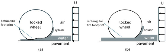
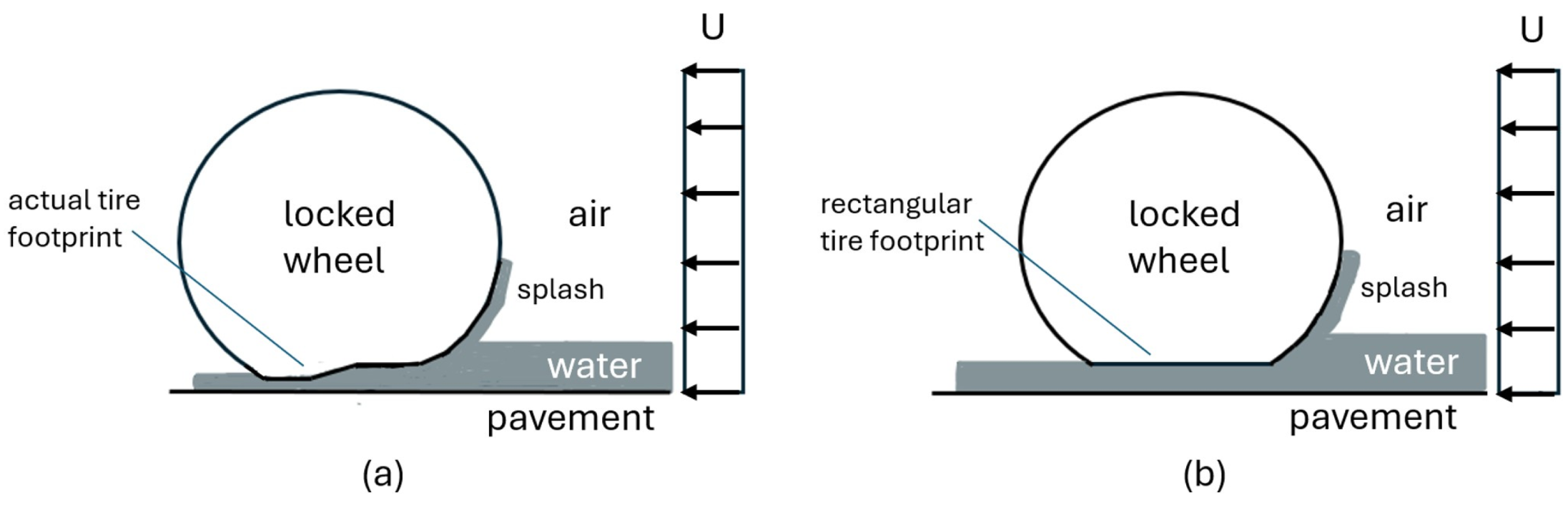
In addition, unlike earlier simplified CFD studies [7,8] that prescribe a measured deformed tire footprint, our model represents the tire footprint as a rectangular patch whose area is determined from the tire load and inflation pressure (Figure 2). This simplification eliminates the need to measure or assume a specific deformation profile, isolates the hydrodynamic response from uncertainties in tire deformation, and still blocks and redirects the oncoming water film in a way that preserves the essential lift–load balance governing hydroplaning. As a result, the simplified footprint enables a clean characterization of shear-dominated turbulence in the under-tire gap and stagnation driven turbulence at the front of the tire, while retaining the ability to reproduce the hydroplaning-speed–versus–inflation-pressure relationship in Equation (1). Accordingly, the present geometry should be interpreted as a first-order hydrodynamic surrogate intended to capture the integrated lift mechanism and hydroplaning onset, rather than the exact pointwise pressure field of a deformed curved tire.

Figure 2. Sketches of the flow configuration (in the tire-fixed frame) highlighting (a) the tire footprint measured in physical experiments [2,3] and (b) the idealized rectangular footprint (bottom patch) adopted in this study. In (b), the rectangular footprint area can be obtained from the tire mechanics as $A=W/p_t$, where $W$ is the tire load and $p_t$ is the tire inflation pressure. The speeds of the far field air and water film and the pavement are all equal and denoted as U.

2.1. Model Flow Equations

The fluid flow considered here is described using the incompressible continuity equation, obtained from mass conservation, as given in Equation (3), together with the Navier–Stokes equations for an incompressible Newtonian fluid, as given in Equation (4):

$${\displaystyle \frac{\partial u_i}{\partial x_i}}=0$$

(3)

$${\displaystyle \frac{\partial u_i}{\partial t}}+u_j{\displaystyle \frac{\partial u_i}{\partial x_j}}=-{\displaystyle \frac{1}{\rho }}{\displaystyle \frac{\partial P}{\partial x_i}}+\nu {\displaystyle \frac{{\partial }^2{u}_i}{\partial x_j^2}}+g_i$$

(4)

In these equations (e.g., Batchelor [35]), the $i$-th component of the fluid velocity is $u_i$, the spatial directions are denoted by $x_1,x_2$, and $x_3$, pressure is $P$, water density is $\rho$, time is $t$, and the molecular kinematic viscosity is $\nu$.

The gravitational acceleration component is $g_i$. In the VoF framework used here, the density in Equation (4) varies spatially according to the volume fraction, $\rho =\gamma {\rho }_{water}+\left(1-\gamma \right){\rho }_{air}$, where $\gamma$ is the volume fraction of water, so that the body force term couples gravity to the air–water interface dynamics. For the hydroplaning conditions considered here, the gravitational body forces are small relative to the inertial and pressure forces: for example, at a hydroplaning speed of 25 m/s with a 10 mm water film, the dynamic pressure is $\rho V^2/2$ ≈ 312 kPa, whereas the hydrostatic pressure is $\rho gh$ ≈ 0.1 kPa, a ratio of roughly 3000:1.

Solving the continuity and Navier–Stokes equations for turbulent flows is challenging because the velocity fluctuations must be resolved across all relevant spatial and temporal scales. In a direct numerical simulation (DNS), the full spectrum of the turbulent scales is captured on a sufficiently fine mesh, yielding a complete description of the flow field without any turbulence closure or model. However, the computational cost of the DNS is prohibitive for most engineering applications due to the extremely large number of elements required. A large-eddy simulation (LES), which resolves the larger energy-carrying eddies while modeling the smaller scales, also remains computationally expensive for the Reynolds numbers of interest here.

A fully three-dimensional, transient, free-surface simulation with a thin under-tire water film at practical Reynolds numbers is already very demanding. Performing an LES or DNS for the parameter space considered here (tire load, inflation pressure, water film thickness, vehicle speed) would currently be prohibitive.

Given the above computational constraints, we adopt the Reynolds-averaged Navier–Stokes (RANS) equations and associated turbulence closures for our hydroplaning model. Quantification of the average influence of the turbulence on the hydroplaning speed can then be carried out by comparing the results obtained with the RANS equations directly with the corresponding results obtained with the laminar (i.e., having no turbulence model/effects) formulation (Equations (3) and (4)) on the same grid. Note, however, that the LES or DNS should be pursued in future studies to understand the fine-scale turbulent structures underneath and around the tire. RANS studies, such as the present study, could be used to guide and help provide initial conditions for the LES or DNS.

The RANS equations are derived from time averaging which can be used to decompose the flow into a mean component and a turbulent component. If $t_i$ is the integral time scale (i.e., the time scale characteristic of the turbulence), over some time scale longer than $t_i$, the velocity is decomposed as follows:

$$u_i\left(x_j,t\right)={\overline{u}}_i\left(x_j,t\right)+u_i^{\prime }\left(x_j,t\right),$$

(5)

where $u_i\left(x_j,t\right)$ is the instantaneous $i$-th component of the velocity and where the mean velocity is as follows:

$${\overline{u}}_i\left(x_j,t\right)={\displaystyle \frac{1}{t_i}}{\int }_t^{t+t_i}{u}_i\left(x_j,\tau \right)d\tau$$

(6)

and $u_i^{\prime }\left(x_j,t\right)$ is the fluctuating (turbulent) component, using indicial notation.

The set of Reynolds-averaged continuity and RANS equations that can be obtained from averaging Equations (3) and (4), while utilizing the Reynolds decomposition in Equation (5), is as follows:

$${\displaystyle \frac{\partial {\overline{u}}_i}{\partial x_i}}=0$$

(7)

$${\displaystyle \frac{\partial {\overline{u}}_i}{\partial t}}+{\overline{u}}_k{\displaystyle \frac{\partial {\overline{u}}_i}{\partial x_k}}=-{\displaystyle \frac{1}{\rho }}{\displaystyle \frac{\partial \overline{P}}{\partial x_i}}+\nu {\displaystyle \frac{{\partial }^2{\overline{u}}_i}{\partial x_j^2}}+{\displaystyle \frac{\partial R_{ik}}{\partial x_k}}+g_i$$

(8)

where $R_{ik}=-\overline{u_i^{\prime }{u}_k^{\prime }}$ is the Reynolds stress tensor. This stress appears in the system of equations due to the averaging procedure, and accounts for the effect of the turbulence on the mean flow. Note that the turbulent fluctuation $u_i^{\prime }$ is not explicitly computed, as only the mean velocity ${\overline{u}}_i$ is available from the solution of Equations (7) and (8), thus the Reynolds stress has to be modeled or approximated to close the system of equations. Closure is facilitated through turbulence modeling as follows:

$$R_{ik}=-\overline{u_i^{\prime }{u}_k^{\prime }}=2{\nu }_t{\overline{S}}_{ik}-{\displaystyle \frac{2}{3}}k{\delta }_{ik}$$

(9)

where ${\nu }_t$ is the turbulent (eddy) viscosity, $k$ is the turbulence kinetic energy, and ${\overline{S}}_{ik}$ is defined as follows:

$${\overline{S}}_{ik}={\displaystyle \frac{1}{2}}\left({\displaystyle \frac{\partial {\overline{u}}_i}{\partial x_i}}+{\displaystyle \frac{\partial {\overline{u}}_k}{\partial x_j}}\right)$$

(10)

where ${\overline{S}}_{ik}$ is the mean strain-rate tensor and ${\delta }_{ik}$ is the Kronecker delta. Exclusion of the divergence of $R_{ik}$ from Equation (8), reverts Equations (7) and (8) to the laminar Equations (3) and (4).

2.2. Turbulence Models

Due to the broad physical modeling capabilities it possesses to model turbulent flows, ANSYS FLUENT 2023 R2 (Ansys, Inc., Canonsburg, PA, USA) [36,37] has been chosen for the model development in this study. Two turbulence models, namely the k–ε and k–ω models, are widely utilized in industrial CFD due to their robustness and accuracy [37]. Particularly, the realizable version of the k–ε model and the shear stress transport (SST) version of the k–ω model are favored for their excellent performance in flow scenarios involving boundary layers subjected to significant pressure gradients [38]. Consequently, the selection of these two models is expected to effectively capture the hydroplaning conditions.

The realizable k–ε model transport equations are as follows:

$${\displaystyle \frac{\partial k}{\partial t}}+{\overline{u}}_j{\displaystyle \frac{\partial k}{\partial x_j}}={\displaystyle \frac{\partial }{\partial x_j}}\left[\left(\nu +{\displaystyle \frac{{\nu }_t}{{\sigma }_k}}\right){\displaystyle \frac{\partial k}{\partial x_j}}\right]+P_k-\epsilon$$

(11)

$${\displaystyle \frac{\partial \epsilon }{\partial t}}+{\overline{u}}_j{\displaystyle \frac{\partial \epsilon }{\partial x_j}}={\displaystyle \frac{\partial }{\partial x_j}}\left[\left(\nu +{\displaystyle \frac{{\nu }_t}{{\sigma }_{\epsilon }}}\right){\displaystyle \frac{\partial \epsilon }{\partial x_j}}\right]+C_{1\epsilon }S\epsilon -C_{2\epsilon }{\displaystyle \frac{{\epsilon }^2}{k+\sqrt{\nu \epsilon }}}$$

(12)

where $k$ is the turbulent kinetic energy (TKE), $\epsilon$ is TKE dissipation rate, and $P_k$ is the production of TKE. The production of TKE by mean shear $P_k$ is defined as follows:

$$P_k=2\rho {\nu }_t{\overline{S}}_{ij}{\overline{S}}_{ij}$$

(13)

where the mean strain-rate tensor is defined in Equation (10), and $S={\left(2{\overline{S}}_{ij}{\overline{S}}_{ij}\right)}^{1/2}$ is the norm of the mean strain-rate tensor. The TKE and TKE dissipation rate are related through the eddy-viscosity (${\nu }_t$) relation as follows:

$${\nu }_t=C_{\mu }{\displaystyle \frac{k^2}{\epsilon }}$$

(14)

Constant values are $C_{1\epsilon }=1.44$, $C_{2\epsilon }=1.9,$ ${\sigma }_k=1$, and ${\sigma }_{\epsilon }=1.2$, and the expression for $C_{\mu }$ can be found in Ref. [38].

While the standard k–ω model is superior to the k–ε model for near-wall treatment, k–ω suffers from a sensitivity to free-stream turbulence intensity at the flow inlets. To mitigate this, the SST k–ω model utilizes a blending function to transition between two formulations: it adopts a k–ε behavior in the free-stream to ensure stability against inlet conditions, while reverting to the standard k–ω formulation near the wall. This allows for direct integration through the viscous sublayer without the need for wall functions, which the standard k–ε model typically requires.

The SST k–ω model transport equations are defined as follows:

$${\displaystyle \frac{\partial k}{\partial t}}+{\overline{u}}_j{\displaystyle \frac{\partial k}{\partial x_j}}={\displaystyle \frac{\partial }{\partial x_j}}\left[\left(\nu +{\displaystyle \frac{{\nu }_t}{{\sigma }_k}}\right){\displaystyle \frac{\partial k}{\partial x_j}}\right]+\widetilde{P_k}-Y_k$$

(15)

$${\displaystyle \frac{\partial \omega }{\partial t}}+{\overline{u}}_j{\displaystyle \frac{\partial \omega }{\partial x_j}}={\displaystyle \frac{\partial }{\partial x_j}}\left[\left(\nu +{\displaystyle \frac{{\nu }_t}{{\sigma }_{\omega }}}\right){\displaystyle \frac{\partial \omega }{\partial x_j}}\right]+P_{\omega }-Y_{\omega }$$

(16)

where $\omega$ is the specific dissipation rate, $\widetilde{P_k}$ and $P_{\omega }$ are production terms, and $Y_k$ and $Y_{\omega }$ are dissipation terms. The eddy viscosity is modeled as follows:

$${\nu }_t={\displaystyle \frac{a_{1}k}{max\left(a_1\omega ,\hspace{0.17em}S{F}_2\right)}}\hspace{1em}$$

(17)

where $a_1=0.31,S={\left(2{\overline{S}}_{ij}{\overline{S}}_{ij}\right)}^{1/2}$ is the norm of the mean strain-rate tensor and $F_2$ is an auxiliary relation defined as follows:

$$F_2=\mathrm{t}\mathrm{a}\mathrm{n}\mathrm{h}\left({\left[\mathrm{m}\mathrm{a}\mathrm{x}\left({\displaystyle \frac{2\sqrt{k}}{{\beta }^{\ast }\omega d}},\hspace{0.17em}{\displaystyle \frac{500\nu }{d^2\omega }}\right)\right]}^2\right)\hspace{1em}$$

(18)

with ${\beta }^{\ast }=9/100$ and $d$ is the wall-normal distance to the closest no-slip wall or surface. The interested reader may find expressions for ${\sigma }_k$, ${\sigma }_{\omega }$, $\widetilde{P_k},Y_k,$ $P_{\omega }$ and $Y_{\omega }$ in Ref. [36].

Regarding near-wall treatment, the realizable k–ε model was solved with standard wall functions, whereas the SST k–ω model was solved with FLUENT’s correlation-based near-wall treatment, which is a y+-insensitive formulation [36,37].

2.3. Volume of Fluid (VoF) Method

Utilizing the VoF method facilitates tracking the air–water interface in hydroplaning by calculating the volume fractions of the two fluids as field variables [36]. The density and viscosity are defined as follows:

$$\rho ={\rho }_1\gamma +{\rho }_2\left(1-\gamma \right)$$

(19)

$$\mu ={\mu }_1\gamma +{\mu }_2\left(1-\gamma \right)$$

(20)

where ${\rho }_1$ and ${\rho }_2$ are the densities of air and water, ${\mu }_1$ and ${\mu }_2$ are the dynamic viscosities of air and water, respectively, and $\gamma$ is the volume fraction of the water. The VoF method keeps track of the volume fraction occupied by the two fluids. The fluid corresponding to pure water is at grid cells with $\gamma =1$; the fluid corresponding to air is at cells with $\gamma =0$. At cells where $0<\gamma <1$, the fluid is a mixture of water and air with the middle of the interface between the two fluids corresponding to $\gamma =0.5$. The volume fraction was tracked via solution of a transport equation for $\gamma$, which corresponds to the conservation of mass equation of water, as follows:

$${\displaystyle \frac{\partial \gamma }{\partial t}}+{\overline{u}}_i{\displaystyle \frac{\partial \gamma }{\partial x_i}}=0$$

(21)

where the fluid velocity $u_i$ corresponds to the water velocity at grid cells where $\gamma =1$, $u_i$ is the velocity of the air at cells where $\gamma =0$, and $u_i$ is the velocity of the water–air mixture at cells where $0<\gamma <1$.

It should be recognized that phase change is neglected because, under typical hydroplaning conditions, a given segment of the water film directly under and around the tire remains in this vicinity for only a few milliseconds, the water and pavement temperatures remain far below boiling, and evaporation over such short times is negligible compared with the water film thickness. As a result, the dominant physics are inertial and pressure-driven and are well captured by an incompressible two-fluid (air–water) VoF formulation without requiring mass exchange across the air and water.

2.4. Tire–Water–Air Model

2.4.1. Conceptualization of the Model

Vehicle hydroplaning can be visualized with a tire (in locked-wheel mode) sliding on the stationary rigid pavement covered with water. Alternatively, this scenario can be viewed by considering the moving tire as the reference illustrated in Figure 3. The latter has been considered in model development. The gap between the bottom tire rectangular patch and the pavement has been taken as 0.5 mm, consistent with the nominal tire–pavement gaps considered in previous models (e.g., [7,8,34]) and laboratory measurements [2,3]. This value was not introduced as a tunable calibration parameter; rather, it was adopted as a physically constrained baseline derived from prior hydroplaning laboratory experiments. The NASA-based hydroplaning profiles reported by Horne and Joyner [2] involve a non-uniform under-tire clearance that decreases to approximately 0.5 mm near the downstream end of the hydroplaning region, and the present model preserves this minimum observed passage height. A further basis for the 0.5 mm scale is provided by Ong [34], who noted that pavement macrotexture, defined as beginning at approximately 0.5 mm, provides (together with the tire tread) the principal escape channels for rainwater trapped in the contact patch. In the present smooth-tire, smooth-pavement model, the prescribed 0.5 mm gap should therefore be interpreted as a simplified minimum drainage/clearance surrogate rather than an unconstrained fitted constant. Simulations were conducted for various values of the water film thickness (WFT) upstream of the tire.

Figure 3. Conceptualization of hydroplaning model. Note that the tire is lifted from the pavement by the water film (denoted in blue) during the steady-state hydroplaning considered here.

2.4.2. Material Properties

For the current study, two fluids, air and water, have been considered at a reference temperature of 298 K. The densities of air and water are 1.225 kg/m³ and 998.2 kg/m³, respectively, while the dynamic viscosities are 1.7894 × 10⁻⁵ and 1.003 × 10⁻³ Pa·s, respectively. The surface tension coefficient was set as $\sigma =0.072\mathrm{N}$/m, which is the standard value for an air–water interface at 20–25 °C.

2.4.3. Geometry of the Tire Model and Computational Domain

Modeling the entire domain around the tire proves to be computationally expensive. Particularly at incipient hydroplaning, the lift on the tire results from the hydrodynamic pressure generated by stagnated water at the tire’s front in bow waves, and water penetrating the tire–pavement contact area. Although the lift force from the surrounding air is minimal compared to water, both fluids must be incorporated in the model to track the air–water interface and water splashing against the tire. Therefore, focusing on the domain surrounding the bottom half of the tire, where water plays a significant role, is adequate for accurately predicting the water and air flow around the tire. This domain, symmetrical with respect to the tire’s vertical plane, is modeled only on one side to reduce computational effort.

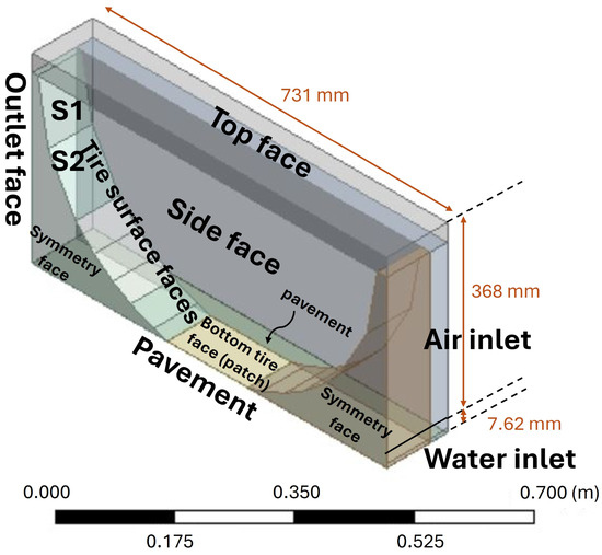
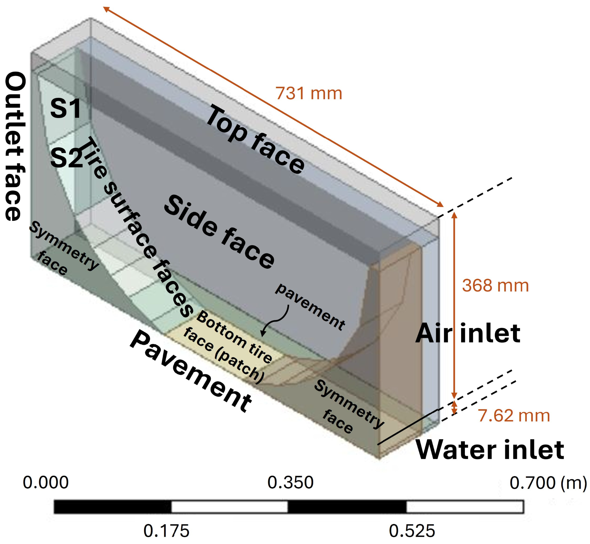
Figure 4 shows the 0.7 m-diameter tire model and the geometry of the computational domain. As illustrated, two velocity inlets have been located upstream with an air inlet height of 368 mm and a water inlet height (or the water film thickness) of 7.62 mm. This water inlet height was adjusted to analyze different cases of interest. Both inlets have a width of 125 mm. The pavement length is 731 mm and the gap between the pavement and the tire is kept at 0.5 mm, the latter following earlier numerical experiments [7,8,34], as noted earlier. In the current study, a mesh sensitivity analysis was carried out for a bottom tire face (patch) area of 0.03 m². The location of the patch is illustrated in Figure 4. The rest of the results presented were averaged over cases with bottom patch areas of 0.03, 0.035, and 0.04 m².

Figure 4. Geometry of the model. The tire diameter is 0.7 m. Water occupies the gap between the pavement and the bottom tire contact patch (i.e., the bottom tire face). Tire surface faces S1 through S7 refer to faces on the inlet side (leading edge) of the tire, but have been shown on the back (downstream) side of the tire for ease of labeling. The bottom tire patch corresponds to S8.

In the simplified representation of the tire (Figure 2b and Figure 4), the rectangular footprint (patch) area $A_{\mathrm{p}\mathrm{a}\mathrm{t}\mathrm{c}\mathrm{h}}$ is related to the tire load $W$ and inflation pressure $p_t$ by the usual tire–mechanics relation $A_{\mathrm{p}\mathrm{a}\mathrm{t}\mathrm{c}\mathrm{h}}=W/p_t$ when the tire is in contact with the pavement. In classical tire mechanics, $W$ and $p_t$ are known, and $A_{\mathrm{p}\mathrm{a}\mathrm{t}\mathrm{c}\mathrm{h}}$ is inferred from this relation. In the present CFD formulation, however, $A_{\mathrm{p}\mathrm{a}\mathrm{t}\mathrm{c}\mathrm{h}}$ must be specified in advance to define the computational domain, while the effective inflation pressure $p_t$ is only known a posteriori from the simulated (computed) hydrodynamic lift. To avoid this apparent circularity, we treat $A_{\mathrm{p}\mathrm{a}\mathrm{t}\mathrm{c}\mathrm{h}}$ as a parameter and perform CFD simulations for three values: 0.03, 0.035, and $0.04$ m². For each case, the lift at hydroplaning, $F_L$, obtained from the CFD simulations, is equated to the tire load $W$, and the corresponding effective inflation pressure is obtained as $p_t=W/A_{\mathrm{p}\mathrm{a}\mathrm{t}\mathrm{c}\mathrm{h}}$. For the range of effective inflation pressures computed in this study (50–300 kPa), these areas correspond to tire loads $W=A_{\mathrm{p}\mathrm{a}\mathrm{t}\mathrm{c}\mathrm{h}}{p}_t$ in the range 1.5–12 kN. This interval encompasses typical per-tire loads for passenger cars and sport utility vehicles (approximately 3–7 kN), with the lower and upper ends representing lightly and heavily loaded conditions, respectively. The footprint areas selected are therefore representative of realistic highway vehicles, and the hydroplaning-speed–versus–$p_t$ and hydroplaning-speed–versus–WFT curves reported in the Section 3 below are obtained by averaging over these three physically plausible patch areas (except for the mesh-convergence analysis, which was performed with $A_{\mathrm{p}\mathrm{a}\mathrm{t}\mathrm{c}\mathrm{h}}=0.03$ m², as noted earlier).

It is noted that the effective inflation pressure used in this study is inferred a posteriori from the CFD-computed hydrodynamic lift, rather than being a directly measured physical input, as in the empirical equations, where it is simply the gauge pressure of the air inside the tire. The comparison with empirical hydroplaning formulas should therefore be interpreted as a comparison at matched values of effective pressure under lift–load equilibrium. This is acknowledged as a modeling limitation; however, the predicted hydroplaning-speed curves are remarkably insensitive to moderate variations in the footprint area, as shown in the Section 3, indicating that treating the footprint area as a geometric input does not introduce material bias into the comparison over the realistic range examined here.

A notable alteration in the tire geometry involves substituting the curved tire surface with multiple planar surfaces labeled as S1, S2 …, S7 (Figure 4). By incorporating known inclinations (α) of the planar surfaces, computing the vertical component of the hydrodynamic force responsible for the tire lift proved to be more straightforward in the solution process.

2.4.4. Boundary Conditions

As illustrated in Figure 4, two velocity inlets have been located upstream, namely the air inlet and the water inlet. Water is to flow 286 mm from the inlet before encountering the tire, resulting in sufficient space in the front of the tire to allow stagnation of water in the form of waves. The stagnating water is eventually diverted towards the side face of the domain or forced through the gap between the tire and the pavement, where it can also be diverted towards the side face.

Following the computational domain in Figure 4, the inlet boundaries have been modeled as velocity inlets. Turbulent intensity and the turbulent viscosity-to-molecular viscosity ratio (non-dimensional) at the boundaries were specified as 3% (of the prescribed inlet velocity) and 8%, respectively [36,37]. The predicted hydroplaning speed is insensitive to the precise values of these inlet turbulence parameters, because the pavement, water film, and air at the inlet all translate at the same velocity (recall Figure 3), producing no velocity gradient and therefore no shear production of turbulence between the inlet boundary and the leading edge of the tire. Any turbulence specified at the inlet therefore decays monotonically before reaching the tire. Turbulence is generated locally only once the flow encounters the stationary tire surface, which introduces the shear responsible for the elevated turbulence kinetic energy observed in the under-tire gap and leading edge regions, as analyzed in the Section 3.

The pavement has been modeled as a moving smooth surface (see the pavement conditions subsection below for further discussion on this smoothness property) with the same velocity as that of the air and water at the inlet. The pavement has been specified as one of no slip in relation to the fluid. The stationary tire has been specified as a no slip surface with small roughness (see Section 2.4.5 below). With these conditions, a boundary layer is expected between the water and the tire below the bottom tire patch; no boundary layer is expected between the water and the pavement. The flow variables on the top, outlet, and side faces of the domain can be rationally approximated to be pressure outlets with pressures set to the atmospheric value. Due to symmetry, the normal velocity and the normal gradients of all variables are zero at the central vertical plane (symmetry face) of the domain.

The distances chosen to locate the boundaries were checked to verify they are adequately apart from the tire, since placing them too close may cause numerical inaccuracies in calculating the hydrodynamic pressures [34]. Several test cases were conducted with different domain lengths, and it was found that the steady-state volume fractions of air and water predicted via the VoF method exhibited the same behavior. Thus, the location of the boundaries chosen did not have an adverse effect on the results.

2.4.5. Representation of the Tire

In addition to considering a tire with a rectangular bottom patch, as discussed earlier, the tire surface is taken to be smooth. The reasons for choosing a tire with no texture can be summarized as follows.

Standard practice in pavement skid testing: Pavement skid testers, widely used for friction measurements, typically employ smooth tires, aligning with the development context of the NASA equation (Equation (1)) under such conditions [2,3]. The use of smooth tires is critical because it focuses on assessing the pavement conditions essential for the safe operation of aircraft and vehicles. Incorporating tire texture can complicate the results by introducing additional variables that are not related to the pavement’s inherent skid resistance [39,40].

Sensitivity to pavement macrotexture: Smooth tires are more sensitive to the macrotexture of the pavement, which is a crucial parameter in evaluating skid resistance. The locked-wheel tester, a common device used in these tests, uses smooth tires to measure the frictional force and skid number, providing a clear and consistent measure of the pavement’s performance under wet conditions. Ribbed or treaded tires, on the other hand, are more sensitive to microtexture changes, which can vary significantly and add complexity to the interpretation of results [39].

Worst-case scenario representation: Smooth tires, characterized by minimal traction and the absence of water escape channels, represent the most challenging scenario for tire–pavement interaction. This creates a worst-case scenario that helps in understanding the maximum potential for hydroplaning. Therefore, our study was focused on this worst-case scenario to ensure that model results are robust and reliable under the most adverse conditions.

Simplifications: The elimination of variables such as tire tread, depth, and pattern allows us to explore the possibility to isolate the effects of hydrodynamics underneath the tire and the variables related to it. However, it is important to acknowledge that even “smooth tires” possess a certain degree of surface roughness, hence using a reasonably low roughness value for the tire surface would be prudent. To account for this, a roughness height of one hundredth of a millimeter was introduced to our tire model, maintaining compliance with the smoothness condition while representing real-world tire surfaces more accurately.

2.4.6. Representation of Pavement Surface

Water within macrotexture asperities in the pavement can influence the flow within the water film above the pavement surface through mass and momentum interchange. A full representation of this process is outside of the scope of the present study; thus, the pavement is assumed to be smooth, consistent with the experiments that led to the NASA hydroplaning equation (Equation (1)). Furthermore, the microtexture in a pavement is generated due to the small-scale texture of the aggregate and primarily controls the adhesion between the tire and the road. Hence, pavement microtexture does not play a pivotal part in hydroplaning.

2.5. Computational Details

2.5.1. Steady-State Solution Strategy

The equations for the coupled Reynolds-averaged continuity and momentum in Equations (7)–(10), together with those for the turbulence model in Equations (11)–(18) and the VoF model in Equations (19)–(21), are integrated in time from a prescribed initial condition. Because the flow is driven by time-independent forcing (i.e., time-independent boundary conditions), as in the present study, time integration leads to a steady-state solution. Our primary interest is the pressure exerted by the flow on the tire for a given inlet/pavement velocity. The transient evolution of the flow field, which would correspond to a sequence of intermediate states during acceleration of the tire or pavement, is not required to determine the hydroplaning speed associated with a given set of tire, pavement, and water film parameters. Most previous numerical studies of hydroplaning have likewise focused on steady-state conditions (e.g., [7,9,34]), so using steady RANS solutions to assess the effect of turbulence modeling and to compare against existing hydroplaning models is a natural first step.

Steady-state hydroplaning occurs when the vertical load on the tire due to the vehicle weight, $W$, is balanced by the uplift force of the fluid on the tire, $F_L$, where the latter is obtained from the CFD model, i.e., $W=F_L$. As noted earlier, based on tire mechanics, the vertical load can be approximated as the tire inflation pressure times the bottom tire–patch area, $W=p_t{A}_{\mathrm{p}\mathrm{a}\mathrm{t}\mathrm{c}\mathrm{h}}$. Combining these relations gives $p_t=F_L/A_{\mathrm{p}\mathrm{a}\mathrm{t}\mathrm{c}\mathrm{h}}$ so that each steady-state simulation with a given inlet/pavement velocity (which corresponds to the hydroplaning speed) and footprint area yields an effective inflation pressure, $p_t$, associated with the computed lift, $F_L$. Repeating this procedure over the range of the inlet/pavement (hydroplaning) speeds considered allows for construction of the hydroplaning-speed–versus–tire-inflation-pressure curve and a direct comparison of the steady RANS predictions with existing empirical and numerical hydroplaning models presented in the Section 3. The hydroplaning-speed–versus–tire-inflation-pressure curves reported in this study were obtained by averaging the curves obtained with the three bottom tire patch areas considered: 0.03, 0.035, and 0.04 m².

A similar procedure is used to generate the hydroplaning-speed–versus–water-film-thickness curve shown in Section 3. In this case, all models are evaluated at a fixed tire inflation pressure of 165.5 kPa, which is the standard pressure used in locked-wheel hydroplaning experiments reported in the literature. For the empirical equations, the corresponding tire load is obtained from the patch area–pressure relationship $W=p_t{A}_{\mathrm{p}\mathrm{a}\mathrm{t}\mathrm{c}\mathrm{h}}$ with $p_t=165.5$ kPa; this load is then used to compute the hydroplaning speed for each water film thickness, and the resulting speeds are averaged over the three patch areas. For the CFD simulations, for each footprint area $A_{\mathrm{p}\mathrm{a}\mathrm{t}\mathrm{c}\mathrm{h}}$ and prescribed water film thickness, multiple inlet/pavement velocities are tested until the computed lift yields $p_t=F_L/A_{\mathrm{p}\mathrm{a}\mathrm{t}\mathrm{c}\mathrm{h}}=165.5$ kPa. The inlet/pavement velocity producing this value of $p_t$ is then identified as the hydroplaning speed for that WFT and patch area. The three hydroplaning speeds obtained for a given WFT (one for each $A_{\mathrm{p}\mathrm{a}\mathrm{t}\mathrm{c}\mathrm{h}}$) are then averaged to obtain a single CFD hydroplaning speed for that WFT value. Following this procedure over the range of WFT values considered yields the CFD hydroplaning-speed–versus–water-film-thickness curves, which are compared with the existing empirical and numerical hydroplaning models in Section 3.

2.5.2. Solver Algorithms

This study employed the pressure-based segregated solver in ANSYS FLUENT, which sequentially solves the governing equations for mass, momentum, and turbulent model scalars. This solver algorithm, known for its robustness and versatility, has been widely utilized in similar computational fluid dynamics studies [41]. To compute pressure face values, the pressure staggering option PREssure STaggering Option (PRESTO) was employed, utilizing discrete mass balance for staggered control volumes around the face [36,37]. Among the available pressure-velocity coupling algorithms, the pressure implicit with splitting of operators (PISO) algorithm was selected. The PISO algorithm incorporates neighbor and skewness corrections, enhancing computational efficiency compared to alternative algorithms like Semi-Implicit Method for Pressure-Linked Equations (SIMPLE) and SIMPLE-Consistent (SIMPLEC). An explicit VoF formulation with sharp interface modeling was used, which employs geometric reconstruction to minimize numerical diffusion of the interface [36,37].

3. Results

3.1. Mesh Sensitivity Analysis

The mesh was created primarily with hexahedrons. In certain flow zones, particularly those containing only air, a coarser mesh resolution suffices without significant loss of accuracy. Conversely, zones comprising water and the water–air boundary necessitate a higher mesh density to ensure precision. However, maintaining an appropriate aspect ratio, especially in the relatively thin zone under the tire, posed a challenge during mesh refinement. To address this, mesh development adhered to the recommended aspect ratio ranges in ANSYS FLUENT [36,37], followed by rigorous mesh checks. The quality of the mesh was evaluated based on parameters such as orthogonal quality and skewness, following established criteria.

In this model, higher mesh densities are necessary to capture flow regions with sharp velocity gradients, particularly where turbulence is generated by mean shear. Since both fluids and pavement move at the same velocity, no boundary layer develops in the water’s path from inlet to tire. Turbulence arises at the tire’s front within the splash region, as well as underneath the tire due to shear stresses. Adequate mesh resolution is crucial especially in the under-tire gap to ensure proper representation of the velocity shear between the pavement and the tire bottom.

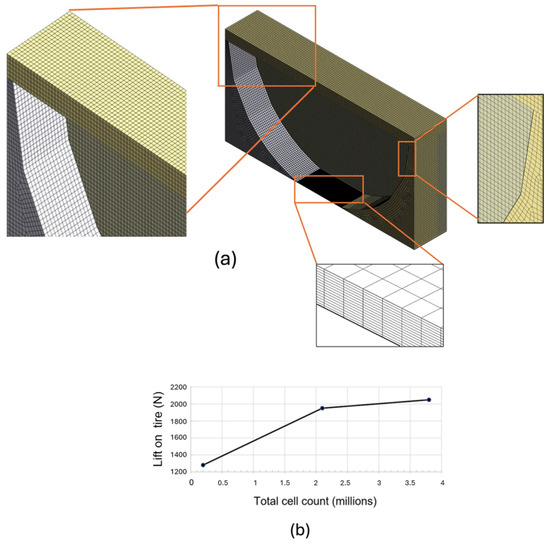
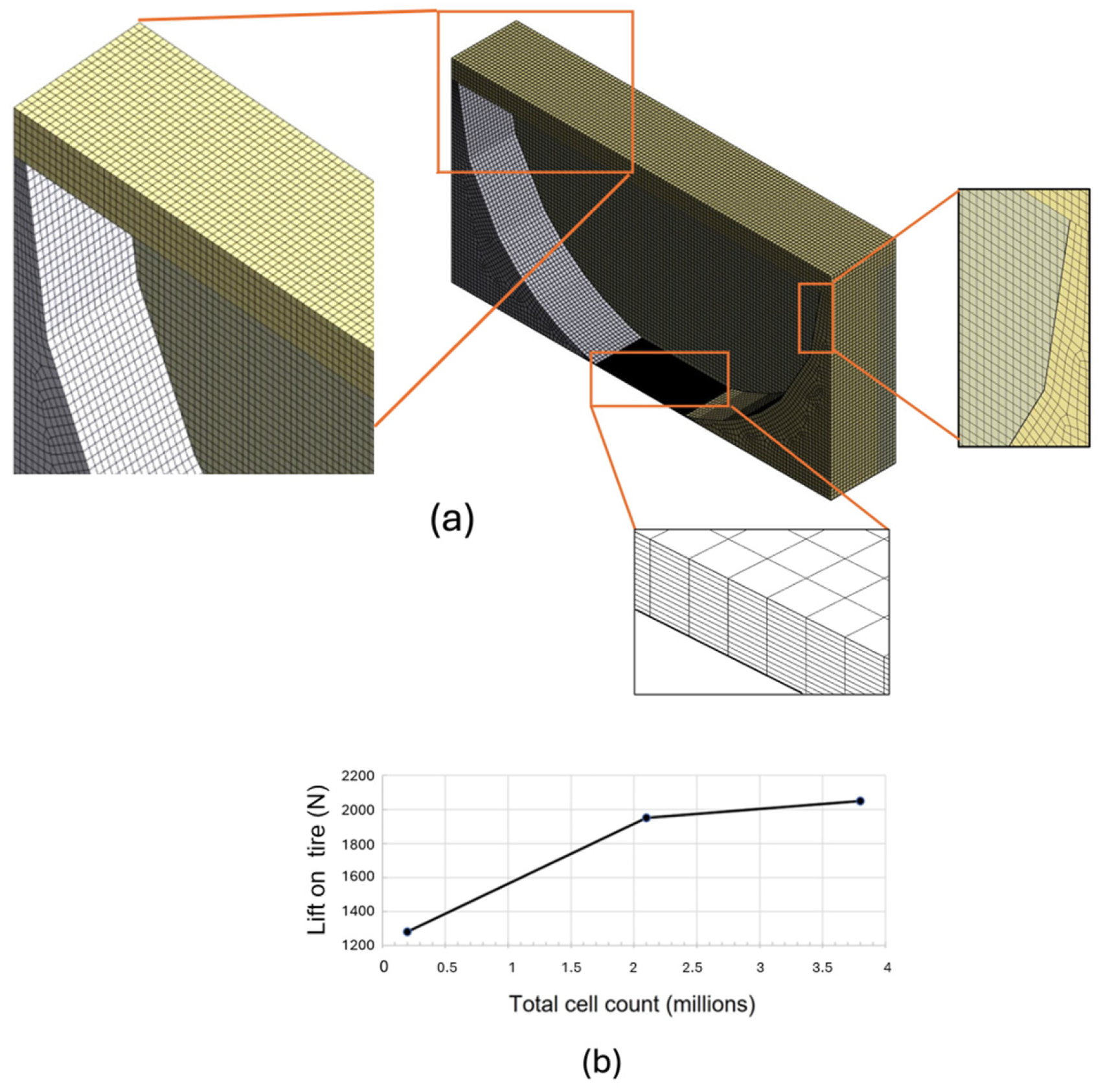
Three cases were examined, each with varying element counts to represent the gap height, under an inlet velocity of 60 km/h and a water film thickness of 7.62 mm. Care was taken to avoid high aspect ratio elements when altering the element count in the 0.5 mm gap beneath the tire. Figure 5b indicates that the calculated lift force on the tire asymptotes towards ~2100 N as the number of cells representing the gap between the tire patch and the pavement reaches 15 (corresponding to the mesh with 3.75 million cells overall and a tire–pavement contact patch of 0.035 m²). In this mesh, shown in Figure 5a, resolution in the 0.5 mm under-tire gap is 0.003 mm, resolution at the leading edge of the tire is ~0.5 mm, and resolution of the water film thickness and thus the air–water interface upstream of the tire is 1 mm.

Figure 5. (a) Computational domain and mesh for the tire–water–air configuration. The finest 3.75 million cell mesh (used for production runs) is shown. The mostly hexahedral mesh is shown with zoomed views highlighting the mesh in the leading edge of the tire (with resolution of ~0.5 mm) and in the thin water film region between the tire footprint and the pavement discretized by 15 cell layers (yielding a resolution of ~0.003 mm). The air–water interface upstream of the tire was meshed with resolution of ~1 mm. (b) Lift force on the tire as a function of cell (element) count.

3.2. Model Validation

Recall that all of the empirical equations against which the present CFD model is compared are derived directly from physical experiments: the NASA equation (Equation (1)) was developed from locked-wheel hydroplaning experiments conducted at the NASA Langley Research Center using aircraft and automobile tires on flooded smooth surfaces [2,3]; the TXDOT equation was derived from an extensive experimental program at Texas A&M University [4]; the PAVDRN equation is based on experimental data consolidated by the Pennsylvania Transportation Institute [5]; and the USF equation (Equation (2)) was calibrated against locked-wheel tester data for passenger vehicle tires [6]. The Ong and Fwa (2006) numerical model [7], also used for comparison, was itself validated against the NASA equation and its underlying experimental data. Thus, the comparisons presented in Figure 5 and Figure 6 are grounded in physically measured correlations rather than being model-to-model comparisons alone.

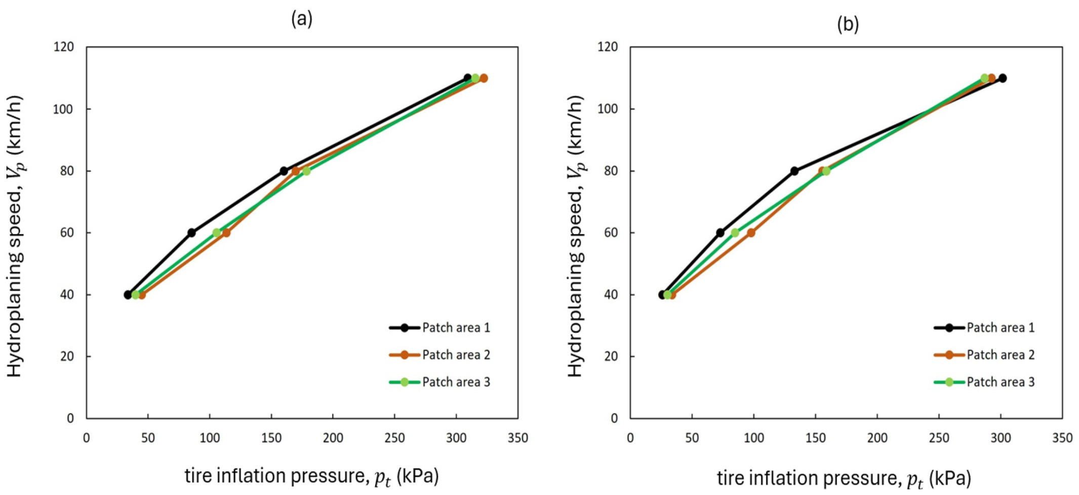
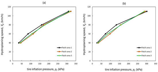
Figure 6. Solutions from the developed model using (a) k–ε (b) k–ω turbulence closures for three different patch areas of the tire geometry depicted in Figure 4.

The empirical NASA equation has been widely used in both numerical and experimental development of hydroplaning-related research work (e.g., [7,8,10,34]). Therefore, first, the developed CFD model was validated against Equation (1). To implement this, simulations were carried out with inlet flow/pavement velocities of 40, 60, 80, and 110 km h⁻¹, respectively, corresponding to the hydroplaning velocity.

Figure 6 shows the hydroplaning speeds (i.e., the inlet flow velocities) vs. the tire inflation pressure obtained from simulations using the k–ε model and k–ω model. The tire inflation pressures were calculated as described earlier in Section 2.5.1. The curves reported in Figure 6 were obtained with the developed model using three computational domains characterized by the three different bottom tire patch areas described earlier in Section 2.4.4. Patch areas 1, 2, and 3 are 0.03, 0.035, and 0.04 m², respectively. These three patch areas were shown to represent typical variations in the tire–pavement contact size under different tire loads and deflections. In all cases, the mesh resolution was controlled so that approximately 15 cells spanned the gap between the tire patch and the pavement, consistent with the mesh sensitivity analysis in Figure 5.

The hydroplaning speeds vs. the tire inflation pressure curves with the three patch areas are remarkably close to each other for each turbulence model. This behavior is expected from the NASA relation in Equation (1), which expresses the hydroplaning speed $V_p$ solely as a function of the inflation pressure $p_t$. In the relation $W=p_t{A}_{\mathrm{p}\mathrm{a}\mathrm{t}\mathrm{c}\mathrm{h}}$, a change in load $W$ is primarily accommodated by a change in the contact area $A_{\mathrm{p}\mathrm{a}\mathrm{t}\mathrm{c}\mathrm{h}}$, not by a change in $p_t$; therefore, when the results are plotted as $V_p$ versus $p_t$, moderate variations in $A_{\mathrm{p}\mathrm{a}\mathrm{t}\mathrm{c}\mathrm{h}}$ have little effect on the predicted curve.

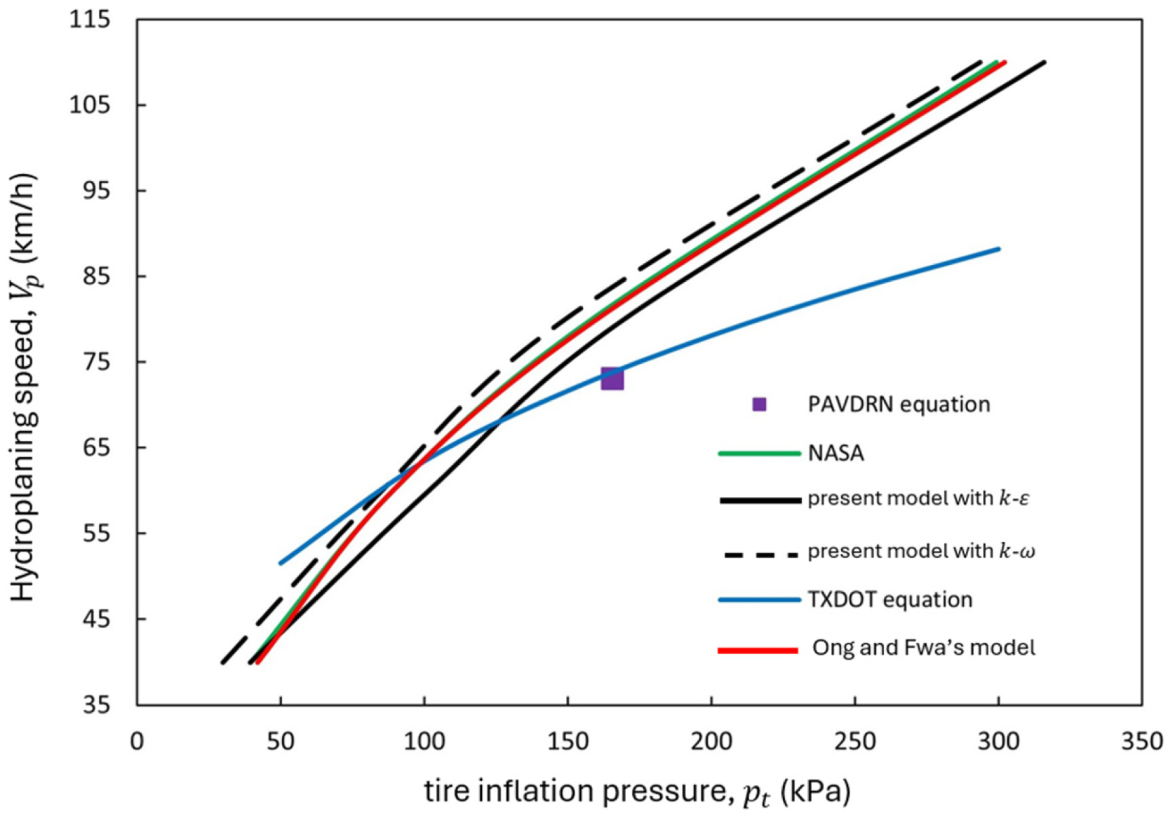
The results of Figure 6 for each turbulence model averaged over the three patch areas used are shown in Figure 7 along with the NASA empirical equation prediction, other empirical predictions and Ong and Fwa’s (2006) CFD model prediction [7]. These results from all models were obtained with a water film thickness or WFT of 7.62 mm upstream of the tire. The hydroplaning speeds exhibited by the CFD simulations with the k–ε and k–ω turbulence models are in good agreement with both the NASA equation and Ong and Fwa’s (2006) model. The present model with the k–ε closure results in a maximum of 6% underprediction of the hydroplaning speed vs. tire inflation pressure, while the k–ω model performs better at a maximum of 2.4% overprediction, relative to the NASA equation. Further discussion regarding the difference in these results between the k–ε and k–ω models is given in Section 3.4. The PAVDRN and TXDOT equations predict the same hydroplaning speeds for WFT greater than 2.4 mm (as seen in both Figure 7 and Figure 8) because of their common basis. The TXDOT equation does not fall along the line of the NASA hydroplaning equation due to the conservative constants that the former uses.

Figure 7. Comparison in terms of $V_p$ vs. $p_t$ of averaged solutions from the present model with the $\mathrm{k}$–ε and $\mathrm{k}-\mathsf{\omega }$ turbulence closures with empirical models and Ong and Fwa’s (2006) [7] numerical model.

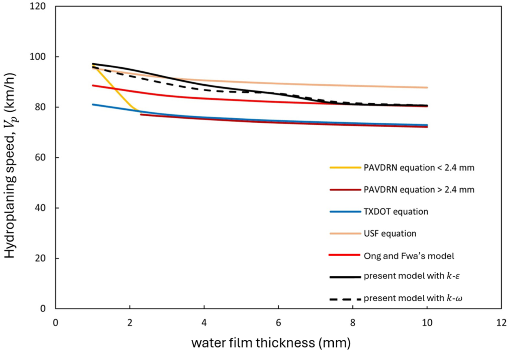
Figure 8. Comparison in terms of $V_p$ vs. $\mathrm{W}\mathrm{F}\mathrm{T}$ of averaged solutions from the present model with the k–ε and k–$\omega$ turbulence closures with empirical models and Ong and Fwa’s (2006) [7] model.

It should be mentioned that the geometric representation of Ong and Fwa’s (2006) model [7] did not include the tire’s leading edge and only considered the tire’s footprint. This geometric simplification thus prevented their model from capturing the flow stagnation that occurs at the leading edge of the tire. The accuracy of the Ong and Fwa model seen in Figure 7, despite this key omission, suggests that accurate hydroplaning prediction does not require embedding the correct tire shape. However, surely the lift on the bottom of the tire in Ong and Fwa’s model is likely greater than in a more realistic representation of a tire that includes the leading edge, such as the present model.

Figure 8 shows the variation of the hydroplaning speed with WFT. These results from all models were obtained for a fixed tire inflation pressure of 165.5 kPa. Recall Section 2.5.1 for the description of the solution strategy followed in obtaining these results with the present model. The prediction of the present model with both turbulence closures again is in good agreement with Ong and Fwa’s (2006) model [7], especially for WFT > 8 mm. Furthermore, the present model predictions are in good agreement with the USF equation for WFT < 4 mm.

3.3. Characterization of the Turbulence in the Vicinity of the Tire

In this section, a characterization of the flow in the vicinity of the tire is presented using the simulation performed with WFT = 7.2 mm, $A_{patch}=0.3$ m², inlet/pavement velocity $U=110$ km h⁻¹ and the k–$\omega$ model.

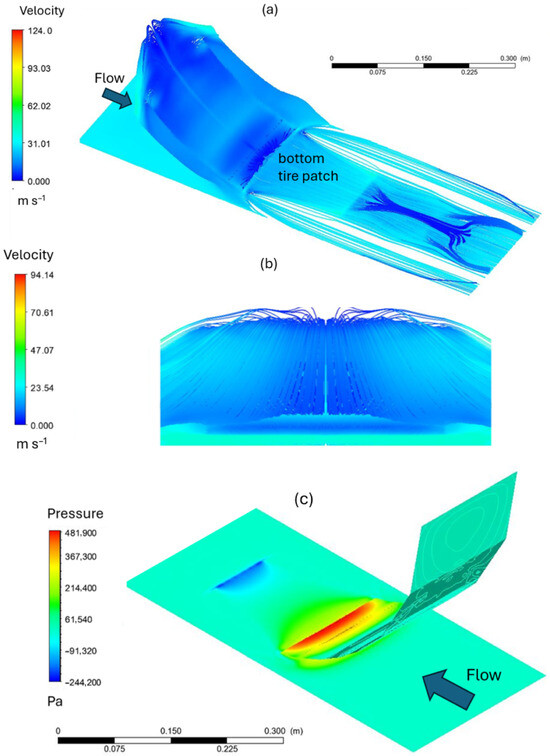
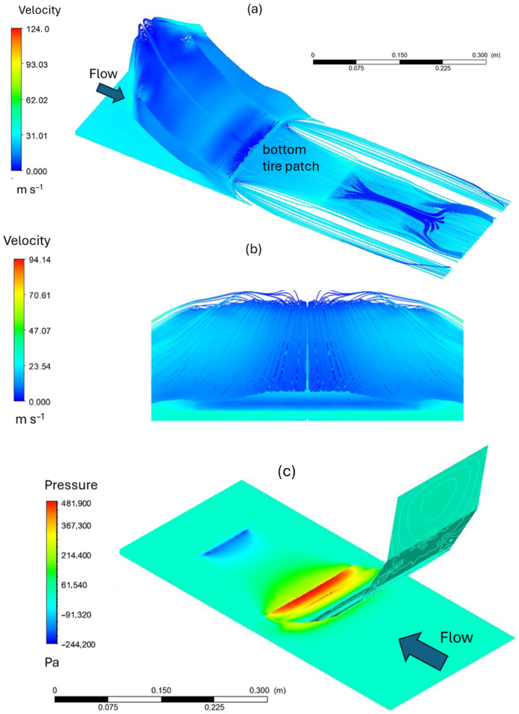
Figure 9a,b shows the velocity contours and velocity streamlines around and under the tire below the bottom tire rectangular patch and the resulting water pileup at the front of the tire. A portion of the incoming water stagnates ahead of the tire, while the majority is diverted laterally around the sides and through the thin under-tire gap.

Figure 9. Flow structure and pressure distribution around the smooth tire during hydroplaning. (a) Three-dimensional streamline visualization illustrating water stagnation at the lower leading edge (characterized by near zero velocity) and redistribution below the bottom tire patch. (b) Front view (in the direction of flow into page) demonstrating a bow-wave formation and vertical flow redistribution associated with water stagnation at the lower leading edge of the tire. (c) Pressure contours indicating localized high pressures in the lower leading edge stagnation region towards the bottom of the tire, which dominates the hydrodynamic lift.

A volumetric balance indicates that approximately 99.4% of the inflowing water exits around the sides of the domain, with only a small fraction (0.6%) exiting through the far end outlet (recall Figure 4). This strong lateral diversion is hydraulically significant, limiting the stagnation pressure that can develop at the leading edge of the tire and the pressure underneath the tire, thereby influencing the hydroplaning speed.

The associated pressure field is shown in Figure 9c, where high pressures are localized at the leading edge towards the bottom of the tire. Taking a representative peak pressure of about 500 kPa and an effective modulus for a stiffened vehicle tire in the range 500–1000 MPa, the corresponding normal strain is, at most, $\sim p/E\lesssim 5\times {10}^{-4}$–${10}^{-3}$. Such small strains indicate that the tire deformation is too weak to significantly alter the hydrodynamic pressure distribution. This supports the use of the decoupled tire–water model adopted here, in which dynamic tire deformation is neglected and the tire is treated as rigid.

The high-pressure levels observed along the leading edge of the tire indicate a stagnation-type flow behavior consistent with classical stagnation scaling. For the representative case shown in Figure 9c, the peak pressure difference at the tire front is approximately $p-p_{\mathrm{\infty }}\approx 4.82\times {10}^5\hspace{0.17em}\mathrm{P}\mathrm{a}$. Calculating the corresponding dynamic pressure based on the approach velocity $U=110\mathrm{k}\mathrm{m}{\mathrm{h}}^{-1}$ and water density $\rho =998.2\mathrm{k}\mathrm{g}{\mathrm{m}}^{-3}$ results in a stagnation pressure coefficient $C_p=(p-p_{\mathrm{\infty }})/\left(0.5\rho U^2\right)=1.03\approx 1$. A value of $C_p$ in close unity is characteristic of stagnation-point flow in which the incoming momentum is efficiently converted into pressure, as expected for an impingement-type configuration. Furthermore, this near-unity pressure coefficient provides a useful consistency check indicating that the leading-edge pressure buildup follows classical stagnation scaling.

Consistent with this pressure buildup, surfaces along the leading edge towards the bottom of the tire (see surfaces S6 and S7 in Figure 4) bear the highest percentage of the lift, as listed in Table 2. The pressure underneath the tire (on the bottom tire patch (surface S8)) also bears a significant portion of the lift. The upper leading-edge surfaces (S1, S2, S3, and S4) along the splash zone (recall Figure 2) carry minimal lift.

Table 2. Lift carried by each planar surface (surfaces S1–S8) used to represent the tire geometry, as labeled in Figure 4.

Surface Name	Lift on the Surface	Percentage of the Total Lift (%)
Surface 1 (S1)	8.9	0.3
Surface 2 (S2)	119.4	4.7
Surface 3 (S3)	42.7	1.7
Surface 4 (S4)	81.8	3.2
Surface 5 (S5)	192.7	7.5
Surface 6 (S6)	791.3	31.0
Surface 7 (S7)	586.3	23.0
Surface 8 (S8) (bottom tire patch)	730.4	28.6
Total lift on the tire	2553.5	100

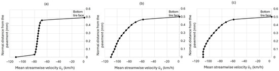
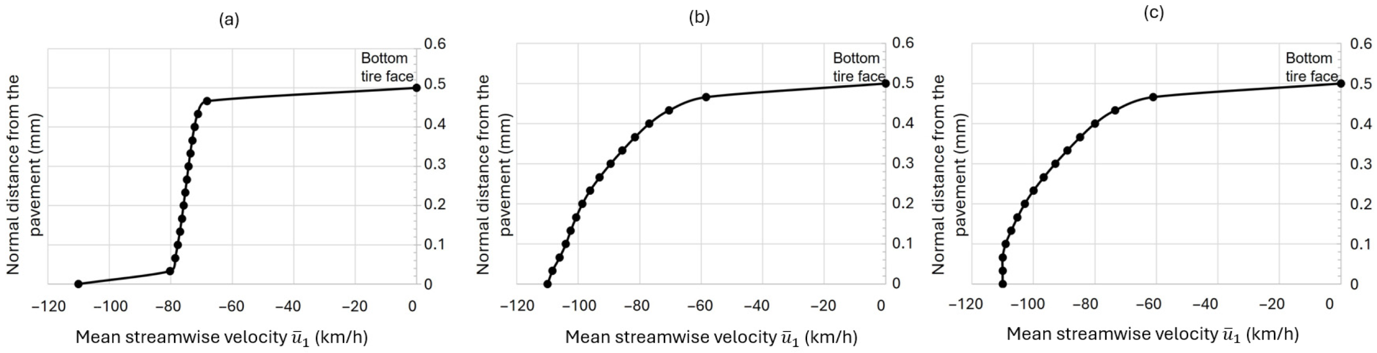
The fluid velocity profiles underneath the bottom tire patch are shown in Figure 10. In all profiles, the flow velocity matches the velocity of the stationary tire and the moving pavement, set through the boundary conditions. Towards the front, underneath the bottom tire patch (Figure 10a), the bulk flow moves at ~80 km h⁻¹, slower than the pavement velocity of 110 km h⁻¹, likely due to the water film’s sudden encounter with the tire. Further downstream, towards the middle and back, underneath the bottom tire patch, the bulk flow recovers momentum, as the fluid close to the pavement flows at roughly the same speed as the pavement, as expected from the no-slip condition at the pavement.

Figure 10. Flow velocity profiles underneath the (a) front, (b) middle, and (c) back of the tire patch (face) for an inlet flow and pavement velocity of 110 km h⁻¹.

In all velocity profiles in Figure 10, the high shear in the velocity at the bottom face of the stationary tire gives rise to shear-dominated turbulence. Recall our model simplification, depicted in Figure 2, which imposes a uniform gap between the bottom of the tire and the pavement instead of prescribing the actual deformed tire footprint, as measured in physical experiments during hydroplaning. By ensuring a uniform 0.5-mm gap beneath the tire, the turbulence in the flow through this gap can be straightforwardly characterized to be of the shear-dominated type that exists in the pressure-gradient driven flow between two no-slip flat surfaces, a canonical turbulence regime well-investigated in the literature [42]. The friction Reynolds number in this classical flow is defined as follows:

$$R{e}_{\tau }={\displaystyle \frac{u_{\tau }h}{\nu }}$$

(22)

where $h$ is the channel height, $u_{\tau }$ is the friction velocity, and $\nu$ is kinematic viscosity [42]. For water, $\nu$ = 10⁻⁶ m² s⁻¹, and for the 0.5-mm gap between the bottom tire patch and the pavement in our model, $h$ = 0.5 mm. Furthermore, the friction velocity can be defined as follows:

$$u_{\tau }=\sqrt{{\displaystyle \frac{{\tau }_{\mathrm{t}\mathrm{i}\mathrm{r}\mathrm{e}}}{\rho }}}$$

(23)

where, for water, the density is $\rho =$ 998.2 kg/m³, and the viscous shear stress between the water film and the bottom tire patch is defined using Newton’s Law of Viscosity:

$${\tau }_{\mathrm{t}\mathrm{i}\mathrm{r}\mathrm{e}}=\mu {\left({\displaystyle \frac{d{\overline{u}}_1}{dy}}\right)}_{\begin{array}{c}\mathrm{a}\mathrm{t}\mathrm{b}\mathrm{o}\mathrm{t}\mathrm{t}\mathrm{o}\mathrm{m}\\ \mathrm{t}\mathrm{i}\mathrm{r}\mathrm{e}\mathrm{p}\mathrm{a}\mathrm{t}\mathrm{c}\mathrm{h}\end{array}}$$

(24)

where the dynamic viscosity for water is 0.001 Pa$\cdot$s. From Figure 10, the shear rate can be measured as ${\left(d{\overline{u}}_1/dy\right)}_{\mathrm{a}\mathrm{t}\mathrm{b}\mathrm{o}\mathrm{t}\mathrm{t}\mathrm{o}\mathrm{m}\mathrm{t}\mathrm{i}\mathrm{r}\mathrm{e}\mathrm{p}\mathrm{a}\mathrm{t}\mathrm{c}\mathrm{h}}$ = 5.54 × 10⁵ s⁻¹, 5.19 × 10⁵ s⁻¹, and 5.23 × 10⁵ s⁻¹ towards the front, the middle, and back of the bottom tire patch, respectively. Based on these three values of the shear rate, the friction Reynolds numbers are $R{e}_{\tau }$ = 370, 360, and 360, respectively. These values place the under-tire flow within the regime of wall-bounded turbulent shear [42].

As noted earlier in Section 2.2, the realizable k–ε model was solved with standard wall functions, whereas the SST k–ω model was solved with Fluent’s correlation-based near-wall treatment, which is a y+ insensitive formulation. For the hydroplaning case previously analyzed, the wall-normal distance from the first-cell-center to the bottom tire patch (i.e., the wall), $y_1$ in wall or plus units is $y_1^{+}$ ≈ 12, following the definition $y_1^{+}=y_1{u}_{\tau }/\nu .$ The value of $y_1^{+}=12$ indicates an intermediate y+ treatment in the under-tire gap rather than full viscous-sublayer resolution. The mesh strategy was objective-based: refinement was concentrated in the 0.5 mm under-tire gap (the principal shear-dominated region governing pressure buildup and lift) (as described earlier in Section 3.1) and adequacy was assessed through convergence of the integrated lift and the captured stagnation pressure coefficient on the leading edge of the tire of $C_p$ ≈ 1, rather than through local viscous-sublayer resolution everywhere on the tire surface.

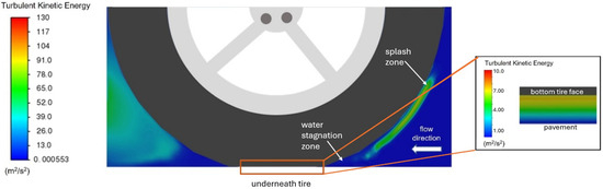
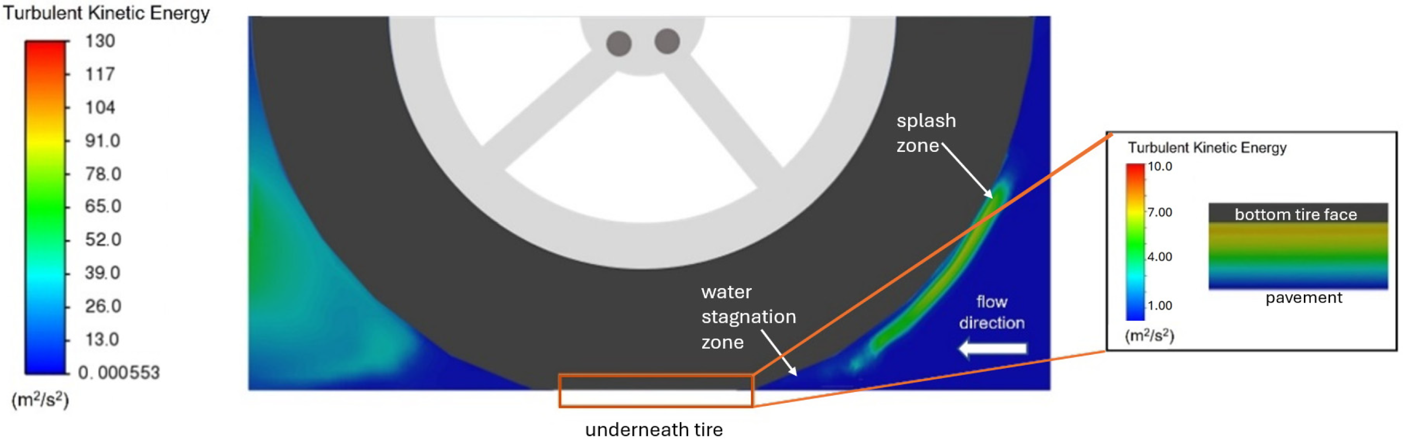
Figure 11 shows contours of TKE around the tire. The TKE levels are negligible upstream of the tire because the air, water, and pavement move at the same speed (recall Figure 3), resulting in negligible shear and thus negligible production of TKE. Elevated TKE values are observed in the thin water sheet or splash zone (sketched in Figure 2) that accelerates upward along the front curvature of the tire following the stagnation region. This zone is characterized by strong velocity gradients and interfacial shear between the rapidly accelerating water layer and the surrounding air, leading to enhanced production of TKE through the mean shear production term in the turbulence model.

Figure 11. TKE around the tire on the plane located at the middle of the spanwise length of the domain.

In the splash zone, the TKE reaches peak values of $k\approx 90$ m²/s². This corresponds to root mean square velocity fluctuations of $u_{\mathrm{r}\mathrm{m}\mathrm{s}}^{\prime }\approx \sqrt{2k/3}\approx 7.7\mathrm{m}$/s. For a representative hydroplaning speed of $U\approx 30.6$ m/s (110 km/h), the local turbulence intensity is therefore $I=u_{\mathrm{r}\mathrm{m}\mathrm{s}}^{\prime }/U\approx 0.25$, i.e., about 25%, and thus significant relative to the bulk flow.

Note that the splash zone does not contribute significantly to the lift on the tire, as pressures there are small compared to the stagnation zone in the lower leading edge of the tire (Figure 9c). By contrast, the stagnation zone exhibits comparatively low TKE levels. This behavior is consistent with stagnation-point flow physics: although pressure is maximized in this region, the local velocity magnitude and associated shear are small, resulting in modest turbulence production.

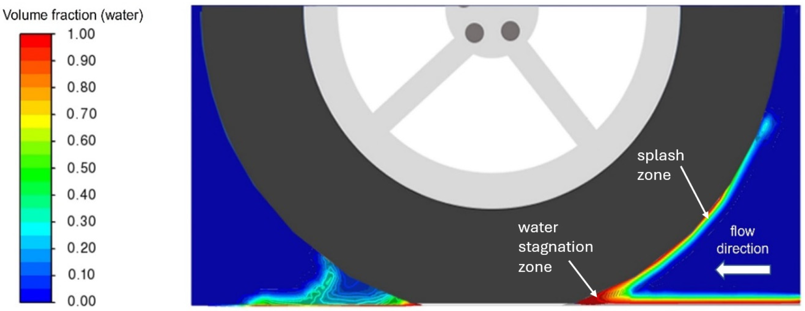
The distinction between these water stagnation and splash zones is further evident in the volume fraction contours shown in Figure 12. The stagnation zone corresponds to water accumulation near the pavement, while the splash region corresponds to the thin, accelerating water sheet that forms downstream of stagnation.

Figure 12. Volume fractions of water and air around the tire on the plane located at the middle of the spanwise length of the domain. Volume fraction showing water occupying the gap underneath the tire (between the tire and the pavement) is not visible.

The Figure 11 inset shows the TKE distribution underneath the tire in the 0.5 mm gap between the tire and the pavement, characterized by elevated values near the bottom face of the tire relative to the pavement. The high velocity shear near the bottom face of the tire observed in Figure 10 is responsible for the elevated values of TKE in this region.

Finally, Figure 11 also reveals a zone of high TKE behind the tire associated with turbulence in the airside of the flow. Note that these airside dynamics do not contribute to the lift on the tire, thus they are outside of the scope of the present study.

3.4. Effect of Turbulence Modeling on Hydroplaning Speed

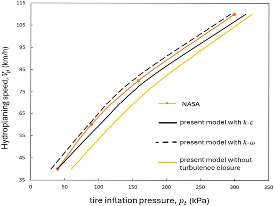
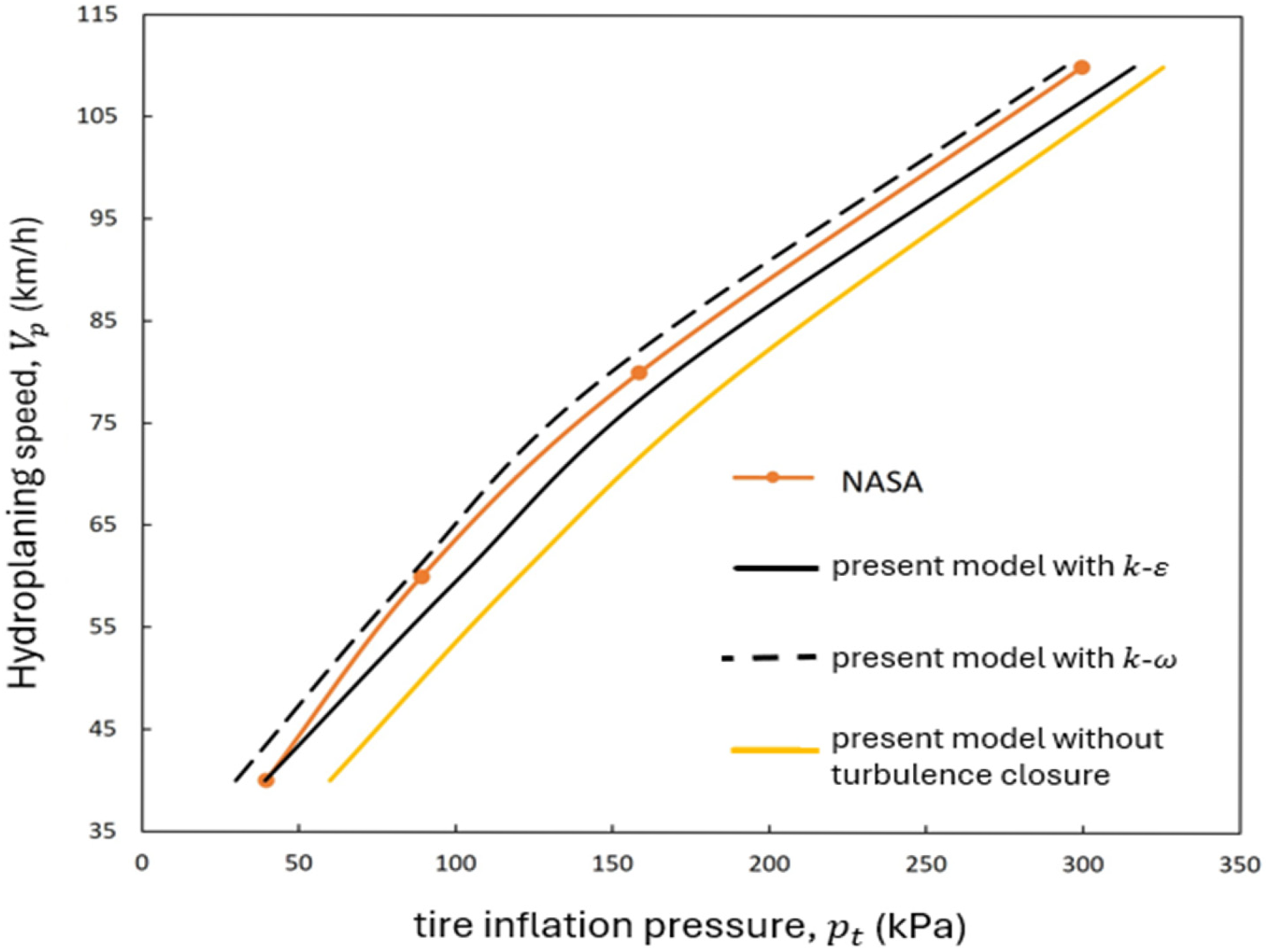
Figure 13 presents $V_p$ vs. $p_t$ obtained with and without turbulence modeling. The laminar formulation (i.e., CFD without turbulence modeling) underpredicts the hydroplaning speeds by approximately 13.5% on average relative to the NASA equation and also underpredicts the speeds obtained with the turbulence closures. In the laminar equations (Equations (3) and (4)), no turbulent shear stresses appear in the momentum balance. Consequently, no turbulence-induced redistribution or dissipation mechanisms are represented in the mean flow, and the computed pressure field yields a larger integrated hydrodynamic lift for a given inlet/pavement velocity. A lower speed is therefore sufficient to balance the wheel load in the laminar simulations.

Figure 13. Comparison in terms of $V_p$ vs. $p_t$ of averaged solutions from the present model with the k–ε and k–$\omega$ turbulence closures, the present model without turbulence closure (laminar solution) and the NASA hydroplaning empirical equation.

However, turbulence is generated immediately downstream of stagnation in the splash region and within the thin under-tire gap. As shown earlier, the under-tire flow can reach friction Reynolds numbers $R{e}_{\tau }\approx 360–370$, placing it firmly within the regime of wall-bounded turbulent shear flow. In this regime, the Reynolds stresses contribute significantly to the momentum balance (see Equation (8)) and enhance the shear-driven momentum redistribution within the confined gap.

From a mechanical-energy perspective, the inclusion of turbulence closure introduces additional effective shear stresses that act analogously to distributed hydraulic resistance. These stresses increase mixing and dissipation within the under-tire and splash regions. Although the approach flow upstream of the tire exhibits negligible turbulence production, the turbulence generated locally in the shear-dominated under-tire and splash regions modifies the overall pressure distribution by reducing the mean mechanical energy available for conversion into sustained static pressure lifting the tire.

As a result, even though the stagnation mechanism remains efficient, the integrated hydrodynamic lift for a given speed is reduced relative to the laminar case. A higher inlet/pavement velocity is therefore required to achieve the lift–load balance corresponding to hydroplaning, explaining the upward shift of the turbulence-model curves toward the NASA relation observed in Figure 13.

Finally, note that the differences between the SST k–$\omega$ and realizable k–$\epsilon$ closures lead to modest variations in the predicted stagnation pressure and lift, consistent with the known behavior of these models in stagnation-dominated flows [43,44]. However, these second-order differences do not alter the primary conclusion: neglecting turbulence introduces a systematic bias in the hydroplaning speed prediction by overestimating the recoverable pressure field beneath the tire. Nevertheless, it would be interesting to explore these differences in the future via comparisons against the LES or DNS.

4. Summary and Conclusions

This study examined the role of turbulence modeling in CFD-based prediction of vehicle hydroplaning speed using a three-dimensional RANS–VoF model of a smooth tire sliding in locked-wheel mode over flooded, nominally smooth pavement. The tire was represented as a rigid body with an idealized rectangular footprint whose area was linked to tire load and inflation pressure, allowing the hydrodynamic response to be separated from uncertainties in tire deformation.

Steady-state hydroplaning was simulated over a 7.62 mm water film with a 0.5 mm gap between the tire and the pavement, for inflation pressures between 100 and 300 kPa, and the resulting hydroplaning speeds were compared with the NASA hydroplaning equation and other empirical and numerical models. Recalling objectives (1) and (2) of this study given in the Introduction, for the hydroplaning-speed–versus–inflation-pressure relationship, the model without turbulence closure (laminar formulation) leads to a consistent, systematic underprediction of the hydroplaning speeds by about 13.5% on average relative to the NASA equation. Including turbulence via the realizable k–ε or SST k–ω closure removes this bias, significantly improving agreement: the k–ε model yields a maximum underprediction of about 6%, while the k–ω model slightly overpredicts the hydroplaning speeds by, at most, 2.4%. Similar agreement is obtained for the hydroplaning-speed–versus–water-film-thickness curve at a fixed inflation pressure of 165.5 kPa, where the present model closely follows both the Ong and Fwa (2006) [7] numerical model and the USF equation over most of the water film range considered. These results demonstrate that explicitly accounting for turbulence in the tire vicinity is essential for reproducing empirical hydroplaning trends and for avoiding overly conservative estimates based on the laminar flow assumption made in a significant number of hydroplaning modeling studies throughout the published literature (Table 1).

The simulations also clarify how turbulence manifests in the flow field beneath and in front of the tire. Recalling objective (3), under the rectangular tire footprint, the velocity profiles in the 0.5 mm gap indicate a shear-dominated, turbulent regime reaching friction Reynolds numbers $\mathrm{R}{\mathrm{e}}_{\mathsf{\tau }}\approx 360-370$. At the front of the tire, the TKE peaks at $\mathrm{k}\approx 90$ m²/s², corresponding to a local turbulence intensity of about 25% (relative to the inlet airflow speed) and characterizing a strongly turbulent water jet running upward along the tire away from the stagnation zone. Compared with the laminar computation at the same external speed, the inclusion of turbulence introduces additional mixing and energy dissipation in these regions. Consequently, the integrated hydrodynamic lift for a given speed is smaller than in the laminar solution, and a higher speed is required to achieve the lift–load balance needed for hydroplaning.

Regarding objective (4), by comparing three realistic footprint areas (0.03, 0.035, and 0.04 m²), corresponding to per-tire loads of approximately 1.5–12 kN, this study also shows that the predicted hydroplaning-speed–versus–pressure curves are relatively insensitive to moderate variations in the bottom tire patch area when the results are plotted against inflation pressure, consistent with the structure of the NASA empirical equation. Finally, an order-of-magnitude estimate of tire strain under the peak hydrodynamic pressures ($\sim 500\mathrm{k}\mathrm{P}\mathrm{a}$) indicates deformations (strains) well below ${10}^{-3}$, supporting the use of a rigid tire representation for the smooth-tire, smooth-pavement conditions considered here.

The present work emphasizes that turbulence in both the under-tire shear layer and the front splash region is hydraulically significant and must be represented in CFD models intended for hydroplaning risk assessment. At the same time, the simplified rigid-tire, smooth-pavement configuration and steady RANS framework omit several important effects, including tire tread geometry, pavement macrotexture, transient braking, or rolling conditions, and the fine-scale turbulent structures in the splash and gap regions. Future work should therefore extend the approach to perhaps computationally feasible zonal LES approaches coupled with fluid–structure interaction while using RANS as guidance for parameter ranges and initial conditions. The zonal LES methodology would adapt the mesh and eddy viscosity so as to behave like LES in the under-tire and leading edge splash regions while reverting to the RANS approach in other regions. Such developments would further improve the mechanistic understanding of tire–water–pavement interaction and support more refined criteria for highway drainage design, tire tread design, and hydroplaning mitigation.

References

- Dehnad, M.H.; Yazdi, A. A review of numerical and experimental studies on hydroplaning of vehicles in motion on road surfaces. Results Eng. 2024, 23, 102438. [Google Scholar] [CrossRef] [Scilit]
- Horne, W.B.; Joyner, U.T. Pneumatic tire hydroplaning and some effects on vehicle performance. SAE Trans. 1966, 74, 623–650. [Google Scholar]
- Horne, W.B.; Ivey, D.L.; Yager, T.J. Recent studies to investigate effects of tire footprint aspect ratio on dynamic hydroplaning speed. In Tire Science and Technology; ASTM International: West Conshohocken, PA, USA, 1986; pp. 26–46. [Google Scholar]
- Gallaway, B.M.; Ivey, D.L.; Hayes, G.; Ledbetter, W.B.; Olson, R.M.; Woods, D.L.; Schiller, R.F., Jr. Pavement and Geometric Design Criteria for Minimizing Hydroplaning; Technical Report No. FHWA-RD-79-31; Federal Highway Administration (FHWA): Washington, DC, USA, 1979. [Google Scholar]
- Huebner, R.S.; Anderson, D.A.; Warner, J.C.; Reed, J.R. PAVDRN: Computer model for predicting water film thickness and potential for hydroplaning on new and reconditioned pavements. Transp. Res. Rec. 1997, 1599, 128–131. [Google Scholar] [CrossRef] [Scilit]
- Gunaratne, M.; Lu, Q.; Yang, J.; Metz, J.; Jayasooriya, W.; Yassin, M.; Amarasiri, S. Hydroplaning on Multi Lane Facilities; Technical Report No. BDK84 977-14; Florida Department of Transportation: Tallahassee, FL, USA, 2012.
- Ong, G.P.; Fwa, T.F. Transverse pavement grooving against hydroplaning. I: Simulation model. J. Transp. Eng. 2006, 132, 441–448. [Google Scholar] [CrossRef] [Scilit]
- Ong, G.P.; Fwa, T.F. Wet-pavement hydroplaning risk and skid resistance: Modeling. J. Transp. Eng. 2007, 133, 590–598. [Google Scholar] [CrossRef] [Scilit]
- Nazari, A.; Chen, L.; Battaglia, F.; Ferris, J.B.; Flintsch, G.; Taheri, S. Prediction of hydroplaning potential using fully coupled finite element–computational fluid dynamics tire models. J. Fluids Eng. 2020, 142, 101202. [Google Scholar] [CrossRef] [Scilit]
- Deng, T.; Wang, S.; Cheng, D.; Zheng, L.; Ren, L. Effects of driving conditions on tire hydroplaning performance. Lubricants 2025, 13, 76. [Google Scholar] [CrossRef] [Scilit]
- Ding, Y.; Wang, H. Evaluation of hydroplaning risk on permeable friction course using tire–water–pavement interaction model. Transp. Res. Rec. 2018, 2672, 408–417. [Google Scholar] [CrossRef] [Scilit]
- Liu, X.; Cao, Q.; Wang, H.; Chen, J.; Huang, X. Evaluation of vehicle braking performance on wet pavement surface using an integrated tire–vehicle modeling approach. Transp. Res. Rec. 2019, 2673, 295–307. [Google Scholar] [CrossRef] [Scilit]
- Löwer, J.; Wagner, P.; Unrau, H.-J.; Bederna, C.; Gauterin, F. Physical model of tire–road contact under wet conditions. Tribol. Lett. 2020, 68, 25. [Google Scholar] [CrossRef] [Scilit]
- Tao, S.; Wang, J.; Dong, R. Model construction and numerical simulation for hydroplaning of complex tread tires. Complex Syst. Model. Simul. 2022, 2, 322–333. [Google Scholar] [CrossRef] [Scilit]
- Zhou, C.; Zhong, Q.; He, Z.; Wang, Y.; Tang, X.; Li, P. Analysis of tire–pavement viscous hydroplaning based on the material point method. Phys. Fluids 2025, 37, 083121. [Google Scholar] [CrossRef] [Scilit]
- Zhu, S.; Liu, X.; Cao, Q.; Huang, X. Numerical study of tire hydroplaning based on power spectrum of asphalt pavement and kinetic friction coefficient. Adv. Mater. Sci. Eng. 2017, 2017, 5843061. [Google Scholar] [CrossRef] [Scilit]
- Kim, T.-W.; Jeong, H.-Y. Hydroplaning simulations for tires using FEM, FVM and an asymptotic method. Int. J. Automot. Technol. 2010, 11, 901–908. [Google Scholar] [CrossRef] [Scilit]
- Schulz, H.E.; Curry, J.E.; Simões, A.L.A. Water films and hydroplaning on highways: Hydrodynamic aspects. J. Transp. Eng. B Pavements 2021, 147, 04021053. [Google Scholar] [CrossRef] [Scilit]
- Zheng, B.; Huang, X.; Zhang, W.; Zhao, R.; Zhu, S. Adhesion characteristics of tire–asphalt pavement interface based on a proposed tire hydroplaning model. Adv. Mater. Sci. Eng. 2018, 2018, 5916180. [Google Scholar] [CrossRef] [Scilit]
- El-Sayegh, Z.; El-Gindy, M. Sensitivity analysis of truck tire hydroplaning speed using FEM–SPH model. Int. J. Veh. Syst. Model. Test. 2017, 12, 143–161. [Google Scholar]
- Hermange, C.; Oger, G.; Le Chenadec, Y.; Le Touzé, D. A 3D SPH–FE coupling for FSI problems and its application to tire hydroplaning simulations on rough ground. Comput. Methods Appl. Mech. Eng. 2019, 355, 558–590. [Google Scholar] [CrossRef] [Scilit]
- Cai, J.; Du, N.; Zhou, N.; Li, Y.; Dai, X.; Zhang, H. Numerical study of the tire hydroplaning behavior of aircraft on grooved concrete pavement. PLoS ONE 2023, 18, e0292701. [Google Scholar] [CrossRef] [Scilit] [PubMed]
- Chen, X.; Wang, H. Analysis and mitigation of hydroplaning risk considering spatial–temporal water condition on the pavement surface. Int. J. Pavement Eng. 2023, 24, 2036988. [Google Scholar] [CrossRef] [Scilit]
- Chen, G.; Liu, H.; Gao, Y.; Ma, Q.; Pan, F.; Liu, C. Simulation analysis of tire hydroplaning performance based on CFD. Int. J. Appl. Sci. Math. 2022, 9, 78–87. [Google Scholar]
- Cho, J.R.; Lee, H.W.; Sohn, J.S.; Kim, G.J.; Woo, J.S. Numerical investigation of hydroplaning characteristics of three-dimensional patterned tire. Eur. J. Mech.—A/Solids 2006, 25, 914–926. [Google Scholar] [CrossRef] [Scilit]
- Zhou, H.C.; Wang, G.L.; Yang, J.; Xue, K.X. Numerical simulation of tire hydroplaning and its influencing factors. Appl. Mech. Mater. 2014, 602, 580–585. [Google Scholar] [CrossRef] [Scilit]
- Zhou, H.C.; Wang, G.L.; Yang, J.; Xue, K.X. Numerical simulation of effect of bionic V-riblet non-smooth surface on tire anti-hydroplaning. J. Cent. South Univ. 2015, 22, 3900–3908. [Google Scholar] [CrossRef] [Scilit]
- Aboelsaoud, M.; Elgamal, H.; Taha, A.A.; Abo Elazm, M. Comparative analysis of hydroplaning in electric and ICE vehicles. In Proceedings of the 2022 IEEE 2nd International Maghreb Meeting of the Conference on Sciences and Techniques of Automatic Control and Computer Engineering (MI-STA), Sabratha, Libya, 23–25 May 2022. [Google Scholar]
- Zeng, W.; Wu, W.; Li, Z.; Chen, W.; Gao, J.; Fu, B. A simulation of tire hydroplaning based on laser scanning of road surfaces. Appl. Sci. 2025, 15, 5577. [Google Scholar] [CrossRef] [Scilit]
- Cabut, D.; Michard, M.; Simoens, S.; Mees, L.; Todoroff, V.; Hermange, C.; Le Chenadec, Y. Analysis of the water flow inside tire grooves of a rolling car using refraction particle image velocimetry. Phys. Fluids 2021, 33, 032101. [Google Scholar] [CrossRef] [Scilit]
- Hermange, C.; Todoroff, V.; Biesse, F.; Le-Chenadec, Y. Experimental investigation of the leading parameters influencing the hydroplaning phenomenon. Veh. Syst. Dyn. 2022, 60, 2375–2392. [Google Scholar] [CrossRef] [Scilit]
- Vilsan, A.; Sandu, C.; Anghelache, G.; Warfford, J. Methodology for real-time hydroplaning risk estimation using an intelligent tire system: An analytical approach. Sensors 2025, 25, 7299. [Google Scholar] [CrossRef] [Scilit]
- Jeong, J.Y.; Jeong, H.Y. Hydroplaning simulation of a tire in thin water using FEM and an estimation method and its application to skid number estimation. Int. J. Automot. Technol. 2013, 14, 325–331. [Google Scholar] [CrossRef] [Scilit]
- Ong, G.P. Hydroplaning and Skid Resistance Analysis Using Numerical Modeling. Ph.D. Thesis, National University of Singapore, Singapore, 2006. [Google Scholar]
- Batchelor, G.K. An Introduction to Fluid Dynamics; Cambridge University Press: Cambridge, UK, 1967. [Google Scholar]
- ANSYS Inc. Fluent Theory Guide; ANSYS Inc.: Canonsburg, PA, USA, 2019. [Google Scholar]
- ANSYS Inc. Fluent User’s Guide; ANSYS Inc.: Canonsburg, PA, USA, 2019. [Google Scholar]
- Wilcox, D.C. Turbulence Modeling for CFD; DCW Industries: La Cañada, CA, USA, 1998. [Google Scholar]
- FHWAInfo Technology, U.S. Department of Transportation. Pavements—Locked-Wheel Tester (LWT). Available online: https://infotechnology.fhwa.dot.gov/locked-wheel-tester/ (accessed on 8 July 2024).
- National Academies of Sciences, Engineering, and Medicine. Guide for Pavement Friction; National Academies of Sciences, Engineering, and Medicine: Washington, DC, USA, 2009. [Google Scholar]
- Kelecy, F.J. Coupling momentum and continuity increases CFD robustness. ANSYS Advant. 2008, 2, 49–51. [Google Scholar]
- Pope, S.B. Turbulent Flows; Cambridge University Press: Cambridge, UK, 2000. [Google Scholar]
- Axelsson, N.; Ramnefors, M.; Gustafsson, R. Accuracy in Computational Aerodynamics Part 1: Stagnation Pressure; SAE Technical Paper 980037; SAE International Technical: Detroit, MI, USA, 1998. [Google Scholar]
- Perzon, S.; Sjögren, T.; Jönson, A. Accuracy in Computational Aerodynamics Part 2: Base Pressure; SAE Technical Paper 980038; SAE International Technical: Detroit, MI, USA, 1998. [Google Scholar]
Disclaimer/Publisher’s Note: The statements, opinions and data contained in all publications are solely those of the individual author(s) and contributor(s) and not of MDPI and/or the editor(s). MDPI and/or the editor(s) disclaim responsibility for any injury to people or property resulting from any ideas, methods, instructions or products referred to in the content. |
© 2026 by the authors. Licensee MDPI, Basel, Switzerland. This article is an open access article distributed under the terms and conditions of the Creative Commons Attribution (CC BY) license.