Scalable Optimization of Ultra-Dense Heterogeneous Networks Using Stochastic Geometry and Deep Learning Techniques

Abstract

Ultra-dense networks (UDNs) enable next-generation wireless systems by providing high capacity through aggressive base-station densification. However, dense deployments increase interference and energy consumption, making Quality-of-Service (QoS) aware performance evaluation and optimization challenging. Stochastic geometry (SG) provides a tractable framework for modeling large-scale UDNs, but its use is often limited by simplifying assumptions and simulation requirements. In parallel, Deep Learning (DL) offers scalable tools for capturing complex network behavior from data. This paper proposes a scalable analytical and data-driven framework for performance evaluation and energy efficiency (EE) optimization in UDNs. SG-based analysis is used to derive expressions for key metrics, including coverage probability and EE, under practical QoS constraints such as base-station density, transmit power, activation probability, and SINR thresholds. These results are used to construct a supervised learning dataset, where network parameters and SG derived metrics serve as inputs, and simulation outcomes act as labels. A DL model is trained to capture the nonlinear mapping between network configurations and performance metrics. Results show that the proposed framework predicts coverage probability and EE accurately for unseen UDN scenarios while substantially reducing computational complexity compared to conventional SG-based methods, without violating QoS constraints.

1. Introduction

The evolution of UDNs marks a pivotal advancement in wireless communication systems [1]. UDNs are characterized by dense deployment of small cells, necessitating sophisticated network design strategies to manage interference, optimize coverage, and enhance energy efficiency [2,3]. SG has traditionally played a crucial role in modeling and analyzing wireless networks by providing tractable mathematical frameworks to characterize performance under random spatial distributions of base stations and users [4,5,6]. In parallel, ML has emerged as a complementary data-driven paradigm for network optimization, enabling adaptive decision-making in complex environments [7,8]. This research presents a unified analytical learning framework for a UDN, integrating stochastic geometry with Machine Learning (ML) to jointly characterize probability of coverage and energy efficiency under QoS constraint. Unlike prior works that have addressed both analyses in isolation [9,10,11,12], the proposed framework systematically leverages the analytical tractability of SG and the predictive adaptability of ML, enabling rigorous evaluation under heterogeneous active–inactive BSs and signaling to interference constraints. The proposed framework follows a hybrid analytical–simulation–learning methodology. First, stochastic geometry is employed to analytically model the UDN and derive expressions for SINR, coverage probability, and energy efficiency under QoS constraints. These analytical results are then validated through Monte Carlo simulations in MATLAB R2021a using spatially distributed base stations and users. Based on the validated model, energy efficiency is optimized by controlling the operational states of small cell base stations. Finally, a DL model is trained using analytical and simulated data to learn the underlying relationship between network parameters and performance metrics, enabling fast and scalable prediction of coverage probability and energy efficiency for unseen UDNs.

1.1. From the Perspective of Stochastic Geometry

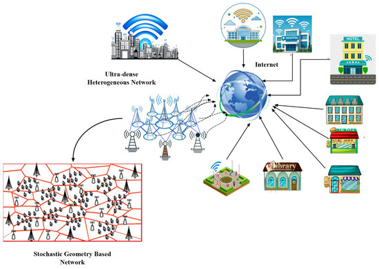
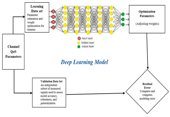
SG provides a probabilistic framework that models the spatial distribution of base stations and users in UDNs by employing random processes such as the Poisson Point Process (PPP). This approach enables the derivation of analytical performance metrics and closed-form expressions for key network parameters, making it particularly effective for interference analysis in large-scale deployments [5,13,14,15]. However, its applicability is constrained by assumptions of homogeneous node distributions and simplified propagation models, which may oversimplify the complexities of real-world network environments and non-uniform deployments [5,16,17,18,19]. Figure 1 illustrates the conceptual architecture of an UDN and its implementation using a SG-based heterogenous network model. At the top level, the network represents a densely deployed wireless environment composed of multiple tiers of base stations and access points serving diverse user locations and application scenarios. These include residential buildings, commercial areas, hospitals, hotels, libraries, and public spaces, all of which generate heterogeneous traffic demands with QoS requirements. At the core of the architecture lies the UDN, where macro base stations and a large number of small base stations coexist to provide seamless connectivity. The wireless access network is connected to the core network and the global Internet, enabling end-to-end communication and data exchange across different services and applications. To enable tractable performance analysis, the physical network is shown by a Voronoi Tessellation (VT) plot at the left bottom corner of the Figure 1. Here, base stations are spatially distributed according to a spatial point process, typically modeled using a PPP. The resulting VT represents the coverage regions of individual base stations, capturing the inherent randomness of node locations in UDN. Figure 1 represents the relationship between the real-world heterogeneous deployment and its analytical counterpart. This serves as the foundation for deriving key QoS metrics, which can subsequently be leveraged for simulation, optimization, and data-driven learning using ML and DL techniques.

1.2. From the Perspective of Machine Learning

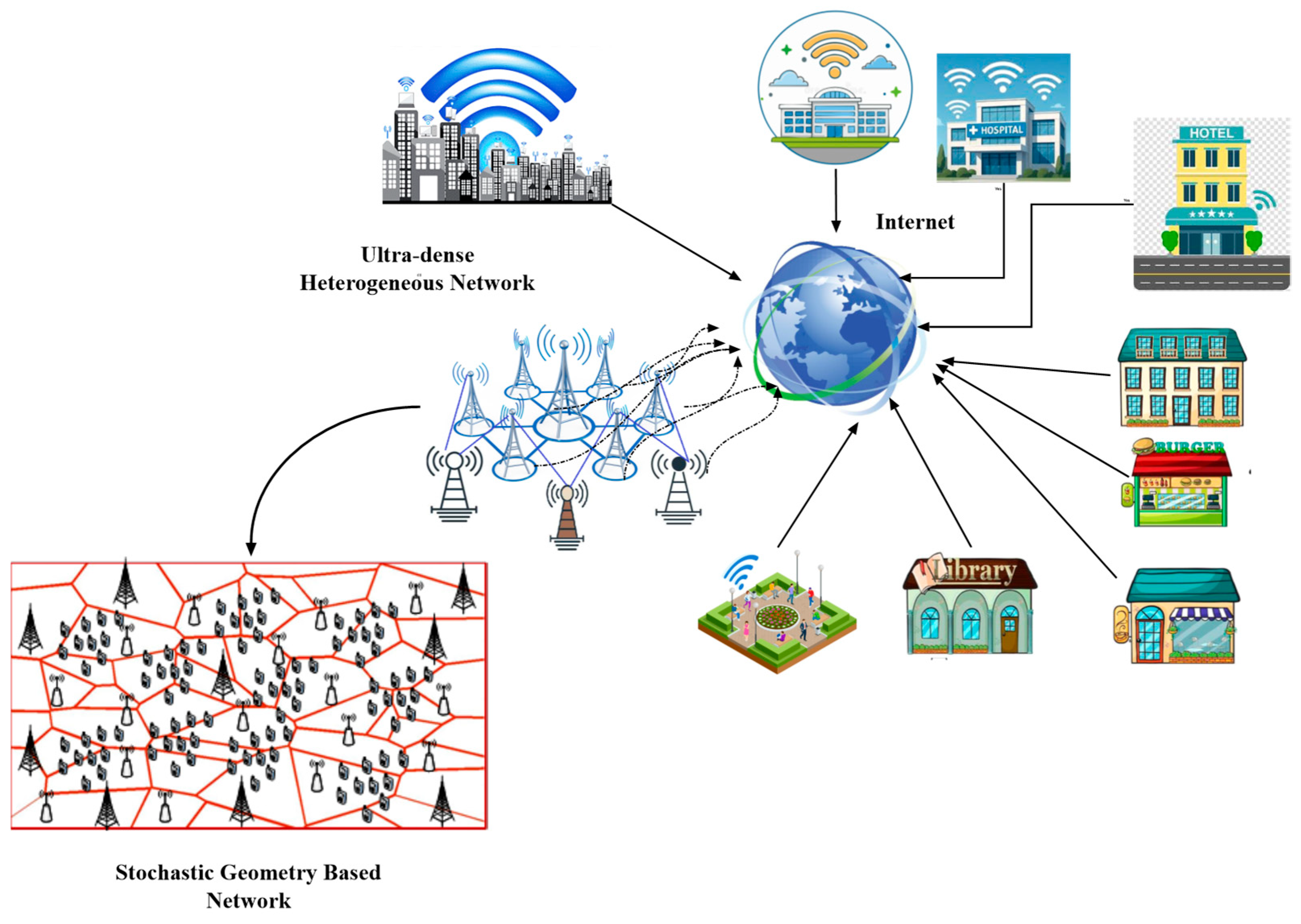
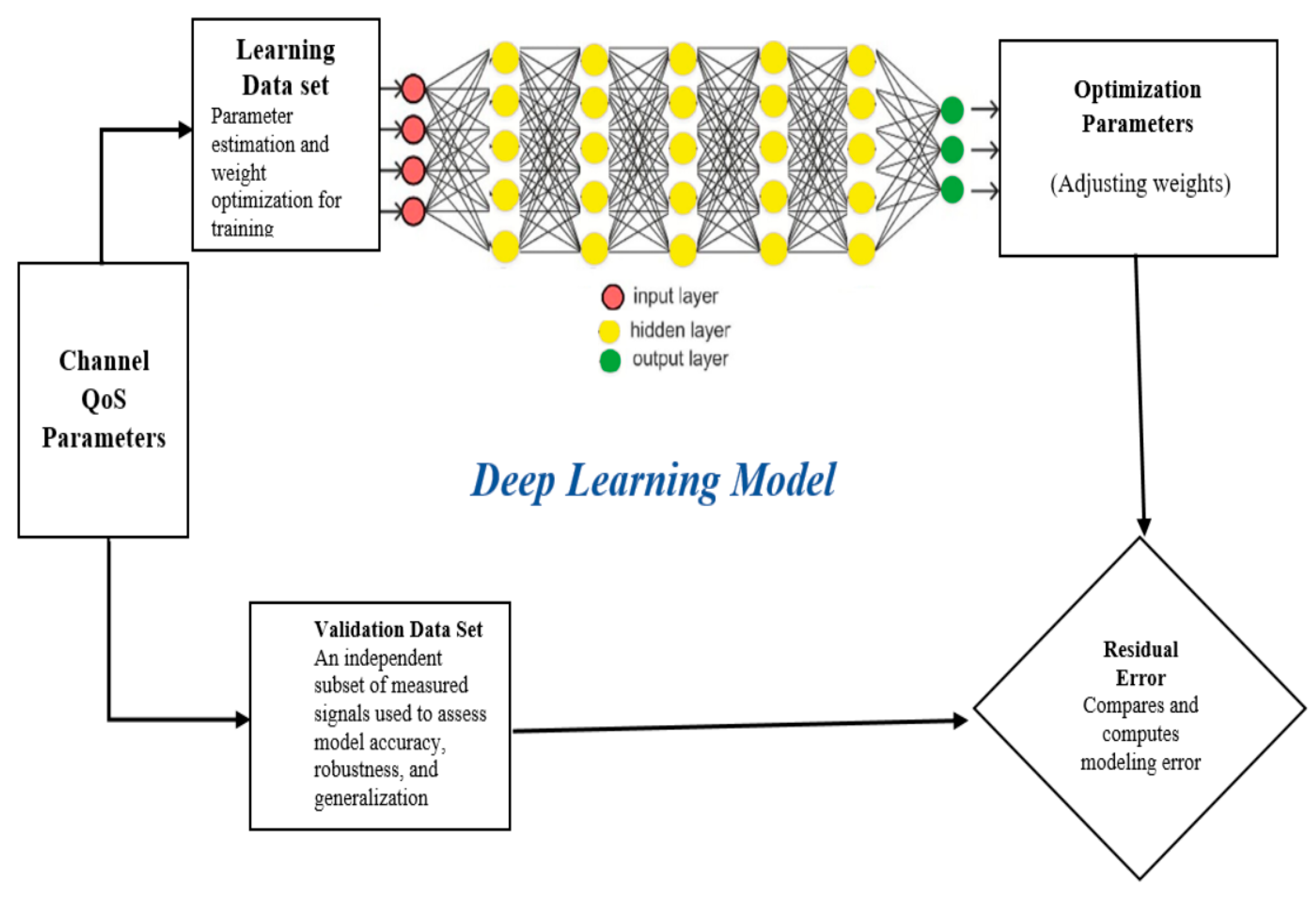
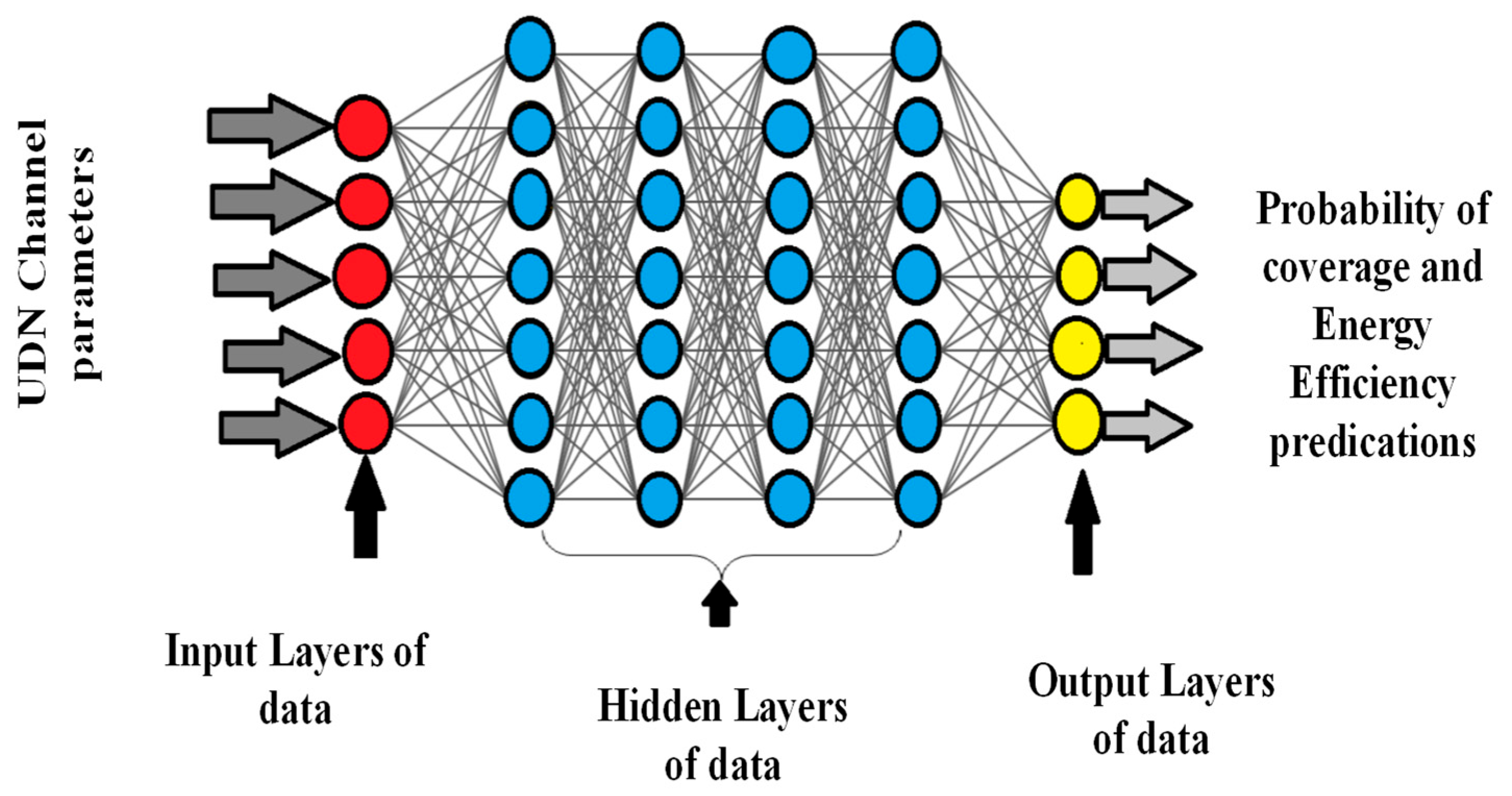
Conversely, ML methodologies offer a data-driven paradigm to enhance network modeling and optimization. These models exhibit significant capability in predicting network performance metrics, leveraging learned patterns from diverse data sources. ML’s inherent adaptability to heterogeneous network conditions and its ability to capture intricate network interactions contribute to improved accuracy across diverse and dynamic network scenarios [20,21]. Figure 2 illustrates the operational workflow of a ML-based DL network in a wireless communication system. QoS parameters obtained from the measurement system constitute the raw input data and represent the observed network behavior under varying conditions. These measurements are systematically organized into a learning dataset, which is used for model training, and a validation dataset. The processed data are then supplied to the DL architecture, consisting of an input layer, multiple hidden layers, and an output layer. Within the hidden layers, the network learns complex nonlinear relationships and underlying patterns among the QoS parameters through successive transformations. Finally, the effectiveness and reliability of the DL model are evaluated through error analysis, providing insight into its prediction accuracy and overall performance [10,22,23,24].

1.3. A Unified Approach Based on SG and ML

Unlike SG, which relies on fixed assumptions, ML techniques can dynamically adjust to changing network conditions and optimize operations. However, it may lack accuracy in representing the nuanced complexities of real world UDNs, as shown in Figure 1.

Table 1. Key challenges for SG-based and ML-based approaches [10,22,26].

S. No	Aspect	SG	Machine Learning (Including Deep Learning)
1.	Approach	Analytical, based on mathematical models and probability theory	Data-driven, learns patterns and relationships from data
2.	Nature of Analysis	Focus es on theoretical analysis and simulations	Focuses on learning from data, often using statistical models
3.	Modeling Characteristics	Uses probabilistic models to describe network elements and interactions	Utilizes algorithms to extract patterns and make predictions
4.	Input Requirements	Typically requires network parameters and assumptions (e.g., node density, path loss models)	Requires large amounts of labeled or unlabeled data for training
5.	Interpretability	Results are often interpretable in terms of theoretical network characteristics	Results can be complex and less interpretable, depending on model complexity and data
6.	Generalization	Captures general trends across network conditions	Adapts to specific data characteristics, potentially offering better predictive performance
7.	Scalability	Efficient for large-scale simulations with simplified assumptions	Requires computational resources for training large models
8.	Flexibility	Limited to scenarios described by mathematical models	Flexible in adapting to diverse and changing network environments
9.	Application Suitability	Suitable for initial network design and theoretical analysis	Suitable for real-world applications with diverse and dynamic data
10.	Challenges	May oversimplify real-world complexities and interactions	Requires careful preprocessing of data and tuning of models

summarizes the key aspects and challenges of using SG versus ML (including DL) for network modeling in UDNs based on references [4,5,20,21,23,25]. In continuation, the complementary strengths and limitations of SG and ML indicate that neither approach alone is sufficient for comprehensive QoS evaluation in UDNs. While SG offers analytical tractability and interpretability through closed-form expressions, it struggles to capture complex, nonlinear interactions arising from dense and heterogeneous deployments. Conversely, ML excels at learning such intricate relationships from data but often lacks physical interpretability and depends heavily on large, high-quality datasets. This motivates a hybrid framework in which SG is first utilized to model the spatial structure of the network and derive key QoS parameters under well-defined assumptions. By grounding data-driven learning in analytically derived features, the proposed approach aims to enhance prediction accuracy, reduce training complexity, and improve interpretability.

2. Literature Review

In recent research on UDNs, traditional clustering methods like K-means and graph-theory-based algorithms have been extensively studied alongside emerging deep-learning approaches. Traditional methods, such as K-means clustering, are favored for their simplicity but struggle with fixed cluster sizes and evenly distributed base stations. Graph theory-based algorithms, such as those employing max-degree and min-cut approaches, optimize energy efficiency by considering interference relationships among small base stations (SBSs) [27,28,29,30]. Conversely, DL-based clustering methods, including reinforcement learning and unsupervised learning, offer dynamic adaptation capabilities that adjust cluster formations based on real-time network conditions. Reinforcement-learning algorithms optimize network sum rate by allowing agents to learn optimal policies through interactions with their environment [31]. This adaptability is crucial in UDNs, where the distribution and density of base stations can vary significantly [22]. The heterogeneity of small cells in dense networks is achieved by optimizing energy saving and EE through sub channel allocation, sub frame configuration, and power allocation. The study proposes a heterogeneity aware optimization algorithm to ensure fairness and improve system EE while reducing energy consumption.

The authors in reference [32] present a joint interference suppression scheme using deep-reinforcement learning to maximize spectrum efficiency in heterogeneous networks with dense small cells. The study introduces a deep deterministic policy gradient (DDPG)-based algorithm to address power control and interference alignment, demonstrating improved performance compared to existing algorithms.

Traditional resource allocation methods typically rely on greedy algorithms or semi-definite programming to efficiently allocate sub channels and power [33,34]. The authors in reference [35] analyze the UDN using game theory approaches. While these methods are straightforward and computationally efficient, they may struggle with scalability and adapting to dynamic network changes. In contrast, DL-based resource allocation leverages neural networks to optimize complex objectives, such as energy efficiency and throughput maximization. Q-learning algorithms reduce computational complexity while dynamically allocating resources based on learned policies [20]. Centralized cooperative learning schemes using Q-tables enable agents to collaboratively optimize resource allocation strategies, effectively reducing interference and improving network efficiency [36]. Optimization objectives in traditional methods often focus on specific metrics, such as energy efficiency or throughput maximization, while considering QoS requirements [27,37,38,39]. These methods provide a structured approach but may lack adaptability to varying network conditions and optimization criteria. DL-based approaches offer a flexible framework to simultaneously optimize multiple objectives in UDNs. Reinforcement-learning frameworks allow agents to learn complex decision-making processes that optimize throughput, energy efficiency, and QoS metrics dynamically [38].

This capability is particularly advantageous in environments where conditions change rapidly and traditional static approaches may fall short. Both traditional and DL-based methods aim to address common challenges in UDNs, such as computational complexity, interference management, and dynamic adaptation.

Traditional methods excel in simplicity and initial implementation ease, but may struggle with scalability and handling large-scale data efficiently [22,31,40,41,42]. DL-based approaches mitigate these challenges by leveraging neural networks to handle large state-action spaces and complex decision-making processes. By adopting distributed cooperative learning and reinforcement learning techniques, these approaches reduce interference, optimize resource utilization, and improve overall network performance [33,36,40].

In summary, the literature review highlights the ongoing evolution of methodologies for clustering, resource allocation, and optimization in UDNs. Traditional methods provide a solid foundation but face limitations in adapting to dynamic environments and optimizing complex objectives simultaneously. DL-based approaches, leveraging reinforcement learning and neural networks, offer promising avenues to address these challenges by enabling adaptive, efficient, and scalable solutions for future UDN deployments [21,32,38,43].

Table 2. Methods and approaches in network optimization.

Aspect	Traditional Methods	ML Approaches	References
Clustering Methods	K-means clustering	Reinforcement learning, Q-learning, unsupervised learning	[22,33,38]
	Graph theory-based clustering (e.g., max-degree, min-cut)	None	[27,28,30,36]
	Game theory-based clustering	None	[35]
Resource Allocation	Greedy algorithms	Centralized cooperative learning (Q-table), reinforcement learning	[34,36]
	Two-step subchannel allocation, power allocation	Distributed cooperative learning	[30]
Optimization Objectives	Energy Efficiency (EE) optimization	Throughput maximization, EE optimization	[27,37,38]
	Throughput maximization considering QoS (e.g., data rate)	None	[27]
Challenges Addressed	Computational complexity, fixed cluster size	Large state-action space, dynamic adaptation, congestion management	[22,40,41,42]

presents a compilation of methods and approaches utilized in network optimization, encompassing both traditional and ML-based strategies. Traditional methods such as K-means clustering and greedy algorithms are compared with ML approaches, including reinforcement learning and distributed cooperative learning [44,45,46]. These methods address different optimization objectives, such as energy efficiency and throughput maximization, while tackling challenges like computational complexity and dynamic adaptation in network environments.

Recent reinforcement-learning-based optimization approaches, such as Soft Actor–Critic (SAC) and Deep Deterministic Policy Gradient (DDPG), have demonstrated strong performance in dynamic resource allocation and power control problems through online interaction with the environment. These methods rely on continuous exploration, reward-driven policy updates, and iterative training, which can incur high computational complexity and convergence variability in ultra-dense networks. In contrast, the proposed SG–ML framework follows an offline learning paradigm, where analytically derived and simulation-validated data are used to train a regression model. This enables deterministic, low-latency inference during deployment, avoids online exploration overhead, and provides greater interpretability through SG-based modeling. While SAC and DDPG are well suited for real-time adaptive control, the proposed approach is particularly advantageous for fast, scalable performance evaluation and energy efficiency optimization under QoS constraints.

Research Gap and Motivation

SG has been extensively used for UDN analysis due to its analytical tractability and ability to derive closed-form expressions. However, SG-based models rely on simplified assumptions such as homogeneous BS distributions, fixed activity states, and idealized channel models, which limit their applicability in realistic UDNs with heterogeneous active–inactive BS behavior and QoS constraints. In contrast, ML/DL methods enable scalable and fast performance prediction but are typically trained using simulation-only datasets and operate independently of SG-based analytical models. This disconnects results in limited interpretability, weak generalization, and lack of analytical validation. Existing studies largely treat SG and ML in isolation, or apply ML as a black-box substitute without systematically leveraging SG-derived metrics. To address this gap, this work proposes a unified SG–DL framework that integrates analytical modeling, Monte Carlo simulation, and DL. SG is used to model the UDN and derive SINR, coverage probability, and EE under QoS constraints. The analytical results are validated via simulations in MATLAB. EE optimization is performed through dynamic small cell BS activity control. Analytical and simulation-derived data are jointly used to train a DL model, enabling fast and accurate prediction of probability of coverage and EE for unseen UDN configurations.

3. System Model

3.1. Stochastic-Geometry-Based System Network Model

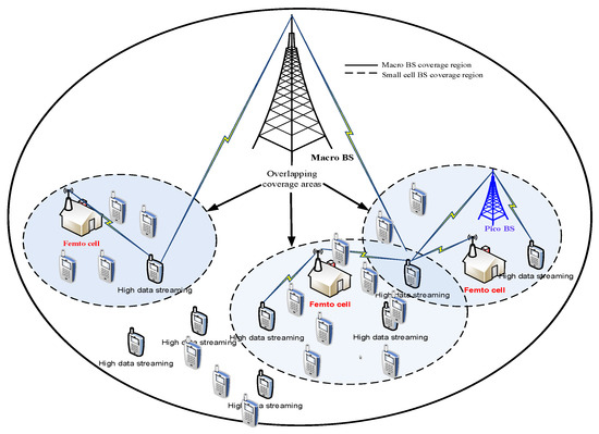
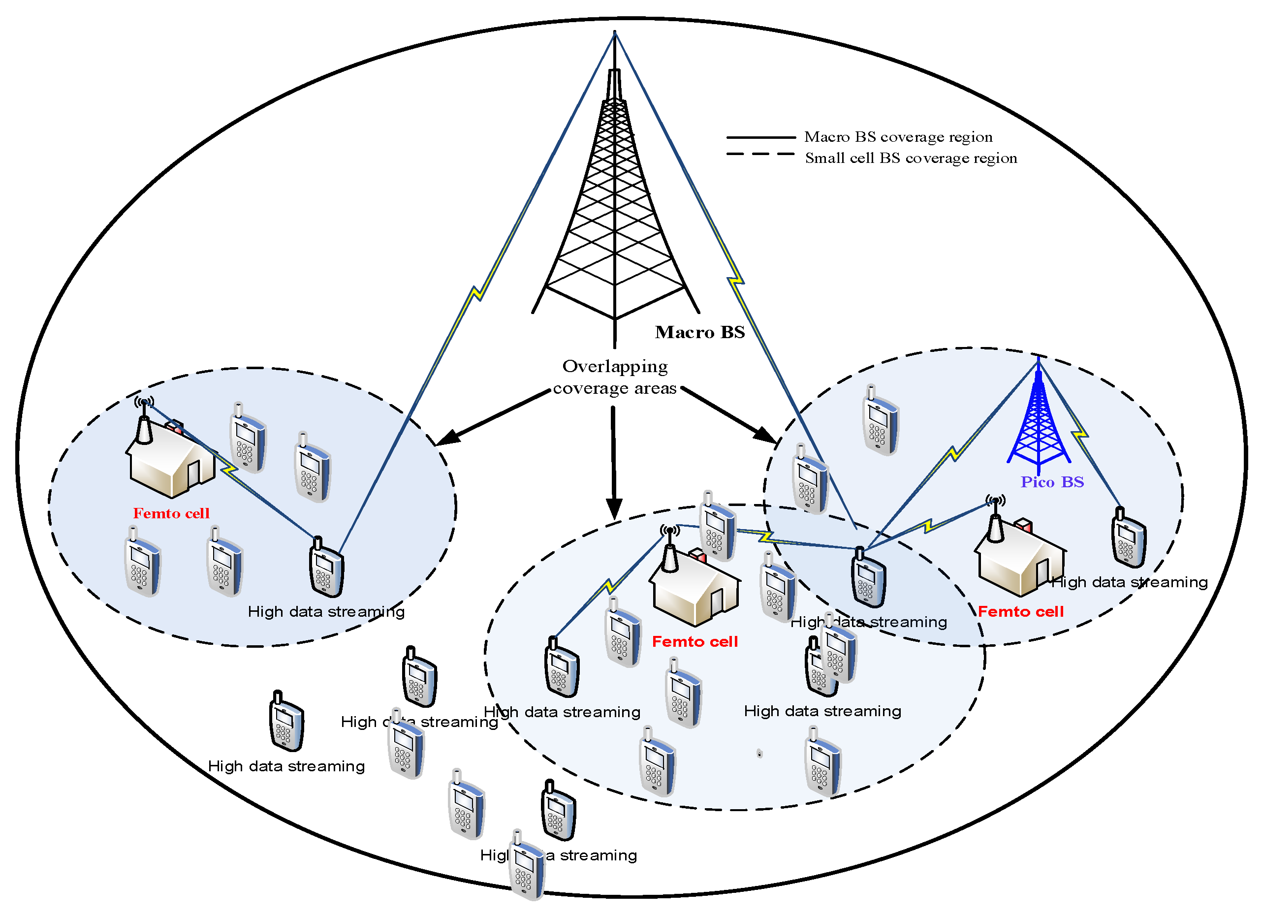
Figure 3 represents a UDN consisting of macro base stations distributed according to a homogeneous PPP ${\mathsf{\Theta }}_{\mathrm{M}}$ with a density ${\mathsf{\Lambda }}_{\mathrm{m}}$ in a Euclidean plane has been analyzed. Additionally, Femto (small) BSs and all mobile users (MUs) are randomly distributed in space, following two separate, homogenous and independent PPPs with densities ${\mathsf{\lambda }}_{\mathrm{f}}$ and ${\mathsf{\lambda }}_{\mathrm{u}}$, respectively (Figure 3).

The spatial densities, transmit powers, and path-loss parameters used in Figure 3 are consistently applied across all experiments. For validation, the analytical expressions are evaluated over a large number of independent spatial realizations, and the resulting coverage probability and energy efficiency metrics are averaged. These validated results are then organized into a supervised learning dataset, forming the validation pipeline illustrated in Figure 4, where simulation outputs are used to train and test the regression model.

SINR measures the quality of communication by comparing the power of the received signal from the serving BS with the interference from other BSs and background noise. Interference is generated by all BSs in the network, except the serving BS, reflecting the complex interactions within the network [21,47,48]. While the proposed framework is generalizable to such multi-tier UDNs, in this study we focus primarily on the macro–femto, which are the two tiers for tractability and clarity of analysis. This choice is motivated by the fact that femto cells typically dominate interference in dense deployments due to their high density and short-range operation.

In the femto tier, which consists of low-power BSs, sleep mode strategies are employed to manage energy consumption. These strategies determine whether a BS remains active or enters inactive (sleep) mode, affecting overall power consumption and network performance.

Network tiers vary in data rates, transmit power, and BS densities. For successful communication, the SINR must exceed a predefined threshold. The analysis is conducted for a MU located at the origin. Thus, any MU can connect to its nearest BS in the ith tier, provided the SINR at the MU exceeds the threshold. Each tier is characterized by parameters $\{{\mathrm{P}}_{\mathrm{i}},{\mathsf{\lambda }}_{\mathrm{i}},{\mathsf{\xi }}_{\mathrm{i}}\}$ where ${\mathrm{P}}_{\mathrm{i}}$ denotes the transmit power, ${\mathsf{\lambda }}_{\mathrm{i}}$ represents the BS density, and ${\mathsf{\xi }}_{\mathrm{i}}$ includes additional characteristics of the tier.

For ease of notation, consider a user positioned at the origin O, with all base stations situated relative to this point. The SIINR for a mobile user located at O during downlink transmission from a BS can be expressed as follows:

$${\mathrm{S}\mathrm{I}\mathrm{N}\mathrm{R}}_{(\mathrm{x}\to {\mathrm{M}\mathrm{U}}_{\mathrm{o}})}={\displaystyle \frac{{\mathrm{P}}_{\mathrm{t}\mathrm{x},\mathrm{i}}{\mathrm{h}}_{\mathrm{x}}{\mathrm{g}}_{\mathrm{x}}}{\sum _{\mathrm{i}=1}^{\mathrm{K}}{\sum }_{\mathrm{y}\in {\mathsf{\Theta }}_{\mathrm{x}}}{\mathrm{P}}_{\mathrm{t}\mathrm{x},\mathrm{y}}{\mathrm{h}}_{\mathrm{y}}{\mathrm{g}}_{\mathrm{y}}+{\mathsf{\sigma }}^2}}$$

(1)

In Equation (1), ${\mathsf{\Theta }}_{\mathrm{x}}$ represents the set of all interfering nodes with the MU at x, ${\mathrm{P}}_{\mathrm{t}\mathrm{x},\mathrm{i}}$ denotes the transmitted power of the femto BS at tier $\mathrm{i},$ and ${\mathrm{h}}_{\mathrm{x}}\mathrm{and}{\mathrm{h}}_{\mathrm{y}}$ are the channel gains from nodes x and y, respectively, due to small-scale fading. It is assumed that Rayleigh fading channel gains follow ${\mathrm{h}}_{\mathrm{x}}~\exp \left(1\right)$ and ${\mathrm{h}}_{\mathrm{y}}~\exp \left(1\right)$. The background noise is modeled as Additive White Gaussian Noise (AWGN) with variance${\mathsf{\sigma }}^2,$ and the path loss function is given by ${\mathrm{g}}_{\mathrm{x}}={‖\mathrm{x}‖}^{-\mathsf{\alpha }}$, where α is the path loss exponent.

In the power consumption model for femto base stations (BSs), the hardware design is a critical factor. Based on the design outlined in [12], the total power consumption ${\mathrm{P}}_{\mathrm{T}}$ of a femto BS is the sum of power used by the microprocessor ${\mathrm{P}}_{\mathrm{\mu }\mathrm{p}}$, the Field Programmable Gate Array, ${\mathrm{P}}_{\mathrm{F}\mathrm{P}\mathrm{G}\mathrm{A}}$, and the Power Amplifier, ${\mathrm{P}}_{\mathrm{P}\mathrm{A}}$.

$${\mathrm{P}}_{\mathrm{T}\mathrm{o}\mathrm{t}\mathrm{a}\mathrm{l}}=\left[{\mathsf{\Lambda }}_{\mathrm{m}}\cdot {\mathrm{P}}_{\mathrm{m}\mathrm{a}\mathrm{c}\mathrm{r}\mathrm{o}}\right]+\left[{\mathsf{\lambda }}_{\mathrm{f}}\cdot {\mathrm{P}}_{\mathrm{f}\mathrm{e}\mathrm{m}\mathrm{t}\mathrm{o}}\right]+{\mathrm{P}}_{\mathrm{P}\mathrm{A}}+{\mathrm{P}}_{\mathrm{\mu }\mathrm{p}}+{\mathrm{P}}_{\mathrm{F}\mathrm{P}\mathrm{G}\mathrm{A}}$$

(2)

In Equation (2), among these components, the RF (Radio Frequency) front end, which includes both the RF transmitter and receiver, is the most significant contributor to overall power usage, accounting for approximately 45% of the total consumption. The remaining portion of the power is consumed by the Temperature Compensated Crystal Oscillator (TCXO). Thus, the RF front end and TCXO together contribute to about 50% of the femto BS’s total power consumption. Notably, significant power savings can be achieved by turning off these RF components, which could potentially reduce power consumption by up to 50%, with minimal impact on the operation of the femto BS.

3.2. Deep-Learning-Based Model for Prediction

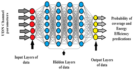
Figure 4 represents the second part of system model as DL-based system model for performance prediction in UDNs. Raw data collected from the UDN environment, including channel and network parameters such as BS density, channel conditions, transmit power, and SINR thresholds, serve as input features. In addition, QoS parameters obtained from network measurements are included to capture system behavior under diverse operating conditions.

The processed inputs are fed into a DL architecture consisting of an input layer, multiple hidden layers, and an output layer. The hidden layers learn nonlinear mappings and latent relationships between the input features and target performance metrics through successive feature transformations. The output layer produces estimates of network performance metrics, including coverage probability and energy efficiency. Model performance is evaluated using a validation dataset through error analysis, enabling quantitative assessment of prediction accuracy and generalization capability for unseen UDN scenarios.

Table 3. Performance analysis of a UDN using Stochastic Geometry and DL models [10,20,21,26,32,38].

Simulation Aspect	Analysis Using Stochastic Geometry	DL Analysis with Synthetic Training Patterns
Pros
Physics-based Understanding	Provides clear insights into physical network characteristics	Capable of learning intricate patterns and relationships
Interpretability	Results are interpretable and explainable	Flexibility in adapting to complex, real-world scenarios
Generalization Across Scenarios	Captures general trends across various network conditions	Improved accuracy with large, diverse datasets
Simplicity and Speed	Computationally efficient for simulations	Automatically extracts relevant features from raw data
Cons
Assumptions and Simplifications	Relies on idealized assumptions and may not reflect real-world complexity	Dependency on large amounts of labeled training data
Limited Complexity	May not capture complex, nonlinear interactions in dynamic networks	Potential challenges in interpreting learned features
Scalability Issues	Challenges scaling to large and dense networks	Initial setup and training may be computationally intensive

provides a comparative overview of the strengths and limitations of SG and DL for analyzing and simulating UDN performance. SG offers analytical tractability and physics-based interpretability, enabling efficient evaluation of key performance metrics under well-defined assumptions. However, it relies on simplified spatial and propagation models, which may limit its ability to capture complex interactions in dense and dynamic network environments. DL, in contrast, excels at learning intricate nonlinear relationships from data and adapting to heterogeneous scenarios, but requires large labeled datasets and incurs significant computational overhead during training. This comparison underscores the complementary nature of SG and DL, motivating their integration to balance analytical rigor with predictive flexibility in UDN performance analysis.

3.3. Hybrid SG–DL Algorithm for Performance Evaluation

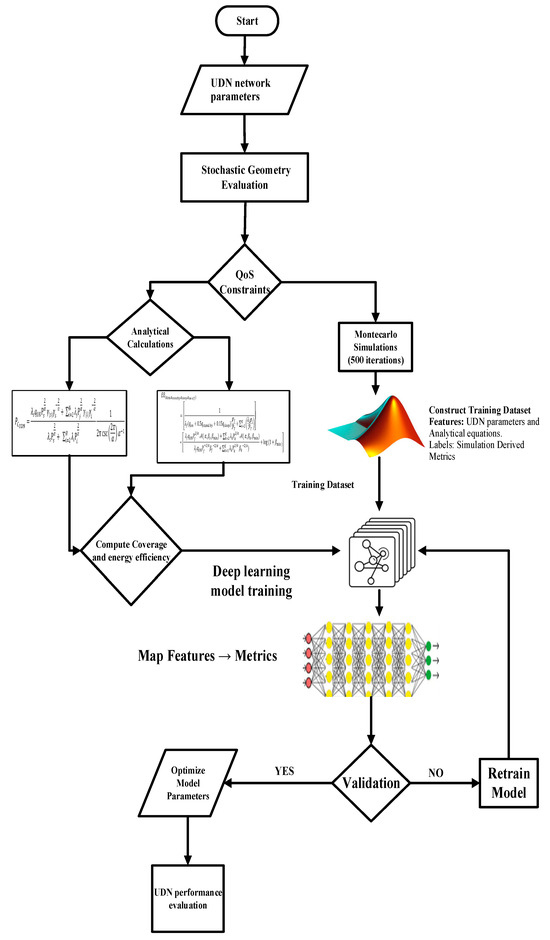
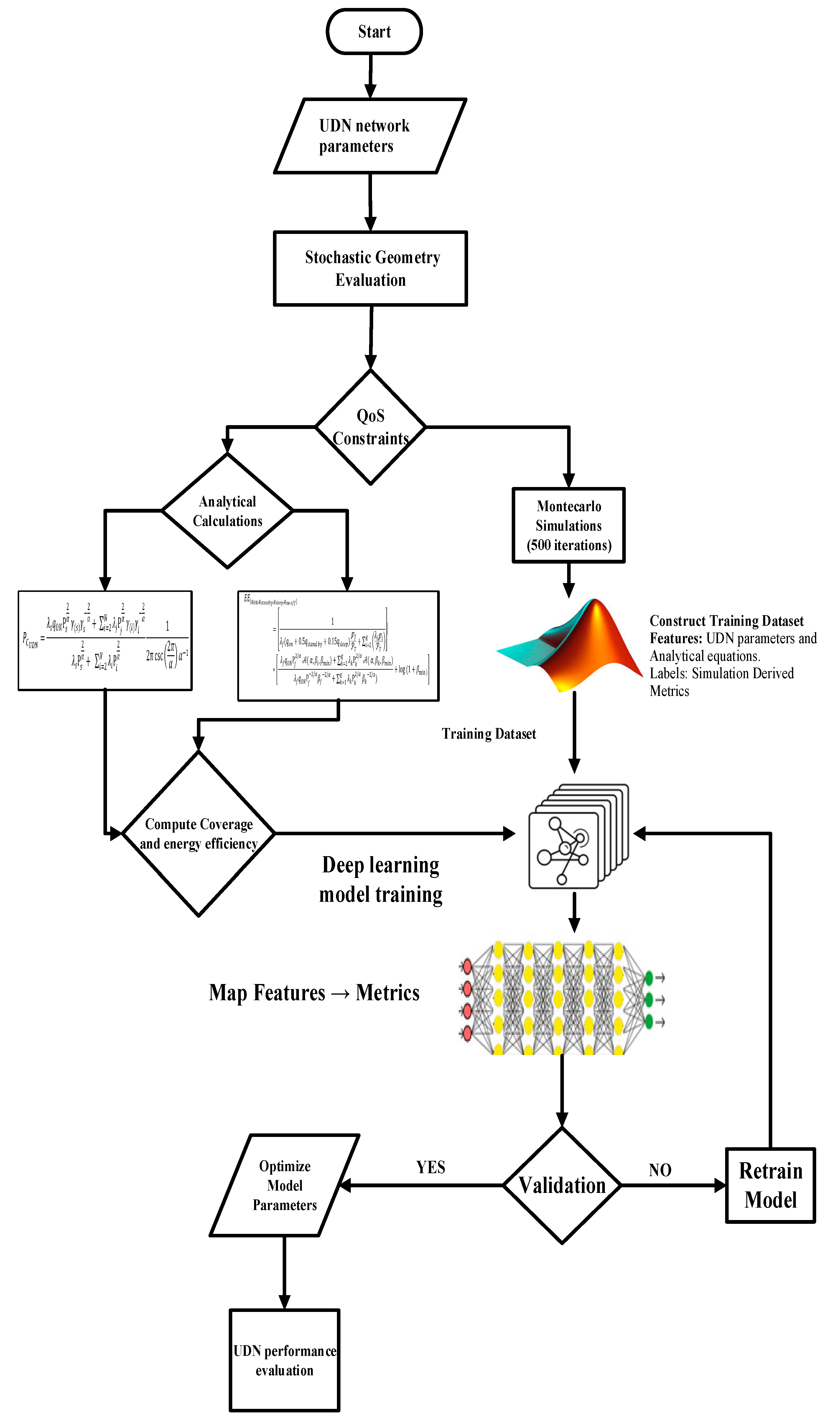
The proposed framework integrates SG-based Monte Carlo simulation and DL to enable efficient performance evaluation and energy-efficiency optimization in a UDN. The framework workflow is illustrated in the corresponding flowchart, as shown in Figure 5. The process begins with the specification of key UDN parameters, including BS density, user distribution, transmit power, the path–loss model, and QoS thresholds. These parameters are provided as inputs to the SG-based evaluation block, where the spatial randomness of BSs and mobile users is modeled using stochastic point processes. QoS constraints, such as SINR thresholds, are imposed to ensure realistic performance assessment. Based on these constraints, the framework proceeds along two parallel evaluation paths. In the SG-based analytical path, closed-form expressions for key performance metrics, including coverage probability and energy efficiency, are derived. In parallel, MC simulations are conducted to validate the analytical results by randomly deploying BSs and users under the same spatial assumptions. The outputs from the analytical and simulation paths are combined to construct a supervised learning dataset, consisting of network configuration parameters as input features and the corresponding performance metrics as target labels. This dataset is used to train a DL model that learns the nonlinear mapping between network features and performance outcomes, enabling rapid prediction of coverage and energy efficiency without repeated SG analysis or computationally intensive simulations. The trained DL model is subsequently validated to assess prediction accuracy and generalization capability. If the validation performance does not meet predefined criteria, the model is retrained with updated parameters. Once satisfactory performance is achieved, the optimized model is employed for final UDN performance evaluation and energy efficiency analysis.

Although the workflow in Figure 5 illustrates a generic data-driven learning architecture, the implemented learning model in this study is based on supervised SVR. The term “DL-based framework” is used in a broad sense to denote data-driven learning integrated with SG rather than a deep neural network trained online. SVR is selected due to its stable convergence, low training complexity, and strong generalization capability for small- to medium-sized datasets derived from analytically grounded SG models. The core contribution therefore lies in the integration of SG with supervised learning for scalable and fast performance prediction, rather than in the design of a specific deep neural network architecture.

In this section, we develop a mathematical framework based on SG to analyze EE and PC, formulating the problem to maximize EE under QoS constraints. The model is then used to train a DL model via Monte Carlo simulations for data-driven optimization.

4. Mathematical Preliminaries for Stochastic Geometry

4.1. Point Processes (PP)

A Point Process (PP) is a stochastic model used to describe the spatial arrangement of random points in a given region. This model is highly effective for analyzing random spatial distributions. In the realm of UDN, a Point Process models the spatial distribution of base stations or other network elements in a two-dimensional plane. A Point Process is typically defined as a measurable mapping $\Phi$ from a separable space $R^d$ (where $d\ge 1$) to the set of positive integers. This mapping is locally finite and represents the spatial distribution of points.

4.2. Poisson Point Processes (PPPs)

Point Processes can be categorized into different types, including Simple Point Processes, Stationary Point Processes (SPPs), Non-Stationary Point Processes, and Poisson Point Processes (PPPs). For this study, we focus on Simple PPs, SPPs, and PPPs, which are defined as follows:

• A Simple Point Process ensures that each spatial location contains at most one point, preventing overlap of points within the Euclidean space.
• A Stationary Point Process maintains statistical invariance under translation, meaning its properties are consistent across different spatial locations.
• The Poisson Point Process (PPP) is a widely used model in Stochastic Geometry. A PPP is characterized by:
  • Independence of points in disjoint regions.
  • Poisson distribution of the number of points within any given region $A\in R^d$ with the mean proportional to the measure of $A$

The probability of observing a point in region A is given by:

$$\mathsf{{\rm P}}\left(\mathrm{N}\left(\mathrm{A}\right)=\mathrm{a}\right)={\displaystyle \frac{{\left(\eta \left(A\right)\right)}^a{e}^{-\eta \left(A\right)}}{a!}}$$

(3)

In Equation (3), $\eta \left(A\right)$ represents the measure of the region $A$. In this study, we use a homogeneous PPP, where the point density remains constant across the entire spatial domain, making it suitable for analyzing the spatial distribution in UDNs.

In our proposed network model, the base station is distributed as PPPs with specified densities, such as a macro base station density of 0.5 and densities of interfering small cells (0.3 and 0.2). The simulation evaluates key metrics like $P_C$ and $EE$. This modeling framework enables the assessment of network performance under different conditions of transmit powers (e.g., $P_f=10 \mathrm{d}\mathrm{B}$), channel gains (e.g., ${\beta }_f$ = 1.0) for macro base stations, ${\beta }_i$ = [1.2, 1.5] for interfering cells, and other network parameters. These findings, derived from a stochastic geometry framework with PPP-based network modeling, provide actionable insights for network planning, interference management, and resource allocation in wireless communication systems. They contribute to the design of more resilient and energy-efficient networks, catering to diverse user demands and operational environments.

5. Coverage Probability Using SG Analysis

A MU is considered to be in the coverage area of a BS when its average SINR, ${\gamma }_{\left(avg\right)}$, exceeds a certain threshold value, ${\gamma }_{\left(Th\right)}$. This implies that the MU can connect to at least one BS with an SINR greater than the threshold value. With this understanding, the coverage probability for a small cell under UDN is derived for the open-access mode.

In an interference-limited environment where self-interference is the dominant factor over internal noise, the probability of coverage for a typical MU can be expressed as [6]

$$\begin{gathered} P_{C_{UDN}}={\displaystyle \frac{{\lambda }_s{q}_{ON}{\mathrm{P}}_s^{\frac{2}{\alpha }}{\gamma }_{\left(s\right)}{\gamma }_s^{-\frac{2}{\alpha }}+\sum _{i=2}^N{\lambda }_j{\mathrm{P}}_j^{\frac{2}{\alpha }}{\gamma }_{\left(i\right)}{\gamma }_i^{-\frac{2}{\alpha }}}{{\lambda }_s{\mathrm{P}}_s^{\frac{2}{\alpha }}+\sum _{i=2}^N{\lambda }_i{\mathrm{P}}_i^{\frac{2}{\alpha }}}}{\displaystyle \frac{1}{2\pi \csc \left(\frac{2\pi }{\alpha }\right){\alpha }^{-1}}}; \\ Where\left\{\begin{array}{c}{\gamma }_{\left(s\right)}>{\gamma }_{\left(Th\right)}>{\gamma }_{\left(i\right)}>1\\ \end{array}\right. \end{gathered}$$

(4)

In Equation (4), $P_{C_{UDN}}$ represents the coverage probability of a typical mobile user in an UDN. The variable ${\lambda }_s$ denotes the density of small base stations, while $q_{ON}$ indicates the fraction of these small BSs that are active at any given time. The term $P_s$ signifies the transmit power of these small cells, and α is the path loss exponent, reflecting how signal strength diminishes with distance. γ is the SINR threshold required for coverage from small cells. For other types of base stations, ${\lambda }_i$ denotes their density, $P_i$is their transmit power, and $\gamma$ is the SINR threshold for coverage from these base stations. The sum $\sum _{i=2}^N{\lambda }_j{\mathrm{P}}_j^{{\displaystyle \frac{2}{\alpha }}}{\gamma }_{\left(i\right)}{\gamma }_i^{-{\displaystyle \frac{2}{\alpha }}}$ accounts for the aggregate contribution to coverage probability from all types of BSs, excluding small cells, while $\sum _{i=2}^N{\lambda }_i{\mathrm{P}}_i^{{\displaystyle \frac{2}{\alpha }}}$ represents the total interference from these base stations. The normalization factor ${\displaystyle \frac{1}{2\pi \csc \left(\frac{2\pi }{\alpha }\right){\alpha }^{-1}}}$ adjusts the coverage probability based on the spatial distribution of base stations and the path loss characteristics. This factor accounts for the geometric and probabilistic aspects of the network, ensuring that the coverage probability reflects the overall network configuration accurately.

To illustrate the operational validity of the proposed analytical framework, a single-tier UDN scenario is first considered for clarity and analytical tractability. Monte Carlo simulations were conducted in MATLAB with over 500 independent realizations, and the simulated coverage probability exhibits close agreement with the analytical results, thereby validating the correctness of the derived expression. This preliminary single-tier analysis serves to demonstrate the underlying behavior of the model. The detailed simulation-based performance evaluation, including coverage probability and energy efficiency (EE) for multi-tier UDN deployments, is presented and discussed in the subsequent section.

6. Problem Formulation Based on SG Analysis

One of the prime objectives in UDN is to maximize the Energy Efficiency while maintaining the QoS constraints. Using the tools from SG, the optimization problem is formulated by jointly considering the operational states of small-cell BSs (active, standby, sleep, and switched-off), where EE is defined as the ratio of achievable spectral efficiency to total network power consumption. The optimization is subject to constraints ensuring that (i) the coverage probability exceeds a predefined threshold, (ii) the SINR at a typical user remains above the required SINR threshold, and (iii) the probabilities of BS operational states are valid and bounded. The resulting SG-based analytical solution provides the maximum achievable EE under QoS constraints, which is subsequently used to generate labeled data for training a DL model. The DL model learns the nonlinear relationship between network parameters and EE, enabling fast and scalable prediction of optimal EE for unseen UDN configurations. Therefore, our goal is to maximize

$${EE}_{(q_{ON},q_{standby},q_{sleep},q_{swoff})}=\left[{\displaystyle \frac{1}{{{\lambda }_f(q}_{on}+0.5q_{standby}+0.15q_{sleep})\frac{{\mathcal{p}}_f}{{\mathcal{P}}_T}+\sum _{i=2}^K\left(\frac{{{\lambda }_i\mathcal{p}}_i}{{\mathcal{P}}_T}\right)}}\right]\mathrm{*}\left[\left.{\displaystyle \frac{{\lambda }_f{q}_{ON}{\mathrm{P}}_f^{2/\alpha }\mathcal{A}(\alpha ,{\beta }_i,{\beta }_{min})+\sum _{k=2}^K{\lambda }_k{\mathrm{P}}_k^{2/\alpha }\mathcal{A}(\alpha ,{\beta }_k,{\beta }_{min})}{{\lambda }_f{q}_{ON}{\mathrm{P}}_f^{-2/\alpha }{{\beta }_f}^{-2/\alpha }+\sum _{k=1}^K{\lambda }_k{\mathrm{P}}_k^{2/\alpha }{{\beta }_k}^{-2/\alpha })}}+\mathrm{l}\mathrm{o}\mathrm{g}(1+{\beta }_{\mathrm{m}\mathrm{i}\mathrm{n}})\right]\right.$$

Subject to

$$\begin{gathered} {0\le q}_{on}+q_{standby}+q_{sleep}+q_{sw.off}\le 1 \\ {\gamma }_{\left(s\right)}>{\gamma }_{\left(Th\right)}>{\gamma }_{\left(i\right)}>1 \\ \mathrm{and} \\ {P}_{C_{ON}}={\displaystyle \frac{{\lambda }_f{q}_{ON}{\mathrm{P}}_f^{2/\alpha }{\beta }_f^{-2/\alpha }+\sum _{j=2}^K{\lambda }_i{\mathrm{P}}_i^{2/\alpha }{\beta }_i^{-2/\alpha }}{{\lambda }_f{\mathrm{P}}_f^{2/\alpha }+\sum _{j=2}^K{\lambda }_i{\mathrm{P}}_i^{2/\alpha }}}{\displaystyle \frac{1}{2\pi \mathrm{c}\mathrm{s}\mathrm{c}\left(\frac{2\pi }{\alpha }\right){\alpha }^{-1}}}>{\beta }_{Th} \\ \left\{\begin{array}{c}{\mathsf{\beta }}_{f_{average}}<{\beta }_{Th}\\ {\mathsf{\beta }}_{macro}>1\end{array}\right. \end{gathered}$$

(5)

In Equation (5), the variables of interest are $q_{on},q_{standby},q_{sleep},$ and $q_{sw.off}$ and the optimal solution would be the maximized EE with the QoS requirement being satisfied.

γ is the SINR threshold required for coverage from small cells. For other types of base stations, ${\lambda }_i$ denotes their density, $P_i$ is their transmit power, and $\gamma$ SINR threshold for coverage from these base stations. The sum

$$\sum _{i=2}^N{\lambda }_j{\mathrm{P}}_j^{{\displaystyle \frac{2}{\alpha }}}{\gamma }_{\left(i\right)}{\gamma }_i^{-{\displaystyle \frac{2}{\alpha }}}$$

accounts for the aggregate contribution to coverage probability from all types of BSs, excluding small cells, while

$$\sum _{i=2}^N{\lambda }_i{\mathrm{P}}_i^{{\displaystyle \frac{2}{\alpha }}}$$

represents the total interference from these base stations.

7. Algorithm Design

This Algorithm 1 describes the SVM training model. It calculates Coverage Probability and Energy Efficiency for different scenarios using specified formulas. The data is prepared for SVM training, with SINR values and parameters used as inputs (X) and $P_c$/EE values as outputs (Y). It splits the data for training and validation, trains SVM regression models for $P_c$ and EE, predicts values, evaluates with residuals, and plots results, including $P_c$ vs. SINR, EE vs. SINR, scatter plots of actual vs. predicted values, and residual analysis.

Algorithm 1: Training Model

Input: Initialize simulation parameters: Set values for ${\lambda }_f,{\lambda }_i,P_f,{\beta }_{min},{\beta }_i,q_{ON},\mathrm{and}{\beta }_{th}$ for different path loss exponents. Initialization: Generate SINR values Create an array ‘SINR values’ ranging from 0 to 20 dB. Initialize result arrays: Create $P_c$values and ‘EE values’ as empty arrays to store calculated results. Calculate Coverage Probability ($P_c$) and Energy Efficiency (EE). iteration: Iterate over each ‘α’ value. For each α, iterate over ‘SINR values’ Calculate $P_c$ based on conditions involving ${\lambda }_f$, ${\lambda }_i$, $P_f$, ${\beta }_{min}$, and ${\beta }_i$. Compute EE using formulas with for ${\lambda }_f$, ${\lambda }_i$, $P_f$, ${\beta }_{min}$, ${\beta }_i$, $q_{ON}$, and ${\beta }_{th}$. Store computed $P_c$and EE values in$P_c$values and EE values, respectively. Prepare data for SVM training: Create input-output pairs (X, Y, $P_c$, X’Y, EE) for SVM regression. Combine SINR values and α values into X. Populate Y, $P_c$ with $P_c$ values and Y, EE with EE values. Split data for training and validation: Use hold-out cross-validation (cv partition) to divide data into training (X train, Y, $P_c$ train, EE train). Validation sets (X values, Y, $P_c,$values, Y, EE values). Train SVM models: Train an SVM regression model (SVM, $P_c$) using X train, Y, $P_c$ train, EE train. Train another SVM regression model (SVM, EE) using X train, Y, $P_c$ train, EE train. Predict and evaluate models: Predict $P_c$ and EE using trained SVM models and X train. Calculate residuals (residuals, $P_{c,}$ and residuals, EE) by subtracting predicted values from actual values. Plot results: Plot $P_c$ vs. SINR for each α separately. Plot EE vs. SINR for each α separately. Plot scatter plots of actual vs. predicted $P_c$ and EE. Plot residuals of $P_c$ and EE predictions to analyze model performance. End

8. Results Analysis from the SG-Based Framework

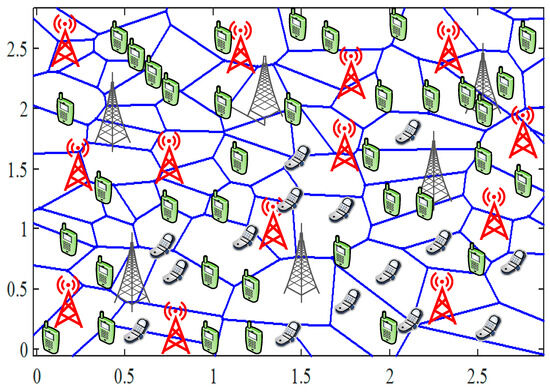
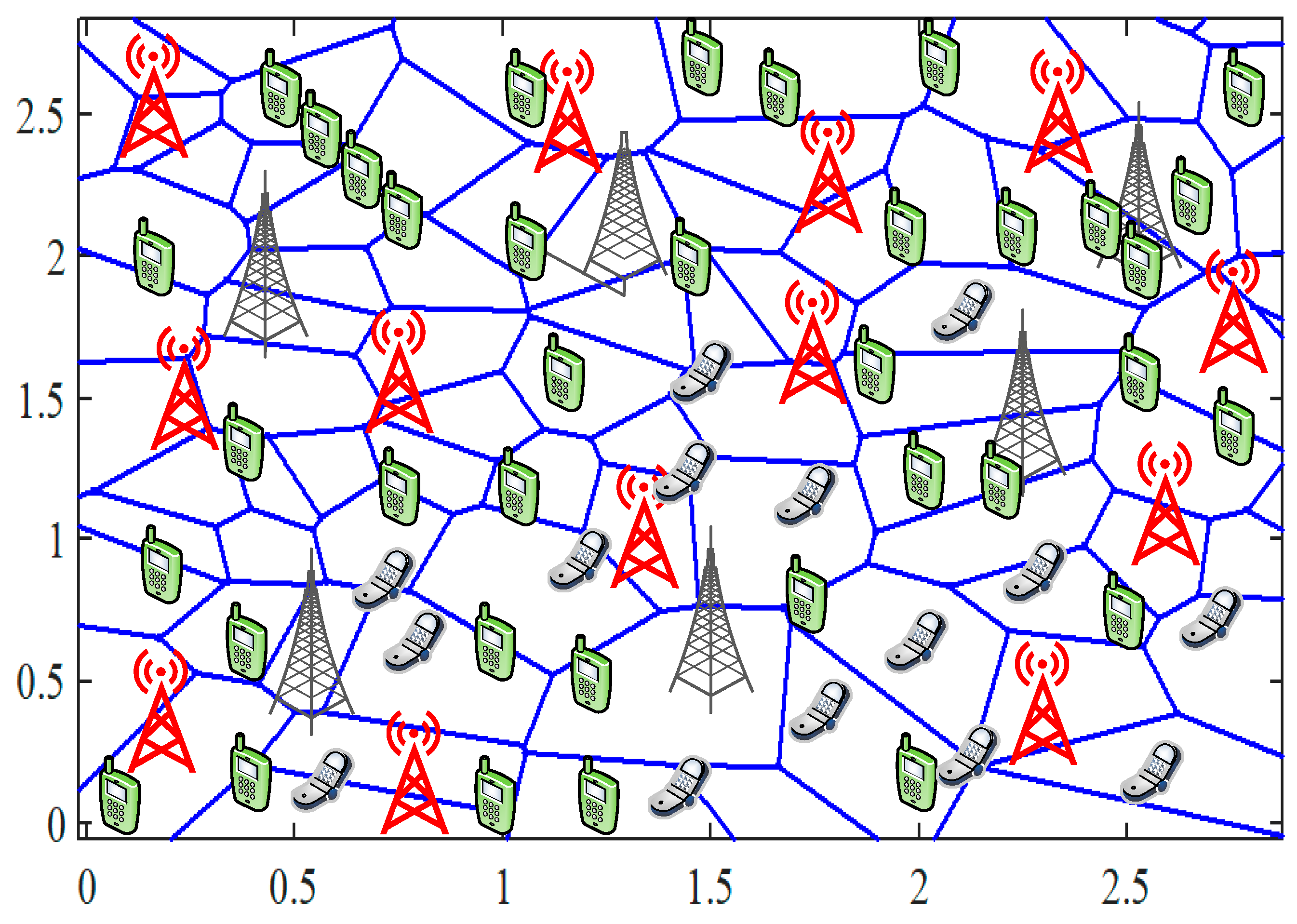
SG is used to model the spatial distribution of base stations and users in UDNs. Poisson Voronoi tessellations are employed for cell association and mobility modeling, as shown in Figure 6.

MU is considered to be in the coverage region when it can transmit/receive signals to/from its nearest BSs. With sleep mode schemes, the expression for coverage probability is similar to that without sleep mode, with the density of active small BSs being ${\lambda }_s{q}_{on}$.

This leads to the following equation:

$$\begin{gathered} P_{C_{UDN}}=ActiveSmallcelltier{BS}_{EnergyEfficient}+Sumofallothertiers \\ {P}_{C_{UDN}}={\displaystyle \frac{{\lambda }_s{q}_{ON}{\mathrm{P}}_f^{\frac{2}{\alpha }}{\gamma }_s^{-\frac{2}{\alpha }}+\sum _{i=2}^N{\lambda }_i{\mathrm{P}}_i^{\frac{2}{\alpha }}{\gamma }_i^{-\frac{2}{\alpha }}}{{\lambda }_s{\mathrm{P}}_s^{\frac{2}{\alpha }}+\sum _{i=2}^N{\lambda }_i{\mathrm{P}}_i^{\frac{2}{\alpha }}}}{\displaystyle \frac{1}{2\pi \csc \left(\frac{2\pi }{\alpha }\right){\alpha }^{-1}}}; \\ \mathrm{w}\mathrm{h}\mathrm{e}\mathrm{r}\mathrm{e}\left\{\begin{array}{c}{\gamma }_s>{\gamma }_{Th}\\ \end{array}\right.{\gamma }_j>1 \end{gathered}$$

(6)

The UDN coverage probability is defined by the analytical expression given in Equation (5). For explicit numerical evaluation, the contribution of the active small cell tier is computed as

$$\begin{gathered} {\lambda }_s{q}_{ON}{P}_f^{\left\{{\displaystyle \frac{2}{\alpha }}\right\}{\gamma }_s^{\left\{-{\displaystyle \frac{2}{\alpha }}\right\}}} \\ =0.005\times 7.07\times {2.2}^{\left\{-0.5\right\}}\approx 0.0374 \end{gathered}$$

similarly, the macro base station tier contribution is obtained as

$$\begin{gathered} {\lambda }_m{P}_m^{\left\{{\displaystyle \frac{2}{\alpha }}\right\}{\gamma }_m^{\left\{-{\displaystyle \frac{2}{\alpha }}\right\}}} \\ =0.01\times 22.36\times {1.3}^{\left\{-0.5\right\}}\approx 0.0241 \end{gathered}$$

By summing these terms, the numerator of the coverage probability in Equation (4) is

$$\begin{gathered} =\mathrm{Active}\mathrm{small}\mathrm{cell}+\mathrm{Macro}\mathrm{tier} \\ ={\lambda }_s{q}_{ON}{\mathrm{P}}_f^{{\displaystyle \frac{2}{\alpha }}}{\gamma }_s^{-{\displaystyle \frac{2}{\alpha }}}+{\sum }_{i=2}^N{\lambda }_i{\mathrm{P}}_i^{{\displaystyle \frac{2}{\alpha }}}{\gamma }_i^{-{\displaystyle \frac{2}{\alpha }}} \\ =0.0374+0.0241\approx 0.0615 \end{gathered}$$

The active small cell power term and macro BS power term are:

$$=0.001\times 22.36\approx 0.0224$$

The corresponding denominator, representing the total transmit power contribution of all tiers, is calculated as

$$\begin{gathered} \mathrm{Active} \mathrm{small} \mathrm{cell}+\mathrm{Macro} \mathrm{tier} \\ ={\lambda }_s{\mathrm{P}}_s^{{\displaystyle \frac{2}{\alpha }}}+{\sum }_{i=2}^N{\lambda }_i{\mathrm{P}}_i^{{\displaystyle \frac{2}{\alpha }}} \\ =0.0354+0.0224\approx 0.0578 \end{gathered}$$

Substituting the numerator and denominator values into Equation (4) yields the final coverage probability for the single-tier UDN scenario.

$$\begin{gathered} P_{C_{UDN}}={\displaystyle \frac{{\lambda }_s{q}_{ON}{\mathrm{P}}_f^{\frac{2}{\alpha }}{\gamma }_s^{-\frac{2}{\alpha }}+\sum _{i=2}^N{\lambda }_i{\mathrm{P}}_i^{\frac{2}{\alpha }}{\gamma }_i^{-\frac{2}{\alpha }}}{{\lambda }_s{\mathrm{P}}_s^{\frac{2}{\alpha }}+\sum _{i=2}^N{\lambda }_i{\mathrm{P}}_i^{\frac{2}{\alpha }}}}{\displaystyle \frac{1}{2\pi \csc \left(\frac{2\pi }{\alpha }\right){\alpha }^{-1}}} \\ ={\displaystyle \frac{0.0615}{0.0578}}\times 0.637\approx 0.678 \end{gathered}$$

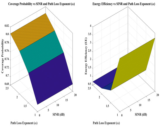
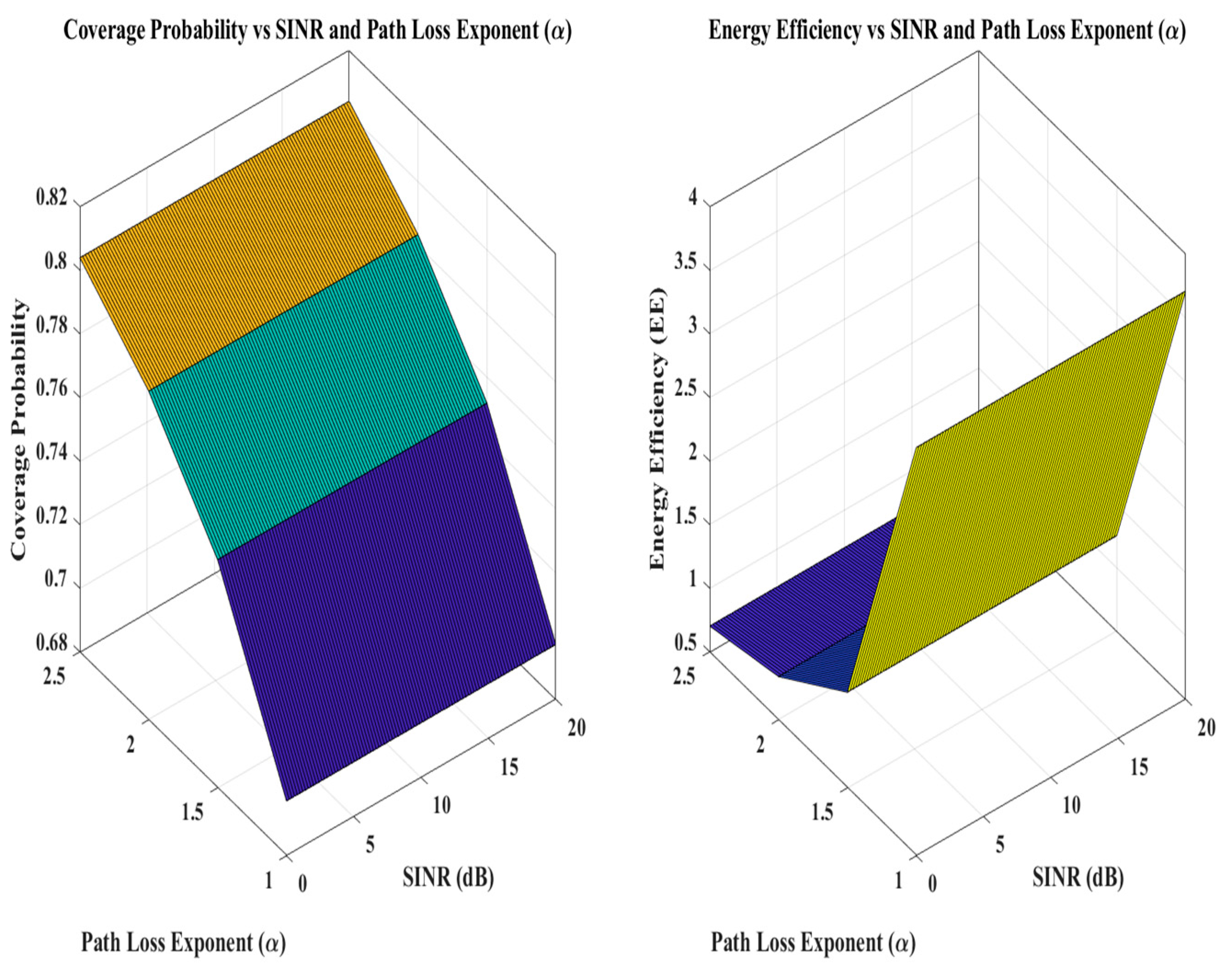
Figure 7 (left side), shows that coverage probability increases with SINR. Moreover, the dependency of $P_C$ on the path loss exponent (α), ranging from 1.0 to 2.5, underscores the impact of signal propagation characteristics on coverage performance. Coverage probability measures the likelihood that a mobile user (MU) can establish a reliable connection with at least one BS, ensuring adequate Signal-to-Interference Ratio (SIR) levels. The parameters of the simulation are listed in

Table 4. Simulation parameters for Stochastic Geometry.

Parameter	Value(s)
$\mathrm{Femto}\mathrm{BS}\mathrm{density}\left({\mathsf{\lambda }}_{\mathrm{f}}\right)$	0.5
$\mathrm{Interfering}\mathrm{BS}\left({\mathsf{\lambda }}_{\mathrm{i}}\right)$	[0.3, 0.2]
$\mathrm{Transmit}\mathrm{Power}\left({\mathrm{P}}_{\mathrm{f}}\right)$	10
Path Loss Exponents (α)	[1.0, 1.5, 2.0, 2.5]
SINR Range	0 dB to 20 dB
Thresholds	${\mathsf{\beta }}_{\mathrm{m}\mathrm{i}\mathrm{n}}$$=0.5,{\mathsf{\beta }}_{\mathrm{T}\mathrm{h}}$= 0.7
Other Parameters	${\mathsf{\beta }}_{\mathrm{f}}$$=0.8,{\mathsf{\beta }}_{\mathrm{m}\mathrm{a}\mathrm{c}\mathrm{r}\mathrm{o}}$= 1.1

.

9. Results Analysis from the DL-Based Framework

The SG-based analytical model is used to compute EE and coverage probability under QoS constraints for different UDN configurations. The analytically obtained results are used to construct a labeled dataset. Network parameters, including BS densities, transmit powers, activity probabilities, and SINR thresholds, are used as input features, while EE and coverage probability serve as target outputs. A supervised SVM regression model is trained using this dataset. Model performance is evaluated by comparing actual and predicted EE and coverage probability through scatter plots and residual analysis.

The dataset employed for training SVR models was generated using SG-based analytical formulations validated through Monte Carlo simulations. It comprises SINR values in the range of 0–20 dB and path loss exponents (α) ∈ {1.0, 1.5, 2.0, 2.5}. For each (SINR, α) pair, the corresponding $P_C$ and EE were computed using the SG formulations described in the system model (Equations (4)–(6)).

As a result, the dataset contains four structured attributes:

(a)

SINR [dB]: an independent input feature representing the received signal quality;

(b)

Path loss exponent (α): an independent input reflecting the propagation environment;

(c)

Pc: a dependent output representing coverage probability;

(d)

EE: a dependent output representing energy efficiency.

In total, the dataset comprises 80 distinct data samples, generated across 20 SINR levels (0–20 dB, 1 dB resolution) and four path–loss exponents (α = {1.0, 1.5, 2.0, 2.5}). Each data point represents the empirical mean of 10³ Monte Carlo realizations, ensuring statistical stability and reproducibility. The dataset was partitioned into training and validation subsets, ensuring that the predictive models were evaluated on unseen data points to assess generalization. In

Table 5. Simulation parameters for DL.

SINR (dB)	Actual (dB)	$\mathbf{Actual}{\mathit{P}}_{\mathit{C}}$	$\mathbf{Predicted}{\mathit{P}}_{\mathit{C}}$	Actual EE	Predicted EE
5.0	1.0	0.75	0.74	0.85	0.86
10.0	1.5	0.65	0.66	0.75	0.76
15.0	2.0	0.55	0.54	0.65	0.64
20.0	2.5	0.45	0.46	0.55	0.54

, the SVR predictions show close agreement with analytical values, with low residual errors.

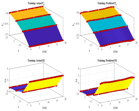
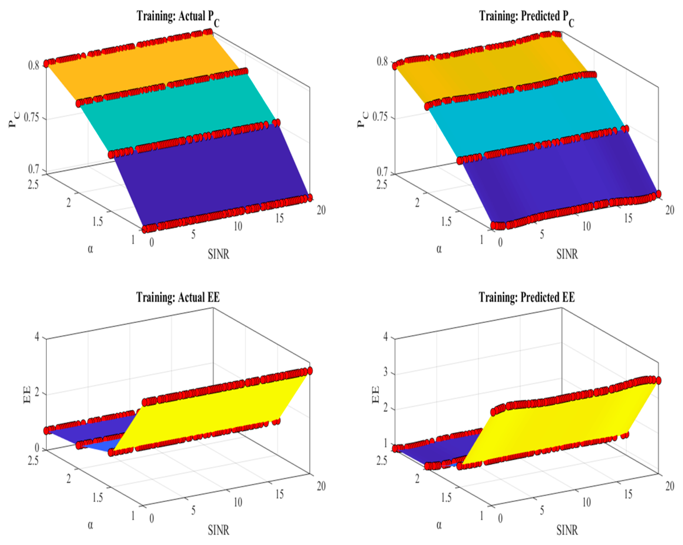
In the residual distribution notably, $P_C$ decreases as SINR increases, a trend accurately captured by the SVM model. These data points illustrate how the models predict coverage probability and EE for specific SINR and α values (Figure 8).

For EE, the values demonstrate a similar trend, where the model’s predictions closely match the actual values. This highlights the model’s effectiveness in EE. Moreover, EE decreases with increasing SINR and α. The model captures this relationship effectively, providing reliable predictions.

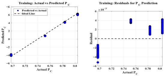
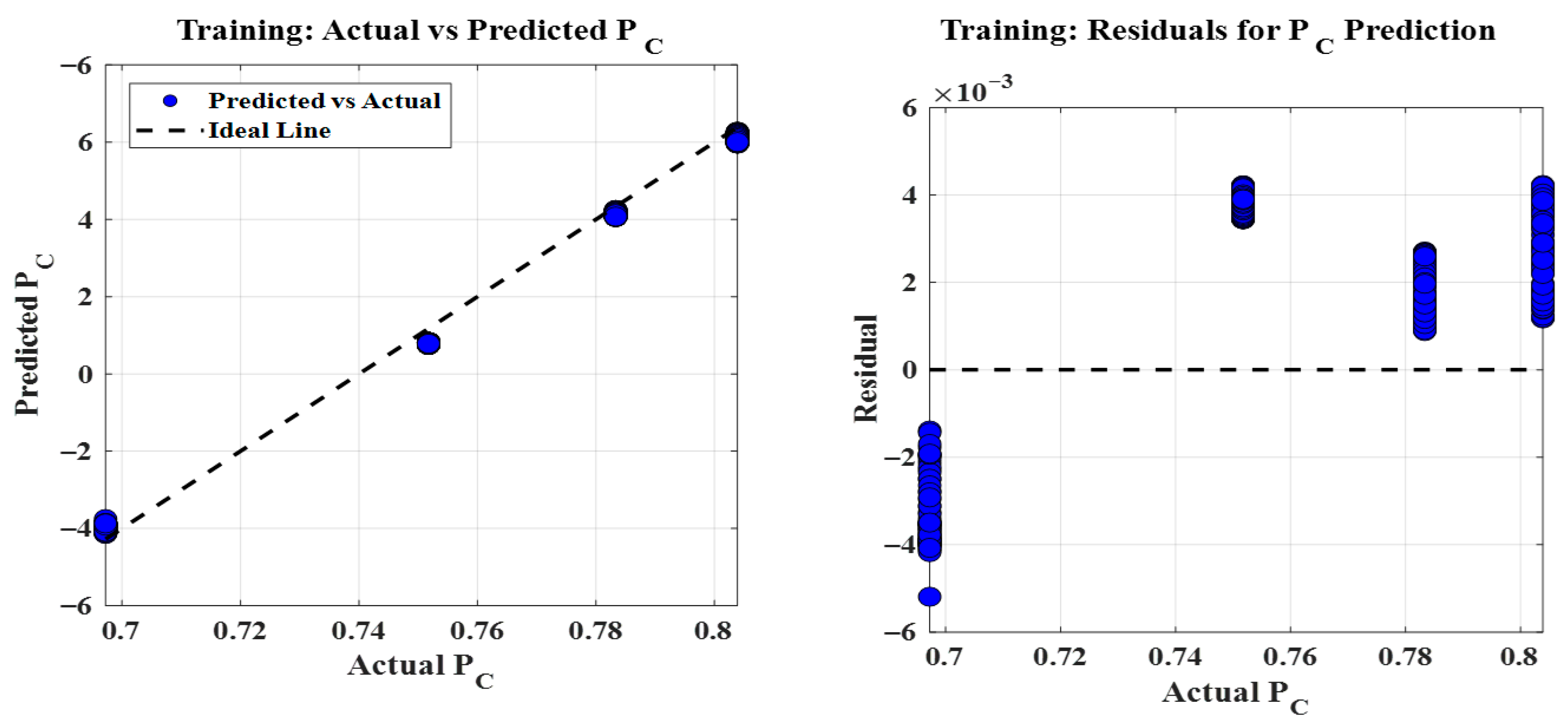
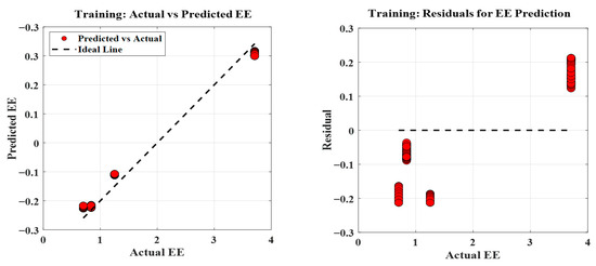
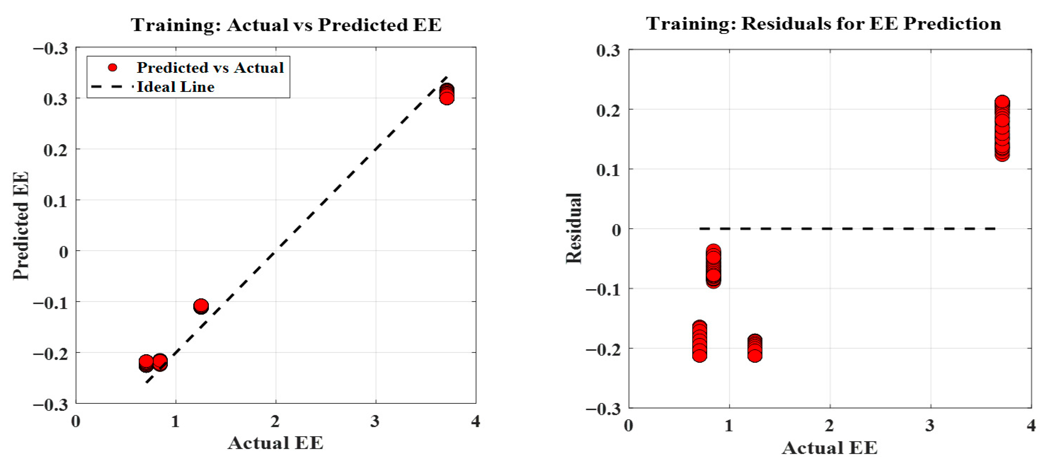
Residual analysis, as shown in Figure 9 and Figure 10, reveals that residuals for both $P_C$ and EE are evenly distributed around zero. The 3D surface plots the smooth variation of $P_C$ and EE across different SINR and α values. The close alignment between the actual and predicted surfaces in these plots. In summary, the SVM regression models for $P_C$ and EE demonstrate high accuracy and robustness, effectively capturing the complex relationships between SINR, the path–loss exponent, and the respective performance metrics. Figure 9 and Figure 10 illustrate the residual prediction analysis for Pc and EE, respectively. The ideal reference line at residual = 0 corresponds to perfect alignment between actual ($y$) and predicted ($\widehat{y}$) values, where residuals are defined as

$$r=y-\widehat{y}$$

For an accurate model, residuals should satisfy $E\left[r\right]\approx 0$ and $Varr\left(r\right)$.

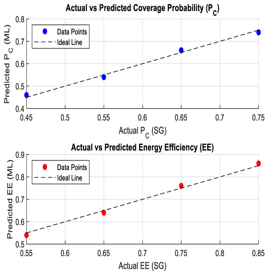
In our case, the residuals for both coverage and EE are symmetrically distributed around zero, with a maximum deviation $\left|r\right|\le 0.02$|r| (≤±2%). The mean residual is approximately zero $({\mu }_r\approx 0$) and the variance is negligible. This indicates that the SVR models achieve high fidelity in predicting both metrics. From a generalization standpoint, an under fitted model (high bias) would exhibit structured residuals deviating consistently from the zero line, while an over fitted model (high variance) would show near-zero error on training data but unstable, scattered residuals when applied to unseen data. By contrast, the results in Figure 9 and Figure 10 show residuals concentrated tightly around zero for all SINR–α combinations. Furthermore, the associated 3D surfaces exhibit monotonic and smooth variations: coverage decreases from 0.75 $\alpha =1.0\mathrm{to}0.45$ at α = 2.5, and EE decreases from 0.85 to 0.55 across the same range. This quantitative agreement confirms that the SVR models capture the nonlinear dependence of coverage and EE on SINR and α. Collectively, both results validate that the regression framework achieves residual error margins within ±2%.

The proposed framework focuses on fast performance prediction rather than continuous real time control. The SG analysis and simulations are used to construct a regression model, while the prediction stage relies on SVR inference involving kernel evaluations. As a result, the execution time per prediction is on the order of milliseconds on standard computing platforms, introducing negligible computational overhead and making the approach suitable for scalable deployment.

10. Integrated Analysis of the SG- and DL-Based Models

The unified approach for $P_C$ and EE across different path loss exponents (α), reveals insightful findings. According to the stochastic geometry simulations, actual $P_C$ values gradually decrease as α increases. For instance, $P_C$ decreases from 0.75 at α = 1.0 to 0.45 at α = 2.5. Similarly, EE decreases with higher α from 0.85 at α = 1.0 to 0.55 at α = 2.5.

The SVM regression models closely predict $P_C$ and EE values, with discrepancies between actual and predicted results consistently minimal (around 0.01). This demonstrates the SVM model’s high accuracy in capturing the complex relationships between SINR, α, and network performance metrics. Both approaches effectively capture the decreasing trends of $P_C$ and EE as α increases.

SVM regression leverages empirical data to make accurate predictions. Figure 11 represents the analysis of error margins between SG simulations and ML predictions for $P_C$ and EE across different path loss exponents (α). The percentage errors calculated show minimal deviations between the ML-predicted values and the actual values obtained from SG simulations. For $P_C$, the errors range from −1.82% to 2.22%, indicating that the ML model generally predicts $P_C$ values close to the actual SG results, with slight overestimations or underestimations. Similarly, EE exhibits percentage errors ranging from −1.54% to 1.33%, suggesting that the ML model effectively captures the trends in EE across varying α values, as shown in

Table 6. Comparison of actual and predicted values with percentage errors.

α	$\mathbf{Actual}{\mathit{P}}_{\mathit{C}}$ (SG)	$\mathbf{Predicted}{\mathit{P}}_{\mathit{C}}$ (ML)	$\%\mathbf{Error}{\mathit{P}}_{\mathit{C}}$	Actual EE (SG)	Predicted EE (ML)	% Error EE
1.0	0.75	0.74	−1.33	0.85	0.86	1.18
1.5	0.65	0.66	1.54	0.75	0.76	1.33
2.0	0.55	0.54	−1.82	0.65	0.64	−1.54
2.5	0.45	0.46	2.22	0.55	0.54	−1.82

.

11. Conclusions

This work proposed a scalable optimization framework for UDN by integrating stochastic-geometry-based analytical modeling with deep-learning-driven prediction. Stochastic geometry was employed to characterize network behavior and derive QoS aware expressions for coverage probability and energy efficiency under key system parameters, including base station density, transmit power, activation probability, and SINR thresholds. These analytical outcomes enabled the construction of a structured dataset used to train a supervised deep-learning model. The trained DL model effectively learned the complex, nonlinear mapping between network configurations and performance metrics, enabling fast and accurate prediction of coverage probability and energy efficiency for unseen UDN scenarios. Compared to conventional SG-based numerical evaluations, the proposed framework significantly reduces computational complexity while maintaining analytical consistency and QoS compliance. Overall, the integrated SG–DL approach highlights how the two components complement each other and provide a scalable tool for performance evaluation and energy optimization of a UDN, where purely analytical or simulation-based methods become computationally less efficient.

References

- Fadoul, M.M.; Gismalla, M.S.; Elshafie, H. A stochastic geometry approach for relay-assisted uplink multicell networks. Comput. Netw. 2025, 269, 111319. [Google Scholar] [CrossRef] [Scilit]
- Ngo, H.Q.; Interdonato, G.; Larsson, E.G.; Caire, G.; Andrews, J.G. Ultradense cell-free massive MIMO for 6G: Technical overview and open questions. Proc. IEEE 2024, 112, 805–831. [Google Scholar] [CrossRef] [Scilit]
- Mughees, A.; Tahir, M.; Sheikh, M.A.; Ahad, A. Energy-efficient ultra-dense 5G networks: Recent advances, taxonomy and future research directions. IEEE Access 2021, 9, 147692–147716. [Google Scholar] [CrossRef] [Scilit]
- Andrews, J.G.; Gupta, A.K.; Alammouri, A.; Dhillon, H.S. An Introduction to Cellular Network Analysis Using Stochastic Geometry; Springer: Durham, NC, USA, 2023. [Google Scholar]
- Ardanuc, M.; Basaran, M.; Hmamouche, Y.; Durak-Ata, L.; Yanikomeroglu, H. Energy efficiency analysis in heterogeneous networks: A stochastic geometry perspective. IEEE Open J. Veh. Technol. 2023, 4, 438–443. [Google Scholar] [CrossRef] [Scilit]
- Shabbir, A.; Rizvi, S.; Alam, M.M.; Shirazi, F.; Su’ud, M.M. Optimizing energy efficiency in heterogeneous networks: An integrated stochastic geometry approach with novel sleep mode strategies and QoS framework. PLoS ONE 2024, 19, e0296392. [Google Scholar] [CrossRef] [Scilit]
- Perdomo, J.; Gutierrez-Estevez, M.A.; Zhou, C.; Monserrat, J.F. WirelessNet: An Efficient Radio Access Network Model based on Heterogeneous Graph Neural Networks. IEEE Access 2025, 13, 36006–36023. [Google Scholar] [CrossRef] [Scilit]
- Fadoul, M.M.; Chow, C.-O. Half-duplex and full-duplex interference mitigation in relays assisted heterogeneous network. PLoS ONE 2023, 18, e0286970. [Google Scholar] [CrossRef] [Scilit]
- Armeniakos, H.K.; Bithas, P.S.; Tegos, S.A.; Kanatas, A.G.; Karagiannidis, G.K. Stochastic Geometry for Modeling and Analysis of Sensing and Communications: A Survey. IEEE Commun. Surv. Tutor. 2025, 28, 2691–2724. [Google Scholar] [CrossRef] [Scilit]
- Banerjee, B. Machine Learning and Stochastic Geometry Techniques for Future Mobile Communications. 2023. Available online: https://ualberta.scholaris.ca/server/api/core/bitstreams/a7836717-d12c-41b1-9036-a32b1fad4e1f/content (accessed on 1 September 2025).
- Hmamouche, Y.; Benjillali, M.; Saoudi, S.; Yanikomeroglu, H.; Di Renzo, M. New trends in stochastic geometry for wireless networks: A tutorial and survey. Proc. IEEE 2021, 109, 1200–1252. [Google Scholar] [CrossRef] [Scilit]
- Olotu, S.I. Stochastic Geometry and Federated Learning in Computational Modeling of Communication Systems. In Computational Modeling and Simulation of Advanced Wireless Communication Systems; CRC Press: New York, NY, USA, 2024; pp. 340–366. [Google Scholar]
- Ayoubi, R.A.; Spagnolini, U. Performance of dense wireless networks in 5G and beyond using stochastic geometry. Mathematics 2022, 10, 1156. [Google Scholar] [CrossRef] [Scilit]
- Nassar, H.; Taher, G.; El-Hady, E.S. Stochastic geometric modelling and simulation of cellular systems for coverage probability characterization. arXiv 2021, arXiv:2109.14063. [Google Scholar] [CrossRef] [Scilit]
- Ouamri, M.A. Stochastic geometry modeling and analysis of downlink coverage and rate in small cell network. Telecommun. Syst. 2021, 77, 767–779. [Google Scholar] [CrossRef] [Scilit]
- Hossain, M.A.; Hossain, A.R.; Ansari, N. AI in 6G: Energy-efficient distributed machine learning for multilayer heterogeneous networks. IEEE Netw. 2022, 36, 84–91. [Google Scholar] [CrossRef] [Scilit]
- Zhou, B.; Saad, W. Performance analysis of age of information in ultra-dense Internet of Things (IoT) systems with noisy channels. IEEE Trans. Wirel. Commun. 2021, 21, 3493–3507. [Google Scholar] [CrossRef] [Scilit]
- Li, L.; Cheng, Q.; Xue, K.; Yang, C.; Han, Z. Downlink transmit power control in ultra-dense UAV network based on mean field game and deep reinforcement learning. IEEE Trans. Veh. Technol. 2020, 69, 15594–15605. [Google Scholar] [CrossRef] [Scilit]
- Stoynov, V.; Poulkov, V.; Valkova-Jarvis, Z.; Iliev, G.; Koleva, P. Ultra-dense networks: Taxonomy and key performance indicators. Symmetry 2022, 15, 2. [Google Scholar] [CrossRef] [Scilit]
- Rathod, T.; Tanwar, S. AI-based resource allocation techniques in D2D communication: Open issues and future directions. Phys. Commun. 2024, 66, 102423. [Google Scholar] [CrossRef] [Scilit]
- Ahmad, I.; Hussain, S.; Mahmood, S.N.; Mostafa, H.; Alkhayyat, A.; Marey, M.; Abbas, A.H.; Rashed, Z.A. Co-Channel Interference Management for Heterogeneous Networks Using Deep Learning Approach. Information 2023, 14, 139. [Google Scholar] [CrossRef] [Scilit]
- Jiang, F.; Zhang, L.; Sun, C.; Yuan, Z. Clustering and resource allocation strategy for D2D multicast networks with machine learning approaches. China Commun. 2021, 18, 196–211. [Google Scholar] [CrossRef] [Scilit]
- Lopez-Perez, D.; De Domenico, A.; Piovesan, N.; Xinli, G.; Bao, H.; Qitao, S.; Debbah, M. A survey on 5G radio access network energy efficiency: Massive MIMO, lean carrier design, sleep modes, and machine learning. IEEE Commun. Surv. Tutor. 2022, 24, 653–697. [Google Scholar] [CrossRef] [Scilit]
- Pivoto, D.G.S.; de Figueiredo, F.A.P.; Cavdar, C.; Tejerina, G.R.d.L.; Mendes, L.L. A comprehensive survey of machine learning applied to resource allocation in wireless communications. IEEE Commun. Surv. Tutor. 2025, 28, 1986–2053. [Google Scholar] [CrossRef] [Scilit]
- Ye, M.; Fang, X.; Du, B.; Yuen, P.C.; Tao, D. Heterogeneous federated learning: State-of-the-art and research challenges. ACM Comput. Surv. 2023, 56, 1–44. [Google Scholar] [CrossRef] [Scilit]
- Wang, R.; Lou, Z.; Hu, L.; Wang, D.; Alouini, M.-S. How Stochastic Geometry and Machine Learning Coexist in Wireless Networks: Collaboration or Competition? In Proceedings of the AAAI 2025 Workshop on Artificial Intelligence for Wireless Communications and Networking (AI4WCN), Philadelphia, PA, USA, 3–4 March 2025. [Google Scholar]
- Sun, Y.; Guo, G.; Zhang, S.; Xu, S.; Wang, T.; Wu, Y. A cluster-based energy-efficient resource management scheme with QoS requirement for ultra-dense networks. IEEE Access 2020, 8, 182412–182421. [Google Scholar] [CrossRef] [Scilit]
- Qin, C.; Tian, H. A greedy dynamic clustering algorithm of joint transmission in dense small cell deployment. In Proceedings of the 2014 IEEE 11th Consumer Communications and Networking Conference (CCNC), Las Vegas, NA, USA, 10–13 January 2014; IEEE Press: Piscataway, NJ, USA, 2014; pp. 629–634. [Google Scholar]
- Laughlin, L.; Zhang, C.; Beach, M.A.; Morris, K.A.; Haine, J. A widely tunable full duplex transceiver combining electrical balance isolation and active analog cancellation. In Proceedings of the 2015 IEEE 81st Vehicular Technology Conference (VTC Spring), Glasgow, UK, 11–14 May 2015; IEEE Press: Piscataway, NJ, USA, 2015; pp. 1–5. [Google Scholar]
- Tian, X.; Jia, W. Improved clustering and resource allocation for ultra-dense networks. China Commun. 2020, 17, 220–231. [Google Scholar] [CrossRef] [Scilit]
- Zhang, L.; Peng, J.; Zheng, J.; Xiao, M. Intelligent cloud-edge collaborations assisted energy-efficient power control in heterogeneous networks. IEEE Trans. Wirel. Commun. 2023, 22, 7743–7755. [Google Scholar] [CrossRef] [Scilit]
- Wang, C.; Deng, D.; Xu, L.; Wang, W.; Gao, F. Joint interference alignment and power control for dense networks via deep reinforcement learning. IEEE Wirel. Commun. Lett. 2021, 10, 966–970. [Google Scholar] [CrossRef] [Scilit]
- Abdelnasser, A.; Hossain, E.; Kim, D.I. Clustering and resource allocation for dense femtocells in a two-tier cellular OFDMA network. IEEE Trans. Wirel. Commun. 2014, 13, 1628–1641. [Google Scholar] [CrossRef] [Scilit]
- Li, W.; Zhang, J. Cluster-based resource allocation scheme with QoS guarantee in ultra-dense networks. Iet Commun. 2018, 12, 861–867. [Google Scholar] [CrossRef] [Scilit]
- González, C.C.; Pupo, E.F.; Iradier, E.; Angueira, P.; Murroni, M.; Montalban, J. Network Selection over 5G-Advanced Heterogeneous Networks Based on Federated Learning and Cooperative Game Theory. IEEE Trans. Veh. Technol. 2024, 73, 11862–11877. [Google Scholar] [CrossRef] [Scilit]
- Lu, C.; Bao, Q.; Xia, S.; Qu, C. Centralized reinforcement learning for multi-agent cooperative environments. Evol. Intell. 2024, 17, 267–273. [Google Scholar] [CrossRef] [Scilit]
- Zhang, Y.; Gong, Y.; Guo, Y. Energy-Efficient Resource Management for Multi-UAV-Enabled Mobile Edge Computing. IEEE Trans. Veh. Technol. 2024, 73, 12026–12037. [Google Scholar] [CrossRef] [Scilit]
- Zhang, L.; Liang, Y.-C. Multi-agent deep reinforcement learning for non-cooperative power control in heterogeneous networks. In Proceedings of the GLOBECOM 2020–2020 IEEE Global Communications Conference, Taipei, Taiwan, 7–11 December 2020; IEEE Press: Piscataway, NJ, USA, 2020; pp. 1–6. [Google Scholar]
- Chang, H.-H.; Song, H.; Yi, Y.; Zhang, J.; He, H.; Liu, L. Distributive dynamic spectrum access through deep reinforcement learning: A reservoir computing-based approach. IEEE Internet Things J. 2018, 6, 1938–1948. [Google Scholar] [CrossRef] [Scilit]
- Tan, X.; Zhou, L.; Wang, H.; Sun, Y.; Zhao, H.; Seet, B.-C.; Wei, J.; Leung, V.C.M. Cooperative multi-agent reinforcement-learning-based distributed dynamic spectrum access in cognitive radio networks. IEEE Internet Things J. 2022, 9, 19477–19488. [Google Scholar] [CrossRef] [Scilit]
- Wang, J.B.; Wang, J.; Wu, Y.; Wang, J.Y.; Zhu, H.; Lin, M.; Wang, J. A machine learning framework for resource allocation assisted by cloud computing. IEEE Netw. 2018, 32, 144–151. [Google Scholar] [CrossRef] [Scilit]
- Qiu, J.; Ding, G.; Wu, Q.; Qian, Z.; Tsiftsis, T.A.; Du, Z.; Sun, Y. Hierarchical resource allocation framework for hyper-dense small cell networks. IEEE Access 2016, 4, 8657–8669. [Google Scholar] [CrossRef] [Scilit]
- Ju, H.; Kim, S.; Kim, Y.; Shim, B. Energy-efficient ultra-dense network with deep reinforcement learning. IEEE Trans. Wirel. Commun. 2022, 21, 6539–6552. [Google Scholar] [CrossRef] [Scilit]
- Chen, Q.; Bao, X.; Chen, S.; Zhao, J. Base station power control strategy in ultra-dense networks via deep reinforcement learning. Phys. Commun. 2025, 71, 102655. [Google Scholar] [CrossRef] [Scilit]
- Huangi, R.; Si, J.; Shi, J.; Li, Z. Deep-reinforcement-learning-based resource allocation in ultra-dense network. In Proceedings of the 2021 13th International Conference on Wireless Communications and Signal Processing (WCSP), Changsha, China, 20–22 October 2021; IEEE Press: Piscataway, NJ, USA, 2021; pp. 1–5. [Google Scholar]
- Gao, S.; Dong, P.; Pan, Z.; Li, G.Y. Reinforcement learning based cooperative coded caching under dynamic popularities in ultra-dense networks. IEEE Trans. Veh. Technol. 2020, 69, 5442–5456. [Google Scholar] [CrossRef] [Scilit]
- Adekogba, G.V.; Adedeji, K.; Olasoji, Y. Interference Reduction Scheme for Femtocell Ultra-Dense-Network: Concept and Research Challenges. ITEGAM-J. Eng. Technol. Ind. Appl. (ITEGAM-JETIA) 2024, 10, 144–158. [Google Scholar] [CrossRef] [Scilit]
- Kukade, S.; Sutaone, M.; Patil, R. Multi-user massive mimo for cross-tiers interference mitigation in heterogeneous 5g next generation network. In 2021 12th International Conference on Computing Communication and Networking Technologies (ICCCNT); IEEE Press: Piscataway, NJ, USA, 2021; pp. 1–6. [Google Scholar]
Disclaimer/Publisher’s Note: The statements, opinions and data contained in all publications are solely those of the individual author(s) and contributor(s) and not of MDPI and/or the editor(s). MDPI and/or the editor(s) disclaim responsibility for any injury to people or property resulting from any ideas, methods, instructions or products referred to in the content. |
© 2026 by the authors. Licensee MDPI, Basel, Switzerland. This article is an open access article distributed under the terms and conditions of the Creative Commons Attribution (CC BY) license.