Ancilla-Shared Time Multiplexing of Three FCC Sheet Codes: A One-Third Qubit Saving at a 1.3× Threshold Cost

Abstract

The three triad sheets of the face-centered cubic (FCC) lattice, at even lattice size L, are edge-disjoint but share their vertex and octahedral-void ancilla positions. Running the three sheet codes in a three-round time-multiplexed cycle on one chip needs $4L^3$ physical qubits against $6L^3$ for three separate blocks, a saving of exactly one third at every L, for instance, 864 qubits instead of 1296 at $L=6$. The schedule is implemented explicitly, with all three sheets on one shared ancilla set; comparing it against the effective single-sheet model used for the parameter sweeps shows agreement to within $5\%$ at $L=4$ and $2.2\%$ at $L=6$. The cost of the saving is that each sheet idles for two of every three sub-rounds, and the finite-size crossing estimate of the circuit-level threshold falls from $1.13\pm 0.08\%$ to $0.86\pm 0.06\%$: a factor of $1.3$, that is a $24\%$ relative reduction, or $0.27$ percentage points. Sweeping the idle-to-gate noise ratio r over $0,1,2,4$ gives estimates decreasing monotonically from $1.13\%$ to $0.71\%$. The dual X-basis memory gives $0.78\pm 0.05\%$, overlapping the Z value. All values are finite-size crossings at $L=4,6,8$ from the full FCC circuit, not asymptotic thresholds, and the quoted spreads are dominated by finite-size drift rather than statistical error. Each sheet decomposes exactly into L independent rotated 2D toric codes (Proposition 1), so the memory is the toric code’s and no encoding-rate advantage is claimed; at $d=4$, the rate equals the rotated toric code’s. In the simulated noise model, where no channel couples two sheets, the sheets fail independently. Sub-threshold suppression survives the sharing at $\mathsf{\Lambda }(4\to 6)=12.3\pm 1.1$ and $\mathsf{\Lambda }(6\to 8)=5.6\pm 1.2$ at $p={10}^{-3}$, on a memory carrying 24 to 48 logical qubits. Block-level failure probabilities are reported alongside, since they grow with the logical count: at $L=6$ and $p={10}^{-3}$, the 36-logical chip loses at least one logical qubit in about one experiment in sixty. The $L=6$ instance, $\left[\right[648,36,6\left]\right]$, needs 864 physical qubits, within the nominal atom count of current neutral-atom processors; no implementability claim is made beyond that count.

1. Introduction

Surface codes [1] pair a high circuit-level threshold with a planar layout, at a cost in rate: a distance-d rotated surface code holds one logical qubit in $d^2$ data qubits. Quantum LDPC constructions such as the bivariate-bicycle family [2] reduce that overhead using weight-6 stabilizers and non-planar connectivity.

Restricting a face-centered cubic stabilizer code [3] to one triad sheet gives $\left[[L^3,2L,L]\right]$ with weight-4 stabilizers and $K=4$ connectivity. This construction is due to the author’s earlier work on the sheet code, and it is restated in full below so that this paper stands alone. That earlier work introduces the sheet code and a cross-block joint Pauli measurement primitive; it does not consider ancilla sharing, does not simulate a multiplexed schedule, and reports no distance-scaling data. The present paper takes the construction as given and quantifies, by circuit-level simulation, the cost of sharing one ancilla set across the three sheets. The only quantity common to both is the single-sheet threshold near $1.1\%$, which appears there as a finite-size fit and here as the $r=0$ endpoint of the idle-ratio sweep in Section 7.1. Each sheet decomposes into L disjoint rotated 2D toric codes, proved as Proposition 1 below rather than imported from that work, so that this paper is self-contained. The sheet code is therefore not a new memory: its rate, distance, and threshold are the toric code’s.

• Physical platforms.

The physical qubits on which any such architecture would run differ in the connectivity they offer, and that is the property that matters here. Errors in such devices arise from the interplay of the solid-state environment with imperfect gate control [4], and the decoherence of solid-state spin qubits is itself set by their coupling to a nuclear-spin bath [5]; the uniform depolarizing parameter p used throughout this paper stands in for all of that. Superconducting transmon processors provide fixed nearest-neighbor couplers in a plane, typically four per qubit, which is the $K=4$ setting of the surface code and of the sheet code’s active connectivity. Trapped-ion processors provide all-to-all coupling within a trap through shared motional modes, at the price of serial gate execution. Neutral-atom arrays hold qubits in optical tweezers and couple them through Rydberg interactions between atoms brought into proximity, so connectivity is reconfigurable by transport rather than fixed by wiring. The ancilla-sharing schedule studied here needs one ancilla set to interact with three data groups in turn, which suits a transport-based platform most naturally; the qubit-count comparison of Section 10 is made with that in mind.

• Scope of this paper.

Three sheets coexist on one FCC lattice. They are edge-disjoint, so their data qubits are distinct, but they share every vertex and every octahedral void. Those are exactly the ancilla positions. A single ancilla set can therefore serve all three sheets if the stabilizers are extracted in sequence rather than in parallel. This is an architectural claim, not a coding-theoretic one, and it has a quantifiable cost: while one sheet is measured, the other two idle and decohere.

This paper quantifies both sides of that trade. Section 2 fixes the construction, states the coordinate and boundary conventions, and proves the decomposition into rotated toric codes. Section 3 states the relation to a stacked toric code, since the encoding-rate figures invite a comparison that does not hold up. Section 4 implements the three-round schedule explicitly, with all three sheets on one shared ancilla set, and uses it to validate the effective single-sheet model used for the sweeps. Section 5 and Section 6 give the simulation methods, the statistical treatment, and the static verification. Section 7 reports the threshold cost of sharing, Section 7.1, its dependence on the idle model, and Section 7.2, the corresponding result in the X sector. Section 8 reports sub-threshold distance scaling, and Section Block-Level Failure Probabilities, the block-level failure probabilities that matter for a chip carrying many logical qubits. Section 9 compares against the rotated toric code and documents the surface-code baseline, and Section 10 places the construction against hardware qubit counts. Section 11 states the limitations and Section 12 concludes.

2. The Three-Sheet Multiplexed Code

• Coordinates and boundary conditions.

The lattice is the face-centered cubic Bravais lattice, the arrangement of lattice points at the corners and face centers of a cubic cell, with nearest-neighbor vectors $\frac{1}{2}(\pm 1,\pm 1,0)$ and permutations; it is distinguished from the simple cubic and body-centered cubic lattices by its coordination number of 12 and its cuboctahedral nearest-neighbor shell. Scaling all coordinates by 2 turns the nearest-neighbor vectors into $(\pm 1,\pm 1,0)$ and permutations, and makes the FCC sites the integer points of even parity. Sites are therefore indexed by $(x,y,z)$ with $0\le x,y,z<L$ and $x+y+z$ even, all arithmetic modulo L, giving $L^3/2$ vertices on a 3-torus. The parity condition is consistent under the periodic identification only when L is even: for odd L, a translation by L in one axis flips the parity, so the sublattice does not close. Every lattice size in this paper is therefore even. A planar variant, which removes the wrap-around identification at the cost of the usual boundary loss in k, is possible but is not studied here; every result in this paper is for the periodic construction.

• Triad decomposition.

The FCC lattice has $K=12$ nearest-neighbor vectors, partitioning into three orthogonal sheets [3]:

$$S_{xy}:(\pm 1,\pm 1,0),S_{xz}:(\pm 1,0,\pm 1),S_{yz}:(0,\pm 1,\pm 1).$$

(1)

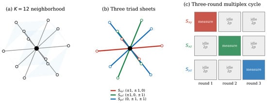
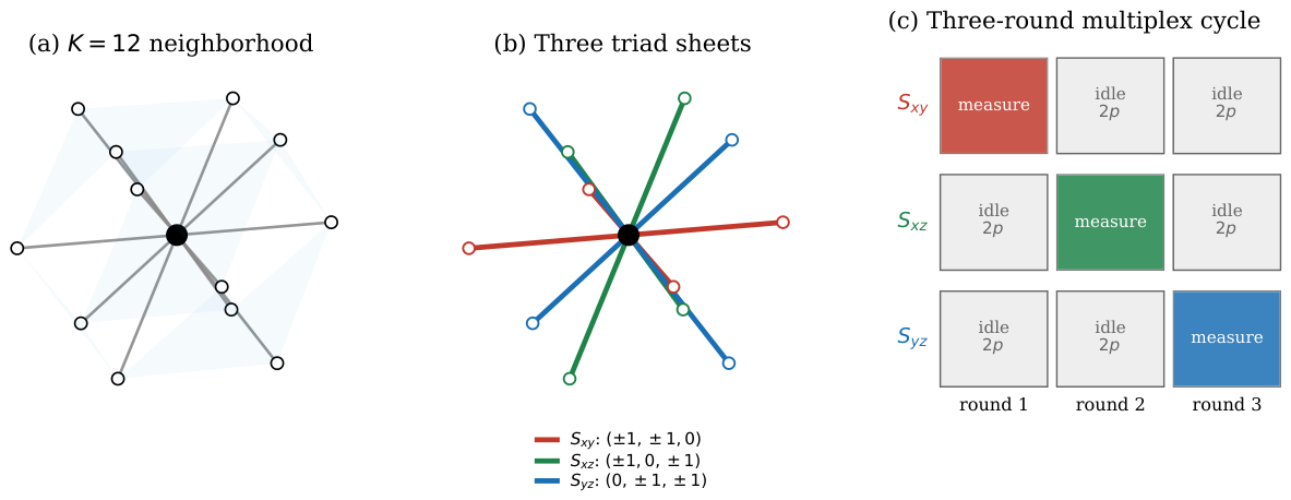
At even L, each sheet holds exactly $L^3$ edges, and every FCC edge lies in exactly one sheet. Each sheet is an edge-disjoint $K=4$ sublattice on the same vertices and octahedral voids. Figure 1 shows the construction.

Figure 1. The three-sheet construction. (a) The twelve nearest-neighbor bonds of an FCC vertex form a cuboctahedron. (b) Those twelve bonds partition into three orthogonal triad sheets of four bonds each. (c) The three-round multiplex cycle: one sheet is measured per sub-round while the other two idle, so each sheet accumulates depolarizing noise at rate $2p$ per cycle. The shared vertex and void ancillas serve all three sheets, which is what reduces the physical-qubit count from $6L^3$ to $4L^3$.

• The single-sheet code.

Fix a sheet S and place a qubit on each of its $L^3$ edges. Z-stabilizers are the weight-4 vertex parity checks over the sheet edges at each FCC vertex; X-stabilizers are the weight-4 checks over the four sheet edges of each octahedral void. This gives a CSS code with parameters $\left[[L^3,2L,L]\right]$, verified directly in Section 6.

• The rotated toric code.

Throughout, “rotated 2D toric code” means the rotated (45°) layout of the toric code [1]: data qubits on the vertices of an $L\times L$ square grid with periodic identification in both directions, one Z-check on each face of one checkerboard color and one X-check on each face of the other, every check of weight four, giving $\left[[L^2,2,L]\right]$. The two logical Z operators are the two non-contractible loops of data qubits that wind once around each periodic direction, and the two logical X operators are the dual loops. At $L=4$, a layer has 16 data qubits, 8 Z-checks and 8 X-checks, and each logical Z has weight 4. In the sheet code, the “square grid” of one layer is the set of $S_{xy}$ edges at fixed z, its vertices are the FCC vertices of that plane, its Z-checks are the vertex checks and its X-checks the void checks restricted to the plane, and the periodic identification is the lattice’s own, which is why only even L is admissible.

• Layer decomposition.

The following is the structural fact this paper rests on. It is stated and proved here so that the argument is self-contained.

Proposition 1.

Each triad sheet decomposes into L disjoint rotated 2D toric codes $\left[[L^2,2,L]\right]$, one per layer of the sheet-orthogonal coordinate.

Proof. 

Take $S=S_{xy}$, whose displacement vectors $(\pm 1,\pm 1,0)$ leave the z coordinate unchanged. Every edge of S therefore lies inside a single plane of constant z, and there are L such planes, each holding $L^3/L=L^2$ edges. Both stabilizer types stay inside one plane. A vertex check uses only the S-edges at that vertex. A void check uses only the four S-edges of the void, and those share the void’s z coordinate. No check couples two planes, so the sheet is L independent codes on disjoint qubit sets, whose joint code space is their tensor product.

Within one plane, the even-parity vertices form a square lattice rotated by 45°. The $(\pm 1,\pm 1,0)$ bonds are its edges. The weight-4 vertex and void checks are its star and plaquette operators on a torus. That is, the rotated toric code $\left[[L^2,2,L]\right]$. Summing over L layers gives $\left[[L^3,2L,L]\right]$.    □

Proposition 1 is confirmed numerically at $L=4$ and $L=6$. The sheet splits into L layers of exactly $L^2$ edges. Every stabilizer sits in one layer. Each layer has $k=2$ with uniform weight-4 checks, and the per-sheet total is $k=2L$.

• Ancilla sharing and multiplexing.

All three sheets occupy one chip: $3L^3$ data qubits in three edge-disjoint groups, plus $L^3/2$ vertex Z-ancillas and $L^3/2$ octahedral X-ancillas. Each ancilla is physically shared by all three sheets, so the total is $4L^3$. Stabilizers are extracted in a three-round cycle whose rounds are the sub-rounds of Section 4, one sheet per sub-round. From any one sheet’s perspective, two sub-rounds in three are idle. If a sub-round takes time t, a sheet’s data qubits idle for $2t$ between successive measurements of their own stabilizers, modeled here as depolarizing noise at rate $2p$ applied once per cycle, additional to gate noise. In Stim, this is DEPOLARIZE1(2p) on the data qubits once per cycle, which is the effective model validated against the explicit schedule in Section 4.

• Combined parameters.

The three sheets are independent code blocks, so the joint code space is the tensor product of the three sheet code spaces, giving $\left[[3L^3,6L,L]\right]$ at periodic boundaries. Writing $p_b$ for the single-sheet block error rate, the three-sheet block error rate is $1-{(1-p_b)}^3$, since the sheets fail independently in the simulated noise model (Section 4). Both quantities are evaluated from simulation in Section Block-Level Failure Probabilities. The text quotes combined parameters because they describe the chip-level resource: one $4L^3$-qubit processor with a shared ancilla set, a shared protocol and a shared decoder. This does not mean that the three sheets form a single code in any stronger sense.

3. Relation to Stacked Toric Codes

The rate figures below invite a comparison that does not survive scrutiny, so the position is stated first.

• Memory performance.

Each sheet is L disjoint rotated toric codes by Proposition 1, and in the simulated noise model the sheets fail independently (Section 4), so the three-sheet code behaves as $3L$ rotated toric codes sharing one ancilla set. Every memory quantity follows: distance L, weight-4 stabilizers, $K=4$ connectivity, and the toric code’s threshold up to the idle penalty quantified in Section 7. The suppression factors of Section 8 are the toric code’s suppression factors.

• Encoding rate.

At $d=4$, the three-sheet code has rate $24/192=12.5\%$. The rotated toric code $\left[\right[16,2,4\left]\right]$ has rate $2/16=12.5\%$. These are equal, and equal at every L: both sit at $2/L^2$ against the rotated surface code’s $1/L^2$. That factor of two comes from periodic boundaries and is available to anyone who accepts wrap-around couplers. It is not a property of the FCC lattice. Any claim that this construction has the highest rate at its distance would be false, and none is made.

• Ancilla sharing.

The three sheets share their ancilla positions. Three separate sheet-code blocks need $6L^3$ physical qubits, $L^3$ data plus $L^3$ ancilla each; the multiplexed chip needs $4L^3$. That is a saving of one third at every L, and it is what this paper quantifies, together with its cost.

• Role of the third dimension.

The same $3L$ toric codes could be laid out separately in two dimensions with identical n, k, and d. The FCC geometry earns its place here for one reason: it places the three sheets on a shared vertex and void set, which is what makes one ancilla set sufficient for three codes.

4. The Multiplex Schedule, Explicitly

The results below rest on a claim about a schedule, so the schedule itself is implemented rather than only its effect.

• Circuit construction.

_fcc_3sheet.py builds all three sheets at once: $3L^3$ data qubits in three edge-disjoint groups, one shared ancilla set of $L^3/2$ vertex and $L^3/2$ octahedral-void ancillas, and $4L^3$ physical qubits in total. Each logical round is three sub-rounds. Sub-round s resets the shared ancillas, extracts sheet s’s weight-4 stabilizers on them, and measures them, while the other two sheets idle. The ancillas are the same physical qubits in every sub-round, which is the construction the paper is about.

• Origin of the factor of two.

Each sheet is active in one sub-round of three and idle in the other two. With a single idle rate $p_{\mathrm{idle}}$ per sub-round, a sheet therefore accumulates $2p_{\mathrm{idle}}$ of idle noise between consecutive measurements of its own stabilizers. The factor of two is a property of the three-round cycle, not a free parameter. Two conventions are fixed here. One sub-round is one unit of time, so a sheet idles for two units between its own extractions. And the effective model applies a single DEPOLARIZE1$\left(2p\right)$ where the explicit circuit applies DEPOLARIZE1$\left(p\right)$ twice; these are not identical channels, since two depolarizing channels of strength p compose to strength $2p-\frac{4}{3}{p}^2$, but the difference is second order in p and is below $0.01\%$ absolute at every rate used here. The validation tables below test the approximation directly rather than relying on that estimate.

• Validation of the effective model.

Simulating three sheets costs three times the qubits and roughly three times the circuit depth per logical round, so for the sweeps, the analysis uses an effective single-sheet circuit that applies DEPOLARIZE1$\left(2p\right)$ to the data qubits once per round. Table 1 compares the two at $L=4$ with $p_{\mathrm{idle}}=p$. At $L=4$, the ratio lies between $0.99$ and $1.05$, that is agreement within $5\%$. Table 2 extends the comparison to $L=6$ across the crossing region with bootstrap confidence intervals on the ratio: there, it lies between $0.99$ and $1.02$, within $2.2\%$, and every $95\%$ interval contains unity. The effective model is therefore an accurate stand-in at the sizes and error rates that matter for the crossings, and it is used for the parameter sweeps. All reported numbers can be reproduced with either circuit.

Table 1. The explicit three-sheet shared-ancilla circuit against the effective single-sheet model, $L=4$, 8000 shots, per-logical error rate. The explicit circuit uses one shared ancilla set and three sub-rounds per round; the effective model applies DEPOLARIZE1$\left(2p\right)$ once per round.

p	Explicit 3-Sheet	Effective $2\mathit{p}$	Ratio
0.002	$1.292\times {10}^{-2}$	$1.228\times {10}^{-2}$	1.05
0.003	$2.494\times {10}^{-2}$	$2.527\times {10}^{-2}$	0.99
0.004	$3.938\times {10}^{-2}$	$3.900\times {10}^{-2}$	1.01
0.005	$5.736\times {10}^{-2}$	$5.759\times {10}^{-2}$	1.00
0.006	$7.591\times {10}^{-2}$	$7.634\times {10}^{-2}$	0.99

Table 2. Explicit three-sheet circuit against the effective model at $L=6$ across the crossing region, 4000 shots each, per-logical error rate. The last column is the $95\%$ bootstrap interval on the ratio from resampling whole shots; every interval contains unity.

p	Explicit 3-Sheet	Effective $2\mathit{p}$	Ratio	$95\%$ CI on Ratio
0.005	$3.09\times {10}^{-2}$	$3.04\times {10}^{-2}$	1.014	$[0.94,1.09]$
0.006	$5.15\times {10}^{-2}$	$5.04\times {10}^{-2}$	1.021	$[0.96,1.09]$
0.007	$7.45\times {10}^{-2}$	$7.31\times {10}^{-2}$	1.020	$[0.97,1.07]$
0.008	$1.051\times {10}^{-1}$	$1.061\times {10}^{-1}$	0.990	$[0.95,1.03]$
0.009	$1.396\times {10}^{-1}$	$1.380\times {10}^{-1}$	1.012	$[0.98,1.04]$
0.010	$1.759\times {10}^{-1}$	$1.721\times {10}^{-1}$	1.022	$[0.99,1.05]$

• Sub-round schedule.

Table 3 sets out one logical round of the explicit circuit, sub-round by sub-round, as implemented in _fcc_3sheet.py. Every two-qubit gate is a CNOT between a data qubit and a shared ancilla, and every data qubit sees at most four per sub-round, two to vertex ancillas and two to void ancillas of its own sheet. No routing is required: each ancilla sits at a lattice vertex or void position that is adjacent to its four data qubits in every sheet.

Table 3. One logical round of the explicit three-sheet circuit. Each sub-round activates one sheet on the single shared ancilla set. Within a sub-round, the Z-checks and X-checks are extracted sequentially; the four CNOTs of each check are scheduled in a fixed order that avoids conflicts, since every ancilla touches four disjoint data qubits. The two idle sheets receive DEPOLARIZE1$\left(p_{\mathrm{idle}}\right)$ once per sub-round.

Sub-Round	Active Sheet	Ancilla Operations on the Shared Set	Idle Sheets
1	$S_{xy}$	reset; Z-checks (4 CNOT/ancilla); measure	$S_{xz}$, $S_{yz}$
		reset; X-checks (H, 4 CNOT/ancilla, H); measure
2	$S_{xz}$	as sub-round 1	$S_{xy}$, $S_{yz}$
3	$S_{yz}$	as sub-round 1	$S_{xy}$, $S_{xz}$

• Scope of the idle channel.

DEPOLARIZE1 on the inactive sheets is a phenomenological stand-in for everything that happens to an idling qubit during another sheet’s extraction. On a neutral-atom platform that would include transport, shelving, and finite-lifetime decay; transport is not modeled explicitly, nor leakage, crosstalk or correlated faults across sheets. The statement that the three sheets fail independently is a property of this noise model and not a claim about hardware, and the distinction is worth making precisely. Code-block independence holds because the three data-qubit sets are disjoint and every stabilizer acts within one sheet. Hardware-level independence would require additionally that the shared ancillas carry no information between sub-rounds, and in the simulated model, they do not: each ancilla is reset before every sub-round, reset is modeled as a fresh preparation followed by an independent X_ERROR, and measurement errors are independent per record. Under those assumptions, an ancilla fault in sheet $S_1$’s sub-round cannot influence the outcome recorded in $S_2$’s sub-round, so no cross-sheet temporal correlation arises. A device with imperfect reset, reset-dependent leakage, measurement crosstalk, shared control lines or correlated transport errors would violate exactly this assumption, and the independence claim would not survive it.

5. Methods

Circuits are built and sampled in Stim 1.15 [6]. For each L, the construction script builds the FCC lattice, identifies the sheet edges, builds the weight-4 vertex and octahedral-void stabilizers, and assembles $H_X$ and $H_Z$ over GF(2). CSS validity $H_X{H}_Z^{\top }=0$ is checked explicitly. Logical-Z observables come from reducing each kernel-of-$H_X$ basis element modulo the row span of $H_Z$.

A memory experiment is L rounds of stabilizer extraction followed by destructive Z-basis measurement. The noise channels are Stim’s standard ones. DEPOLARIZE1$\left(q\right)$ applies one of X, Y, Z to a single qubit, each with probability $q/3$, and identity with probability $1-q$. DEPOLARIZE2$\left(q\right)$ applies one of the fifteen non-identity two-qubit Paulis to a pair, each with probability $q/15$. X_ERROR$\left(q\right)$ applies X with probability q, which on a freshly reset ancilla is a preparation error and immediately before measurement is a readout error. A single parameter p sets every channel, so the noise model has no free relative weights; the idle penalty $2p$ is the one exception and is fixed by the schedule, not tuned. Each round applies three steps in order. First, the multiplex idle penalty DEPOLARIZE1(2p) on all data qubits. Second, Z-stabilizer extraction by CNOT cascade, with DEPOLARIZE2(p) after each CNOT and X_ERROR(p) on ancilla reset and measurement. Third, X-stabilizer extraction by Hadamard-CNOT-Hadamard, with the same noise placement. Detectors are placed on Z-stabilizer outcomes only.

Decoding uses minimum-weight perfect matching (PyMatching 2.3 [7]) on Stim’s detector error model in decompose-errors mode. A logical error on observable i is recorded when the predicted and actual flips disagree. Per-logical error rate is the mean disagreement rate per observable; block error rate is the fraction of shots with at least one disagreement. Sample sizes are 30,000 shots per $(p,L)$ point at $L=4,6$ and 20,000 at $L=8$. Every sampler is seeded from a fixed base seed, with each $(p,L)$ point deriving its own, so the numbers reported here are exactly reproducible from the released code on the same Stim version.

• Crossing extraction.

Thresholds are located from pairwise crossings of the per-logical error rate. For each pair $(L_a,L_b)$, the p grid is scanned in increasing order to find the first interval in which $R_{L_a}\left(p\right)-R_{L_b}\left(p\right)$ changes sign, and the crossing is placed by linear interpolation between the two bracketing points. The p grid is stated with each sweep and is uniform in steps of $0.1\%$ over the crossing region. The quoted threshold is the mean of the three crossings and the quoted uncertainty is their spread. That spread is a finite-size effect and not a statistical error bar, and the two are now separated numerically. Resampling whole shots and re-extracting each crossing 1000 times gives $95\%$ intervals of half-width $0.021$, $0.021$, and $0.034$ percentage points for the $L=4$ vs. 6, 4 vs. 8, and 6 vs. 8 crossings under the three-round cycle, against differences of $0.078$ and $0.074$ percentage points between adjacent crossings. The drift across sizes is therefore three to four times the statistical uncertainty of any single crossing: it is systematic, and it is what the quoted $\pm 0.06\%$ reflects. Throughout, these values are called finite-size crossing estimates. No asymptotic threshold is claimed, and extracting one would require a data-collapse fit over more lattice sizes than the three available here.

• Uncertainties.

Point estimates are per-observable failure rates. Treating $N=\mathrm{shots}\times k$ as the binomial sample size would assume the k logical observables fail independently within a shot, which is not exact, so the analysis instead resamples whole shots with replacement (2000 resamples) and quotes the resulting $95\%$ interval. This preserves any within-shot correlation between observables. The analysis also reports the variance inflation, the ratio of the observed per-shot variance to the value the independence assumption predicts: across all points, it lies between $1.00$ and $1.19$ with median $1.06$, so the naive sample size understates the variance by at most $19\%$, equivalently the standard error by at most $9\%$. Where a point recorded zero failures, the table gives a $95\%$ upper bound from the rule of three rather than a symmetric interval, and elsewhere, Wilson score intervals are used in preference to the normal approximation, which is unreliable at the low-count points.

6. Static Verification

Building the code at $L=4,6,8$ reproduces the predicted parameters exactly, by direct GF(2) computation rather than simulation. Stabilizer ranks satisfy $\mathrm{rank}\left(H_Z\right)=\mathrm{rank}\left(H_X\right)=(L^3-2L)/2$, giving $k=2L$ per sheet and $6L$ across three sheets. Table 4 lists the results, with the qubit saving that motivates the construction. The saving is exactly one third at every size, while the encoding rate $2/L^2$ falls as L grows, from $12.5\%$ at $L=4$ to $3.1\%$ at $L=8$; that decline is the rotated toric code’s and is not affected by the sharing.

Table 4. Sheet code parameters and the ancilla-sharing saving. Physical qubits count data plus ancillas. Three separate blocks need $L^3$ data and $L^3$ ancillas each; the multiplexed chip shares one ancilla set across all three sheets. All constructions verified CSS valid by direct GF(2) computation.

L	1-Sheet	3-Sheet	Physical Qubits		Saving	Rate $6\mathit{L}/3{\mathit{L}}^3$	CSS
	Code	Code	Separate $\mathbf{6} {\mathit{L}}^{\mathbf{3}}$	Shared $\mathbf{4} {\mathit{L}}^{\mathbf{3}}$		(3-Sheet)
4	$\left[\right[64,8,4\left]\right]$	$\left[\right[192,24,4\left]\right]$	384	256	33%	12.5%	yes
6	$\left[\right[216,12,6\left]\right]$	$\left[\right[648,36,6\left]\right]$	1296	864	33%	5.6%	yes
8	$\left[\right[512,16,8\left]\right]$	$\left[\right[1536,48,8\left]\right]$	3072	2048	33%	3.1%	yes

7. Threshold Under the Multiplex Idle Model

The idle penalty is the price of ancilla sharing, and it is quantified here by simulation. Single-sheet operation is compared, where a sheet is measured every sub-round, against three-sheet multiplexing, where it is measured every third sub-round and idles at rate $2p$ in between. The two protocols are identical except for the idle depolarization applied to the data qubits once per cycle, which is 0 and $2p$, respectively.

Both configurations are simulated with the same custom FCC sheet-code circuit used everywhere else in this paper, at the even lattice sizes the construction requires. No surface-code proxy is substituted. Crossings are located from the per-logical error rate, the same metric as Section 8, which is what makes sizes with different $k=2L$ comparable.

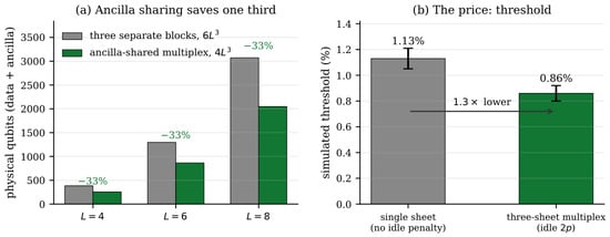
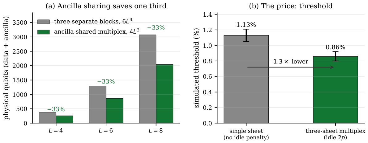
Table 5 lists the pairwise crossings. Single-sheet operation gives $1.13\pm 0.08\%$ and three-sheet multiplexing $0.86\pm 0.06\%$, a reduction of $1.3\times$, that is from $1.13\%$ to $0.86\%$, a $24\%$ relative reduction or $0.27$ percentage points. Figure 2 places this against the qubit saving. Ancilla sharing removes a third of the qubits and gives up somewhat less than a third of the threshold. Whether that is worth taking depends on the operating point: deep below threshold, the suppression is unaffected, as Section 8 shows, while near threshold, the penalty dominates.

Table 5. Pairwise threshold crossings from the full FCC sheet-code circuit, per-logical error rate, 20,000 shots per point. Quoted thresholds are the mean and spread across the three crossings.

Crossing	Single Sheet	Three-Sheet Multiplex
$L=4$ vs. $L=6$	1.233%	0.931%
$L=4$ vs. $L=8$	1.136%	0.855%
$L=6$ vs. $L=8$	1.026%	0.787%
estimate	$1.13\pm 0.08\%$	$0.86\pm 0.06\%$

Figure 2. The trade quantified. (a) Ancilla sharing needs $4L^3$ physical qubits against $6L^3$ for three separate blocks, a saving of one third at every L. (b) The simulated circuit-level threshold falls from $1.13\%$ to $0.86\%$ under the multiplex idle penalty, a factor of $1.3$. Both are obtained with the full FCC sheet-code circuit; error bars are the spread across the three pairwise crossings.

• Relation to a surface-code proxy.

One sheet layer is a rotated toric code with $k=2$ and periodic boundaries. It is tempting to substitute a rotated surface code with $k=1$ and open boundaries, whose memory circuit is built into standard tooling. Both were simulated, and the substitution is not recommended: the proxy and the actual circuit differ in noise placement and in logical count, and they do not give the same crossing. All thresholds reported here come from the actual circuit.

7.1. Sensitivity to the Idle Model

The three-round cycle fixes $r\equiv p_{\mathrm{idle}}/p_{2q}=2$, but the identification of the idle rate with the two-qubit gate rate is a modeling choice. The ratio r is therefore swept and the crossing estimate reported as a function of it, so that the trade-off can be read off for whatever ratio a platform actually delivers. Table 6 gives the result.

Table 6. Threshold against the idle-to-gate noise ratio $r=p_{\mathrm{idle}}/p_{2q}$, from the pairwise crossings at $L=4,6,8$. $r=0$ is single-sheet operation, $r=2$ the three-round cycle used throughout. All three crossings bracket at every ratio. Over the sampled values, the finite-size crossing estimates decrease monotonically, with no abrupt change; four points do not establish the functional form, but they show the reported penalty is not an artifact of fixing $r=2$.

r	Crossings (%)	Threshold	Penalty vs. $\mathit{r}=0$
0	1.233, 1.136, 1.026	$1.13\pm 0.08\%$	$1.00\times$
1	1.072, 0.970, 0.873	$0.97\pm 0.08\%$	$1.17\times$
2	0.931, 0.855, 0.787	$0.86\pm 0.06\%$	$1.32\times$
4	0.765, 0.709, 0.641	$0.71\pm 0.05\%$	$1.59\times$

Doubling the idle ratio from 1 to 2 costs $0.11$ percentage points and doubling again from 2 to 4 costs $0.15$; within this limited data set, the penalty grows more slowly than the idle rate. A platform whose idle decoherence per sub-round equals its two-qubit gate error rate, that is $r=1$ rather than the $r=2$ of the three-round cycle, would see a crossing estimate near $0.97\%$ rather than $0.86\%$.

7.2. Both Pauli Sectors

The circuit of Section 5 places detectors on Z-stabilizer outcomes and reads out in the Z basis, which characterizes the Z memory. To check that the threshold is not specific to that sector, a dual circuit was built: data qubits initialized and read out in the X basis, detectors on the X-stabilizer outcomes, and the logical-X basis as observables. Table 7 compares the two.

Table 7. Threshold in both Pauli sectors under the three-round cycle. The bands overlap, so the reported threshold is a memory threshold rather than a property of one sector. The X sector is marginally weaker, as expected when Z-stabilizers are extracted first in each sub-round.

Sector	Crossings (%)	Threshold
Z memory	0.931, 0.855, 0.787	$0.86\pm 0.06\%$
X memory	0.844, 0.773, 0.717	$0.78\pm 0.05\%$

8. Sub-Threshold Distance Scaling

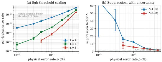
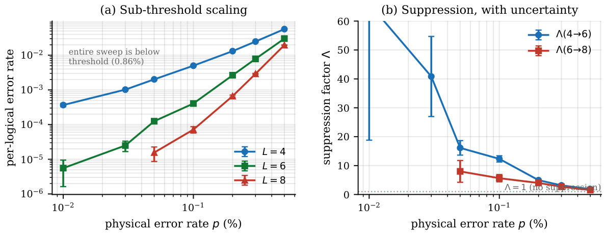
Table 8 reports per-logical error rates for the full three-sheet circuit under the idle penalty, and Table 9 the corresponding suppression factors. Figure 3 plots both.

Table 8. Per-logical error rate for the three-sheet multiplexed code under the DEPOLARIZE1(2p) idle penalty. Brackets give the $95\%$ shot-level bootstrap interval in units of the leading factor. 30,000 shots at $L=4,6$ and 20,000 at $L=8$. Entries shown as a bound observed no failures; these are the $L=8$ points at $p={10}^{-4}$ and $p=3\times {10}^{-4}$, and they carry a rule-of-three $95\%$ upper limit rather than an interval.

p	$\mathit{L}=4$	$\mathit{L}=6$	$\mathit{L}=8$
0.0001	$3.67\times {10}^{-4}$ [2.87, 4.46]	$5.6\times {10}^{-6}$ [0, 13.9]	<$9.4\times {10}^{-6}$
0.0003	$1.02\times {10}^{-3}$ [8.96, 11.5]	$2.50\times {10}^{-5}$ [1.11, 4.17]	<$9.4\times {10}^{-6}$
0.0005	$2.02\times {10}^{-3}$ [1.83, 2.21]	$1.25\times {10}^{-4}$ [0.92, 1.64]	$1.56\times {10}^{-5}$ [0.31, 3.13]
0.001	$5.00\times {10}^{-3}$ [4.72, 5.30]	$4.06\times {10}^{-4}$ [3.39, 4.72]	$7.19\times {10}^{-5}$ [4.37, 10.0]
0.002	$1.31\times {10}^{-2}$ [1.27, 1.36]	$2.65\times {10}^{-3}$ [2.47, 2.82]	$6.63\times {10}^{-4}$ [5.78, 7.53]
0.003	$2.48\times {10}^{-2}$ [2.42, 2.55]	$7.85\times {10}^{-3}$ [7.55, 8.15]	$2.91\times {10}^{-3}$ [2.72, 3.11]
0.005	$5.67\times {10}^{-2}$ [5.57, 5.77]	$3.02\times {10}^{-2}$ [2.96, 3.08]	$1.96\times {10}^{-2}$ [1.90, 2.01]

Table 9. Suppression factor $\mathsf{\Lambda }(L\to L+2)$, with uncertainty propagated from the shot-level bootstrap. The $p={10}^{-3}$ row corresponds to currently demonstrated trapped-ion two-qubit gate fidelities and is the row with adequate statistics at every size. Values at lower p are limited by the shot floor, and n/a marks a ratio whose denominator observed no errors.

p	$\mathbf{\Lambda }(4\to 6)$	$\mathbf{\Lambda }(6\to 8)$
0.0003	$40.8\pm 13.8$	n/a
0.0005	$16.1\pm 2.5$	$8.0\pm 3.7$
0.001	$12.3\pm 1.1$	$5.6\pm 1.2$
0.002	$5.0\pm 0.2$	$4.0\pm 0.3$
0.003	$3.2\pm 0.1$	$2.7\pm 0.1$
0.005	$1.9\pm 0.1$	$1.5\pm 0.1$

Figure 3. Distance scaling of the three-sheet multiplexed code under the idle penalty. (a) Per-logical error rate against physical depolarizing rate at $L=4,6,8$. Error bars here are binomial standard errors computed from the plotted rate and the shot count; the intervals quoted in Table 8 are shot-level bootstrap intervals, which are asymmetric at the low-count points and are the ones to read for those entries. The sweep reaches $0.5\%$, well below the $0.86\%$ threshold of Table 5, so every point shown is sub-threshold and no crossing appears in this range. (b) Suppression factors with propagated uncertainty. The large values at low p carry correspondingly large error bars and are limited by the shot floor. The three curves in (a) converge toward the right and the suppression factors in (b) fall toward 1 for the same reason: as p approaches the finite-size crossing near $0.86\%$, increasing L stops helping, because above threshold, a larger code has more places for an uncorrectable error to occur. The convergence is the threshold being approached from below, not a failure of the code.

At $p={10}^{-3}$, the per-logical error rate is $(5.00\pm 0.14)\times {10}^{-3}$ at $L=4$, $(4.06\pm 0.34)\times {10}^{-4}$ at $L=6$, and $(7.19\pm 1.50)\times {10}^{-5}$ at $L=8$. The suppression factors are $\mathsf{\Lambda }(4\to 6)=12.3\pm 1.1$ and $\mathsf{\Lambda }(6\to 8)=5.6\pm 1.2$. The rate falls by a factor of $12.3$ from $L=4$ to $L=6$ and $5.6$ from $L=6$ to $L=8$; the second factor is smaller because $L=8$ at this rate is close to the shot floor, not because suppression has weakened. Suppression survives both the ancilla sharing and the idle penalty. That is the result this section is for.

• Shot-floor limited points.

At $p={10}^{-4}$, the $L=6$ estimate rests on two observed logical errors across 30,000 shots and twelve observables, so its uncertainty is $70\%$. The $L=8$ points at $p={10}^{-4}$ and $p=3\times {10}^{-4}$ recorded zero errors in 20,000 shots and are quoted only as upper bounds. The largest suppression factor in Table 9 is $\mathsf{\Lambda }(4\to 6)=40.8\pm 13.9$ at $p=3\times {10}^{-4}$. Its $34\%$ uncertainty means it should not be read as a precise value. The $p={10}^{-3}$ row has adequate statistics at every size, and that is the row the text quotes.

• Comparison with hardware.

Suppression factors measured deep below threshold in simulation are not comparable to those measured on hardware near threshold. A surface-code simulation at $p={10}^{-3}$ would also show large $\mathsf{\Lambda }$. The hardware value $\mathsf{\Lambda }\approx 2.14$ reported for Willow [8] was measured near threshold, on a single logical qubit. The sheet code decomposes into toric codes, so the values here are the toric code’s. No claim of advantage is therefore made over the surface code from these numbers. What they establish is narrower and is what is intended: suppression survives ancilla sharing and the idle penalty, on a memory carrying 24 to 48 logical qubits.

Block-Level Failure Probabilities

The per-logical error rate is the natural quantity for comparing sizes, but it understates what a chip-level user experiences. With $k=2L$ logical observables per sheet and three sheets, a low per-logical rate coexists with a substantial probability that at least one logical qubit has failed. Table 10 reports both. The block rate is the fraction of shots in which any of a sheet’s $2L$ observables failed, taken directly from the per-shot data; the three-sheet figure is $1-{(1-P_{\mathrm{block}})}^3$, which assumes the sheets fail independently, a property of the simulated model stated in Section 4.

Table 10. Per-logical rate against block-level failure under the three-round cycle. “Block” is the probability that at least one of a sheet’s $2L$ logical observables fails in a memory experiment of L rounds; “any of 3” is the probability that at least one of the three sheets’ blocks fails. At $L=6$, the 36-logical instance discussed in Section 10, a per-logical rate of $0.05\%$ at $p={10}^{-3}$ corresponds to a $1.6\%$ probability per experiment that some logical qubit has failed.

L	p	Per-Logical	Block ($2\mathit{L}$ obs.)	Any of 3 Sheets
4	0.001	$5.7\times {10}^{-3}$	$4.2\times {10}^{-2}$	$1.21\times {10}^{-1}$
4	0.003	$2.5\times {10}^{-2}$	$1.74\times {10}^{-1}$	$4.36\times {10}^{-1}$
4	0.005	$5.6\times {10}^{-2}$	$3.40\times {10}^{-1}$	$7.13\times {10}^{-1}$
6	0.001	$5.0\times {10}^{-4}$	$5.5\times {10}^{-3}$	$1.64\times {10}^{-2}$
6	0.003	$8.2\times {10}^{-3}$	$9.0\times {10}^{-2}$	$2.46\times {10}^{-1}$
6	0.005	$3.0\times {10}^{-2}$	$2.89\times {10}^{-1}$	$6.41\times {10}^{-1}$
8	0.001	<$5\times {10}^{-5}$	$5\times {10}^{-4}$	$1.5\times {10}^{-3}$
8	0.003	$3.1\times {10}^{-3}$	$4.5\times {10}^{-2}$	$1.29\times {10}^{-1}$
8	0.005	$1.9\times {10}^{-2}$	$2.49\times {10}^{-1}$	$5.76\times {10}^{-1}$

The block figures make the resource trade concrete in a way the per-logical figures do not. At $p={10}^{-3}$, the $L=6$ chip loses at least one of its 36 logical qubits in about one experiment in sixty; at $p=3\times {10}^{-3}$, in one in four. Multiplying the per-logical rate by the 36 observables would give $1.8\%$ at $p={10}^{-3}$, against the $1.6\%$ actually observed. The naive product is close at this rate because coincident failures are rare, but the two separate as p grows: at $p=3\times {10}^{-3}$, the product gives $30\%$ against $25\%$ observed, and at $p=5\times {10}^{-3}$, it exceeds unity while the observed figure is $64\%$. It is the observed figure that a user of the chip would need. They also sharpen the comparison with three separate blocks, which have the same block-failure probabilities at $r=0$ but pay $6L^3$ qubits for them.

9. Rate and Distance at $\mathit{d}=\mathbf{4}$

Table 11 compares at $d=4$. The essential row is the rotated toric code, which is often omitted in favor of the rotated surface code and which the three-sheet construction matches exactly.

Table 11. Comparison at distance $d=4$, counting data qubits only. The three-sheet code and the rotated toric code have identical rate, as the layer decomposition requires. The factor of two over the rotated surface code is the periodic-boundary factor. The smallest bivariate-bicycle instances are at $d=6$ and $d=12$, so no $d=4$ comparison is possible.

Code	n	k	Rate	K	Note
Rotated surface $\left[\right[16,1,4\left]\right]$	16	1	6.3%	4	open boundaries
Rotated 2D toric $\left[\right[16,2,4\left]\right]$	16	2	12.5%	4	periodic
3D toric (cubic)	192	3	1.6%	6
FCC 3-sheet (this work)	192	24	12.5%	4	=12 rotated toric codes

Per-logical fidelity, meaning one minus the per-logical error rate, and encoding rate, the number of logical qubits per data qubit, trade against each other: a code with more logical qubits per physical qubit at fixed distance generally has a higher per-logical error rate at fixed p. At $p={10}^{-3}$, a single $\left[\right[16,1,4\left]\right]$ rotated surface code block has a per-logical error rate near $5\times {10}^{-4}$, against $5.00\times {10}^{-3}$ here (Table 8). The surface code has the lower per-logical error rate at $d=4$. On the data-only axis of this table, the three-sheet code and the rotated toric code are equal, at 8 data qubits per logical qubit, and both beat the rotated surface code’s 16 by the periodic-boundary factor. Neither figure includes ancillas, so the ancilla sharing that this paper is about does not appear here at all: it shows up in the physical counts of Table 4, where the three-sheet chip needs $4L^3$ against $6L^3$ for three separate blocks. Nothing in either comparison is intrinsic to the FCC lattice.

10. Qubit-Count Context and Implementation Requirements

The three-sheet code at $L=4$ needs 256 physical qubits at $K=4$, and at $L=6$ needs 864. Neutral-atom platforms are the closest match to the protocol’s requirements among the platforms listed, on qubit count and on reconfigurable connectivity, but that is a statement about counts and coupling geometry rather than a feasibility claim. Optical-tweezer rearrangement lets one ancilla set be brought to each data group in turn, which is the mechanism the three-round cycle assumes; that suitability is what the sections below qualify.

Table 12 lists current platform qubit counts against the requirements of the two smallest instances. The smallest instance with a substantial logical count is $L=6$: $\left[\right[648,36,6\left]\right]$ on 864 physical qubits, a number within the nominal atom count of Atom Computing’s Phoenix processor [9]. A matching count is a precondition, not a demonstration of feasibility; the requirements a device would additionally have to meet are listed with the table, and none is modeled here. Running $L=4$ first and then $L=6$ on the same processor would give a measurement of $\mathsf{\Lambda }$ on a multi-logical memory, which the author is not aware of having been reported on any platform. The nearest prior multi-logical demonstration encoded 24 logical qubits with the distance-2 $\left[\right[4,2,2\left]\right]$ code on a 256-atom processor [9], which is error detection rather than correction. The ancilla saving is what brings $L=6$ inside the machine at all: three separate blocks would need 1296 physical qubits and would not fit.

Table 12. Production hardware as of May 2026 against the three-sheet requirement. This is a raw qubit-count comparison only, and the section is titled accordingly. Counts are as stated by each vendor as of May 2026 and are subject to change; only the Atom Computing figure rests on a peer-reviewed source, and the others are vendor announcements or roadmaps rather than demonstrated device sizes. A device matching the count is not thereby able to run the protocol: that additionally requires the FCC connectivity to be realizable in the trap geometry, periodic boundaries or the planar variant, mid-circuit measurement and reset on the shared ancillas, transport or coupling to pair one ancilla set with three data groups in sequence, and gate fidelity, atom loss, and timing within the budgets implied by Section 7.1. None of these is analyzed here. The entries below therefore report qubit count alone: “count only” means the device has enough qubits and nothing further is claimed, and “marginal” means the count matches with no headroom.

Platform	Qubits	$\mathit{L}=4$ (256q)	$\mathit{L}=6$ (864q)	Source
IBM Heron r3	156	no	no	vendor roadmap
IBM Nighthawk	120	no	no	vendor roadmap
Quantinuum Helios	98	no	no	vendor announcement
Atom Computing Phoenix	1180+	count only	count only	Ref. [9]
Pasqal Orion	1024	count only	count only	vendor announcement
QuEra Gemini	256	marginal	no	vendor announcement

A Limited d = 4 Circuit Comparison Against the Surface Code

This comparison is illustrative and not a performance ranking. The baseline is an open-boundary rotated surface code with one logical qubit, different boundary conditions from the periodic toric layers of the sheet code, and no multiplexing idle penalty, so the two are matched in distance and noise parameter only. The per-logical comparison value in Section 9 comes from surface_code_baseline.py and is stated here in full so it can be reproduced or disputed. The circuit is Stim’s rotated planar memory at $d=4$, $\left[\right[16,1,4\left]\right]$, run for d rounds with the same uniform noise parameter p applied to the same channel types as the paper’s own circuit: DEPOLARIZE2 on every two-qubit gate, X_ERROR on ancilla reset and measurement and on the final data readout, and no idle penalty. Decoding is MWPM on the decomposed detector error model. With $\mathrm{30,000}$ shots at $p={10}^{-3}$, the per-logical error rate is $4.3\times {10}^{-4}$ with a $95\%$ bootstrap interval of $[2.6,6.3]\times {10}^{-4}$; a ${10}^6$-shot run gives $4.8\times {10}^{-4}$. The surface-code circuit has one logical observable, so the sample-size question of Section 5 does not arise for it.

11. Limitations

• Idle noise model.

The $2p$ per-cycle idle rate is a model choice, not a measurement. Actual idle decoherence during neutral-atom rearrangement and shelving is a separate experimental question, and the threshold cost reported here scales with it.

• Scope of the memory result.

As Proposition 1 shows, the sheets are independent and each decomposes into toric layers. Nothing in the distance-scaling data is specific to the FCC lattice beyond the ancilla sharing and the idle penalty.

• No logical operations.

This paper concerns memory only. Operations between sheets would couple the codes non-trivially and require treating the joint Hilbert space as one object; they are not addressed here.

• Three lattice sizes.

Every crossing estimate in this paper rests on $L=4,6,8$. Three sizes are enough to bracket a crossing but not to separate the crossing location from finite-size drift by fitting: the drift across the three pairwise crossings is systematic and about three to four times the statistical uncertainty of any single crossing (Section 5), and no data-collapse fit is attempted, so no asymptotic threshold or critical exponent is extracted. $L=4$ is also below the size at which the d-round memory experiment is fault-tolerant in the usual sense. Adding $L=10$ would require roughly three times the shots at the low-p end to reach comparable statistics and is left to future work.

• Lattice sizes and decoder.

Simulations run to $L=8$. MWPM is a standard choice for weight-4 surface-code-like stabilizers, but stabilizer weight alone does not establish decoder optimality under circuit-level correlated noise, and no optimality claim is made. The exact layer decomposition does mean that no cross-layer correlations exist for a decoder to exploit. Within a layer, a correlated or belief-propagation assisted decoder could still improve on these numbers, which would raise the reported thresholds rather than lower them. Stim’s decompose_errors option is enabled throughout. It splits any error mechanism that flips more than two detectors into graph-like components, which is an approximation when such mechanisms exist. In these circuits none do. Building the detector error model with decompose_errors=False and counting mechanisms by the number of detectors they flip gives zero with more than two, at every size and in every circuit variant used here: the Z-memory at $r=0$ and $r=2$, the X-memory, and the explicit three-sheet circuit. The reason is structural: detectors are placed on one stabilizer type, every check has weight four, and every data qubit lies in exactly two checks of that type, so no single Pauli fault can flip more than two detectors. Decoding the same $\mathrm{20,000}$ shots at $L=4$, $p=0.8\%$ with the raw and the decomposed model gives identical predictions on every shot. The decomposition therefore has no effect on any reported number, and no correlated-fault approximation is being made.

12. Conclusions

The three triad sheets of the FCC lattice share their vertex and void ancilla positions. Measuring them in a three-round time-multiplexed cycle on one shared ancilla set reduces the physical-qubit count of three sheet-code blocks from $6L^3$ to $4L^3$, a saving of exactly one third at every even L. That schedule is implemented as an explicit circuit and shown to agree with the effective single-sheet model used for the sweeps to within $5\%$ at $L=4$ and $2.2\%$ at $L=6$.

The cost is a finite-size crossing estimate of the circuit-level threshold that falls from $1.13\pm 0.08\%$ to $0.86\pm 0.06\%$ under the three-round cycle: a factor of $1.3$, or $0.27$ percentage points, a $24\%$ relative reduction. Across the sampled idle-to-gate ratios $r=0,1,2,4$, the estimates decrease monotonically, from $1.13\%$ to $0.71\%$, so the penalty is not an artifact of one modeling choice. The X-basis memory gives $0.78\pm 0.05\%$, overlapping the Z value. The spreads quoted on these estimates are dominated by systematic drift across the three lattice sizes rather than by statistical error, which is three to four times smaller.

Sub-threshold suppression survives the sharing, at $\mathsf{\Lambda }(4\to 6)=12.3\pm 1.1$ and $\mathsf{\Lambda }(6\to 8)=5.6\pm 1.2$ at $p={10}^{-3}$. These are the suppression factors of the underlying rotated toric codes, and the memory is not claimed to be new: each sheet is exactly L such codes, its encoding rate equals the rotated toric code’s at every distance, and the surface-code comparison in Section 9 is a limited $d=4$ circuit comparison and not a performance ranking. At the chip level, block failure probabilities grow with the logical count: at $L=6$ and $p={10}^{-3}$, the 36-logical instance loses at least one logical qubit in about one experiment in sixty.

The detector error model of every circuit used here is graph-like, with no error mechanism flipping more than two detectors, so the matching decoder makes no correlated-fault approximation. The independence of the three sheets holds in the simulated model because every shared ancilla is reset between sub-rounds and reset, measurement and gate faults are independent; a device with imperfect reset or measurement crosstalk would not inherit it.

Two directions would sharpen the result. Adding a fourth lattice size would let the crossing be separated from the finite-size drift by fitting rather than by bracketing, which is what the present three sizes cannot do. And measuring the idle decoherence a given platform actually delivers would replace the modeling choice $r=2$ with a device number, turning Table 6 from a sensitivity sweep into a prediction for that platform.

The $L=6$ instance, $\left[\right[648,36,6\left]\right]$, needs 864 physical qubits. That number lies within the nominal atom count of current neutral-atom processors, but a matching count is a precondition and not a demonstration: realizing the FCC connectivity in a trap geometry, the wrap-around couplers the periodic construction needs, mid-circuit reset on the shared ancillas, atom loss, leakage, crosstalk and correlated transport errors are all unmodeled here, and no implementability claim is made beyond the count.

References

- Fowler, A.G.; Mariantoni, M.; Martinis, J.M.; Cleland, A.N. Surface codes: Towards practical large-scale quantum computation. Phys. Rev. A 2012, 86, 032324. [Google Scholar] [CrossRef] [Scilit]
- Bravyi, S.; Cross, A.W.; Gambetta, J.M.; Maslov, D.; Rall, P.; Yoder, T.J. High-threshold and low-overhead fault-tolerant quantum memory. Nature 2024, 627, 778. [Google Scholar] [CrossRef] [Scilit]
- Kulkarni, R. A 67%-Rate CSS Code on the FCC Lattice: [[192,130,3]] from Weight-12 Stabilizers. arXiv 2026, arXiv:2603.20294. [Google Scholar] [CrossRef] [Scilit]
- Hu, X.; Sarma, S.D. Gate errors in solid-state quantum-computer architectures. Phys. Rev. A 2002, 66, 012312. [Google Scholar] [CrossRef] [Scilit][Green Version]
- Zhang, W.; Dobrovitski, V.V.; Al-Hassanieh, K.A.; Dagotto, E.; Harmon, B.N. Hyperfine interaction induced decoherence of electron spins in quantum dots. Phys. Rev. B 2006, 74, 205313. [Google Scholar] [CrossRef] [Scilit]
- Gidney, C. Stim: A fast stabilizer circuit simulator. Quantum 2021, 5, 497. [Google Scholar] [CrossRef] [Scilit]
- Higgott, O. PyMatching: A Python Package for Decoding Quantum Codes with Minimum-Weight Perfect Matching. ACM Trans. Quantum Comput. 2022, 3, 16. [Google Scholar] [CrossRef] [Scilit]
- Google Quantum AI and Collaborators. Quantum error correction below the surface code threshold. Nature 2025, 638, 920, Correction in Nature 2026, 653, E5. https://doi.org/10.1038/s41586-026-10559-8. [Google Scholar] [CrossRef] [Scilit]
- Reichardt, B.W.; Paetznick, A.; Aasen, D.; Basov, I.; Bello-Rivas, J.M.; Bonderson, P.; Chao, R.; van Dam, W.; Hastings, M.B.; Paz, A.; et al. Logical computation demonstrated with a neutral atom quantum processor. arXiv 2024, arXiv:2411.11822. [Google Scholar] [CrossRef] [Scilit]
Disclaimer/Publisher’s Note: The statements, opinions and data contained in all publications are solely those of the individual author(s) and contributor(s) and not of MDPI and/or the editor(s). MDPI and/or the editor(s) disclaim responsibility for any injury to people or property resulting from any ideas, methods, instructions or products referred to in the content. |
© 2026 by the author. Licensee MDPI, Basel, Switzerland. This article is an open access article distributed under the terms and conditions of the Creative Commons Attribution (CC BY) license.