


Abstract
Restricting the FCC lattice code to a single triad sheet gives the sheet code, with uniform weight-4 stabilizers and active connectivity. This code is isomorphic to L disjoint rotated 2D toric codes, so its memory is the toric code’s, and no density advantage is claimed. The contribution is a logical interconnect: native fault-tolerant joint Pauli measurement between selected logical qubits in independently encoded, co-located code blocks, with no dedicated routing region. Its natural use is entanglement generation and parity measurement between such blocks, since the and merges characterized here are exactly the two measurements a logical Bell measurement requires. Every FCC triangle has one edge in each triad sheet, so products of triangle measurements implement joint Pauli measurements across sheets while the merged code retains . Finite-size crossing estimates under circuit-level depolarizing noise at are for the -merge, with planar boundaries, and for the -merge. The value of the primitive is that, for the pairs it reaches, it needs no routing region. Surface-code surgery merges only adjacent patches, so joining arbitrary pairs costs a reservation of roughly tiles per logical qubit; within the directly reachable set, the sheet architecture avoids that reservation, using physical qubits per logical, against for a bussed toric array. That set is structured and limited: at the verified sizes of , each basis logical reaches L partners in one other sheet, giving directly measurable pairs, corresponding to about of all logical pairs, and the same pattern is conjectured for general even L values. Three limits are stated rather than deferred: only the joint measurements are fault-tolerant primitives, the composed three-sheet CNOT being verified but not yet fault-tolerantly characterized; all thresholds are finite-size crossings at three lattice sizes, not asymptotic values; and pairs outside the reachable set would need routing as in any other architecture.
1. Introduction
Two families of quantum error correcting codes currently dominate the discussion of near-term fault-tolerant quantum computing. The surface code [1,2] pairs planar hardware compatibility with mature fault-tolerant protocols, including lattice surgery [3,4] for logical gates within a single 2D substrate. The bivariate bicycle (BB) code family [5] achieves an order-of-magnitude rate advantage over the surface code at the cost of connectivity and a small number of long-range couplers. The BB family’s inter-block logical gates, which move logical qubits between distinct code blocks, remain an active research problem [6].
This paper introduces a third option, occupying a niche that Section 8 argues is not filled by either family: a CSS code at connectivity (matching the surface code) with native inter-sheet joint Pauli measurements between co-located CSS code blocks. A fault-tolerant primitive that the surface code provides only within a single patch’s lattice surgery zone is a different design point than surface-code lattice surgery (which operates within a single substrate) and bivariate bicycle codes (which target inter-block gates between physically separated modules and where modular logical operation protocols are an area of active architectural development). Full FT logical CNOT composition between sheets is a synthesis of two such joint Pauli primitives, verified at the truth-table level but identified as not yet fault-tolerantly characterized in this work (Section 10); the primary characterized contribution is the joint Pauli primitive itself. The construction has two interlocking ingredients.
The interconnect problem. Any modular fault-tolerant architecture needs a way to entangle or parity-check logical qubits held in different code blocks. In a planar layout, that is a routing problem: the two blocks must be brought adjacent to one another, or a reserved region must carry the operation between them, and the reservation is paid whether or not it is in use. What this paper offers is a logical interconnect in which a structured set of cross-block pairs is joinable directly because the geometry has already placed them within reach of a single weight-3 measurement. The interconnect is sparse, reaching L partners per logical in one other block at the verified sizes, but for those pairs, it provides the two merges a fault-tolerant Bell measurement between independently encoded blocks, with no routing cost. That is the capability to keep in view through the construction that follows: not a new memory but a way to wire logical memories together.
The FCC sheet code. Restricting the FCC lattice code [7] to a single triad sheet (one of three orthogonal sublattices in FCC) removes every weight-3 logical operator of that code and yields a CSS code with parameters of at even L values. Theorem 2 shows this code is isomorphic to L disjoint rotated 2D toric codes. The consequence follows directly: the sheet code’s memory is the toric code’s memory, and no advantage is claimed there. Three sheets on a shared FCC substrate encode logical qubits at a distance of L on data qubits, which is the same qubits-per-logical count as separate rotated toric codes.
Cross-sheet triangle surgery. Every FCC triangle has one edge in each of the three triad sheets. Weight-3 Pauli measurements on FCC triangles couple data qubits across sheets, providing a natural primitive for inter-sheet logical operations. Triangle products are shown to implement joint Pauli measurements between logical qubits in different sheets, with the merged code preserving a distance of .
Value of the combination. Because the memory is the toric code’s, the case for the architecture rests entirely on the primitive, as quantified in Section 8.4 rather than left qualitative. A rotated toric array merges only adjacent patches, so an architecture joining arbitrary pairs reserves routing space at roughly tiles per logical qubit [4]. For the pairs a triangle primitive reaches directly, the sheet architecture needs no such reservation, and at a matched distance, it uses physical qubits per logical qubit, against for a bussed toric array. At the verified sizes of , that set is basis pairs, corresponding to about of all logical pairs, with each basis logical reaching L partners in one other sheet (Proposition 3); the pattern is conjectured, not proven, for general L values. For other pairs, routing is needed as elsewhere, and no advantage is claimed.
The two ingredients work in tandem: the sheet code provides toric-code storage at ; the triangle surgery primitive provides fault-tolerant inter-sheet joint Pauli measurements at the same envelope. The result fills a gap that neither surface code nor bivariate bicycle codes address: planar connectivity with inter-sheet joint Pauli measurements as a native primitive. Composing these primitives into full FT logical gates (Clifford circuits, magic-state distillation, etc.) requires the further protocol or hardware refinements identified in Section 10.
Summary of results. (i) Sheet code with parameters on a torus, on a plane, uniform weight-4 stabilizers, and data-qubit connectivity (Section 2); (ii) three-sheet hardware architecture via time-multiplexed syndrome extraction (Section 3); (iii) triangle algebra spanning of the cross-sheet Z-logicals, with a two-sheet basis (Section 4); (iv) fault-tolerant surgery protocol with verification and gate overhead (Section 5); (v) distance preservation under merge for both Z- and X-sides (Section 6); (vi) threshold simulation via custom Stim at , giving (toric) and (boundary-aware planar) (Section 7); (vii) comparison with state of the art (Section 8); (viii) CSS-dual XX-merge primitive demonstrated at on the toric variant, with the merged sheet pair pinned across sizes, giving (Section 9.3); (ix) three-sheet Horsman CNOT logical truth table verified at but not yet fault-tolerantly characterized (Section 10).
Claim status matrix. To make the epistemic status of each claim transparent up front, we propose the following:
Table 1 summarizes the epistemic status of every claim made in this paper.
Table 1.
Epistemic status of each claim made in this paper.
2. The FCC Sheet Code
2.1. The Triad Decomposition
Coordinates and boundary conditions. Sites are indexed by integer coordinates , with and all arithmetic taken modulo L, so the lattice is a 3-torus. FCC sites are those with even, giving vertices. The parity condition closes under the periodic identification only when L is even: for odd L values, a translation by L along one axis flips , so the even-parity sublattice does not close, and the construction fails. Every lattice size in this paper is therefore even. The planar variant of Section 9.2 drops the wrap-around identification at the usual cost in k.
The FCC lattice has nearest-neighbor vectors, partitioning into three orthogonal sheets of four:
Each FCC edge belongs to exactly one sheet, since the three displacement classes are disjoint. At even lattice sizes (L) each sheet contains exactly edges, and restricted to a single sheet, each FCC vertex has incident edges. Both counts are verified directly at and : vertices, edges in each of the three sheets, and a uniform per-sheet vertex degree of 4.
2.2. The Sheet-Code Stabilizers
Definition 1
(FCC sheet code). Fix one triad sheet (S; say, ). Place one physical qubit on each edge in S ( qubits). The stabilizers are:
- Z-stabilizers: For each vertex (v), apply Z to the four edges of incidents S to v.
- X-stabilizers: For each octahedral void (o), apply X to the four edges of S connecting the six vertices surrounding o.
Both stabilizer types have a uniform weight of 4. The CSS condition () over holds because every overlap is either empty or of size two. Fix a vertex (v) and an octahedral void (o) and consider , the number of sheet-S edges incident to v that also lie on the octahedron around o. The four sheet-S edges of that octahedron form a four-cycle through the four surrounding vertices lying in the plane of S; the remaining two surrounding vertices are apexes and carry no sheet-S edge of the octahedron. If v is not one of the six surrounding vertices, the overlap is 0; if v is an apex, it is, again, 0, and if v is one of the four in-plane vertices, exactly two edges of the four-cycle meet it, so the overlap is 2. The overlap is therefore always even, and the two stabilizer groups commute. Direct computation confirms it: at and , the only overlap values occurring between any X-stabilizer and any Z-stabilizer are 0 and 2.
2.3. Code Parameters
Theorem 1
(Sheet code parameters). At even L values, the FCC sheet code has parameters of : physical qubits, logical qubits, and a code distance of .
The parameters follow from the layer decomposition (Section 2.4), together with standard 2D toric code counting. Computational verification is presented as follows:
| L | n | rank (HZ) | rank (HX) | k |
| 4 | 64 | 28 | 28 | 8 |
| 6 | 216 | 102 | 102 | 12 |
| 8 | 512 | 248 | 248 | 16 |
In each case, , giving . The general result follows from Theorem 2 below.
2.4. Layer Decomposition and Proof of Parameters
Origin of the distance increase. The full FCC code has . Its weight-3 logical operators are located first. They come in two families, and both are killed by the sheet restriction.
Lemma 1
(Weight-3 logical operators of the FCC code). Every weight-3 logical operator of the FCC code is one of the following:
- An X-type operator on a triangular face of the lattice or
- A Z-type operator on a claw: the three edges of a tetrahedron that meet at one of its vertices.
In both cases, the three edges lie one in each triad sheet.
Proof.
An X-type logical lies in . For a weight-3 vector, there is a three-edge subgraph in which every vertex has an even degree. Every vertex then has a degree of 0 or 2, so the support is a three-cycle, that is, a triangular face.
A Z-type logical lies in . Each FCC edge lies in exactly two octahedral voids, so three edges give six edge-void incidences. Membership in requires every void to receive an even number. Three unordered pairs can cover each void evenly only if they form a triangle (), since two distinct edges never share both voids. Three voids meeting pairwise in this way surround one tetrahedron, and the three edges are its edges at a common vertex. That is a claw.
A mixed Pauli of weight 3 must satisfy and separately. Neither kernel contains a nonzero vector of weight 1 or 2, so if , it has a weight of 3 and fills the support, and likewise for z. Both cannot hold because a face has three vertices of degree 2 while a claw has four vertices of degrees . Hence or .
The sheet statement follows from Lemma 2 for faces. For claws, two edges leaving a common vertex differ by a nearest-neighbor vector, so the same case analysis puts the three edges in three distinct sheets. □
The sheet restriction removes both families. Within one triad sheet, only one edge of any face or claw survives according to Lemma 1. A single-edge Pauli anticommutes with the opposite-type sheet stabilizers. A Z on one edge anticommutes with the sheet X-stabilizers containing it, and an X on one edge anticommutes with the sheet Z-stabilizers. Both are detected. No weight-3 logical operator survives. The minimum-weight logical operators of the sheet code are the non-contractible cycles inside a layer, of length L.
Triangles remain useful as measurements. A triangle carries a logical operator only as an X-type Pauli. The Z-type triangle operator () anticommutes with some stabilizers, so it is not an undetectable error. That is what makes it available as a measurement primitive, and Section 4 uses this property.
Layer structure. Each triad sheet decomposes further into L independent layers indexed by the zero-displacement coordinate. For sheet , edges have , so each edge has a well-defined z-coordinate equal to the shared z of its two endpoints. Edges in layer form a 2D toric code on a rotated square lattice. Analogous decompositions hold for (layered by y) and (layered by x).
Theorem 2
(Layer decomposition). The FCC sheet code on sheet at even L values is isomorphic, as a stabilizer code, to L disjoint 2D toric codes, each on an rotated square lattice with data qubits, logical qubits, and a distance of L. The Z-stabilizers (X-stabilizers) of the sheet code partition into L disjoint sets (one per layer); within each layer, the rank deficiency equals 1 (one product redundancy among vertex stabilizers).
Proof.
Edge partition. Each edge has , since the displacement vector () has . Define . The map expressed as partitions the edges of into L disjoint sets of edges each.
Stabilizer partition. A vertex Z-stabilizer at vertex v acts on the four sheet- edges incident to v, all of which have the same z-coordinate as v. Hence, each vertex Z-stabilizer is supported entirely within one layer. An analogous argument applies to octahedral void X-stabilizers within , since the four edges of an oct void restricted to all share the same z-coordinate as the void center.
Layer is a 2D toric code. Within layer , the edges connect vertices via the four neighbor vectors . This is precisely the rotated square lattice, and the vertex Z-stabilizers and oct-void X-stabilizers on this layer are exactly the standard 2D toric code stabilizers. The toric code on has parameters of .
Rank count. The 2D toric code on data qubits has vertex Z-stabilizers, satisfying one redundancy (the product over all vertices is the identity). Hence, per layer, . Across L layers, . The same argument applies to .
Code parameters. . The minimum-weight logical operators are the non-contractible cycles of the per-layer 2D toric codes, each of length L. Hence, . □
Consequence for the rank formula. Theorem 2 eliminates the need for a per-L verification of the rank: the formula expressed as holds for every even .
2.5. Relation to Stacked Toric Codes: What Is and Is Not New
Theorem 2 bounds what the sheet code can claim. The consequence is stated plainly.
The memory is the toric code’s memory. A single sheet is L disjoint rotated toric codes . Three sheets are of them. Every memory quantity follows from that. The rate is , the distance is L, the stabilizers have a weight of 4, the connectivity is , and the memory threshold is the rotated toric code’s. The static simulation of Section 7.5 is a consistency check, not a discovery.
Compare against the rotated toric code, not the surface code. At a matched distance of d, the rotated toric code uses data qubits for two logicals, that is, qubits per logical. The three-sheet deployment uses data qubits for logicals, that is, qubits per logical. The two are equal. A factor of two separates both from the rotated surface code . That factor comes from periodic boundaries, not from the FCC lattice, and anyone who accepts wrap-around couplers can have it.
The third dimension does no work for the memory. The same toric codes could sit side by side on one planar chip. The values of n, k and d would be identical, with no stacking at all. The FCC geometry earns its place for one reason only. It puts one edge of every triangle in each sheet, which makes the cross-sheet primitive of Section 4 local. Weigh the cost of a stacked device against that primitive and against nothing else.
2.6. Planar Variant
For deployment on planar quantum chips that do not support periodic boundary conditions, each layer becomes a rotated surface code via standard boundary engineering [2]. Per layer, this is the rotated surface code exactly, so the planar sheet code has the same qubits-per-logical count as the surface code at matched distance and no density advantage whatsoever. The resulting planar sheet code has parameters of
The distance drops by one due to the standard rotated-surface-code boundary truncation, and the encoding rate halves from .
3. Hardware Embedding: Three Sheets, Three Layers, or One Chip
The three triad sheets are edge-disjoint: data qubits in total, with per sheet. How these qubits are physically realized on hardware is a separate question. This question is non-trivial because the sheet code uses data qubits to encode logical qubits at a distance of L, and a monolithic 2D embedding of an -vertex 3D graph cannot maintain unit-length nearest-neighbor couplings as L grows.
Three deployment options are discussed in increasing order of scalability.
3.1. Option A: Monolithic Planar Chip (Small to Moderate L)
For , that is, up to about 1500 data qubits, a monolithic planar processor can host all three sheets by time-multiplexed syndrome extraction. Data qubits occupy fixed positions. Per-sheet ancillas are physically distinct but co-located at the FCC vertex and octahedral-void positions. Couplers reconfigure between rounds to activate one sheet at a time: , then , then . Wire-length scaling: on a monolithic 2D embedding of the -qubit 3D lattice, average nearest-neighbor distance scales as . What is straightforward at (192 qubits) requires active calibration at (1536 qubits) and is impractical at without coupler-reach upgrades. Idle penalty: the multiplexing here is forced by coupler reconfiguration, not by ancilla scarcity. The per-sheet ancillas are physically distinct, but a monolithic chip cannot hold all three sheets’ couplers active at once, so the sheets are measured in turn regardless. This option therefore pays the idle penalty while still carrying recurring qubits, the least favorable combination of the two costs set out in Section 3.5. Concretely, while one sheet is measured, the other two idle, so with round time of t, the full cycle is , and each data qubit idles per cycle, as captured in the noise model of Section 7. Options B and C avoid this, since separate chips or native 3D connectivity allow the three sheets to be driven in parallel.
3.2. Option B: Three-Layer Stacked Architecture (Recommended Deployment)
For , the recommended configuration is three planar processors—one per triad sheet—bonded with through-silicon-vias or inter-layer capacitive couplers for triangle-mediated cross-sheet operations.
Each chip is a standard planar device. Layer hosting () carries the data qubits on L stacked, rotated lattices (Theorem 2). Triangle ancillas sit between chip layers, coupled via short-range vertical couplers (TSVs) to the three data qubits of their triangle, one from each chip. Inter-layer couplers activate only during surgery operations and remain inactive otherwise. The chip-internal connectivity is unaffected; the inter-layer couplers add per data qubit per active triangle, preserving the effective constraint during surgery (Section 5). Three-layer stacked QEC architectures appear in recent hardware roadmaps [5,8]; IBM’s stacked-die approach for a bivariate bicycle uses analogous couplers. The sheet code’s three-chip architecture has lower per-chip connectivity ( vs. ) but simpler inter-chip coupling (only triangle ancillas need vertical bonds).
Vertical crosstalk. Only triangle ancillas (a minority of per surgery primitive vs. data qubits per layer) carry inter-layer couplers; data qubits and per-sheet ancillas have no vertical wiring at all. Static memory is therefore expected to be insensitive to inter-layer phenomena, but this is an argument from the absence of a coupling path, not a measurement: it is logical isolation by construction in the sense of Section 8.5, and no inter-layer crosstalk has been measured here. Couplers activate via control electronics; off-state isolation via detuning is platform-dependent (superconducting TSVs reach ∼40–dB [8]; neutral-atom and ion-trap platforms can achieve higher values via mechanical separation). Vertical versus in-plane couplers. The two coupler types are not interchangeable, and the difference matters for the architecture. In-plane couplers join nearest-neighbor qubits within one chip: they are the same couplers a surface code uses; they are always present, and every data qubit has four of them. The vertical couplers join a triangle ancilla to one data qubit in each of the three layers. They are short in the sense that matters, spanning the inter-layer gap rather than a routed path across a chip, but they are a different physical object: a through-silicon via or capacitive inter-layer bond rather than a planar coupler, with its own fabrication yield, its own off-state isolation, and its own calibration. Three differences follow. The first concerns count: vertical couplers number per active surgery primitive, against in-plane couplers per layer, so they are a small minority of the total. The second difference concerns duty cycle: in-plane couplers are exercised every syndrome round, whereas vertical couplers are exercised only during a merge. The third and least favorable difference concerns maturity: planar couplers are production technology on every platform considered here, whereas inter-layer coupling at the required isolation is demonstrated but not routine. The architecture’s dependence on the third point is real and is not quantified by any simulation in this paper.
Platform-specific crosstalk budgeting is identified as future work (Section 10.8).
3.3. Option C: Native FCC Hardware
For maximally efficient embedding, a quantum hardware platform with native 3D connectivity (such as 3D-printed superconducting circuits, neutral atom arrays with 3D-addressable laser systems, or trapped ion architectures with multi-segment traps) hosts the full FCC lattice without the embedding penalty of option A or B. The sheet code runs natively on such hardware with all couplings at unit physical distance. This option is forward-looking; no current commercial platform offers it.
3.4. A Near-Term Planar Experiment
The smallest instance that tests the construction on existing hardware is a single planar sheet at . The planar sheet code is , so this is : 36 data qubits; roughly 36 vertex and void ancillas; and, therefore, about 72 physical qubits in total. That fits inside Google’s 105-qubit Willow processor [9], and it needs nothing the device does not already provide: nearest-neighbor couplers in a plane, mid-circuit measurement reset on the ancillas and no wrap-around couplers, since the planar variant drops them. Such a run would test the static memory of one sheet and nothing more. It would not test the cross-sheet primitive, which is what this paper is about, because a single sheet has no partner sheet.
Testing the primitive requires at least two sheets, and this is where current hardware falls short. Two planar sheets at need about 144 physical qubits, already beyond Willow, and the three-sheet surgery experiments reported here need about 216 at and about 900 at . The gap is not only in count. The stacked deployment of Section 3 requires inter-layer couplers at the triangle ancillas, which is the capability named in Section 8.5 as demonstrated but not routine, and a monolithic planar embedding of three sheets pays the wire-length penalty of Option A. Therefore, a realistic sequence is the following: the single-sheet memory now, as a check that the per-sheet code behaves as the toric code it reduces to; a two-sheet merge once a device of roughly 150 qubits with inter-layer coupling exists; and the surgery experiments only after that.
3.5. Hardware Footprint
Across all options, data qubits (one per FCC edge, partitioned by sheet), vertex Z-ancillas, octahedral void X-ancillas, and L transient triangle ancillas per active surgery primitive (reusable). Total: recurring qubits with a active syndrome-extraction schedule per data qubit, plus transient ancillas during surgery.
Two ancilla configurations. The count above allocates a separate ancilla set to each sheet, vertex and void ancillas, so all three sheets can be extracted in parallel and no sheet ever idles. That is the configuration assumed throughout this paper, and it is why the recurring count is .
A second configuration exists. The two are easy to conflate, so it is named here. Because the three sheets are edge-disjoint but share every vertex and every octahedral void, a single ancilla set of vertex and void ancillas suffices for all three, provided the sheets are extracted sequentially in a three-round cycle. That brings the recurring count down to , a saving of one-third, the price being that each sheet now idles for two of every three rounds and accumulates the corresponding decoherence. The two configurations sit at opposite ends of a trade between qubit count and threshold, and neither dominates: the parallel configuration used here keeps the higher threshold, and the shared configuration keeps the lower qubit count. Quantifying that exchange rate is the subject of separate work and is not needed for any result in this paper; it is noted only so that the figure is not read as the only possibility.
3.6. Comment on the “Cross-Block” Terminology
The three triad sheets occupy the same FCC lattice geometry (time-multiplexed in option A, stacked in option B, and co-located in option C), not spatially separated modules in the bivariate bicycle sense. Throughout this paper, the phrase inter-sheet operations is used for any operation between logical qubits in distinct sheets implemented by triangle surgery. These decompose into two strictly distinguished categories. (1) Inter-sheet joint Pauli measurements: The ZZ-merge and XX-merge primitives of Section 7 and Section 9.3 are fault-tolerant primitives with FSS-crossing threshold estimates. (2) Composite logical Clifford gates (e.g., the three-sheet Horsman CNOT obtained by sequencing two joint Pauli measurements) are constructed in Section 10 as correct logical gates at but are not yet fault-tolerantly characterized; calling these “logical gates” is correct but does not imply they are FT-thresholded in this work. The sheets are logically distinct CSS code blocks (each independently encoding logical qubits with independent stabilizer groups and decoders) but not physically separated. This intermediate regime, between surface-code lattice surgery within one substrate and bivariate bicycle inter-block gates across separated modules, is the niche this construction occupies.
4. Triangle Algebra and Cross-Sheet Logicals
4.1. FCC Triangles
Lemma 2
(Triangle structure). Every triangle (three-cycle) in the FCC graph has one edge in each of the three triad sheets. At lattice size L, the FCC graph contains triangles, and each FCC edge participates in exactly four triangles.
Proof.
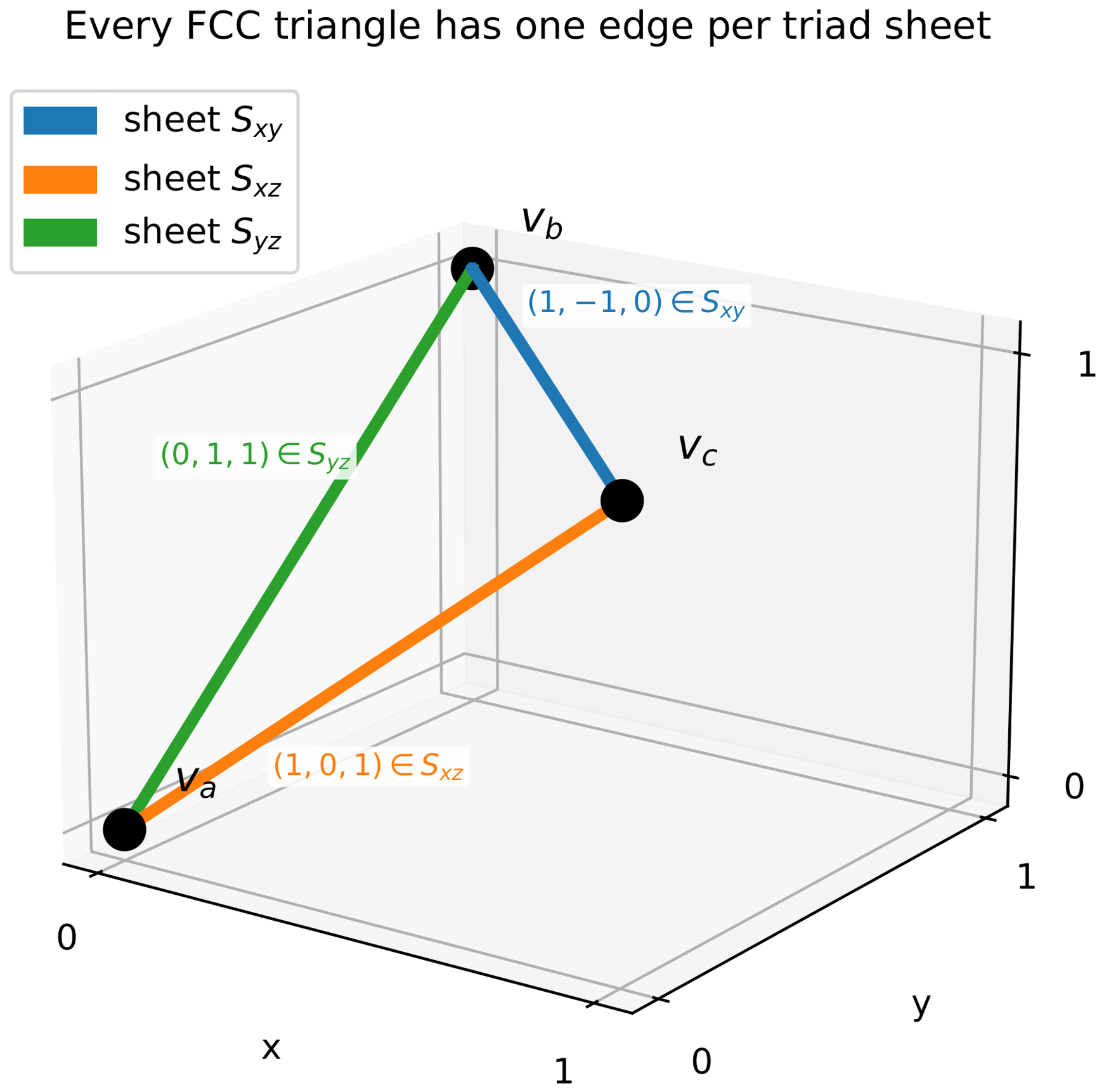
For three mutually adjacent FCC vertices (, and ), the three edge-vectors (, , and ) must each be FCC neighbor vectors. Direct case analysis on the 12 neighbor vectors shows that any three pairwise-summing-to-zero NN vectors necessarily lie in distinct sheets. Counting, each FCC vertex lies in 24 triangles, and each triangle has three vertices, so the triangle count is . Each triangle has three edges, and there are edges in total, so each edge lies in triangles. All three counts, together with the one-edge-per-sheet partition, are confirmed by direct enumeration at and . See Figure 1.
□
Figure 1.
Every FCC triangle has exactly one edge in each triad sheet. The three edge vectors of a triangle partition across , , and , as the labeled displacement vectors show. A single weight-3 Pauli measurement on a triangle simultaneously couples data qubits across all three sheets.
4.2. Triangle Operators
Definition 2
(Triangle operator). For an FCC triangle (T) with edges , , and , the Z-triangle operator is defined as
and similarly, .
A single triangle Z-operator commutes with all per-sheet Z-stabilizers but anticommutes with exactly six per-sheet X-stabilizers—two in each sheet: the triangle’s edge in a given sheet lies in exactly two octahedral voids of that sheet, and the three edges lie in three different sheets. Direct enumeration at and confirms that every one of the triangles anticommutes with exactly six. Products of triangles can be chosen to commute with all stabilizers.
4.3. Reachable Cross-Sheet Logicals
Proposition 1
(Cross-sheet reachability; dimension count verified at ). Let be the triangle-edge incidence matrix and be the cross-sheet X-stabilizer matrix. The space of valid triangle products is defined as
Then, , and admits a basis whose representatives each have support on exactly two sheets.
Origin of the . Each triangle is a 2-cell of the tetrahedral and octahedral cellulation of the 3-torus, so any triangle product lies in boundary space . The cross-sheet Z-logical space is a space of cycles, and . The three unreachable directions are exactly the global wrap cycles of the torus—one per axis—and no product of triangles can form them. This accounts for the at every L.
Scope of the two-sheet property. The basis representatives each touch exactly two sheets, and this is what the surgery protocol uses. It is not true that every element of the space does. Sums of basis vectors belonging to different sheet pairs generically touch all three: at , the sum of the first and seventh basis vectors, supported on and , respectively, has support on all three sheets. The architectural argument needs only the two-sheet basis, which is what is verified.
Verification of the dimension count: At , 21 basis logicals (out of ), all two-sheet, are distributed as 7 per sheet pair. At , 33 (out of 36), all two-sheet, are distributed as 11 per sheet pair. The is explained analytically above; the dimension count itself is checked computationally at these two sizes, which is why the statement is a proposition.
Constructive form of the two-sheet representatives. The existence of two-sheet elements does not rest on the computational check. They are built explicitly as follows.
Lemma 3
(Two-sheet primitive). For every even L and every ordered pair of distinct sheets, there is a set of L triangles whose product is supported on exactly those two sheets, with weight —namely, L edges in each.
Proof of Construction.
Every triangle has exactly one edge in each sheet (Lemma 2). Choose the L triangles as pairs, the two members of a pair sharing their edge in the third sheet. Such a pair exists because each third-sheet edge lies in two triangles whose remaining edges lie in the other two sheets. In the product over , each shared third-sheet edge appears twice and cancels, so the third-sheet edges drop out. No cancellation occurs in the other two sheets, since the L triangles contribute L distinct edges to each. The surviving support is L edges in each of the two chosen sheets, with a total weight of . □
The construction is confirmed at . In each case, the search for a minimum-weight two-sheet operator returns exactly L triangles of total weight , with third-sheet edges of multiplicity two and L edges of multiplicity one in each of the other two sheets, as the construction requires.
Proposition 2
(Per-sheet coverage; computational, verified at ). Fix a sheet (), and let denote the projection onto the Z-logical space () of those triangle-reachable logicals supported on . Then, for each partner (),
so the two-partner sheets, together, reach the full -dimensional Z-logical space of .
Verification: At , each partner pair reaches a four-dimensional subspace () of each sheet’s eight-dimensional () Z-logical space; the two subspaces intersect trivially, and their direct sum is the full eight-dimensional space. At , the same holds with . Note that this is a direct sum of subspaces: the set-theoretic union of two proper subspaces is not a subspace.
4.4. Operational Consequence
Proposition 2 is a statement about subspaces, and it is easy to read more into it than it says. The direct-sum decomposition () means that every Z-logical of sheet can be written as with and . It does not mean that ℓ, itself, lies in either summand and a generic ℓ lies in neither, nor does membership of a in mean that a can be paired with an arbitrary logical of : it means only that some partner exists. The following computation makes the actual reach explicit.
Proposition 3
(Direct reachability of basis pairs; computational, verified at ). Fix the per-sheet Z-logical bases used throughout. At each verified size (), for each basis logical (A) of a sheet (), the number of basis logicals (B) in the other two sheets such that is a triangle product is exactly L, and all L lie in one of the two other sheets, with none in the other. The total number of unordered cross-sheet basis pairs whose joint operator () is directly measurable is therefore at these sizes. The same pattern is conjectured for all even L values; no proof is given here.
Verification: At , every one of the 24 basis logicals has partner-count profile over the two other sheets, giving directly measurable pairs out of cross-sheet basis pairs. At , every one of the 36 has profile , giving out of 432. At , every one of the 48 has profile , giving out of 768, with the reachable-space dimension of , as Proposition 1 predicts. At all three sizes, exactly one-quarter of the cross-sheet basis pairs and about of all pairs are directly measurable. These three sizes are the same ones at which every threshold in this paper is simulated, so the reachability evidence and the threshold evidence cover the same range.
Operational consequence. Every basis Z-logical (and, by CSS symmetry, every basis X-logical) of every sheet has L partners with which a joint measurement can be performed by a single triangle primitive, so no basis logical is isolated. That is the whole of what the reachability results establish. Three things they do not establish are stated here so that they are not inferred. First, a basis logical reaches partners in one of the other sheets, not both. Second, it reaches L of that sheet’s logicals, not all of them. Third, a logical that is not a basis element—in particular, any sum of a component and a component is not directly reachable at all. Joint measurements outside the directly reachable pairs, of them at the verified sizes, would require either a three-sheet triangle product, which is not characterized here, or mediation through ancilla logicals, for which no protocol, depth analysis or fault-tolerance argument is given. The architecture should be read as providing a specific, structured set of cross-sheet joint measurements, not a general cross-block capability.
5. Fault-Tolerant Surgery Protocol
5.1. Ancilla Placement
Each surgery primitive uses L triangles, forming a localized cluster on the FCC lattice. For each triangle (T), A measurement ancilla is placed at the centroid of each triangle (T)’s three vertex positions, coupled to its three data qubits via short-range couplers ( at the ancilla). This fixes the ancilla’s position and connectivity; it does not fix a pulse-level or platform-specific gate scheme, and none is given in this paper. The gate schedule of Section 5.3 is stated at the level of CNOT layers and time slots. Figure 2 illustrates the canonical four-triangle primitive.
Figure 2.
Surgery primitive at . Four FCC triangles (, and ) form a closed chain around the z-direction of the torus. They share two -sheet edges, and , which appear twice in the product and cancel. The net operator has a weight of 8, with support on 4 edges in and 4 in , implementing , where A is a logical of sheet and B is a logical of sheet . Because the lattice has a circumference of 4 along z, a chain of four triangles must close through the periodic boundary: reaches and at their periodic images, i.e., and at , shown as hollow circles, with those two edges dashed. Every drawn edge is a unit nearest-neighbor bond. Red stars mark the triangle ancillas at each triangle’s centroid—’s below , where its triangle actually lies. All four ancillas are measured in the same time slot.
Fault propagation and the smallest usable L. A weight-3 measurement with single-fault propagation produces data errors of weight . Correctability of a weight-w error requires , so requires . Since L is taken as even, the smallest lattice meeting the one-fault condition is , and for , no flag qubits are needed: the per-sheet distance suffices for fault-tolerant triangle measurements.
Status of L = 4. L = 4 does not meet the one-fault condition above, and the simulated circuit contains no flag qubits. Therefore, no individual fault-tolerance claim is made for ; it enters only as a finite-size data point in the pairwise-crossing extraction of Section 7, alongside and , neither or which meets the condition. A flag-qubit protocol [10] would catch the worst-case weight-2 propagation at , but none has been implemented or simulated, and none of the reported numbers depends on it.
5.2. Connectivity Verification
Two senses of . The connectivity claim made by this paper, here and throughout, is about active connectivity per syndrome round: each data qubit participates in, at most, four two-qubit gates per round of syndrome extraction, including during surgery. This is the constraint that matters for hardware compatibility (gate scheduling, crosstalk, parallel CNOT capacity, and calibration overhead) and is what makes the architecture compatible with platforms such as Google Willow and IQM Star/Garnet, whose native processors are designed around active connectivity. The physical coupler layout of a real chip may include additional couplers (e.g., diagonal ones used only during specific phases or never used at all in this protocol); this is a separate hardware-implementation question, and no claim is made that the physical layout must literally have exactly four couplers per data qubit. Throughout this paper, “” should be read as active per-qubit connectivity during any single syndrome round.
Each data qubit therefore participates in, at most, four two-qubit gates per syndrome round, with no exceptions during surgery. During surgery, some gate slots reconfigure from per-sheet ancillas to triangle ancillas. At with the canonical 4-triangle primitive, the two -sheet edges shared between pairs of surgery triangles see two triangle-coupler gates per round (retaining two per-sheet coupler gates each); the other eight data qubits use one triangle-coupler gate with three per-sheet coupler gates retained. The active envelope is preserved throughout the surgery operation.
5.3. Gate Schedule
The triangle measurements’ CNOT gates are scheduled by coloring the conflict graph (), whose nodes are the surgery triangles and whose edges join triangles sharing a data qubit. The structure of the primitive makes this easy at every lattice size: according to Lemma 3, the L triangles form pairs, with the members of a pair sharing exactly one edge and distinct pairs sharing none, so is a perfect matching with a maximum degree of 1 and is 2-colorable. Direct construction confirms this at : two colors suffice in each case. With three CNOTs per triangle, the surgery operation therefore completes in time slots, independently of L, against six to eight time slots for a standard per-sheet syndrome extraction round. For comparison, a standard per-sheet syndrome extraction round takes six to eight time slots.
5.4. Overhead Analysis
At lattice size L:
| Quantity | Per Syndrome Round (per-Sheet) | Per Surgery Operation |
| Ancillas (3 sheets) | L measurement ancillas | |
| Two-qubit gates | to | |
| Time slots | 6–8 | ≈6 |
| Fraction of per-round cost (at ) | n/a | <0.5% |
Surgery has a subleading gate cost of two-qubit gates for the triangle measurements, compared with per syndrome round for the per-sheet stabilizer extraction.
Clock-cycle impact. Triangle measurements during the merge execute in parallel with per-sheet syndrome extraction; in a time-multiplexed schedule, triangle CNOTs occupy the same time slots as per-sheet CNOTs, without extending wall-clock time. The merge phase costs L syndrome rounds at the same clock cycle as memory, for a total surgery overhead of rounds vs. L for memory. On superconducting transmons (100–400 ns cycles [9]), rounds at is –10 µs additional wall-clock, which is well below the typical (µs); on neutral-atom platforms (ms cycles), the ms total requires sustained coherence achievable in recent demonstrations. Idle errors during merge are captured by the noise model of Section 7.
Practical reading of the overhead. The surgery primitive uses L triangle ancillas and completes in a constant number of time slots, so its cost is linear in the code distance while the block itself holds data qubits. Three consequences follow. First, the ancilla cost is asymptotically negligible: of the data budget, which is at , falling as L grows, so the primitive does not erode the code’s rate. Second, the ancillas are transient and reusable, so a device does not pay for them, except while a merge is in progress. Third and least favorably, the L triangle ancillas must be measured within the same syndrome round, so the primitive consumes L simultaneous measurement channels; on a platform where mid-circuit measurement is the scarce resource rather than qubit count, that is the binding constraint, not the qubit overhead. For comparison, surface-code lattice surgery between adjacent patches of distance d requires ancillas along the shared boundary, so the scaling is the same; what differs is that no routing region is required to bring the blocks into adjacency.
5.5. Decoder Graph
The decoder for surgery operations operates on a combined detector graph: per-sheet syndrome detectors (vertex Z, oct void X) plus triangle measurement detectors. Triangle–triangle correlations arise from shared data qubits: a Z error on a shared edge flips both triangles’ outcomes simultaneously. Standard MWPM [11] applies directly to this graph; the matcher extends the per-sheet syndrome graph with cross-sheet edges induced by triangle measurements [3,4].
5.6. Boundary Deformation: Broken Stabilizers and Their Reconstruction
A standard concern in lattice surgery is that the merge operation temporarily disrupts the per-block stabilizer structure: some stabilizers become gauge operators during the merge and must be reconstructed afterward. This disruption is characterized precisely for the FCC triangle primitive.
Lemma 4
(Broken X-stabilizers per triangle). Each individual triangle (T) with edges , and —one per sheet—anticommutes with exactly six per-sheet X-stabilizers: the two octahedral voids in each sheet that contain one of the triangle’s edges. The breakdown is two X-stabilizers in , two in , and two in .
Proof.
A triangle Z-operator () acts on three edges. Each edge () is contained in exactly two octahedral voids of , since each FCC edge connects two oct-void neighbors. The X-stabilizer of an oct void contains e as one of its four support edges. Therefore, overlaps each such X-stabilizer in exactly one edge (odd) and anticommutes with it. The six X-stabilizers (two per sheet) are distinct, since they correspond to distinct oct voids. □
Gauge structure during surgery. During the multi-round merge, the L triangles of the surgery primitive collectively anticommute with distinct per-sheet X-stabilizers (each broken by exactly two triangles, accounting for the total triangle-stab anticommutations of Lemma 4). These X-stabilizer measurements become gauge bits during the merge: their outcomes are correlated with the triangle outcomes but do not constrain the merged code’s logical subspace. Verified numerically:
| Triangles in Primitive | Distinct X-Stabs Broken | Per-Triangle Broken | Net Broken | |
| 4 | 4 | 12 | 6 | 0 |
| 6 | 6 | 18 | 6 | 0 |
The three columns count different things. Per-triangle broken is the number of X-stabilizers a single triangle anticommutes with, which is 6 according to Lemma 4—two in each sheet. Distinct X-stabs broken is the size of the union over the L triangles of the primitive, that is, how many different X-stabilizers are touched at least once. Net broken counts those touched an odd number of times, i.e., those actually broken by the product.
The arithmetic at illustrates the following relation: 4 triangles anticommutations incidences, spread over 12 distinct X-stabilizers, so each is touched exactly twice. Twice is even, so nothing is net-broken. This is not a coincidence of : the product of commutes with every X-stabilizer by construction (Proposition 1), and commuting with a stabilizer is exactly the statement that the number of anticommuting factors is even. The net-broken column is therefore zero at every L, which is what makes the merge a valid stabilizer measurement rather than a state-destroying one.
Post-merge reconstruction. After the d-round merge phase, the initially broken X-stabilizer outcomes are reconstructed from the L triangle measurement outcomes plus surviving stabilizer constraints: each broken X-stabilizer’s eigenvalue is the modulo-2 sum of (i) its pre-merge eigenvalue, (ii) the triangle measurements whose Z-operators overlap it in odd parity, and (iii) propagated Pauli corrections from the surgery protocol. This is the FCC-triangle analog of the standard rough/smooth boundary deformation in surface-code lattice surgery [3]: per-sheet boundary stabilizers are temporarily opened as gauges and closed upon surgery completion. No per-sheet stabilizer is permanently modified; the affected weight-4 stabilizers are still physically measured throughout the merge, but their round-to-round detector constraints are gauge-dependent during the merge window and are therefore omitted from the DEM during that window (see Section 7.1); they are restored post merge using the triangle-outcome records described above.
Single-fault error propagation across sheets. A single fault on a triangle ancilla mid-circuit can propagate to, at most, two data qubits in different sheets: for the canonical CNOT schedule, i.e., , a Z error on the ancilla after the CNOT and before the CNOT propagates to one data qubit each in and . This weight-2 cross-sheet error triggers detectors in two distinct per-sheet syndrome graphs; the decoder graph must include edges spanning these per-sheet graphs (Section 7).
6. Distance Preservation
Theorem 3
(Merged code distance). For any even and any cross-sheet measurement operator () implemented by a weight- triangle product, with supported in sheet and in sheet (), the merged code formed by adding as a Z-stabilizer has stabilizer rank increased by exactly 1 (consuming one logical qubit), and the minimum-weight logical operator of the merged code has a weight of L. Distance is preserved.
Proof.
Stabilizer rank. commutes with all original X-stabilizers according to Proposition 1 (it is the product of triangle Z-operators chosen to be in the joint kernel of ). is not in the row span of , since it is a non-trivial element of the Z-logical group. Therefore, appending to increases the rank by 1, and the merged code has logical qubits.
Minimum logical weight. The merged Z-logical group is the original Z-logical group quotiented by the subgroup. Each non-trivial equivalence class has the form of for a representative g in the original Z-logical group, with g not equivalent to modulo the original stabilizers.
Decompose any g as , where denotes the restriction of g to sheet . Similarly, decomposes as with of weight L in and of weight L in . Then,
where k is the third sheet ().
According to the Layer Decomposition Theorem (Theorem 2), each non-trivial logical () on sheet has a weight (per-layer 2D toric code distance).
Since g is non-trivial in the merged code, at least one sheet restriction () must be a non-trivial logical of that sheet: if every were trivial, then g would be a product of per-sheet stabilizers and, hence, trivial, and the class would be the trivial class of the merged code. The cases below are therefore exhaustive:
- (a)
- , i.e., is a non-trivial logical of . Then, . Both and contain as a summand, so the class minimum is .
- (b)
- is trivial in (i.e., or a stabilizer), but is a non-trivial logical of . Then, , so . For , the contribution of is either (if and are in distinct logical classes or if is a stabilizer leaving the contribution of weight L) or zero (if ). In the zero case, has contributions only from (in , weight ) and (in , possibly weight 0). Therefore .
- (c)
- By symmetry with (b), interchanging i and j.
- (d)
- Multiple sheets contribute non-trivial logicals. Then, both and inherit contributions from at least two non-trivial per-sheet logicals, each , so the class minimum is .
Achievability of . The class containing has representatives . Since modulo per-sheet stabilizers, this class equals , with representatives each of weight L. Therefore, the minimum is achieved. □
Computational verification. The proof above is independent of L. To rule out edge cases, Theorem 3 was additionally checked by exhaustive enumeration at small L values. At , all per-sheet logical generators give a class minimum of exactly 4, and the same minimum holds for all pair products. At , all 36 generators and pair products give a class minimum of exactly 6. No combination produced a class minimum below L.
X-Distance Preservation
Theorem 3 addresses the Z-logical group of the merged code, which is the side directly modified by the cross-sheet Z-measurement (). The X-side requires a separate argument: the merged X-logical group is the subgroup of the original X-logicals that commute with , modulo the original X-stabilizers (which are unchanged by the surgery).
Theorem 4
(X-distance preservation). Under the same conditions as Theorem 3, the merged code’s X-distance equals L (the per-sheet code distance). The merged code’s X-logical group consists of all original X-logicals that have even overlap with the support of , modulo the (unchanged) X-stabilizer group.
Proof.
Setup. The original code has X-stabilizer matrix and Z-logical group , as well as X-logical group . After surgery, the merged code has stabilizer matrices (unchanged) and . The merged X-logical group is the normalizer of the merged stabilizer group restricted to X-type operators, modulo the merged X-stabilizers:
The commutativity condition of for g, an X-operator and a Z-operator reduces to: g has even-parity overlap with the support of .
Counting. The original X-logical group has generators ( per sheet for the toric code; L per sheet for the planar variant). , where A is a Z-logical of sheet and B is a Z-logical of sheet . X-logical (the conjugate of A in ) anticommutes with (per-sheet anticommutation) and commutes with (disjoint sheet supports), so anticommutes with . Symmetrically, anticommutes with . All other generators of commute with : per-sheet X-logicals in sheets , have disjoint support from and commute trivially; per-sheet X-logicals in or other than or are independent of (resp. ), and the per-sheet anticommutation structure ensures they commute with the relevant component of .
The merged X-logical group has commuting generators from the original , but the product of (sum of two anticommuting generators) commutes with (and anticommutes with each component, so even total overlap). This product is a non-trivial X-logical of the merged code, representing the consumed-Z logical’s X-conjugate. Thus, the merged X-logical group has generators, consistent with (one Z-logical consumed by adding ).
Minimum weight. The merged X-logical generators are of two types:
- (a)
- Original per-sheet X-logicals that commute with : weight of L each (per-sheet 2D toric distance, Theorem 2).
- (b)
- The new generator (): weight of (disjoint supports across sheets and ).
The minimum weight over all generators is L. For arbitrary linear combinations, the following argument applies, spelled out here because counting generators alone does not establish it.
Let be any non-trivial logical X-operator of the merged code. According to Theorem 2, each sheet is a direct sum of L independent rotated toric layers, and the merge adds triangle operators without coupling distinct layers, so the merged X-stabilizer group is likewise layer-decomposable. is restricted to a single-layer ℓ, and the restriction is called . Each either lies in that layer’s stabilizer group or is a non-trivial logical operator of it.
Suppose every lays in its layer’s stabilizer group. Then, , being their union over disjoint supports, would lie in the merged stabilizer group and, hence, be trivial, contrary to assumption. Therefore, at least one layer () has non-trivial logical operators. That layer is a rotated toric code of distance L, so . Since the layers have disjoint support, . Combined with the generator with a weight of exactly L, the merged X-distance is L. □
Computational verification. At , all X-logical generators have a weight of L; exactly two anticommute with (confirming the count of single-generator commuters), and the minimum weight among merged X-logical generators is exactly L. Combined with Theorem 3, the merged code distance is L for both Z- and X-side errors.
7. Threshold Simulation
The surgery operation is characterized using a custom Stim circuit [12] with explicit triangle measurements, decoded with MWPM via PyMatching [11], and a finite-size-scaling (FSS) crossing threshold estimate is extracted from pairwise crossings at . The static memory FSS-crossing estimate is reported as a complementary baseline.
7.1. Custom Stim-Circuit Construction
A Stim circuit is constructed implementing the full surgery operation. A merge joins two logical qubits, so the merge circuit acts on two triad sheets ( for the primitive), with the third sheet contributing only the remaining edge of each triangle as an auxiliary data qubit; the three-sheet CNOT of Section 10 is where all three sheets carry logical qubits at once. The circuit has per-sheet vertex Z- and oct-void X-stabilizer measurements, L triangle ancilla measurements during the merge phase, and auxiliary data qubits used by the triangle measurements. Three phases of d syndrome rounds (pre-merge, merge, and post merge) and the X-stabilizers broken during merge (Lemma 4) have detectors skipped per the gauge structure of Section 5.6. Key statistics:
| Total Qubits | Triangles | Broken X-Stabs | DEM Error Mechanisms | |
| 4 | 324 | 4 | 12 (8 in , 4 in ) | 23,946 |
| 6 | 750 | 6 | 18 (12 in , 6 in ) | 70,434 |
| 8 | 2568 | 8 | 24 (16 in , 8 in ) | 539,215 |
The DEM decomposes via Stim’s decompose_errors=True (hyperedges into graph-like edges where possible) at all three sizes; the resulting graphs are compatible with PyMatching’s MWPM decoder.
7.2. Circuit-Level Noise Model
Every number in this section comes from a Stim circuit built by sheet_code_custom_surgery.py, with a single uniform parameter (p) applied to all channels. Explicitly:
| Location | Stim Channel | Rate |
| After reset (data, per-sheet ancillas, and triangle ancillas) | DEPOLARIZE1 | p |
| Idle ancillas between phases | DEPOLARIZE1 | p |
| Every two-qubit gate (syndrome extraction and triangle CNOTs) | DEPOLARIZE2 | p |
| Before each ancilla measurement | X_ERROR | p |
| Before the final destructive data measurement | X_ERROR | p |
So p is simultaneously the one-qubit depolarizing rate, the two-qubit depolarizing rate, the measurement flip probability and the reset error probability. There is no separate idle rate: idling ancillas take the same DEPOLARIZE1 channel. Leakage, crosstalk and correlated errors are not modeled. Detector error models are generated by Stim and decoded with MWPM (PyMatching) on the decomposed graph. Reported logical error rates are per surgery operation, not per round.
7.3. Surgery Operation Threshold
Terminology. The numerical threshold estimates throughout this section and the rest of the paper are finite-size crossing estimates extracted from pairwise crossings of logical error rates at with MWPM decoding. The abbreviation of FSS-crossing estimate or, simply, “threshold estimate” is used for compactness. These are not asymptotic () thresholds. They are empirical crossings at three accessible code distances. The quoted uncertainty is the spread of the three pairwise crossings, together with a formal FSS data-collapse fit where available (Section 9.2 for the planar variant; the toric FSS fit gives , , which is statistically consistent with the pairwise-crossing estimate). Extending to or would tighten the band but is computationally expensive (Section 10.8).
Z-basis logical memory experiments are performed with the joint observable expressed as (the cross-sheet logical that the surgery primitive measures), running syndrome rounds (pre-merge d, merge d, and post-merge d) followed by destructive Z-measurement. Three code distances were measured: .
| (%) | |||
| 0.10 | (0/500) | (0/1000) | |
| 0.20 | (0/1000) | ||
| 0.30 | (0/1000) | ||
| 0.40 | n/a | n/a | |
| 0.50 | |||
| 0.60 | n/a | n/a | |
| 0.70 | |||
| 0.80 | |||
| 0.90 | |||
| 1.00 | |||
| 1.10 | |||
| 1.20 | |||
| 1.50 |
Pairwise crossings and threshold estimate. The pairwise crossings of vs. , vs. , and vs. give three independent estimates:
| Crossing | |
| vs. | |
| vs. | |
| vs. |
The three crossings span to . The finite-size threshold estimate is , where the band reflects the spread of pairwise crossings. Below threshold, the d-scaling is monotonic with L: at , the logical error rate is at , at , and at , decreasing as expected for a fault-tolerant operation in the below-threshold regime.
A crossing that excludes . Section 5 notes that does not satisfy the one-fault condition, so the crossing that does not involve it is isolated here. Of the three pairwise crossings, i.e., ( vs. 6), (4 vs. 8) and (6 vs. 8), only the last uses solely sizes that meet the condition, and it sits at . The percentage-level conclusion therefore does not rest on the data: is retained as the three-size estimate, and is reported alongside it as the FT-size-only check.
Formal FSS fit. As a second, parameterized threshold estimate, the standard finite-size scaling ansatz is fitted as with to the near-threshold data (, 21 data points across ) by least squares with weighted residuals (shot-noise statistical errors). The fit yields
with . Consistent with the pairwise estimate within combined uncertainty (fit centered ∼0.07% higher). The exponent of is in the percolation universality range expected for surface-code-like threshold transitions ( to [13]). The indicates systematic deviations from the simple quadratic ansatz typical of surface-code FSS at moderate L values. The pairwise-crossing estimate is the more conservative (model-free) report; both are stated for completeness.
Shot counts and methodology. Each row uses at least 1000 shots; near-threshold rows (–) use up to 8000 shots for tighter confidence intervals. The standard error on each rate is plotted in Figure 3 as a Wilson 95% interval, which remains positive at the low-count points.
Figure 3.
Surgery threshold from the custom Stim circuit with explicit triangle measurements at . Each point uses the full surgery protocol of rounds of pre-merge, merge with triangle measurements, and post-merge, with MWPM decoded on the decomposed DEM. Data are from threshold_summary.csv. Error bars are Wilson intervals, which are asymmetric and remain positive at the low-count points. Points at which no logical failure was observed cannot be placed on a log axis and are shown as open triangles at their upper bound. The three pairwise crossings of vs. , vs. and vs. occur at , and (gray band), giving .
7.4. Comparison with Proxy Estimate
Before presenting the simulated value, a crude expectation is useful to compare against. A natural proxy is to treat the merge as though it were an ordinary surface-code memory experiment of the same duration: take a single rotated surface code at distance L; run it for rounds, which is the same total syndrome budget the merge consumes; and ask at what physical error rate its logical error rate stops improving with L. Standard rotated surface-code memory has a circuit-level MWPM threshold near for a single round; running rounds instead of d multiplies the number of opportunities for a logical failure by three, which shifts the crossing down by roughly a factor of two, giving . This is an order-of-magnitude expectation, not a simulation, and it is quoted only to show that the measured value exceeds rather than merely matches the naive guess. The custom Stim circuit gives a pairwise-crossing estimate of , and the collapse fit is ; both are roughly twice the proxy. The proxy is conservative for three reasons. It assumes the joint observable fails as often as rounds of single-cycle memory, which ignores the robustness of the -qubit cross-sheet support. It treats a single 2D code as a stand-in for the sheet code, which ignores the layer decomposition (Theorem 2), where per-layer X-errors do not propagate. And it discards the role of the triangle measurements as auxiliary syndrome bits during the merge.
7.5. Static Memory Threshold (Single-Sheet Baseline)
For comparison with the surgery threshold, a single-sheet static memory experiment was also run using a custom circuit with no triangle measurements. What this is and is not should be clear at the outset. Data exist at two lattice sizes only ( and ), and a crossing extracted from two curves is an interpolation between them rather than a finite-size scaling estimate: with two sizes, there is no scatter from which to estimate an uncertainty, and no way to detect curvature. The number is therefore reported as a consistency check against the rotated toric code that the sheet code reduces to and not as a threshold estimate. It is not used to support any claim in this paper. Z-basis memory experiment with d syndrome rounds on the sheet at and :
| (%) | , | , |
| 0.10 | ||
| 0.30 | ||
| 0.50 | ||
| 0.80 | ||
| 1.20 |
The single-sheet static memory two-size interpolation from this custom circuit at sits near , statistically consistent with the surgery FSS-crossing estimate of and with the surface-code-literature threshold ( at MWPM under circuit-level depolarizing noise).
7.6. Decoder: What Is Verified and What Remains Open
The custom Stim circuit of Section 7.1 produces a decomposable detector error model (23,946 error mechanisms at surgery). Verified: (a) The DEM can be decomposed into an MWPM-compatible graphlike model via decompose_errors=True (a two-edge decomposition of the cross-sheet hyperedges; this addresses the principal Section 5.6 concern that surgery introduces hyperedges, but the decomposition, itself, can be lossy. Optimal hypergraph or BP+OSD decoding remains open); (b) MWPM via PyMatching gives the threshold estimate of at ; (c) the broken-X-stabilizer detector handling produces a deterministic detector pattern combined with triangle outcomes. Open: (i) Whether BP+OSD [14] extracts a higher FSS-crossing estimate from the same DEM (the hyperedge decomposition is lossy); (ii) larger-L behavior (, computationally expensive); (iii) a full three-sheet rather than two-sheet circuit (the sheet supplies only auxiliary triangle data qubits in this circuit, and the estimate is expected to be unchanged); (iv) decoders specific to the FCC sheet code’s octahedral symmetry. The custom Stim circuit confirms fault-tolerant operation under MWPM at FSS-crossing estimates in the same hardware-compatible regime as the surface code.
8. Comparison with State of the Art
8.1. Practical Position
Limits of the sheet code. The sheet code is not a constant-rate qLDPC code: its rate of vanishes as —the same asymptotic scaling as the surface code. Bivariate bicycle codes and recent “good” qLDPC codes achieve constant or growing rates at higher connectivity ( or higher with long-range couplers). The sheet code does not solve the asymptotic rate problem.
Contribution of the sheet code. What the sheet code does provide is native cross-block fault-tolerant joint Pauli measurements at active connectivity, with FSS-crossing threshold estimates comparable to single-block surface-code memory. Surface-code lattice surgery provides these primitives only within a single substrate; bivariate bicycle codes target inter-block operations at with active research on the inter-block protocols. The sheet code offers a third option: inter-sheet joint Pauli measurements between logically distinct but co-located CSS code blocks, native at via local triangle measurements. The trade is explicit: toric-code-level rate and toric-code-level memory performance, at surface-code connectivity, in exchange for a cross-block joint Pauli primitive that neither the surface code nor a plain toric stack provides between separated blocks. Composing these primitives into full FT logical Clifford gates (e.g., a fault-tolerantly thresholded CNOT) requires the additional protocol refinements identified in Section 10 and is not established by this work.
8.2. Quantitative Comparison Table
Figure 4.
Data qubits per logical qubit at matched distance, the fair axis for comparing code densities, with the cross-block primitive annotated. (The routing comparison of Section 8.4 uses physical qubits instead because a routing reservation is an ancilla cost and is invisible on this axis). The sheet code and the rotated 2D toric code coincide exactly at , as Theorem 2 requires: the sheet code is a stack of rotated toric codes. The factor of two separating both from the rotated surface code is the periodic-boundary factor, not an FCC effect. Bivariate bicycle is denser still, at with long-range couplers. The distinguishing property is the rightmost column: “structured cross-sheet pairs” means joint Pauli measurement between logical qubits in distinct code blocks with no routing for the basis pairs of Proposition 3 at and not for arbitrary logical pairs. Surface-code patches must instead be adjacent, or the architecture must reserve routing space.
Table 2.
Comparison of CSS codes at code distance d (or L). The rate is . Note the rate parity: the sheet code and the rotated 2D toric code both sit at , as Theorem 2 requires, and the planar sheet code matches the rotated surface code at . The distinguishing column is the cross-block primitive, not the rate. “Wraps” indicates that periodic boundary couplers ae required. “Cross-block primitive” denotes the available primitive for operations between independent code blocks: lattice surgery within a patch for surface code, FT joint Pauli measurements via triangle surgery for the sheet code, and active development for bivariate bicycle. The Gross BB code uses fixed values of , , and .
8.3. Trade-Offs and Practical Niche
Where the sheet code wins. (i) Cross-block joint Pauli measurements at with short-range couplers only and without a routing reservation, worth a factor of in physical qubits per logical qubit against a bussed toric array at matched distance (Section 8.4): Three code blocks share one FCC geometry, and a weight-3 triangle reaches one data qubit in each, so a structured set of cross-block pairs, basis pairs at the verified sizes according to Proposition 3, is joinable with no routing. Surface-code lattice surgery gives the same primitive between adjacent patches, but arbitrary pairs need reserved routing space. Here, no routing space is needed for the directly reachable cross-sheet pairs. (ii) Connectivity versus bivariate bicycle: BB codes obtain inter-block operations at with some long-range couplers [6]; the sheet architecture needs in plane plus short vertical bonds at triangle ancillas only. (iii) Distance scaling versus the parent code. Unlike the FCC code’s fixed , the sheet code has ; and unlike the 3D toric code’s at , it carries per sheet.
Where the sheet code claims nothing. It offers no memory or density advantage over stacked rotated toric codes: according to Theorem 2, it is such a stack, and the qubits-per-logical figures are equal at every distance (Section 2.5). The factor of two over the rotated surface code is the periodic-boundary factor and is not FCC-specific; the planar variant, which is what planar hardware can actually run, has no density advantage at all. Its memory threshold is the toric code’s, and the measured static crossing near is consistent with that rather than an improvement on it.
8.4. Value of the Cross-Sheet Primitive
The memory offers no advantage over a stack of rotated toric codes, as Section 2.5 states. The advantage is elsewhere, and since it is the paper’s only claim to novelty, it is stated here as a quantity rather than a description.
Note on the axis. Figure 4 counts data qubits per logical qubit, which is the right axis for comparing code densities. The comparison below counts physical qubits—data plus ancillas—because a routing reservation is an ancilla cost and would be invisible on a data-only axis. For the sheet code, the two differ by a factor of two, since each sheet carries one vertex and one void ancilla per two data qubits: data qubits per logical at becomes physical qubits per logical.
The comparison that matters. A rotated toric array performs lattice surgery only between adjacent patches. An architecture that must join arbitrary pairs therefore reserves routing space, and standard layouts budget approximately tiles per logical qubit for a compact routing bus and 2 for a fast one [4]. That reservation carries no logical qubits of its own and is paid whether or not a merge is in progress.
Routing-free reach of the sheet architecture. For the pairs that a single triangle primitive can join and only for those, the routing reservation is unnecessary. Proposition 3 fixes what that set is at : cross-sheet basis pairs, with each basis logical reaching L partners in one other sheet. The formula of is used below for general L values as a conjecture supported by those three sizes, and every number quoted at is a verified one. For those pairs and at a matched distance of , the sheet architecture uses physical qubits per logical qubit, against for a bussed toric array, i.e.,
independent of lattice size. Table 3 gives the numbers.
Table 3.
Physical qubits per logical qubit at matched distance—data plus ancillas. The factor of applies only to joint measurements within the directly reachable set of Proposition 3; for other pairs, the sheet architecture also needs routing, and no advantage is claimed.
Scope of the factor. The reachable set is smaller than an earlier version of this section assumed. With logical qubits, there are pairs in total, of which join logicals in different sheets. Only of those—one-quarter of the cross-sheet pairs and about of all pairs—are directly measurable at the verified sizes: at , that is 192 pairs out of 1128, a computed value rather than an extrapolated one. The remaining cross-sheet pairs are not reachable by any two-sheet triangle product, same-sheet pairs are not reachable by any triangle product, and no routing protocol is given for either. For those pairs, the sheet architecture would need routing exactly as a toric array does, and Equation (6) does not apply.
The honest comparison is therefore not architecture-wide. A rotated toric array with no routing space reaches only physically adjacent patches; the sheet architecture with no routing space reaches a different and structured set, with L partners per logical in one other sheet and those partners lying in a different code block rather than an adjacent patch of the same block. Which set is more useful depends on the workload. For a workload whose joint measurements lie within the directly reachable set, such as parity checks between corresponding logicals of two blocks, the routing reservation is avoided and the factor of is real. For a general workload, it is not.
Operational consequences: a logical interconnect. The practical reading of the reachable set is as an interconnect between independently encoded blocks. A logical Bell measurement on a pair consists of measuring and ; the -merge and -merge characterized in Section 7 and Section 9.3 are exactly those two measurements, each with its own finite-size threshold. For any pair in the reachable set, the architecture therefore provides the two ingredients of fault-tolerant entanglement generation and logical parity measurement between co-located blocks, with no routing region. Two qualifications belong here. First, the end-to-end Bell measurement is not simulated in this paper; what is characterized is each merge separately. Second, unlike the composed CNOT of Section 10, a Bell measurement records its two outcomes rather than feeding a Pauli-frame correction into a subsequent gate, so the failure mode identified there, unprotected single-record gauge measurements driving a correction, does not arise in the same way. That is an argument about the circuit structure, not a simulation result. The interconnect does not give general Clifford circuits because the composed CNOT is not yet fault-tolerantly characterized.
Costs. The comparison assumes the bussed array is built in two dimensions and the sheet architecture is built in three. Three-layer stacking with vertical couplers at the triangle ancillas is a real engineering cost that qubit counting does not capture, and a reader weighing the two should weigh it alongside Equation (6).
Where the sheet code loses. (i) Asymptotic rate vs. qLDPC: The rate vanishes as , with the same as surface code; bivariate bicycle achieves a rate at and recent “good” qLDPC codes at . At , the Gross BB code’s rate () is approximately higher than the sheet code’s at the same distance. (ii) The toric variant needs wrap couplers; the planar variant has half the rate (L logicals per sheet). (iii) Partial logical reachability via triangles: products span of the cross-sheet logicals (three global-wrap correlations are unreachable); same-sheet pairs are not reachable by any triangle product, and no routing protocol, depth analysis or FT argument for a routed operation is given here. (iv) Threshold simulation uses MWPM on a decomposed DEM; BP+OSD may extract further improvement.
Practical niche. The practical niche is hardware with active connectivity (Google Willow [9] and future surface-code-compatible deployments); code distances of , where bivariate bicycle’s overhead is not yet justified; and workloads requiring frequent inter-sheet joint Pauli measurements, where surface code patches would force routing or transversal protocols across separate substrates. For longer-term, larger-scale fault tolerance () on hardware, bivariate bicycle codes remain preferable.
8.5. Noise Model Scope: Markovian Depolarizing Noise
Every number in this paper comes from a uniform circuit-level depolarizing model: a single parameter (p) applied as DEPOLARIZE2 on two-qubit gates, DEPOLARIZE1 on single-qubit locations, and X_ERROR on reset and measurement. This model is Markovian and spatially uncorrelated by construction, and it is the standard basis for comparison across the surface-code literature, which is why it is used here. It is not a hardware model.
Real devices depart from it in ways that matter for thresholds. Non-Markovian dynamics, in which the environment retains memory between syndrome rounds, can correlate errors across rounds and invalidate the independent-fault counting that underlies both matching decoders and the distance argument [16,17,18,19]. Spatially correlated faults, such as crosstalk between neighboring couplers or leakage that migrates between qubits, break the assumption that the three sheets fail independently, which underlies the per-sheet rates quoted here. Both effects generally reduce the achievable threshold relative to the depolarizing value, and neither is captured here.
This bears directly on the stacked-hardware discussion of Section 3. The isolation of the three sheets in this work is logical isolation by construction: the sheets are edge-disjoint, and no error channel in the simulated model couples them. That is a property of the model, not a demonstrated property of any device. Establishing that a stacked three-layer implementation actually achieves comparable inter-layer isolation would require the measurement of crosstalk and correlated-error rates between layers on real hardware, which is outside the scope of this work. Therefore, no claim is made that the quoted thresholds transfer to a stacked device.
9. Discussion
9.1. Universal Gate Set
Joint Pauli measurements are sufficient in principle to synthesize arbitrary Clifford operations through standard lattice-surgery protocols with ancilla logical qubits [3,4]. In this work, the three-sheet Horsman CNOT logical truth table is verified (Section 10) at , but the composed protocol is not yet fault-tolerantly thresholded (its -scaling fails because the Pauli-frame correction enters the observable through single-record gauge measurements). Establishing FT-thresholded Clifford composition and, by extension, a fault-tolerantly characterized universal Clifford set therefore requires the gauge-measurement refinement or the transversal route discussed in Section 10.5, neither of which is provided here. Non-Clifford gates (such as T) further require magic-state injection or distillation; the FCC lattice’s high symmetry group (octahedral, order 48) may support efficient magic-state protocols, but no such protocol is constructed here, and a detailed analysis is left to future work.
9.2. Planar-Boundary Surgery
For real hardware deployments without periodic boundary conditions, each layer becomes a rotated surface code with rough/smooth boundaries: rough on and smooth on for , rough on and smooth on for , and rough on and smooth on for . The rough-on-z choice for aligns the rough boundary with the direction in which the triangle primitive’s chain extends (the primitive cancels -sheet edges and extends through L layers along z), enabling a non-trivial cross-sheet logical to terminate on rough boundaries.
Verified parameters. The planar code satisfies ; the minimum-weight cross-sheet surgery primitive at :
| Data Qubits () | Logicals () | Distance | Triangles in Primitive (Op Weight) | |
| 4 | 108 | 12 | 3 | 9 (21) |
| 6 | 450 | 18 | 5 | 25 (55) |
| 8 | 1176 | 24 | 7 | 49 (105) |
The planar per-sheet logical count is L (one per layer), so the three-sheet code encodes vs. in the toric construction. The planar distance scales as (standard rotated surface code finite-size effect). The minimum-weight naive surgery primitive uses triangles, producing an Op of weight (a thick block rather than the toric ribbon), forced by the additional boundary-stabilizer commutation constraints.
Measured planar threshold. Following the same custom Stim methodology as the toric case, planar surgery logical-memory experiments are run with rounds of syndrome extraction. The naive -triangle primitive (commuting with all boundary stabs) yields no d-scaling crossing across , with shot counts up to 30,000 (logical error rate strictly increasing in L at every measured p, implying a threshold below , dominated by the -weight Op being too heavy to protect).
Boundary-aware planar primitive. The primitive involves allowing the primitive’s Z-operator to anticommute with one weight-2 boundary X-stab, treating it as an additional broken stabilizer during the merge phase, in direct analogy to the toric protocol’s bulk-broken X-stabs (Lemma 4). This dramatically reduces the primitive’s Op weight:
| Triangles | Op Weight | Boundary Stabs Broken | Total Qubits | Total Broken X | DEM Mech. | |
| 4 | 3 | 7 | 1 | 175 | 6 | 11,688 |
| 6 | 5 | 11 | 1 | 757 | 10 | 41,183 |
| 8 | 7 | 15 | 1 | 1987 | 14 | 137,904 |
The boundary-aware primitive is a ribbon structure with an Op weight of and triangle count of , closely analogous to the toric primitive (Op weight of , triangle count of L). It breaks exactly one additional weight-2 boundary X-stabilizer per surgery operation, handled by the same detector-suppression mechanism used for bulk-broken X-stabs.
Logical error rates per surgery operation under MWPM decoding with the boundary-aware primitive:
| (%) | |||
| 0.10 | |||
| 0.20 | |||
| 0.30 | |||
| 0.50 | |||
| 0.70 | |||
| 0.80 | |||
| 0.90 | |||
| 1.00 | |||
| 1.10 |
Pairwise crossings and threshold estimate.
| Crossing | |
| vs. | |
| vs. | |
| vs. |
The three crossings span to , giving for the boundary-aware planar variant (Figure 5). This is lower than toric (), reflecting the cost of boundary-stabilizer breaking, but in the same percentage-level regime. For reference, Google’s distance-7 Willow demonstration reports a two-qubit CZ error rate of ≈0.36% [9], which is numerically below both FSS-crossing estimates. This is not a like-for-like comparison: the parameter p here is a single uniform parameter in the model of Section 7.2, whereas a hardware comparison requires a platform-specific noise model including measurement, reset, idle, leakage and correlated errors.
Figure 5.
Planar-boundary surgery threshold with the boundary-aware ribbon primitive at . The boundary-aware variant allows exactly one weight-2 boundary X-stabilizer to be broken during the merge, in direct analogy to how the toric protocol breaks bulk X-stabilizers (Lemma 4). Data are from planar_ba_threshold_results.json, with repeated runs at the same merged; error bars are Wilson intervals. The three pairwise crossings of vs. , vs. and vs. occur at , and (gray band), giving .
Formal FSS fit (planar). Applying the same FSS ansatz to the boundary-aware planar data (, 21 data points across ) gives
with .
Fit diagnostics. Because three lattice sizes is the minimum from which a five-parameter collapse can be attempted, the full set of diagnostics is reported rather than the central value alone. The ansatz is with , five free parameters (), fitted by weighted least squares with binomial weights to points inside the stated window with at least five observed failures. Table 4 gives the sensitivity of the result to the included data.
Table 4.
Finite-size-scaling fit diagnostics. Rows differ only in which data are included. The quoted uncertainties are the covariance-matrix errors; since exceeds unity in both datasets, the values reported in the text are these errors scaled by .
Does including bias the estimate? Section 5 notes that does not satisfy the one-fault condition, so it is reasonable to ask whether its inclusion distorts the threshold. Two independent checks say the effect is present but smaller than the finite-size scatter. First, on the pairwise crossings: the three crossings are , and , with a mean of and spread of , while the only pair that excludes gives . The shift is percentage points, or times the spread. Second, on the collapse fit, dropping moves from to , a shift of combined standard errors, while is unchanged within its uncertainty. is therefore retained in the headline estimate, with the versus crossing alongside it. Note that every estimate quoted in this paper would move down by roughly one standard error if were excluded throughout. The fit-based threshold coincides with the lowest pairwise crossing ( vs. at ), reflecting the additional weight that low-L data carries in a quadratic fit. The exponent of matches the toric value within uncertainty, as expected for a CSS-symmetric construction.
Comparison summary.
| Variant | Triangles | Op Weight | Distinct Broken X | DEM Mech.() | |
| Toric | L | 539,215 | |||
| Planar (naive) | 325,423 | ||||
| Planar (boundary-aware) | 137,904 |
The boundary-aware planar variant achieves toric-comparable thresholds with strictly planar (no-wraparound) hardware, deployable on Google Willow-class platforms without toric topology. The threshold reduction relative to toric variant is the cost of handling boundary stabilizers; further optimization (e.g., distributing broken stabs across both blocks of a multi-block surgery) is future work.
9.3. XX-Merge: The CSS-Symmetric Surgery Primitive
The triangle primitive that implements the ZZ-merge (Section 7) has a CSS dual: replace the triangle ancilla protocol with the X-basis version. Ancilla is reset to , the CNOT direction is reversed (ancilla as control, data as target), and ancilla is measured in X. To obtain an XX-merge primitive measuring the joint X-product of triangle data qubits, the constraint becomes the following: triangle combinations whose X-product commutes with all Z-stabilizers and is not in the row span of .
Primitive identification (toric). Searching the kernel of at minimum weight, after skipping trivial X-stabilizer combinations, yields the following:
| ZZ-Primitive (tri, wt) | XX-Primitive (tri, wt) | Broken Stabs | Notes | |
| 4 | 4, 8 | 4, 8 | 12 Z-stabs | Exact CSS mirror |
| 6 | 6, 12 | 6, 12 | 18 Z-stabs | Exact CSS mirror |
| 8 | 8, 16 | 8, 16 | 24 Z-stabs | Exact CSS mirror (pinned pair) |
At the XX-primitive structurally mirrors the ZZ-primitive exactly: same triangle count, same operator weight, and the same distinct broken Z-stabilizers per surgery (the CSS dual of the ZZ-primitive’s broken X-stabs, Lemma 4). At , minimum-weight search returns a two-sheet artifact (weight 16, sheets only); the first three-sheet primitive appears at higher weight (10 triangles, weight 20), breaking 28 Z-stabs.
Threshold measurement. Threshold measurement involves a custom Stim circuit with syndrome rounds, initialization, and final X-basis readout. Z-stab detectors are paired from round 1+, except the ones broken during the merge phase (24 at ); X-stab detectors are deterministic in round 0 and paired throughout. Logical error rates are recorded per surgery operation, with the merged sheet pair pinned to at every size (see below):
| (%) | |||
| 0.2 | |||
| 0.3 | |||
| 0.4 | |||
| 0.5 | |||
| 0.6 | |||
| 0.7 | |||
| 0.8 | |||
| 0.9 | |||
| 1.0 | |||
| 1.1 | — | ||
| 1.2 | — |
Pinning the merged sheet pair. The primitive search returns the least-weight valid operator without constraining which two sheets it joins. In an earlier version of this work, that freedom was not noticed: the search returned a two-sheet operator on at and , but at , the global minimum is a weight-20 operator spanning all three sheets. Comparing a three-sheet operation at one size against two-sheet operations at the others is not a like-for-like threshold measurement, and it produced an anomalous versus crossing.
The merged pair is now pinned to at every lattice size. The resulting primitives have weights of 8, 12 and 16 at , that is exactly , matching the Z-side primitive at every size. With the same operation measured at all three sizes, the sub-threshold ordering is restored: outperforms , which outperforms throughout. At , for instance, the per-logical rates are , and .
Pairwise crossings are then vs. at , vs. at , and vs. at , giving
where the uncertainty is the spread across the three crossings, taken as half the range between the largest and smallest crossing and rounded up to one significant figure; the same convention is used for the ZZ-merge and planar estimates. All three are bracketed by simulated data. The versus crossing, the only pair that excludes the non-FT size , sits at . A data-collapse fit to the pinned XX data, using the same ansatz and window as the toric ZZ fit, gives after scaling by , consistent with the pairwise estimate within their combined uncertainty and showing the same offset between the two methods as the ZZ case. This estimate is somewhat below the ZZ-merge value of rather than equal to it, which is consistent with the heavier broken-stabilizer bookkeeping on the X-side.
The CSS-symmetric surgery primitive result therefore holds on the toric variant. On the planar boundary-aware variant, the dual XX-primitive is structurally blocked (see below), so the “CSS-symmetric” framing should be read as toric-only.
Multi-input ZZ truth table. As an additional test of the ZZ-primitive, surgery is run on all four computational-basis inputs, i.e., (C and A are the merged per-sheet Z-logicals, weight-L strings in ). Logical inputs are prepared by applying matched X-logicals () to . At , all four inputs yield deterministic outcomes matching (100 shots each); at , the failure rate is input-independent to four significant figures (5000 shots each, all giving a 34.4% raw flip rate). The primitive acts correctly as on all classical inputs with input-symmetric noise.
Planar XX-merge: structural blocker. The planar boundary-aware variant does not admit an analogous XX-primitive under the standard rough-z/smooth- boundary choice. Weight-2 Z-boundary stabilizers live only on the rough z-boundaries; X-strings run perpendicular to z, so an XX-primitive that breaks exactly one boundary Z-stab cannot extend as a cross-sheet ribbon. Searching for planar XX-primitives breaking one boundary Z-stab yields zero candidates. The CSS-symmetric XX-merge result therefore applies only to the toric variant. CSS-dual planar surgery requires either a symmetric-boundary planar variant (rough boundaries distributed across all three axes) or implementation of the protocol on the toric variant.
The three-sheet Horsman CNOT, constructed by sequencing the ZZ- and XX-merge primitives, is discussed in detail in Section 10 (split into its own section to make its epistemic status explicit: a verified logical truth table, not yet fault-tolerantly characterized).
10. Three-Sheet Horsman CNOT: Verified Truth Table, Not Yet Fault-Tolerantly Characterized
This section deliberately stands apart from the joint Pauli measurement results of Section 7 and Section 9.3 because its claim hierarchy is different. The ZZ- and XX-merges are characterized as fault-tolerant primitives with finite-size crossing estimates of their thresholds. The three-sheet Horsman CNOT, constructed below by composing the two merges with a CSS-paired ancilla sheet, is a correct logical gate but not, as constructed here, a fault-tolerantly characterized one. Both claims are made explicitly and separately to avoid the natural conflation of “CNOT verified” with “CNOT FT-thresholded”; only the former holds in this work.
10.1. Construction: Three Sheets, Two Merges, and One Logical CNOT
The standard three-qubit Horsman [3] CNOT places the control (C), ancilla (A, initialized in ), and target (T) in three patches connected by sequential ZZ- and XX-merges. Qubits C, A, and T are assigned to three distinct sheets (, and ) of one FCC sheet code: the ZZ-primitive (Section 7) spans , and the XX-primitive (Section 9.3) spans , sharing exactly sheet . A search across valid primitives confirms that such a three-sheet decomposition exists at every tested with the ZZ- and XX-primitives sharing zero triangles and exactly one data qubit. This single shared data qubit is the CSS-pairing anchor of A’s Z- and X-logicals, as the symplectic structure requires. The default lowest-weight primitive per sheet pair gives higher overlap as an artifact of greedy primitive selection; choosing CSS-compatible primitives (Z-prim’s component anticommuting at exactly one qubit with X-prim’s component) gives the clean three-sheet decomposition. The selection criterion here differs from the one used for the XX threshold sweep of Section 9.3. There, the merged pair is pinned so that the same operation is measured at every lattice size. Here, the two primitives must act on overlapping sheet pairs ( and ) and are chosen for CSS compatibility on the shared sheet. Both criteria are applied to the same family of valid triangle products, and a weight- two-sheet primitive exists for every sheet pair at every tested L value, so neither choice constrains the other.
10.2. Pauli-Frame Correction via GF(2) Solve
The full merge–split–merge protocol is implemented with synchronous syndrome extraction throughout, intermediate Pauli-frame tracking via Stim’s OBSERVABLE_INCLUDE bookkeeping, and the destructive readout in the Z-basis. Two subtleties arise that the bare Heisenberg picture (which treats the XX-merge as a single non-local measurement of ) misses. First, the protocol with computational-basis inputs and X-basis ancilla measurement leaves T in an X-eigenstate, not a Z-eigenstate; measuring A in the Z-basis instead and tracking the joint stabilizer () recovers the Z-basis CNOT output, with the predicted parity of equal to . Second, the XX-merge is realized as multiple individual X-triangle measurements; the cumulative anticommutation count of with these triangles is even but not necessarily zero, so a gauge bit equal to the XOR of an even subset of triangle outcomes leaks into the observable. The leaking bit is captured by the first post-XX-merge measurement of any non-A-touching broken Z-stab whose anticommutation pattern with the X-triangles matches the relevant subset; these are identified structurally by solving a linear system over GF(2). Including the corresponding Z-stab record(s) in the observable cancels the gauge bit.
10.3. Logical Truth Table Verified at
Stim’s deterministic-observable check passes for all four computational-basis inputs at : the detector error model builds cleanly at , and raw sampling at gives deterministically for every input, the canonical CNOT truth table. The protocol generalizes: the same algorithm verifies the CNOT truth table at (where the decomposition picked by the batch primitive finder happens to require no Pauli-frame correction and the target anticommutation pattern is identically zero) and (with one correction Z-stab), as well as at with . The GF(2) linear system for the gauge-bit correction has a solution at every tested distance and depth. The verified circuit at uses 392 physical qubits (192 data Z-triangle merge ancillas X-triangle merge ancillas + bulk stabilizer ancillas), uses 1308 qubits (648 data Z-tri X-tri merge ancillas), and uses 3098 qubits (1536 data Z-tri X-tri merge ancillas).
10.4. Behavior Under Depolarizing Noise: Distance Suppression in a Narrow Regime
The CNOT logical error rate is swept (per CNOT, defined as either or , deviating from its noise-free expected value) using MWPM decoding via PyMatching on the combined detector graph at . The vs. comparison shows clear distance suppression in the operationally relevant regime of : at , versus , a improvement attributable to distance is observed. At , the ordering appears to reverse ( versus ), but the difference is percentage points against a combined uncertainty of , that is, , and is therefore consistent with no difference at all. Two cautions follow. The apparent crossing near – rests on an ordering change that the data do not resolve, and even it were resolved, it would carry no threshold interpretation, since Section 10.5 shows the protocol does not exhibit standard depth scaling. It is reported as a descriptive feature of the sweep and nothing more.
10.5. Non-Fault-Tolerant Scaling: Direct Diagnostic and Cause
The protocol as constructed is not fault-tolerant in the standard sense. A direct diagnostic shows that increasing does not reduce the LER at fixed L values: at , gives a higher LER than across the swept range (e.g., vs. at , vs. at ). Below , the LER curves are no longer cleanly ordered by code distance L either. The structural cause is that the Pauli-frame correction includes one or two specific gauge measurements (the broken Z-stabs identified by the GF(2) solve above) that enter the observable as single records. They are not repeated times in a way the decoder can majority-vote, so their noise contribution scales with measurement count rather than benefiting from the underlying code distance.
Path to FT-thresholded status. Repeating these gauge measurements times in a fashion that is, itself, fault-tolerant (so the decoder can detect and correct measurement errors on the gauge bits via standard syndrome-difference detectors) is the next protocol-level step. An alternative is a decoder that incorporates the Pauli-frame structure explicitly (e.g., a hypergraph or BP+OSD decoder aware of which detectors share the gauge-bit error mechanism). Both are concrete follow-up directions but are outside the scope of this work; the CNOT is therefore characterized only as a verified logical gate, not as a fault-tolerantly thresholded gate. A possible second route, applicable when the three-sheet stacked architecture (Section 3) is realized with vertical inter-sheet couplers, is a transversal inter-sheet CNOT. This works only if the rotational sheet isomorphism that relates two sheets at the lattice level can be realized as a physical qubit correspondence that is also a stabilizer-preserving CSS isomorphism between the two sheet codes. This is plausible (the lattice automorphism induces a permutation of edges that maps each sheet’s vertex-Z and oct-void-X stabilizers to the corresponding stabilizers in the partner sheet), but neither the explicit stabilizer-level construction or a threshold characterization is given here; both the stabilizer-mapping lemma and the resulting LER characterization are left to future work. The transversal route, if substantiated, would inherit the memory threshold and avoid gauge bookkeeping entirely.
10.6. Summary
The three-sheet Horsman CNOT on the FCC sheet code is a verified correct logical gate ( truth table at , ) but not, as constructed here, a fault-tolerantly characterized one. Distance suppression is observed in the narrow regime of ; under standard FT scaling diagnostics (-scaling and low-p distance ordering), the protocol fails to qualify as fault-tolerant. The cause is structural (single-record gauge measurements in the observable), and the remediation paths (FT-repeated gauge measurements, gauge-aware decoder, or transversal in a stacked architecture) are identified.
10.7. Hardware Practicality and Deployment Niche
Scope. What this paper characterizes quantitatively falls into three tiers. Tier 1 (FT primitives with FSS-crossing threshold estimates, hardware-relevant): the ZZ-merge ( toric, planar boundary-aware) and the XX-merge ( toric only); the static single-sheet memory baseline near (Section 7.5) is reported for context. Tier 2 (correct logical gate, not yet FT-characterized): the three-sheet Horsman CNOT. Truth table is verified at , distance suppression at , but increasing does not reduce LER (Section 10), so no clean asymptotic threshold is reported; reaching Tier 1 requires FT-repeated gauge measurements or a gauge-aware decoder. Tier 3 (architectural): stacked three-layer deployment with vertical inter-sheet couplers and magic-state protocols suggested by FCC’s octahedral symmetry, both specified structurally only.
Hardware compatibility. The single-sheet variant requires active nearest-neighbor planar connectivity (Section 5), identical to surface code. This matches Google Willow (105-qubit grid [9]), IQM Star and Garnet ( square grids), and OQC Toshiko ( coaxmon lattice). It does not match IBM heavy-hex () or Rigetti octagonal () topologies without SWAP padding. Trapped-ion (Quantinuum H2, 56 qubits) and neutral-atom (QuEra Aquila, up to logically reconfigurable qubits) platforms emulate any topology by reconfiguration, subject to current qubit-count limits; for these, the envelope constraint is not binding, but the qubit count is.
Concrete near-term experiments. A planar single-sheet memory experiment ( physical qubits) is within the scale of contemporary superconducting processors. Google’s 105-qubit Willow processor reports a CZ error rate [9], below the planar memory FSS-crossing estimate. Two-sheet toric surgery at requires a few-hundred-qubit device ( physical qubits) and is therefore a next-generation demonstration target. The full three-sheet Horsman CNOT at (392 qubits) likewise requires a larger device; even when the qubit count becomes available, the gate remains Tier 2 until the FT-gauge refinement (Section 10.5). Platform-specific layout, calibration, and crosstalk analysis remain future work.
Density: parity with toric, a factor of two over planar surface code. This needs stating carefully because it is easy to overclaim. A three-sheet toric deployment at uses 384 physical qubits (192 data + 96 vertex-Z + 96 oct-void-X ancillas) for logicals, corresponding to about 16 physical qubits per logical, versus for the distance-4 rotated surface code. The ratio is roughly – and essentially flat in L. But a stack of rotated toric codes achieves the identical figure (Section 2.5), so this factor is the periodic-boundary factor and is available without the FCC lattice; and on planar hardware, where the wrap couplers are unavailable, the advantage is zero. Density is therefore not the reason to build this architecture. The reason is the cross-block primitive, which the toric stack does not provide.
Tier-1 capabilities without FT inter-logical CNOTs. Memory plus joint Pauli measurements suffice for several deployment classes that do not require Clifford composition between logicals: quantum networking nodes, where joint measurements implement Bell measurements for entanglement swapping and the cross-block primitive lets selected pairs of sheet-resident memories, i.e., those in the reachable set, be paired without routing; benchmarking and characterization throughput, where many logicals are exercised in parallel; and NISQ-to-FT bridge experiments. In each case, the operative advantage is the ability to jointly measure logicals in different blocks at , not the qubit count, which a toric stack matches. These capabilities do not, on their own, enable algorithms requiring composable inter-logical FT Cliffords (variational chemistry on entangled multi-logicals, Shor or Grover at the logical layer, and magic-state distillation between distillation patches); those wait on the Tier-2 CNOT reaching Tier-1 status via the gauge-fix refinement or transversal-in-stacked-variant route.
Deployment summary. As of today, this work establishes toric-density FT memory plus FT joint Pauli primitives, immediately demonstrable at small scale on existing hardware, scaling to mid-size testbeds and quantum networking nodes on next-generation chips. This is a coherent and quantifiable hardware-efficiency win for memory-heavy applications, not the universal-FT-computer endpoint, with a defined path to full Clifford composition through identified protocol or hardware refinements.
10.8. Limitations and Open Problems
- Higher distances (). The current threshold is from finite-size scaling at . Extension to would tighten the band but requires substantially more compute time per point ( qubits at , extrapolating from ’s ). Cached-primitive infrastructure (Section 7.1) extends to .
- CNOT fault-tolerance refinement. The three-sheet Horsman CNOT truth table is verified at with tested at (Section 10). Distance suppression at is from to , with the pairwise crossing near –. However, a direct diagnostic test shows the protocol is not yet fault-tolerant in the standard sense: at , gives a higher LER than , and below , the LER curves are not cleanly ordered by code distance. The root cause is structural: the Pauli-frame correction includes specific gauge measurements (one or two broken Z-stabs per merge) that enter the observable as single records, not repeated d times. Lifting these gauge measurements to FT-repeated form (or building a gauge-aware decoder) is a concrete protocol-level refinement that would restore standard FT scaling and enable a clean threshold extraction. Until that refinement is in place, the CNOT should be regarded as a verified correct logical gate but not as a fault-tolerantly characterized one.
- Further planar threshold optimization. The boundary-aware planar variant achieves , below toric. Closing this gap is plausible and could be achieved by distributing broken boundary stabs across both blocks of a multi-block surgery, via boundary-friendly primitives exploiting weight-2 stabs more aggressively, or by routing through bulk ancillas to avoid boundary contact.
- Decoder improvements. Whether BP+OSD [14] or a hypergraph decoder yields a higher threshold than the decomposed-edge MWPM used here is open; specialized decoders matched to the surgery’s gauge structure may improve performance.
- Magic-state distillation, three-layer stacked modeling, and BB comparison. The octahedral symmetry group (order 48) suggests efficient magic-state protocols, but a detailed construction is open. Physical characterization of inter-layer TSV couplers (fidelity, crosstalk, and latency) is treated only structurally here. Side-by-side comparison with BB-code modular gates (, active architectural development [6]) awaits further development of BB inter-block protocols.
- Logical Clifford gates beyond CNOT. Transversal S and Hadamard, as well as similar gates, require lattice surgery in conjugate bases or other protocols; not all are spelled out.
11. Common Objections and Responses
“Isn’t a single triad sheet just stacked 2D toric codes? Where is the novelty?” Yes, according to Theorem 2, the per-sheet static memory is exactly L parallel 2D toric codes. The novelty is not the per-sheet static memory but the cross-sheet primitive: weight-3 FCC triangle measurements that couple data qubits in three distinct sheets simultaneously, implementing a joint Pauli measurement between logical qubits in different sheets while preserving active connectivity. This primitive does not exist in independent 2D toric codes, and its value can be stated as a number rather than an assertion. A toric array that must join arbitrary logical pairs has to reserve routing space—roughly tiles per logical qubit. The sheet architecture reserves none for the pairs a triangle primitive reaches directly, so for those, it uses physical qubits per logical against (Section 8.4). At the verified sizes, that set is basis pairs—about of all pairs—with each basis logical reaching L partners in one other sheet (Proposition 3); the general-L form is a conjecture. The factor is real for workloads inside that set and does not apply outside it.
“Is the figure a real threshold?” It is a finite-size threshold estimate from logical error rates at on the full custom Stim circuit. The three pairwise crossings ( vs. at , vs. at , and vs. at ) give . Shot counts number 1000–8000 per point. Extending to would tighten the band but is computationally expensive. Both this and the collapse fit are roughly twice the order-of-magnitude proxy of derived in Section 7.
“Does the surgery preserve the full code distance, not just the Z-side?” Yes. Theorem 3 (Z-side) and Theorem 4 (X-side) give proofs general in L via the layer decomposition. Computational sanity checks at confirm that both Z and X distances equal L after the merge.
“Does the current threshold simulation benchmark the full merge-split gate, or only the joint parity measurement?” Both but with different epistemic status. Section 7 and Section 9.3 characterize the ZZ- and XX-merge primitives individually as fault-tolerant joint Pauli measurements with FSS-crossing threshold estimates ( and respectively, toric variant). Section 10 addresses the composed three-sheet Horsman CNOT separately: the logical truth table is verified deterministically at at , and a depolarizing-noise LER sweep was run with MWPM decoding (Figure 6), showing a distance improvement from to at . However, the CNOT is not yet fault-tolerantly characterized: a direct diagnostic shows -scaling fails (at , gives a higher LER than ) because the Pauli-frame correction includes single-record gauge measurements that do not benefit from code distance. The full CNOT is therefore a verified correct logical gate but not a fault-tolerantly thresholded one. The joint Pauli measurements are; the synthesis is not yet. Concrete remediation paths (FT-repeated gauge measurements, gauge-aware decoder, or transversal CNOT in a stacked architecture) are identified in Section 10.5.
Figure 6.
Three-sheet Horsman CNOT logical error rate (either observable flipped from its noise-free expected value) under circuit-level depolarizing noise, decoded with MWPM (PyMatching) on the combined detector graph. Data are from cnot_ler_dL_L{4,6,8}.json and cnot_ler_L4_d8.json. Error bars are Wilson intervals; and use 800 and 400 shots per point, and uses 100, which is why its bars are wide. At , the improvement is . The apparent crossing near – is not resolved by the data: the ordering is at and at , both within noise. It carries no threshold interpretation in any case, since the composed gate does not exhibit standard depth scaling; for reference, the individual-merge estimates are and . The dashed series is the diagnostic: at a fixed , raising the per-merge depth from to 8 makes the error rate worse because the Pauli-frame correction enters through gauge measurements taken once rather than repeated d times. This is the evidence that the CNOT is not yet fault-tolerant in the standard sense, and the figure should not be read as a CNOT-threshold extraction.
“How does this compare to bivariate bicycle codes and 3D toric codes?” Not on rate: the sheet code has rate of , matching surface code, while BB codes achieve a constant rate at , with active research on inter-block protocols. The niche claimed here is specifically planar connectivity (the envelope of standard transmon processors): the sheet code achieves cross-block joint Pauli measurements natively at , where the full 3D toric code at or is not surface-code-compatible. The two families are therefore suited to different workloads.
“Is the planar-boundary case verified numerically?” Yes, at . Static planar code has , a distance of , and a CSS-valid structure. Two planar primitives are compared: naive (requires commutation with all boundary stabs; Op weight ; threshold ) and boundary-aware (one weight-2 boundary stab broken per surgery; Op weight of ; threshold of ; Figure 5). The boundary-aware planar threshold is lower than toric but in the same percentage regime, which is practical for Willow-class chips without wraparound couplers.
12. Code Availability
Reference implementation and raw data are packaged as a single archive and pinned for this version at release tag v2.0-revision: https://github.com/raghu91302/ssmtheory/blob/main/fcc_code_only.zip (accessed on 21 August 2026). Files are organized by section:
- Toric threshold (Section 7): sheet_code_custom_surgery.py (2-sheet surgery circuit), sheet_code_cached_surgery.py (accelerated runner), sheet_code_surgery_threshold.py (sweep driver), surgery_primitive_L8.json + surgery_threshold_results.json (cached primitive and per-run raw shot data), and threshold_summary.csv (aggregate over all runs). The CSV is the authoritative aggregate and is the source of the toric tables in this paper. surgery_threshold_results.json and xx_surgery_results.json hold earlier per-run subsets with fewer shots at some points and do not cover every p reported in the tables; where both exist, they agree within statistical error, with one XX point differing by about . sheet_code_generate_figures.py regenerates every figure from these files.
- Planar variant (Section 9.2): sheet_code_planar_stabilizers.py (planar lattice with rough z-boundary), sheet_code_planar_verify.py (verification at ), sheet_code_planar_ba_surgery.py (boundary-aware ribbon primitive), and planar_ba_threshold_results.json.
- XX-merge (Section 9.3) and three-sheet CNOT (Section 10): sheet_code_xx_surgery_toric.py (XX-merge), xx_pinned.py (pins the merged sheet pair across lattice sizes, Section 9.3) with xx_surgery_results_pinned.json, the dataset behind the reported XX threshold; the earlier unpinned xx_surgery_results.json is retained for comparison only and should not be used, find_3sheet_primitives.py + find_3sheet_primitives_fast.py (CSS-compatible primitive enumerators, the latter with batch Gauss-Jordan for speedup at ), css_dual.py (symplectic-dual finder), sheet_code_cnot_full.py (three-sheet Horsman CNOT with structural Pauli-frame correction), cnot_truth_table_results.json (truth-table verification), and cnot_ler_sweep.py + cnot_ler_dL_L{4,6,8}.json (CNOT LER sweeps with PyMatching, Figure 6).
- Reproducibility and FSS. All sweep runners accept --seed and --dump-dir flags for reproducibility, and the --dump-dir option emits representative .stim/.dem artifacts on demand at any chosen point (the runners reproduce, e.g., the toric at and planar at artifacts referenced in earlier sections). sheet_code_formal_fss_fit.py produces the data-collapse plots and reports the covariance-matrix errors directly from the fit: toric and and planar , . Because exceeds unity in both cases ( and ), the values quoted in Section 7 and Section 9.2 scale these errors by , giving and ; the accompanying fss_diagnostics.py reports the leave-one-out sensitivities of Table 4. Running sheet_code_test_construction.py reproduces every analytical claim; the per-variant runners reproduce every numerical entry.
13. Conclusions
This paper has presented an integrated CSS code architecture on the Face-Centered Cubic lattice. The static sheet code provides toric-code storage at active connectivity; the cross-sheet triangle surgery primitive provides fault-tolerant joint Pauli measurements between logical qubits in different sheets, as well as at . The combination occupies a niche that Section 8 argues neither the surface code nor the bivariate bicycle family fills: hardware compatibility (matching surface code, deployable on Google Willow and similar chips) with inter-sheet joint Pauli measurements as a native primitive between co-located CSS code blocks. This is a design point different from surface-code lattice surgery, which is confined within one substrate, and from bivariate bicycle codes, which target modular inter-block operations between physically separated blocks and remain an area of active architectural development. Under circuit-level depolarizing noise on a custom Stim circuit with explicit triangle measurements, FSS-crossing threshold estimates at are (toric) and (planar boundary-aware) for the ZZ-merge and for the toric XX-merge (the planar XX-merge has a structural blocker under the standard boundary choice). The construction is verified analytically, with computational sanity checks at , for code parameters and Z/X distance preservation under the merge. The practical value of the primitive is as a logical interconnect: for the pairs it reaches, it provides the two merges a fault-tolerant Bell measurement requires, between independently encoded co-located blocks, and removes the routing reservation a planar architecture must make: at matched distance, the sheet architecture uses physical qubits per logical qubit, against for a bussed rotated-toric array. At the verified sizes, that set is basis pairs, corresponding to about of all logical pairs, with each basis logical reaching L partners in one other sheet, and the pattern is conjectured for general L; for pairs outside it, routing is needed, as elsewhere (Section 8.4).
Synthesizing the ZZ- and XX-merges into the three-sheet Horsman CNOT, the logical truth table is verified at , with a distance-induced LER reduction observed at , but a direct diagnostic shows the composed gate does not yet exhibit standard fault-tolerant -scaling. The Pauli-frame correction enters the observable through single-record gauge measurements. The full FT logical CNOT is therefore an identified follow-up direction with two concrete remediation routes (FT-repeated gauge measurements with a gauge-aware decoder, or transversal CNOT in a stacked architecture); the joint Pauli primitives stand on their own as the central characterized contribution of this work.
Funding
This research received no external funding. The APC was funded by IDrive Inc.
Data Availability Statement
All code and data supporting the reported results are openly available at https://github.com/raghu91302/ssmtheory/blob/main/fcc_code_only.zip (accessed on 21 August 2026), pinned for this version at release tag v2.0-revision. The archive contains the lattice construction, the analytical test suite, the Stim circuit builders, the raw shot data and the figure generation script, and is described file by file in Section 12. Running sheet_code_test_construction.py reproduces every analytical claim, xx_pinned.py reproduces the XX-merge threshold of Section 9.3, fss_diagnostics.py reproduces Table 4, and sheet_code_generate_figures.py regenerates every figure.
Conflicts of Interest
The author declares provisional patent applications related to quantum error correction codes on the FCC lattice (U.S. Provisional Application Nos. 64/008,236; 64/008,866; 64/014,145; 64/014,153; 64/015,757; 64/029,144). The author is employed by IDrive Inc., to which these applications are assigned. The theoretical and numerical results reported here are independent of any commercial application.
References
- Dennis, E.; Kitaev, A.; Landahl, A.; Preskill, J. Topological quantum memory. J. Math. Phys. 2002, 43, 4452–4505. [Google Scholar] [CrossRef] [Scilit]
- Fowler, A.G.; Mariantoni, M.; Martinis, J.M.; Cleland, A.N. Surface codes: Towards practical large-scale quantum computation. Phys. Rev. A 2012, 86, 032324. [Google Scholar] [CrossRef] [Scilit]
- Horsman, C.; Fowler, A.G.; Devitt, S.; Van Meter, R. Surface code quantum computing by lattice surgery. New J. Phys. 2012, 14, 123011. [Google Scholar] [CrossRef] [Scilit]
- Litinski, D. A Game of Surface Codes: Large-Scale Quantum Computing with Lattice Surgery. Quantum 2019, 3, 128. [Google Scholar] [CrossRef] [Scilit]
- Bravyi, S.; Cross, A.W.; Gambetta, J.M.; Maslov, D.; Rall, P.; Yoder, T.J. High-threshold and low-overhead fault-tolerant quantum memory. Nature 2024, 627, 778–782. [Google Scholar] [CrossRef] [Scilit] [PubMed]
- Yoder, T.J.; Schoute, E.; Rall, P.; Pritchett, E.; Gambetta, J.M.; Cross, A.W.; Carroll, M.; Beverland, M.E. Tour de Gross: A Modular Quantum Computer Based on Bivariate Bicycle Codes. arXiv 2025, arXiv:2506.03094. [Google Scholar] [CrossRef] [Scilit]
- Kulkarni, R. A 67%-Rate CSS Code on the FCC Lattice: [[192, 130, 3]] from Weight-12 Stabilizers. arXiv 2026, arXiv:2603.20294. [Google Scholar] [CrossRef] [Scilit]
- Eickbusch, A.; McEwen, M.; Sivak, V.; Bourassa, A.; Atalaya, J.; Claes, J.; Kafri, D.; Gidney, C.; Warren, C.W.; Gross, J.; et al. Demonstrating dynamic surface codes. Nat. Phys. 2025, 21, 1994–2001. [Google Scholar] [CrossRef] [Scilit]
- Google Quantum AI and Collaborators. Quantum error correction below the surface code threshold. Nature 2025, 638, 920–926. [Google Scholar] [CrossRef] [Scilit] [PubMed]
- Chao, R.; Reichardt, B.W. Quantum Error Correction with Only Two Extra Qubits. Phys. Rev. Lett. 2018, 121, 050502. [Google Scholar] [CrossRef] [Scilit] [PubMed]
- Higgott, O. PyMatching: A Python Package for Decoding Quantum Codes with Minimum-Weight Perfect Matching. ACM Trans. Quantum Comput. 2022, 3, 16. [Google Scholar] [CrossRef] [Scilit]
- Gidney, C. Stim: A fast stabilizer circuit simulator. Quantum 2021, 5, 497. [Google Scholar] [CrossRef] [Scilit]
- Wang, C.; Harrington, J.; Preskill, J. Confinement-Higgs transition in a disordered gauge theory and the accuracy threshold for quantum memory. Ann. Phys. 2003, 303, 31–58. [Google Scholar] [CrossRef] [Scilit]
- Roffe, J.; White, D.R.; Burton, S.; Campbell, E. Decoding across the quantum low-density parity-check code landscape. Phys. Rev. Res. 2020, 2, 043423. [Google Scholar] [CrossRef] [Scilit]
- Kitaev, A.Y. Fault-tolerant quantum computation by anyons. Ann. Phys. 2003, 303, 2–30. [Google Scholar] [CrossRef] [Scilit]
- Chang, K.-W.; Law, C.K. Non-Markovian master equation for a damped oscillator with time-varying parameters. Phys. Rev. A 2010, 81, 052105. [Google Scholar] [CrossRef] [Scilit]
- Vacchini, B.; Breuer, H.-P. Exact master equations for the non-Markovian decay of a qubit. Phys. Rev. A 2010, 81, 042103. [Google Scholar] [CrossRef] [Scilit]
- Shen, H.Z.; Xu, S.; Yi, S.; Yi, X.X. Controllable dissipation of a qubit coupled to an engineering reservoir. Phys. Rev. A 2018, 98, 062106. [Google Scholar] [CrossRef] [Scilit]
- Shen, H.Z.; Wang, Q.; Yi, X.X. Dispersive readout with non-Markovian environments. Phys. Rev. A 2022, 105, 023707. [Google Scholar] [CrossRef] [Scilit]
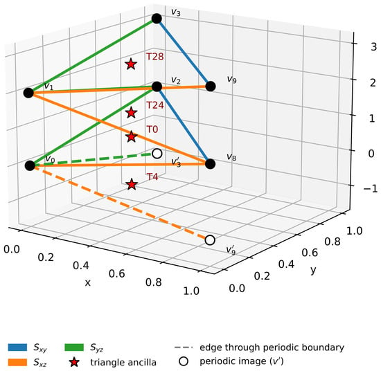
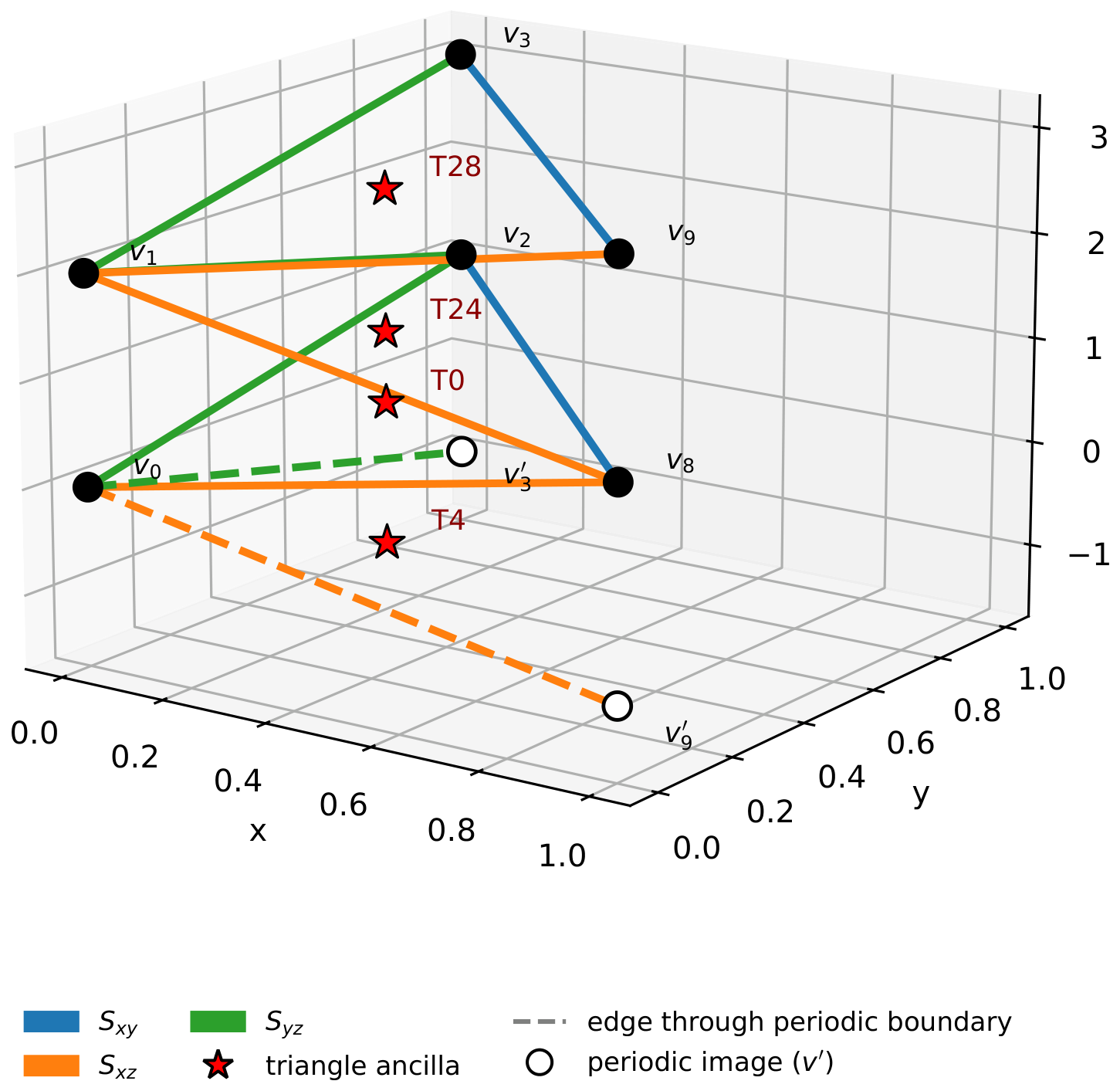
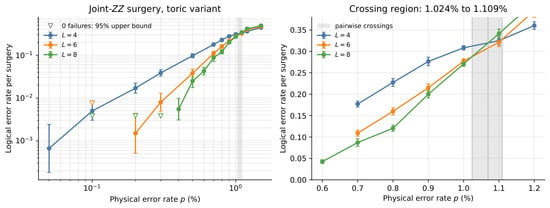
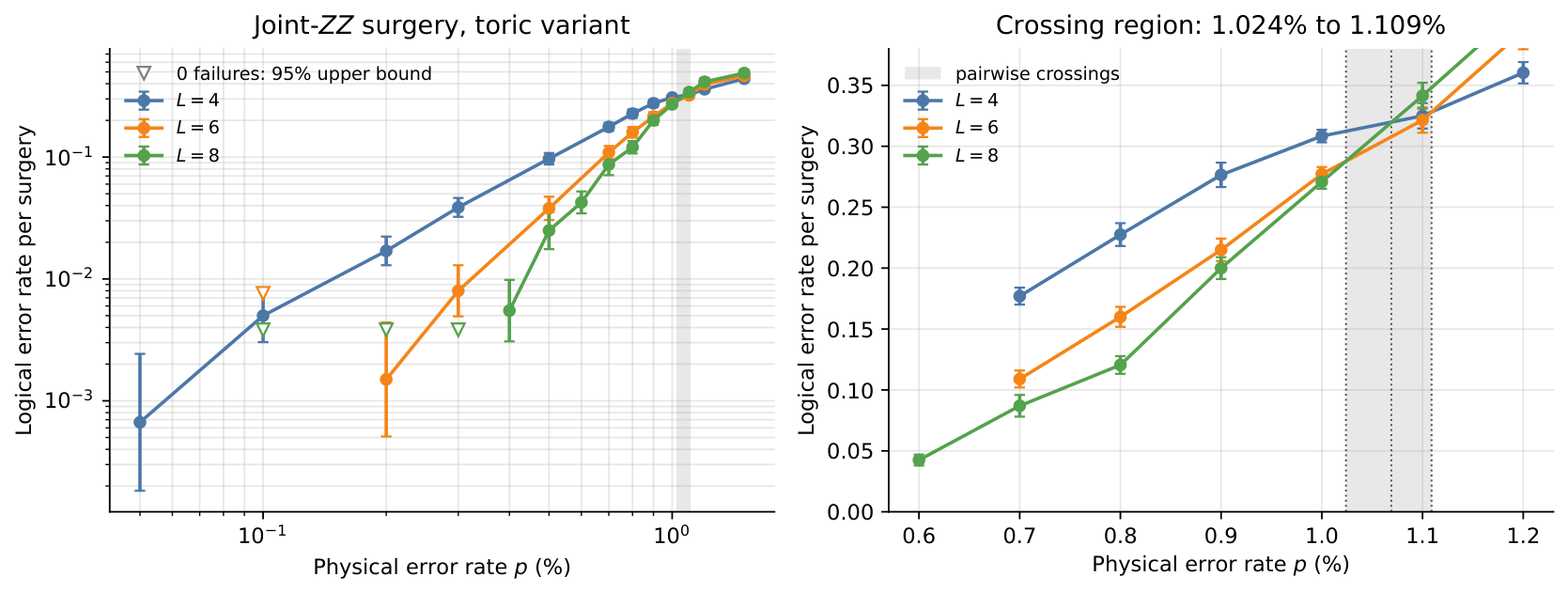
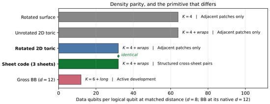
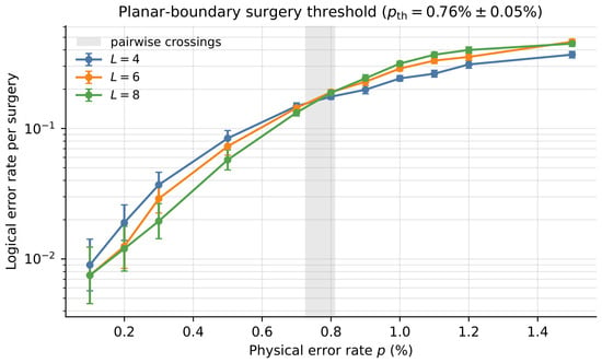
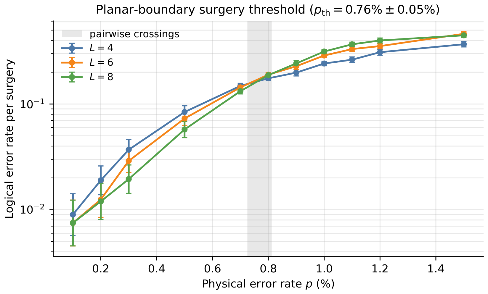
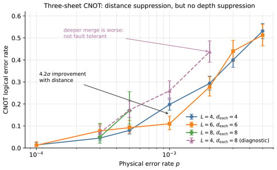
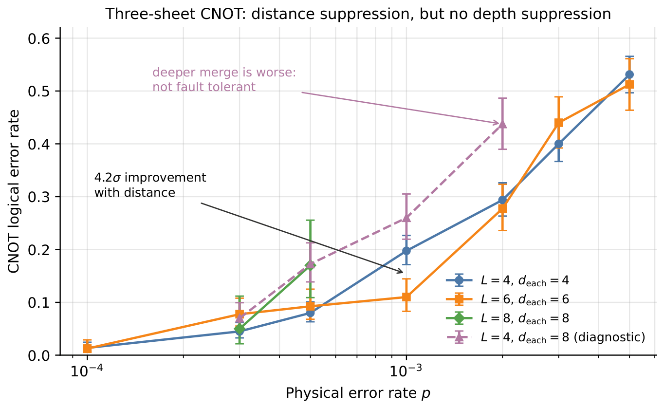

Disclaimer/Publisher’s Note: The statements, opinions and data contained in all publications are solely those of the individual author(s) and contributor(s) and not of MDPI and/or the editor(s). MDPI and/or the editor(s) disclaim responsibility for any injury to people or property resulting from any ideas, methods, instructions or products referred to in the content. |
© 2026 by the author. Licensee MDPI, Basel, Switzerland. This article is an open access article distributed under the terms and conditions of the Creative Commons Attribution (CC BY) license.