Quantum Machine Learning for Water Pollution Profiling in the Rio Santiago Basin

Highlights

What are the main findings?

• A reproducible exploratory pipeline evaluates PCA, a classical RBF kernel, a simulated quantum kernel, and Qiskit hardware quantum-kernel executions for Rio Santiago water-quality records.
• Four IBM Quantum hardware executions were archived: cleaned-data and raw reconstructed-data 24-sample runs, plus two matched 8-record clean/raw consistency checks under job IDs d89sqhlg7okc73ep3q70 and d8a7le8p0eas73dpgog0.

What are the implications of the main findings?

• Quantum feature extraction may provide a useful nonlinear representation for environmental profiling, but current results are hypothesis-generating and must be interpreted against strong classical baselines.
• The manuscript now includes UMAP/HDBSCAN baselines and strict matched-sample controls at n = 8 for PCA, RBF, simulated quantum, and hardware kernels, and at n = 650 for PCA, RBF, and simulated quantum kernels.

Abstract

The Rio Santiago basin is one of the most environmentally stressed river systems in Mexico, with persistent organic, nutrient, microbial, surfactant, and metal contamination. This study develops a near-term quantum machine learning workflow for environmental monitoring and water-pollution profiling using multivariate records from 13 stations between 2009 and 2022. QML is evaluated here because quantum feature maps can define nonlinear, interaction-rich kernels that remain executable on present quantum hardware, providing an alternative representation to compare with classical PCA, RBF, UMAP, and HDBSCAN baselines rather than a presumed computational advantage. After quality screening, log transformation, standardization, and domain-guided feature selection, pollution profiles are evaluated across PCA, RBF spectral clustering, UMAP/KMeans, UMAP/HDBSCAN, a simulated ZZ-style quantum feature-map kernel, and Qiskit Runtime hardware evaluations of the same kernel concept. The initial cleaned-data results show that classical PCA clustering identifies broad lower-load, high organic/surfactant, and rain-season solids/microbial profiles. UMAP/HDBSCAN provides the strongest cleaned full-sample nonlinear baseline, with a silhouette score of 0.568 after excluding 177 noise samples. The simulated quantum-kernel representation separates station-linked gradients, while matched n = 650 stability diagnostics show near-identical quantum-kernel clustering across random initializations (mean ARI = 0.994 for cleaned data) but retain the RBF kernel as the strongest nonlinear comparator. Two 24-sample Qiskit hardware runs and two matched 8-record hardware checks provide proof-of-execution evidence. The analysis is framed as a controlled representation study, not as a claim of quantum advantage.

1. Introduction

Water-quality monitoring programs increasingly generate multivariate datasets whose environmental meaning depends on interactions among organic load, nutrients, solids, microbial indicators, metals, hydrological seasonality, and station location. Conventional single-parameter exceedance analysis remains essential for regulatory assessment, but it can obscure recurring pollution profiles that emerge only when variables are evaluated jointly. This limitation is especially relevant in highly stressed river basins, where contamination sources are heterogeneous and downstream effects accumulate through time. Accordingly, the study is positioned across quantum-computing implementation and algorithmic foundations [1,2,3,4], water-quality artificial-intelligence and Rio Santiago environmental context [5,6,7], time-series, wastewater-monitoring, source-data, toxicology, and regulatory references [8,9,10,11,12], dimensionality-reduction and clustering methods [13,14], regional industrialization and water-quality machine-learning/QML applications [15,16,17,18,19], quantum machine-learning, kernel, variational, NISQ, and quantum-kernel-PCA literature [20,21,22,23,24,25,26], and transferability, remote-sensing, climate-clustering, and WQI comparison studies [27,28,29,30,31].

The Rio Santiago basin offers a compelling case for exploratory multivariate profiling because environmental stress in Mexico and local remediation concerns both point to the need for integrated water-quality analysis [6,7]. Recent work on the Santiago-Guadalajara river basin has also emphasized the relevance of surface-water metal assessment in this regional system [26]. The available monitoring data span 13 stations from 2009 to 2022 and include indicators of organic pollution, surfactants, nutrients, suspended material, conductivity, turbidity, fecal contamination, and selected metals. The central question is not only whether samples exceed individual thresholds, but whether recurring combinations of pollutants define interpretable environmental states across stations and seasons.

Machine learning methods can support this task by learning latent representations before clustering, and recent water-quality studies show that regression, classification, remote-sensing, and sensor-enabled frameworks are increasingly used to predict water-quality indices, classes, and physicochemical parameters [16,17,29]. Linear baselines such as principal component analysis (PCA) provide transparent dimensionality reduction, whereas kernel methods can capture nonlinear similarity patterns. Quantum machine learning extends this idea by embedding classical observations into quantum feature spaces, where inner products define data-dependent kernels [20,21,22,23]. Near-term QML research emphasizes feature maps, kernels, variational circuits, and noisy intermediate-scale quantum algorithms rather than fault-tolerant speedups [21,24,25,26]. In environmental applications, this approach is still early-stage, but recent studies have begun to test quantum support vector classifiers, quantum neural networks, and quanvolutional preprocessing for water-quality and turbidity prediction [18,19]. Rigorous framing is therefore needed to avoid overstating computational advantage while still evaluating whether quantum encodings can add useful environmental representations.

This paper has four objectives: (1) develop a reproducible QML workflow for multivariate Rio Santiago water-quality records; (2) compare the induced quantum-kernel profiles with classical PCA, RBF, UMAP, and HDBSCAN baselines; (3) evaluate whether the resulting clusters correspond to interpretable station, season, pollutant, and exceedance signatures; and (4) test how cleaned versus raw reconstructed data layers alter the learned similarity geometry. Unlike supervised water-quality prediction studies that forecast water-quality index, class labels, or turbidity [17,18,19,29], the present work focuses on unsupervised pollution-profile discovery in a multistation river-monitoring archive. The contribution is a reproducible analysis scaffold, an initial environmental interpretation of the learned profiles, and a set of methodological caveats that define the next experimental iteration.

The method is potentially transferable to other hydraulic environments, including lakes, groundwater systems, reservoirs, and coastal aquifers, but only after adapting the feature set, hydrological context, sampling design, and validation data to each system. For example, groundwater contamination studies often require hydrogeochemical and salinity-intrusion variables that are not central to this surface-river dataset [27]. The present article should therefore be read as a Rio Santiago case study and a transferable workflow template, not as a universal water-quality index or final source-apportionment model.

2. Materials and Methods

2.1. Study Area

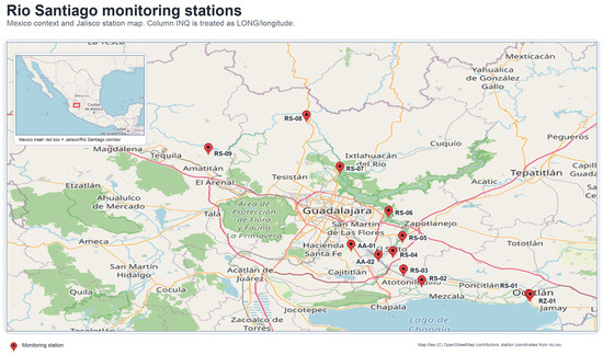
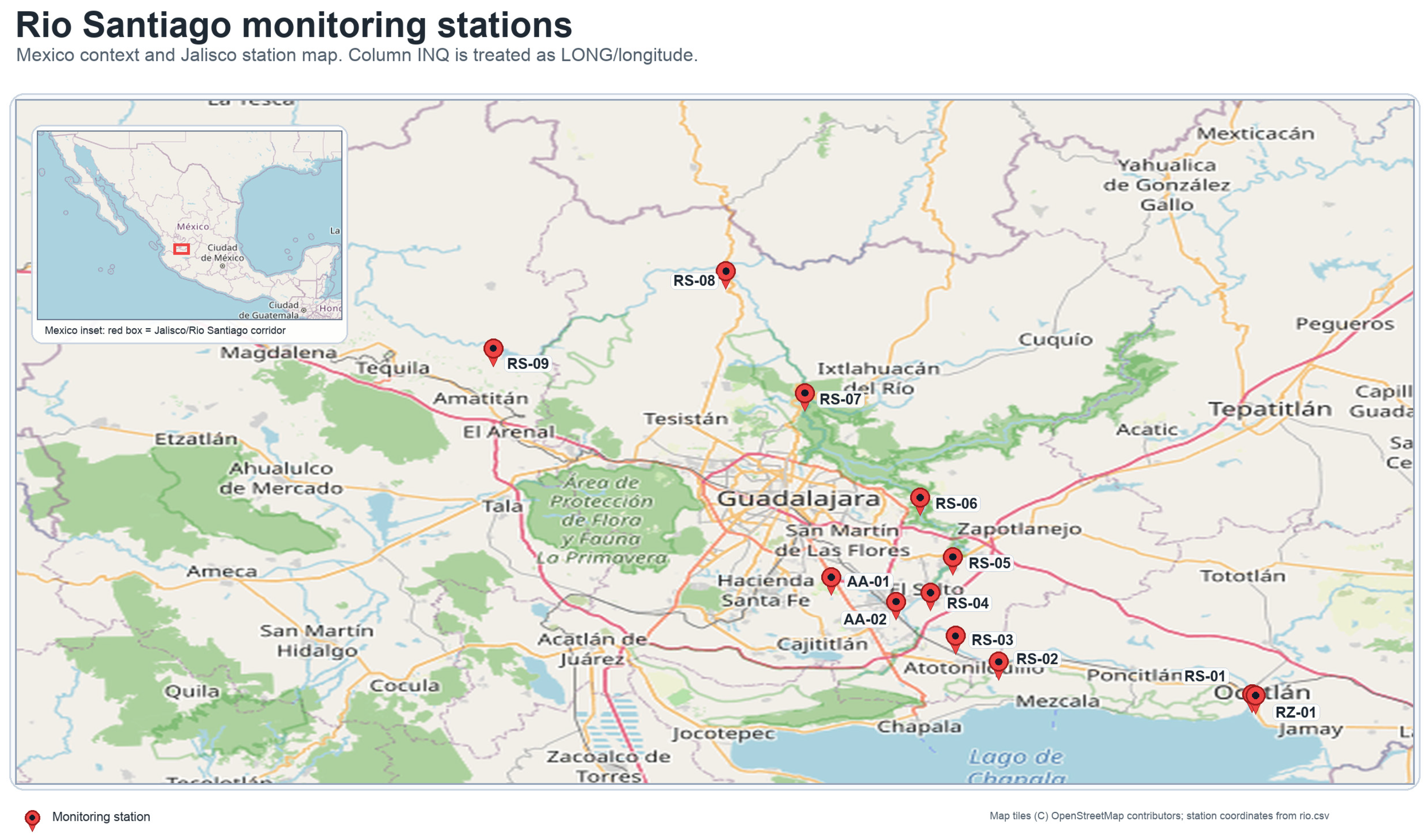
The study area is the Rio Santiago monitoring corridor represented in the HidroHack archive. The ‘rio.csv’ file includes georeferenced monitoring stations through the ‘EST’, ‘LAT’, and ‘INQ’ fields. Because ‘INQ’ is not a standard geographic abbreviation and its values are negative coordinates in the expected Jalisco longitude range, it is treated here as the longitude field, likely corresponding to ‘LONG’ in the original coordinate schema. The 13 points include ten Rio Santiago stations from Ocotlán (RS-01) through Paso La Yesca (RS-10), two tributary or adjacent-system stations associated with the Chapala-airport and El Muelle areas (AA-01 and AA-02), and one Rio Zula station (RZ-01). The station descriptions identify key locations such as Presa Corona, Ex-hacienda de Zapotlanejo, Salto-Juanacatlán, Puente Grande, Matatlán, Paso de Guadalupe, San Cristóbal de la Barranca, Camino al Salvador-Tequila, and Paso La Yesca. The coordinate table spans approximately 20.34–21.19 degrees N and 102.77–104.07 degrees W, following the river from upstream and metropolitan-influenced reaches toward downstream sections. Figure 1 shows the resulting station map used for spatial orientation.

Figure 1. Rio Santiago monitoring corridor. The map shows the 13 georeferenced monitoring stations used to orient pollution-profile interpretation. It is an original figure produced by the authors; it supports spatial interpretation but is not a formal source-apportionment map because source-type, discharge-volume, flow, and land-use layers were not available in the analysis archive.

This spatial setting matters because the Santiago system integrates multiple pressure types. Prior regional work describes the basin as affected by industrialization and environmental-health concerns [15], and recent Santiago-Guadalajara evidence reinforces the importance of monitoring heavy metals in surface waters [26]. In the present analysis, station-level profiles are therefore interpreted as integrated monitoring signatures that may reflect mixtures of municipal wastewater, industrial effluents, agro-industrial inputs, livestock or agricultural runoff, landfill influence, and storm-driven solids transport. The data available here provide georeferenced monitoring-station coordinates, but not source-type classifications, discharge volumes, flow measurements, or land-use layers; therefore, the map supports spatial orientation and hypothesis generation rather than formal source apportionment.

2.2. Study Data

The working analysis uses a cleaned wide table containing 1970 water-quality records from 13 Rio Santiago monitoring stations, with sampling dates ranging from 10 February 2009 to 5 July 2022. The data source is associated with the HidroHack 2023 water-data initiative [10]. The project archive also includes the apparent raw long-form source table, parameter lookup table, and monitoring-point lookup table. A reproducible reconstruction script pivots the raw long-form measurements into a station-date wide table and confirms that the cleaned HidroHack file is a processed analysis layer rather than a direct raw pivot. The raw reconstruction preserves the same 1970 station-date keys but matches only 51.5% of comparable cells exactly, indicating that cleaning, imputation, censoring, or formatting decisions materially affect the analysis layer. The selected variables include SAAM, biochemical oxygen demand, chemical oxygen demand, nitrogen species, phosphorus, solids, conductivity, turbidity, fecal coliforms, and selected metals. Sampling dates were parsed to derive year, month, and season indicators so that pollutant profiles could be interpreted against temporal and hydrological context.

2.3. Preprocessing and Quality Flags

The current pipeline treats the source file as a processed monitoring dataset rather than pristine raw laboratory data. Domain-relevant water-quality variables were selected, skewed concentration variables were log-transformed, and all modeling features were standardized. Repeated or censoring-like values and known consistency issues were flagged for interpretation instead of being removed at this stage. Exceedance features were interpreted against available water-quality thresholds and Mexican drinking-water quality standards where applicable [12]. This conservative choice preserves sample size while making data-quality limitations visible in the cluster summaries. Water-quality indices (WQIs) are a complementary integration strategy for translating multiple parameters into management-oriented scores, and prior surface-water work has combined seasonal monitoring, PCA, and WQI calculation [30]; the present study instead uses unsupervised clustering to identify recurring pollution profiles before assigning a single index value.

2.4. Classical Baselines

Classical baselines include PCA/KMeans, RBF spectral clustering, UMAP/KMeans, and UMAP/HDBSCAN. PCA features were computed by singular-value decomposition and clustered with KMeans. A nonlinear radial-basis-function similarity matrix was also constructed and clustered by spectral clustering. UMAP was run with n_neighbors = 30, min_dist = 0.05, and random_state = 20260525; KMeans was evaluated for k = 3, 4, and 5 in the two-dimensional UMAP embedding, and HDBSCAN used min_cluster_size = 25 and min_samples = 10 [13,14]. Cluster quality was summarized using silhouette and Davies-Bouldin scores in the relevant evaluation space, and profile interpretation used pollutant medians, station composition, seasonal composition, quality flags, and exceedance rates, following the broader logic of wastewater and environmental monitoring studies that combine temporal, spatial, and compositional evidence [9].

2.5. Quantum Feature-Map Kernel

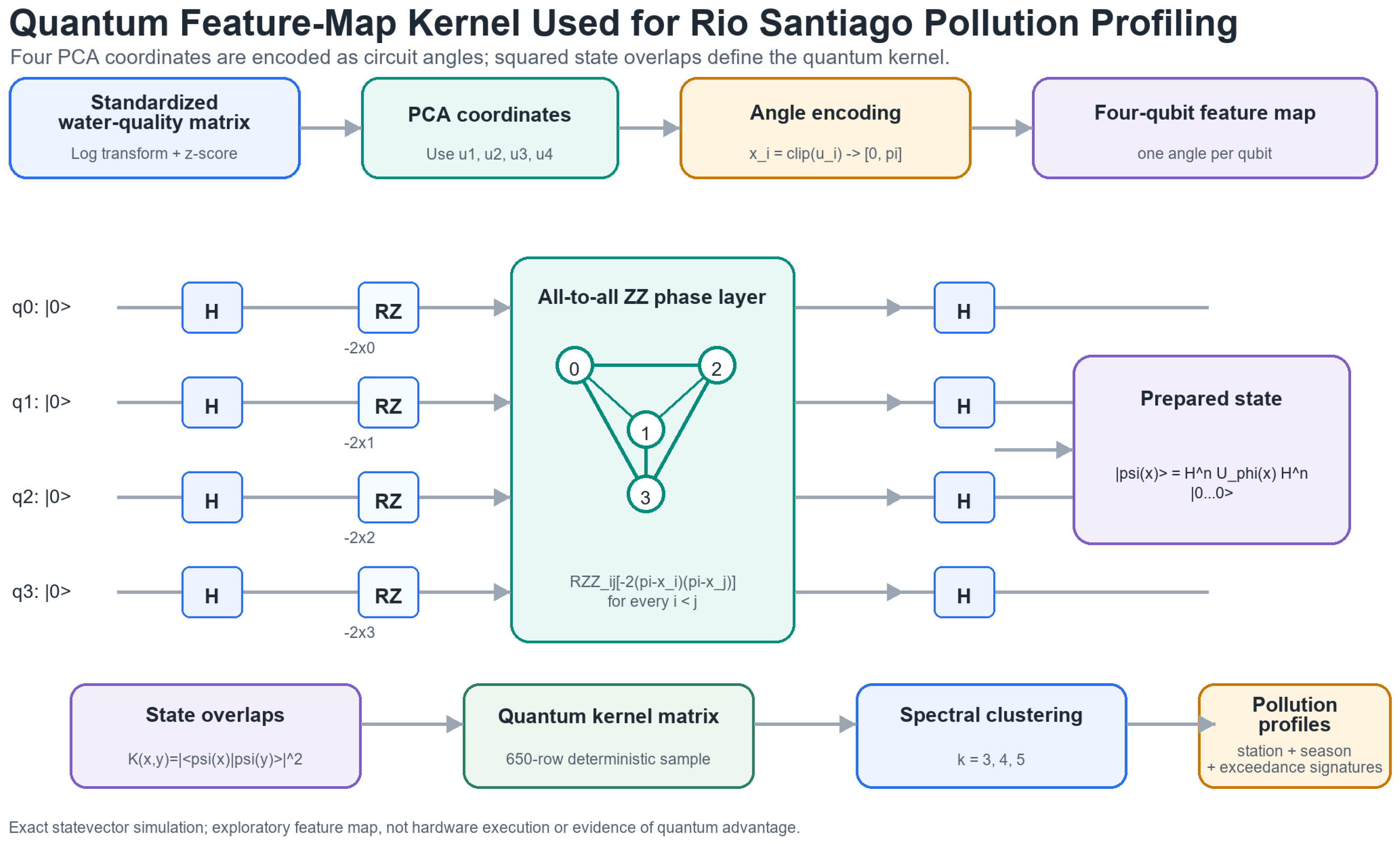
The quantum machine learning path uses an exact statevector simulation of a four-qubit ZZ-style feature map. The input to the circuit is not the raw pollutant vector; instead, the first four PCA scores are used as compact, decorrelated coordinates of the standardized monitoring matrix. Each coordinate is clipped to the interval [−3, 3] and linearly rescaled to an angle in [0, pi]. This produces an encoded vector x = (x1, x2, x3, x4), with one angle assigned to each qubit. This follows the quantum-kernel view of QML, in which the data encoding circuit defines the effective feature space and therefore the learned similarity measure [21,22,23].

The ZZ map was selected as a compact exploratory encoding because its pairwise phase terms create an explicit second-order interaction structure among PCA coordinates while keeping circuit width and depth feasible for current public hardware access. This choice should be understood as a hypothesis about nonlinear representation, not as a theoretically proven optimal Hilbert-space embedding for pollutant chemistry. Alternative Pauli feature maps, different entanglement patterns, and advanced classical kernels remain necessary controls for a mature comparison.

For an encoded observation x, the circuit starts from |0000>, applies Hadamard gates to all qubits, applies data-dependent single-qubit Z phases, applies all-to-all pairwise ZZ phases, and finishes with a second Hadamard layer. In statevector form, the diagonal phase applied between the two Hadamard layers is exp(i[sum_i x_i z_i + sum_{i<j}(pi–x_i)(pi–x_j)z_i z_j]), where z_i is the Pauli-Z eigenvalue of qubit i. The six pairwise interactions are therefore applied to qubit pairs (0, 1), (0, 2), (0, 3), (1, 2), (1, 3), and (2, 3).

Under the common gate convention RZ(theta) = exp(-i theta Z/2) and RZZ(theta) = exp(-i theta ZiZj/2), the same feature map can be implemented with RZ_i(-2x_i) gates and RZZ_ij(-2(pi–x_i)(pi–x_j)) gates. Pairwise sample similarity is then defined by the squared state overlap K(x, y) = |<psi(x)|psi(y)>|^2, yielding a quantum kernel matrix for spectral clustering. The simulator implementation remains intentionally transparent; the subsequent Qiskit Runtime run tests the same kernel concept on hardware within the constraints of current NISQ devices [24,25].

2.6. Representation Geometry and Environmental Rationale

The ZZ feature map was used because it induces a similarity geometry that is neither purely linear in the PCA coordinates nor identical to the radial-basis-function baseline. After the first Hadamard layer, each computational-basis component receives a data-dependent phase. The single-qubit Z terms encode the signed position of a sample along each principal pollution axis, while the pairwise ZZ terms encode products between axes. When two samples are compared through squared state overlap, samples remain similar only when their induced phase patterns agree across both marginal coordinates and second-order coordinate interactions. This is the operational advantage tested here: QML provides a hardware-executable nonlinear kernel whose interaction structure can be compared directly with transparent classical baselines.

This geometry is relevant for water-quality profiling because environmental states are rarely defined by one pollutant in isolation. Organic load, surfactants, nitrogen species, solids, turbidity, conductivity, microbial indicators, and metals can co-vary through shared hydrological conditions, treatment failures, industrial inputs, urban runoff, or downstream accumulation. A linear PCA representation can identify dominant axes of variation, but it may collapse samples with different interaction signatures onto nearby coordinates. The ZZ map deliberately asks whether combinations of these compact axes create a different neighborhood structure.

The use of PCA scores before the quantum map is therefore not only a dimensionality reduction convenience; it also defines four orthogonal environmental coordinates that summarize the standardized monitoring matrix before nonlinear encoding. This design is distinct from full quantum kernel PCA algorithms, which seek to diagonalize or approximate kernel matrices directly on quantum hardware and can have favorable query complexity only under specific data-access and dimensionality assumptions [26]. In the present environmental workflow, PCA is used as a transparent classical compression step, and the quantum kernel then acts on this compact representation by phase-wrapping the coordinates and their pairwise interactions. In practical terms, two observations with similar overall organic burden but different solids-microbial or nutrient-metal coupling may receive a different quantum similarity than they would under a simple Euclidean or RBF geometry.

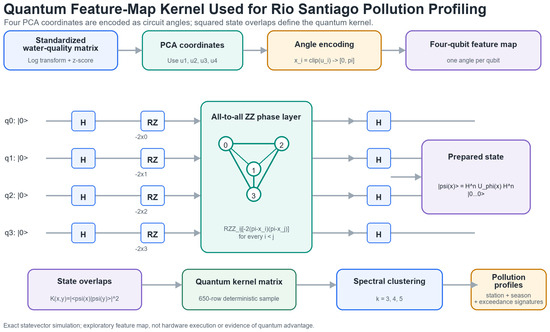
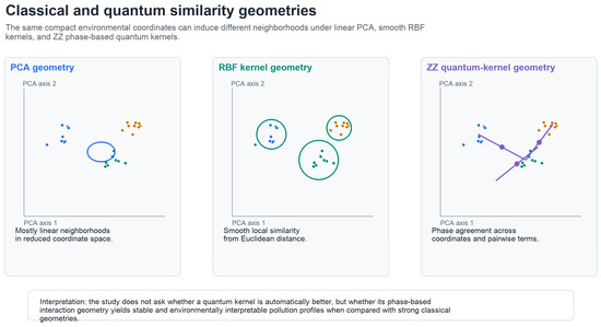
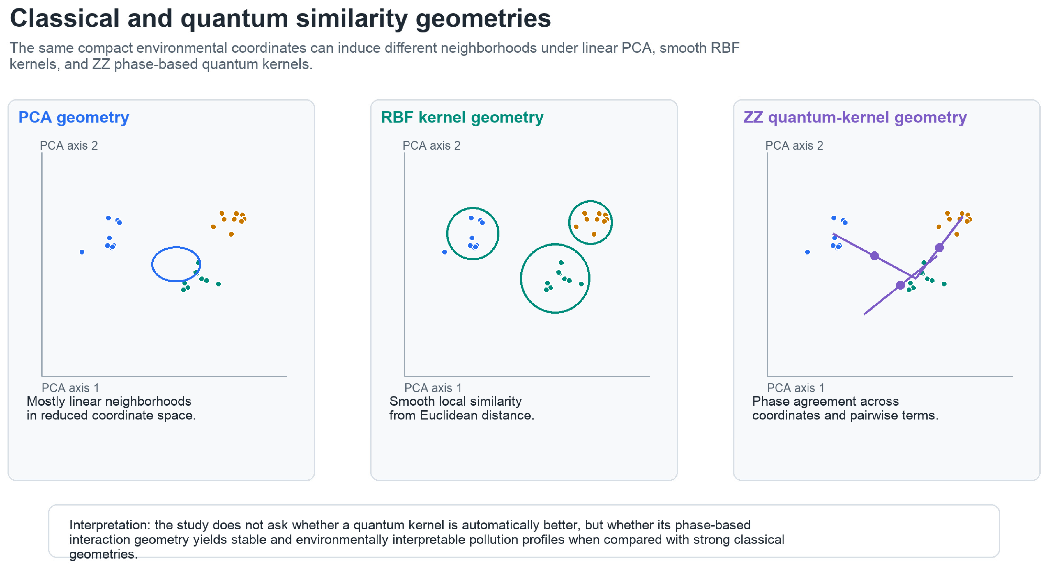
This rationale remains exploratory. The present feature map is not claimed to be optimal for pollutant chemistry, and the matched n = 650 results show that the classical RBF kernel is still the strongest nonlinear comparator. The value of the ZZ map in this study is methodological: it provides a controlled, hardware-executable representation whose induced kernel can be inspected, compared with classical geometries, and interpreted through station, season, pollutant median, and exceedance signatures. Figure 2 summarizes the implemented feature-map circuit. Figure 3 compares the corresponding similarity geometries.

Figure 2. Author-produced schematic visualization of the quantum feature-map kernel used for Rio Santiago pollution profiling. Standardized water-quality measurements are reduced to four PCA coordinates, clipped and rescaled to circuit angles, encoded in a four-qubit ZZ-style feature map, and compared through squared statevector overlaps to form the quantum kernel used for spectral clustering. This schematic is provided to document the implemented computational workflow and is not an experimental image.

Figure 3. Author-produced conceptual visualization comparing the similarity geometries evaluated in the study. PCA neighborhoods are primarily linear and distance-based in reduced coordinates, RBF neighborhoods decay smoothly with local Euclidean distance, and the ZZ quantum kernel compares phase patterns induced by both coordinates and pairwise interaction terms. The figure is intended to clarify the representation question rather than report an additional experiment or experimental image.

2.7. Qiskit Hardware Execution

After the simulator-based scaffold was established, a standalone Qiskit version of the pipeline was executed through IBM Quantum Runtime. The hardware path uses QiskitRuntimeService and EstimatorV2 to estimate pairwise kernel entries as zero-projector expectation values for U(y)^dagger U(x), where U is the four-qubit feature-map circuit. To keep the hardware experiment tractable under queue and circuit-count constraints, the kernel was first evaluated on deterministic 24-sample subsets. The cleaned-data run selected IBM Quantum backend ibm_kingston and produced job ID d89r862s46sc73fb0acg. A second run on the raw reconstructed table used the same backend and produced job ID d89s621789is7393nh1g.

Two matched consistency checks were added. Both used the same eight station-date rows in the cleaned HidroHack and raw reconstructed tables, with matched positions 9, 267, 843, 1263, 1673, 1860, 1906, and 1951. The first matched job ran on backend ibm_kingston under job ID d89sqhlg7okc73ep3q70; the second ran on backend ibm_marrakesh under job ID d8a7le8p0eas73dpgog0. Each submitted 72 circuits and directly addresses the sampling-asymmetry criticism by holding row membership fixed across the cleaned and raw data views.

The hardware runs should be interpreted as proof-of-execution and methodological bridges from the simulator scaffold to Qiskit infrastructure. They confirm that the feature-map kernel can be submitted to real IBM Quantum hardware, while model selection remains based on the larger simulator and classical controls.

2.8. Validation and Interpretation

The principal validation goal of this phase is interpretability rather than a single global ranking. Clusters were evaluated numerically and then profiled by station, season, pollutant medians, and exceedance signatures. Silhouette and Davies-Bouldin scores are sensitive to sample size, evaluation space, and cluster balance; therefore, PCA4, UMAP2, quantum spectral, and hardware quantum metrics are interpreted within method families unless matched controls are explicitly used. The raw reconstructed dataset was used as a sensitivity analysis rather than as a replacement for the cleaned analysis layer.

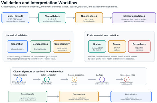
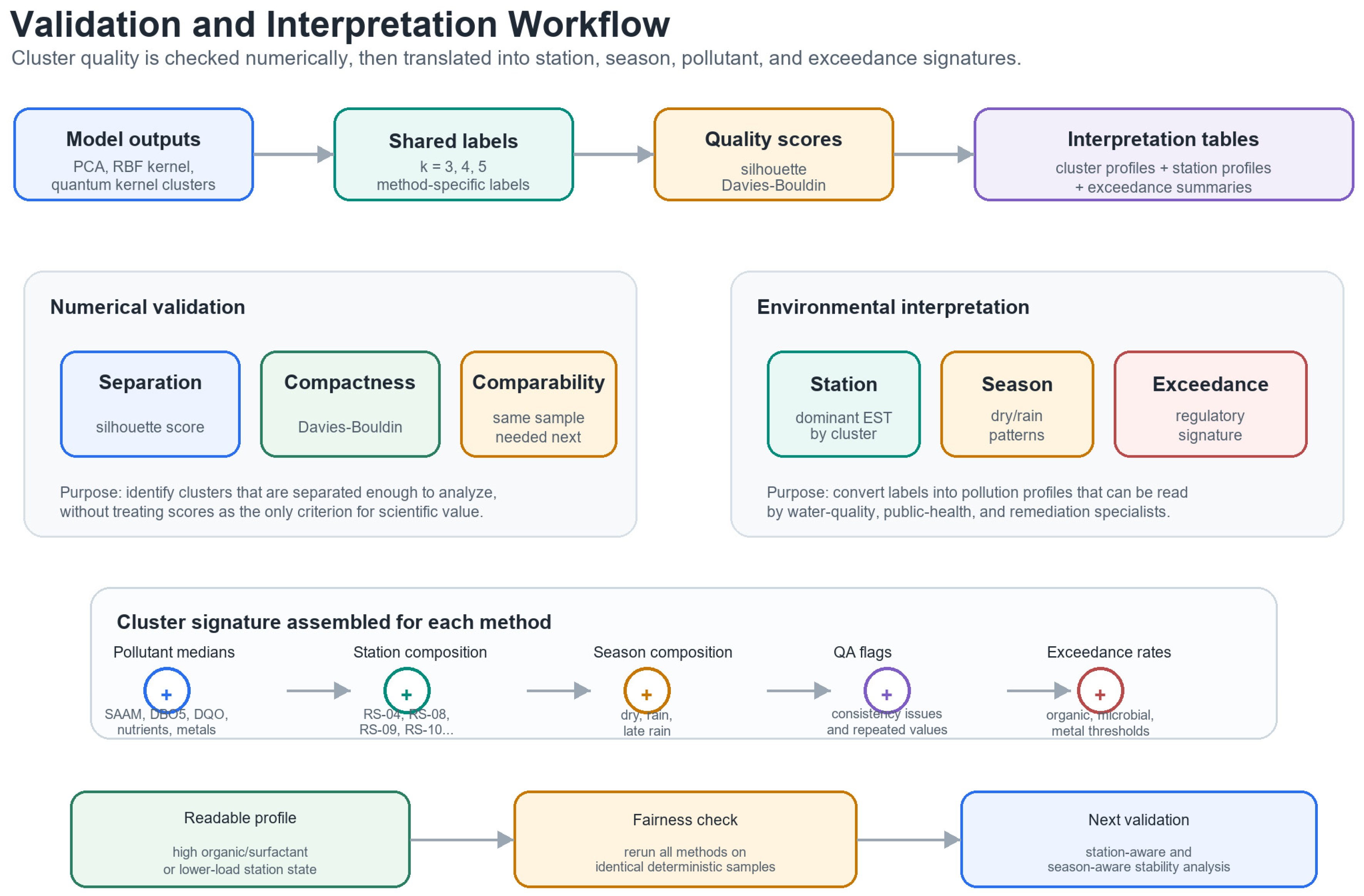
To reduce sample-size bias, strict matched-sample controls were added. The n = 8 control uses the same hardware-executed station-date rows for PCA, RBF spectral clustering, the simulated quantum kernel, and the Qiskit hardware kernel. The n = 650 control uses an identical intermediate sample for PCA, RBF spectral clustering, and the simulated quantum kernel in both cleaned and raw reconstructed data views. These controls define the most comparable numerical results in the paper. Figure 4 summarizes this validation and interpretation workflow.

Figure 4. Author-produced workflow visualization used to translate clustering outputs into environmentally meaningful pollution profiles. Numerical scores summarize separation and compactness, while station composition, seasonal structure, pollutant medians, quality flags, and exceedance rates provide the environmental signature of each cluster. This schematic documents the analysis procedure and is not an experimental image.

3. Results

3.1. Hierarchical Reading of the Experiments

The results are organized hierarchically to avoid treating every comparison as equally decisive. First, classical geometry defines the main empirical baseline through PCA, RBF kernels, UMAP, and HDBSCAN. Second, the simulated quantum geometry tests whether the ZZ feature-map kernel creates an alternative nonlinear neighborhood structure with interpretable pollution profiles. Third, hardware execution is treated as a feasibility and consistency layer, not as final model selection. Fourth, environmental interpretation translates the learned clusters into station, season, pollutant, and exceedance signatures. This hierarchy keeps the raw reconstruction, n = 8 hardware control, n = 24 hardware runs, and n = 650 simulator controls in their appropriate evidentiary roles.

3.2. Initial Clustering Performance

The first-pass cleaned-data results indicate that both classical and quantum representations produce nonrandom, interpretable structure. PCA followed by KMeans gives the strongest full-sample baseline among the current cleaned classical runs. The simulated quantum-kernel embeddings show coherent structure on a 650-sample subset, and the cleaned-data Qiskit hardware run produced the strongest hardware-subset score at k = 3, with silhouette 0.416 and Davies-Bouldin 0.795 on the hardware quantum embedding. Because these scores are computed in different spaces, they are reported as within-family diagnostics rather than cross-space evidence of superiority. Table 1 summarizes the main cleaned-data and raw reconstructed-data sensitivity results.

Table 1. Primary cleaned-data results and raw reconstructed-data sensitivity results.

Data View	Method	k	n	Evaluation Space	Main Metric
Cleaned HidroHack	PCA + KMeans	3	1970	PCA4	Silhouette = 0.353; DB = 0.988
Cleaned HidroHack	RBF spectral clustering	5	1970	PCA4	Silhouette = 0.245; DB = 1.405
Cleaned HidroHack	UMAP + KMeans	4	1970	UMAP2	Silhouette = 0.486; DB = 0.650
Cleaned HidroHack	UMAP + HDBSCAN	18	1793 clustered	UMAP2	Silhouette = 0.568; DB = 0.399; noise = 177
Cleaned HidroHack	Simulated quantum kernel	3	650	Quantum embedding	Silhouette = 0.372; DB = 0.960
Cleaned HidroHack	Qiskit hardware kernel	3	24	Hardware quantum embedding	Silhouette = 0.416; DB = 0.795
Raw reconstruction	PCA + KMeans	3	1970	PCA4	Silhouette = 0.338; DB = 1.074
Raw reconstruction	RBF spectral clustering	3	1970	PCA4	Silhouette = 0.556; DB = 0.816
Raw reconstruction	UMAP + KMeans	5	1970	UMAP2	Silhouette = 0.541; DB = 0.624
Raw reconstruction	UMAP + HDBSCAN	6	1935 clustered	UMAP2	Silhouette = 0.353; DB = 0.498; noise = 35
Raw reconstruction	Simulated quantum kernel	3	650	Quantum embedding	Silhouette = 0.487; DB = 0.727
Raw reconstruction	Qiskit hardware kernel	5	24	Hardware quantum embedding	Silhouette = 0.438; DB = 0.788
Strict matched n = 8 clean	PCA + KMeans	5	8	PCA4	Silhouette = 0.471; DB = 0.587
Strict matched n = 8 clean	RBF spectral clustering	5	8	PCA4	Silhouette = 0.426; DB = 0.802
Strict matched n = 8 clean	Simulated quantum kernel	5	8	Quantum embedding	Silhouette = 0.427; DB = 0.733
Strict matched n = 8 clean	Qiskit hardware kernel	2	8	Hardware quantum embedding	Silhouette = 0.639; DB = 0.407
Strict matched n = 8 raw	PCA + KMeans	5	8	PCA4	Silhouette = 0.547; DB = 0.587
Strict matched n = 8 raw	RBF spectral clustering	5	8	PCA4	Silhouette = 0.485; DB = 0.605
Strict matched n = 8 raw	Simulated quantum kernel	2	8	Quantum embedding	Silhouette = 0.841; DB = 0.141
Strict matched n = 8 raw	Qiskit hardware kernel	5	8	Hardware quantum embedding	Silhouette = 0.564; DB = 0.559
Strict matched n = 650 clean	PCA + KMeans	3	650	PCA4	Silhouette = 0.337; DB = 1.026
Strict matched n = 650 clean	RBF spectral clustering	2	650	PCA4	Silhouette = 0.613; DB = 0.522
Strict matched n = 650 clean	Simulated quantum kernel	2	650	Quantum embedding	Silhouette = 0.508; DB = 0.713
Strict matched n = 650 raw	PCA + KMeans	5	650	PCA4	Silhouette = 0.334; DB = 0.891
Strict matched n = 650 raw	RBF spectral clustering	2	650	PCA4	Silhouette = 0.659; DB = 0.491
Strict matched n = 650 raw	Simulated quantum kernel	2	650	Quantum embedding	Silhouette = 0.607; DB = 0.650

Note: only the strongest or most representative setting for each method family is shown. Metrics are reported within their native evaluation spaces, so UMAP2, PCA4, quantum spectral embeddings, and hardware quantum embeddings should not be interpreted as a single homogeneous leaderboard. HDBSCAN reports clustered samples after excluding noise. The strict matched n = 8 rows use the same eight station-date records for PCA, RBF, simulated quantum, and Qiskit hardware. The strict matched n = 650 rows use the same 650 station-date records for PCA, RBF, and simulated quantum comparisons; hardware is not feasible at this size in the present resource budget. Hardware job IDs are d89r862s46sc73fb0acg, d89s621789is7393nh1g, d89sqhlg7okc73ep3q70, and d8a7le8p0eas73dpgog0.

3.3. Stability Diagnostics

To add a statistical robustness check, the strict matched n = 650 control was re-evaluated with seed and subsampling diagnostics. For each primary method family, 20 KMeans initializations were compared using pairwise adjusted Rand index (ARI), and silhouette variability was estimated across 50 deterministic 80% subsamples. These diagnostics do not replace external validation, but they test whether the reported geometries are numerically fragile.

The cleaned-data RBF k = 2 solution was perfectly stable across seeds (mean ARI = 1.000), while the cleaned simulated quantum k = 2 solution was nearly identical across seeds (mean ARI = 0.994). Their subsample silhouette intervals were also coherent: 0.518–0.657 for RBF and 0.497–0.516 for the simulated quantum kernel. PCA_KMeans_k3 was less stable (mean ARI = 0.816), consistent with its weaker separation. In the raw reconstructed view, RBF k = 2 and simulated quantum k = 2 were both seed-stable (mean ARI = 1.000), whereas PCA_KMeans_k5 was less stable (mean ARI = 0.651).

These stability results sharpen rather than weaken the cautious interpretation. They show that the main nonlinear geometries are not artifacts of a single random initialization, but they also confirm that the strongest and most stable comparator remains the classical RBF kernel. The simulated quantum kernel is therefore best read as a stable alternative representation with environmental interpretability, not as a superior clustering method under the present feature map. Table 2 reports these stability diagnostics for the strict matched n = 650 control.

Table 2. Stability diagnostics for the strict matched n = 650 control.

Data View	Method	k	Seed ARI Mean	Silhouette Mean	Silhouette 5–95%
Cleaned HidroHack	PCA + KMeans	3	0.816	0.342	0.335–0.351
Cleaned HidroHack	RBF spectral clustering	2	1.000	0.601	0.518–0.657
Cleaned HidroHack	Simulated quantum kernel	2	0.994	0.506	0.497–0.516
Raw reconstruction	PCA + KMeans	5	0.651	0.327	0.318–0.337
Raw reconstruction	RBF spectral clustering	2	1.000	0.648	0.559–0.706
Raw reconstruction	Simulated quantum kernel	2	1.000	0.605	0.594–0.619

Note: seed stability is summarized by the mean pairwise adjusted Rand index (ARI) across 20 KMeans initializations. Silhouette variability is summarized across 50 deterministic 80% subsamples using the same matched n = 650 row set. These diagnostics test numerical robustness of the current clustering geometry; they do not establish external environmental validity.

3.4. Raw Reconstructed Data Sensitivity Analysis

The apparent raw long-form table was also reconstructed into a station-date wide table and passed through the same classical, simulated quantum, and Qiskit hardware workflows. Because this table does not reproduce the cleaned HidroHack values exactly, the resulting scores are treated as sensitivity evidence. The raw reconstructed view changes the metric landscape: RBF_Spectral_k3 becomes the strongest full-sample classical baseline on PCA4, with silhouette 0.556 and Davies-Bouldin 0.816. The simulated raw quantum-kernel run gives its strongest result at k = 3, with silhouette 0.487 and Davies-Bouldin 0.727 on the quantum embedding. The raw Qiskit hardware execution gives its strongest 24-sample result at k = 5, with silhouette 0.438 and Davies-Bouldin 0.788.

The modern nonlinear classical baselines sharpen this comparison. In the cleaned HidroHack view, UMAP_HDBSCAN identified 18 clusters among 1793 clustered samples, with 177 samples treated as noise, and achieved silhouette 0.568 and Davies-Bouldin 0.399 in the UMAP embedding. UMAP_KMeans_k4 was the strongest fixed-k UMAP baseline for the cleaned view, with silhouette 0.486 and Davies-Bouldin 0.650. In the raw reconstructed view, UMAP_KMeans_k5 achieved silhouette 0.541 and Davies-Bouldin 0.624, while UMAP_HDBSCAN identified 6 clusters among 1935 clustered samples with silhouette 0.353 and Davies-Bouldin 0.498. These results confirm that modern nonlinear classical baselines are competitive and must remain central comparators.

These shifts reinforce the importance of documenting the data layer. The quantum and nonlinear classical representations remain environmentally structured under the raw reconstruction, but the preferred k and relative baselines differ from the cleaned-data analysis. This supports reporting the raw reconstruction as a robustness check while retaining the cleaned HidroHack table as the primary analysis dataset.

3.5. Matched Hardware Consistency Check

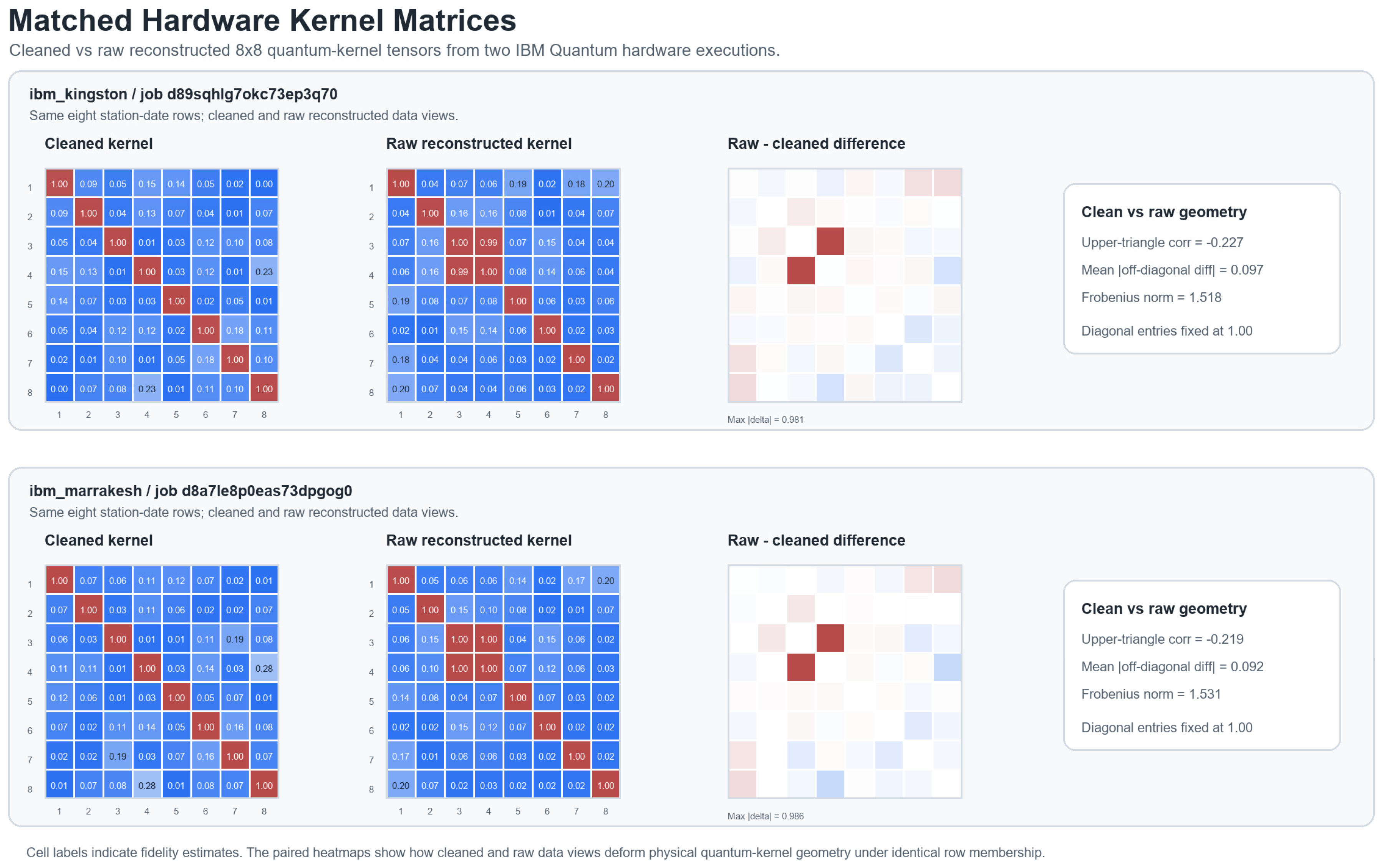
The matched 8-record Qiskit runs provide the most controlled hardware comparison in the current analysis because cleaned and raw reconstructed kernels use identical station-date rows. The sampled records correspond to matched positions 9, 267, 843, 1263, 1673, 1860, 1906, and 1951, spanning stations RS-08, RS-06, RS-09, RS-10, RS-03, and RS-07 between 2009 and 2022. On ibm_marrakesh, the cleaned-data hardware kernel gives its strongest result at k = 2, with silhouette 0.639 and Davies-Bouldin 0.407, while the raw reconstructed hardware kernel gives its strongest result at k = 5, with silhouette 0.564 and Davies-Bouldin 0.559. The ibm_kingston replicate gives the same preferred cleaned-data granularity (k = 2, silhouette 0.733) and a similar raw optimum (k = 5, silhouette 0.537).

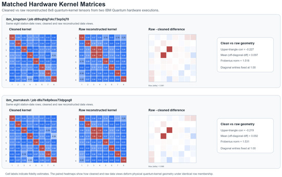
The matched hardware kernels also differ geometrically. On ibm_marrakesh, the upper-triangle correlation between cleaned and raw kernel entries is –0.219, with a mean absolute off-diagonal difference of 0.092 and a Frobenius norm difference of 1.531. The ibm_kingston replicate is similar: correlation = –0.227, mean absolute off-diagonal difference = 0.097, and Frobenius norm difference = 1.518. These values strengthen the central data-lineage conclusion: cleaned and raw reconstructed data layers can produce meaningfully different quantum-kernel geometries even when row membership is held fixed.

When PCA, RBF, simulated quantum, and hardware kernels are all evaluated on this same n = 8 subset, the strongest cleaned-data results are Qiskit hardware k = 2 (silhouette score = 0.639), PCA k = 5 (0.471), simulated quantum k = 5 (0.427), and RBF k = 5 (0.426). In the raw reconstructed view, the strongest n = 8 results are simulated quantum k = 2 (0.841), Qiskit hardware k = 5 (0.564), PCA k = 5 (0.547), and RBF k = 5 (0.485). These values are retained as a strict row-membership control, not as a model-selection basis.

The intermediate n = 650 matched control gives a more stable non-hardware comparison. In the cleaned-data view, RBF_Spectral_k2 gives a silhouette score of 0.613, simulated quantum k = 2 gives 0.508, and PCA_KMeans_k3 gives 0.337. In the raw reconstructed view, RBF_Spectral_k2 gives 0.659, simulated quantum k = 2 gives 0.607, and PCA_KMeans_k5 gives 0.334. Thus, under the current matched n = 650 control, the RBF kernel remains the strongest classical nonlinear comparator and must be treated as a serious baseline for any future quantum-kernel claim.

This n = 650 result is important because it defines the immediate methodological target for future quantum feature engineering. To compete with the RBF baseline, future quantum kernels should explore feature maps that alter the similarity geometry more deliberately than the present compact ZZ map, including trainable data re-uploading layers, alternative Pauli encodings, non-all-to-all entanglement patterns aligned with pollutant groups, or hybrid kernels that combine station/season context with concentration features. Without such controls, the current RBF result remains the more parsimonious nonlinear explanation. Figure 5 visualizes the matched hardware kernels used in this comparison.

Figure 5. Matched hardware quantum-kernel matrices for the same eight station-date rows in the cleaned HidroHack and raw reconstructed data views. The heatmaps contrast cleaned and raw reconstructed 8 × 8 hardware fidelity matrices for ibm_kingston (job d89sqhlg7okc73ep3q70) and ibm_marrakesh (job d8a7le8p0eas73dpgog0), with difference panels summarizing how the raw reconstruction changes off-diagonal kernel structure.

3.6. Classical Pollution Profiles

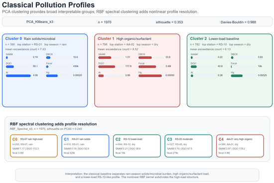
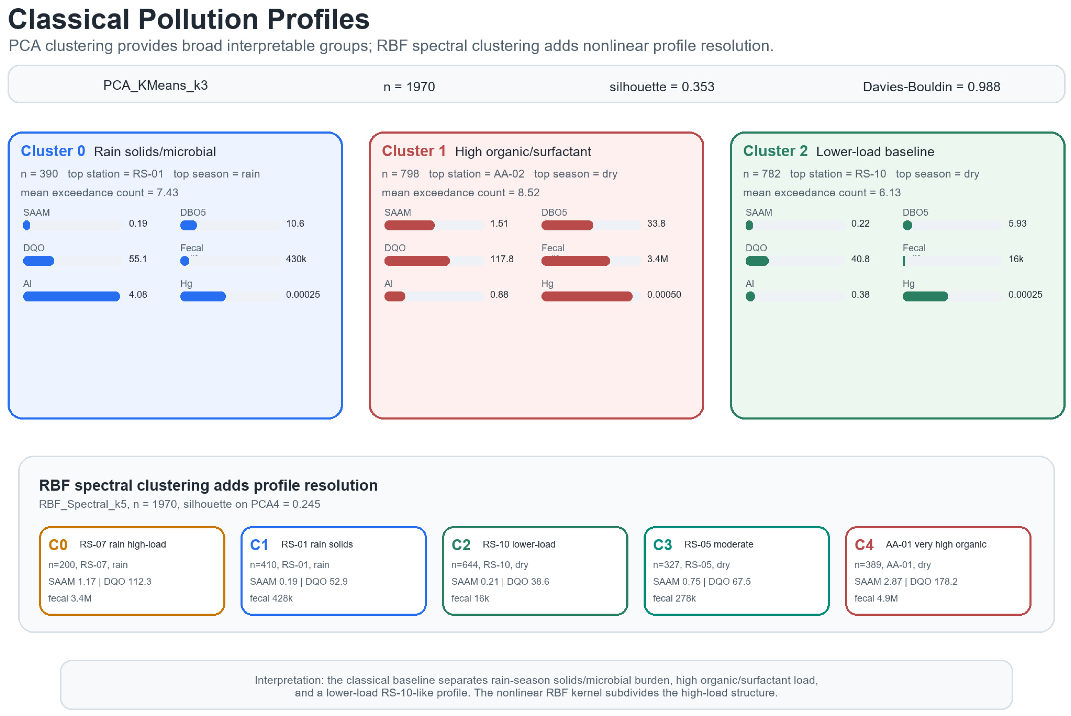
The most readable classical baseline is PCA_KMeans_k3. One cluster corresponds to a rain-season profile with higher solids, turbidity, and microbial burden. A second cluster represents the highest general pollution profile, with elevated SAAM, biochemical oxygen demand, chemical oxygen demand, ammoniacal nitrogen, conductivity, and coliforms. A third cluster has lower organic load, turbidity, coliforms, and exceedance counts, although it should not be interpreted as environmentally clean.

The RBF spectral clustering baseline adds finer resolution, separating a very high organic/SAAM profile, a high-load rain-season profile, a lower-load RS-10-like profile, a moderate conductivity/nutrient profile, and a rain/solids/microbial profile. These results suggest that nonlinear similarity measures can recover meaningful substructure beyond the broad PCA clusters.

Seasonal interpretation is particularly important because several profiles combine solids, turbidity, and microbial indicators in ways that are environmentally consistent with rainfall, runoff, and resuspension processes. The current data include calendar-derived season indicators, but not measured discharge or local rainfall totals. Therefore, rain-season cluster enrichment should be interpreted as hydrological context for profile interpretation rather than a direct flow-response model. Figure 6 summarizes the classical pollution-profile visualizations.

Figure 6. Classical pollution profiles from PCA_KMeans_k3 and RBF_Spectral_k5. PCA clustering separates broad rain-season solids/microbial, high organic/surfactant, and lower-load profiles, while the nonlinear RBF spectral baseline subdivides the high-load structure into more specific station-linked profiles.

3.7. Quantum-Kernel Pollution Profiles

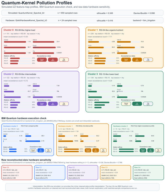
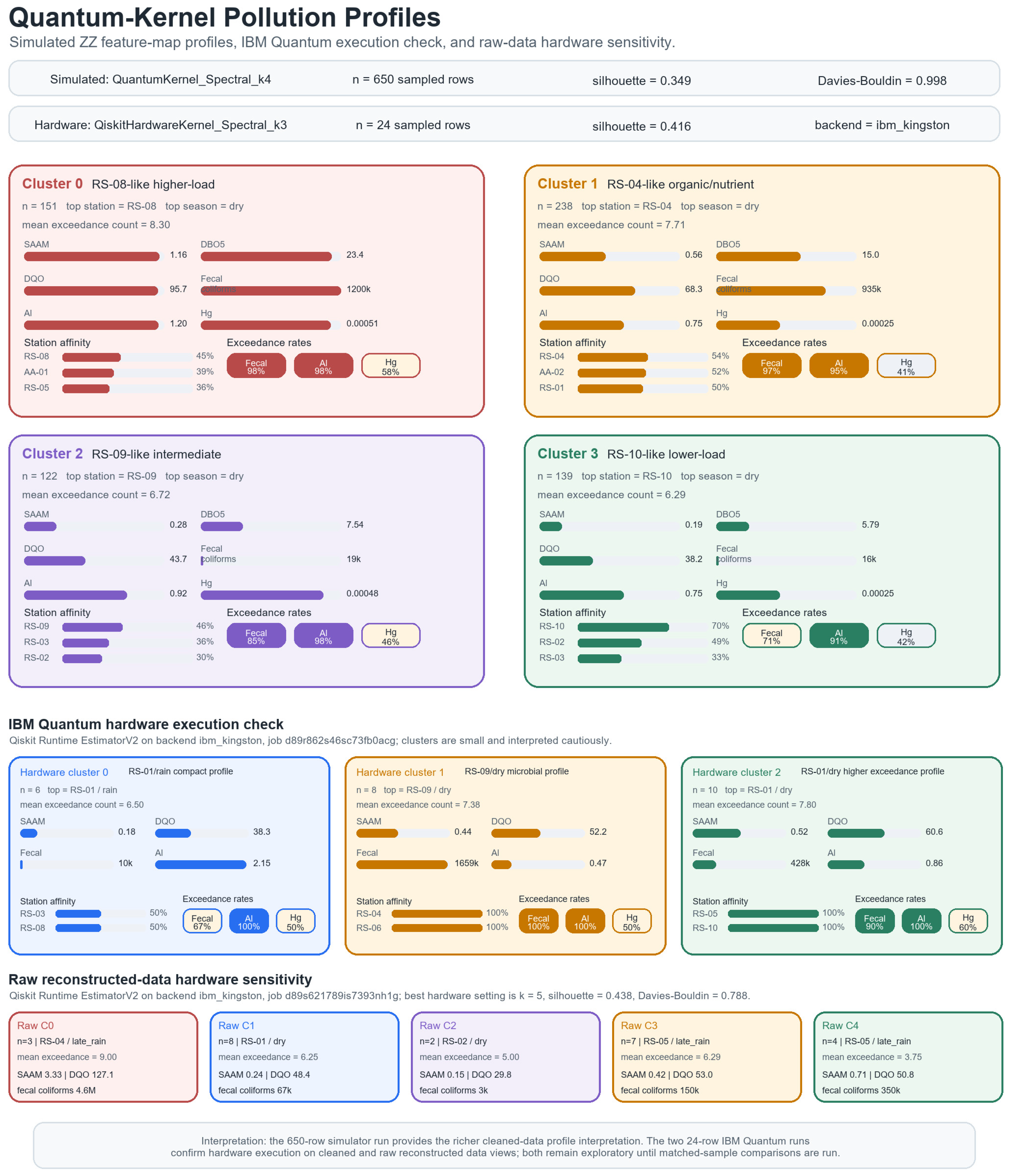
The most interpretable simulated quantum result remains QuantumKernel_Spectral_k4. The four profiles are provisionally read as: an RS-08-like higher-load profile with elevated SAAM, biochemical oxygen demand, chemical oxygen demand, coliforms, aluminum, and mercury exceedance; an RS-04-like moderate-high organic/nutrient profile; an RS-09-like intermediate profile with lower organic load but persistent exceedances; and an RS-10-like lower-load profile with the lowest chemical oxygen demand and SAAM medians among the quantum clusters.

The RS-08 association should be interpreted as a multivariate co-occurrence pattern rather than as direct source attribution. In the current analysis, the model indicates that samples associated with the RS-08-like profile jointly carry higher organic load, surfactant signal, fecal contamination, and selected metal exceedance indicators. Explaining why aluminum and mercury co-occur in that station-linked profile requires additional spatial evidence, including upstream land-use, industrial discharge, hydrological connectivity, and targeted geochemical records. Without those external data, the result is best framed as a hypothesis for environmental investigation rather than proof of a specific discharge source.

Geographically, this caution is important because the station codes do not map one-to-one onto individual discharge sources. RS-04 corresponds to Salto-Juanacatlán, AA-02 to El Muelle, and RS-08 to San Cristóbal de la Barranca in the monitoring-point table. The broader Santiago system receives mixed urban, industrial, agro-industrial, livestock, landfill, and agricultural inputs, with the El Salto-Juanacatlán and metropolitan-industrial corridor repeatedly identified as a critical pollution zone [15]. Therefore, RS-08-like or AA-02-linked clusters should be read as downstream or tributary-integrated chemical signatures until spatial source apportionment is added.

From an ecotoxicological perspective, the high-load signatures are plausible because the modeled variables correspond to common pressure pathways in the basin. Elevated biochemical and chemical oxygen demand, surfactants, ammoniacal nitrogen, conductivity, solids, turbidity, and fecal indicators are consistent with mixtures of municipal wastewater, industrial effluents, agro-industrial residues, livestock inputs, landfill leachate, and storm-driven resuspension or runoff. The Salto-Juanacatlán corridor is expected to concentrate urban-industrial and municipal pressures, whereas San Cristóbal de la Barranca should be interpreted more cautiously as a downstream integrator of upstream and tributary signals rather than as a single local source. This ecological reading supports the use of cluster signatures as screening hypotheses for targeted field validation, not as formal source attribution.

The same caution applies to emerging contaminants and emerging pollutants. The dataset used here contains conventional physicochemical, microbiological, surfactant, nutrient, solids, and selected metal variables; it does not include pharmaceuticals, pesticides, industrial transformation products, per- and poly-fluoroalkyl substances, microplastics, or high-resolution organic-screening markers. Consequently, the profiles can indicate pressure pathways that are compatible with emerging-contaminant concerns, but they cannot quantify those contaminants directly. Future monitoring could combine the present representation workflow with targeted or non-targeted chemical screening to test whether the learned profiles also stratify emerging-pollutant burdens.

The cleaned-data Qiskit hardware run provides a smaller but important execution check. On the 24-sample subset, QiskitHardwareKernel_Spectral_k3 achieved silhouette 0.416 and Davies-Bouldin 0.795, outperforming the k = 4 and k = 5 hardware-subset alternatives. Its three profiles are dominated by RS-01/rain, RS-09/dry, and RS-01/dry signatures, respectively, with mean exceedance counts between 6.5 and 7.8. The raw reconstructed hardware run produced a different optimum, with QiskitHardwareKernel_Spectral_k5 reaching silhouette 0.438 and Davies-Bouldin 0.788. These hardware profiles are reported as feasibility evidence and qualitative signatures.

This pattern suggests that the quantum feature map organizes observations along a station-linked pollution gradient. The matched 8-record run adds a useful control: when row membership is fixed, the cleaned and raw reconstructed kernels still prefer different cluster granularities, suggesting that the data-processing layer alters the encoded similarity geometry rather than merely changing which rows were sampled. Figure 7 summarizes the simulated and hardware quantum-kernel pollution-profile visualizations.

Figure 7. Quantum-kernel pollution profiles from the simulated QuantumKernel_Spectral_k4 cleaned-data run, the cleaned-data QiskitHardwareKernel_Spectral_k3 execution check, and the raw reconstructed-data QiskitHardwareKernel_Spectral_k5 sensitivity run. The simulator panel summarizes the richer 650-row station-linked gradient, while the IBM Quantum panels report 24-row hardware subsets executed on backend ibm_kingston under job IDs d89r862s46sc73fb0acg and d89s621789is7393nh1g.

4. Discussion

The initial findings support the value of representation learning for water-pollution profiling in complex river systems. Classical PCA produces broad and explainable clusters, while nonlinear kernels, including the simulated and hardware-executed quantum kernels, reveal additional station-linked structure. This finding is consistent with the broader water-quality machine learning literature, where model performance depends strongly on data volume, preprocessing, sensor design, and task definition [16,17]. The stability diagnostics reduce concern that the main n = 650 nonlinear results are artifacts of a single random seed; they also reinforce the central benchmark conclusion: the RBF kernel remains the strongest and most parsimonious nonlinear comparator under the present feature design.

The narrative hierarchy is therefore important. The classical geometry establishes what can already be learned from transparent and strong nonlinear baselines. The simulated quantum geometry tests an alternative phase-based representation of compact environmental coordinates. The hardware layer demonstrates that this representation can be executed through Qiskit Runtime on present IBM Quantum devices, but only at small sample sizes. The environmental interpretation layer then asks whether any of these geometries correspond to plausible station-linked pollution profiles. Reading the results in this order prevents the hardware subsets and raw-data sensitivity checks from overwhelming the main methodological message.

The new quantum-water-quality literature also helps position the present contribution. Al-karaki et al. report that QSVC was more practical than QNN for real-world Umgeni catchment classification, with QNN convergence problems under imbalanced field data [18]. Mauro et al. show that quantum preprocessing can reduce model parameters and improve turbidity prediction metrics in a remote-sensing setting [19]. These studies support a near-term view of QML as a representation or preprocessing strategy rather than as a guaranteed replacement for strong classical models. The Rio Santiago results follow that same pragmatic direction, but in an unsupervised clustering setting and with explicit clean/raw data-lineage controls.

Several limitations remain. First, the cleaned source data appear processed, and the raw reconstruction demonstrates that data-cleaning decisions materially change the clustering landscape. Second, the simulated and hardware quantum runs use smaller deterministic samples than some classical full-sample baselines, making matched controls essential. Third, the Qiskit hardware executions confirm feasibility on IBM Quantum infrastructure but are not large enough for final model selection. Fourth, UMAP, HDBSCAN, alternative Pauli feature maps, QSVC-style kernels, quanvolutional or hybrid preprocessing, quantum kernel PCA variants, and additional nonlinear classical baselines should be added before attributing any representational gain specifically to quantum encoding [18,19,21,22,23,24,25,26]. Fifth, station-level chemical interpretation requires external spatial and discharge evidence before cluster profiles can be linked to specific upstream sources.

In management terms, the method is best viewed as complementary to water-quality indices and regulatory exceedance analysis. WQIs summarize status in a compact score, while the clustering workflow preserves multivariate profile structure and can help prioritize which pollutant combinations, stations, or seasons deserve closer investigation [31]. This distinction is important for climate-sensitive water management: changing rainfall, runoff, and flow regimes can alter the timing and mixture of pollutant signals, so future versions should integrate discharge, precipitation, land-use, and source-inventory data before using clusters for operational management or climate-adaptation planning.

The immediate next step is therefore a controlled matched-sampling comparison in which PCA, RBF kernels, UMAP, HDBSCAN, simulated quantum kernels, and any feasible hardware kernels are run on the same deterministic samples for both cleaned and raw reconstructed data views. The n = 8 and n = 650 controls reported here demonstrate the workflow, but a fixed 24-record hardware-compatible subset should be used to compare all feasible methods under identical row membership, and a larger controlled subset, such as 200 or 650 records, should be used for simulator and classical methods. The resulting analyses should be interpreted with the same environmental summaries and tested for station and season stability.

5. Conclusions

This manuscript establishes a reproducible starting point for evaluating quantum machine learning as a tool for water-pollution profiling in the Rio Santiago basin. The quantum-kernel clusters are environmentally interpretable and appear to separate station-linked pollution states, while stability diagnostics show that the main simulated quantum geometry is not a seed artifact. The Qiskit runs confirm that the feature-map kernel can be executed on IBM Quantum hardware, with job IDs d89r862s46sc73fb0acg, d89s621789is7393nh1g, d89sqhlg7okc73ep3q70, and d8a7le8p0eas73dpgog0 archived in the project outputs. The raw reconstructed-data sensitivity analysis and matched controls show that data-cleaning choices affect the preferred clustering structure and kernel geometry. Modern nonlinear classical baselines, especially RBF and UMAP/HDBSCAN, remain strong competitors; the contribution is therefore a controlled and interpretable QML representation study rather than a claim of quantum advantage. The workflow may be transferable to lakes, groundwater, reservoirs, and other aquatic systems, but future applications should adapt the monitored variables and validation data to local hydrology, pollution sources, and management objectives.

References

- Fu, X.; Rol, M.A.; Bultink, C.C.; van Someren, J.; Khammassi, N.; Ashraf, I.; Vermeulen, R.F.L.; de Sterke, J.C.; Vlothuizen, W.J.; Schouten, R.N.; et al. An experimental microarchitecture for a superconducting quantum processor. In Proceedings of the 50th Annual IEEE/ACM International Symposium on Microarchitecture; Association for Computing Machinery: New York, NY, USA, 2017; Available online: https://dl.acm.org/doi/10.1145/3123939.3123952 (accessed on 20 June 2026).
- Barenco, A.; Bennett, C.; Cleve, R.; DiVincenzo, D.; Margolus, N.; Shor, P.; Sleator, T.; Smolin, J.; Weinfurter, H. Elementary gates for quantum computation. Phys. Rev. A 1995, 52, 3457–3467. [Google Scholar] [CrossRef] [Scilit] [PubMed]
- McKay, D.C.; Alexander, T.; Bello, L.; Biercuk, M.J.; Bishop, L.; Chen, J.; Chow, J.M.; Antonio, D.C.; Egger, D.; Filipp, S.; et al. Qiskit backend specifications for OpenQASM and OpenPulse experiments. arXiv 2018, arXiv:1809.03452v1. [Google Scholar]
- Peruzzo, A.; McClean, J.; Shadbolt, P.; Yung, M.-H.; Zhou, X.-Q.; Love, P.J.; Aspuru-Guzik, A.; O’Brien, J.L. A variational eigenvalue solver on a photonic quantum processor. Nat. Commun. 2014, 5, 4213. [Google Scholar] [CrossRef] [Scilit] [PubMed]
- Zúñiga-Grajeda, V.; Lomeli, J.A.; Villota-González, F.H.; García-García, C.A.; Sulbarán-Rangel, B. Estimation of Water Quality in Lakes and Rivers Using Remote Sensing and Artificial Intelligence: A Review of Image Processing and Validation Strategies. Limnol. Rev. 2026, 26, 19. [Google Scholar] [CrossRef] [Scilit]
- Recio, C.; Recio, R.; García, C.; Ezzahra, F.; Sandoval, J.; Espinoza, J.; Castañeda, A.; Ramírez, A.; Zurita, F.; Montoya, A.; et al. Investigación Interdisciplinaria en Ciencias Físicas, Ciencias de la Vida, Ingeniería e Informática en la Universidad de Guadalajara, 1st ed.; Editorial Universidad de Guadalajara: Guadalajara, Mexico, 2025. [Google Scholar] [CrossRef] [Scilit]
- Bollo Manent, M.; Hernandez Santana, J.; Mendez Linares, A. The state of the environment in Mexico. Open Geosci. 2014, 6, 219–228. [Google Scholar] [CrossRef] [Scilit]
- Dickey, D.A.; Fuller, W.A. Distribution of the estimators for autoregressive time series with a unit root. J. Am. Stat. Assoc. 1979, 74, 427–431. [Google Scholar] [CrossRef] [Scilit]
- González-Mariño, I.; Baz-Lomba, J.A.; Alygizakis, N.A.; Andrés-Costa, M.J.; Bade, R.; Bannwarth, A.; Barron, L.P.; Been, F.; Benaglia, L.; Berset, J.; et al. Spatio-temporal assessment of illicit drug use at large scale: Evidence from 7 years of international wastewater monitoring. Addiction 2020, 115, 109–120. [Google Scholar] [CrossRef] [Scilit] [PubMed]
- Hackathon HidroHack 2023 (fAIr LAC Jalisco). Agua.org.mx, 23 December 2022. Available online: https://agua.org.mx/convocatoria/hackathon-hidrohack-2023-fair-lac-jalisco/ (accessed on 20 June 2026).
- Howland, M.A. Methylene blue. In History of Modern Clinical Toxicology; Elsevier: Amsterdam, The Netherlands, 2022; pp. 231–241. [Google Scholar] [CrossRef] [Scilit]
- NOM-127-SSA1-2021; Agua para Uso y Consumo Humano. Límites Permisibles de la Calidad del agua. Comité Consultivo Nacional de Normalización de Regulación y Fomento Sanitario: Ciudad de México, México, 2021.
- McInnes, L.; Healy, J.; Melville, J. UMAP: Uniform Manifold Approximation and Projection for Dimension Reduction. arXiv 2018, arXiv:1802.03426. [Google Scholar]
- McInnes, L.; Healy, J.; Astels, S. hdbscan: Hierarchical density based clustering. J. Open Source Softw. 2017, 2, 205. [Google Scholar] [CrossRef] [Scilit]
- Valdovinos-Flores, C. Industrialization and its environmental impact on health and pollution in the Santiago River Basin of Mexico. Int. J. Environ. Sci. Technol. 2025, 22, 16247–16260. [Google Scholar] [CrossRef] [Scilit]
- Dharma, V.L.; Nurtanio, N.K.; Nugroho, F.S.; Anggreainy, M.S.; Kurniawan, A. A Review on Machine Learning Methods for Water Quality Prediction. In Proceedings of the 2023 4th International Conference on Artificial Intelligence and Data Sciences (AiDAS); IEEE: New York, NY, USA, 2023. [Google Scholar] [CrossRef] [Scilit]
- Rahu, M.A.; Chandio, A.F.; Aurangzeb, K.; Karim, S.; Alhussein, M.A.; Anwar, M.S. Toward Design of Internet of Things and Machine Learning-Enabled Frameworks for Analysis and Prediction of Water Quality. IEEE Access 2023, 11, 101055–101086. [Google Scholar] [CrossRef] [Scilit]
- Al-karaki, J.; Khan, M.A.-Z.; Gawanmeh, A.; Omar, M. Predicting water quality using quantum machine learning: The case of the Umgeni catchment (U20A) study region. Ain Shams Eng. J. 2026, 17, 103925. [Google Scholar] [CrossRef] [Scilit]
- Mauro, F.; Razzano, F.; Di Stasio, P.; Sebastianelli, A.; Meoni, G.; Schirinzi, G.; Gamba, P.; Ullo, S. Quantum-Enhanced Water Quality Monitoring: Exploiting Phi-Sat-2 Data with Quanvolution. IEEE Geosci. Remote Sens. Lett. 2025, 22, 1502905. [Google Scholar] [CrossRef] [Scilit]
- Biamonte, J.; Wittek, P.; Pancotti, N.; Rebentrost, P.; Wiebe, N.; Lloyd, S. Quantum machine learning. Nature 2017, 549, 195–202. [Google Scholar] [CrossRef] [Scilit] [PubMed]
- Havlicek, V.; Corcoles, A.D.; Temme, K.; Harrow, A.W.; Kandala, A.; Chow, J.M.; Gambetta, J.M. Supervised learning with quantum-enhanced feature spaces. Nature 2019, 567, 209–212. [Google Scholar] [CrossRef] [Scilit] [PubMed]
- Schuld, M. Supervised quantum machine learning models are kernel methods. arXiv 2021, arXiv:2101.11020. [Google Scholar]
- Huang, H.-Y.; Broughton, M.; Mohseni, M.; Babbush, R.; Boixo, S.; Neven, H.; McClean, J.R. Power of data in quantum machine learning. Nat. Commun. 2021, 12, 2631. [Google Scholar] [CrossRef] [Scilit] [PubMed]
- Cerezo, M.; Arrasmith, A.; Babbush, R.; Benjamin, S.C.; Endo, S.; Fujii, K.; McClean, J.R.; Mitarai, K.; Yuan, X.; Cincio, L.; et al. Variational quantum algorithms. Nat. Rev. Phys. 2021, 3, 625–644. [Google Scholar] [CrossRef] [Scilit]
- Bharti, K.; Cervera-Lierta, A.; Kyaw, T.H.; Haug, T.; Alperin-Lea, S.; Anand, A.; Degroote, M.; Heimonen, H.; Kottmann, J.S.; Menke, T.; et al. Noisy intermediate-scale quantum algorithms. Rev. Mod. Phys. 2022, 94, 015004. [Google Scholar] [CrossRef] [Scilit]
- Wang, Y. Near-optimal quantum kernel principal component analysis. Quantum Sci. Technol. 2025, 10, 015034. [Google Scholar] [CrossRef] [Scilit]
- González-Díaz, R.L.; de Anda, J.; Shear, H.; Padilla-Tovar, L.E.; Lugo-Melchor, O.Y.; Olvera-Vargas, L.A. Assessment of Heavy Metals in Surface Waters of the Santiago-Guadalajara River Basin, Mexico. Hydrology 2025, 12, 37. [Google Scholar] [CrossRef] [Scilit]
- Alvarez-Alonso, R.; Robledo Ardila, P.A.; Deudero, S.; Melo-Aguilar, C.A.; Alomar, C.; Micheo, F.; Duran, J.J.; Pérez, S.; Arcega Cabrera, F.; Martinez Pérez, S. Multivariate assessment of groundwater contamination levels associated with saline intrusion processes in Mediterranean coastal aquifers. J. Contam. Hydrol. 2026, 278, 104877. [Google Scholar] [CrossRef] [Scilit] [PubMed]
- Anand, V.; Oinam, B.; Wieprecht, S. Machine learning approach for water quality predictions based on multispectral satellite imageries. Ecol. Inform. 2024, 84, 102868. [Google Scholar] [CrossRef] [Scilit]
- Georgescu, L.P.; Balsalobre-Lorente, D.; Zlati, M.L.; Fortea, C.; Antohi, V.-M.; Barbuta-Misu, N. Cluster Analysis of the Transition to Climate Neutrality in the European Union. Sustain. Dev. 2025, 33, 1498–1519. [Google Scholar] [CrossRef] [Scilit]
- Iticescu, C.; Murariu, G.; Georgescu, L.P.; Burada, A.; Topa, C.M. Seasonal Variation of the Physico-chemical Parameters and Water Quality Index (WQI) of Danube Water in the Transborder Lower Danube Area. Rev. Chim. 2016, 67, 1843–1849. [Google Scholar]
Disclaimer/Publisher’s Note: The statements, opinions and data contained in all publications are solely those of the individual author(s) and contributor(s) and not of MDPI and/or the editor(s). MDPI and/or the editor(s) disclaim responsibility for any injury to people or property resulting from any ideas, methods, instructions or products referred to in the content. |
© 2026 by the authors. Licensee MDPI, Basel, Switzerland. This article is an open access article distributed under the terms and conditions of the Creative Commons Attribution (CC BY) license.