Energy Consumption Prediction for an Electric Vehicle Using Machine Learning: A Comparative Study of Regression, Ensemble, and LSTM-Based Models

Abstract

Accurate energy consumption prediction is fundamental for enhancing range estimation and trip planning in battery electric vehicles (BEVs) under real-world conditions. This study develops a route-level benchmark utilizing 1 Hz data acquired via ECU/OBD-II interfaces (CAN 500 kbps) across ten diverse real-world driving routes. The input feature set comprises vehicle speed, longitudinal acceleration, estimated motor torque, road altitude, and accelerator pedal position. Ground truth energy consumption was derived from battery voltage and current, integrated via the trapezoidal rule. We performed a comparative analysis between five memoryless regressors (FNN, SVR, GPR, QRNN, and Bagged Trees) and three sequence models (LSTM, GRU, and BiLSTM) trained on 20-second temporal windows. The results indicate that the GRU model achieved the highest overall performance (mean RMSE = 0.1142 kWh, R² = 0.9545 and MAE = 0.072 kWh), while Bagged Trees emerged as the most robust static model (mean RMSE = 0.1587 kWh). Temporal models outperformed static ones on routes with high dynamic variability, whereas Bagged Trees excelled in five specific scenarios. These findings provide a controlled within-route benchmark for time-resolved cumulative energy estimation and highlight the need for chronological and cross-route validation before drawing deployment-oriented generalization claims.

1. Introduction

Battery electric vehicles (BEVs) require accurate energy consumption forecasting to ensure reliable range estimation, optimize route planning, and support real-time energy management strategies. Predictive models capable of estimating cumulative energy demand along a route contribute directly to reducing range uncertainty and improving operational efficiency [1,2]. Unlike internal battery state reconstruction, energy consumption prediction focuses on the vehicle-level energy demand driven by real-world operating conditions.

The novelty of this study does not primarily lie in proposing fundamentally new machine learning architectures but in systematically formulating and comparatively evaluating second-by-second cumulative energy prediction as a route-level forecasting problem for battery electric vehicles. This framing is particularly relevant from an application standpoint, as high-temporal-resolution cumulative energy estimates can support real-time energy management, eco-driving assistance, and range-aware onboard decision-making.

Accurately forecasting BEV energy consumption remains challenging because energy demand evolves under nonlinear and time-varying operating conditions [1,3]. Although physics-based models offer physical interpretability, they typically require detailed parameter identification and high-fidelity sensing, which may not always be available in real-world deployments. These limitations have motivated the increasing adoption of data-driven machine learning (ML) approaches capable of learning complex nonlinear relationships directly from operational driving data [2].

The recent literature spans classical regression, kernel-based learning, tree ensembles, advanced boosting, recurrent neural networks, and hybrid physical–machine learning approaches. Classical regression methods such as Ridge and Lasso provide interpretable baselines but often struggle to capture complex nonlinear interactions [4,5]. Kernel-based approaches such as Support Vector Regression (SVR) improve nonlinear modeling performance but remain sensitive to hyperparameter selection [6,7]. Tree-based ensemble methods and advanced boosting strategies, including XGBoost, LightGBM, and CatBoost, have shown strong performance in EV energy consumption and range-related tasks, especially under real-world datasets [8,9,10,11,12]. Recurrent neural networks such as LSTM and GRU are particularly suitable for temporally structured prediction problems, while hybrid sequential architectures have also reported strong performance in dynamic modeling tasks [13,14,15,16,17]. Methodologically related areas, including battery state estimation, physics-informed learning, and reinforcement learning, provide useful insights into nonlinear, temporal, and adaptive modeling, although they are not directly equivalent to route-level cumulative energy forecasting [18,19,20,21,22,23,24]. Recent studies have also extended the field toward interpretable energy modeling and infrastructure-influenced energy analysis [25,26]; however, second-by-second cumulative forecasting in BEVs remains insufficiently addressed.

Despite recent progress, several limitations in the literature motivate the present study. First, many prior works focus on trip-level total energy prediction, charging demand estimation, or aggregated consumption metrics rather than second-by-second cumulative route-level forecasting [9,11,27,28]. Consequently, the prediction target addressed in much of the literature differs substantially from the one considered here. In the present work, cumulative energy must be estimated continuously along the route at high temporal resolution, making the problem inherently sequential and path-dependent rather than purely static or end-of-trip oriented.

Second, previously reported results should be interpreted with caution because comparisons across model families are often conducted under heterogeneous experimental conditions. Differences in preprocessing pipelines, feature availability, dataset composition, temporal granularity, and validation design make it difficult to determine whether the reported performance gains arise from the learning paradigm itself or from the surrounding experimental setup [9,11,29]. Therefore, high reported values of R² or low prediction errors do not necessarily imply direct methodological superiority when studies address distinct targets such as trip-level consumption, range prediction, or instantaneous power estimation. This lack of methodological homogeneity also limits fair comparison across memoryless regressors, ensemble methods, and recurrent architectures.

Third, although several studies report excellent predictive performance, the trade-off between model complexity, temporal modeling capability, and practical deployability in embedded automotive systems remains insufficiently characterized [29,30,31]. This issue is particularly relevant for real-time onboard applications, where computational efficiency, causal inference, and robustness under dynamic driving conditions are as important as predictive accuracy itself. As a result, the literature still lacks a controlled assessment of which model families are most appropriate when cumulative energy must be predicted continuously under realistic route conditions.

These limitations motivate the need for a controlled and analytically structured benchmark. In this work, second-by-second cumulative route-level forecasting is treated as a distinct and practically meaningful task rather than as a direct extension of trip-level or aggregated energy estimation. From this perspective, the contributions of the present study lie in the following: (i) formulating cumulative energy prediction as a many-to-one sequence regression problem aligned with the temporal integration of power demand; (ii) establishing a route-level benchmark based on 1 Hz real-world telemetry and homogeneous preprocessing, normalization, and evaluation conditions; (iii) providing controlled empirical evidence on how different model classes behave under this formulation, particularly under varying route dynamics.

Table 1 summarizes representative recent studies on EV energy consumption prediction, integrating predictive performance with deployability considerations [9,11,29]. This comparison is not intended as a strict quantitative ranking across prior works, since the reviewed studies differ in target definition, temporal resolution, dataset composition, and validation protocol. Instead, it is used to position representative model families under heterogeneous real-world and operational settings and to clarify the specific gap addressed by this study. This perspective is also consistent with recent reviews showing that a substantial portion of the literature remains centered on remaining driving range prediction and related energy-oriented tasks rather than on high-resolution cumulative route-level forecasting [32].

Within this context, transformer-based approaches such as TabTransformer report very high predictive accuracy [29], but their computational burden may reduce their suitability for embedded real-time deployment. In contrast, optimized boosting frameworks such as Bayesian-tuned LightGBM and XGBoost offer a more favorable balance between predictive performance and computational efficiency [9,11,30]. KNN-based hybrid approaches have also shown competitive performance in BEV charging datasets when combined with appropriate hyperparameter optimization, further illustrating the importance of model tuning in energy-related prediction tasks [9,33]. Regression-based approaches have likewise been applied to domain-specific electric vehicle drive cycles, showing that relatively simple models may remain effective when the operating scenario is constrained and well characterized [34]. Hybrid physical–machine learning models further improve robustness under real-world driving variability, particularly in route-level and mid-term estimation scenarios [28,31]. Sequential deep learning models are also especially relevant for high-resolution prediction tasks. For example, Chen et al. [35] showed, using 1 Hz real-world electric bus data, that recurrent models outperform feedforward alternatives in temporally structured energy estimation. Although that study addressed instantaneous power-related dynamics rather than cumulative route-level forecasting, it supports the broader view that temporally structured models are better aligned with high-resolution sequential prediction tasks. Ensemble-based AutoML approaches have likewise been explored for micro-trip energy prediction in electric two-wheelers, highlighting the sensitivity of model performance to route segmentation and variability effects [27].

Table 1. Comparative Framework of Machine Learning Models for BEV Energy Consumption Prediction.

Method/Approach	Category	Dataset Type	Reported Performance	Relevance to Energy Consumption Study	Ref.
TabTransformer	Deep Learning (Transformer Tabular)	Volkswagen e-Golf (3345 samples)	R2 = 0.9812	State-of-the-art short-term energy consumption prediction; highest accuracy benchmark	[29]
LightGBM (Bayesian Optimized)	Advanced Boosting	Volkswagen e-Golf (3345 samples)	R2 = 0.9808	Optimal trade-off between predictive accuracy and computational efficiency for real-time energy estimation	[9,29]
ANN (Partition-Based)	Deep Learning (Feedforward NN)	Real-world electric bus (2600 h, 1 Hz)	MAPE ≈ 5%	Microscopic instantaneous power modeling with charging/discharging partition strategy; validated using 10-fold cross-validation	[35]
LSTM (Sequential Modeling)	Deep Learning (Recurrent NN)	Real-world electric bus (2600 h, 1 Hz)	MAPE ≈ 3%	High-resolution temporal energy modeling; captures sequential dependencies and improves cumulative prediction accuracy	[35]
Cooperative KNN-RF	KNN-based Hybrid ML	Real-world electric bus big data	MAE improved by 9.47–51.14%, computation time reduced by up to 97.14%	KNN-based hybrid modeling can improve EV energy prediction with high computational efficiency	[33]
Polynomial Regression	Regression Model	Nissan Leaf urban driving cycles	R2 = 0.9652	Embedded-ready consumption estimation under domain-specific driving cycles	[34]
XGBoost	Gradient Boosting	Tesla Model S real-world dataset	R2 = 0.9186, RMSE = 9.49 kWh	Robust nonlinear modeling for total energy consumption forecasting	[11,30]
Support Vector Regression (SVR)	Kernel-Based ML	Tesla Model S real-world dataset	R2 = 0.8848, RMSE = 10.71 kWh	Nonlinear baseline for TEC modeling; higher computational burden	[11]
Multiple Linear Regression (MLR)	Linear ML	Tesla Model S real-world dataset	R2 = 0.8342, RMSE = 12.93 kWh	Classical regression benchmark for energy consumption modeling	[11,32]
Stacked Ensemble (AutoML)	Ensemble ML	Electric Two-Wheelers	R2 ≈ 0.75–0.78	Ensemble-based micro-trip energy prediction; highlights variability effects	[27]
HMM + ECM Hybrid	Hybrid Physical + ML	Real-world personalized driving dataset	Relative error < 10%	Physics-informed consumption and range estimation under real traffic variability	[31]
Correlation-Based ML	Statistical + ML	Connected BEV operational dataset	R2 = 0.7685	Multi-factor route-level energy modeling baseline	[28]

Table 1. Comparative Framework of Machine Learning Models for BEV Energy Consumption Prediction.

Method/Approach	Category	Dataset Type	Reported Performance	Relevance to Energy Consumption Study	Ref.
TabTransformer	Deep Learning (Transformer Tabular)	Volkswagen e-Golf (3345 samples)	R2 = 0.9812	State-of-the-art short-term energy consumption prediction; highest accuracy benchmark	[29]
LightGBM (Bayesian Optimized)	Advanced Boosting	Volkswagen e-Golf (3345 samples)	R2 = 0.9808	Optimal trade-off between predictive accuracy and computational efficiency for real-time energy estimation	[9,29]
ANN (Partition-Based)	Deep Learning (Feedforward NN)	Real-world electric bus (2600 h, 1 Hz)	MAPE ≈ 5%	Microscopic instantaneous power modeling with charging/discharging partition strategy; validated using 10-fold cross-validation	[35]
LSTM (Sequential Modeling)	Deep Learning (Recurrent NN)	Real-world electric bus (2600 h, 1 Hz)	MAPE ≈ 3%	High-resolution temporal energy modeling; captures sequential dependencies and improves cumulative prediction accuracy	[35]
Cooperative KNN-RF	KNN-based Hybrid ML	Real-world electric bus big data	MAE improved by 9.47–51.14%, computation time reduced by up to 97.14%	KNN-based hybrid modeling can improve EV energy prediction with high computational efficiency	[33]
Polynomial Regression	Regression Model	Nissan Leaf urban driving cycles	R2 = 0.9652	Embedded-ready consumption estimation under domain-specific driving cycles	[34]
XGBoost	Gradient Boosting	Tesla Model S real-world dataset	R2 = 0.9186, RMSE = 9.49 kWh	Robust nonlinear modeling for total energy consumption forecasting	[11,30]
Support Vector Regression (SVR)	Kernel-Based ML	Tesla Model S real-world dataset	R2 = 0.8848, RMSE = 10.71 kWh	Nonlinear baseline for TEC modeling; higher computational burden	[11]
Multiple Linear Regression (MLR)	Linear ML	Tesla Model S real-world dataset	R2 = 0.8342, RMSE = 12.93 kWh	Classical regression benchmark for energy consumption modeling	[11,32]
Stacked Ensemble (AutoML)	Ensemble ML	Electric Two-Wheelers	R2 ≈ 0.75–0.78	Ensemble-based micro-trip energy prediction; highlights variability effects	[27]
HMM + ECM Hybrid	Hybrid Physical + ML	Real-world personalized driving dataset	Relative error < 10%	Physics-informed consumption and range estimation under real traffic variability	[31]
Correlation-Based ML	Statistical + ML	Connected BEV operational dataset	R2 = 0.7685	Multi-factor route-level energy modeling baseline	[28]

Overall, the reviewed literature indicates that model superiority in BEV energy prediction is highly task-dependent and should be interpreted cautiously. Within this context, the present study is positioned as a controlled route-level benchmark for second-by-second cumulative energy prediction in battery electric vehicles using real-world data and uniform evaluation conditions.

To address this gap, the study compares eight machine-learning models for second-by-second cumulative energy prediction using 1 Hz telemetry collected from ten real-world routes of a Kia Soul EV. The benchmark includes five memoryless regression approaches—Feedforward Neural Network (FNN), Support Vector Regression (SVR), Gaussian Process Regression (GPR), Quantile Regression Neural Network (QRNN), and Bagged Trees—and three sequence-aware recurrent architectures—LSTM, GRU, and BiLSTM. By evaluating all models under a common route-level framework, the study enables a fairer comparison in which performance differences can be attributed more directly to modeling behavior than to inconsistencies in preprocessing or evaluation design.

Main Contributions

This study contributes to battery electric vehicle (BEV) energy modeling in three main ways. The principal contributions are as follows:

• First, it formulates second-by-second cumulative energy consumption prediction as a many-to-one sequence regression problem, explicitly aligning the learning objective with the physical integration of power demand over time.
• Second, it establishes a controlled route-level benchmark based on 1 Hz real-world telemetry collected over ten driving routes, enabling a fair comparison of eight modeling paradigms under identical preprocessing, normalization, and partitioning conditions.
• Third, it provides controlled empirical evidence that recurrent architectures, particularly the GRU model adopted in this study, are advantageous under within-route benchmarking conditions for dynamic cumulative energy estimation, while also showing that memoryless models, especially Bagged Trees, can remain competitive under smoother route conditions.

The remainder of this paper is organized as follows: Section 2 describes the data acquisition process, preprocessing strategy, and evaluated models. Section 3 presents the comparative experimental results. Section 4 discusses the main findings, practical implications, and limitations. Finally, Section 5 concludes the paper and outlines directions for future work.

2. Materials and Methods

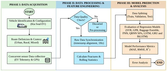
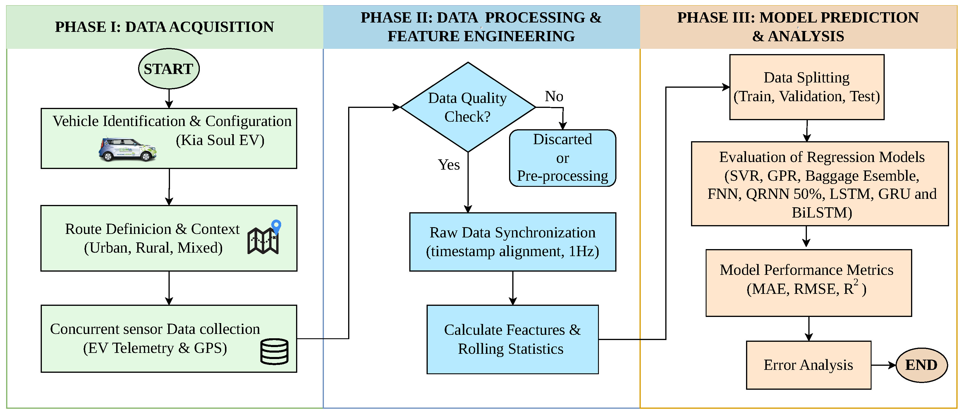
Figure 1 summarizes the proposed three-phase framework, which comprises data acquisition, data preprocessing, and model training and evaluation. In Phase I, synchronized telemetry data sampled at 1 Hz were collected from a Kia Soul BEV under diverse real-world driving conditions, including urban, rural, and mixed routes. In Phase II, the raw signals were validated, temporally aligned, and transformed into the predictor–target structure used for supervised learning. In Phase III, multiple regression paradigms were trained and comparatively evaluated, including memoryless models (FNN, SVR, GPR, QRNN, and Bagged Trees) and sequence-aware recurrent models (LSTM, GRU, and BiLSTM). Model performance was assessed using RMSE, MAE, and R².

Figure 1. Three-phase methodology adopted in this study, including route-level data acquisition, preprocessing and benchmark construction, and comparative model training and evaluation.

2.1. Phase I: Data Acquisition

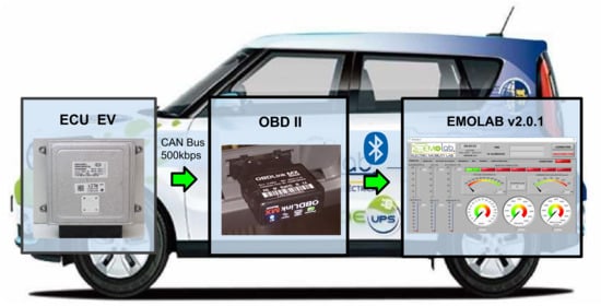
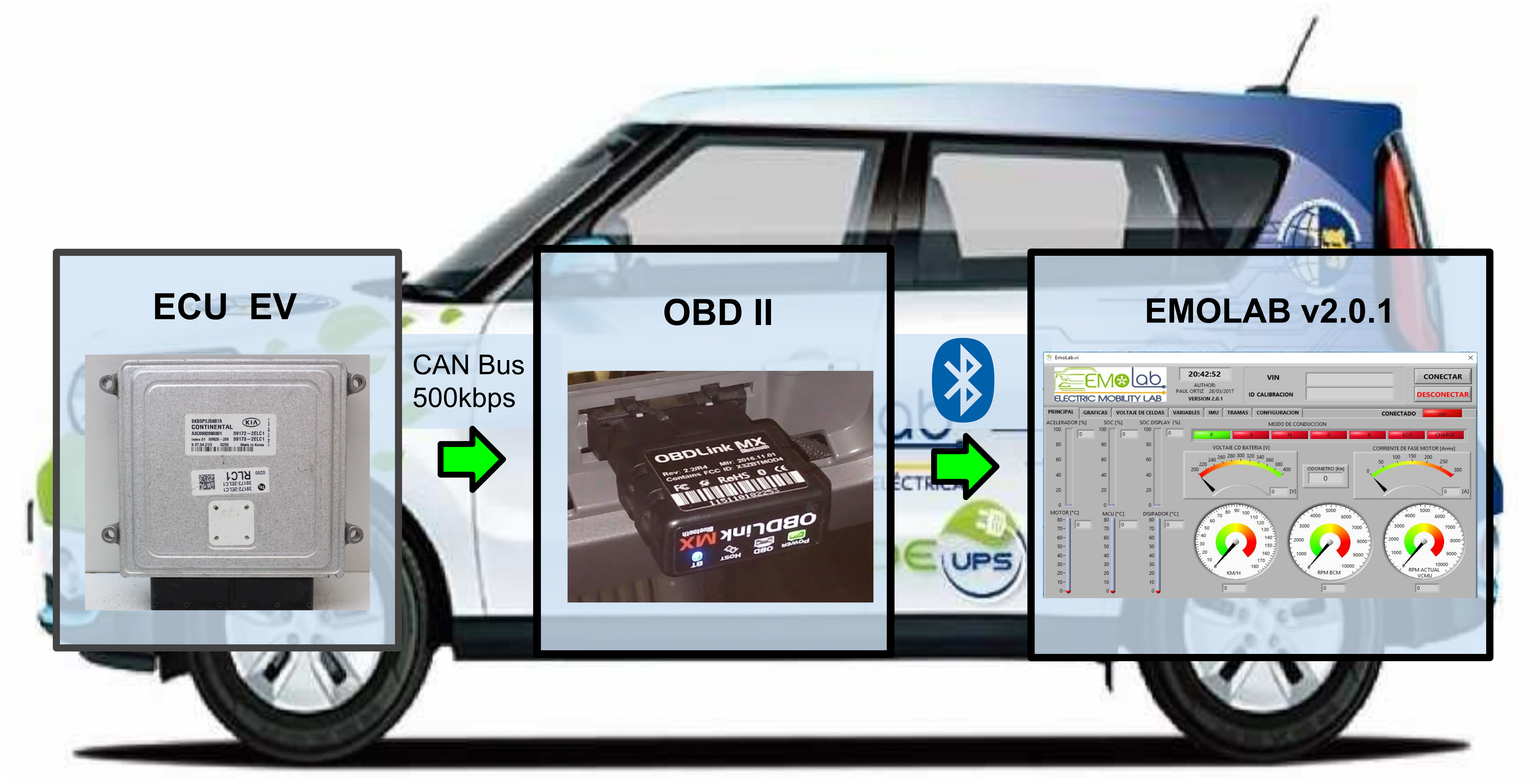
The dataset used in this study comprises operational records acquired from the Electronic Control Unit (ECU) of a battery electric vehicle (BEV) driven along ten distinct real-world routes. The data acquisition architecture is illustrated in Figure 2. Vehicle operational parameters were accessed through the OBD-II interface using Controller Area Network (CAN) communication at a baud rate of 500 kbps. The OBD-II module transmitted the recorded signals to the EMOLAB v2.0.1 data-logging software via Bluetooth, with a uniform sampling frequency of 1 Hz.

Figure 2. Route-level telemetry acquisition architecture used in this study, showing ECU/OBD-II access, CAN communication at 500 kbps, Bluetooth transmission, and data logging in EMOLAB v2.0.1.

The experimental campaigns were conducted in Cuenca, Ecuador, at an average altitude of approximately 2500 m above sea level. This high-altitude operating environment is relevant because reduced air density and local topographical variability may affect vehicle energy consumption dynamics.

Three derived variables were computed before model fitting:

• Acceleration (a): longitudinal acceleration in m/s², computed as the first difference of speed after conversion to m/s.
• Instantaneous electric power (P): computed at each time step from battery voltage and current, and expressed in kW.
• Cumulative energy (E): the target variable, obtained by trapezoidal integration of power over time and converted to kWh. By definition, $E\left(0\right)=0$ and the signal increases monotonically during the trip.

For modeling purposes, the input feature vector at each time step was defined as

$$\mathbf{x}\left(t\right)=\left[v\left(t\right),a\left(t\right),{\tau }_{\mathrm{est}}\left(t\right),h\left(t\right),p\left(t\right)\right]\in {\mathbb{R}}^5,$$

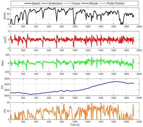
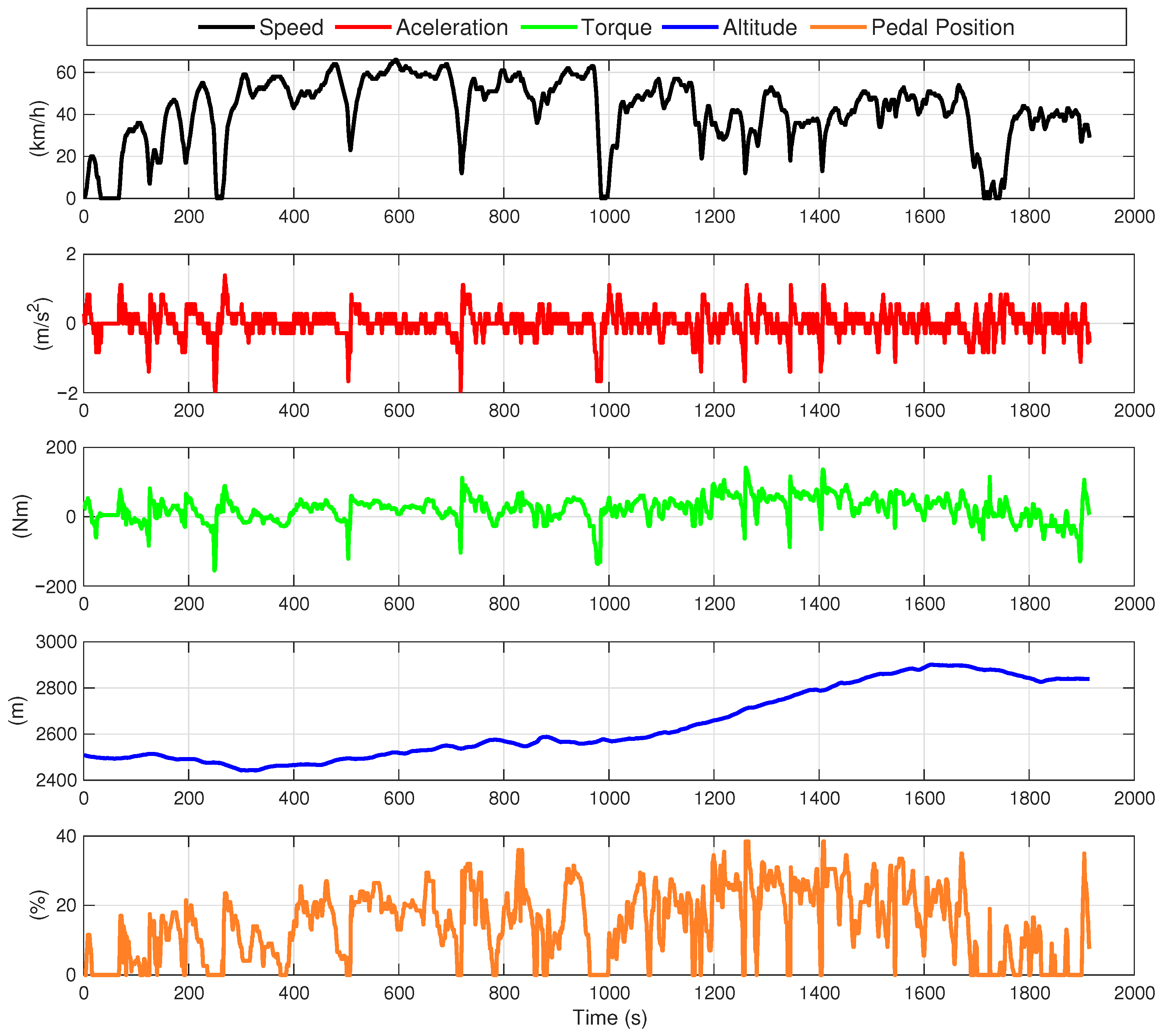
where $v\left(t\right)$ is vehicle speed, $a\left(t\right)$ is longitudinal acceleration, ${\tau }_{\mathrm{est}}\left(t\right)$ is estimated motor torque, $h\left(t\right)$ is road altitude, and $p\left(t\right)$ is accelerator pedal position. Figure 3 shows these variables for Route 1.

Figure 3. Measured input variables for Route 1: speed, acceleration, altitude, and pedal position.

2.2. Phase II: Data Processing and Benchmark Design

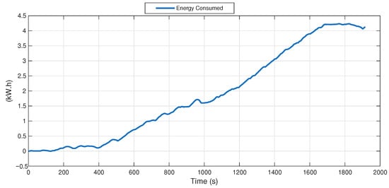
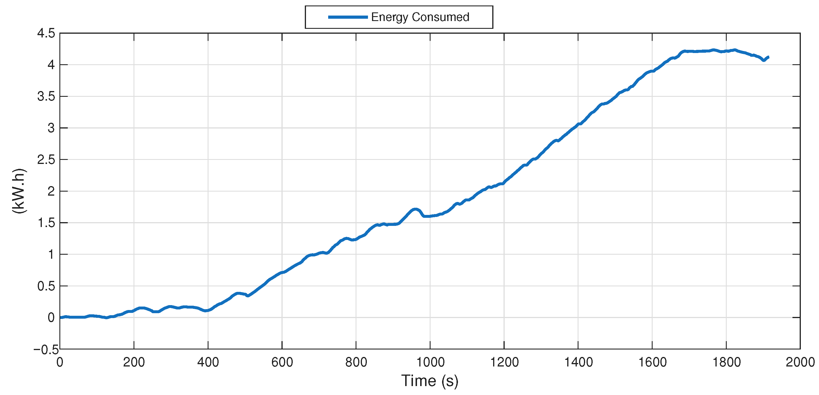
The five input variables at time step t were used to predict the cumulative energy consumption $E\left(t\right)$. Since $E\left(t\right)$ is the temporal integral of electrical power, its value depends on the history of prior vehicle operation and cannot, in general, be uniquely determined from a single instantaneous observation alone. This motivates the use of sequence-aware models capable of exploiting temporal context. Figure 4 illustrates the cumulative energy profile for Route 1.

Figure 4. Measured cumulative energy profile for Route 1, used to illustrate the path-dependent nature of the prediction target and motivate the use of sequence-aware models.

It is important to emphasize that direct electrical measurements such as battery current, voltage, and instantaneous power were not included as predictors. Therefore, the models were required to infer cumulative energy exclusively from vehicle dynamics, road profile, and driver-demand variables, making temporal modeling especially relevant.

Each route dataset was partitioned into a training set (70% of the samples) and a testing set (30%) using route-wise random holdout splitting. This protocol was adopted to establish a controlled within-route comparative benchmark under identical preprocessing, normalization, and model-training conditions across all evaluated methods. We emphasize that this design does not constitute strict chronological forecasting, since samples from later portions of the route may be represented in the training subset. Therefore, the reported results should be interpreted as comparative within-route regression performance rather than as evidence of deployment-oriented temporal generalization.

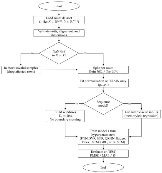
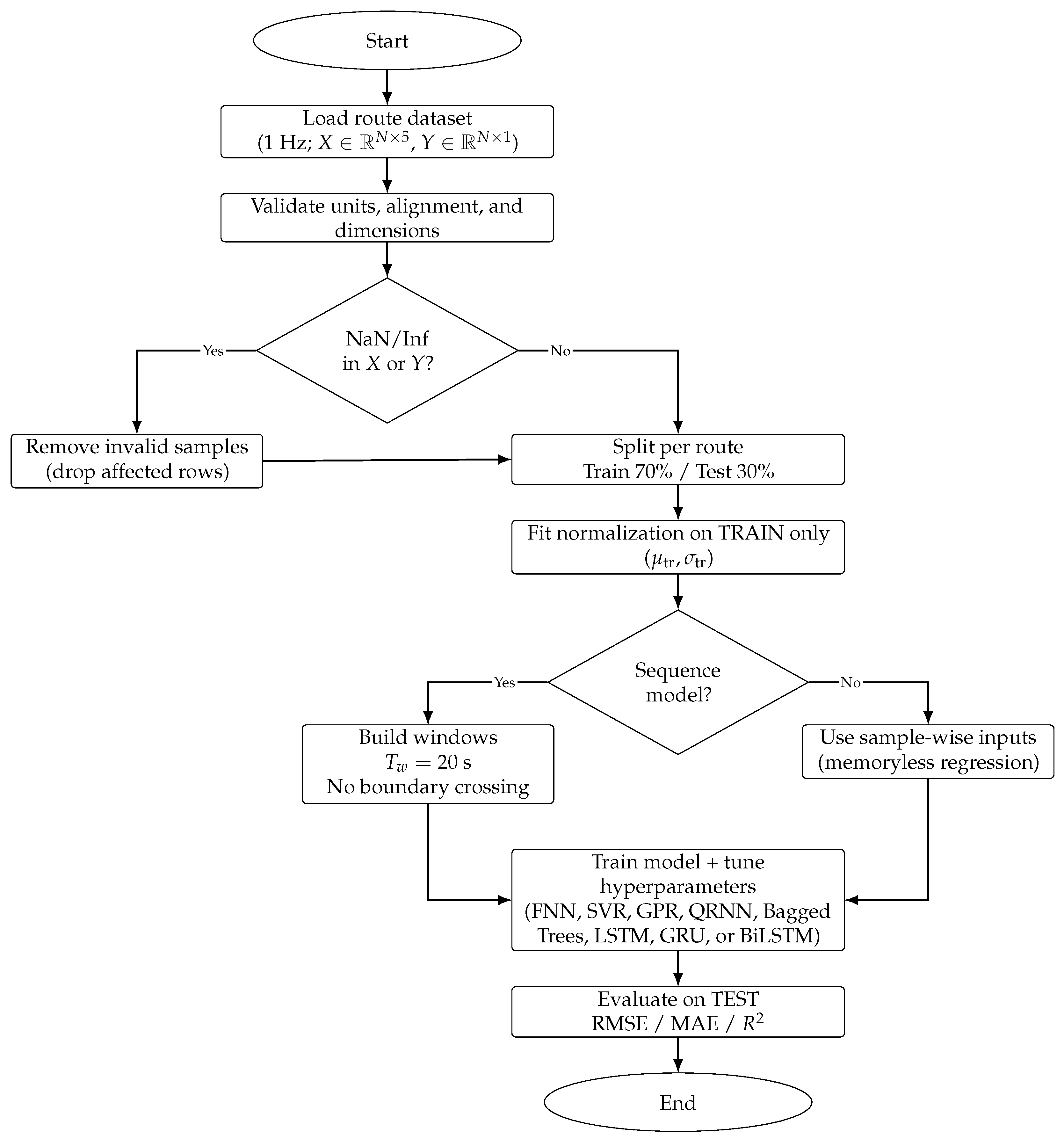
Figure 5 summarizes the preprocessing and evaluation workflow. Any invalid or non-finite observations (NaN/Inf) were removed before model fitting. Feature normalization parameters were estimated exclusively from the training subset and then applied unchanged to the testing subset. For sequence-based models, temporal causality was preserved within each training sample by constructing sliding windows only from past observations and by preventing boundary crossing between partitions.

Figure 5. Preprocessing workflow and evaluation pipeline for BEV route datasets.

2.3. Phase III: Regression Models Evaluated

For reproducibility, the corresponding MATLAB implementation details for all models are provided in Appendix A. The main text focuses on methodological principles, compact formulations, and relevant hyperparameter choices. A broad spectrum of regression models, from classical nonlinear regressors to recurrent neural networks, was implemented using MATLAB regression and Deep Learning toolboxes. To improve clarity and notation consistency, the main symbols used throughout this section are defined once below.

• Notation.

Let $\mathbf{x}\left(t\right)\in {\mathbb{R}}^5$ denote the input vector at time step t, and let $y\left(t\right)=E\left(t\right)\in \mathbb{R}$ denote the cumulative energy consumed up to time t. For sequence-based models, an input window of length $T_w$ is defined as

$${\mathbf{X}}_t=\left[\mathbf{x}(t-T_w+1),\dots ,\mathbf{x}\left(t\right)\right]\in {\mathbb{R}}^{T_w\times 5},$$

with prediction target $y\left(t\right)$.

2.3.1. Feedforward Neural Network (FNN)

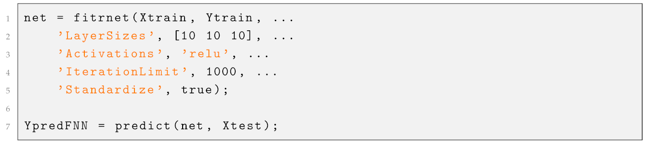
A feedforward neural network was used as the baseline nonlinear memoryless regressor. The model corresponds to a multilayer perceptron with three hidden layers of 10 neurons each and ReLU activations, trained using MATLAB R2025b’s fitrnet function [36,37]. Since each sample is processed independently, the model learns a static nonlinear mapping

$$\hat{y}\left(t\right)=f_{\theta }\left(\mathbf{x}\left(t\right)\right),$$

(1)

where $\hat{y}\left(t\right)$ is the predicted cumulative energy and $\theta$ denotes the network parameters. This formulation does not explicitly incorporate temporal memory, making it a useful baseline for comparison against sequence-aware recurrent models.

The FNN was included to assess whether a static nonlinear relationship between the instantaneous feature vector and cumulative energy is sufficient for this task. As expected, its lack of explicit temporal memory limits its ability to represent the integral and path-dependent nature of cumulative energy. Additional MATLAB R2025b implementation details are provided in Appendix A.

2.3.2. Support Vector Regression (SVR)

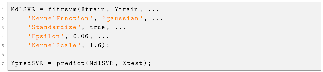
Support Vector Regression was implemented using MATLAB R2025b’s fitrsvm. Based on preliminary experiments, a Gaussian kernel was selected because it yielded lower error than linear and polynomial alternatives on this dataset [38]. The predictor can be written as

$$\hat{y}\left(t\right)=\sum _{i=1}^{N_{\mathrm{sv}}}({\alpha }_i-{\alpha }_i^{\ast })K\left({\mathbf{x}}_i,\mathbf{x}\left(t\right)\right)+b,$$

(2)

where ${\alpha }_i$ and ${\alpha }_i^{\ast }$ are Lagrange multipliers, b is the bias term, and $K(·,·)$ is the Gaussian kernel

$$K({\mathbf{x}}_i,{\mathbf{x}}_j)=exp\left(-{\displaystyle \frac{\parallel {\mathbf{x}}_i-{\mathbf{x}}_j{\parallel }^2}{2{\sigma }^2}}\right).$$

(3)

The kernel scale and $ϵ$-insensitive loss parameter were optimized on the training set, yielding approximately $\mathtt{KernelScale}=1.6$ and $ϵ=0.06$. All input features were standardized before model fitting. This formulation seeks a function that deviates from the true cumulative energy by no more than a prescribed tolerance while maintaining regularization through margin maximization. Additional MATLAB implementation details are provided in Appendix A.

2.3.3. Gaussian Process Regression (GPR)

Gaussian Process Regression was implemented using MATLAB R2025b’s fitrgp with a constant basis function and an exponential covariance kernel [39,40]. GPR treats regression as Bayesian inference over functions, assuming that the latent mapping follows a Gaussian process

$$f\left(\mathbf{x}\right)\sim \mathcal{GP}\left(m\left(\mathbf{x}\right),k(\mathbf{x},{\mathbf{x}}^{\prime })\right),$$

(4)

where $m\left(\mathbf{x}\right)$ is the mean function and $k(\mathbf{x},{\mathbf{x}}^{\prime })$ is the covariance kernel. Observations are modeled as

$$y_i=f\left({\mathbf{x}}_i\right)+{\zeta }_i,$$

(5)

where ${\zeta }_i$ denotes zero-mean Gaussian noise.

Hyperparameters were optimized automatically by maximizing the marginal likelihood on the training data. Output standardization was enabled to improve numerical stability. GPR was included because of its flexibility in modeling nonlinear relationships and its strong performance in several BEV energy-prediction studies, although in this work only point predictions were analyzed. Additional MATLAB implementation details are provided in Appendix A.

2.3.4. Quantile Regression Neural Network (QRNN)

In addition to standard mean regression, a quantile regression approach using neural networks (fitrqnet in MATLAB) was explored. In particular, for E estimation the QRNN uses a loss to estimate a target quantile $\gamma$ [41,42].

The QR loss function, known as pinball loss, penalizes the residuals as follows:

$${\rho }_{\gamma }\left(u\right)=\left\{\begin{array}{cc}\gamma ·u,\hfill & \mathrm{if}u\ge 0,\hfill \\ (\gamma -1)·u,\hfill & \mathrm{if}u<0.\hfill \end{array}\right.$$

(6)

where $\gamma \in (0,1)$ is the desired quantile and $u=y-f\left(x\right)$ is the prediction error.

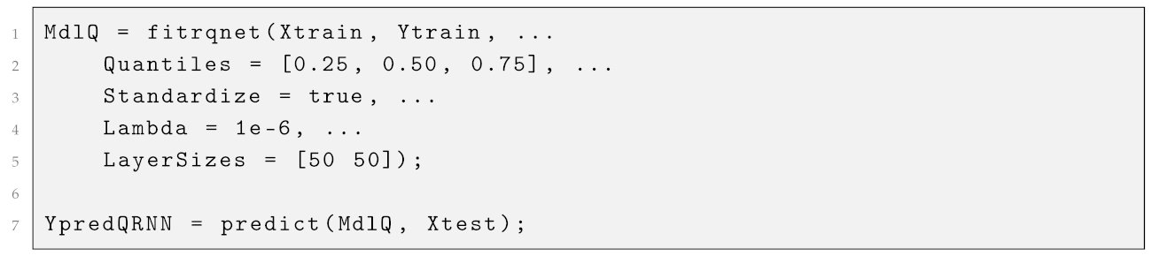
Specified quantiles (e.g., 25th, 50th, 75th percentiles) of the target distribution, instead of just the mean, can be predicted by a QRNN. A QRNN with two hidden layers of 50 neurons each was configured to estimate three quantiles of cumulative energy: 0.25, 0.50 (median), and 0.75. A small L2 regularization term ($\lambda ={10}^{-6}$) was used to improve generalization. The purpose of this model was to assess whether quantile-based prediction could provide additional robustness and uncertainty awareness beyond standard point regression.

For quantitative comparison, the median prediction (QRNN-50) was used as the main point estimate of cumulative energy. Although quantile regression can capture predictive spread, in the present application the target variable is a deterministic cumulative physical quantity, so the median is expected to behave similarly to a conventional central prediction. Additional MATLAB implementation details are provided in Appendix A.

2.3.5. Bagged Trees

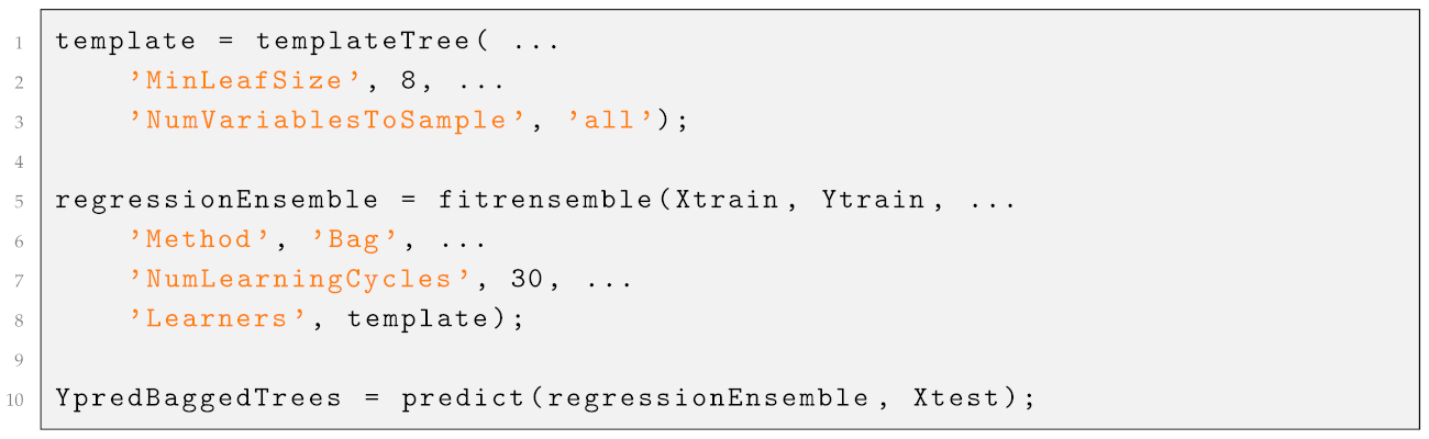
An ensemble regression model based on bagged decision trees was implemented using MATLAB R2025b’s fitrensemble. Thirty regression trees were combined, each trained on a bootstrap subset of the training data. A template tree with minimum leaf size equal to 8 was used, and all five available input features were allowed for splitting in order to maximize information usage.

Bagging reduces prediction variance by averaging multiple low-bias base learners trained on resampled datasets. In this study, the model is referred to consistently as Bagged Trees. This method was included because tree-based ensembles have shown competitive performance in BEV energy modeling and often provide a strong static baseline, especially when nonlinear interactions among predictors are present. Additional MATLAB implementation details are provided in Appendix A.

It is noted that Bagged Trees like random forests have been successfully applied in BEV energy modeling and often rank among top performers in comparisons, though larger training sets might be required for their full potential to be realized.

2.4. Sequence Models (LSTM, GRU, and BiLSTM)

The recurrent models evaluated in this study include a standard Long Short-Term Memory (LSTM) network, a Gated Recurrent Unit (GRU) network, and a Bidirectional Long Short-Term Memory (BiLSTM) network. These architectures were selected because cumulative energy is a path-dependent quantity whose value at time t depends on the preceding sequence of operating states rather than on a single instantaneous observation.

All sequence models were trained in a many-to-one configuration, where an input window of length $T_w$ is mapped to a single cumulative-energy target at the final time step of the window. This design allows the networks to exploit temporal context and learn the progressive accumulation process underlying BEV energy consumption. Additional MATLAB implementation details are provided in Appendix A. The models used are defined below:

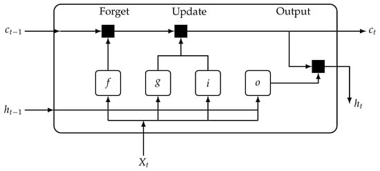
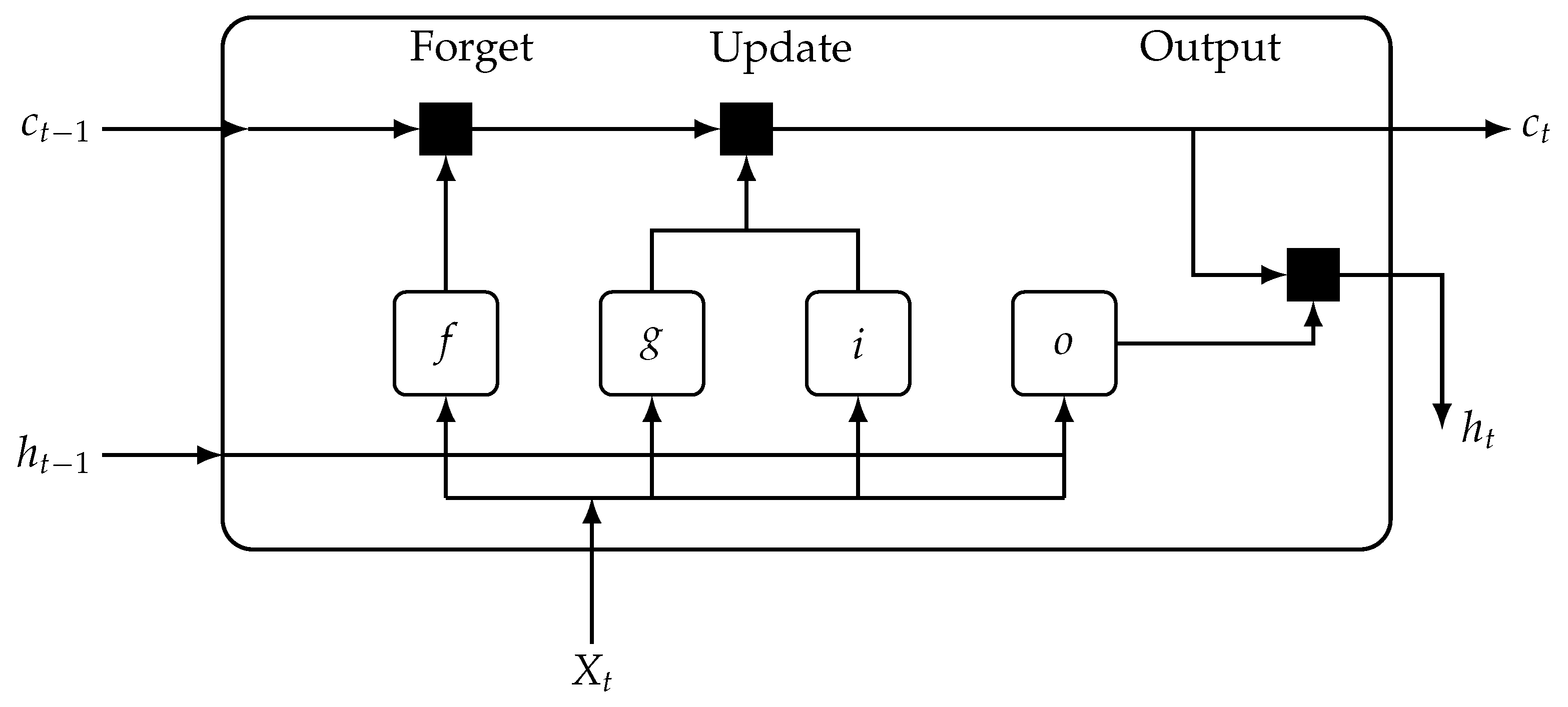
• LSTM (Long Short-Term Memory): A type of recurrent neural network designed to overcome the vanishing gradient problem, capable of learning long-term dependencies in sequential data through the use of a gated cell state [43,44]. The diagram presented in Figure 6 illustrates the data flow in the time unit t. This diagram shows how the gates forget, update, and generate cell and hidden states.

Figure 6. Schematic of a Long Short-Term Memory (LSTM) cell: forget, update, and output stages.

where $h_t$ denotes the hidden state (i.e., the output of the LSTM unit) and $c_t$ denotes the internal cell state at time step t. As illustrated in Figure 6, f, i, c, and o represent the forget gate, input gate, candidate cell state, and output gate, respectively.

• GRU (Gated Recurrent Unit): A simplified variant of the LSTM that also uses gating mechanisms to control the flow of information, but with a more streamlined architecture using fewer gates (update and reset gates) [45,46].
• BiLSTM (Bidirectional Long Short-Term Memory): An extension of the standard LSTM that processes sequence data in both forward and backward directions, allowing the network to capture contextual information from both past and future time steps relative to any point in the sequence [15,47].

These networks take as input a sequence of feature vectors and output a single prediction for the energy at the end of the sequence. By sliding this window across the time series, we can train on many overlapping subsequences from the route. The architecture and training procedure for these sequence models were as follows.

2.4.1. Data Preparation for Sequence Models

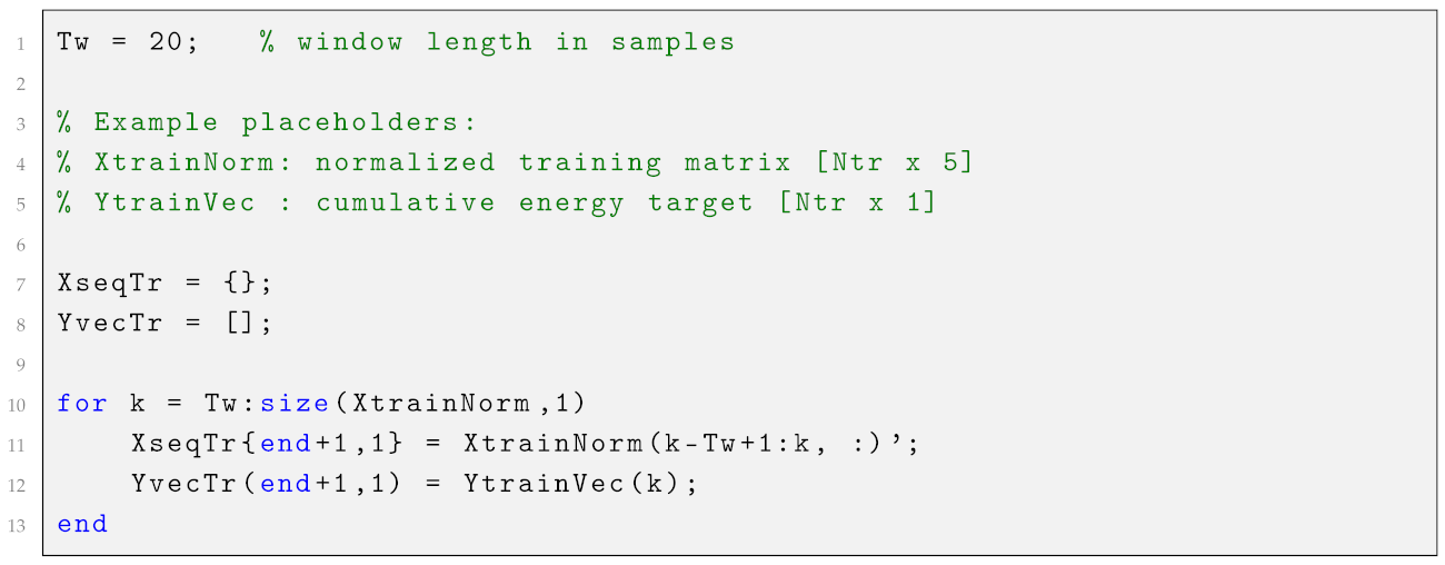
The normalized training data were transformed into multiple shorter sequences using a sliding window of length $T_w=20$ time steps (20 s). Feature normalization was performed using the statistics of the training subset only. For each feature j, the standardized value was computed as

$${\tilde{x}}_{t,j}={\displaystyle \frac{x_{t,j}-{\mu }_j^{\mathrm{tr}}}{{\sigma }_j^{\mathrm{tr}}}},$$

(7)

where ${\mu }_j^{\mathrm{tr}}$ and ${\sigma }_j^{\mathrm{tr}}$ denote the mean and standard deviation of feature j computed from the training set. The same parameters were then applied unchanged to the test set.

The resulting input–target pairs follow a many-to-one formulation:

$${\mathbf{X}}_t=\left[\mathbf{x}(t-T_w+1),\dots ,\mathbf{x}\left(t\right)\right]\in {\mathbb{R}}^{T_w\times 5},\hat{y}\left(t\right)=f_{\theta }\left({\mathbf{X}}_t\right),$$

(8)

where ${\mathbf{X}}_t$ is the input sequence and $y\left(t\right)$ is the cumulative energy at the final time step of the window.

For validation, 15% of the training sequences were held out to monitor validation loss during training. This validation split is distinct from the 30% route-level test set, which remained completely unseen until final evaluation. Test sequences were generated using only test-set observations, thereby preventing information leakage across partitions. Additional MATLAB implementation details are provided in Appendix A.

2.4.2. LSTM Network

To model temporal dependencies in the driving data, the input signals were organized into fixed-length sliding windows of size $T_w=20$. Thus, each training sequence consists of 20 consecutive samples $\left\{X\right(t),X(t+1),\dots ,X(t+19\left)\right\}$, and the network is tasked with predicting the cumulative energy $Y(t+19)$ at the final time step. This formulation corresponds to a many-to-one sequence regression problem.

The window length $T_w=20$ was selected as a trade-off between capturing sufficient temporal context and maintaining computational efficiency during training. Additional experiments with $T_w=10$ and $T_w=30$ yielded similar performance trends, confirming that 20 samples provide an adequate representation of short-term driving dynamics. For each route, approximately $N_{\mathrm{tr}}-T_w$ training sequences were generated, where $N_{\mathrm{tr}}$ denotes the number of training samples. During training, the order of the sequences was randomized to improve generalization; however, the temporal structure within each sequence was strictly preserved.

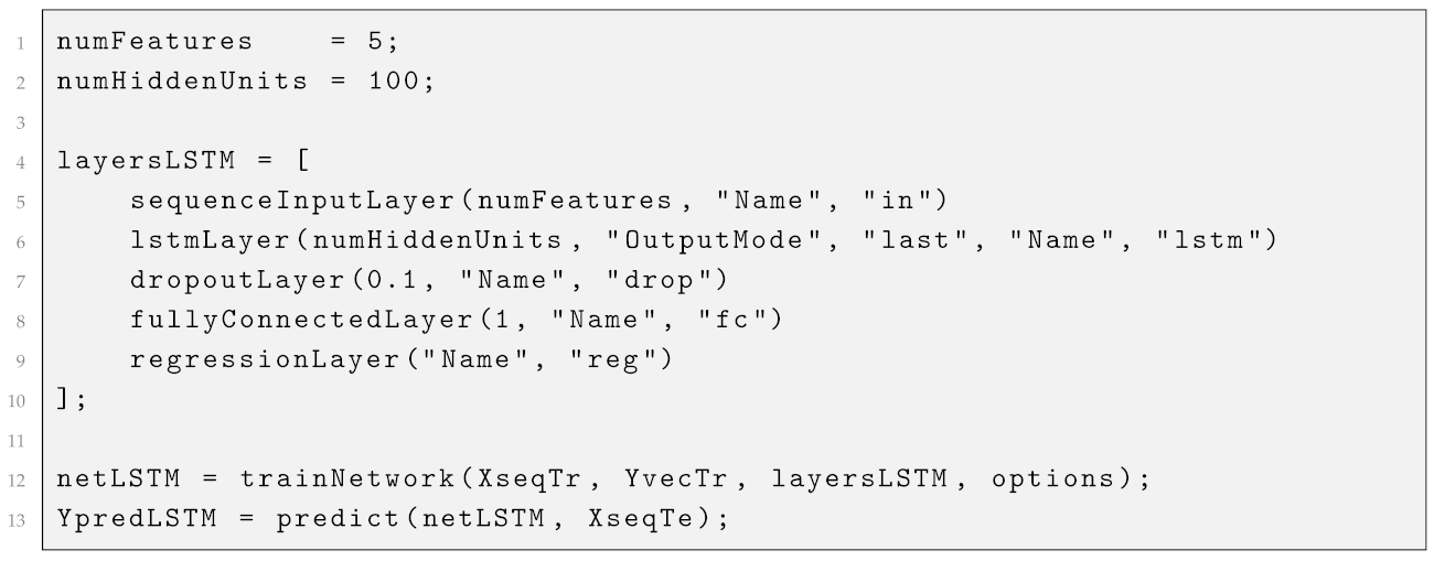
The unidirectional LSTM architecture comprises an input layer for the five features, followed by a single LSTM layer with 100 hidden units. A dropout layer with a rate of 10% was included to mitigate overfitting, and a fully connected layer with a single neuron performs the regression task, followed by a regression output layer. The LSTM layer was configured to output only the last time step, consistent with the many-to-one formulation.

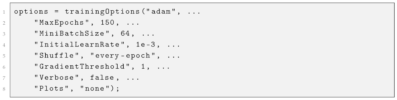
Training was conducted using the Adam optimizer with a learning rate of ${10}^{-3}$, a mini-batch size of 64 sequences, and a maximum of 100 epochs. Although early stopping was not strictly required due to stable convergence of the loss, the validation set was used to monitor potential overfitting and select the best-performing model. Training was repeated multiple times to ensure robustness of the results, and the final performance was evaluated on the test set.

LSTM networks are well suited for capturing long-term temporal dependencies through gated cell states that regulate information flow. In the present application, the model can learn to accumulate the effects of sustained positive motor torque, prolonged acceleration, or persistent uphill altitude changes on cumulative energy consumption.

2.4.3. GRUNetwork

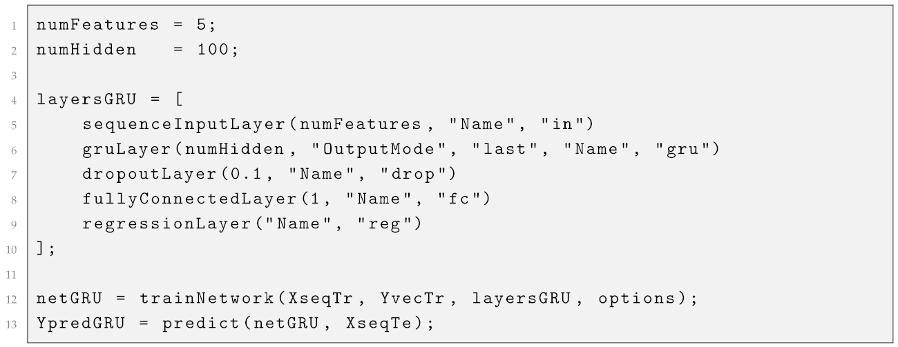
The GRU model has an architecture similar to that of the LSTM, except that the recurrent layer uses Gated Recurrent Unit cells with 100 hidden units and outputs only the last time step. GRUs merge the forget and input gates of an LSTM into a single update gate and simplify the cell-state mechanism, which often leads to faster training and lower computational cost while preserving strong temporal modeling capability.

GRUs merge the forget and input gates of an LSTM into a single update gate and simplify the cell state, which often leads to faster training while retaining comparable sequence modeling power. We trained the GRUnetwork under the same hyperparameters (100 epochs, Adam, etc.) as the LSTM. In the literature, GRUs have sometimes shown slightly better generalization on smaller datasets due to their simpler structure that mitigates overfitting [48]. Although the recurrent layer is implemented using GRU cells, the model is denoted here as GRUto maintain naming consistency with the comparative sequence-learning framework adopted in this study. This designation should therefore be interpreted as a GRU-based recurrent regression model rather than as a hybrid GRUarchitecture.

2.4.4. Bidirectional LSTM

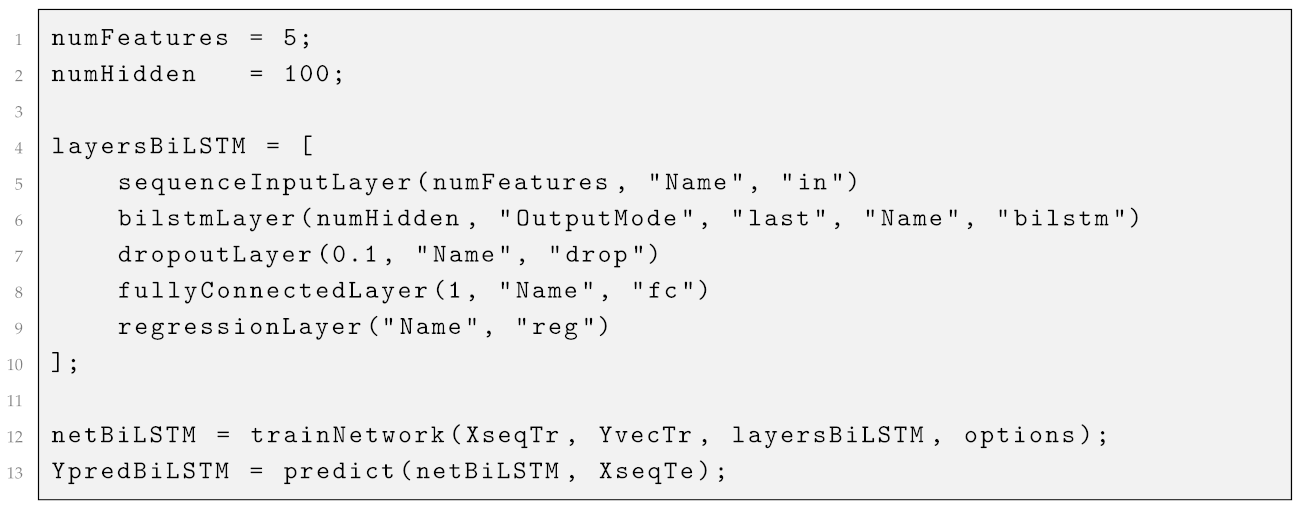
The BiLSTM network doubles the LSTM architecture to process each sequence in both forward and backward directions [49,50,51]. Our BiLSTM layer had 100 hidden units in each direction (so effectively 200 units total), with their outputs concatenated and fed through a dropout and fully connected regression layer similar to the unidirectional case. The BiLSTM can utilize future data within a sequence in addition to past data—for example, when predicting energy at time $t+19$, it considers not only the history from t to $t+19$ (as a forward LSTM would) but also backwards context starting from $t+19$ and going to t. This is beneficial for off-line predictions or when the entire sequence is known. We trained the BiLSTM with the same procedure as above. We denote this model as BiLSTM in the results to maintain naming consistency within the comparative recurrent-model framework adopted in this study. BiLSTM networks have been reported to achieve higher accuracy in capturing temporal patterns because they effectively see the sequence twice (forward and backward), which can capture relationships that a single-direction RNN might miss.

2.5. Performance Metrics and Evaluation

All models were evaluated on an independent test set comprising 30% of the samples from each route. Model performance was primarily assessed using the root mean square error (RMSE) and the coefficient of determination (R²), which together provide complementary insights into prediction accuracy and goodness of fit. In selected cases, the mean absolute error (MAE) was also reported to provide additional interpretability of absolute prediction deviations.

The RMSE measures the average magnitude of the prediction error in the same physical units as the target variable (kWh) and is defined as

$$\mathrm{RMSE}=\sqrt{{\displaystyle \frac{1}{N}}\sum _{i=1}^N{\left(Y_i^{\mathrm{pred}}-Y_i^{\mathrm{true}}\right)}^2}.$$

(9)

The coefficient of determination R² quantifies the proportion of variance in the true energy consumption explained by the model and is computed as

$$R^2=1-{\displaystyle \frac{{\displaystyle \sum _{i=1}^N}{\left(Y_i^{\mathrm{pred}}-Y_i^{\mathrm{true}}\right)}^2}{{\displaystyle \sum _{i=1}^N}{\left(Y_i^{\mathrm{true}}-{\overline{Y}}^{\mathrm{true}}\right)}^2}},$$

(10)

where ${\overline{Y}}^{\mathrm{true}}$ denotes the mean of the true test values. An R² value of 1 indicates a perfect fit, while a value of 0 indicates that the model performs no better than predicting the mean of the target variable.

The mean absolute error (MAE), which provides a direct measure of the average absolute deviation between predictions and ground truth, is defined as

$$\mathrm{MAE}={\displaystyle \frac{1}{N}}\sum _{i=1}^N\left|Y_i^{\mathrm{pred}}-Y_i^{\mathrm{true}}\right|.$$

(11)

Since each driving route differs in length, driving dynamics, and energy consumption range, all models were trained and evaluated independently on each route (within-route training and testing). Route 1 was selected as the representative case for detailed visualization because it combines mixed urban operation, hilly topography, and a moderate sequence length of 1917 samples, making it suitable for illustrating both the input-variable evolution and the cumulative-energy prediction task.

To ensure a fair comparison, all models were trained using identical training indices and evaluated on the same test samples for each route. Variability due to random weight initialization in neural networks was mitigated by averaging results over multiple runs when necessary. For qualitative comparison, predicted energy consumption time series are plotted against the corresponding ground truth for selected models, and the test RMSE of all models is summarized in a single comparative figure. Figure 1 (see Section 3) presents a bar chart of the RMSE values for the eight principal models evaluated in this study: MLP, SVR, GPR, QRNN (median), Bagged Trees, LSTM, GRU, and BiLSTM.

3. Results

3.1. Overall Comparison on a Representative Route

We first present detailed comparative results for Route 1 as a representative benchmark case. Table 2 summarizes the test performance of all evaluated models on this route.

Table 2. Results Route 1.

Model	Test RMSE (kWh)	Test R2	Test MAE (kWh)
FNN	0.1973	0.9295	0.1147
SVR	0.1949	0.9312	0.1211
GPR	0.1821	0.9399	0.1019
QRNN 50%	0.1791	0.9419	0.0949
Bagged Trees	0.1718	0.9465	0.0850
LSTM	0.2992	0.8224	0.1302
GRU	0.0909	0.9836	0.0588
BiLSTM	0.1458	0.9578	0.0885

3.2. Analysis of Specific Models

To better understand the strengths and limitations of each approach, we provide some additional observations:

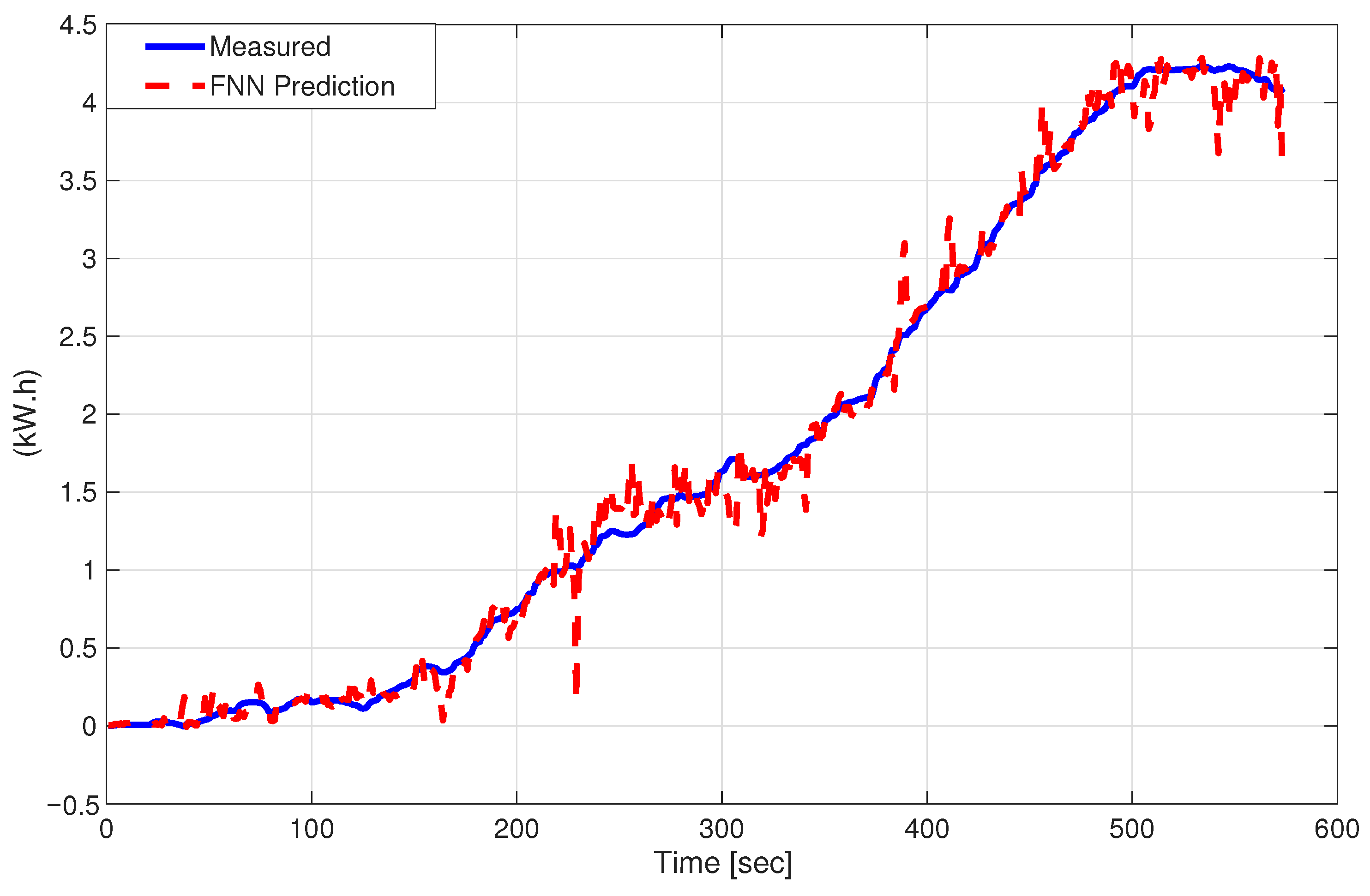
• FNN: With only instantaneous inputs, FNN exhibited systematic lag during high-slope segments of the cumulative energy curve (Figure 7), confirming the insufficiency of memoryless mappings for integral quantities. Its performance was only slightly better than a naive baseline (predicting mean energy). This indicates that a static nonlinear mapping from [Speed, Accel, Torque, Altitude, Pedal] to Energy is insufficient—as expected, the problem inherently requires memory of past events (distance traveled, etc.). Figure 7 shows that the FNN captures the monotonic trend of cumulative energy, but its memoryless structure leads to visible lag during rapidly changing segments.
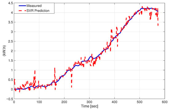
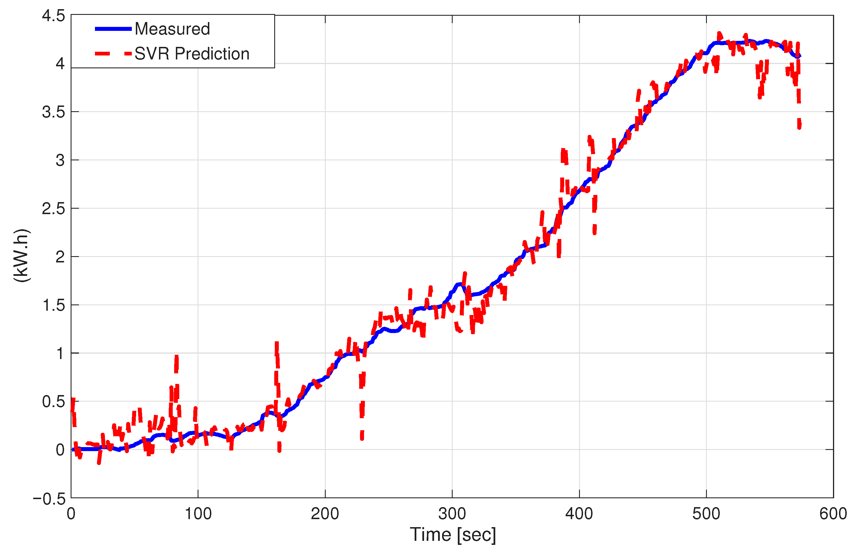
• SVR (Gaussian Kernel): The SVR captured nonlinearities better than the MLP and showed reasonable performance on some routes, especially those that were flatter (energy roughly proportional to distance). However, on routes with varying terrain or stop-and-go driving, the SVR had difficulty. It cannot seamlessly model the piecewise linear growth of energy with occasional plateaus (regenerative braking periods) without temporal input. The SVR’s error was typically 1.5–2 times that of the best LSTM model. Figure 8 shows that SVR improves the nonlinear fit relative to the FNN, although it still struggles to reproduce local route-dependent variations without temporal context.
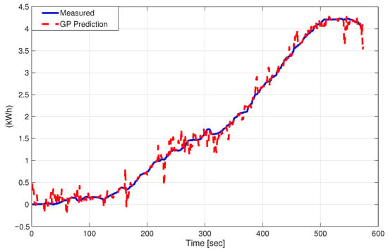
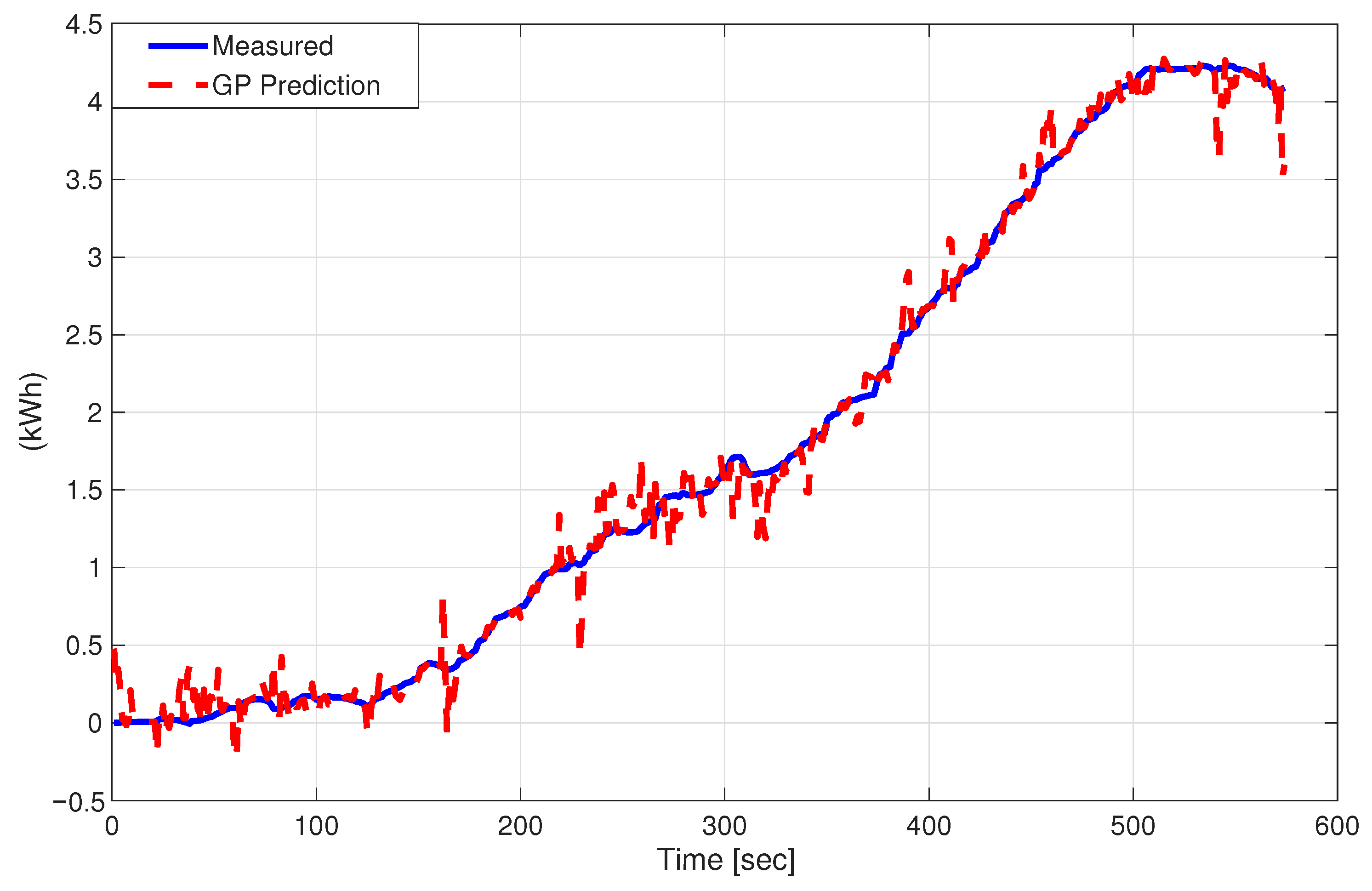
• Gaussian Process (Exponential kernel):Gaussian Process Regression (GPR) was the strongest among the memoryless models on several routes, consistently outperforming FNN and SVR. Its flexibility likely allowed it to capture smooth nonlinear relationships between vehicle dynamics and cumulative energy, particularly under less abrupt driving profiles. However, its performance remained below that of recurrent architectures in the most dynamic routes, highlighting the limitations of static regression when the target variable is inherently path-dependent. Figure 9 shows that GPR provides a smoother static approximation of the cumulative energy trajectory, but remains limited in highly dynamic sections.
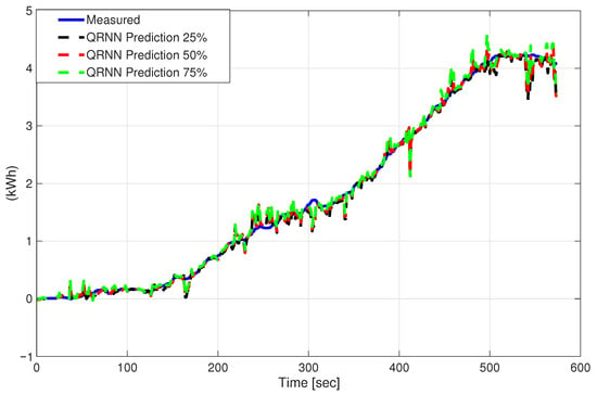
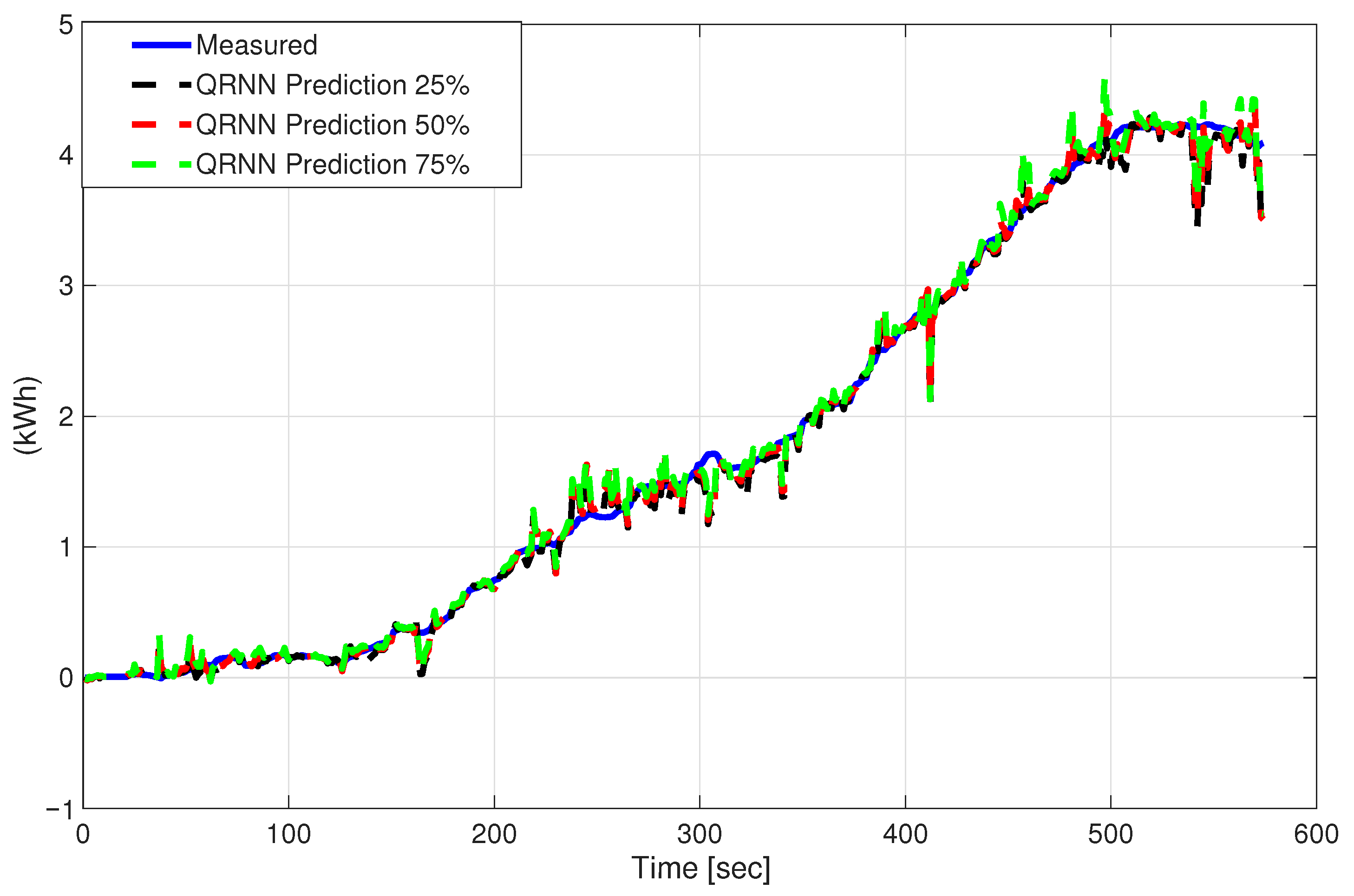
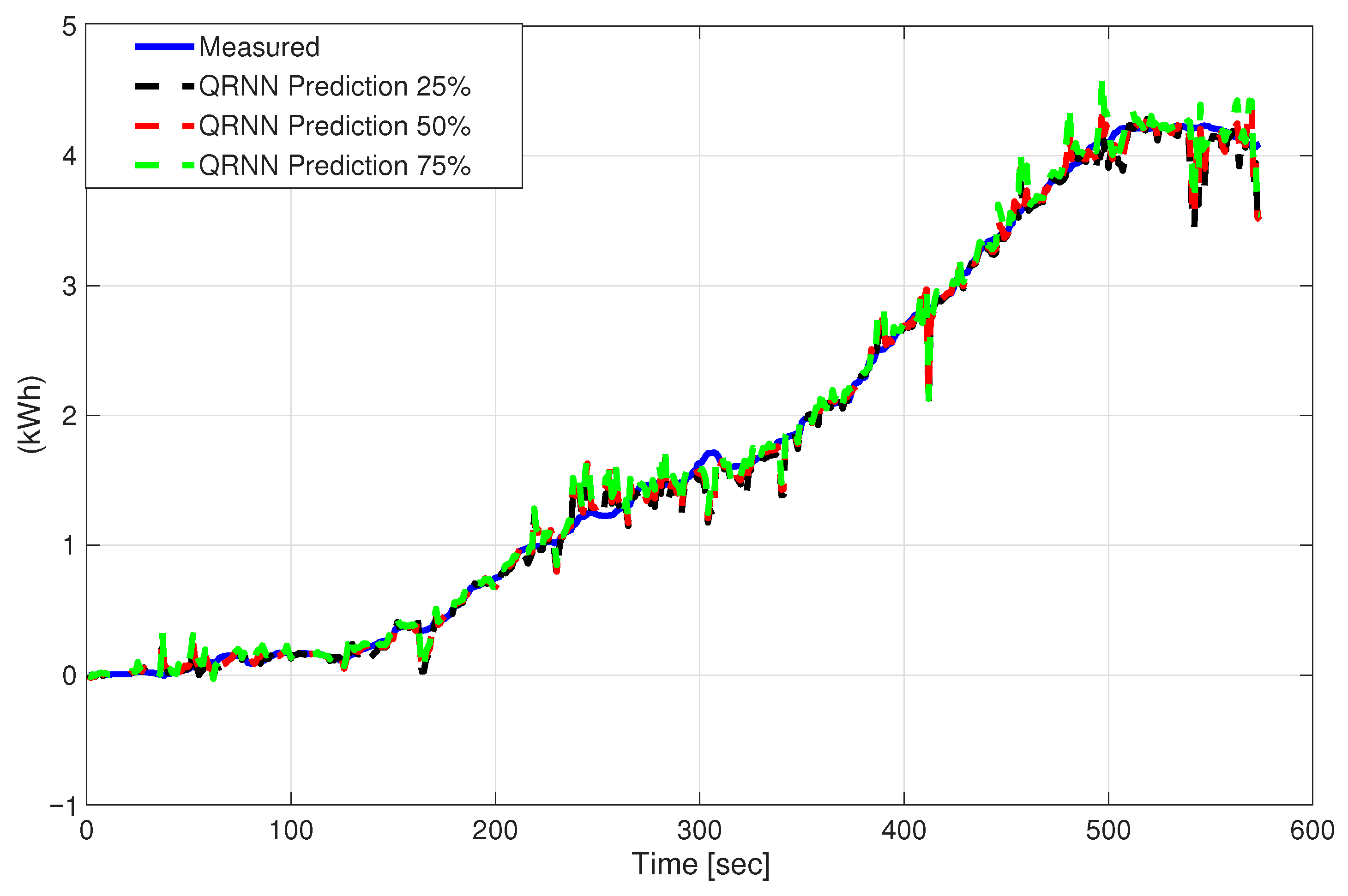
• Quantile Regression NN: The QRNN’s median predictions were similar in accuracy to the MLP. Interestingly, the spread between its 25th and 75th quantile outputs provided a reasonable prediction interval for the energy curve. We observed that the true energy usually stayed within the QRNN-predicted 25–75% band, widening during periods of rapid change. This suggests the QRNN could be useful if one needs uncertainty bounds (for instance, for risk-averse energy management). However, for point prediction, it did not outperform the standard neural network, likely because optimizing quantile loss is a harder problem than MSE for a single output. Figure 10 shows that the QRNN is useful not only for median prediction, but also for visualizing uncertainty through the interquantile band.
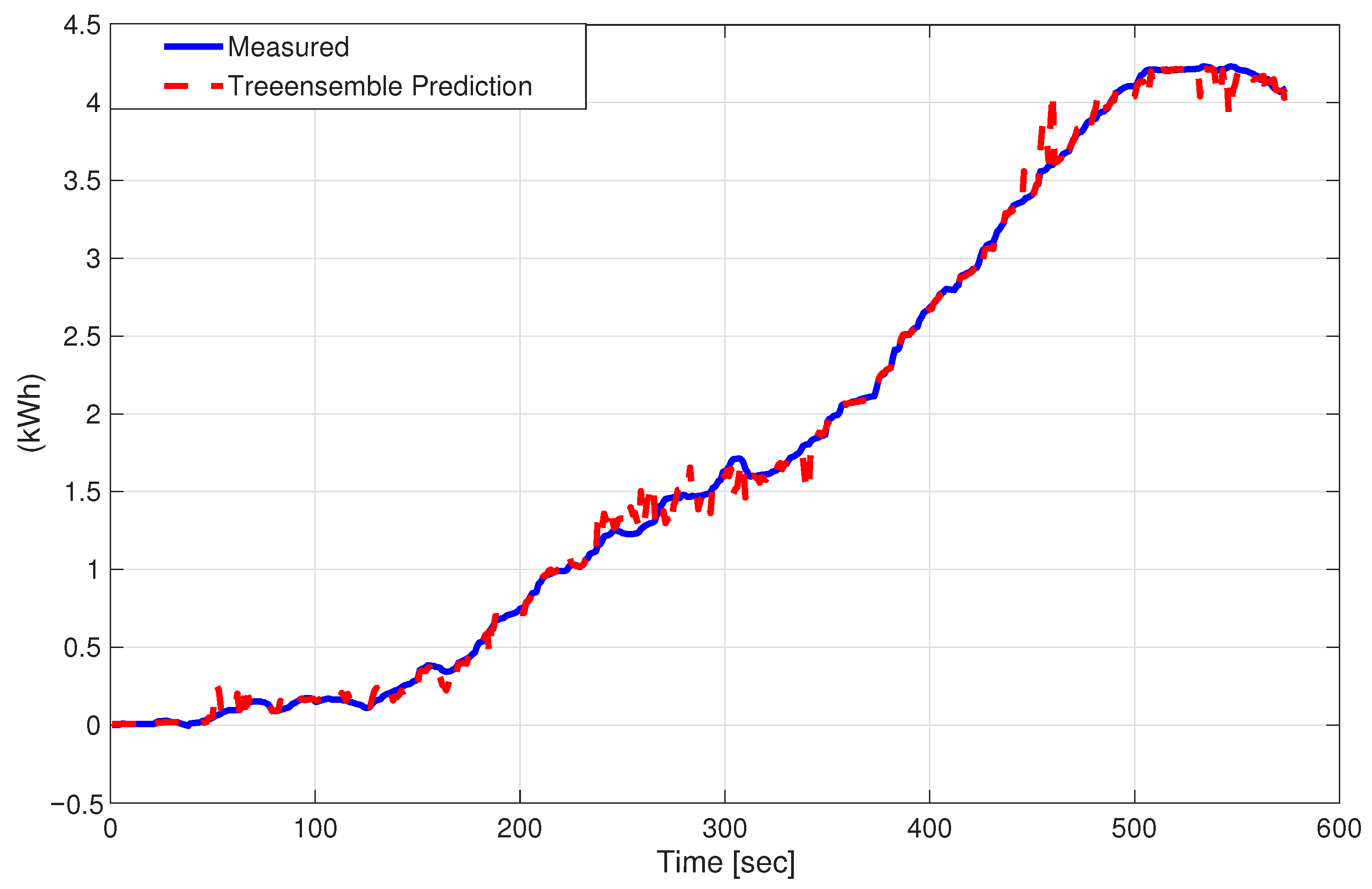
• Bagged Trees (Bagging): The bagged trees performed well given their simplicity, ranking just below GPR on most routes. They captured some nonlinearity (for example, they could model different energy increase rates in different ranges of speed or torque). The ensemble’s predictions were somewhat noisier, and we noticed occasional jumps or plateaus from individual trees. Smoothing could help, but that risks bias. Notably, in the absence of temporal features, the Bagged Trees effectively did piecewise constant approximations. If the vehicle had very repetitive behavior, the trees might memorize that after a certain altitude and speed combination usually the energy is a certain amount. But for unique scenarios, they err. Bagged Treess are known to require sufficient data covering all patterns; in small routes, they might miss some combinations. This is consistent with the literature noting that with limited data, simpler or ensemble models can be robust but might lack the fine temporal resolution that RNNs provide.Figure 11 shows that Bagged Trees provides a competitive static baseline for Route 1, although its piecewise predictions still reveal the absence of explicit temporal memory.
• LSTM vs. GRU vs. BiLSTM: The sequence-based architectures (GRU and BiLSTM) consistently outperformed memoryless regression models across most evaluated routes. As shown in Table 2, the Bagged Trees achieved the lowest RMSE on Route 1, demonstrating that static models can occasionally excel when route-specific patterns align favorably. However, the comparative results presented in Table 3, Table 4 and Table 5, indicate that recurrent models dominate performance across the remaining nine routes, particularly those characterized by higher dynamic variability. This overall trend confirms that incorporating temporal context is essential for accurately modeling cumulative energy dynamics. Figure 12 compares the three recurrent architectures and shows that sequence-aware models follow the measured cumulative energy curve more closely than the memoryless regressors in this representative route.

Figure 7. Measured and predicted cumulative energy for Route 1 using the feedforward neural network (FNN). The figure shows that the memoryless nonlinear mapping captures the global increasing trend but exhibits visible lag and local mismatch during segments with rapid changes in slope, highlighting the limitation of instantaneous-input models for cumulative energy estimation.

Figure 8. Measured and predicted cumulative energy for Route 1 using support vector regression (SVR) with a Gaussian kernel. The model reproduces the overall nonlinear growth pattern more accurately than the FNN but still shows limited ability to track local slope changes and plateau-like regions associated with dynamic driving behavior.

Figure 9. Measured and predicted cumulative energy for Route 1 using Gaussian process regression (GPR) with an exponential kernel. The figure illustrates that GPR provides a smoother approximation of the cumulative energy trajectory than other static regressors, although localized deviations remain visible in segments with stronger transient dynamics.

Figure 10. Measured and predicted cumulative energy for Route 1 using the median output of the quantile regression neural network (QRNN-50). The predicted profile follows the measured trajectory with improved smoothness relative to conventional memoryless models, although it still lacks the temporal adaptability required to consistently reproduce all route-dependent variations.

Figure 11. Measured and predicted cumulative energy for Route 1 using the Bagged Trees model. The ensemble captures the overall route-level consumption trend with competitive accuracy, but small staircase-like deviations and local plateaus remain visible, reflecting the piecewise approximation behavior of tree-based regression without explicit temporal memory.

Table 3. RMSE of energy consumption prediction from models developed using different routes for the electric vehicle.

ROUTES	Model
	FNN	SVR	GPR	QRNN 50%	Tree	LSTM	GRU	BiLSTM
1	0.1973	0.1949	0.1821	0.1791	0.1718	0.2992	0.0909	0.1458
2	0.1016	0.1695	0.1305	0.1097	0.0879	0.2247	0.0986	0.1224
3	0.1495	0.1721	0.1441	0.1321	0.1430	0.2295	0.0496	0.1055
4	0.1366	0.1686	0.1329	0.1250	0.1176	0.3283	0.0929	0.1084
5	0.2138	0.2680	0.2166	0.2211	0.1675	0.3457	0.1784	0.1856
6	0.3430	0.3991	0.3543	0.3316	0.2986	0.2520	0.1883	0.1472
7	0.0474	0.0652	0.0528	0.0531	0.0674	0.0593	0.0385	0.0648
8	0.1525	0.1995	0.1479	0.1611	0.1161	0.2036	0.1571	0.1540
9	0.0918	0.2444	0.1504	0.0767	0.1102	0.2024	0.0670	0.0703
10	0.5070	0.3911	0.3118	0.3198	0.2743	0.4340	0.1815	0.2007

Table 4. R² of energy consumption prediction from models developed using different routes for the electric vehicle.

ROUTES	Model
	FNN	SVR	GPR	QRNN 50%	Tree	LSTM	GRU	BiLSTM
1	0.9295	0.9312	0.9399	0.9419	0.9465	0.8224	0.9836	0.9578
2	0.9954	0.9871	0.9924	0.9946	0.9924	0.9770	0.9956	0.9932
3	0.8638	0.8194	0.8735	0.8936	0.8754	0.6847	0.9853	0.9333
4	0.9913	0.9868	0.9918	0.9917	0.9732	0.9490	0.9959	0.9944
5	0.6251	0.4110	0.6151	0.5991	0.6966	0.3852	0.8389	0.8267
6	0.8763	0.8325	0.8680	0.8844	0.9062	0.9357	0.9641	0.9781
7	0.8736	0.7614	0.8433	0.8417	0.9275	0.7763	0.9056	0.8632
8	0.9908	0.9843	0.9914	0.9898	0.8947	0.9831	0.9920	0.9903
9	0.9486	0.6358	0.8621	0.9641	0.9260	0.7578	0.9735	0.9708
10	0.3386	0.6064	0.7499	0.7369	0.8065	0.4939	0.9115	0.8918

Table 5. MAE of energy consumption prediction from models developed using different routes for the electric vehicle.

ROUTES	Model
	FNN	SVR	GPR	QRNN 50%	Tree	LSTM	GRU	BiLSTM
1	0.1147	0.1211	0.1019	0.0949	0.0850	0.1302	0.0588	0.0885
2	0.0649	0.1070	0.0751	0.0590	0.0437	0.1269	0.0764	0.0960
3	0.0736	0.1134	0.0813	0.0702	0.0790	0.1143	0.0343	0.0605
4	0.0854	0.1090	0.0769	0.0631	0.0843	0.1763	0.0747	0.0872
5	0.1070	0.1488	0.1152	0.1090	0.1105	0.1558	0.0932	0.0856
6	0.1786	0.2163	0.1549	0.1434	0.1400	0.1540	0.0990	0.0863
7	0.0278	0.0564	0.0323	0.0324	0.0478	0.0453	0.0289	0.0432
8	0.0985	0.1229	0.0831	0.0935	0.1171	0.1367	0.1096	0.0811
9	0.0550	0.1436	0.0789	0.0470	0.0588	0.1174	0.0493	0.0504
10	0.3102	0.2526	0.2003	0.1806	0.1685	0.1948	0.1002	0.1092

Figure 12. Measured and predicted cumulative energy for Route 1 using the three sequence-aware recurrent models evaluated in this study: LSTM, GRU, and BiLSTM. All recurrent architectures track the measured trajectory more closely than the memoryless regressors, with the GRU and BiLSTM variants showing better agreement than the standard LSTM in this representative route, thereby illustrating the value of temporal context for cumulative energy prediction.

Among the recurrent architectures, the BiLSTM exhibited a marginal yet consistent advantage in several high-dynamic scenarios, reducing RMSE by approximately 5–10% relative to the unidirectional LSTM. This improvement can be attributed to the bidirectional processing of temporal information within each window, which enhances the network’s ability to capture contextual dependencies in highly dynamic driving conditions. The BiLSTM’s ability to consider future context within a sequence likely helps it better fit the end-of-window energy. However, it is important to note that BiLSTM is not causal—it uses data from ahead of the prediction point—which precludes its use in real-time prediction scenarios. For live range estimation, a unidirectional LSTM or GRUremains the more appropriate choice, whereas BiLSTM is well-suited for offline analysis and planning applications.

A noteworthy exception appears in Route 1, where the standard LSTM yielded a markedly higher error than both the GRU-based model and the BiLSTM variant. This behavior suggests route-specific sensitivity of the plain LSTM to optimization dynamics under medium-scale data and strongly varying local transients. Route 1 combines urban stop-and-go behavior with pronounced elevation changes, which may produce temporal patterns that are harder for the standard unidirectional LSTM to fit consistently. In contrast, the GRU-based model likely benefited from its simpler gating structure, while the BiLSTM gained additional contextual information from bidirectional processing within the analysis window. Therefore, this isolated degradation should be interpreted as architecture-dependent training variability rather than as a contradiction of the broader recurrent-model trend observed across the remaining routes.

The GRU model’s performance was largely on par with the LSTM, and in a few routes, GRUeven slightly outperformed its more complex counterpart. This aligns with studies reporting that GRU can match LSTM accuracy with fewer parameters, offering a favorable trade-off between computational efficiency and predictive power. Both LSTM and GRUdemonstrated high accuracy in tracking the energy curve, with R² values frequently exceeding 0.95. Qualitative analysis revealed that the trained GRUeffectively learned to integrate acceleration and torque inputs over time a behavior analogous to the physical integration of power. During coasting or regenerative braking events (characterized by negative torque), the recurrent models correctly learned to flatten or reduce the energy curve slope, a capability that non-sequence models consistently struggled to replicate. This suggests that the learned cell states encode accumulated energy expenditure, effectively serving as an internal memory of consumption progress along the route.

Overall, the route-level results indicate that sequence-based models provide the most reliable performance for cumulative energy prediction, particularly under dynamically varying driving conditions. Among them, GRU achieved the strongest average performance, whereas Bagged Trees remained the most competitive memoryless alternative, as shown in Table 2.

Additionally, our work highlights that GPR remains a strong contender among classical methods, aligning with studies that found GPR can outperform neural networks in certain BEV energy forecasting tasks. Nevertheless, in our sequential formulation—where temporal dependencies are central GPR was still outshone by recurrent architectures, underscoring the importance of matching model choice to problem structure.

4. Discussion

The results provide strong evidence that cumulative energy prediction in battery electric vehicles is fundamentally a temporal learning problem rather than a purely memoryless regression task. Unlike instantaneous power, cumulative energy is an integral quantity that depends on the trajectory of past operating states. Consequently, models that map only the current driving condition to accumulated energy are inherently limited, particularly under transient and highly dynamic driving patterns. In contrast, recurrent architectures are able to retain and update latent state information over time, allowing them to approximate the integration process that underlies energy accumulation more effectively.

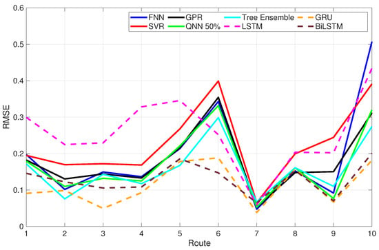
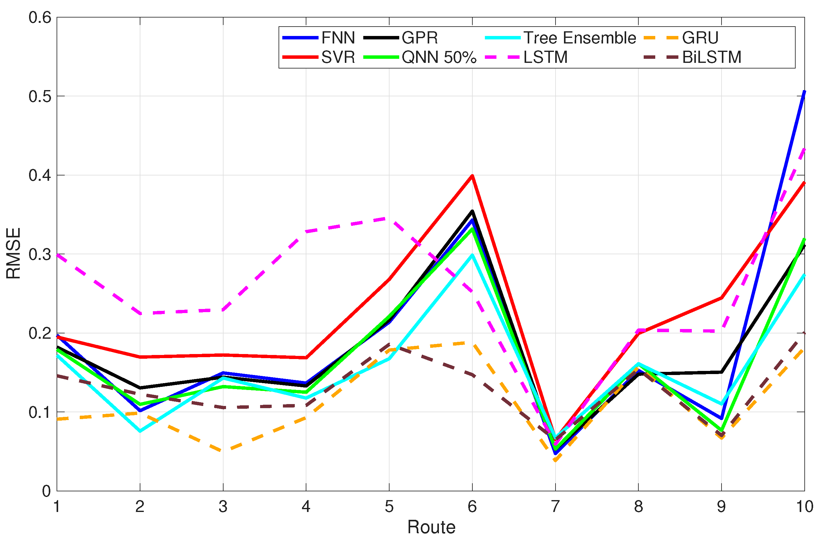
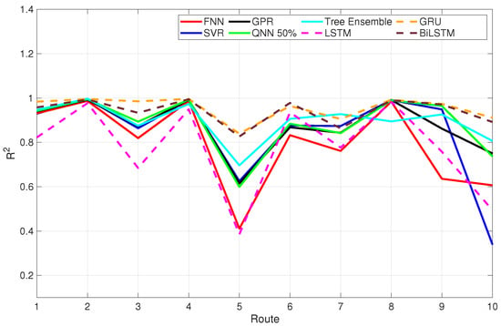
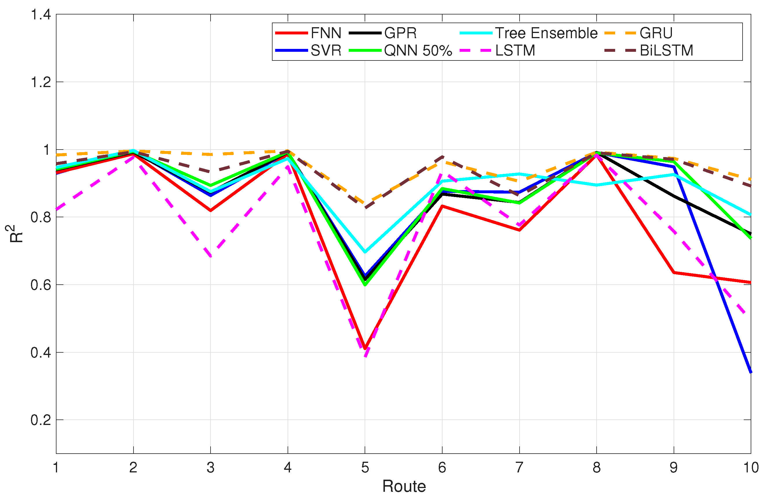
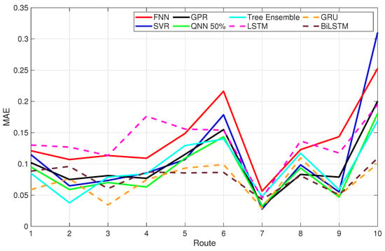
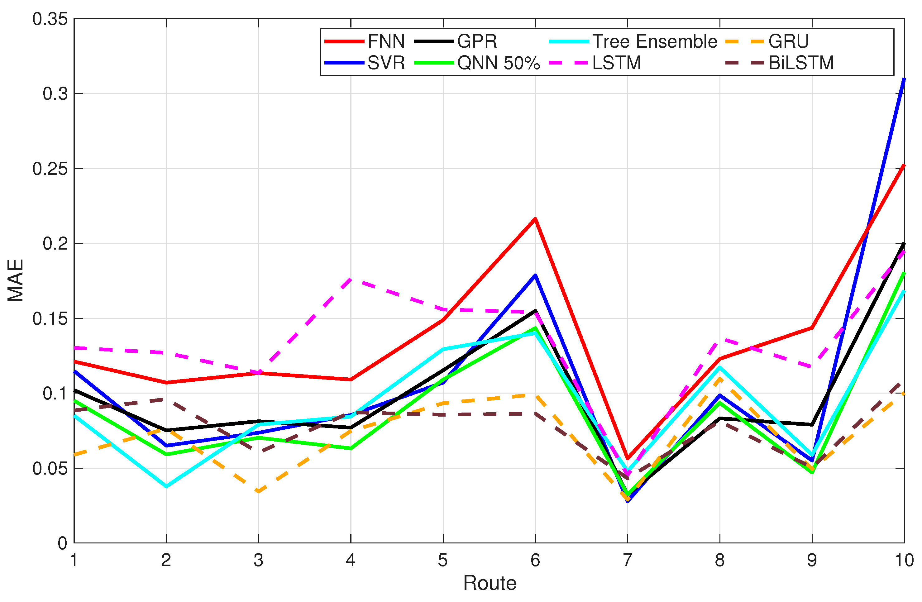
The superior performance of recurrent architectures (LSTM, GRU, and BiLSTM) can be interpreted as an implicit learning of the integration process that governs cumulative energy accumulation. Since energy is mathematically defined as the time integral of power, any accurate predictor must encode a form of temporal memory. Static regressors attempt to approximate this integral through nonlinear mappings of instantaneous inputs; however, without access to prior states, they cannot reconstruct the path-dependent evolution of energy, as can be verified in Table 3, Table 4 and Table 5 and Figure 13, Figure 14 and Figure 15. Figure 13 summarizes the route-wise RMSE obtained by the evaluated models. Figure 14 compares the coefficient of determination across routes and highlights the stronger consistency of the recurrent architectures. Figure 15 complements the error analysis by reporting the route-wise MAE values.

Figure 13. Route-wise RMSE comparison of the evaluated models across the ten driving routes. Lower values indicate better cumulative energy prediction accuracy. The figure shows that sequence-aware recurrent models, particularly GRU and BiLSTM, generally achieve lower error than memoryless regressors, while Bagged Trees remains competitive on several smoother routes.

Figure 14. Route-wise R² comparison of the evaluated models across the ten driving routes. Higher values indicate better agreement between predicted and measured cumulative energy. Recurrent architectures achieve the highest overall explanatory power, with GRU providing the most consistent performance across routes.

Figure 15. Route-wise MAE comparison of the evaluated models across the ten driving routes. This metric highlights the average absolute deviation from the measured cumulative energy profile and confirms the stronger overall robustness of the recurrent models, while static models remain competitive in selected routes with smoother dynamics.

Recurrent networks overcome this limitation by maintaining internal states that evolve over time. In this context, gated memory units act as adaptive accumulators, selectively retaining or forgetting information related to sustained torque demand, prolonged acceleration, or persistent uphill gradients. The empirical results therefore support a theoretical interpretation: cumulative energy estimation is not merely a nonlinear regression problem but a sequence modeling task aligned with dynamic system integration.

Among the recurrent models, GRU delivered the strongest overall performance, suggesting that its simpler gating structure provides an effective balance between representational power and generalization for medium-scale route-level datasets. BiLSTM remained competitive and, in some highly dynamic routes, benefited from access to bidirectional context within the analysis window. However, because this advantage depends on future samples inside the window, its practical relevance is greater for offline analysis than for strictly causal onboard prediction.

Despite the structural advantage of recurrent architectures, Bagged Trees demonstrated competitive performance in several routes, particularly those characterized by smoother dynamics and near-linear energy growth. This finding is important from an implementation standpoint: under quasi-steady driving conditions, cumulative energy behaves approximately as a monotonic function of speed and torque demand, allowing static nonlinear models to approximate the mapping with acceptable accuracy.

Bagged Trees remained competitive in several routes and, in selected scenarios, outperformed SVR and approached the performance of GPR. However, its lack of temporal memory limited its robustness under highly dynamic driving conditions. This can be attributed to the piecewise partitioning nature of decision trees, which enables localized modeling of regime-dependent energy behaviors such as regenerative braking plateaus or torque surges. Without temporal context, however, these models remain limited in capturing longer-range dependencies.

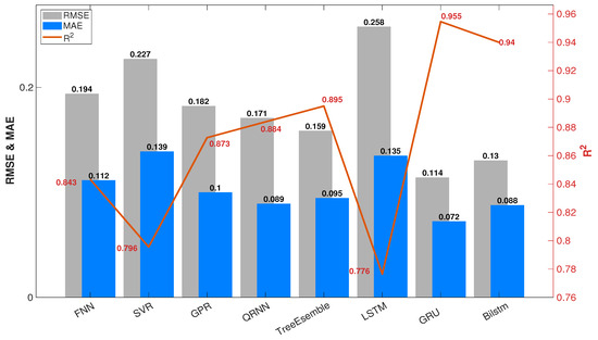
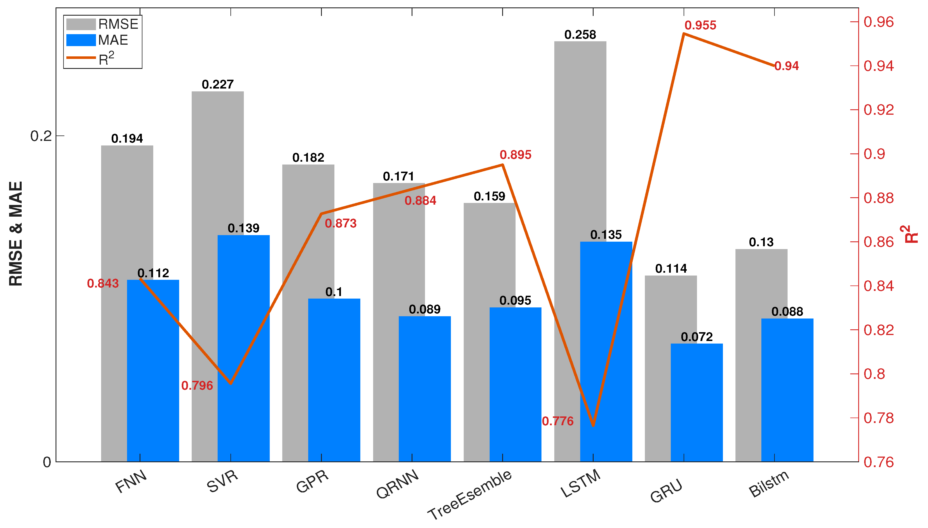
These results clarify inconsistencies often observed in the literature, where Bagged Trees sometimes outperform deep networks in trip-level prediction but underperform in high-resolution cumulative forecasting, as shown in Figure 16. The present benchmark demonstrates that the relative superiority of modeling paradigms depends strongly on whether the prediction target is instantaneous, aggregated, or sequentially accumulated.

Figure 16. Aggregate performance comparison of the evaluated models over the ten driving routes using RMSE, MAE, and R². The figure summarizes the overall ranking of the modeling paradigms and shows that GRU achieves the best global trade-off between accuracy and consistency, followed by BiLSTM and Bagged Trees.

An important practical question is how the observed model differences translate into engineering significance. In this study, the reported errors are expressed in cumulative energy units (kWh), not in normalized specific-consumption units (kWh/km). Therefore, the results should be interpreted as route-level deviations in accumulated energy estimation rather than as direct long-distance extrapolations. From the aggregate comparison across the ten routes, the best-performing GRU model achieved an average RMSE of approximately 0.114 kWh and an MAE of 0.072 kWh, whereas Bagged Trees reached about 0.159 kWh RMSE and 0.095 kWh MAE, and the FNN baseline about 0.194 kWh RMSE and 0.112 kWh MAE. This corresponds to an average RMSE reduction of approximately 28% relative to Bagged Trees and 41% relative to FNN, with similarly meaningful MAE reductions. These differences indicate that the gain of sequence-aware models is not merely marginal, but reflects a practically relevant improvement in cumulative-energy trajectory estimation.

The GRU architecture used in this work consists of a single recurrent layer with 100 hidden units and a lightweight regression head. This configuration provides high predictive fidelity while maintaining modest parameter count and stable training behavior. The findings suggest that medium-complexity recurrent networks strike a practical balance between accuracy and deployability for embedded energy management systems. Furthermore, the controlled benchmarking protocol ensures that performance differences arise from architectural characteristics rather than preprocessing inconsistencies. This methodological fairness strengthens the interpretability of comparative outcomes and provides a reproducible reference framework for future studies.

Previous studies have reported high R² values for trip-level total energy consumption prediction using boosting or transformer-based models. However, many of those works focus on aggregated metrics or end-of-trip estimation. In contrast, this study addresses second-by-second cumulative forecasting, a more stringent and dynamically sensitive task. The results align with prior findings that recurrent neural networks outperform static regressors in time-series energy modeling. However, this work extends that understanding by explicitly formalizing cumulative energy estimation as a many-to-one sequence regression problem aligned with physical integration. This conceptual framing bridges the gap between data-driven learning and underlying vehicle energy dynamics.

Additionally, the benchmark confirms that while sophisticated deep architectures may offer incremental gains, simpler gated recurrent structures can achieve comparable accuracy under realistic route-level conditions.

Several limitations should be acknowledged. First, the evaluation was conducted using intra-route random holdout partitioning. Although care was taken to avoid sequence-level lookahead within each training window, this design does not constitute strict chronological forecasting and cannot fully assess cross-route generalization. Consequently, the superiority of recurrent models observed here should be interpreted within the context of controlled within-route benchmarking. Future work should incorporate temporally ordered splits and leave-one-route-out validation to evaluate temporal robustness and route-to-route transferability under more realistic deployment conditions.

Second, the dataset corresponds to a single vehicle platform operating over ten routes within a specific high-altitude urban context in Cuenca, Ecuador. Although this provides a controlled and internally consistent benchmark, it does not ensure broad representativeness across vehicle types, climates, or geographical regions. Nevertheless, the selected environment is technically meaningful, since reduced air density and local topographical characteristics at approximately 2500 m above sea level may significantly influence BEV energy-consumption dynamics. Broader external validation will therefore require multi-vehicle datasets and geographically diverse operating conditions.

Third, instantaneous electrical variables (current and voltage) were intentionally excluded from predictors to maintain a purely dynamics-based estimation framework. While this isolates the learning challenge, hybrid models incorporating limited electrical measurements may further enhance robustness.

5. Conclusions

Rather than claiming architectural novelty, this work contributes by defining and validating a rigorous benchmark for second-by-second cumulative energy prediction in battery electric vehicles using real-world route data. Under this framework, eight machine learning models were systematically evaluated using 1 Hz telemetry collected from ten real-world driving routes, including five memoryless regression approaches (FNN, SVR, GPR, QRNN, and Bagged Trees) and three sequence-based architectures (LSTM, GRU, and BiLSTM), all assessed under identical preprocessing and partitioning conditions. Beyond comparative model evaluation, the practical value of this benchmark lies in showing how high-resolution cumulative energy prediction can support real-time onboard energy management, eco-driving assistance, and range-aware decision-making in battery electric vehicles.

The results indicate that incorporating temporal context improves cumulative energy prediction accuracy under the controlled within-route benchmark adopted in this study. Among all evaluated models, GRU achieved the best overall performance across the ten routes, suggesting that sequence-aware architectures are well suited to the path-dependent nature of cumulative energy demand in this setting. However, because the evaluation relied on intra-route random holdout partitioning, these results should not yet be interpreted as definitive evidence of deployment-oriented temporal generalization. Chronological and leave-one-route-out validation remain necessary to confirm robustness under real-world forecasting and cross-route transfer scenarios.

These findings indicate that model selection for BEV energy prediction should depend on the intended application. For real-time onboard range estimation and energy management, GRU offers the most attractive trade-off between predictive accuracy and deployability. For offline route analysis, bidirectional recurrent models may provide additional contextual benefit. In computationally constrained environments, tree-based ensembles remain a practical alternative.

Future work should focus on chronological validation, cross-route generalization, multi-vehicle datasets, and hybrid physics-informed recurrent models. Overall, the proposed benchmark provides a useful methodological reference for second-by-second cumulative BEV energy prediction under a controlled high-altitude route-level setting, while broader validation is still needed before extending these findings to other vehicles and operating environments.

Appendix A.1. Memoryless Regression Models

Appendix A.1.1. Matlab Code for the FNN Method

Listing A1. MATLAB configuration used for the feedforward neural network (FNN).

Appendix A.1.2. Matlab Code for the SVR Method

Listing A2. MATLAB configuration used for support vector regression (SVR) with a Gaussian kernel.

Appendix A.1.3. Matlab Code for the GPR Method

Listing A3. MATLAB configuration used for Gaussian process regression (GPR).

Appendix A.1.4. Matlab Code for the QRNN Method

Listing A4. MATLAB configuration used for the quantile regression neural network (QRNN).

Appendix A.1.5. Bagged Trees

Listing A5. MATLAB configuration used for the Bagged Trees model.

Appendix A.2. Sequence-Aware Recurrent Models

Appendix A.2.1. Sequence Preparation

Listing A6. Illustrative MATLAB workflow for sequence preparation using sliding windows of length Tw = 20.

Appendix A.2.2. LSTM

Listing A7. MATLAB configuration used for the unidirectional LSTM model.

Appendix A.2.3. GRU

Listing A8. MATLAB configuration used for the GRU model.

Appendix A.2.4. BiLSTM

Listing A9. MATLAB configuration used for the bidirectional LSTM (BiLSTM) model.

Appendix A.2.5. Training Options

Listing A10. Representative training options used for recurrent models.

References

- Szumska, E.M.; Pawlik, L.; Frej, D.; Wilk-Jakubowski, J.L. Machine Learning Applications in Energy Consumption Forecasting and Management for Electric Vehicles: A Systematic Review. Energies 2025, 18, 5420. [Google Scholar] [CrossRef] [Scilit]
- Dabčević, Z.; Škugor, B.; Cvok, I.; Deur, J. A Trip-Based Data-Driven Model for Predicting Battery Energy Consumption of Electric City Buses. Energies 2024, 17, 911. [Google Scholar] [CrossRef] [Scilit]
- Wang, Y.; Huang, H.; Hao, R.; Luo, L.; He, H.D. Prediction of Battery Electric Vehicle Energy Consumption via Pre-Trained Model Under Inconsistent Feature Spaces. Technologies 2025, 13, 493. [Google Scholar] [CrossRef] [Scilit]
- Malakouti, S.M. Improving the prediction of wind speed and power production of SCADA system with ensemble method and 10-fold cross-validation. Case Stud. Chem. Environ. Eng. 2023, 8, 100351. [Google Scholar] [CrossRef] [Scilit]
- Shahzad, A.; Amin, M.; Emam, W.; Faisal, M. New ridge parameter estimators for the quasi-Poisson ridge regression model. Sci. Rep. 2024, 14, 8489. [Google Scholar] [CrossRef] [Scilit]
- Paneru, B.; Mainali, D.P.; Paneru, B.; Sapkota, S.C. Advancing sustainable mobility: Dynamic predictive modeling of charging cycles in electric vehicles using machine learning techniques and predictive application development. Syst. Soft Comput. 2024, 6, 200157. [Google Scholar] [CrossRef] [Scilit]
- Durrani, A.M.; Asar, A.U.; Aziz, A.; Khan, W.; Yousaf, M.Z.; Anjam, F.; Farooq, U.; Abdullah, M.; Shabaz, M. Lightweight machine learning framework using temporal features for electric vehicle demand response forecasting on edge devices. Sci. Rep. 2025, 16, 947. [Google Scholar] [CrossRef] [Scilit] [PubMed]
- Malakouti, S.M.; Menhaj, M.B.; Suratgar, A.A. The usage of 10-fold cross-validation and grid search to enhance ML methods performance in solar farm power generation prediction. Clean. Eng. Technol. 2023, 15, 100664. [Google Scholar] [CrossRef] [Scilit]
- Hussain, I.; Ching, K.B.; Uttraphan, C.; Tay, K.G.; Noor, A. Evaluating machine learning algorithms for energy consumption prediction in electric vehicles: A comparative study. Sci. Rep. 2025, 15, 16124. [Google Scholar] [CrossRef] [Scilit]
- Zhang, J.; Wang, Z.; Liu, P.; Zhang, Z. Energy consumption analysis and prediction of electric vehicles based on real-world driving data. Appl. Energy 2020, 275, 115408. [Google Scholar] [CrossRef] [Scilit]
- Gandhi, M.; Chaudhari, A.Y.; Mulla, R. A data-driven framework for estimating remaining driving range in cargo electric vehicles. Energy Inform. 2026, 9, 14. [Google Scholar] [CrossRef] [Scilit]
- Ghawy, M.Z.; Chen, S.; Shaikh, S.; Hussain, A.; Balasubramanian, R.; Ma, Y. An Explainable Ensemble Machine Learning Method for Electric Vehicles Energy Consumption Rate Estimation. Concurr. Comput. Pract. Exp. 2026, 38, e70571. [Google Scholar] [CrossRef] [Scilit]
- Chemali, E.; Kollmeyer, P.J.; Preindl, M.; Emadi, A. State-of-charge estimation of Li-ion batteries using deep neural networks: A machine learning approach. J. Power Sources 2018, 400, 242–255. [Google Scholar] [CrossRef] [Scilit]
- Zhang, Z.; Liu, C.; Li, T.; Wang, T.; Cui, Y.; Zhao, P. CNN-LSTM optimized with SWATS for accurate state-of-charge estimation in lithium-ion batteries considering internal resistance. Sci. Rep. 2025, 15, 29572. [Google Scholar] [CrossRef] [Scilit]
- Manoharan, A.; Sooriamoorthy, D.; Begam, K.; Aparow, V.R. Electric vehicle battery pack state of charge estimation using parallel artificial neural networks. J. Energy Storage 2023, 72, 108333. [Google Scholar] [CrossRef] [Scilit]
- Zhao, F.; Guo, Y.; Chen, B. A Review of Lithium-Ion Battery State of Charge Estimation Methods Based on Machine Learning. World Electr. Veh. J. 2024, 15, 131. [Google Scholar] [CrossRef] [Scilit]
- Sulaiman, M.H.; Mustaffa, Z.; Samsudin, A.S.; Mohamed, A.I.; Saari, M.M. Electric vehicle battery state of charge estimation using metaheuristic-optimized CatBoost algorithms. Frankl. Open 2025, 11, 100293. [Google Scholar] [CrossRef] [Scilit]
- Demirci, O.; Taskin, S.; Schaltz, E.; Demirci, B.A. Review of battery state estimation methods for electric vehicles - Part I: SOC estimation. J. Energy Storage 2024, 87, 111435. [Google Scholar] [CrossRef] [Scilit]
- Knox, J.; Blyth, M.; Hales, A. Advancing state estimation for lithium-ion batteries with hysteresis through systematic extended Kalman filter tuning. Sci. Rep. 2024, 14, 12472. [Google Scholar] [CrossRef] [Scilit]
- Xu, Q.; Shi, Y.; Bamber, J.L.; Tuo, Y.; Ludwig, R.; Zhu, X.X. Physics-aware machine learning revolutionizes scientific paradigm for process-based modeling in hydrology. Earth-Sci. Rev. 2025, 271, 105276. [Google Scholar] [CrossRef] [Scilit]
- Zhao, Y.; Haapala, K.R.; Natarajan, A.; Behdad, S. Physics-Informed Data-Driven Approaches to Electric Vehicle Battery State-of-Health Prediction: Comparison of Parallel and Series Configurations. J. Comput. Inf. Sci. Eng. 2025, 25, 091004. [Google Scholar] [CrossRef] [Scilit]
- Ortiz, J.P.; Ayabaca, G.P.; Cardenas, A.R.; Cabrera, D.; Valladolid, J.D. Continual Refoircement Learning Using Real-World Data for Intelligent Prediction of SOC Consumption in Electric Vehicles. IEEE Lat. Am. Trans. 2022, 20, 624–633. [Google Scholar] [CrossRef] [Scilit]
- Yao, J.; Zheng, B.; Kowal, J. Continual learning for online state of charge estimation across diverse lithium-ion batteries. J. Energy Storage 2025, 117, 116086. [Google Scholar] [CrossRef] [Scilit]
- Somusundram, S.; Devi, V.S. Battery management system for analysing accurate real time battery condition using continual learning. AIP Conf. Proc. 2024, 3044, 020004. [Google Scholar] [CrossRef] [Scilit]
- Othman, K.; Silva, D.D.; Shalaby, A.; Abdulhai, B. Interpretable machine learning models for predicting Ebus battery consumption rates in cold climates with and without diesel auxiliary heating. Green Energy Intell. Transp. 2025, 4, 100250. [Google Scholar] [CrossRef] [Scilit]
- Sun, B.; Zhang, Q.; Wu, Z.; Mao, H. How do early-stage active smart facilities influence traffic efficiency and energy consumption? A quantitative inquiry through panel driving data. Green Energy Intell. Transp. 2025, 4, 100287. [Google Scholar] [CrossRef] [Scilit]
- Gurusamy, A.; Bokdia, A.; Kumar, H.; Ashok, B.; Gunavathi, C. Appositeness of automated machine learning libraries on prediction of energy consumption for electric two-wheelers based on micro-trip approach. Energy 2025, 320, 135199. [Google Scholar] [CrossRef] [Scilit]
- Pokharel, S.; Sah, P.; Ganta, D. Improved prediction of total energy consumption and feature analysis in electric vehicles using machine learning and shapley additive explanations method. World Electr. Veh. J. 2021, 12, 94. [Google Scholar] [CrossRef] [Scilit]
- Muhammed Shibil, C.; Amal, M.; Satheesh, R.; Alhelou, H.H. Enhanced Electric Vehicle Energy Consumption Prediction with TabTransformer, TabNet, and Bidirectional Encoder Representations from Transformers Embeddings. IEEE Trans. Ind. Inform. 2025, 21, 7445–7454. [Google Scholar] [CrossRef] [Scilit]
- Kim, D.; Yun, J.; Jang, K.; Woo, S. Auxiliary energy consumption of electric vehicles: Modeling and prediction using real-world vehicle data. Appl. Energy 2025, 401, 126766. [Google Scholar] [CrossRef] [Scilit]
- Jiang, Y.; Guo, J.; Xie, D.; Hou, Z.; Deng, J. Remaining Driving Range Prediction of Electric Vehicles Based on Personalized Driving Behavior in Complex Traffic Scenarios. IEEE Open J. Veh. Technol. 2025, 6, 1333–1347. [Google Scholar] [CrossRef] [Scilit]
- Caferler, B.; Ünal, A.; Keser, S.B.; Yazıcı, A. A Review for Remaining Driving Range Prediction of Electric Vehicles Using Machine Learning Algorithms. J. Data Sci. Intell. Syst. 2025, 2025, 1–12. [Google Scholar] [CrossRef] [Scilit]
- Li, P.; Zhang, Y.; Zhang, Y.; Zhang, K. Prediction of electric bus energy consumption with stochastic speed profile generation modelling and data driven method based on real-world big data. Appl. Energy 2021, 298, 117204. [Google Scholar] [CrossRef] [Scilit]
- Alset, U.; Chavan, D.; Pawar, A.; Pedram, J.; Pillewar, P.; Andhale, S. Optimizing Electric Vehicle Performance: Simulation-Based Analysis of Pune-Specific Drive Cycles Using Regression Models. In Proceedings of the 2025 International Conference on Electromechanical and Energy Systems (SIELMEN), Iasi, Romania, 16–18 October 2025; IEEE: Piscataway, NJ, USA, 2025; pp. 354–359. [Google Scholar] [CrossRef] [Scilit]
- Chen, Y.; Zhang, Y.; Sun, R. Data-driven estimation of energy consumption for electric bus under real-world driving conditions. Transp. Res. Part Transp. Environ. 2021, 98, 102969. [Google Scholar] [CrossRef] [Scilit]
- Türker, E.; Bulut, E.; Kahraman, A.; Çakıcı, M.; Öztürk, F. Estimation of Energy Management Strategy Using Neural-Network-Based Surrogate Model for Range Extended Vehicle. Appl. Sci. 2022, 12, 12935. [Google Scholar] [CrossRef] [Scilit]
- Vieira, R.N.; Kollmeyer, P.; Naguib, M.; Emadi, A. Feedforward and NARX Neural Network Battery State of Charge Estimation with Robustness to Current Sensor Error. In Proceedings of the 2023 IEEE Transportation Electrification Conference Expo (ITEC), Detroit, MI, USA, 21–23 June 2023. [Google Scholar] [CrossRef] [Scilit]
- Wang, Q.; Yang, R.; Sun, X.; Liu, Z.; Zhang, Y.; Fu, J.; Li, R. The Engine Combustion Phasing Prediction Based on the Support Vector Regression Method. Processes 2022, 10, 171. [Google Scholar] [CrossRef] [Scilit]
- Hammou, A.; Meng, J.; Diallo, D.; Petrone, R.; Gualous, H. State-of-health prediction of Li-ion NMC Batteries Using Kalman Filter and Gaussian Process Regression. In Proceedings of the 2023 Prognostics and Health Management Conference (PHM), Paris, France, 31 May–2 June 2023. [Google Scholar] [CrossRef] [Scilit]
- Guo, F.; Chen, Z.; Xiao, F.; Li, A.; Shi, J. Real-time energy performance benchmarking of electric vehicle air conditioning systems using adaptive neural network and Gaussian process regression. Appl. Therm. Eng. 2023, 222, 119931. [Google Scholar] [CrossRef] [Scilit]
- Gomez, I.; Fonts, D.; Vilardell, S.; Díaz De Cerio, U.; Rivas, J.M.; Mezzetti, E.; Gutiérrez, J.J.; Cazorla, F.J. Evaluating quantile regression neural networks for optimizing real-time applications on heterogeneous platforms. Future Gener. Comput. Syst. 2026, 176, 108239. [Google Scholar] [CrossRef] [Scilit]
- Damaliana, A.T.; Hidayati, S. Implementation of Quantile Regression Neural Network Model for Forecasting Electricity Demand in East Java. In Proceedings of the 2022 IEEE 8th Information Technology International Seminar (ITIS), Surabaya, Indonesia, 19–21 October 2022. [Google Scholar] [CrossRef] [Scilit]
- Mohanty, P.K.; Jena, P.; Padhy, N.P. Electric Vehicle State-of-charge Prediction using Deep LSTM Network Model. In Proceedings of the 2022 IEEE International Conference on Power Electronics, Drives and Energy Systems (PEDES), Jaipur, India, 14–17 December 2022. [Google Scholar] [CrossRef] [Scilit]
- Abduljabbar, R.L.; Dia, H.; Tsai, P.W.; Liyanage, S. Short-Term Traffic Forecasting: An LSTM Network for Spatial-Temporal Speed Prediction. Future Transp. 2021, 1, 21–37. [Google Scholar] [CrossRef] [Scilit]
- Zhang, L.; Wu, Q.; Wang, L.; Lyu, L.; Jiang, L.; Shi, Y. Research on GRU-LSTM-Based Early Warning Method for Electric Vehicle Lithium-Ion Battery Voltage Fault Classification. Energies 2025, 18, 1315. [Google Scholar] [CrossRef] [Scilit]
- Sezgin, F.H.; Algorabi, O.; Sart, G.; Güler, M. Hyperparameter-Optimized RNN, LSTM, and GRU Models for Airline Stock Price Prediction: A Comparative Study on THYAO and PGSUS. Symmetry 2025, 17, 1905. [Google Scholar] [CrossRef] [Scilit]
- RayniNejad, M.H.; Keynia, F.; Ahmadinia, M.; Molahosseini, A.S. A new state of charge prediction method for electric vehicles by an attention-based SAE-BiLSTM model: Analyzing driving styles and vehicle types with operational and environmental data. J. Energy Storage 2025, 133, 118049. [Google Scholar] [CrossRef] [Scilit]
- Zhang, X.; Ma, L.; Zhang, X. Exploration of Electric Vehicle Charging State Monitoring and Fire Early Warning Based on Neural Network. In Proceedings of the 2024 5th International Conference on Clean Energy and Electric Power Engineering (ICCEPE), Yangzhou, China, 9–11 August 2024. [Google Scholar] [CrossRef] [Scilit]
- Zhang, X.; Chen, Z.; Wang, W.; Fang, X. Prediction Method of PHEV Driving Energy Consumption Based on the Optimized CNN BiLSTM Attention Network. Energies 2024, 17, 2959. [Google Scholar] [CrossRef] [Scilit]
- Liu, F.; Liang, C. Short-term power load forecasting based on AC-BiLSTM model. Energy Rep. 2024, 11, 1570–1579. [Google Scholar] [CrossRef] [Scilit]
- Ma, Z.; Sun, Y.; Ji, H.; Li, S.; Nie, S.; Yin, F. A CNN-BiLSTM-Attention approach for EHA degradation prediction based on time-series generative adversarial network. Mech. Syst. Signal Process. 2024, 215, 111443. [Google Scholar] [CrossRef] [Scilit]
Disclaimer/Publisher’s Note: The statements, opinions and data contained in all publications are solely those of the individual author(s) and contributor(s) and not of MDPI and/or the editor(s). MDPI and/or the editor(s) disclaim responsibility for any injury to people or property resulting from any ideas, methods, instructions or products referred to in the content. |
© 2026 by the authors. Licensee MDPI, Basel, Switzerland. This article is an open access article distributed under the terms and conditions of the Creative Commons Attribution (CC BY) license.