


Abstract
Weather-adaptive speed assistance requires forecasts informed by road demand and individual characteristics. This framework links vehicle-state prediction, spatial applicability, personal speed margins and prescribed environmental paths. Analyses used 403 simulator runs from 29 drivers. A shared residual predictor developed on 20 drivers used three completed one-second history bins to forecast mean speed and mean projected road station in three full one-second future bins. Retrospective evaluation covered 20,766 origins from 79 runs of nine drivers. Weather-dependent personal parameters calibrated on Road T remained frozen for Road V; both roads supplied clear/dry cruising baselines. Speed and station mean absolute error (MAE) point estimates improved over the development-selected kinematic reference for every driver and bin. Exploratory paired 95% intervals lay below zero throughout bins two and three; three first-bin driver–output intervals included zero. Predicted station reduced applicability mismatches and located forthcoming curve demand. Margin intervals and categories distinguished uncertainty from proximity to individual references. Brake-active third-bin speed MAE was 7.345–18.640 km/h; third-bin near-boundary recall was 18.6–46.1%. Constant held-out minimum boundaries yielded equal speed and margin MAE. Fixed-station within-family weather paths changed complete minimum sets on 568 of 1566 paths. These findings support research on anticipation, individual interpretation and environmental sensitivity.
1. Introduction
Consider a driver approaching a motorway bend in fog. The speed carried into the next road section depends on recent vehicle motion, while the section’s relevance depends on where the vehicle will be and how far the nominal visibility extends. The driver’s cruising and weather-specific driving characteristics add another reference for interpreting that anticipated state. This task motivates a framework that connects future vehicle states to forthcoming road demand and individual speed margins, then explores how the same interpretation changes along prescribed environmental paths.
Weather affects visibility and pavement friction [1]. Weather-related changes in crash frequency vary across severity categories and conditions [2,3]. Commuter and naturalistic heavy-rain studies document speed reductions [4,5], motivating interpretation of anticipated motion against forthcoming demand.
Driving studies illustrate the value of examining these relationships together. In simulated fog, lane keeping can remain satisfactory while speed exceeds visible stopping-distance requirements [6]. On freeway curves, radius and speed before deceleration help explain speed profiles, and sight distance is associated with deceleration onset [7]. Speed, position and road context therefore provide complementary information about the task ahead. A joint calculation makes their relationships inspectable at the future state under consideration.
Spatial contrast patterns in fog can alter perceived speed [8]; adaptation varies by road type and situation [9]. Curve studies link speed choice to perceived geometry [10] and identify speed and lateral compensation for sight limitations [11].
Anticipatory visual control uses inside-curve information [12] and look-ahead fixations [13]. Integrated gaze and steering models link visual anticipation to path planning [14], contextualizing forthcoming geometry in spatial anticipation.
Hybrid prediction offers a practical starting point for anticipating that state. Bahari et al. [15] combine knowledge-driven trajectories with learned residuals and physical constraints, while Long et al. [16] apply physical modeling and residual learning to vehicle trajectories. Cheng et al. [17] integrate Gaussian-process prediction with car-following physics, and Bai et al. [18] include personalized preferences and anticipatory interaction. The present free-flow task uses kinematic propagation with shared ridge corrections to predict mean speed and projected road station over three future one-second bins.
Task–capability theory links speed choice to selected difficulty [19]; empirical preferences vary with trip goals [20], and risk-based modeling reproduces contextual driving trends [21]. Car-following calibration also represents within-driver variation [22]. These perspectives motivate personal references alongside shared forecasts.
The analytical layer gives those forecasts a road and individual context. Visibility, stopping demand, curve demand, cruising baseline and the task limit are expressed as comparable candidate speeds. Predicted station determines whether the curve candidate applies within the nominal preview interval or curve body. Frozen personal parameters enter the candidates. Their minimum defines the analytical speed boundary, and boundary less predicted speed gives a signed margin. Forecast speed retains anticipated exceedances, so the readout can examine how the vehicle state relates to the individual boundary. Explicit candidate structure follows the principle of interpretable model design [23].
Environmental-path reasoning extends this calculation to a complementary question: how does a frozen individual reference change as prescribed visibility and friction vary? Holding station fixed makes environmental effects on the analytical mapping directly inspectable. Complete minimum sets distinguish an initial tie from a later change of limiting candidate, while the boundary value describes the corresponding speed scale. This branch connects the framework’s individual interpretation to environmental sensitivity and offers a controlled basis for designing changing-weather studies.
Four questions organize the study. How accurately does the shared model anticipate speed and road position for held-out drivers? What road-demand information follows from applying the predicted position to known geometry? How do individual margins, residual intervals and near-boundary categories characterize the same forecasts? How do prescribed weather paths change the frozen reference and its complete minimum sets? The simulator evaluation answers these questions through state comparisons, spatial readout, diagnostic origins and fixed-station calculations, preserving the connection between anticipated motion and its contextual interpretation.
Figure 1 summarizes the prediction and individual analytical readout.
Figure 1.
Shared prediction and personal analytical readout. (a) Development fixes the model, scaling and interval rules before retrospective held-out testing; Road T weather calibration and equal-weight clear/dry anchors from both roads supply personal inputs. (b) Three completed one-second bins enter the 60-feature kinematic–residual predictor, which forecasts three future-bin means. (c) Predicted Road V station gates curve applicability, and the five-candidate minimum gives the signed margin. The stopping inverse uses visibility plus the calibrated distance offset. With zero boundary error, margin MAE equals speed MAE; applicability is assessed separately.
2. Materials and Methods
2.1. Participants, Roads and Driving Task
Figure 2 describes the two roads, lane dimensions and analysis stations.
Figure 2.
Fixed geometry of two 7000 m roads, with three lanes per direction and 3.75 m lane width. Plan views use separate scales; drawn road widths are schematic. Common station and signed-curvature profiles retain constant-radius bodies, excluded Road T transitions, clear/dry anchor regions and fixed scenario stations. Curvature describes the design centerline rather than vehicle motion. The two road-level clear/dry cruising anchors receive equal weights.
Twenty-nine drivers, coded P01–P29, completed simulator drives on two 7 km roads. Their ages were 24–33 years. Driving experience was 1–2 years for two drivers, 3–5 years for eight, 6–10 years for 16, and more than 10 years for three. The predictor used a fixed participant-level partition: P01–P20 formed the development group, and P21–P29 formed the retrospective test group. This allocation provided 20 drivers for fitting and leave-one-driver-out selection while retaining nine complete driver profiles for evaluating transfer of the shared predictor. Keeping each driver’s prediction records on one side of the partition prevents the same driver from contributing to both shared-predictor development and testing. Prediction evaluation followed the completed static boundary analyses. Shared-model fitting used development-driver records, while each test driver’s analytical readout used their own prior calibration data. The selected shared procedure was frozen before test-driver evaluation (Section 2.4). Holding out a driver therefore refers to shared-predictor development, while the analytical readout intentionally retains the individual calibration required to interpret that driver’s forecasts.
The experiment used BeamNG.tech (version 0.36.4.0) with a Logitech G923 steering wheel (Logitech, Lausanne, Switzerland) in a free-flow scene without other vehicles. The display was 5120 × 1440 pixels, with the road scene shown in a 1920 × 1080 central region. After practice, drivers were instructed to remain in the middle lane, respond to lane-deviation and speed warnings, and stop near the endpoint. Within the 120 km/h task limit, they were asked to drive as fast as they felt was safe. The endpoint location was specified, and each driver chose braking onset. Warnings formed part of the nonrandomized task context.
Road T provided a reference straight from 0.8 to 3.0 km and two constant-radius calibration curves: 3.480–4.220 km at 750 m radius and 5.320–6.105 km at 450 m radius. Lateral-scale calibration used the constant-radius sections, excluding transition curves. Road V had one curve beginning at 2500 m and ending at 5460.008598 m, with radius 942.2 m. Lane width was 3.75 m. Along-road position was projected onto the finite design centerline and bounded at 7000 m. This longitudinal road coordinate supplies localization within the design route and can saturate while vehicle motion continues.
The dataset contained 116 Road T runs, 29 Road V clear/dry runs, and 258 Road V adverse-weather runs, for a total of 403. Road T clear/dry, heavy rain, dense fog, and heavy snow runs supplied personal calibration. Road V included three intensities within each weather family. Weather remained fixed throughout a run. Three of the 261 planned adverse-weather runs were unavailable. One run was retained per driver–road–weather combination using route completion, continuity, coverage, endpoint proximity, and earliest start time, without selecting on model error, questionnaire responses, or gaze.
2.2. Environmental Inputs
Figure 3 positions the 10 weather inputs in visibility–friction space.
Figure 3.
Ten fixed simulator presets in nominal visibility–friction space. The visibility axis is logarithmic for display; path interpolation uses reciprocal visibility. Family markers connect the unchanged illustrative scene exemplars to the prescribed inputs in Table 1. The photographs provide condition context, while the numerical presets specify the analytical weather inputs.
Table 1 gives the frozen nominal inputs. Adverse-weather visibility was obtained from the Koschmieder relationship with a 2% contrast threshold, D = −ln(0.02)/β, and rounded to the nearest meter. The extinction coefficients for rain were 0.002, 0.006 and 0.012 m−1; for snow, 0.004, 0.010 and 0.018 m−1; and for fog, 0.0012, 0.009 and 0.0205 m−1 [24]. Clear/dry visibility was set to 8000 m. Friction assignments were study inputs informed by published dry/wet and winter-road examples [25,26]. Visibility, friction and condition labels specify the prescribed experimental and analytical context.
Table 1.
Paired nominal visibility D (meters) and friction μ by weather family and intensity. The light-fog cell denotes thin fog; clear/dry is a separate baseline.
2.3. Causal Bins and Eligible Prediction Origins
One-second bins were aligned to RUN_START on the host monotonic clock, which timestamps packet reception. Each received observation supplied prediction support forward to the next reading, run end or 0.10 s after its timestamp, whichever occurred first. Support was split at bin boundaries. Long gaps, pauses and resets contributed no valid support, and missing core observations retained their missing status. This causal aggregation fixes historical predictor features using observations received by issue time.
An eligible origin required three completed historical bins and three contiguous evaluable future bins, each with at least 0.5 s of core support. The latest historical mean speed had to exceed 5 km/h. Adjacent-bin simulation-to-host time ratios had to satisfy 0 < r ≤ 1.5, and backward position changes of no more than 0.5 m were tolerated. The analysis window ended under the terminal low-speed rule: the first bin attaining 0.5 s of cumulative support in the terminal segment at speed ≤ 5 km/h, with core support and no pause; otherwise the formal run end applied. Route completion was checked separately. Historical bins supplied predictor features; observed future validity defined the retrospective scoring set.
The 20 development drivers supplied 48,089 origins from 179 adverse-weather runs; the nine test drivers supplied 20,766 origins from 79 runs. All three horizons used the same origins. For issue time t*, the input covered [t* − 3, t*), and targets were support-weighted means in [t*, t* + 1), [t* + 1, t* + 2), and [t* + 2, t* + 3). The target vector contains speed in km/h and projected-position increment in meters relative to the latest historical mean position:
The index h identifies a future host-clock bin whose target is its supported mean. A sensitivity analysis required at least 0.95 s support in all six historical and future bins. Questionnaire and gaze measurements were excluded from predictor fitting and personal parameter estimation; both calculations used the driving records specified here.
Issue time separates the latest completed historical bin from the first future bin. Their nominal centers are −0.5 s and h − 0.5 s relative to issue, giving nominal center-to-center separations of h host seconds. Each marker represents a support-weighted mean over a complete one-second window.
The nominal mean-to-mean separation defines the propagation convention. An eligible one-second window contains 0.5–1.0 s of valid core support, so its support-weighted effective time can differ from the nominal midpoint when unsupported portions are asymmetric. The kinematic base uses the fixed bin separation h and the simulator-to-host ratio estimated from completed history. These quantities are available at issue, whereas a future support-weighted time centroid becomes available only after that window. Targets are scored as means over their actual valid support. The at-least-0.95 s sensitivity restricts the retrospective scoring set using the same frozen forecasts and target timing, addressing support quality while preserving the fitted predictor.
Host time defines information availability and bin membership, while simulator time describes vehicle advance. The recent simulator-to-host ratio is estimated solely from completed history. Continuity screening handles implausible advances and interruptions while retaining the distinct roles of the two clocks.
Limited forward support fixes the completed history available at issue. Future-bin validity then selects the forecasts eligible for retrospective scoring. The information available to prediction and the information used to score its targets consequently have explicit, separate time boundaries.
The position target is the forward increment of projected station from the latest historical mean. Predicted mean station remains within the finite 0–7000 m route coordinate and can saturate near the endpoint. Speed and projected station therefore describe motion and longitudinal route localization as separate outputs.
2.4. Historical Inputs and Residual Learning
The primary model used 60 features: 30 historical-state features including missingness indicators, 11 weather features, five explicit road-geometry features and 14 historical-control features. State features described speed, accelerations, yaw rate, lane position, changes across the three historical bins and the simulation-to-host clock ratio. Weather features contained visibility, friction and nine condition codes. Geometry comprised normalized position, distances to curve entry, curve exit and route end, and an in-curve indicator. Controls described brake, throttle and steering histories, together with brake/throttle–speed interactions. Effective throttle was zero when concurrent brake input was ≥0.05. Secondary missing variables were zero-filled with indicators; core state features had to be valid. Feature construction used completed history and known context, excluding driver ID and future control values.
Indices d, k, h, i and p denote driver, latest completed historical bin, future bin, prediction origin and output, respectively. H denotes the three-bin history, x the latest historical vehicle state, e the known weather, g the road-geometry features, and φ the standardized 60-feature vector. For each horizon, the shared matrix Wh has 60 × 2 coefficients and bh is a two-output intercept. Fkin denotes the kinematic base. The projection Π at the latest historical mean station follows Equation (4). Each future bin receives a direct horizon-specific learned correction from the same completed history:
The primary residual base used the latest observed signed acceleration. With u = V/3.6 and Tk the bin-mean simulator time, the mean simulation-time advance across the three historical bins provided a dimensionless clock ratio rk. Thus, h nominal host-clock seconds corresponded to an estimated propagation duration Δτ = h rk. Kinematic speed and position increment were calculated as:
Position integration used a 60-point midpoint rule applied to max(u + aτ′, 0), allowing future stopping. The same known route bounds were applied before and after the learned correction: speed and position advance were nonnegative, and resulting mean station was bounded above at 7000 m. Predicted speed retained values above the 120 km/h task limit or personal boundary, preserving the speed–boundary relationship for the analytical readout:
Feature means and standard deviations were fitted on training drivers only, with every development driver contributing total weight one. A standard deviation below 10−9 was replaced by one. In the ridge objective, D denotes the training-driver set and nd the origin count for driver d. The residual target rdi,h,p is the observed target minus the kinematic base, with the clock ratio separately denoted rk. For each horizon and output, ridge regression minimized the sum of within-driver mean squared residual losses plus the penalty α‖w‖2. Intercepts were unpenalized, and outputs retained their original physical units:
Leave-one-driver-out development trained on 19 drivers and evaluated the twentieth. Candidate regularization values were 0.01, 0.1, 1, 10, and 100. Selection averaged speed and position mean absolute error (MAE) ratios to constant velocity (CV), with equal driver weights and a denominator floor of 10−9; ties favored the smaller α. The selected value was 0.01 at all three horizons. The model was then refitted to all 20 development drivers and frozen before test-driver evaluation. An input-history audit checked that features contained no future information.
Each horizon fits a two-output correction to observed speed and position increment minus their projected kinematic base. Standardized inputs accompany outputs in km/h and meters, giving coefficients an output-specific physical scale. Predictive errors and matched feature-removal comparisons assess the contribution of the fitted procedure and its input groups.
Weighted variance is the second moment minus the squared mean, floored at zero for negative round-off, with the standard-deviation safeguard described above.
The intercept is unpenalized, and each horizon shares one penalty across its two output regressions. All three horizon fits directly reuse the same completed history, producing separate future-bin predictions.
Regularization selection and deterministic-reference selection use separate development criteria.
In the selection criterion, m indexes candidate forecasting methods; E is equal-driver macro MAE, and L averages its speed and position ratios to constant velocity. Each denominator uses the numerical floor εp = 10−9.
2.5. Frozen Personal Reference
The five-candidate reference carries each driver’s recorded experience into the interpretation of future states. Calibration summarizes prior Road T speeds and braking and lateral demands as frozen personal quantities; together with the clear/dry cruising anchor; these quantities express the driver-specific context for the predicted Road V speed and station. The same candidate formulas convert that context into a boundary, limiting set and signed margin. Speeds are in km/h, distances and radius in meters, accelerations in m/s2, and g = 9.80665 m/s2. Subscript H denotes the heavy calibration condition within a weather family: μH and DH are its nominal friction and visibility, and uanc is the stable-speed anchor in m/s. RT and RV denote Road T and Road V curve radii. Each driver–weather-family parameter set contains behavioral preview time T0, braking scale λbrake, stopping-distance extension ΔD, and lateral scale λlat. Heavy-weather Road T records identified these values, which remained fixed when applied to Road V.
The stable-speed anchor was the median of the upper 20% of eligible straight-road bin-mean speeds, using linearly interpolated quantiles and equal bin weights. Eligible calibration bins covered an entire straight-road second, had speed ≥ 30 km/h, brake ≤ 0.05 and |longitudinal acceleration| ≤ 0.5 m/s2, with valid core signals. On Road T, at least 80% of support had to lie in the 0.8–3.0 km reference straight. Heavy-weather visibility divided by the anchor speed in m/s defines T0, giving cvis = 3.6D/T0. This empirically calibrated timescale remains frozen in subsequent visibility calculations.
The braking scale was the 97.5th percentile of max(−alon, 0)/(μHg) over valid heavy-weather Road T calibration bins with brake ≥ 0.05 and negative acceleration. These eligibility criteria applied throughout Road T. With effective deceleration a = λbrakeμg, the stopping budget was Db = D + ΔD. The extension was max(uancτ + uanc2/(2λbrakeμHg) − DH, 0), with engineering response time τ = 2.5 s [27]. The stopping cap solved uτ + u2/(2a) = Db, giving cstop = 3.6[√((aτ)2 + 2aDb) − aτ]. Positive a and Db were required. The extension aligns the computational budget with the calibration anchor, while D retains its role as the nominal visible distance. Geometric-design guidance addresses brake reaction and braking distance when specifying stopping sight distance [28]. Single-unit-truck permitted-speed studies likewise connect rain, emergency braking and curve stability [29].
The lateral scale was the 95th percentile of (V/3.6)2/(μHgRT) over valid nonnegative-speed bins pooled from Road T’s two constant-radius curves. Braking and lateral estimates retain their quantile values, with values above one admissible. They express recorded demand relative to nominal friction–gravity inputs. Following the stopping and centripetal-acceleration relations [30], the Road V curve cap was ccurve = 3.6√(λlatμgRV) when 2500 − D ≤ s ≤ 5460.008598 m, and +∞ otherwise. The applicability interval combines nominal visibility preview and the physical curve body in a known-geometry calculation. Future-path accounts and on-road curve-cue studies contextualize this pre-entry spatial calculation [31,32].
The free-flow cap was the equal-weight arithmetic mean of the driver’s clear/dry stable-speed anchors from Road T and Road V. Road V anchors used eligible initial and final straight bins under the same steady criteria. Both road baselines and complete personal inputs were required. Anchors entered at their calibrated values, with the 120 km/h task limit applied as a separate candidate. The minimum C = min(cvis, cstop, ccurve, cfreeflow, climit) defined the analytical boundary; labels within 10−9 km/h of C formed the jointly minimal set. The signed margin was M = C − V, with negative values indicating above-boundary speed and M < −2 km/h defining exceedance. These engineering inputs and recorded-demand calibrations provide an individual computational reference for speed interpretation. Preferred-speed trade-off models likewise motivate a personal cruising reference [33].
In the native formulas, J is the fixed ordered list of the five candidates, Bε is the complete numerical joint-minimum set under tolerance ε = 10−9 km/h, and G is the difference between the two smallest candidate values. A single display label selected by the fixed candidate order is separate from Bε. The gap quantifies numerical proximity between candidate speeds. The stopping calculation uses engineering response time τ, while T0 is the empirically calibrated preview timescale.
The calibration index f denotes weather family and Hf its heavy condition. Qp denotes the linearly interpolated p-quantile in the stated eligible calibration set. RT(s) is the specified Road T constant radius at station s; sin and sout delimit the Road V curve. Family labels select the corresponding frozen parameter set derived from the recorded calibration condition.
Speed eligibility was calculation-specific. The ≥30 km/h criterion excluded zero and negative speeds from the stable-speed anchors and the derived preview timescale. Lateral calibration admitted valid zero-speed bins, which contribute zero to the squared-speed ratio, but excluded negative-speed bins. Negative longitudinal acceleration was retained for braking-scale calibration because it represents deceleration. These calibration rules are separate from the latest-historical-speed requirement of >5 km/h for prediction origins (Section 2.3) and the nonnegative forecast projection, which permits forecast stopping (Section 2.4).
2.6. Position-Dependent Projection and Error Propagation
The frozen parameter vector θd comprises T0, λbrake, ΔD, λlat, and the free-flow baseline for the applicable driver and weather family. In Equation (17), the interval subscript [t* − 1, t*) on the mean-station symbol denotes the latest historical bin. The predicted increment was added to this station, and the known run weather, road design, and θd were used to calculate candidate caps at the predicted future mean station:
During scoring, observed future bin-mean speed and position enter the same analytical mapping to supply evaluation references. Forecast readouts use their corresponding predicted means:
Curve-cap applicability was assessed as a finite/infinite classification. Its value error was calculated only when both predicted and reference caps were finite; one finite and one infinite constituted an applicability mismatch. This distinguishes a position-induced applicability error from a speed error. Minimum-set switch F1, the harmonic mean of precision and recall for switch detection, was undefined if no reference changes occurred. Prediction origins overlap, so neither mismatch-origin counts nor repeated forecast windows are independent transition events.
For predicted-minus-reference errors, margin error decomposes exactly into boundary error minus speed error:
When C remains constant over a run and eC is zero, margin MAE is numerically identical to speed MAE. The two reports express the same error series as state accuracy and boundary-relative accuracy. Applicability of a nonminimal curve cap supplies a separate position-dependent field while the minimum boundary remains unchanged.
2.7. Comparisons, Uncertainty and Difficult Strata
Development selected constant acceleration (CA) as the deterministic reference for future bins one and two, and constant velocity for bin three. A smoothed-jerk comparator estimated acceleration and jerk from the three historical bins and used the same midpoint integration and route bounds. Additional learned variants removed control history or the five explicit road-geometry features. The geometry-removal variant retained the shared kinematic component and route-coordinate bounds, isolating the contribution of those five explicit geometry features within the common procedure.
The comparators share current speed, recent clock ratio, nonnegative speed and the finite route coordinate. Constant velocity advances position by ukΔτ. Constant acceleration predicts 3.6 max(uk + akΔτ, 0) and integrates the corresponding nonnegative speed. Common projection rules prevent backward motion or endpoint conventions from creating an artificial model contrast.
Smoothed jerk uses the earliest and latest of three historical acceleration means and their simulator-time separation, with a 10−6 s denominator floor. Propagation acceleration combines the historical mean and a one-step jerk adjustment. Speed uses quadratic propagation; position uses 60 midpoint samples of the nonnegative speed curve. Future controls are unavailable.
Control-history removal tests the retained brake, throttle, steering and interaction features conditional on the remaining inputs. Removing five explicit geometry features retains kinematic propagation and route bounds. Neither ablation removes every physical or road dependency.
The raw-personal-parameter variant adds five frozen quantities to the 60 core features. The derived five-candidate analytical representation (CAP) retains those quantities and adds boundary, margin, gap, numerical minimum membership and transformed caps, producing 65 and 78 inputs, respectively. This matched contrast tests the derived representation beyond the same personal information.
Finite caps use 120/(120 + c), and positive infinity maps to zero. Zero therefore encodes candidate inapplicability in this feature representation. Missing personal information keeps its separate missing status, preserving the distinction between unavailable calibration and an inapplicable candidate.
In the quadrature and smoothed-jerk formula, m indexes the 60 midpoint samples, τm is a sample time within the estimated propagation duration, jk is the history-based jerk estimate, and a*k is the smoothed acceleration used by the jerk comparator. This quadrature index m is distinct from the model index in the development score.
For signed error ei = ŷi − yi, MAE averages |ei|, root mean square error (RMSE) is the square root of mean ei2, and bias averages ei. Opposite errors can cancel in bias. The primary paired contrast is main-model minus reference-model MAE on identical origins.
Origins receive equal weight within each driver–horizon metric; drivers receive equal total weight during development and residual-quantile construction. Individual results preserve heterogeneity. Pooling origins and averaging drivers are different summaries, neither of which creates independent trials from overlapping windows.
The paired bootstrap resamples whole weather runs within each driver, drawing the original number of runs with replacement [34]. Matched origins remain together, and MAEs are recomputed after concatenation. Percentile intervals describe variation across eight or nine available runs, without multiplicity correction.
Near-boundary recall is the fraction of reference-positive origins with inclusive [−2, 2] km/h margins that are also predicted inside that category. The denominator contains only these reference positives; an empty reference-positive set gives an undefined recall. The metric consequently characterizes recognition conditional on an observed near-boundary target. Precision and false-alert frequency have separate denominator requirements.
Residual half-widths use equal-driver development weights. A sorted residual receives its cumulative weight minus half its own weight, divided by total weight. Linear interpolation on these midpoint probabilities, with constant endpoint extrapolation, defines the requested quantile. Half-widths are horizon- and output-specific and remain frozen during testing. Coverage is then evaluated empirically across drivers and future bins.
Speed bounds are [max( − q, 0), + q]; station bounds are [sk + max(Δŝ − q, 0), min(ŝ + q, 7000)]. These preserve point-prediction conventions without capping speed at the personal reference. Inclusive containment defines coverage; average upper-minus-lower defines width. Truncation makes widths state-dependent despite frozen q.
2.8. Diagnostic Selection by Uncertainty and Model Disagreement
Three origin-level diagnostics compare interval containment, point-category agreement and model error ordering at the same forecast origin. The illustration pool comprised 6569 held-out origins from P22, P24, P25 and P27 with stored PASS or WARN run quality and at least 0.95 s of core support in each of the three historical and three future bins. The full test evaluation retained its original scoring set. A near-boundary category was defined by the inclusive rule |C − V| ≤ 2 km/h. Retrospective selection used observed held-out outcomes to produce descriptive diagnostics of the forecast quantities.
The first pool required a third-bin near-boundary observation, a main point estimate outside that category and containment of the observed speed by the main nominal 80% interval; its 518 candidates were ranked by distance to the median third-bin absolute speed error. The second pool required the observed and main third-bin categories to be near while the selected kinematic reference was outside; its 141 candidates were ranked by distance to the median absolute main-minus-reference speed difference. The third pool required lower main-model absolute speed error than the control-history-removed model in bin one and higher error in bin three; its 698 candidates were ranked by distance to the median positive third-bin error difference. Medians used linear interpolation before diversity filtering. In this order, the highest-ranked candidate with both an unused driver and an unused weather condition was selected. Ties were resolved by driver, run and bin index; the selected ranks were one, two and four.
Per-origin nominal 80% bounds were reconstructed from the saved, frozen development residual half-widths using the original nonnegative-speed and bounded-station conventions. This reconstruction reused the original interval rule and reproduced all 54 stored test-driver-by-bin-by-output coverage and mean-width summaries. The origin-level diagnostics and accompanying tables in Section 3.4 retain the three historical and three future observed means, all three future-bin forecasts, the fixed boundary and curve-cap applicability. The interval audit and paired speed/station errors compare the distinct information supplied by containment, category agreement and absolute error.
2.9. Selection of a Spatial Anticipation Case
A retrospective spatial diagnostic was drawn from held-out P23, P24, P26 and P29 origins passing the stored PASS/WARN run checks and providing at least 0.95 s of core support in each of three historical and three future bins. Eligible origins had a third-bin curve-applicability state differing from the issue-time state and correctly reproduced by the main model. Among 133 such origins, we selected the observation nearest the median third-bin absolute station error (1.485 m), without conditioning on improvement over the selected kinematic reference. The complete six-bin context is retained. Issue-time CAP persistence holds current applicability, whereas the kinematic references propagate station.
OpenAI Codex assisted with manuscript revision, literature organization, scientific figure layout and related scripting. Recorded driving data and saved analysis outputs supplied the empirical results.
Data collection used BeamNG.tech 0.36.4.0 (acquisition configuration records). Analyses used Python 3.12.14, NumPy 2.3.5, pandas 3.0.1, SciPy 1.18.1 and PyArrow 25.0.1; figures used Matplotlib 3.11.2.
2.10. Conditional Analytical Weather Paths
The environmental exploration applies the same calibrated mapping to prescribed weather inputs at fixed Road V locations. Ten conditions give 90 directed pairs: 18 within adverse-weather families, 54 cross-family and 18 involving clear/dry. Each path uses 101 phases q = 0–1 at 500, 2400 and 4000 m, representing a straight, curve approach and curve body. This common calculation supports comparisons across personal parameter sets, road locations and weather inputs while preserving the candidate definitions used in the forecast readout.
The main path interpolates reciprocal visibility and nominal friction between the Table 1 endpoints. Within a family, preview time, stopping-distance extension, braking scale and lateral scale remain frozen. Only prescribed environmental inputs vary with phase.
Cross-family paths interpolate preview time, stopping-distance extension, effective braking deceleration and the lateral-scale–friction product. The effective quantities enter the stopping and curve calculations directly. This construction preserves the specified product interpolation, which differs mathematically from separately interpolating a scale and friction before multiplying them. The connections define prescribed analytical parameter paths between the calibrated families.
For clear/dry transitions, the adverse-weather endpoint supplies the personal family parameters throughout. Sensitivities instead retain source-family parameters until the destination or interpolate visibility directly. Their assumptions differ from the main within-family paths and are reported separately.
Every phase stores all five caps, their minimum, complete numerical minimum set, gap and applicability. Adjacent 0.01-phase cells define detected changes. Durations of 0.5, 1, 2 and 3 s express phase in elapsed time through t = Hq. Endpoints and minimum sets are checked against fixed-weather calculations.
In Equations (28)–(30), η(q) collects the prescribed environmental inputs and personal parameters; ζlat is the lateral-scale–friction product, and a the effective braking deceleration. FCAP maps five candidates under the fixed Road V geometry GV. Phase q is dimensionless; H is prescribed duration here and completed history in the forecasting equations. The first detected minimum-set change occurs at qfirst, with tfirst = Hqfirst; both are undefined for invariant paths. Direct-visibility interpolation and source-family parameter retention provide alternative path assumptions. Figure 4 illustrates the within-family calculation.
Figure 4.
Within-family environmental exploration at a fixed Road V station. (a) Prescribed phase weights interpolate reciprocal visibility and nominal friction with frozen personal parameters. (b) The five candidates and complete numerical minimum sets are recomputed at each of 101 phases, with tolerance 10−9 km/h. (c) Duration maps phase to elapsed time through t = Hq; endpoint, duration-scaling and minimum-set checks assess computational consistency. The superscript asterisk in s* denotes the fixed road station used for the environmental analysis.
3. Results
3.1. Held-Out State Errors and Empirical Interval Coverage
Figure 5 presents the individual prediction improvements across all three bins.
Figure 5.
Individual mean absolute error (MAE) reduction: 100 × (reference MAE − primary MAE)/reference MAE. Nine profiles retain all 54 speed/station contrasts. Bands reverse and rescale the existing exploratory 95% paired whole-run bootstrap difference intervals by fixed observed reference MAE; these are transformed difference intervals, not bootstrapped ratios. References are constant acceleration (CA) in bins one and two and constant velocity (CV) in bin three. Segments connect evaluated bins; source intervals use 2000 whole-run draws without multiplicity correction. CI denotes confidence interval.
For every held-out driver, primary-model speed and position MAE point estimates were below the selected kinematic reference at all three horizons: 27 driver–horizon comparisons for each output. First-bin reductions ranged from 0.050 to 0.531 km/h for speed and from 0.016 to 0.113 m for position. The exploratory paired 95% whole-run bootstrap intervals for main-minus-reference MAE included zero for both outputs in P27 and for position in P29 at the first bin. All second- and third-bin paired intervals lay below zero. The point estimates describe the observed reductions, while the intervals provide more consistent support in bins two and three across the available weather runs. These exploratory intervals were not adjusted for multiple comparisons. Figure 6 compares empirical interval coverage across drivers and future bins.
Figure 6.
Empirical coverage at frozen nominal 50%, 80% and 95% levels for both outputs and three future bins. Color and line style retain nine drivers; black shows their equal-driver mean, and the dotted diagonal nominal coverage. Segments connect evaluated levels. Half-widths come from development leave-one-driver-out residual quantiles; these forecasts also informed model selection. Route-bound interval clipping is retained.
Absolute error increased with horizon (Table 2). Third-bin speed MAE was 3.865–5.881 km/h, and position MAE was 1.794–2.506 m. Empirical coverage of nominal 80% intervals varied among drivers and outputs (Figure 6). First-bin speed coverage ranged from 67.9% to 85.5%, and third-bin coverage from 65.9% to 85.7%. Corresponding position ranges were 64.6–86.5% and 70.0–83.0%. Point-error reductions and interval coverage thus describe complementary properties of the forecasts, including the driver–output combinations with coverage below nominal.
Table 2.
Across-driver ranges by output and future bin. MAE uses all eligible origins; coverage refers to the frozen nominal 80% residual intervals.
Development selected constant acceleration for bins one and two and constant velocity for bin three. Each reported reduction therefore refers to the corresponding horizon-specific reference. This definition provides a consistent basis for interpreting the improvement profiles and their fixed-denominator interval transformation in Figure 5.
For P21, first-bin speed MAE was 1.463 versus 1.994 km/h, a reduction of 0.531 km/h with a paired interval of approximately [−0.639, −0.412]. P27 had a smaller reduction, 1.103 versus 1.153 km/h, and an interval of approximately [−0.115, +0.016]. Favorable point estimates therefore differed in magnitude and run-level uncertainty.
Third-bin speed reductions were 1.712 km/h for P27 and 0.679 km/h for P21; position reductions ranged from 0.634 m for P21 to 1.038 m for P27. Driver rankings depend on horizon and output. Figure 5 expresses these contrasts relative to the corresponding fixed reference MAE; its bands rescale the original difference intervals rather than estimate new ratio intervals.
At nominal 50%, equal-driver speed coverage was 45.95%, 44.49% and 45.48%, and position coverage was 47.83%, 47.56% and 47.82%. At nominal 95%, corresponding values were 95.91%, 94.04% and 94.18% for speed, and 94.10%, 93.90% and 94.08% for position. Figure 6 retains individual variation at all three levels.
Nominal 80% equal-driver speed coverage was 78.67%, 76.64% and 76.68%, with widths of 3.496, 9.269 and 13.709 km/h. Position coverage was 77.20%, 77.25% and 76.87%, with widths of 1.702, 3.517 and 6.127 m. Longer-horizon intervals widened without eliminating coverage shortfalls.
The three-level profiles resolve individual calibration patterns. P21 has empirical coverage below nominal for both outputs in all nine level–bin combinations, and P29 has the same pattern for speed. Position coverage for P22, P26 and P28 exceeds nominal in all nine combinations, as does speed coverage for P28. The profiles reuse origins across levels and bins. Together, they show how the shared residual half-widths can accompany different coverage directions across drivers, information that the equal-driver mean alone compresses.
The shared residual half-widths are fixed for each output and future bin, whereas individual drivers can have different residual biases and spreads. Differences in behavioral variability and in the mix of weather and driving states are plausible contributors to the observed coverage variation; their separate contributions were not estimated here. Coverage also summarizes a finite set of runs with overlapping forecast windows. Thus, the nominal level specifies the interval construction rule, and the driver-level empirical coverage describes how that rule transfers to each driver. Prospective calibration approaches are outlined in Section 4.5.
Residual intervals describe the spread around individual future targets, whereas paired-bootstrap intervals describe variation in aggregate MAE contrasts across runs. These two uncertainty summaries complement the individual point-error profiles. Model selection and residual quantiles reused development out-of-fold predictions, so their construction remains a shared-development procedure.
The individual errors and coverage profiles describe performance across eligible origins. The next comparisons examine how that performance varies in defined driving states and with matched input configurations, providing a more specific account of where the shared forecast contributes to the analytical readout.
3.2. Prediction Across Difficult States and Feature Configurations
Brake-active and near-boundary origins extend the evaluation to states relevant to a margin readout. The brake-active subset contains 213 origins (1.03% of eligible origins), with 9–39 per driver and latest historical station between 6.70 and 7.00 km. The primary model has lower third-bin speed MAE point estimates than the selected reference in this subset, with remaining errors of 7.345–18.640 km/h. Near-boundary recall ranges from 59.6% to 78.4% in the first future bin and 18.6% to 46.1% in the third, using 226–928 reference-positive origins per driver. Figure 7 displays the two separately defined strata: speed error during brake activity and recognition of observed near-boundary states. Their larger braking errors and lower longer-bin recall specify where aggregate forecasting gains leave room for improvement.
Figure 7.
Two separately defined strata for each driver. Upper bars show primary and reference speed MAE for brake-active origins (latest historical brake ≥ 0.05; 213 origins; references CA/CA/CV). Lower columns partition reference-positive origins with inclusive |C − V| ≤ 2 km/h into predicted margins below −2, within ±2 and above +2. Blue is near-boundary recall. Each bin retains its own positive denominator; all nine drivers, three bins and reference-positive counts are shown.
The lower compositions in Figure 7 resolve the direction of missed near-boundary states. Among reference-positive origins at bin three, predicted margins above +2 km/h account for 42.6–75.7% across drivers, compared with 5.8–17.2% below −2 km/h; the above-category share is larger for every driver. With the minimum boundary fixed, the above-category predictions correspond to underestimated future speed. This direction is conditional on observed near-boundary targets, and each composition retains its own positive denominator. It adds a directional account to the recall value.
The high-support sensitivity retained 20,475 of 20,766 test origins (98.60%) across all nine drivers and 79 runs. Without refitting, MAE changed by −0.015 to +0.059 km/h for speed and −0.095 to +0.001 m for position relative to the complete eligible set. On identical retained origins, the primary model still had lower MAE point estimates than the selected reference in all 27 driver–horizon comparisons for each output.
The matched feature comparisons below report observed MAE point differences. Removing historical controls or explicit geometry did not uniformly worsen performance. The primary model had lower MAE than the control-free variant in 23/27 speed and 25/27 position comparisons, with paired differences of −0.899 to +0.093 km/h and −0.087 to +0.054 m. Against the variant without the five geometry features, it had lower MAE in 20/27 speed and 19/27 position comparisons; differences ranged from −0.112 to +0.080 km/h and −0.019 to +0.015 m. The remaining comparisons favored the reduced variants.
Adding derived cap features to the variant with the same personal parameters produced mixed changes: approximately −0.007 to +0.006 km/h for speed and −0.006 to +0.089 m for position. This matched comparison evaluates the derived representation beyond the same personal information. The readout supplies explicit road and weather context at a forecast state, while the regression contrasts quantify where entering that context as additional features increases or decreases MAE. Figure 7 and Figure 8 retain the participant-level results for difficult strata and representation effects.
Figure 8.
Relative mean absolute error (MAE) change from the five-candidate analytical representation (CAP) augmentation beyond the same raw personal parameters: 100 × (CAP MAE − raw-parameter MAE)/raw-parameter MAE. Negative favors augmentation. Grouped columns retain nine drivers and three bins, comparing 78 versus 65 features on paired origins. Full speed/station ranges accompany a repeated ±1% station detail. Arrows mark P29’s values beyond that detail; complete values remain visible. Absolute contrasts are reported in text and data.
P27 illustrates the distinct information supplied by complete-model and component comparisons. Primary speed MAE exceeded the model with control history removed by 0.034, 0.077 and 0.093 km/h; position MAE was higher by 0.017 and 0.054 m at bins two and three. Primary third-bin speed MAE was 1.712 km/h below constant velocity. These comparisons describe a complete forecasting gain alongside varying incremental contributions from control history.
For P22, retaining five explicit geometry features increased speed MAE by 0.008, 0.044 and 0.080 km/h. Both variants retain the physical base and route bounds. The matched comparison isolates the contribution of the explicit feature group within that shared road context.
The complete 60-feature specification retains recent control information and explicit road context within one shared predictor across drivers, outputs and horizons. Its lower MAE point estimates in most matched comparisons support this common specification, while the exceptions show that the incremental value of a feature group depends on the driver and target. Small improvements after removal may reflect redundant or noisy information beyond the remaining inputs; this explanation was not tested separately. Both reduced variants retain state and weather inputs, kinematic propagation and route bounds. The comparisons therefore assess incremental feature contributions within that shared structure. A simpler deployment configuration could be selected on development data and then evaluated on independent drivers, while the present comparison retains the frozen primary specification.
For P29, CAP augmentation increased position MAE from 0.525 to 0.579 m, 1.215 to 1.303 m and 2.299 to 2.386 m. Paired increases were 0.054, 0.089 and 0.087 m. Both compared variants contain the same personal inputs, identifying the effect of adding the derived CAP representation to that configuration.
3.3. Position Forecasts and Road-Constraint Readouts
Figure 9 summarizes spatial applicability and endpoint diagnostics.
Figure 9.
Motion and endpoint-localization diagnostics from saved primary predictions. Counts and percentages use 20,766 origins per bin; predicted-upper contains the both-upper subset, selected at 7000 m within 10−9 m. Separate axes show pooled speed and station MAE for these post hoc subgroups, including single-origin pools. Open squares mark station MAE below 10−9 m. The finite-projection schematic explains the coordinate; subgroup rarity and error units remain explicit. In panel (a), the dashed gray arrow indicates projection of the vehicle position onto the endpoint of the finite route, while the solid black arrow indicates the direction in which the vehicle may continue moving.
The position-dependent readout identifies where the curve candidate applies. Observed test records contain 70 activation and 78 deactivation events. Across these events, the minimum analytical boundary and its jointly minimal set remain unchanged within each run. For the primary model, selected kinematic reference and current-state persistence, minimum-boundary error is identically zero and switching F1 is undefined because there are no reference minimum-set changes. Margin error is consequently the negative of speed error, with identical MAEs. The records therefore provide state and curve-applicability targets under a constant personal boundary.
At future bins one, two and three, the primary model produces four, five and eight finite/infinite curve-applicability mismatches, compared with four, six and 12 for the selected kinematic reference and 148, 296 and 444 for issue-time persistence (Table 3). Kinematic station propagation accounts for most of the improvement over persistence; the complete learned procedure further reduces mismatches relative to the selected reference at the longer bins, including 12 to eight in bin three. These matched contrasts quantify the position-based readout under each forecasting procedure.
Table 3.
Curve-applicability mismatch origins and the incremental count difference between selected reference and primary model. The 70 observed activations and 78 deactivations are deduplicated events; scored origins overlap.
Applicability events are deduplicated run transitions, whereas mismatches count scored forecast origins. Each future bin uses 20,766 origins; one entry or exit can contribute to several overlapping origins and horizons. Primary mismatch fractions are 0.0193%, 0.0241% and 0.0385% across bins one to three. In bin three, the selected reference and issue-time persistence fractions are 0.0578% and 2.138%, respectively. The observed curve cap is finite for 10,968 third-bin targets (52.82%). These denominators describe applicability agreement over the complete forecast set, including stable windows; the 70 activations and 78 deactivations define a separate event count.
The readout retains applicability, candidate value, the fixed-order display label and the complete numerical minimum set as distinct fields. Under fixed inputs, finite curve-cap values can agree at different stations while station determines their applicability. A finite/infinite mismatch is therefore classified through the gating indicator, with value errors calculated only for mutually finite caps.
Endpoint saturation provides a complementary view of motion and road localization (Figure 9). In the saved primary predictions, the predicted mean station reaches 7000 m at one, 11 and 59 origins in bins one to three. The 59 third-bin origins have pooled speed MAE of 24.729 km/h and station MAE of 1.503 m. Nineteen have both predicted and observed station at the upper bound within 10−9 m: their station MAE is numerically zero, while speed MAE is 25.214 km/h. The observed bin-mean speed in this same nineteen-origin pool averages 7.069 km/h. Thus, the route coordinate locates these states at the design endpoint while speed retains information about remaining motion. Figure 9 gives each rare, post hoc subgroup its full origin denominator and separate error units. These pooled summaries characterize the endpoint target; the paired whole-sample comparisons establish the overall position-error result.
3.4. Complementary Evaluation Layers at Individual Origins
The three origins in Figure 10 compare point error, interval containment and boundary-relative category agreement as complementary evaluation layers. All nine observed future speeds lie inside the reconstructed main nominal 80% intervals, while the main point categories and model error rankings vary by bin. Boundaries remain fixed, and curve caps are inapplicable in all displayed bins and forecasts, giving each case a common analytical reference. The examples therefore show how the forecast’s uncertainty range, its point readout and the comparative accuracy of its two outputs provide different information at the same origin. Table 4 and Table 5 report the corresponding observed bin means, point errors and interval-containment checks.
Figure 10.
Complementary origin-level diagnostics for (a) P22 in moderate fog, (b) P25 in heavy rain and (c) P27 in moderate snow. Enlarged margin panels compare observed means, main forecasts, the selected kinematic reference and the model without control history. Main nominal 80% intervals use the frozen residual half-widths. Shading denotes inclusive |C − V| ≤ 2 km/h; the margin-axis scale differs in (c). Boundaries remain fixed, and curve caps are inapplicable throughout these cases. Table 4 and Table 5 retain the observed history/future means, absolute errors and interval-containment checks. The selected kinematic references are CA/CA/CV.
Table 4.
Observed bin means accompanying Figure 10. H−2, H−1 and H0 are historical bins; F1–F3 are future bins. Δs is relative to the latest historical mean station s0. N denotes inclusive |C − V| ≤ 2 km/h; O denotes outside that category. Curve caps are inapplicable (∞) in all listed bins.
Table 5.
Absolute prediction errors accompanying Figure 10. Underlining marks the smallest value among the three models for each driver, output and future bin. Main denotes the complete predictor; Control removed omits control history; the selected kinematic reference uses CA/CA/CV.
For P22 in moderate fog, C was 115.009 km/h. The observed margins in bins one to three were 0.552, 0.292 and 0.044 km/h, all within the near-boundary category. Main margins were 1.109, 2.269 and 3.714 km/h, so the point readout missed that category in bins two and three although its speed intervals contained the observations. In bin three, the observed speed of 114.965 km/h was inside [104.436, 118.152] km/h; the kinematic point margin of 0.845 km/h also retained the correct category. Containment differed by output: the observed station of 5656.886 m exceeded the main upper station bound of 5655.715 m. A contained speed and a correctly classified kinematic point therefore coexisted with a main category miss and a station interval miss.
For P25 in heavy rain, the main readout corrected the kinematic category in bins two and three, but the absolute-speed-error comparison differed between those bins. In bin two, the observed margin was −1.586 km/h, the main margin was 0.830 km/h, and the constant-acceleration margin was −3.278 km/h. The main category was correct even though its absolute speed error was larger, 2.416 versus 1.692 km/h. In bin three, the observed margin was 1.184 km/h; the main margin of 0.813 km/h was near, whereas the constant-velocity margin of 3.101 km/h was outside. Here, the main forecast also had the smaller speed error, 0.371 versus 1.917 km/h, and the smaller station error, 0.047 versus 1.979 m. Classification agreement and smaller point error therefore coincided in the third bin but not the second.
For P27 in moderate snow, main and control-history-removed absolute speed errors were 1.173 versus 1.181 km/h in bin one, 2.768 versus 2.591 km/h in bin two and 0.456 versus 0.039 km/h in bin three. The first-bin main advantage was only about 0.008 km/h; ordering reversed by bin two, and the third-bin difference was 0.417 km/h in favor of the model without control history. Station errors followed a different sequence: main values were 0.621, 1.406 and 2.495 m, compared with 0.635, 1.443 and 2.472 m for the control-history-removed model. Thus, the main retained the smaller station error in bin two while having the larger speed error. Its third-bin speed error still improved on the selected kinematic reference, 0.456 versus 1.691 km/h. This origin separates improvement over a kinematic reference from a uniform advantage of retaining the control features.
3.5. Reading Forthcoming Curve Demand from Predicted Position
Figure 11 shows how propagated position exposes road demand before physical curve entry. For P23 in heavy rain (D = 326 m; nominal μ = 0.22), the Road V curve starts at 2500 m, so the specified preview rule activates at station 2174 m. From an issue-bin station of 2124.809 m, observed future stations are 2154.066, 2182.104 and 2208.582 m. Main forecasts of 2153.621, 2181.879 and 2210.067 m correctly make the curve candidate applicable in the second and third future bins. The selected CA/CA/CV references recover the same transition; retaining issue-time CAP applicability leaves the curve inapplicable throughout. Both state propagation methods thus recover the upcoming spatial event.
Figure 11.
Position-linked curve readout for P23 in heavy rain. (a) Road V station context. (b) Observed and forecast bin-mean stations with nominal forward visibility footprints [s, s + D]; these segments depict the prescribed geometric preview extent. Vertical offsets distinguish models. (c) Three historical and three future observed bins. (d) Future state, margin and curve-candidate audit. Main and selected CA/CA/CV references activate the curve candidate at F2, while issue-time CAP persistence retains H0 applicability. The finite curve candidate remains above the constant free-flow minimum. M = C − V; ∞ denotes inapplicability.
At activation, the curve candidate becomes finite at 158.794 km/h while the free-flow candidate continues to set the minimum boundary at 116.955 km/h. The local road demand is therefore visible alongside an unchanged minimum. Main speed forecasts of 111.440, 110.649 and 110.061 km/h yield signed margins of 5.515, 6.306 and 6.894 km/h, compared with observed margins of 6.042, 9.835 and 9.599 km/h. The readout separates where a candidate applies from which candidate sets the boundary, preserving the spatial role of position even in a regime without a minimum-candidate change.
3.6. Environmental Exploration Across Personal Calibrations and Road Locations
Figure 12 displays environmental paths across the individual calibrations.
Figure 12.
Environmental exploration of dense-to-moderate fog at 500 m: visibility 191 → 435 m by reciprocal interpolation, nominal μ = 0.80 and frozen personal parameters. (a) All 29 drivers retain 101 phases on a common 0–120 km/h boundary-height scale. Color and layers preserve complete minimum sets, including ties within 10−9 km/h. Asterisks mark 15 changed sets; 14 remain unchanged. (b) Endpoint increases retain explicit zeros. (c) Both endpoint boundaries are reported. The first detected set change lies at q = 0.01–0.66 among changed paths; the all-driver median increase is 0.37 km/h, and the maximum is 42.38 km/h. Duration maps these prescribed analytical phases to elapsed time through t = Hq. The common legend includes all five candidate types; the curve candidate is inapplicable throughout this fixed-station path.
The preceding spatial readout places future states within the known road geometry. The same personal reference also supports environmental exploration: holding each site fixed and varying prescribed weather inputs reveals how personal parameters, road location and environmental conditions enter a common calculation. This branch examines the mapping across those input combinations.
The within-family exploration combines 29 personal calibrations, 18 directed weather paths and three fixed road locations, producing 1566 analytical paths. Complete minimum sets change on 568: 192/522 at 500 m and 188/522 at each remaining station. These repeated combinations use the same candidate mapping, so the result describes how prescribed environmental inputs, personal parameters and location combine in that mapping.
The dense-to-moderate fog path at 500 m isolates the visibility input, while nominal friction stays at 0.80, and personal weather-family parameters remain frozen. Visibility increases from 191 to 435 m. The computed boundary increases and its complete minimum set changes for 15 of the 29 drivers; 14 retain both their set and boundary. Across all 29 paths, the median increase is 0.37 km/h, and the maximum is 42.38 km/h. Among the changed paths, the first detected set change lies between phases 0.01 and 0.66. The complete display shows how the same prescribed visibility path is expressed differently through the frozen personal calibrations.
Complete minimum sets resolve the sequence of these analytical changes. At the dense-fog endpoint, 10 paths are limited by visibility alone and five by a joint visibility–stopping minimum; 12 already follow the cruising baseline, and two the task limit. At the moderate-fog endpoint, 27 follow the cruising baseline and two the task limit. In all five initially tied paths, the first sampled change at q = 0.01 resolves the joint set into stopping alone, followed by the cruising-baseline minimum at phases 0.02–0.19. Retaining all members therefore distinguishes the early resolution of a tie from the later transition to the final boundary plateau.
Endpoint, duration-scaling and minimum-set checks passed, confirming computational consistency of the frozen mapping. Changing duration leaves phase-specific candidates and complete minimum sets unchanged; the first elapsed change time is H times its detected phase. This phase–time relation permits a common itinerary to be expressed at different prescribed durations. Cross-family and clear/dry paths use the additional parameter assumptions described in the Methods.
Figure 12 retains all 101 sampled phases and both endpoints for every driver on a common speed scale. Layered cells preserve complete minimum sets, and explicit zeros retain invariant paths. The 0.01 phase grid determines the resolution of detected changes. This environmental exploration extends the common readout to systematic comparisons of personal parameters, road location and prescribed weather inputs.
4. Discussion
4.1. Vehicle-State Anticipation
The shared predictor reduced speed and station MAE point estimates relative to the selected kinematic reference for all nine held-out drivers and all three future bins. The high-support sensitivity retained this point-estimate pattern. For the whole-sample comparisons, exploratory paired 95% whole-run intervals lay below zero for both outputs in every second- and third-bin comparison. First-bin intervals included zero for P27 in both outputs and P29 in position. Interval support is therefore more consistent in the second and third bins; these run-level intervals remain exploratory and unadjusted for multiplicity. These results support the complete forecasting procedure over the tested kinematic references. The physical base supplies a traceable motion estimate, and shared residual correction adjusts that estimate using historical states, controls, weather and geometry. Paired whole-run intervals further describe how the gains vary across the available runs.
Forecast interpretation becomes more informative when average accuracy is examined alongside the conditions of motion. Brake-active origins had much larger third-bin speed errors, and near-boundary recall decreased with the future bin. Feature-removal results also varied by driver and output. The P27 comparisons distinguish a complete-model gain over kinematics from the contribution of a particular feature group. Together, these results locate the gains of the forecasting procedure and identify aspects of braking and longer-bin anticipation for further development.
4.2. Reading Forthcoming Road Demand
Future station gives the forecast a spatial role by selecting the applicable road-demand calculation. The primary model produced four, five and eight curve-applicability mismatches across the three future bins, compared with 148, 296 and 444 for issue-time persistence. The selected kinematic procedure recovered most of that improvement. In the third bin, the complete primary procedure reduced mismatches from 12 to eight relative to the selected reference. These comparisons characterize how propagated state and the complete learned forecast support the spatial readout.
The P23 heavy-rain example makes this spatial interpretation concrete (Figure 11). The second-bin predicted mean station, 2181.879 m, and observed mean station, 2182.104 m; both lie beyond the 2174 m nominal-preview threshold and before the 2500 m curve entry. The main and kinematic forecasts therefore introduce the curve candidate in the second bin, while issue-time persistence retains its earlier inapplicable state. The finite curve candidate is 158.794 km/h, above the unchanged minimum of 116.955 km/h. Anticipation thus reveals forthcoming curve context even when another candidate continues to define the individual boundary.
4.3. Individual Margins and Forecast Uncertainty
Individual calibration supplies the link from anticipated vehicle motion to a personal analytical reference. Weather parameters identified on Road T remain frozen for Road V, while clear/dry anchors from both roads represent the driver’s cruising baseline. This arrangement combines shared state forecasting with individual interpretation: the same candidate definitions retain each driver’s calibrated scales. Within the fixed-boundary test runs, signed margin error is the negative of speed error and their MAEs coincide. The margin still locates anticipated speed relative to the driver’s reference, while predicted station provides separate road context.
Driver-specific longitudinal parameters can also be identified from motion and known road features [35], offering a complementary context for individual forecast interpretation.
The personal boundary places environmental conditions, road demand, recorded driving characteristics and the task limit on a common speed scale for interpreting a forecast. Its role is an individual analytical reference under the stated calibration and input assumptions. Braking and lateral scales summarize recorded demand, the response time is an engineering input, and the stopping extension aligns the calibration budget rather than adding measured visibility. An above-boundary prediction identifies departure from this reference; establishing a crash-risk threshold or an operational safe-speed recommendation requires separate validation. The present held-out runs evaluate margins around constant minimum boundaries and position-dependent curve applicability. Changing-weather records and advisory-policy studies would extend this evidence to changing minima and delivered assistance.
Intervals, categories and point errors reveal different aspects of that interpretation (Figure 10). For P22, a contained speed interval accompanies a point-category miss and a separate station-interval miss. For P25, the main model corrects the second-bin category despite a larger absolute speed error than the kinematic reference. P27 shows rankings that change with the future bin and differ between outputs. These combinations explain why a forecast can be informative in one respect and less informative in another, and give future assistance studies specific quantities to examine when defining a decision rule.
The endpoint analysis adds a spatial-target insight (Figure 9). Among 19 third-bin origins with predicted and observed stations at the upper bound, station MAE was numerically zero while pooled speed MAE was 25.214 km/h. Agreement in the bounded coordinate can therefore accompany substantial motion error. Reading speed and station together clarifies the distinction between route localization and motion state.
4.4. Reasoning Along Prescribed Environmental Paths
The fixed-station branch extends the same individual reference across prescribed environmental inputs. Complete minimum sets changed on 568 of 1566 within-family paths. In the dense-to-moderate fog example at 500 m, visibility increased from 191 to 435 m with nominal friction held at 0.80. Fifteen drivers’ boundaries increased, and minimum sets changed; 14 retained their original boundary and set (Figure 12). The median increase was 0.37 km/h, and the maximum was 42.38 km/h. These differences show how frozen individual scales and cruising references shape environmental sensitivity.
Keeping every member of a numerical minimum set adds detail to this account. The five initial visibility–stopping ties resolve to stopping alone at phase 0.01; their cruising baselines become minimal later, at phases 0.02–0.19. Tie resolution and arrival at a cruising plateau are therefore distinct analytical stages. Duration maps the same phase path into elapsed time, allowing environmental paths to be compared consistently. This construction supports exploration of which environmental changes alter the reference and which leave it stable. A related preprint couples ten-minute speed quantiles with grip, visibility and legal bounds for weather-responsive recommendations [36], complementing the individual environmental-path perspective.
4.5. Study Conditions and Research Directions
The evidence comes from retrospective free-flow driving by 29 young adults on two designed simulator roads under fixed weather. Predictor fitting used the development drivers; the test drivers had previously contributed to static boundary analyses and retained their prior personal calibration records. Shared residual quantiles reused development predictions involved in model selection, and coverage varied among drivers. Personal demand scales summarize recorded driving against nominal environmental inputs, with braking support of one to 14 bins per set; 12 sets supplied only one or two bins. The stopping extension adjusts the computational budget, while nominal visibility remains the environmental input. These calibrated quantities supply the individual computational reference, with physical validation and psychological measurement providing complementary directions for further study. Research on goal conflict and behavioral adaptation offers complementary subjective and physiological measurements for future interpretation studies [37,38].
Frozen personal parameters provide a stable reference, while recent state and control histories refresh the shared forecast at each origin. Transient fatigue or a change in intent may affect those observed histories, but neither is estimated as a separate state, and the personal reference remains unchanged. A future extension could update eligible cruising, braking and lateral-demand summaries from rolling observations or bounded recursive estimates, with dependent quantities such as the stopping extension recomputed consistently. Updates would use only completed observations, require sufficient valid support and retain the previous estimate when support is sparse. Keeping each updated parameter set fixed over its issued forecast horizon would preserve a traceable readout. Repeated-session records with independent state measurements would help assess adaptation to persistent changes and short-lived fluctuations.
In a rolling implementation, each newly completed one-second bin would advance the three-bin history and trigger fresh predictions for the next three full one-second windows. These forecasts and margins could provide anticipatory context to a higher-frequency advisory or control module that continues to process current sensor measurements between forecast updates. The model outputs remain supported window means, so converting them into instantaneous control references requires an explicit interface. Faster issuance using overlapping windows would also require timing, latency and closed-loop validation at the intended rate. Historical support would govern live issuance; the future-support requirements in Section 2.3 apply only to retrospective scoring.
Weather-responsive limit research examines observed speed adaptation [39], weather-related speed distributions [40], and control rules based on visibility and stopping distances [41]. Simulation evaluates trigger, duration and control-extent choices [42]. These application dimensions inform future advisory-policy research using anticipated states and individual margins.
Future interval calibration could reserve complete runs that are separate from predictor fitting and model selection, then assess driver- or state-dependent residual scaling when sufficient observations are available. Conformalized quantile regression provides a candidate approach to locally varying interval widths [43], and adaptive conformal methods provide candidates for sequential recalibration under distribution changes [44]. Applying either approach here would require evaluation with the temporal dependence and delayed outcomes of overlapping forecast windows. Online updates would use only completed forecast residuals, with coverage and interval width monitored together. These methods are prospective extensions to the current frozen residual intervals.
Further studies can preserve the four linked calculations while extending their evidence. Independent interval calibration, repeated runs and external roads would examine predictive reliability. A same-feature direct-regression comparison would clarify the residual formulation’s contribution within the complete forecasting procedure. Richer braking observations and measured friction would strengthen the reference’s physical interpretation. Recording vehicle states throughout changing weather would connect environmental-path reasoning to observed temporal behavior and changing minima. A defined advisory policy with missed and unnecessary alerts would then permit evaluation of delivered assistance. These steps build on the current fixed-weather forecasts and prescribed mapping calculations.
5. Conclusions
This study connects vehicle-state anticipation, spatial demand readout, individual margin interpretation and environmental-path reasoning in a framework for weather-adaptive speed-assistance research. Across 403 simulator runs from 29 drivers, a shared predictor developed on 20 drivers reduced speed and station MAE point estimates for all nine held out drivers and all three future bins relative to the selected kinematic reference. Exploratory paired 95% whole-run intervals supported reductions throughout bins two and three, while three first-bin driver–output intervals included zero. Predicted station supplied a specific road role: it determined when a forthcoming curve entered the analytical context. Frozen personal calibration translated anticipated speed into an individual margin, while interval, category and endpoint diagnostics explained complementary aspects of forecast interpretation.
The fixed-station analysis extended that reference across prescribed within-family weather paths, identifying complete-minimum-set changes on 568 of 1566 paths and distinguishing tie resolution from later plateaus. The findings combine expected motion, road applicability, personal speed relationships and environmental sensitivity in a common computational account. Brake-active errors, variable interval coverage and the fixed test boundaries define the next empirical questions. Changing-weather records, independent calibration and advisory-policy studies can develop this account toward tested assistance in more varied driving conditions.
Author Contributions
X.Z.: Conceptualization, Methodology, Software, Investigation, Writing—original draft, Writing—review and editing, Visualization. Y.H.: Methodology, Validation, Writing—review and editing, Supervision. M.T.: Conceptualization, Validation, Writing—review and editing, Supervision, Project administration, Funding acquisition. All authors have approved the manuscript and agree with its submission to Vehicles. All authors have read and agreed to the published version of the manuscript.
Funding
This research received no external funding.
Institutional Review Board Statement
The study was conducted in accordance with the Declaration of Helsinki. The study was approved by the Headquarters Ethics Review Committee for Life Sciences and Medical Research Involving Human Subjects, Tohoku University (reference no. 46899; reviewed on 4 August 2026, with approval notified on 21 August 2026).
Informed Consent Statement
Written informed consent for participation in this research was obtained from all 29 drivers involved in the driving simulation experiments. All participants signed the informed consent form specified by the Tohoku University ethics committee.
Data Availability Statement
The original participant-level driving, gaze, and questionnaire records are not publicly available to protect participant confidentiality. De-identified data and analysis code supporting the findings of this study can be made available by the corresponding author upon reasonable request, subject to the necessary permissions and applicable ethical and institutional requirements.
Conflicts of Interest
The authors declare no conflicts of interest.
References
- Federal Highway Administration (FHWA). How Do Weather Events Affect Roads? Road Weather Management Program, U.S. Department of Transportation. Available online: https://ops.fhwa.dot.gov/weather/roadimpact.htm (accessed on 8 October 2026).
- Qiu, L.; Nixon, W.A. Effects of adverse weather on traffic crashes: Systematic review and meta-analysis. Transp. Res. Rec. J. Transp. Res. Board 2008, 2055, 139–146. [Google Scholar] [CrossRef] [Scilit]
- Eisenberg, D.; Warner, K.E. Effects of Snowfalls on Motor Vehicle Collisions, Injuries, and Fatalities. Am. J. Public Health 2005, 95, 120–124. [Google Scholar] [CrossRef] [Scilit] [PubMed]
- Edwards, J.B. Speed adjustment of motorway commuter traffic to inclement weather. Transp. Res. Part F Traffic Psychol. Behav. 1999, 2, 1–14. [Google Scholar] [CrossRef] [Scilit]
- Ahmed, M.M.; Ghasemzadeh, A. The impacts of heavy rain on speed and headway behaviors: An investigation using the SHRP2 naturalistic driving study data. Transp. Res. Part C Emerg. Technol. 2018, 91, 371–384. [Google Scholar] [CrossRef] [Scilit]
- Brooks, J.O.; Crisler, M.C.; Klein, N.; Goodenough, R.; Beeco, R.W.; Guirl, C.; Tyler, P.J.; Hilpert, A.; Miller, Y.; Grygier, J.; et al. Speed choice and driving performance in simulated foggy conditions. Accid. Anal. Prev. 2011, 43, 698–705. [Google Scholar] [CrossRef] [Scilit] [PubMed]
- Vos, J.; Farah, H.; Hagenzieker, M. Speed behaviour upon approaching freeway curves. Accid. Anal. Prev. 2021, 159, 106276. [Google Scholar] [CrossRef] [Scilit] [PubMed]
- Pretto, P.; Bresciani, J.-P.; Rainer, G.; Bülthoff, H.H. Foggy perception slows us down. eLife 2012, 1, e00031. [Google Scholar] [CrossRef] [Scilit] [PubMed]
- Rosey, F.; Aillerie, I.; Espié, S.; Vienne, F. Driver behaviour in fog is not only a question of degraded visibility—A simulator study. Saf. Sci. 2017, 95, 50–61. [Google Scholar] [CrossRef] [Scilit]
- Hassan, Y.; Sarhan, M. Operational Effects of Drivers’ Misperception of Horizontal Curvature. J. Transp. Eng. 2012, 138, 1314–1320. [Google Scholar] [CrossRef] [Scilit]
- Bassani, M.; Hazoor, A.; Catani, L. What’s around the curve? A driving simulation experiment on compensatory strategies for safe driving along horizontal curves with sight limitations. Transp. Res. Part F Traffic Psychol. Behav. 2019, 66, 273–291. [Google Scholar] [CrossRef] [Scilit]
- Land, M.F.; Lee, D.N. Where we look when we steer. Nature 1994, 369, 742–744. [Google Scholar] [CrossRef] [Scilit] [PubMed]
- Lehtonen, E.; Lappi, O.; Kotkanen, H.; Summala, H. Look-ahead fixations in curve driving. Ergonomics 2013, 56, 34–44. [Google Scholar] [CrossRef] [Scilit] [PubMed]
- Lappi, O.; Mole, C. Visuomotor control, eye movements, and steering: A unified approach for incorporating feedback, feedforward, and internal models. Psychol. Bull. 2018, 144, 981–1001. [Google Scholar] [CrossRef] [Scilit] [PubMed]
- Bahari, M.; Nejjar, I.; Alahi, A. Injecting knowledge in data-driven vehicle trajectory predictors. Transp. Res. Part C Emerg. Technol. 2021, 128, 103010. [Google Scholar] [CrossRef] [Scilit]
- Long, K.; Sheng, Z.; Shi, H.; Li, X.; Chen, S.; Ahn, S. Physical enhanced residual learning (PERL) framework for vehicle trajectory prediction. Commun. Transp. Res. 2025, 5, 100166. [Google Scholar] [CrossRef] [Scilit]
- Cheng, Q.; Zhang, Y.; Gu, Z.; Wang, Z.; Liu, H.; Lin, Y.; Liu, Z. A hybrid physics-based and data-driven approach for car-following behavior modeling and analysis. Transp. Res. Part C Emerg. Technol. 2025, 177, 105207. [Google Scholar] [CrossRef] [Scilit]
- Bai, C.; Gao, X.; Chen, M.; Guo, W.; Rong, D.; Yang, C.; Jin, S. Hybrid data-model driven trajectory prediction on highways: Integrating anticipatory interaction awareness and personalized driving preferences. Transp. Res. Part C Emerg. Technol. 2025, 180, 105351. [Google Scholar] [CrossRef] [Scilit]
- Fuller, R. Towards a general theory of driver behaviour. Accid. Anal. Prev. 2005, 37, 461–472. [Google Scholar] [CrossRef] [Scilit] [PubMed]
- Ahie, L.M.; Charlton, S.G.; Starkey, N.J. The role of preference in speed choice. Transp. Res. Part F Traffic Psychol. Behav. 2015, 30, 66–73. [Google Scholar] [CrossRef] [Scilit]
- Kolekar, S.; de Winter, J.C.F.; Abbink, D.A. Human-like driving behaviour emerges from a risk-based driver model. Nat. Commun. 2020, 11, 4850. [Google Scholar] [CrossRef] [Scilit] [PubMed]
- Wang, C.; Jia, D.; Zheng, Z.; Ngoduy, D.; Wang, W.; Wang, S. Segment-then-refine: A general calibration framework incorporating intra-driver heterogeneity into car-following models. Transp. Res. Part C Emerg. Technol. 2025, 176, 105144. [Google Scholar] [CrossRef] [Scilit]
- Rudin, C. Stop explaining black box machine learning models for high stakes decisions and use interpretable models instead. Nat. Mach. Intell. 2019, 1, 206–215. [Google Scholar] [CrossRef] [Scilit] [PubMed]
- Irwin, J.S. Interagency Workgroup on Air Quality Modeling (IWAQM) Phase 2 Summary Report and Recommendations for Modeling Long Range Transport Impacts; EPA-454/R-98-019; U.S. Environmental Protection Agency: Research Triangle Park, NC, USA, 1998. Available online: https://www.epa.gov/sites/production/files/2020-10/documents/phase2.pdf (accessed on 17 November 2026).
- Rakha, H.; Zohdy, I.; Park, S.; Krechmer, D. Microscopic Analysis of Traffic Flow in Inclement Weather: Part 2; FHWA-JPO-11-020; U.S. Department of Transportation, ITS Joint Program Office: Washington, DC, USA, 2010. Available online: https://rosap.ntl.bts.gov/view/dot/4030 (accessed on 17 November 2026).
- Ichihara, K.; Mizoguchi, M. Skid resistance of snow- or ice-covered roads. In Highway Research Board Special Report 115; Highway Research Board: Washington, DC, USA, 1970; pp. 104–114. [Google Scholar]
- Katz, B.; O’Donnell, C.; Donoughe, K.; Atkinson, J.; Finley, M.; Balke, K.; Kuhn, B.; Warren, D. Guidelines for the Use of Variable Speed Limit Systems in Wet Weather; FHWA-SA-12-022; Federal Highway Administration: Washington, DC, USA, 2012. Available online: https://highways.fhwa.dot.gov/sites/fhwa.dot.gov/files/2022-06/fhwasa12022.pdf (accessed on 17 November 2026).
- AASHTO. A Policy on Geometric Design of Highways and Streets, 7th ed.; American Association of State Highway and Transportation Officials: Washington, DC, USA, 2018; Available online: https://store.transportation.org/Item/PublicationDetail?ID=4127 (accessed on 17 November 2026).
- Yan, M.; Xu, J.; Han, S.; Xin, T.; Wang, O.; Yi, Z.; Liu, Z. Permitted speed decision of single-unit trucks with emergency braking maneuver on horizontal curves under rainy weather. PLoS ONE 2021, 16, e0261975. [Google Scholar] [CrossRef] [Scilit] [PubMed]
- Gillespie, T.D. Fundamentals of Vehicle Dynamics; SAE International: Warrendale, PA, USA, 1992. [Google Scholar] [CrossRef] [Scilit]
- Lappi, O. Future path and tangent point models in the visual control of locomotion in curve driving. J. Vis. 2014, 14, 21. [Google Scholar] [CrossRef] [Scilit] [PubMed]
- Vos, J.; de Winter, J.C.F.; Farah, H.; Hagenzieker, M. Which visual cues do drivers use to anticipate and slow down in freeway curve approach? An eye-tracking, think-aloud on-road study. Transp. Res. Part F Traffic Psychol. Behav. 2023, 94, 190–211. [Google Scholar] [CrossRef] [Scilit]
- Tarko, A.P. Modeling drivers’ speed selection as a trade-off behavior. Accid. Anal. Prev. 2009, 41, 608–616. [Google Scholar] [CrossRef] [Scilit] [PubMed]
- Efron, B.; Tibshirani, R.J. An Introduction to the Bootstrap; Chapman & Hall: New York, NY, USA, 1993. [Google Scholar]
- Mladenov, E.; Best, M.C. Characterisation of driver longitudinal behaviour using an Unscented Kalman Filter. Proc. Inst. Mech. Eng. Part D J. Automob. Eng. 2023, 237, 3505–3518. [Google Scholar] [CrossRef] [Scilit]
- Zhang, W.; Sadek, A.W.; Qiao, C. Quantile-Physics Hybrid Framework for Safe-Speed Recommendation under Diverse Weather Conditions Leveraging Connected Vehicle and Road Weather Information Systems Data. arXiv 2026, arXiv:2602.05053v2. [Google Scholar] [CrossRef] [Scilit]
- Schmidt-Daffy, M. Velocity versus safety: Impact of goal conflict and task difficulty on drivers’ behaviour, feelings of anxiety, and electrodermal responses. Transp. Res. Part F Traffic Psychol. Behav. 2012, 15, 319–332. [Google Scholar] [CrossRef] [Scilit]
- Melman, T.; Abbink, D.A.; van Paassen, M.M.; Boer, E.R.; de Winter, J.C.F. What determines drivers’ speed? A replication of three behavioural adaptation experiments in a single driving simulator study. Ergonomics 2018, 61, 966–987. [Google Scholar] [CrossRef] [Scilit] [PubMed]
- Rämä, P. Effects of weather-controlled variable speed limits and warning signs on driver behavior. Transp. Res. Rec. 1999, 1689, 53–59. [Google Scholar] [CrossRef] [Scilit]
- Yasanthi, R.G.N.; Mehran, B.; Alhajyaseen, W.K.M. Modelling speed behaviour in rural highways: Safety analysis of driving under adverse road-weather conditions. PLoS ONE 2021, 16, e0256322. [Google Scholar] [CrossRef] [Scilit] [PubMed]
- Choi, S.; Oh, C. Proactive strategy for variable speed limit operations on freeways under foggy weather conditions. Transp. Res. Rec. J. Transp. Res. Board 2016, 2551, 29–36. [Google Scholar] [CrossRef] [Scilit]
- Lee, C.; Hellinga, B.; Saccomanno, F. Evaluation of variable speed limits to improve traffic safety. Transp. Res. Part C Emerg. Technol. 2006, 14, 213–228. [Google Scholar] [CrossRef] [Scilit]
- Romano, Y.; Patterson, E.; Candès, E.J. Conformalized quantile regression. Adv. Neural Inf. Process. Syst. 2019, 32, 3543–3553. Available online: https://proceedings.neurips.cc/paper_files/paper/2019/hash/5103c3584b063c431bd1268e9b5e76fb-Abstract.html (accessed on 17 November 2026).
- Gibbs, I.; Candès, E.J. Conformal inference for online prediction with arbitrary distribution shifts. J. Mach. Learn. Res. 2024, 25, 162. Available online: https://jmlr.org/papers/v25/22-1218.html (accessed on 17 November 2026).
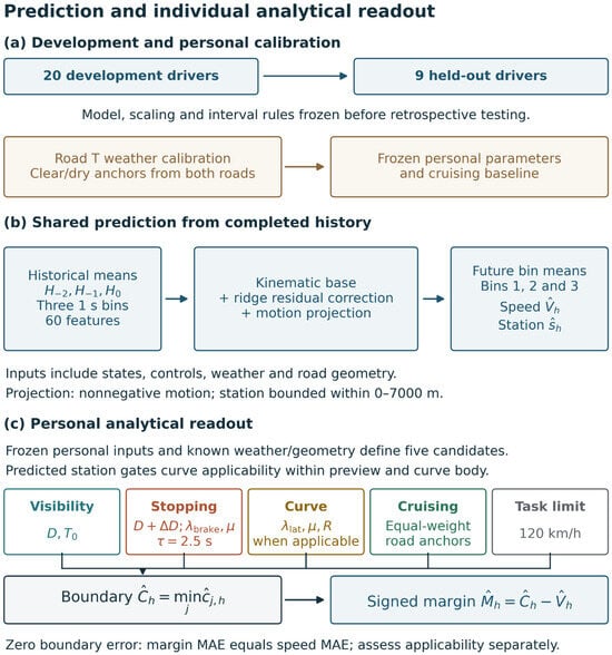
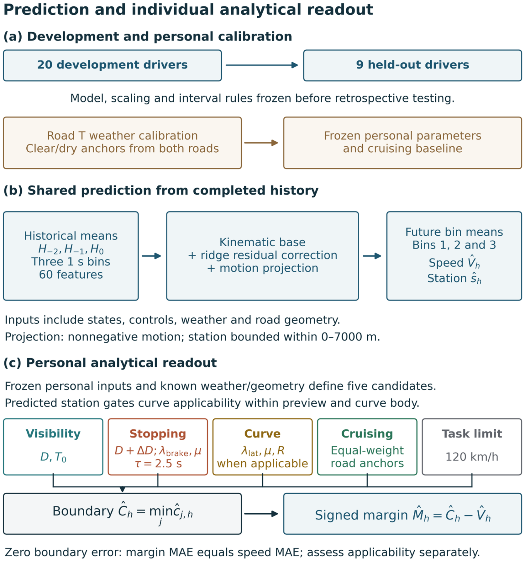
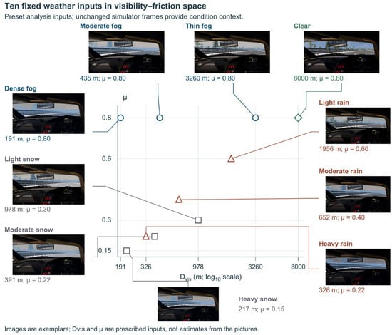
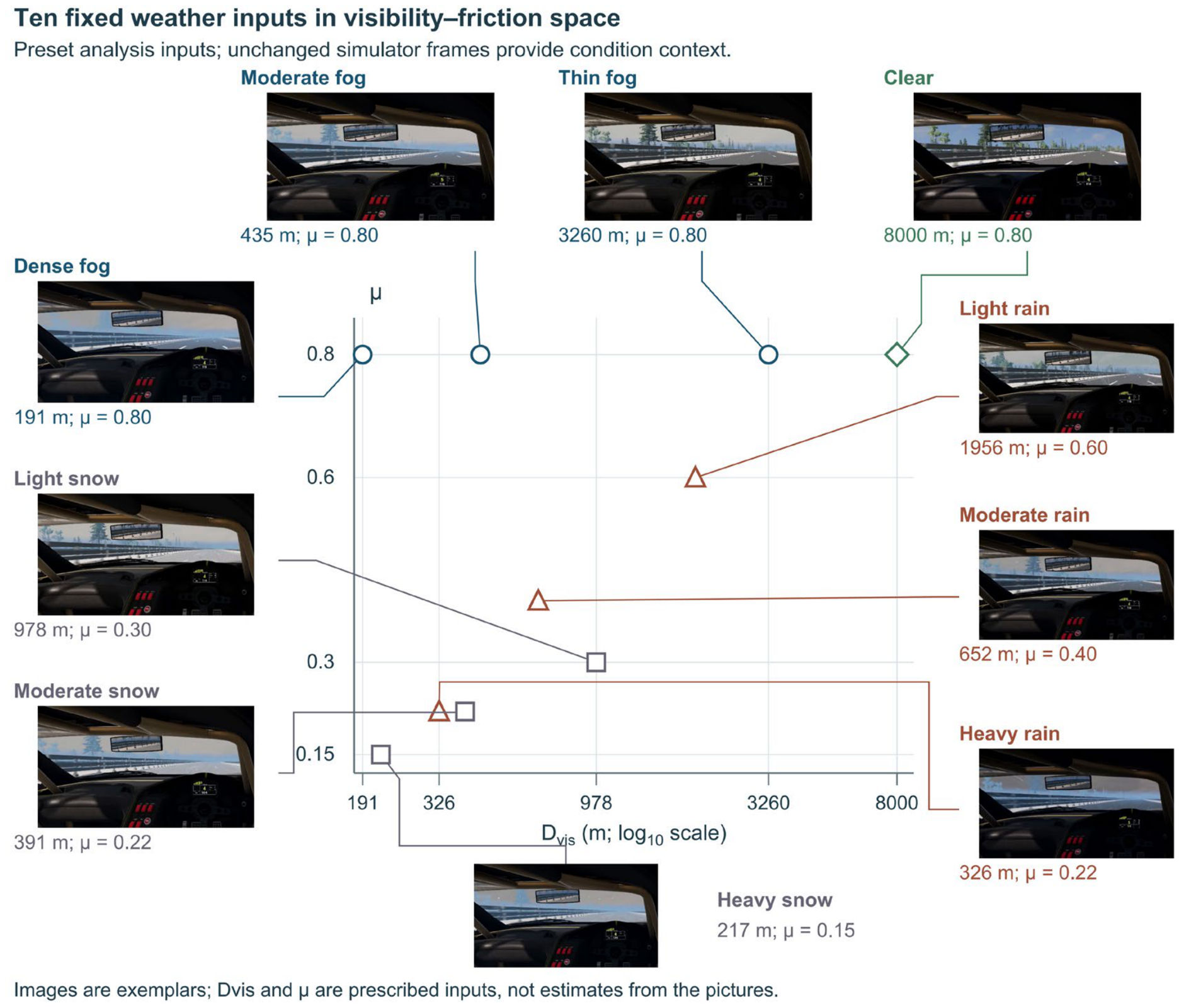
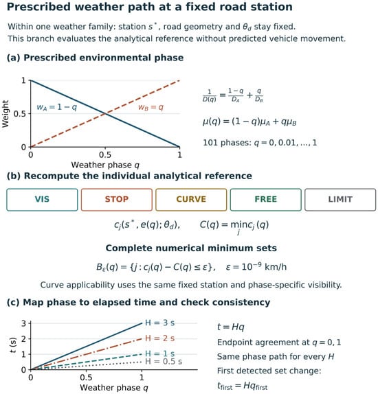
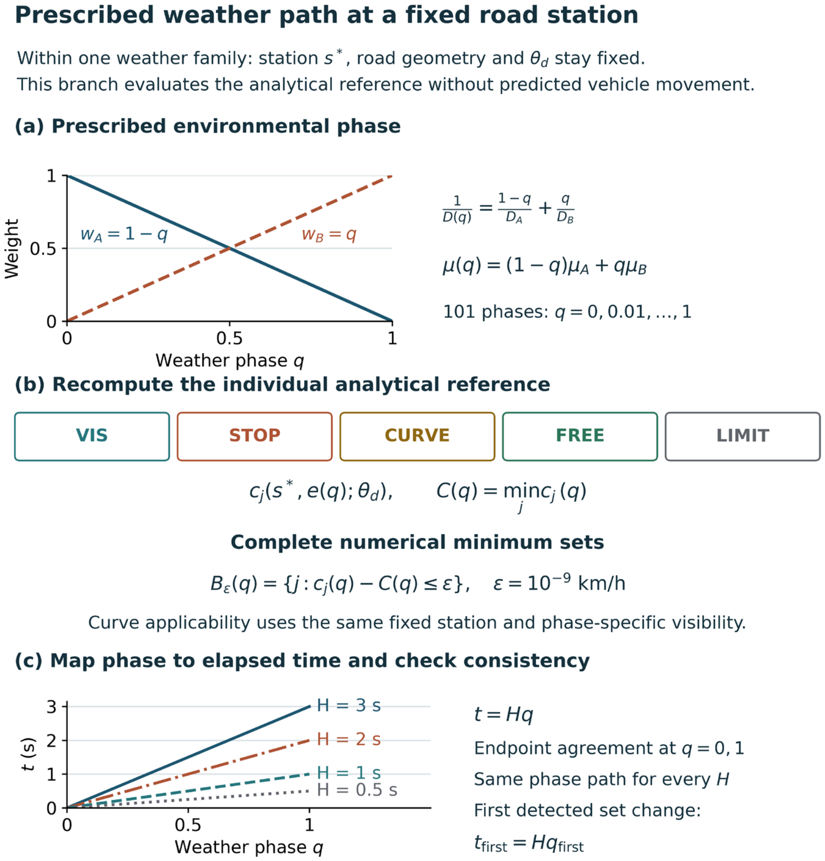
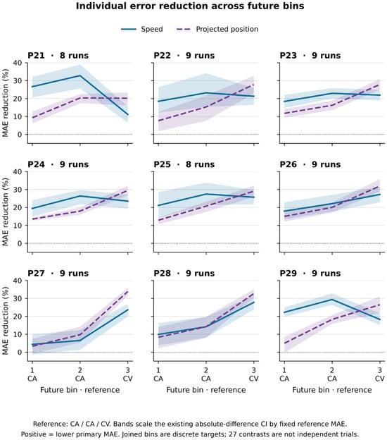
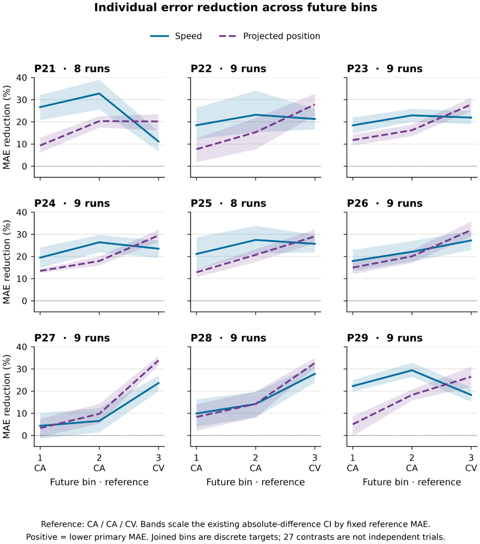
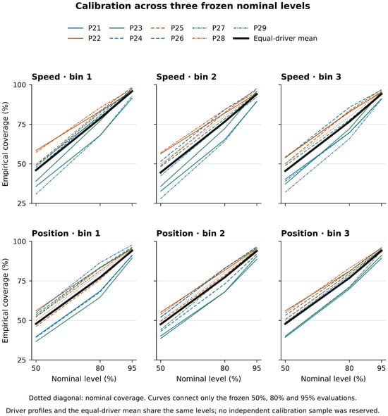
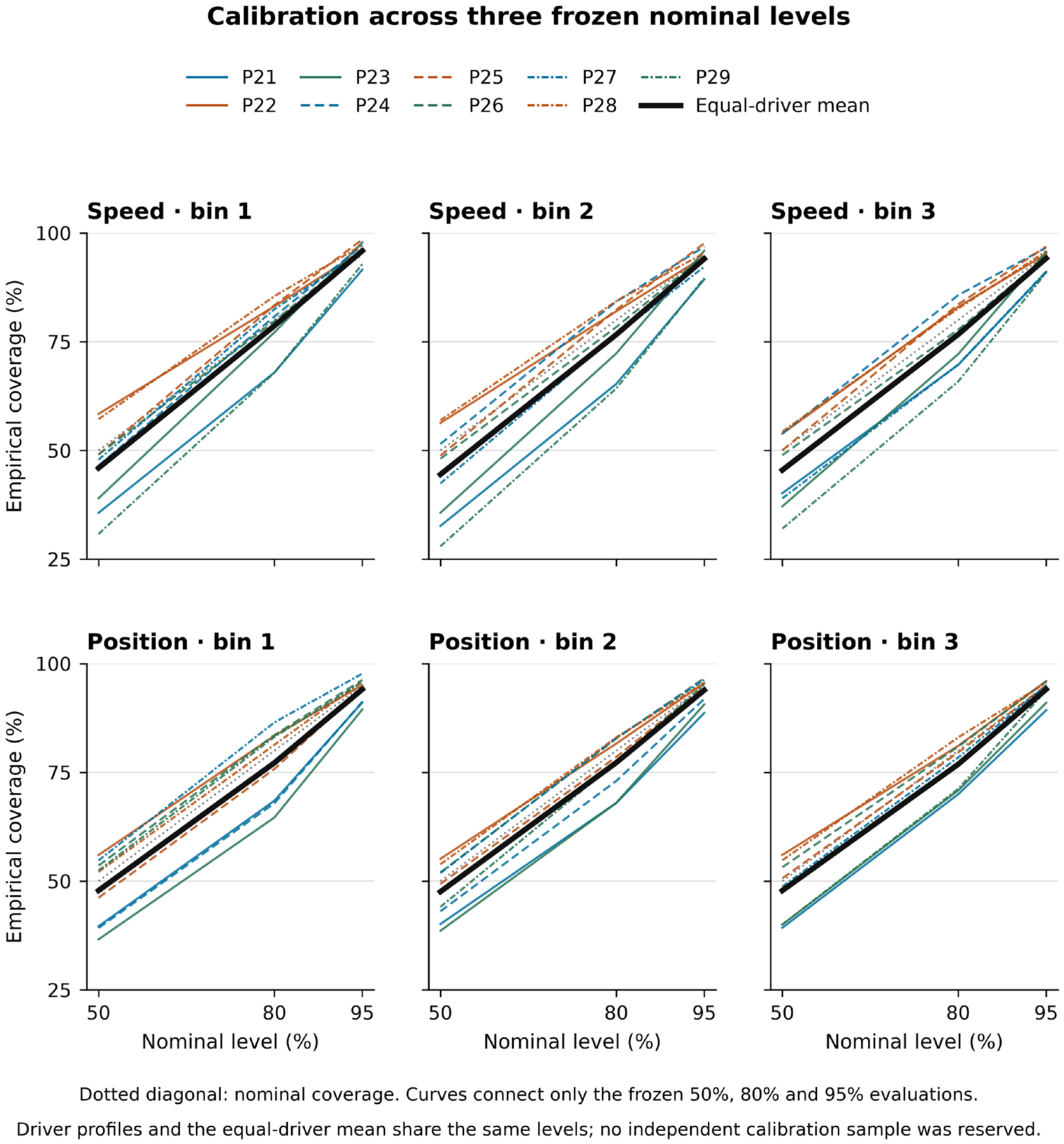
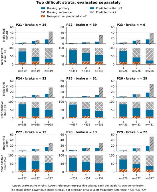
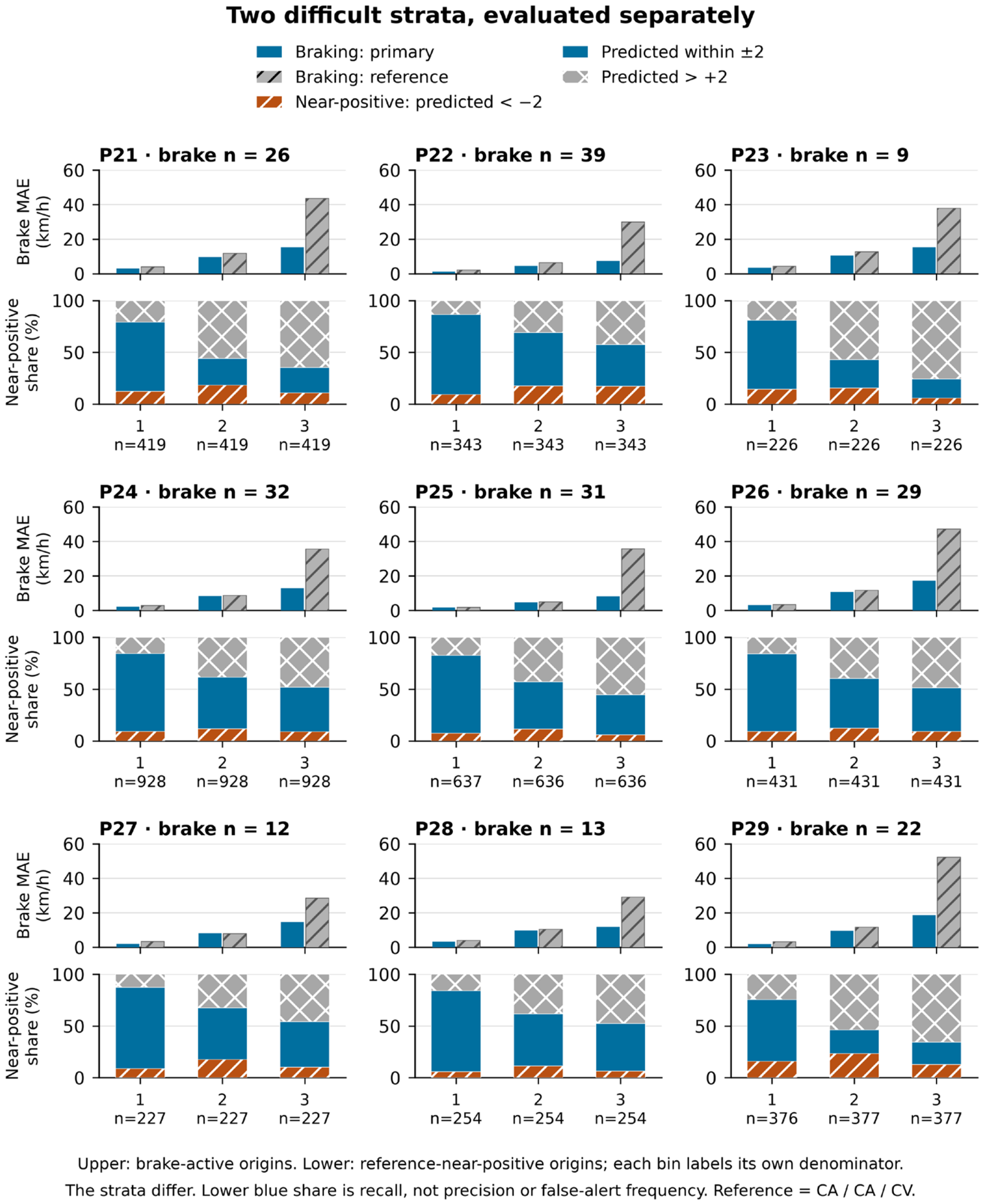
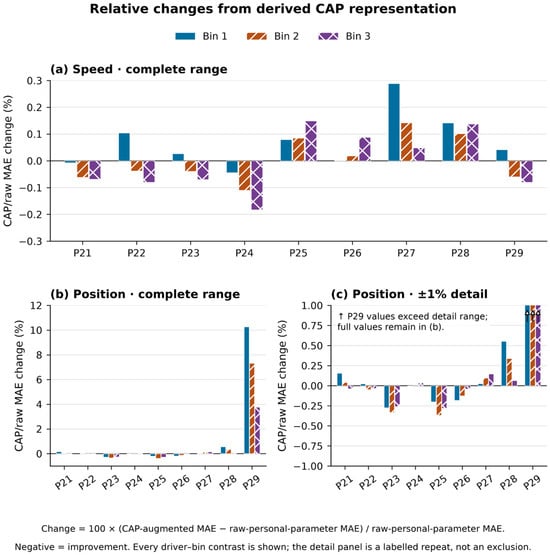
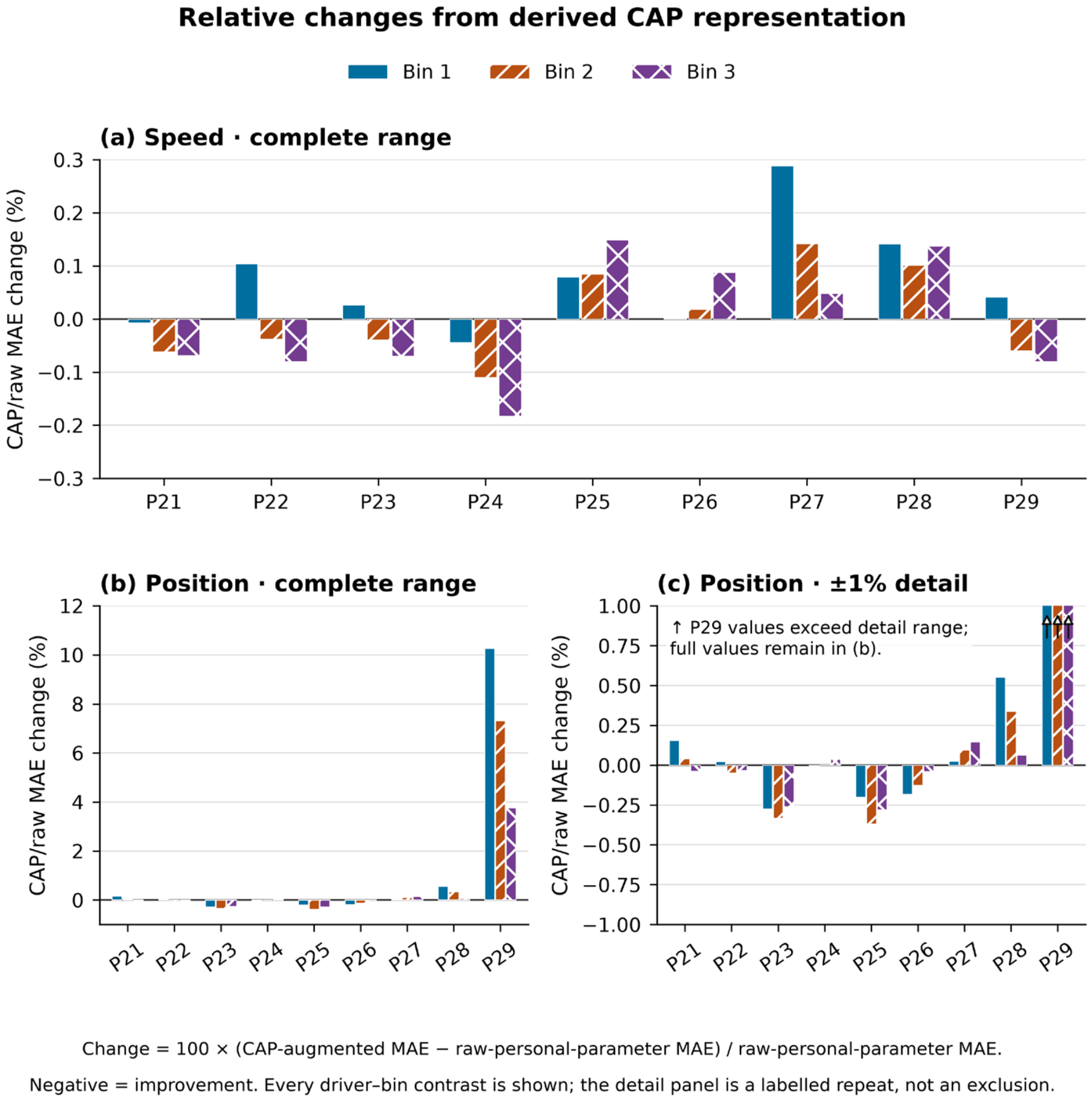
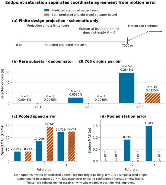
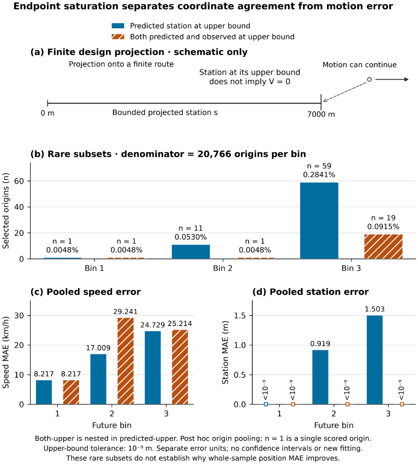
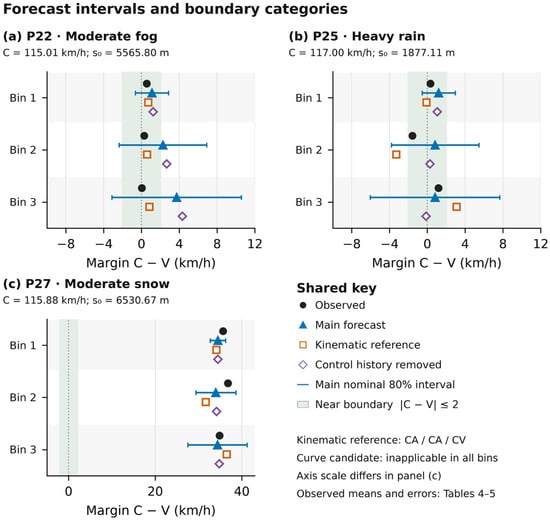
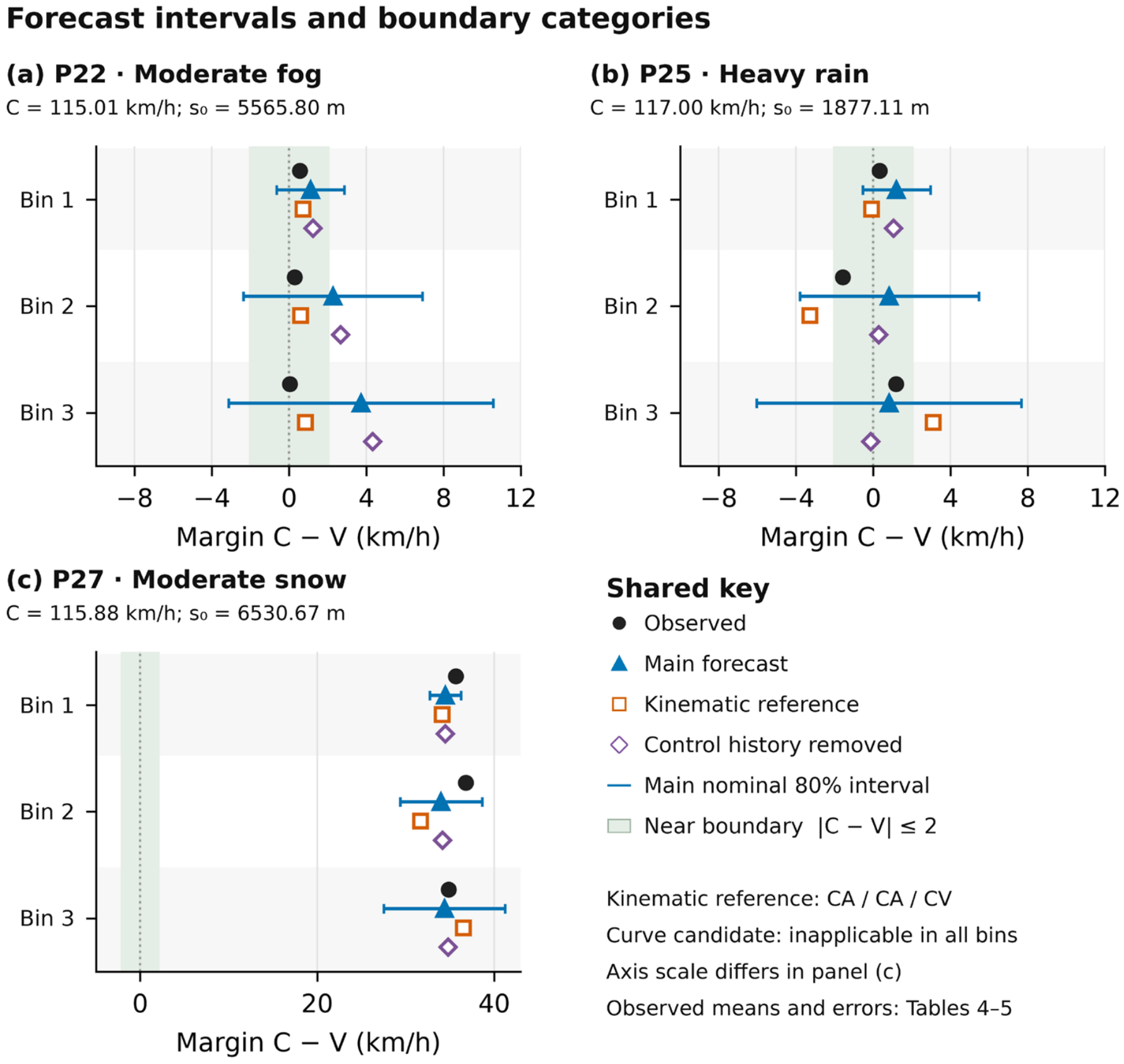
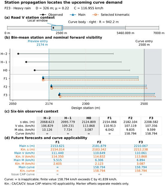
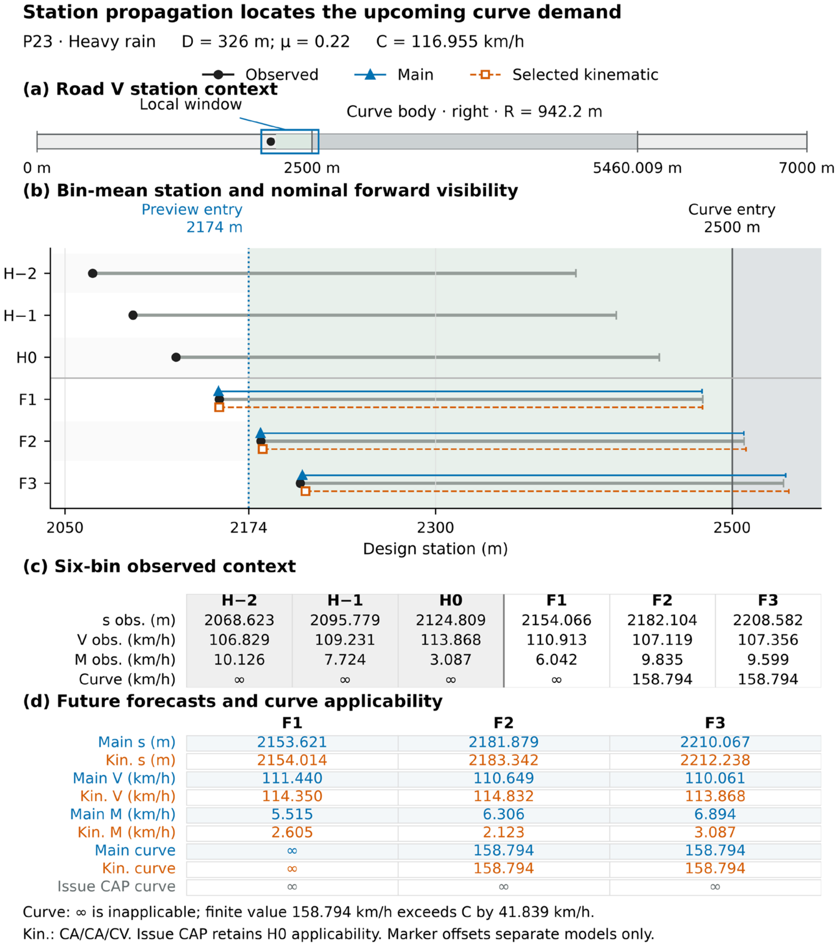
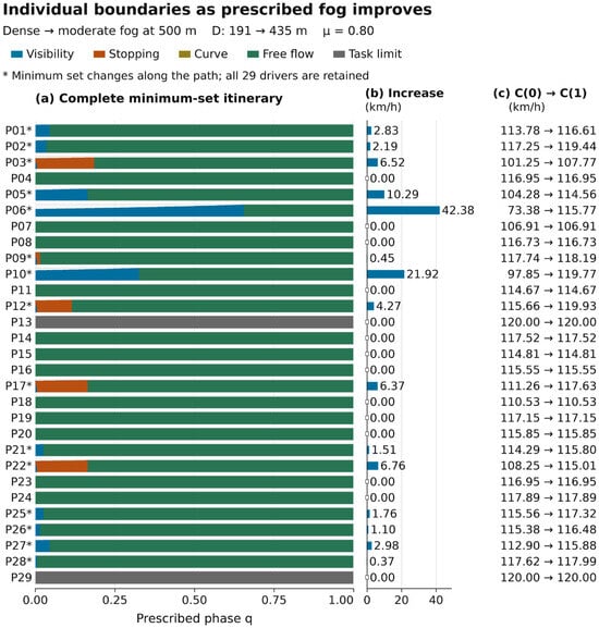
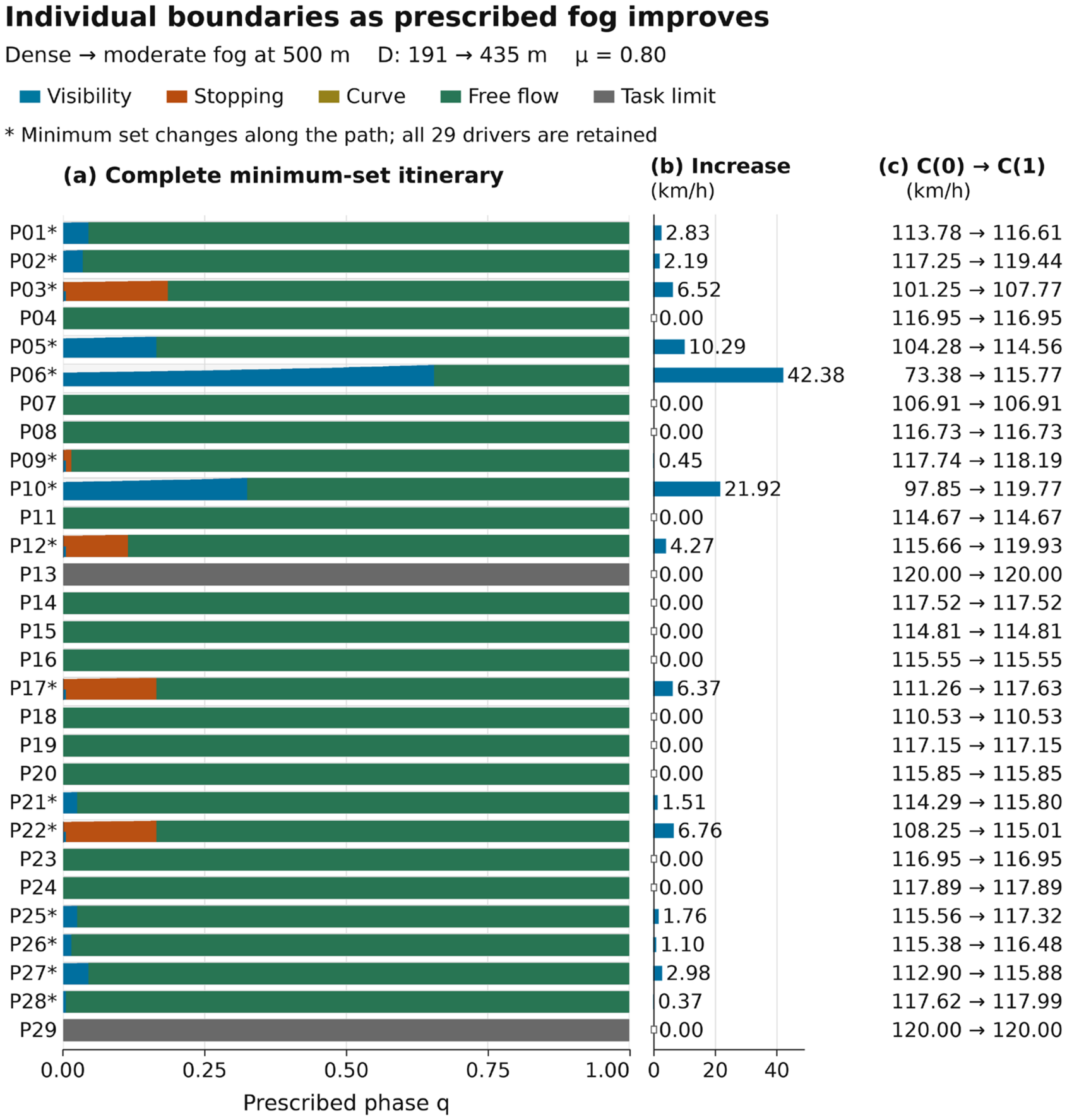

Disclaimer/Publisher’s Note: The statements, opinions and data contained in all publications are solely those of the individual author(s) and contributor(s) and not of MDPI and/or the editor(s). MDPI and/or the editor(s) disclaim responsibility for any injury to people or property resulting from any ideas, methods, instructions or products referred to in the content. |
© 2026 by the authors. Licensee MDPI, Basel, Switzerland. This article is an open access article distributed under the terms and conditions of the Creative Commons Attribution (CC BY) license.