


Abstract
The main challenge in railway predictive maintenance is balancing quantitative precision with interpretability, given the scarcity of experimental data linking dynamics and wear. In this study, a 1:20 scale test rig equipped with accelerometers, a gyroscope, and microscopy generated a multimodal dataset comprising 2460 cycles, synchronizing vibration data (1 kHz) with sequential images of the rolling surface. Two models were developed and compared: (1) Principal Component Analysis and Support Vector Machines (PCA+SVM) to classify four wear states, and (2) a Fully Connected Neural Network (FCNN) for Remaining Useful Life (RUL) regression. The PCA+SVM model achieved 84% accuracy and, through factor loadings, identified high-frequency energy (200–500 Hz) and kurtosis as physical precursors to fatigue. The FCNN model yielded a Mean Absolute Error (MAE) of 100 cycles (NMAE = 4.06%). Together, these results show that PCA+SVM is well-suited for interpretable diagnostics, while FCNN excels at quantitative forecasting, laying the groundwork for a hybrid predictive system.
1. Introduction
The rail transport sector is experiencing a global renaissance. Its energy efficiency, low carbon footprint, and capacity to move large volumes of passengers and freight make it a key component of future sustainable mobility [1]. The rail sector has grown steadily in recent decades, with significant investments in infrastructure and fleet modernization worldwide [2]. In Mexico, this momentum has materialized in the National Rail Plan, which includes the construction and rehabilitation of more than 3500 km of track for passenger trains, with flagship projects such as the Maya Train, the Interoceanic Train, and the Mexico City-Querétaro Train, the latter with speeds of up to 200 km/h [3].
However, this growth brings an unavoidable challenge: safety. Railway accidents, often linked to failures in critical components such as wheels and bogies, have devastating consequences in terms of loss of life, material damage, and environmental pollution. According to the International Union of Railways, 15% to 25% of railway accidents globally involve failures in these components, which are responsible for the vehicle’s dynamic stability and require continuous monitoring because of their constant exposure to mechanical loads and wear [4]. In Mexico, the situation is particularly worrying: between 2020 and 2025, more than 7000 railway accidents were recorded, including derailments, collisions, and pedestrian fatalities, resulting in 372 deaths and 837 injuries [5]. Recent tragedies, such as the derailment of the Interoceanic Train in Oaxaca in December 2025 that caused 14 deaths and 98 injuries, underline the urgency of implementing more effective and proactive monitoring systems [6].
Traditionally, railway wheel inspection relies on methods that require removing the vehicle from service, such as visual inspection, non-destructive testing (ultrasound, penetrant testing), or physical removal of the wheel for laboratory analysis. These processes are slow, expensive, and highly dependent on operator subjectivity: they can take up to 3 h per wheel and offer limited ability to detect early-stage failures under dynamic conditions [7,8,9]. Although static sensors exist for on-site monitoring, their ability to operate in real time without disrupting service remains limited [7]. This reality highlights the need for innovative approaches that enable continuous, non-invasive diagnostics.
In recent years, artificial intelligence has emerged as a powerful tool for condition monitoring and predictive maintenance in mechanical systems. Classical techniques such as Principal Component Analysis (PCA) and Support Vector Machines (SVM) have been widely used to classify failure states and reduce the dimensionality of complex signals [10,11]. PCA, in particular, not only reduces dimensionality but also allows analysis of loadings (weights of each component), providing valuable physical interpretability [12]. On the other hand, Convolutional Neural Networks (CNNs) have demonstrated great potential for extracting complex patterns from vibration signals and estimating the remaining useful life (RUL) of mechanical components [13]. Hybrid models such as MLP-RF (Multilayer Perceptron + Random Forest) have achieved up to 99% accuracy in correlating vibrations with defects in simulated data [14], while SVMs, despite their high accuracy (98.7%), have shown limitations in terms of the need for internal sensors that are unfeasible in urban operations [15].
However, significant gaps remain that limit the applicability of these approaches in real-world industrial settings. First, most models are trained on simulated or synthetic data, which limits their ability to generalize to actual operating conditions [16,17]. Second, publicly available data linking dynamic signals to actual physical wear are scarce; only 12% of studies in the literature share their complete databases [18]. Third, the preprocessing required by many models, especially those that convert 1D signals into 2D images to feed CNNs, adds unnecessary computational load and hinders implementation on embedded systems [19]. Finally, an open question remains in the scientific community: which type of model best suits each operational need? Is a model that classifies wear status into discrete categories better, or one that estimates a continuous value of remaining service life?
Recent literature (2022–2026) highlights a clear architectural dichotomy addressing these operational constraints. On one hand, classical hybrid pipelines such as PCA+SVM remain highly competitive for discrete fault diagnosis in rotating machinery and railway components (such as axle-boxes and bogies) [20,21]. Recent comparative studies confirm that PCA+SVM excels in scenarios with small sample sizes and strict memory constraints for edge-embedded deployment, where physical interpretability is required [22,23]. On the other hand, while deep convolutional architectures dominate RUL prognosis, recent frameworks emphasize the efficiency of Fully Connected Neural Networks (FCNNs) acting as multimodal fusers and continuous regressors [24,25]. FCNNs map 1D dynamic and visual features directly into life-cycle estimations, achieving high predictive accuracy without the prohibitive computational overhead of transforming time-series signals into 2D matrices [26].
To address these gaps, this paper presents a comparative study of two artificial intelligence approaches applied to a single experimental dataset. The dataset was generated on a 1:20 scale test bench replicating the wheel-rail interface. Its primary purpose is to reproduce the fundamental contact mechanics mechanisms (namely wheel-rail longitudinal creepage, localized surface microcracking, and contact fatigue) under strictly monitored, repeatable conditions to benchmark diagnostic and prognostic machine learning models. The vehicle was instrumented with accelerometers, a gyroscope, and digital microscopy to synchronously capture vibration signals (1 kHz) and sequential images of the wheel tread surface. Based on this dataset, two models were implemented and compared: (1) a PCA- and SVM-based classifier to categorize four wear states (new wheel, 820, 1640, and 2460 wear cycles), and (2) a FCNN for continuous regression of RUL.
PCA+SVM model was chosen for discrete diagnosis due to its low computational footprint on embedded microcontrollers, robustness against overfitting in moderate datasets, and physical interpretability via factor loadings. Conversely, the FCNN network was implemented for continuous RUL regression, enabling multimodal nonlinear mapping (vibrations and visual wear) without the high computational complexity of 2D convolutional networks.
The remainder of the article is structured as follows Section 2 details the experimental test bench, the wear protocol, the signal acquisition and processing pipelines, and the formulation of both machine learning architectures (PCA+SVM and FCNN). Section 3 presents the experimental results, encompassing vision-based wear quantification, dynamic correlation analyses, and the diagnostic and prognostic validation of both models. Section 4 discusses these findings, evaluating model performance, physical interpretability, and the transferability of scaled dynamic parameters to full-scale rolling stock. Finally, Section 5 summarizes the primary conclusions and outlines avenues for future research.
2. Materials and Methods
2.1. Test Bench and Wear Protocol
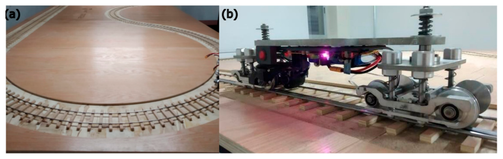
A 1:20 scale railway test bench (Figure 1) was employed to replicate the wheel-rail interface under laboratory conditions (Figure 1a). The track is a closed circuit with a β-shaped geometry, 5.38 m long and 2.02 m wide, with straight sections and tight curves to evaluate different operating regimes.
Figure 1.
Test bench: (a) Panoramic view of the track, (b) Railway vehicle.
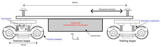
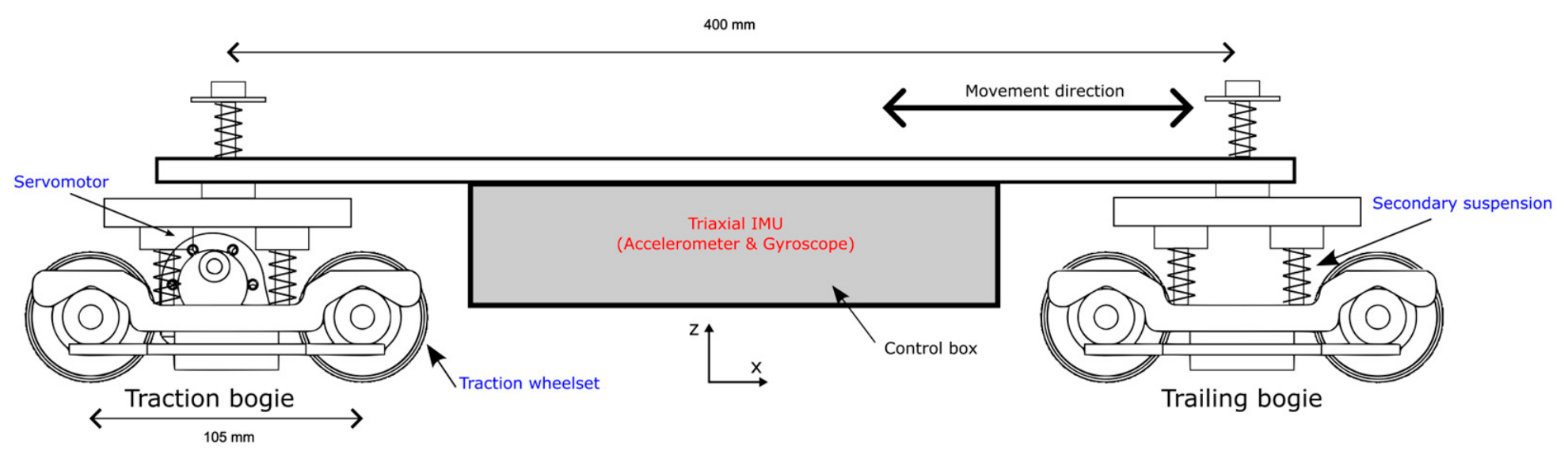
The scaled railway vehicle consists of a single wagon mounted on two bogies (Figure 1b). Figure 2 details the vehicle’s schematic layout, main dimensions, and instrumentation. The vehicle has a total mass of 4.28 kg, resulting in an evenly distributed static normal load of approximately per wheel ( across the 8 wheels). The chassis incorporates a secondary suspension with coil springs () and a wheelbase of 105 mm per bogie, with a distance between bogie centers of 400 mm. Traction is provided by a servomotor coupled exclusively to the rear bogie (traction bogie), leaving the front bogie unpowered (trailing bogie). This configuration isolates wheel slip during traction and braking maneuvers on the driven wheelset. Dynamic motion was monitored using a commercial 6-degree-of-freedom (6-DoF) Inertial Measurement Unit (IMU, model LSM6DS3, STMicroelectronics, Geneva, Switzerland) rigidly mounted inside the central control box near the vehicle’s center of gravity, as depicted in the schematic diagram of Figure 2. The sensor integrates a 3-axis digital accelerometer and a 3-axis digital gyroscope in a single package. For the experimental campaign, the accelerometer was configured to a full-scale range of ±4 g (sensitivity of 0.122 mg/LSB), while the gyroscope was configured to an angular rate range of ±125 °/s with an operational span of ±143 °/s (sensitivity of 4.375 m°/s/LSB).
Figure 2.
Schematic diagram of the 1:20 scale railway vehicle showing main geometric dimensions (wheelbase: 105 mm, bogie spacing: 400 mm), secondary suspension, center of gravity, IMU location, and drive system configuration (traction bogie vs. trailing bogie).
The 1:20 scaled vehicle was dimensionally synthesized based on the geometric and topological proportions of a standard four-axle regional passenger carbody mounted on two two-axle bogies. Applying the geometric scaling factor ( 1:20), the nominal wheel diameter of 45 mm corresponds to a full-scale wheel diameter of 900 mm, which aligns with standard UIC nominal wheel dimensions (typically 840–920 mm). Similarly, the 105 mm bogie wheelbase and 400 mm bogie pivot spacing scale to 2.10 m and 8.00 m, respectively, representing typical dimensions for compact passenger and metro bogies. Under volumetric mass scaling (), the vehicle mass of 4.28 kg corresponds to a prototype tare mass of approximately 34.24 tonnes (), yielding an equivalent static wheel load of 42.0 kN per wheel. While geometric scaling was strictly maintained, complete dynamic similarity (Froude and Cauchy numbers) was relaxed to prioritize controlled contact wear in the laboratory, as addressed in the discussion.
While this 1:20 scale does not reproduce Froude’s dynamic similarity in absolute magnitude, it facilitates the generation of a large, controlled dataset under repeatable laboratory conditions, serving as a testbed for algorithm comparison. Quantitative extrapolation to real-world scale is addressed in the discussion.
To induce controlled wear, an accelerated life testing protocol specifically designed for this evaluation was implemented. Wear is induced through repeated acceleration and braking cycles on the straight portion of the track, where wheel-rail slippage removes material from the track surface. During braking, the drive wheel continues to rotate due to inertia as the vehicle decelerates, generating controlled slippage that results in material loss.
2.2. Calculation of Wheel Wear
The wear levels (820, 1640, and 2460 wear cycles) were defined from the Archard model [27], which quantifies the volume of material removed during sliding contact:
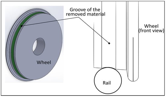
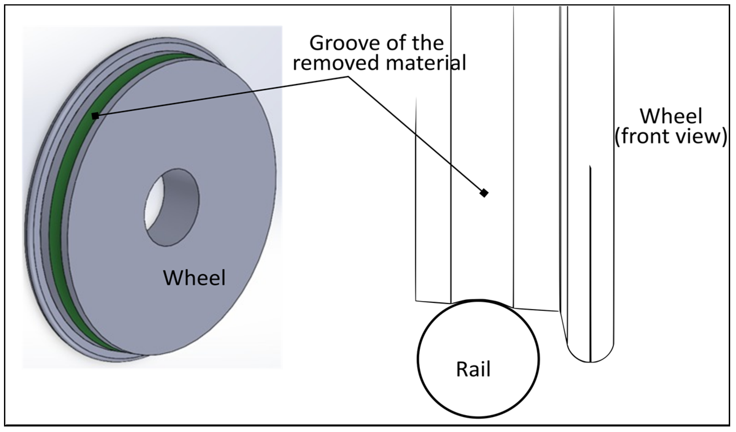
where is the volume of material removed, is the wear coefficient (which varies with sliding speed and contact pressure), is the sliding distance, is the normal load between the wheel and the rail, and is the hardness of the softest material (aluminum 7075-T6, 345 MPa). Figure 3 shows the schematic representation of the volume of material removed in the form of an annular groove.
Figure 3.
Schematic representation of wear on the wheel. The removed volume forms an annular groove with an outer radius of 22.5 mm and a depth of 0.13 mm, similar to the radius of the rail.
It is important to emphasize that Archard’s wear formulation was implemented as an analytical planning framework to estimate the degradation progression rate and define the discrete testing milestones (820, 1640, and 2460 cycles), rather than as a direct substitute for physical metrology. Because the estimated terminal volumetric loss (20 mm3) and its corresponding cumulative groove depth (0.13 mm) represent theoretical estimations based on nominal contact parameters at the final stage, the actual physical progression of damage was experimentally tracked and validated via sequential digital microscopy. It is important to clarify that in the railway wheel-rail interface, pure monotonic volumetric wear (continuous material removal) and Rolling Contact Fatigue (RCF, characterized by stochastic surface micro-spalling) are distinct but coexisting phenomena. While this work uses the term ‘wear’ in a broad operational context to describe overall wheel tread degradation, the 2D optical metric () does not directly measure monotonic volumetric loss. Instead, quantifies the extent of visible surface distress (pitting, microcracks, and spalling), following established tribological vision-based damage quantification methodologies [28,29,30]. This empirical surface damage ratio provided the direct experimental ground truth used to train and evaluate the machine learning models. Using as an operational proxy is justified because the progression of RCF and the resulting surface roughness are the primary exciters of the dynamic vibration signatures being monitored.
The wear coefficient was determined based on the contact pressure (calculated using Hertz theory [31]) and the sliding velocity. Table 1 summarizes the model parameters.
Table 1.
Archard model parameters [27] and Hertz results.
Based on these parameters, Archard’s formulation was used to define the target operational horizon (), which corresponds to an estimated cumulative volumetric loss of 20 mm3 (equivalent to an idealized annular groove depth of 0.13 mm). To establish discrete degradation milestones across the life cycle, the experimental thresholds were set at equal operational increments: low wear at 820 cycles (theoretically yielding a cumulative loss of ≈6.67 mm3 and a depth of 0.043 mm), medium wear at 1640 cycles (≈13.33 mm3 and 0.087 mm), and severe wear at 2460 cycles (20 mm3 and 0.13 mm). These values served as analytical reference benchmarks to schedule inspection intervals rather than direct measures of real-time surface degradation.
2.3. Design of Experiments
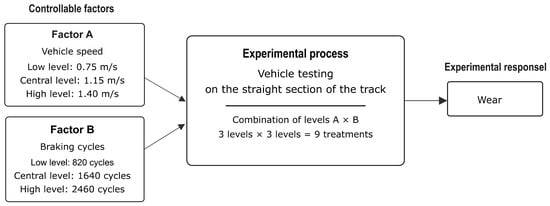
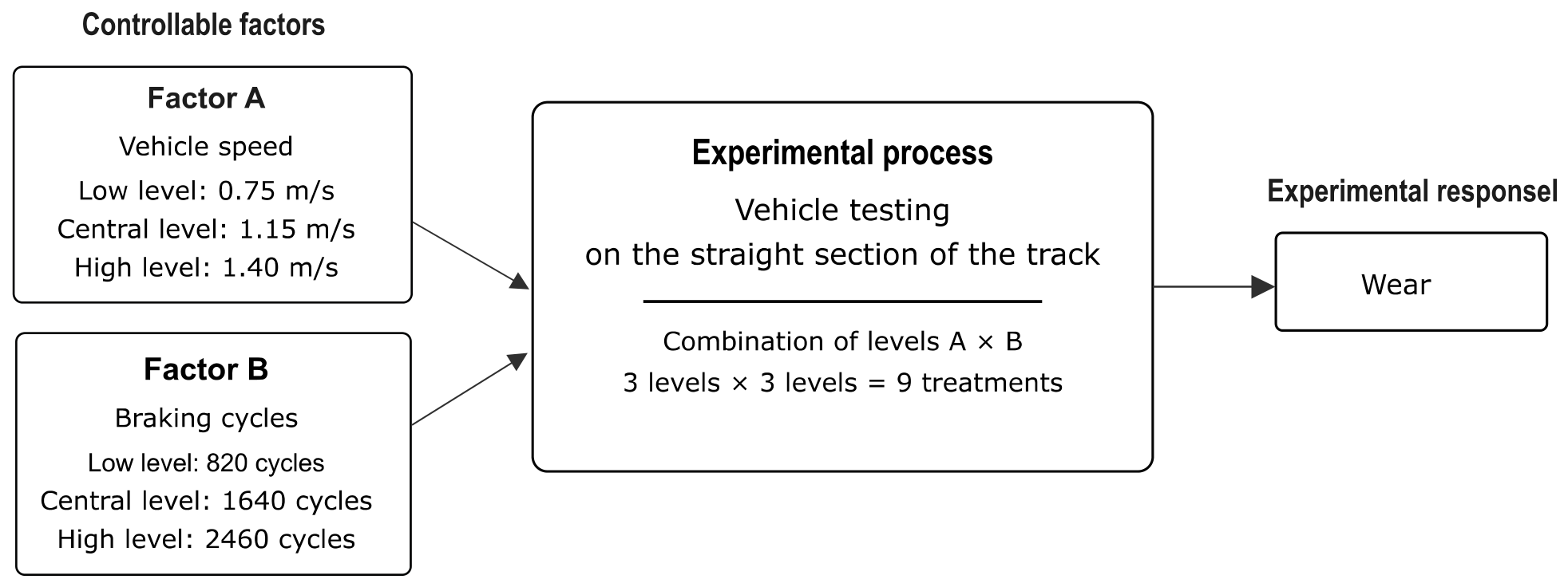
A full factorial experimental design based on Archard wear formulation was implemented to validate theoretical predictions and synthesize a comprehensive dataset encompassing diverse wear states. The experimental design considered two variables of interest: vehicle speed and the number of braking cycles. Speed was established at three levels: low (0.75 m/s), medium (1.15 m/s), and high (1.4 m/s). The number of braking cycles was also defined at three levels, corresponding to the wear states estimated from Archard’s model: 820 cycles (low), 1640 cycles (medium), and 2460 cycles (high). All wear tests were performed on the straight section of the track, where controlled slippage is induced during braking. Figure 4 presents the experimental design diagram. The evaluated response variable was the surface damage ratio , defined as the percentage of defect pixels (pitting, microcracks, and detachment) relative to the total area of the evaluated Region of Interest (ROI):
where represents the segmented damage pixels in the binary mask and is the total pixel count within the fixed bounding box. This scalar metric serves as an empirical 2D proxy for progressive contact distress rather than absolute volumetric wear.
Figure 4.
Schematic of the experimental design 3k. Factor A: vehicle speed (0.75, 1.15 and 1.4 m/s). Factor B: braking cycles (820, 1640 and 2460 cycles).
The objective of the experimental design was not to perform an analysis of variance (ANOVA) to quantify the statistical significance of the factors (speed and cycles), but to generate a labeled, balanced dataset covering the full spectrum of wheel degradation. Consequently, despite the absence of experimental replicates, each factorial combination was evaluated singularly to prioritize the breadth of dynamic conditions (across three speed levels) over statistical repeatability. This approach aligns with benchmark studies in machine learning-based lifespan forecasting [10], where dataset richness takes precedence over classical statistical design.
Wear was assessed after complete blocks of 19 cycles by capturing microscopic images of the wheel surface before and after each block, until the wear levels defined in the model were reached. For each distinct degradation state (initial, intermediate, and final), a total of 60 high-resolution images of the wheel tread surface were acquired, yielding 240 images across the entire experiment. Simultaneously, vibration signals were recorded at 1 kHz and temporally synchronized with the wear stages. This allowed for a direct correlation between the evolution of surface damage (response variable) and the vehicle’s dynamic signatures (predictor variables). The experiments were conducted under controlled environmental conditions (22 ± 2 °C).
Surface wear was quantified within a fixed ROI centered on the contact track (). Images were converted to grayscale and initially smoothed with a 5 × 5 Gaussian filter to reduce high-frequency sensor noise. Rather than using a simple global brightness cutoff, which is highly susceptible to uneven illumination and reflections, the segmentation was performed by combining adaptive thresholding (to account for localized lighting variations) and Canny edge detection (with hysteresis thresholds of 50/150 to identify the high spatial frequency gradients characteristic of microcracks and pit boundaries) via a bitwise-OR operation [32,33]. To ensure that the resulting binary mask isolated genuine surface damage rather than capturing random optical white noise, morphological opening and closing operations with a 3 × 3 kernel were applied [32]. These morphological filters specifically eliminated isolated 1- or 2-pixel anomalous artifacts and consolidated adjacent defect structures. Finally, the damage ratio was computed as the percentage of validated defect pixels relative to the total ROI area.
2.4. Vibration Signal Processing
Dynamic acceleration and rotational velocity signals were acquired from the on-board LSM6DS3 IMU at a sampling rate of 1 kHz. Signal conditioning and anti-aliasing were handled directly in hardware: the IMU integrates an embedded analog low-pass filter prior to the analog-to-digital converter (ADC), followed by an internal digital low-pass filter (LPF) that bounds the effective operational bandwidth to the Nyquist cut-off ( Hz). No secondary software-based digital smoothing or band-pass filtering was applied to the raw signals, ensuring that high-frequency transient shocks and impulsive characteristics (such as kurtosis and crest factor in the 200–500 Hz range) induced by surface micro-pitting were fully preserved. Recordings were acquired during braking intervals on the straight track section, segmenting the continuous time series into discrete windows of samples (1 s duration) to isolate the wheel-rail dynamic interaction under controlled slippage.
To feed the different predictive schemes, two independent feature extraction strategies were designed in the time and frequency domains:
2.4.1. Multichannel Extraction for Classification (PCA+SVM)
The 6 kinematic channels of the IMU (accelerations and angular velocities) were processed simultaneously. For each channel, the following time-domain statistical descriptors were calculated: arithmetic mean, standard deviation, root mean square (RMS), peak-to-peak amplitude, kurtosis, skewness, and crest factor:
In the frequency domain, using the Fast Fourier Transform (FFT), the power spectrum was divided into three key spectral bands: low frequency (0–100 Hz, associated with rigid body and suspension dynamics), mid frequency (100–200 Hz, representative of bogie and yaw vibrations), and high frequency (200–500 Hz, sensitive to fine roughness and surface micro-impacts). Integrating these metrics produced an overall vector of 60 features per time window.
2.4.2. Single-Channel Extraction and Multimodal Fusion for Regression (FCNN)
For continuous wear forecasting, the longitudinal acceleration component was evaluated to capture dynamic signatures along the primary direction of motion. A total of 22 dynamic features were extracted per time window:
- 12 time-domain statistical parameters: arithmetic mean, standard deviation, root mean square (RMS), maximum peak value, minimum peak value, peak-to-peak amplitude, kurtosis, skewness, crest factor, dynamic range, signal temporal energy, and square root of the mean amplitude.
- 10 frequency-domain (spectral) descriptors: calculated via the Fast Fourier Transform (FFT), comprising seven sub-band spectral energies (0–50 Hz, 50–100 Hz, 100–150 Hz, 150–200 Hz, 200–300 Hz, 300–400 Hz, and 400–500 Hz), the spectral centroid, the dominant harmonic peak amplitude, and the total FFT spectral energy.
This vector of 22 dynamic variables was merged with the percentage of worn area () derived from microscopic image processing, forming a multimodal input vector of 23 features normalized using Z-score standardization:
where represents the original feature, the sample mean, and the standard deviation.
2.5. Machine Learning Models
The baseline experimental dataset (comprising 240 synchronized dynamic windows) was randomly partitioned using a Pareto-based 80/20 ratio, allocating 80% (192 samples) to the training set and strictly reserving 20% (48 samples) as an independent test set for unbiased model evaluation. Subsequently, as detailed in Section 3.4, data augmentation was applied to the vibration signals to expand the training set to 1920-time windows.
All data processing, computer vision routines, and predictive algorithms were developed in Python (v3.10.12). Classical machine learning pipelines, including PCA projection, SVM classification, cross-validation, and scaling, were implemented using scikit-learn (v1.4.2). The FCNN regression architecture and training callbacks were constructed using TensorFlow (v2.16.1) with Keras. Image processing for surface wear quantification was executed using OpenCV (v4.9.0), while spectral FFT decompositions and scientific calculations utilized scipy (v1.12.0) and numpy (v1.26.4).
2.5.1. Fully Connected Neural Network (FCNN)
To enable quantitative wear forecasting, a sequential Fully Connected Neural Network (FCNN) architecture [34] was developed to represent the complex, nonlinear relationship between dynamic vibration signatures, surface damage metrics, and remaining operational cycles.
The model architecture consists of the following components:
- The input layer receives the multimodal vector of 23 features (22 longitudinal vibration descriptors and the percentage of visual wear).
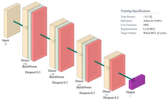
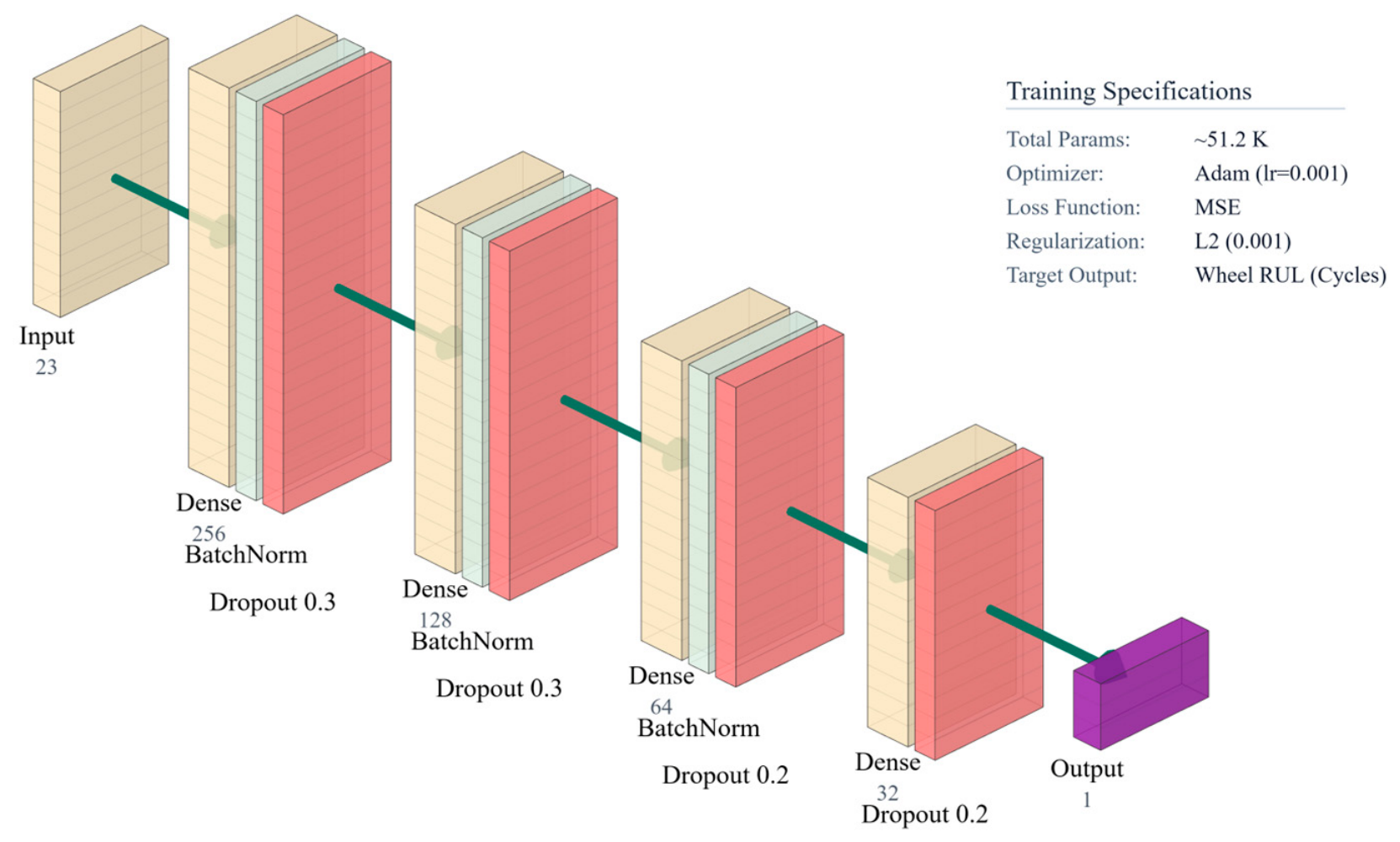
- The hidden layers follow a descending funnel topology comprising four sequential dense layers of 256, 128, 64, and 32 neurons, respectively, yielding approximately 51.2 k trainable parameters. This configuration was selected through an empirical grid search evaluating depth (2 to 5 hidden layers) and width to ensure smooth dimensional contraction from the 23-feature multimodal space into a single continuous RUL prediction without gradient saturation. Intermediate layers utilize the ReLU activation function paired with an weight regularization penalty (λ = 0.001) to penalize large synaptic weights. Additionally, each hidden layer incorporates Batch Normalization and Dropout (30% in the first two layers, 20% in the subsequent layers) to disrupt neuron co-adaptation and prevent overfitting on the baseline dataset.
- The output layer is a single neuron with linear activation that directly estimates the continuous value of the RUL in operating cycles. In this investigation, RUL is formally defined as the number of braking cycles remaining before the wheel reaches its terminal degradation state. This terminal threshold of 2460 cycles was not an arbitrary experimental failure, but rather a predefined operational boundary derived a priori from Archard’s formulation to reach the target allowable scaled wear depth of 0.13 mm. It was adopted as the absolute end-of-life limit for this experimental campaign because continuing the tests beyond this level of volumetric loss would result in severe geometric interference between the wheel flange and the rail, compromising the safe dynamic guidance of the scaled vehicle. Mathematically, for any given measurement window , the target RUL is computed using a linear cumulative degradation model:where cycles represents the end-of-life cycle threshold and is the cumulative number of completed braking cycles at that operational stage. This formulation allows the FCNN to map the complex multimodal feature space into a continuous operational life countdown.
The Adam optimizer trained the network by minimizing the Mean Squared Error (MSE) loss function. MSE is computationally preferred as the optimization objective during backpropagation because its derivative is continuous and proportional to the error magnitude, efficiently penalizing large prediction discrepancies to accelerate gradient descent:
where denotes the ground-truth remaining useful life in operating cycles, represents the network prediction, and is the mini-batch size (set to windows in this study) utilized during each training step. While MSE serves as the internal mathematical loss function, the Mean Absolute Error (MAE) was selected as the final external evaluation metric to report performance because it preserves the original linear physical units (cycles) without the quadratic outlier inflation inherent to MSE.
An initial learning rate of was established via grid search over , providing an optimal balance between stable gradient steps and convergence speed. To ensure stable convergence, two dynamic control mechanisms were implemented during training: an adaptive learning rate reducer (ReduceLROnPlateau) that halves the step size if the validation loss plateaus, and an early stopping mechanism (Early Stopping). In the context of deep learning, an epoch is defined as one complete forward and backward pass of the entire training dataset through the neural network. The early stopping mechanism was configured with a patience of 15 epochs, meaning training halts automatically if the validation loss does not improve for 15 consecutive passes, thereby ending the iteration at the point of optimal generalization and restoring the best network weights [34] (Figure 5).
Figure 5.
Architecture of the FCNN developed for RUL regression.
The model processes a multimodal input vector of 23 features through four dense hidden layers (256, 128, 64, and 32 neurons). Batch normalization and dropout mitigate overfitting, culminating in a single linear output neuron for quantitative estimation of the remaining cycles.
It is worth noting that the FCNN does not process high-dimensional 2D image matrices directly; rather, it takes a compact 1D vector of 23 numerical features (22 vibration descriptors and a single scalar damage ratio ). To ensure statistical robustness and prevent overfitting given the baseline sample size (240 synchronized windows), data augmentation was applied strictly to the training split (80%, 192 samples). Two specific signal engineering techniques were employed [35]: (1) time-shifting, which involves displacing the discrete vibration signal array along the time axis by a defined temporal lag ( samples) to simulate slight sensor triggering delays; and (2) Gaussian noise injection, which adds normally distributed random values to the signal to simulate environmental sensor noise, maintaining a controlled Signal-to-Noise Ratio (SNR) of 30 dB. These domain-specific augmentations expanded the training set to 1920 windows while preserving an uncorrupted, strictly independent test set (20%, 48 samples). Additionally, structural overfitting was strictly controlled via Batch Normalization, Dropout (20–30%), weight regularization ), and early stopping ( epochs).
2.5.2. Principal Component Analysis and Support Vector Machines (PCA+SVM)
To complement qualitative diagnostic techniques, a hybrid framework integrating Principal Component Analysis (PCA) [36] and Support Vector Machines (SVM) [37] was developed to balance computational efficiency with the physical interpretability of mechanical feature sets.
In the first stage, PCA was applied to the complete vector of 60 multichannel features () to project the information onto a lower-dimensional orthogonal subspace. This step not only eliminates redundancy and statistical noise, but also extracts the loadings of each principal component to identify which physical variables and spectral bands dominate wear variance.
Subsequently, the projected coordinates of the retained principal components were used as input variables for an SVM classifier to separate the four wear severity levels. To resolve nonlinear class overlap, a Support Vector Classifier (SVC) with a Radial Basis Function (RBF) kernel was trained. The optimal hyperparameters were determined via exhaustive grid search evaluated with 5-fold stratified cross-validation over the search space ( and ), yielding optimal values of and (Figure 6).
Figure 6.
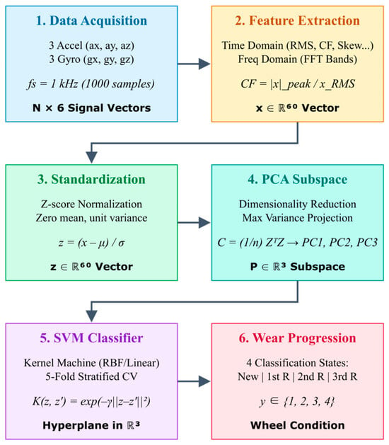
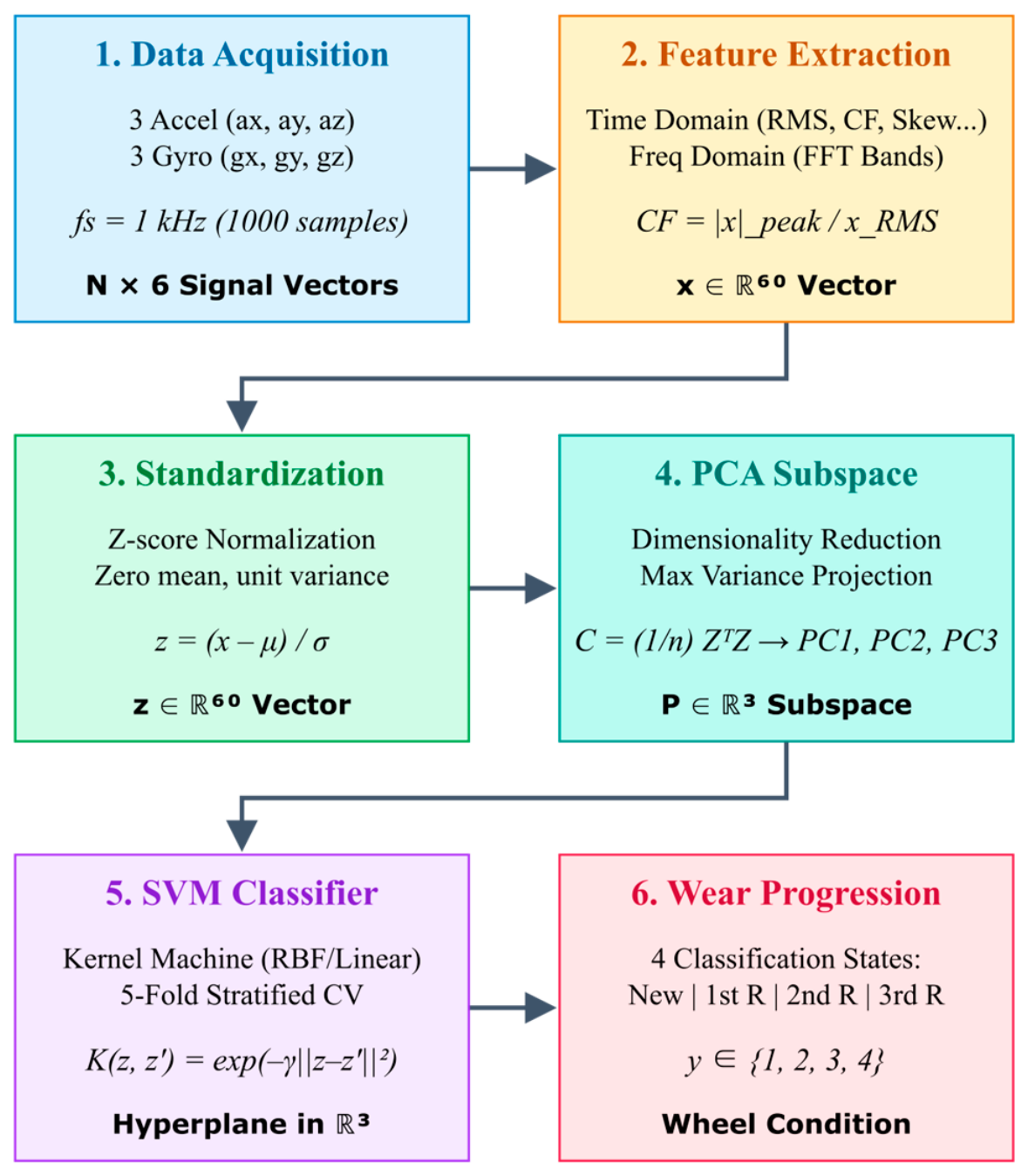
Flowchart of the PCA+SVM hybrid methodology for wheel diagnosis.
The sequential process involves multichannel acquisition of inertial signals, extraction of a vector of 60 dynamic features (temporal and frequency-based), and standardization using Z-scores. Next, PCA reduces dimensionality by projecting the data onto its principal components, enabling an SVM classifier to be trained to categorize degradation into four operating states.
3. Results
3.1. Quantification of Wear Using Image Processing
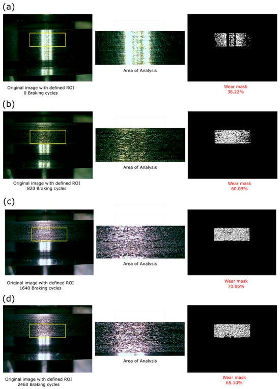
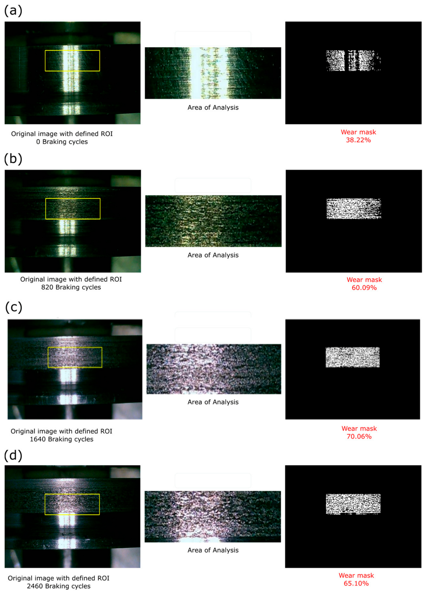
Machine vision methodology enabled quantification of the percentage of worn area across the four predefined degradation states. Figure 7 shows the segmentation and quantification process of surface wear for a new wheel (0 cycles), low level (820 cycles), medium level (1640 cycles), and high level (2460 cycles).
Figure 7.
Surface wear segmentation and quantification workflow across four operational stages: (a) Pristine wheel (0 braking cycles, baseline specular finish); (b) Low wear (820 braking cycles); (c) Medium wear (1640 braking cycles); and (d) High wear (2460 braking cycles). Each panel displays the original image with the fixed bounding ROI (left), the extracted contact area (middle), and the refined binary damage mask with the resulting surface damage ratio Aw % (right).
In the initial pristine state (0 cycles), the wheel surface retains a polished, highly specular finish. Consequently, the edge detection algorithm captures the high spatial gradients generated by inherent lathe machining grooves and localized lighting reflections, yielding a baseline optical edge density of 38.22% (Figure 7a). It is crucial to address how reflections and polishing are differentiated from genuine damaged pixels: this initial 38.22% baseline does not represent volumetric material loss, but rather the intrinsic specular response and surface roughness of the unoperated wheel. Therefore, is strictly utilized as a relative operational metric. Genuine progressive contact damage (pitting, microcracks, and spalling) is reliably differentiated and quantified by the substantial, measurable increase in segmented pixel density (e.g., rising to 60.09% and 70.06%) above this established pristine baseline.
In the low state (820 cycles), the surface shows a significant increase in roughness, with evidence of pitting and surface microcracks. The wear mask exhibits a considerably higher density of segmented pixels, reflecting the accumulation of surface fatigue damage. The percentage of worn area , quantified as the ratio of segmented defect pixels to total pixels within the defined Region of Interest (ROI), increases substantially compared to the initial state.
In the intermediate state (1640 cycles), damage progresses with a notable increase in pit density and the appearance of short, interconnected microcracks, although without reaching the widespread coalescence of the final state. The wear mask reflects this intermediate behavior, with a segmented pixel density that falls between that observed in the low state and that of the advanced state.
In the final state (2460 cycles), the surface exhibits extensive wear with widespread material loss, pronounced pitting, and microcrack networks.
The quantified surface damage ratio was 38.22% (0 cycles), 60.09% (820 cycles), 70.06% (1640 cycles), and 65.10% (2460 cycles). As anticipated from tribological principles, while true volumetric wear progresses monotonically, the optical surface damage metric () is non-linear. The slight decrease at 2460 cycles occurs precisely because severe spalling (fatigue) and continuous sliding (wear) act concurrently: the continuous sliding burnishes and flattens the detachment craters caused by earlier fatigue, effectively reducing the detected optical edge density even as volumetric material loss continues to increase monotonically. Despite this late-stage plateau characteristic of RCF, the distinct variance in across the operational states demonstrates that the image processing algorithm effectively captures the progressive nature of surface distress, providing a reliable dependent variable for training the models.
3.2. Correlation Analysis and Feature Selection
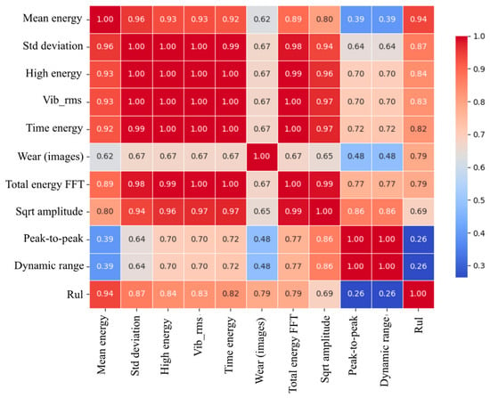
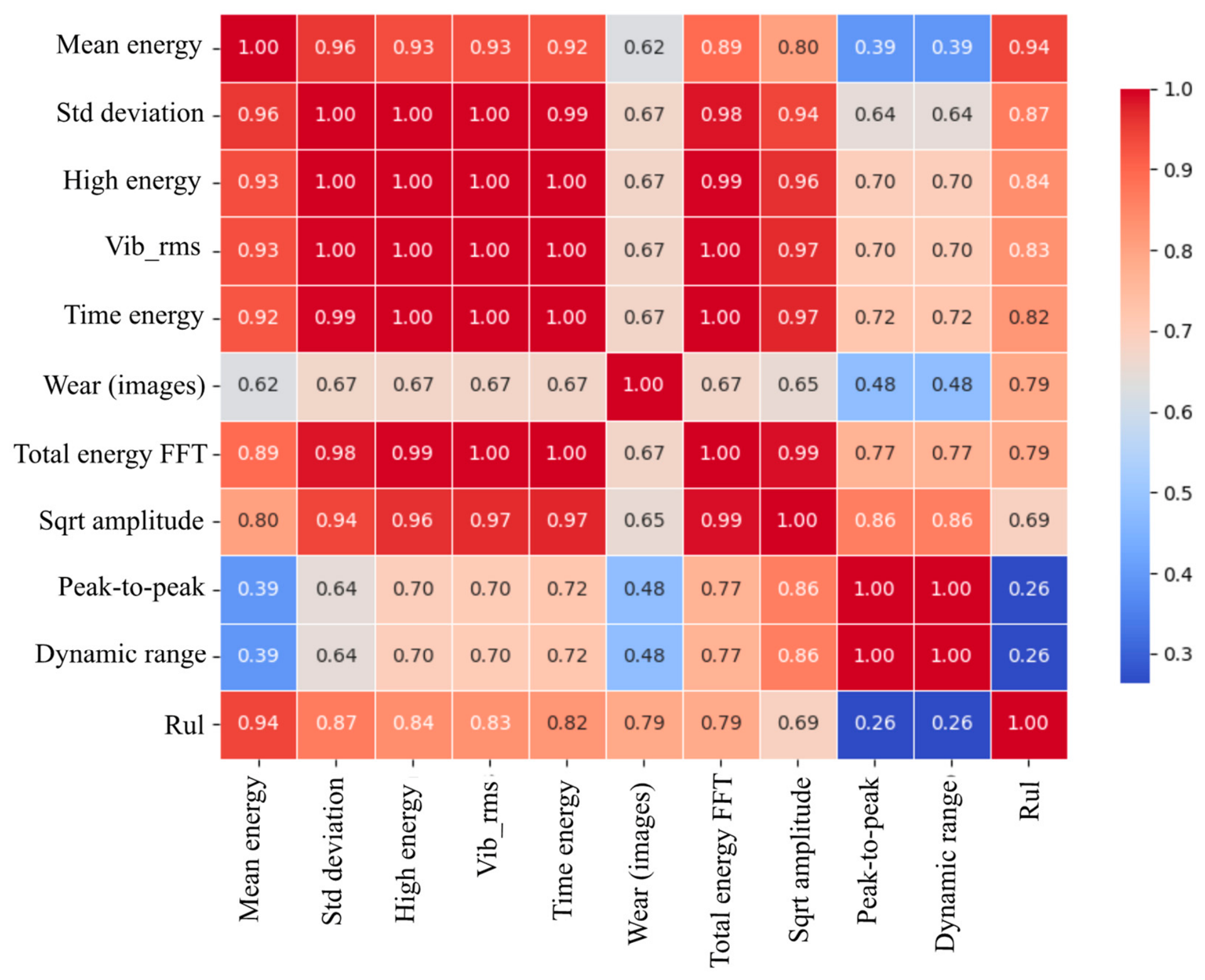
The correlation analysis between the main vibration characteristics and RUL revealed significant patterns that validate the experimental methodology. Figure 8 presents the correlation heatmap between all analyzed variables.
Figure 8.
Heat map of correlation between the main vibration characteristics (top 10) and RUL.
The mean vibration energy proved to be the most reliable macroscopic indicator of wear progression, with a global correlation coefficient of 94.0% with the RUL across the complete 2460-cycle dataset. The standard deviation showed a correlation of 87.0%, while the RMS value reached a correlation of 83.0%. These results indicate that the energetic characteristics of the vibration signal are highly sensitive to the cumulative evolution of surface damage. However, as analyzed in Section 4, this single scalar metric simultaneously encapsulates both wear-induced impacts and kinetic energy variations from the three tested operating speeds (0.75, 1.15, and 1.40 m/s), requiring multivariate spectral and visual features to decouple both effects during active operation.
Particularly relevant is the Pearson correlation coefficient of obtained between the optical surface damage ratio and the target operational countdown (RUL). While contact fatigue and microcrack propagation exhibit localized stochastic bursts, this high correlation demonstrates a strong, global tracking between optical surface degradation and accumulated running cycles, validating as an effective physical input descriptor to complement vibration telemetry within the multimodal regression network.
The correlation analysis also revealed a strong linear dependence among most vibration characteristics, with values exceeding 96.0%. This behavior indicates that the information in these variables is redundant, justifying the use of dimensionality reduction techniques such as PCA to improve computational efficiency without affecting estimate accuracy.
Conversely, amplitude characteristics such as peak-to-peak value and dynamic range showed a weak correlation with RUL (r = 0.26), suggesting they are unreliable indicators of wheel wear. These results reinforce the usefulness of the vibration energy components, which demonstrated greater sensitivity to the evolution of surface damage.
3.3. Results of the PCA+SVM Model
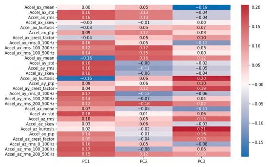
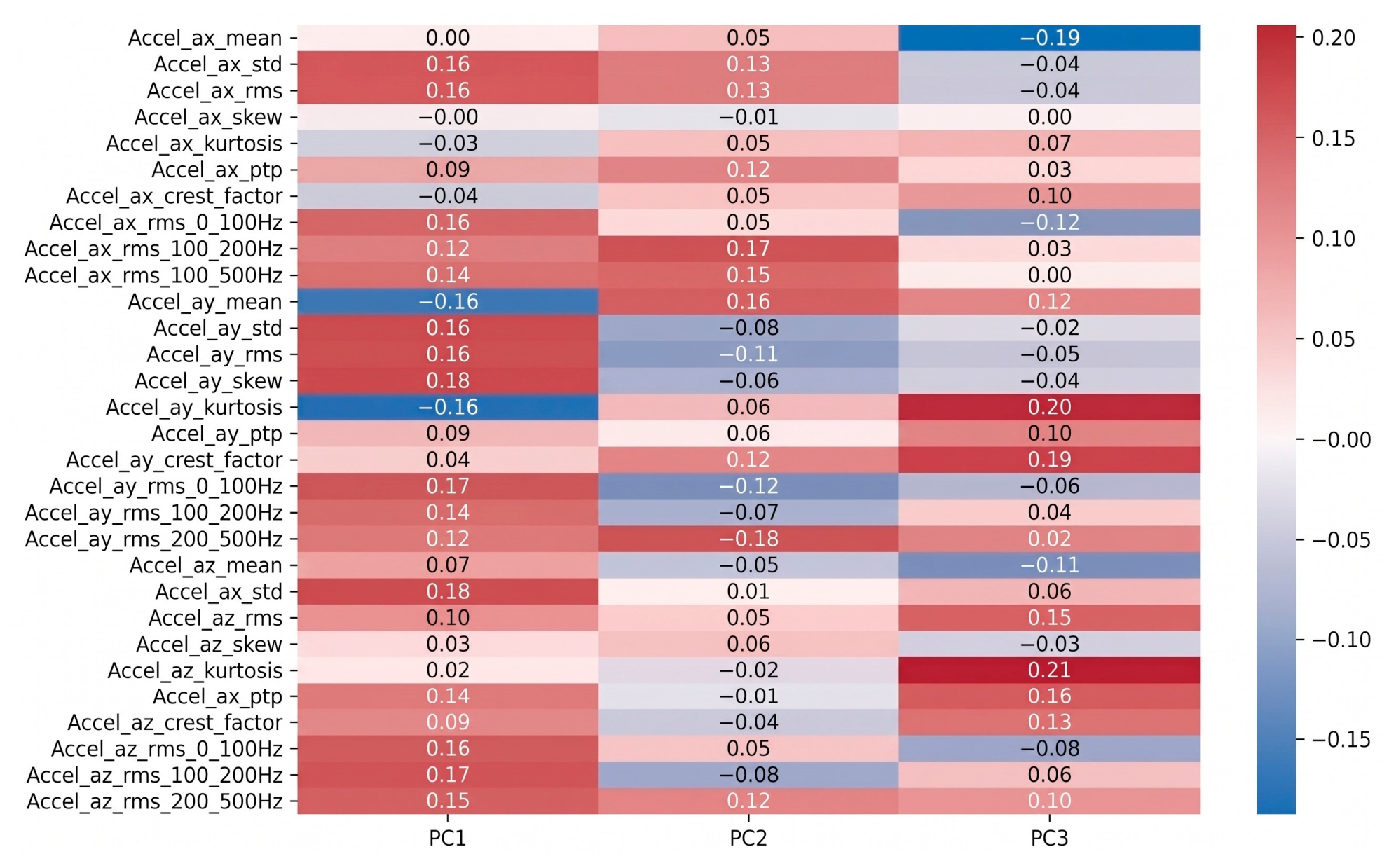
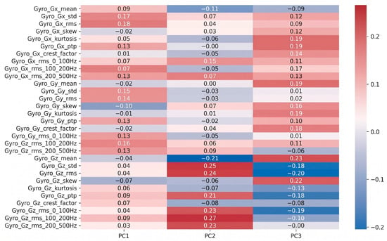
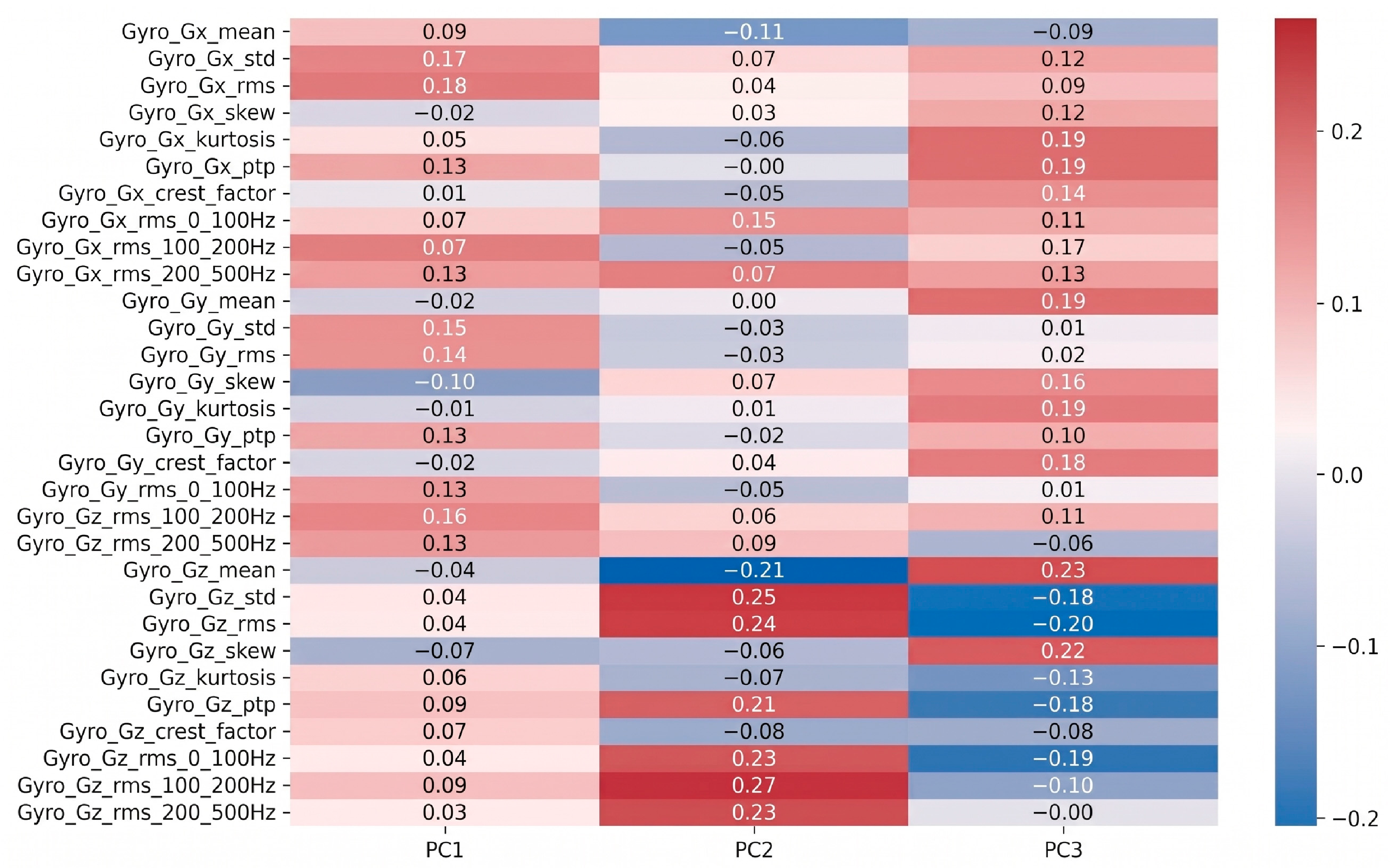
PCA extracted the most representative dynamic signatures of wear evolution, reducing the original vector of 60 time and frequency characteristics to a three-dimensional subspace. Figure 9 and Figure 10 display PCA factor loadings rather than correlation coefficients. The absolute magnitude indicates feature importance (magnitudes near zero denote negligible influence, while indicate dominant variables), with algebraic signs representing projection orientation along each principal component. Analysis of the loadings heat maps revealed key physical correlations between vehicle dynamics and surface damage, as illustrated in Figure 9 for acceleration signals and Figure 10 for rotational (gyroscope) signals:
Figure 9.
Heat map of PCA factor loadings for acceleration signals across the first three principal components (PC1–PC3). Magnitudes represent projection weights (relative contribution) of each feature; values near zero indicate negligible influence, while large absolute values designate dominant physical descriptors.
Figure 10.
Heat map of PCA factor loadings for rotational (gyroscope) signals across the first three principal components (PC1–PC3).
- The First Principal Component (PC1) is predominantly governed by the low-frequency band (0–100 Hz) of acceleration signals along with pitch and roll motions (Figure 9 and Figure 10). From a kinematic standpoint, given the wheel diameter ( mm) and the experimental speed range ( to m/s), the fundamental rotational frequency of the wheelsets () spans between 5.31 Hz and 9.90 Hz, with its primary harmonics () falling below 30 Hz. Furthermore, based on the secondary suspension stiffness ( N/mm) and the vehicle mass ( kg), the rigid-body bounce and pitch natural frequencies of the carbody lie within this sub-30 Hz regime. Consequently, PC1 physically captures the global rigid-body response of the suspension excited by the generalized increase in track-wheel surface roughness.
- The Second Principal Component (PC2) shows prominent factor loadings in the mid-frequency band (100–200 Hz), particularly for yaw angular velocity ( from the gyroscope Z-axis) (Figure 10). In railway dynamics, non-uniform annular wear alters the effective rolling radius difference between paired wheels, inducing lateral creepage fluctuations and periodic hunting oscillations. The 100–200 Hz band matches the structural yaw modes of the miniature bogie frame under wheelset slip guidance constraints, making PC2 an effective kinematic indicator of differential surface degradation.
- The Third Principal Component (PC3) exhibits dominant loadings in waveform impulsiveness metrics (namely kurtosis and crest factor in vertical and lateral accelerations) coupled with the high-frequency band (200–500 Hz) (Figure 9). Mechanically, as localized microcracks, pits, and spalling traverse the narrow Hertzian contact patch ( mm), they produce sharp impact shocks of sub-millisecond duration ( ms). In signal processing, repetitive mechanical shocks skew vibration distributions into heavy-tailed profiles, sharply increasing kurtosis above the Gaussian baseline (kurtosis 3) and exciting structural ringing up to the Nyquist limit (500 Hz at kHz). PC3 therefore isolates transient surface fatigue shocks from continuous background noise.
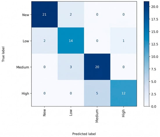
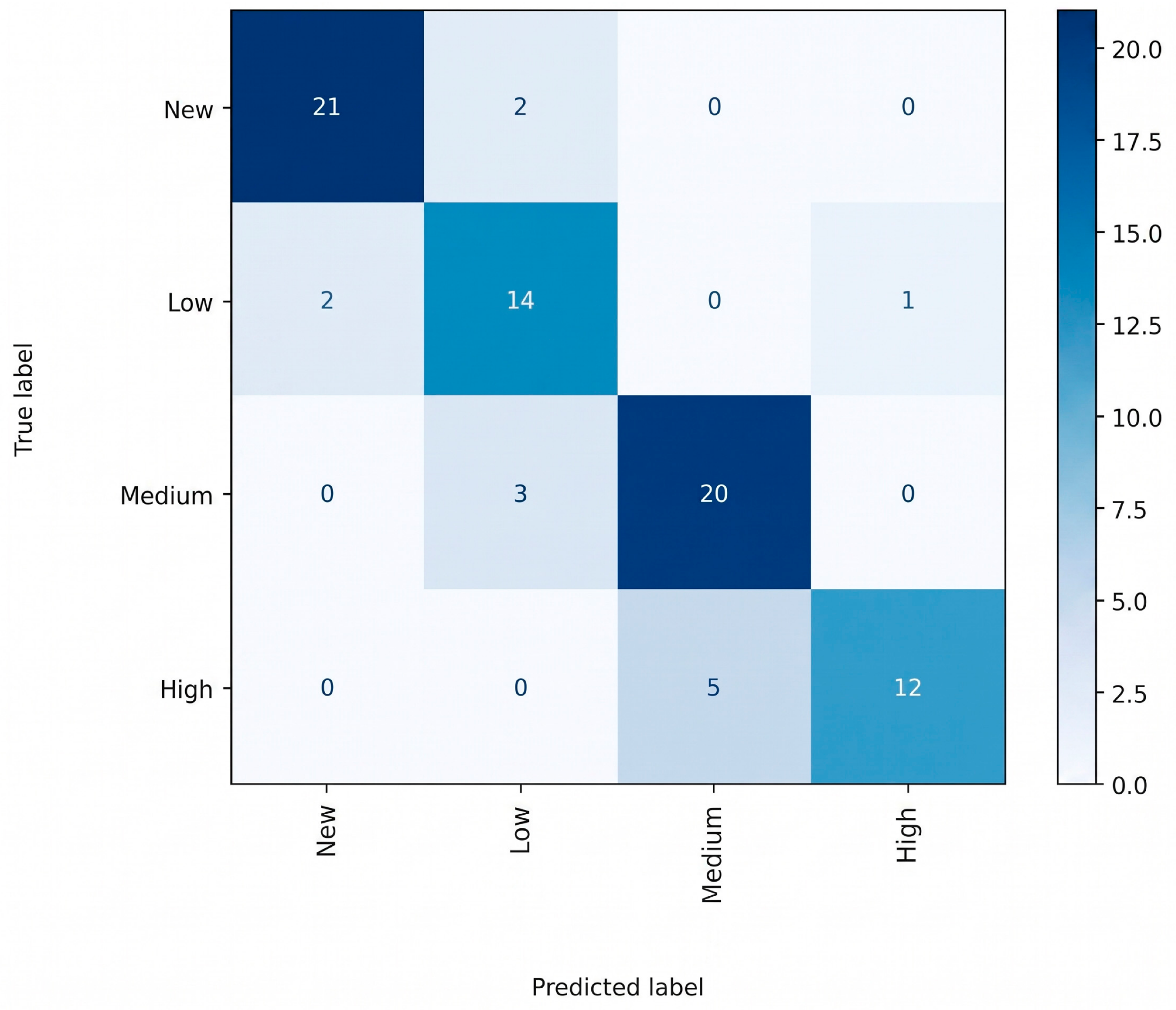
For diagnostic performance, the SVM classifier trained on projections onto these three principal components achieved an overall accuracy of 84% in categorizing the four operating states. As shown in the confusion matrix in Figure 11, the model effectively separates the new-wheel class, and misclassifications occurred almost exclusively between adjacent wear states (low and medium states). This behavior confirms that the model accurately captures the failure’s evolutionary trend. However, the 84% accuracy limit indicates that aggressively compressing the feature space (from 60 variables to only 3 dimensions) sacrifices fundamental degrees of freedom needed to mathematically resolve overlap in the more complex data.
Figure 11.
Confusion matrix of the SVM classifier trained with the first three principal components.
3.4. FCNN Model Results
To help prevent overfitting on the dataset of 240 images, data augmentation was applied to the vibration signals using time shifting (±5 samples) and Gaussian noise injection (SNR = 30 dB). This strategy expanded the training set to 1920-time windows, allowing the FCNN architecture to generalize adequately without compromising embedded computing capacity.
The FCNN implemented for continuous RUL regression performed exceptionally well. The multimodal input of 23 features (22 vibrations features + 1 wear feature per image) allowed the model to learn the nonlinear relationships between dynamic signals and wear progression.
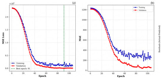
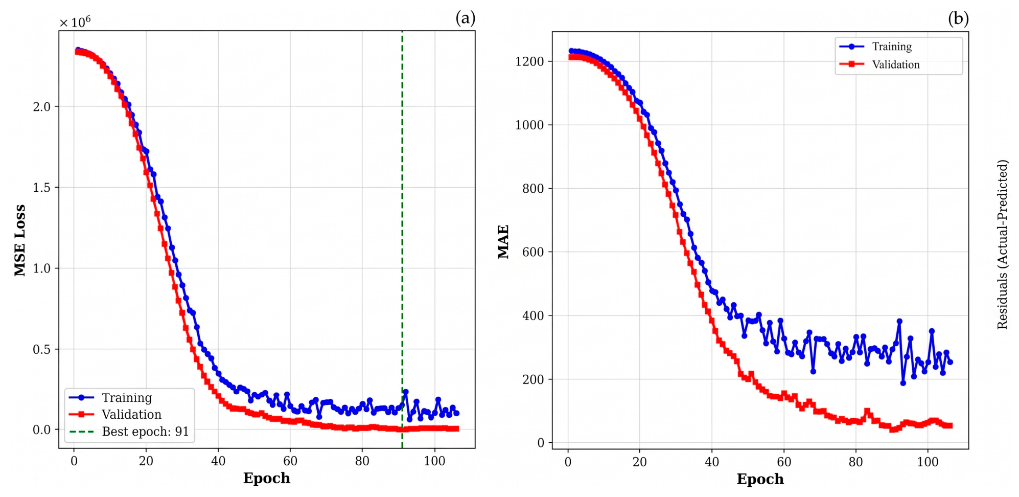
Figure 12a describes the evolution of the MSE loss function (as mathematically defined in Equation (6)) during training. Both training and validation losses decrease continuously until stabilizing around epoch 110, with no evidence of overfitting. The close relationship between the two curves confirms robust generalization to unseen data. While the training error initially decreases as computational effort (epochs) increases, the minimum achievable error is physically bounded by the intrinsic stochastic noise of the wear process. The Early Stopping mechanism ensures the model learns the underlying physics rather than overfitting to this noise.
Figure 12.
FCNN model behavior: (a) Evolution of the loss during training; (b) Mean absolute error per epoch.
To evaluate the model’s predictive performance on the unseen test set, the MAE was introduced and calculated as follows:
where is the actual remaining useful life, is the predicted remaining useful life, and represents the total number of samples evaluated in the independent test set ( 48). Applying this metric, the model achieved an MAE of 100 cycles in RUL estimation across the test set (Figure 12b). It is critical to emphasize that this MAE represents the average prediction error across all intermediate operational stages present in the test set (continuously predicting remaining cycles from 2460 down to 0) rather than a single prediction of the terminal threshold. The network acts as a continuous regressor, tracking the degradation trajectory throughout the entire lifespan.
Across the total operational lifespan of 2460 cycles (), this deviation corresponds to a Normalized Mean Absolute Error (NMAE) of 4.06%. The NMAE provides a relative percentage of the error normalized against the maximum defined life cycle, calculated as:
This relative error margin of approximately 4% indicates high prognostic precision for rolling contact fatigue applications.
It is worth noting the distinct operational domains of the two evaluated models: while the PCA+SVM pipeline operates as a discrete four-state classifier (achieving an 84% state classification accuracy), the FCNN model functions as a continuous prognostic regressor, estimating the remaining cycle count with an average uncertainty margin of only . Residual analysis showed a zero-mean random dispersion without systematic bias, confirming that the network generalized the multimodal feature space reliably without overfitting.
3.5. Comparative Analysis of Models
The results in Table 2 show a balance between both approaches. The PCA+SVM model offers an interpretable diagnosis and accurate classification of discrete wear states, enabling category-based maintenance decisions. In contrast, FCNN provides a more granular RUL estimate, enabling more precise and optimized maintenance scheduling.
Table 2.
Comparative summary of model performance.
PCA loading analysis identifies high-frequency energy and kurtosis as the physical precursors of fatigue wear. This physical interpretability is a key advantage of the PCA+SVM model, as it lets engineers understand which aspects of system dynamics indicate proximity to failure.
4. Discussion
The results obtained in this work show that the selection of an artificial intelligence strategy for predictive railway maintenance depends strictly on the operational objective of the application:
- a diagnosis based on discrete categorization
- a quantitative forecast of useful life.
These findings partially align with recent studies. For example, Iliopoulos and Sakellariou [38] estimated the RUL of railway wheels using onboard random vibrations, achieving errors of less than 5% under controlled conditions, but without merging visual information. Meanwhile, Mosleh et al. [11] used SVM with experimental wear data, achieving similar accuracies (%) in severity classification, but relied only on force signals and did not leverage multimodality. The main contribution of this work compared to these studies is incorporating visual wear quantification as ground truth and multimodal fusion, which enables cross-validation between physical domains (mechanical and optical).
Meanwhile, the FCNN has emerged as the superior approach for continuous RUL estimation. Although individual features such as mean vibration energy exhibit a strong global linear correlation with RUL () across the entire lifecycle, a simple univariate linear regression model () is insufficient for multi-speed operational environments. The underlying physical limitation is that, during operation, the total measured vibration energy is a composite signal governed simultaneously by the vehicle’s kinetic energy (operating speed, evaluated at m/s) and the tribological surface degradation, such that (). Because the explicit vehicle speed is not provided as an external input, a univariate regression model relying solely on a single scalar energy value cannot know what fraction of the measured energy stems from the kinetic speed regime and what fraction corresponds to actual surface wear. Consequently, a mildly worn wheel operating at high speed (1.40 m/s, high kinetic energy) can generate a total mean vibration energy level identical to that of a severely degraded wheel operating at low speed (0.75 m/s, low kinetic energy), causing a univariate model to erroneously interpret a routine speed increase as an immediate drop in RUL.
In contrast, the FCNN resolves this operational ambiguity without requiring a dedicated speed sensor by leveraging the full 23-feature multimodal input vector (comprising 12 time-domain metrics, 7 FFT spectral sub-bands from 0 to 500 Hz, spectral centroid, dominant harmonic peak, total FFT energy, and the optical worn area . Physically, kinetic speed changes and surface wear excite distinct regions of the frequency spectrum: variations in vehicle speed predominantly shift energy within the low-frequency rigid-body suspension bands (0–100 Hz), whereas progressive surface distress (pitting, microcracking, and spalling) generates transient contact shocks that selectively amplify high-frequency spectral energy (200–500 Hz) and waveform impulsiveness (kurtosis and crest factor), which are further corroborated by the visual metric . By simultaneously evaluating the distribution of energy across low and high frequency bands alongside , the FCNN implicitly accounts for the kinetic contribution and isolates the true wear-induced degradation. It maps these complex, nonlinear interactions with high accuracy (%), achieving stable convergence and a random distribution of residuals without systematic bias. This granular forecasting capability allows for more flexible intervention scheduling than traditional static threshold systems.
The relaxation of strict dynamic similarity introduces key physical implications when translating these laboratory findings to industrial railway operations. Operating without full Froude scaling () shifts rigid-body resonance frequencies (scaled theoretically by ) and alters dynamic contact amplification, meaning that raw vibration thresholds and spectral boundaries cannot be directly mapped to commercial revenue speeds. Furthermore, using AA7075-T6 aluminum instead of hardened railway steel intentionally accelerates contact fatigue mechanisms, meaning that the 2460 test cycles represent controlled laboratory degradation milestones rather than operational mileage.
Consequently, the core contribution of this work is methodological rather than empirical parameter calibration. While neural network weights require retraining for full-scale deployments, the fundamental monitoring framework remains directly transferable: the dual-tier architecture (edge-level PCA+SVM classification paired with cloud-level FCNN prognosis) and the physical feature hierarchy (where low frequencies capture generalized profile wear and high-frequency kurtosis flags localized contact fatigue). For commercial implementation, transfer learning and multi-body dynamic simulations can bridge the dynamic scale gap to recalibrate these models using on-track axlebox telemetry.
Regarding the transferability of the physical parameters for future research, the geometric parameters can be directly scaled to full-scale rolling stock using similarity laws (). However, scaling dynamic wear rates and RUL to industrial steel wheels requires addressing two scaling gaps: (i) stiffness and material wear resistance (AA7075-T6 vs. standard UIC steel grades like R260), and (ii) contact stress scaling. Future investigations will aim to calibrate transfer functions based on energy-dissipation scaling laws (e.g., or Archard index mappings), allowing dynamic thresholds identified in scaled experiments (such as high-frequency kurtosis emergence in PC3) to serve as normalized dimensionless health indicators for full-scale bogies.
5. Conclusions
This study demonstrated the feasibility of implementing two complementary artificial intelligence approaches for monitoring wear on railway wheels, using a 1:20 scale instrumented vehicle. On the one hand, the FCNN proved highly effective for continuous estimation of RUL, achieving high accuracy and generalizability by merging longitudinal vibration characteristics with surface wear quantified using machine vision. On the other hand, the hybrid PCA+SVM model validated its operational utility for diagnosing discrete failure states and, crucially, provided physical interpretability to the process. PCA identified high-frequency energy and waveform changes (kurtosis) as the most reliable dynamic precursors of wear severity.
The choice between these architectures will depend on the required maintenance strategy: FCNN is ideal for optimized and quantitative long-term planning, while PCA+SVM is suitable for diagnostics where auditing the physical origin of the failure is required. Although the controlled laboratory environment was fundamental for establishing an accurate correlation between vibration and physical degradation, future work should focus on transferring this methodology to full-scale railway environments. This will involve recalibrating the models to account for the stochastic noise of commercial tracks, environmental variations, and the mechanical properties of industrial steel, thus consolidating a comprehensive predictive maintenance system.
From an operational perspective, the results suggest that a hybrid system could be implemented in two layers: an edge layer (PCA+SVM, 84% accuracy) for early alerts of state change, and a cloud layer (FCNN, ) for strategic maintenance planning, potentially reducing inspection costs by at least 30% compared to traditional visual methods.
Author Contributions
T.E.S.V., J.E.L.R. and G.M.S.F. conceived and designed the experiment; T.E.S.V. performed the analysis, interpreted the data, and wrote the original draft; G.H.-H. developed the instrumentation and the scaled railway vehicle for data acquisition; J.E.B.-S. reviewed the methodology and contributed to the statistical design; F.V.-M. and J.C.J.-C. supervised the research, revised the manuscript, and gave final approval for submission. All authors have read and agreed to the published version of the manuscript.
Funding
This research was funded by SECIHTI, grant number CF-2023-I-204, and Postdoctoral stays in Mexico 2022 (3), 2023 (1) and 2025 (1).
Data Availability Statement
The original contributions presented in the study are included on the Kaggle page (https://www.kaggle.com/railwayuaq, accessed on 30 October 2026); further inquiries can be directed to the corresponding author.
Acknowledgments
The authors would like to thank SECIHTI for supporting this work.
Conflicts of Interest
The authors declare no conflicts of interest.
Abbreviations
The following abbreviations are used in this manuscript:
| ANOVA | Analysis of Variance |
| CF | Crest Factor |
| CNNs | Convolutional Neural Networks |
| FCNN | Fully Connected Neural Network |
| FFT | Fast Fourier Transform |
| IMU | Inertial Measurement Unit |
| MAE | Mean Absolute Error |
| MLP-RF | Multilayer Perceptron + Random Forest |
| MSE | Mean Squared Error |
| NMAE | Normalized Mean Absolute Error |
| PCA | Principal Component Analysis |
| RBF | Radial Basis Function |
| RMS | Root Mean Square |
| ROI | Region of Interest |
| RUL | Remaining Useful Life |
| SNR | Signal-to-Noise Ratio |
| SVM | Support Vector Machines |
| UIC | International Union of Railways |
References
- Aboul-Atta, T.A.; Elmaraghy, S.B.E. Factors affecting performance improvement of the metro system in cities. J. Eng. Appl. Sci. 2022, 69, 27. [Google Scholar] [CrossRef] [Scilit]
- Zhu, Y.; Wang, T.; Shen, R.; Xie, J.; Yang, J.; Zhang, G.; Tian, H.; Liang, X. Development and engineering application of integrated safety monitoring systems for China’s high-speed trains. Transp. Saf. Environ. 2024, 6, tdad017. [Google Scholar] [CrossRef] [Scilit]
- Gobierno de México. Plan Nacional Ferroviario: Proyectos Estratégicos 2024–2030; Presidencia de la República: Ciudad de México, México, 2024. Available online: https://www.gob.mx/cms/uploads/attachment/file/1021187/09_PS_SICT_2025-2030.pdf (accessed on 15 March 2026).
- International Union of Railways (UIC). UIC Safety Report 2025: Significant Accidents 2024; UIC: Paris, France, 2025; Available online: https://uic.org/safety (accessed on 15 March 2026).
- Cruz, A.L. Van Más de 7 Mil Siniestros en Trenes en Cinco Años. EL UNIVERSAL, Ciudad de México, 3 January 2026; Available online: https://www.eluniversal.com.mx/nacion/van-mas-de-7-mil-siniestros-en-trenes-en-cinco-anos/ (accessed on 15 March 2026).
- Carabaña, C. Viaje a la Tragedia del Tren Interoceánico. EL PAÍS, Madrid, 27 January 2026. Available online: https://elpais.com/mexico/2026-01-28/viaje-a-la-tragedia-del-tren-interoceano.html (accessed on 15 March 2026).
- Kumar, A.; Harsha, S.P. A systematic literature review of defect detection in railways using machine vision-based inspection methods. Int. J. Transp. Sci. Technol. 2024, 18, 207–226. [Google Scholar] [CrossRef] [Scilit]
- Li, P.; Wang, L.; Lan, C.; Sun, X.; He, Z.; Liu, Z. Mapping Rail-Joint Straightness to Passenger Ride Comfort via Field Measurement and Multibody Dynamic Modelling. Vehicles 2025, 7, 148. [Google Scholar] [CrossRef] [Scilit]
- Zhao, C.; Fan, Z.; Li, P. Research on the Dynamic Response Characteristics of a Railway Vehicle Under Curved Braking Conditions. Vehicles 2025, 7, 18. [Google Scholar] [CrossRef] [Scilit]
- Lei, Y.; Li, N.; Gontarz, S.; Lin, J.; Radkowski, S.; Dybala, J. Machinery health prognostics: A systematic review from data acquisition to RUL prediction. Mech. Syst. Signal Process. 2018, 104, 799–834. [Google Scholar] [CrossRef] [Scilit]
- Mosleh, A.; Meixedo, A.; Ribeiro, D.; Montenegro, P.; Calçada, R. Machine learning approach for wheel flat detection of railway train wheels. Transp. Res. Procedia 2023, 72, 4199–4206. [Google Scholar] [CrossRef] [Scilit]
- Jardine, A.K.S.; Lin, D.; Banjevic, D. A review on machinery diagnostics and prognostics implementing condition-based maintenance. Mech. Syst. Signal Process. 2006, 20, 1483–1510. [Google Scholar] [CrossRef] [Scilit]
- Wang, X.; Li, K.; Chehri, A. Multi-sensor fusion technology for 3D object detection in autonomous driving: A review. IEEE Trans. Intell. Transp. Syst. 2023, 25, 1148–1165. [Google Scholar] [CrossRef] [Scilit]
- Shaikh, K.; Hussain, I.; Chowdhry, B.S. Wheel defect detection using a hybrid deep learning approach. Sensors 2023, 23, 6248. [Google Scholar] [CrossRef] [Scilit] [PubMed]
- Wan, T.H.; Tsang, C.W.; Hui, K.; Chung, E. Anomaly detection of train wheels utilizing short-time Fourier transform and unsupervised learning algorithms. Eng. Appl. Artif. Intell. 2023, 122, 106037. [Google Scholar] [CrossRef] [Scilit]
- García-Troya, M.; Sánchez-Lozano, M.; Abellán-López, D. Development and Verification of a FEM Model of Wheel–Rail Contact, Suitable for Large Parametric Analysis of Independent Guided Wheels. Vehicles 2025, 7, 104. [Google Scholar] [CrossRef] [Scilit]
- Chung, K.-J.; Lin, C.-W. Condition monitoring for fault diagnosis of railway wheels using recurrence plots and convolutional neural networks (RP-CNN) models. Meas. Control 2024, 57, 330–338. [Google Scholar] [CrossRef] [Scilit]
- Winarno, A.; Sandhy, R.I.D.; Nazmi, N.; Priatomo, H.R.; Suwastono, A.; Charisma, G.E.; Bahiuddin, I. Roles of Vibration-Based Machine Learning Algorithms in Railway Vehicle Monitoring for Track Condition Assessment: A Review. J. Vib. Eng. Technol. 2025, 13, 242. [Google Scholar] [CrossRef] [Scilit]
- Zhao, R.; Yan, R.; Chen, Z.; Mao, K.; Wang, P.; Gao, R.X. Deep learning and its applications to machine health monitoring: A survey. Mech. Syst. Signal Process. 2019, 115, 213–237. [Google Scholar] [CrossRef] [Scilit]
- Gómez, M.J.; Castejón, C.; Corral, E.; García-Prada, J. Railway Axle Condition Monitoring Technique Based on Wavelet Packet Transform Features and Support Vector Machines. Sensors 2020, 20, 3575. [Google Scholar] [CrossRef] [Scilit] [PubMed]
- Deng, L.-F.; Zhang, A.; Zhao, R. Intelligent identification of incipient rolling bearing faults based on VMD and PCA-SVM. Adv. Mech. Eng. 2022, 14, 168781402110729. [Google Scholar] [CrossRef] [Scilit]
- Pryma, J.; Knap, P.; Lalik, K. Deployment-Aware Comparison of Classical Machine Learning and 1D CNN for Bearing Fault Diagnosis on Embedded Hardware. In 2026 27th International Carpathian Control Conference (ICCC); IEEE: Washington, DC, USA, 2026; pp. 384–389. [Google Scholar]
- Pule, M.; Matsebe, O.; Samikannu, R. Application of PCA and SVM in Fault Detection and Diagnosis of Bearings with Varying Speed. Math. Probl. Eng. 2022, 2022, 5266054. [Google Scholar] [CrossRef] [Scilit]
- Song, X.; Zhang, Q.; Sun, R.; Tian, R.; Sun, J.; Li, C.-X.; Cui, Y.-X. A Hybrid Deep Learning Prediction Method of Remaining Useful Life for Rolling Bearings Using Multiscale Stacking Deep Residual Shrinkage Network. Int. J. Intell. Syst. 2023, 2023, 6665534. [Google Scholar] [CrossRef] [Scilit]
- Shang, J.; Xu, D.; Qiu, H.; Gao, L.; Jiang, C.; Yi, P. A novel data augmentation framework for remaining useful life estimation with dense convolutional regression network. J. Manuf. Syst. 2024, 74, 30–40. [Google Scholar] [CrossRef] [Scilit]
- Archard, J.F. Contact and Rubbing of Flat Surfaces. J. Appl. Phys. 1953, 24, 981–988. [Google Scholar] [CrossRef] [Scilit]
- Wang, L.-L.; Wu, M.-H. Research on bearing fault diagnosis based on machine learning and SHAP interpretability analysis. Sci. Rep. 2025, 15, 41242. [Google Scholar] [CrossRef] [Scilit] [PubMed]
- Bodini, I.; Petrogalli, C.; Faccoli, M.; Mazzù, A. Vision-based damage analysis in shoe-braking tests on railway wheel steels. Wear 2022, 506–507, 204514. [Google Scholar] [CrossRef] [Scilit]
- Chang, H.; Borghesani, P.; Smith, W.A.; Peng, Z. Application of surface replication combined with image analysis to investigate wear evolution on gear teeth—A case study. Wear 2019, 430–431, 355–368. [Google Scholar] [CrossRef] [Scilit]
- Schlagenhauf, T.; Scheurenbrand, T.; Hofmann, D.; Krasnikow, O. Analysis of the visually detectable wear progress on ball screws. CIRP J. Manuf. Sci. Technol. 2022, 39, 321–332. [Google Scholar] [CrossRef] [Scilit]
- Shashikala, T.; Sunitha, S.; Basavarajappa, S. Quantification of Worn Surface using Digital Image Processing. Tribol. Int. 2022, 176, 107864. [Google Scholar] [CrossRef] [Scilit]
- Kamratowski, M.; Janßen, C.; Davidovic, M.; Bergs, T. Quantification of wear on gear cutting tools using computer vision methods. Forsch. Ingenieurwes. 2025, 89, 12. [Google Scholar] [CrossRef] [Scilit]
- Johnson, K.L. Contact Mechanics; Cambridge University Press: Cambridge, UK, 1985. [Google Scholar] [CrossRef] [Scilit]
- Goodfellow, I.; Bengio, Y.; Courville, A. Deep Learning; Chapter 6: Deep Feedforward Networks; MIT Press: Cambridge, MA, USA, 2016. [Google Scholar]
- Iwana, B.K.; Uchida, S. An Empirical Survey of Data Augmentation for Time Series Classification with Neural Networks. PLoS ONE 2021, 16, e0254841. [Google Scholar] [CrossRef] [Scilit] [PubMed]
- Abdi, H.; Williams, L.J. Principal Component Analysis. Wiley Interdiscip. Rev. Comput. Stat. 2010, 2, 433–459. [Google Scholar] [CrossRef] [Scilit]
- Cristianini, N.; Shawe-Taylor, J. An Introduction to Support Vector Machines and Other Kernel-Based Learning Methods; Cambridge University Press: Cambridge, UK, 2000. [Google Scholar] [CrossRef] [Scilit]
- Iliopoulos, I.A.; Sakellariou, J.S. Remaining Useful Life Estimation of Hollow Worn Railway Vehicle Wheels via On-Board Random Vibration-Based Wheel Tread Depth Estimation. Sensors 2024, 24, 375. [Google Scholar] [CrossRef] [Scilit] [PubMed]

Disclaimer/Publisher’s Note: The statements, opinions and data contained in all publications are solely those of the individual author(s) and contributor(s) and not of MDPI and/or the editor(s). MDPI and/or the editor(s) disclaim responsibility for any injury to people or property resulting from any ideas, methods, instructions or products referred to in the content. |
© 2026 by the authors. Licensee MDPI, Basel, Switzerland. This article is an open access article distributed under the terms and conditions of the Creative Commons Attribution (CC BY) license.