


Abstract
This paper presents the design, implementation, and Sim-to-Real evaluation of a Nonlinear Model Predictive Control (NMPC) strategy for autonomous urban shuttles and last-mile transport, focusing on bridging the reality gap. A decoupled NMPC architecture was developed for a by-wire Toyota Prius, explicitly compensating for a measured 100 ms steering actuator delay. The system was first evaluated in the CARLA simulation environment and subsequently deployed on the physical vehicle under matching operational conditions. Real-world trials confirmed consistent transfer of the core control logic, evidenced by a high correlation in steering commands (). However, a systematic Cross-Track Error (CTE) offset (averaging ) was observed. An in-depth gap diagnosis suggests that this tracking discrepancy was primarily driven by real-world yaw angle sensor bias and variability rather than fundamental flaws in the NMPC algorithm itself. Building on this diagnosis, controller refinements—including the use of a path-derived yaw input and an alternative formulation providing integral action—were designed and evaluated within the simulation environment (with physical deployment remaining as future work). In CARLA, these refinements significantly improved tracking accuracy, reducing mean absolute CTE from to . Finally, a systematic parameter sensitivity analysis in CARLA provides practical tuning guidelines. Overall, the study highlights how high-fidelity simulation can support controller development and diagnostic root cause isolation, while emphasizing the critical interplay between control design, state estimation fidelity, and hardware characteristics in Sim-to-Real deployment.
1. Introduction
Autonomous vehicle controllers must ensure accurate trajectory tracking while accounting for model mismatch, sensor noise, and actuator delays. Nonlinear Model Predictive Control (NMPC) has emerged as an interesting framework to handle these complexities by incorporating multi-variable constraints and explicit future behavior prediction [1]. While high-fidelity simulators offer safe environments for development, the Sim-to-Real gap—arising from unmodeled dynamics and sensor imperfections—remains a persistent challenge that degrades real-world performance if left unaddressed. Bridging this gap requires not only robust controller design, but also systematic methods to quantify and diagnose the sources of mismatch.
This paper addresses these challenges through the design and Sim-to-Real gap evaluation of a latency-aware NMPC architecture for a by-wire autonomous research vehicle. The system explicitly compensates for a measured 100 ms steering delay and was tested both in simulation and on the physical vehicle under matching conditions at speeds (4 m/s and 5 m/s) representative of autonomous shuttles and last-mile transport vehicles—a speed regime similarly adopted in recent real-world Sim-to-Real control studies [2]. The Sim-to-Real gap is quantitatively measured through a systematic comparison. Unlike End-to-End (E2E) deep learning approaches—which operate as uninterpretable “black boxes” where perception, planning, and control failures cannot be easily disentangled [3]—a modular paradigm is adopted in this work. By keeping state estimation, reference processing, and NMPC optimization explicitly separated, this modular setup provides the transparency needed to quantitatively isolate hardware anomalies from control logic flaws.
By utilizing a kinematic model where tire slip is negligible, this study finds that observed discrepancies in Cross-Track Error (CTE) primarily originate from yaw angle sensor bias rather than from the control algorithm itself. This diagnostic approach helps isolate hardware-level issues from control logic, providing a testbed for evaluating control strategies and diagnostic procedures within the target operational domain, under the tested low-speed closed-circuit conditions.
This study is guided by four primary research questions: (RQ1) What is the Sim-to-Real gap between a Latency-Aware NMPC deployed in a state-of-the-art simulator for autonomous driving research (CARLA) and a physical vehicle?; (RQ2) What is the primary source of the Cross-Track Error discrepancy observed when transferring a Latency-Aware NMPC controller from high-fidelity simulation to a physical vehicle?; (RQ3) Can targeted controller refinements, informed by this diagnosis, measurably mitigate the identified sensor-induced tracking errors?; and (RQ4) How do key NMPC tuning parameters affect the trade-off between tracking accuracy and control smoothness under the tested operating conditions? Rather than proposing a new theoretical NMPC formulation, the novelty of this work lies in the systematic, empirically grounded diagnostic workflow used to answer these questions and in the transparent quantification of how the resulting refinements address the diagnosed root cause (further discussed in Section 2).
In summary, the main contributions of this work are as follows:
- Design, implementation and real-world deployment of a decoupled latency-aware NMPC architecture for lateral and longitudinal control that explicitly compensates for a measured 100 ms steering actuator delay using state augmentation.
- An empirical diagnostic workflow utilizing the CARLA simulator as a tool to trace the primary sources of the Sim-to-Real gap, identifying yaw angle measurement offset as a leading contributor to systematic CTE discrepancies.
- The design and simulation-based evaluation, at a target velocity of 4 m/s, of two key controller refinements aimed at mitigating the diagnosed hardware-induced errors: (a) a path-derived yaw input to mitigate the impact of sensor bias, and (b) a formulation to introduce integral action and improve steady-state error rejection and control smoothness.
- A systematic parameter sensitivity analysis (benchmarking) of the best-performing NMPC configuration among tested settings, providing practical tuning guidelines and generalizable insights regarding the trade-offs between tracking accuracy and control smoothness for key parameters such as the prediction horizon and cost function weights under the tested low-speed (4–5 m/s) closed-circuit conditions.
- A discussion contextualizing the Sim-to-Real findings and tuning results, offering recommendations for the development and deployment of NMPC in real-world autonomous vehicles facing similar hardware and latency limitations.
The remainder of this paper is organized as follows. Section 2 reviews related work. Section 3 details the complete controller design, including the alternative formulations, and the experimental setup. Section 4 presents the results, beginning with the baseline Sim-to-Real comparison, followed by the evaluation of controller refinements, and the parameter sensitivity analysis. Section 5 discusses the implications of these findings. Finally, Section 6 draws conclusions from the entire investigation and outlines directions for future work.
2. Related Work
2.1. Evolution of Vehicle Control Strategies
Control system design for autonomous vehicles has been extensively explored, with techniques ranging from classical methods to advanced optimization-based and learning-based strategies. Recent literature reviews [4,5] provide overviews of this evolution, detailing the trade-offs of classical control techniques, such as Proportional-Integral-Derivative (PID) controllers, which are widely adopted due to their simplicity and ease of implementation [6]. Similarly, geometric path tracking controllers like Pure Pursuit and Stanley have demonstrated reliable performance at low to moderate speeds [7]. However, these reactive methods often exhibit limitations in systematically handling dynamic constraints, optimizing performance over a predictive horizon, or managing the coupled, nonlinear behavior of vehicles in highly dynamic environments.
To overcome these limitations, a range of advanced strategies has been developed, primarily centered around optimal and robust control. While robust techniques (e.g., Sliding Mode Control [8,9]) and Lyapunov-based methods [10] focus on providing resilience against uncertainties and formal stability guarantees, a clear progression towards higher performance can be seen in optimization-based methods.
Strategies such as Linear Quadratic Regulators (LQR) compute a mathematically optimal state-feedback gain for a linear system, enhancing stability but offering no native mechanism for handling operational constraints. A direct evolution is Linear Model Predictive Control (LMPC), which introduces a predictive horizon and the crucial ability to handle constraints, making it highly effective for systems that can be accurately linearized [11,12,13,14]. However, the fundamental reliance of both LQR and LMPC on linearized models ultimately restricts their effectiveness in complex, highly nonlinear driving scenarios.
Nonlinear Model Predictive Control (NMPC), by contrast, directly addresses this limitation by explicitly accounting for nonlinear vehicle dynamics and operational constraints within its predictive model. This has led to its demonstrated superior performance in a wide range of applications, from highway trajectory planning [15] to complex obstacle avoidance maneuvers [16,17,18], dynamic urban driving [19,20,21], and high-fidelity multi-DOF trajectory tracking [22]. Although real-time execution has historically posed a significant challenge for NMPC, recent advances in embedded optimization techniques and efficient symbolic frameworks like CasADi [23], often paired with NLP solvers such as IPOPT [24], have effectively bridged this gap for real-world deployment.
Recently, data-driven approaches such as Deep Reinforcement Learning (DRL) and Imitation Learning (IL) have also gained traction for end-to-end or high-level vehicle control [3]. However, unless combined with additional constraint-handling or safety-verification layers, these learning-based techniques can pose challenges for formal constraint satisfaction, real-time safety guarantees, and interpretability compared to model-based predictive strategies like NMPC.
A comparative overview of these prevalent control strategies is presented in Table 1, highlighting the trade-offs that justify the selection of NMPC for this work.
Table 1.
Comparative Overview of Common Vehicle Control Strategies.
2.2. Bridging the Sim-to-Real Gap
High-fidelity simulation is essential for developing autonomous vehicles, serving as a scalable, repeatable, and cost-effective alternative to physical testing. Open-source platforms such as CARLA (Car Learning to Act) [25] have become foundational in academic and industrial research owing to their realistic physics engines, modular sensor suites, and flexible Python APIs [26]. Consequently, CARLA has been widely adopted for validating advanced control strategies, including Nonlinear Model Predictive Control (NMPC) [27,28,29].
Despite recent advances in virtual environments [30], a fundamental challenge persists: the discrepancy between simulated performance and real-world behavior, commonly referred to as the Sim-to-Real gap [31]. A digital twin, continuously updated with real-world data, is one prominent approach in the literature aimed at minimizing this gap [32]. This gap manifests across various stages of the autonomous driving pipeline, including perception [33], motion planning [34], control, and full-stack integration. For instance, a comprehensive full-stack framework (MCRPG) was proposed in [35] to evaluate and iteratively tune an entire Autonomous Driving Stack (ADS) encompassing perception, decision-making, planning, and control. Similarly, a full-stack platform methodology is presented in [36], specifically tailored to autonomous racing. In contrast to these multi-layer approaches, the present paper focuses on a targeted, algorithmic control-level study that diagnoses sensor-level root causes of reality gaps within a latency-aware NMPC system.
To quantify the Sim-to-Real gap in control models, existing literature predominantly relies on standard metrics such as Mean Absolute Error (MAE), Pearson Correlation Coefficient (PCC), and Cosine Similarity [37,38,39]. More recently, the -gap metric was proposed in [40]; however, its applicability is restricted to non-holonomic skid-steer differential drive robots.
As summarized in Table 2, existing Sim-to-Real control frameworks lack systematic diagnostic procedures to distinguish algorithmic model mismatches from physical hardware faults. As emphasized in [41], achieving a deeper understanding of the reality gap’s root causes is essential for effective mitigation. This work fills this gap by introducing a quantitative Cross-Track Error (CTE) diagnostic paradigm within the Sim-to-Real evaluation loop, providing actionable recommendations for seamless Sim-to-Real transfer of NMPC control in autonomous vehicles.
It is important to emphasize that individual NMPC components and delay compensation techniques are well-established in control literature. The value of this study lies not in introducing a novel theoretical NMPC formulation, but in demonstrating an empirical diagnostic workflow that leverages simulation to isolate and trace state-estimation imperfections (such as yaw sensor bias) from control logic errors in latency-compensated real-world deployments.
2.3. The Role of Actuator Latency
A particularly critical and tangible contributor to the Sim-to-Real gap is actuator latency, which can severely degrade controller performance and lead to instability if unmodeled. While this issue has been examined in various control contexts [42,43,44,45], its specific impact on the Sim-to-Real transfer of NMPC for full-scale passenger vehicles remains a key area of investigation. Recent works, such as the delay-aware robust control framework proposed by Kalaria et al. [46], have highlighted the complexity that latency introduces and the need for explicit compensation.
Overall, while the literature addresses NMPC, Sim-to-Real evaluation, and latency compensation individually, there is a notable absence of studies that integrate these elements into a unified diagnostic pipeline. Most existing works focus on error quantification or specific algorithm performance, often overlooking the systematic identification of hardware-level causes for the reality gap on full-scale by-wire vehicles. Table 2 provides a comparative overview of how this work fills these gaps relative to current state-of-the-art studies. By combining latency-aware design, rigorous performance comparison, and a quantitative diagnosis of hardware discrepancies, this investigation offers an end-to-end methodology for bridging the Sim-to-Real gap. The comparison works shown in Table 2 were selected as representative recent MPC/NMPC vehicle-control studies, already discussed above in Section 2, that report at least one of the three compared properties. Each property is defined explicitly for this comparison: a work is marked Latency-aware if it explicitly models or compensates for actuator or sensing delay within the controller design; Real-World Deployment if the proposed controller was tested on a physical, full-scale vehicle rather than only in simulation; and Root Cause Diagnosis if the study attributes an observed Sim-to-Real performance gap to a specific, isolated physical or sensing cause, rather than reporting an aggregate discrepancy metric alone.
Table 2.
Comparative Analysis of Related Literature in Autonomous Vehicle Control and Sim-to-Real Gap Diagnosis. ✓ indicates that the property is present for that work; ✗ indicates that it is not.
3. Methodology
This section details the design of the NMPC architecture depicted in Figure 1. It covers the formulation of the decoupled controllers, the mathematical models for vehicle dynamics including latency compensation, the definition of alternative controller formulations for performance analysis, and the configuration of both the simulated and real platforms.
Figure 1.
Sim-to-Real control architecture. The core NMPC algorithm (purple box) is deployed in two mutually exclusive execution environments: the physical vehicle platform (green box) and the high-fidelity simulation platform (cyan box).
3.1. NMPC Controller Design
The proposed control architecture consists of two decoupled NMPCs: one for lateral path tracking and one for longitudinal velocity regulation. This decoupled approach is adopted to prioritize the isolation and analysis of lateral Sim-to-Real discrepancies while ensuring real-time computational feasibility.
3.1.1. Lateral NMPC
The lateral controller is based on a discrete-time kinematic bicycle model. This approach is selected to align with the operating profiles of autonomous shuttles and last-mile transport vehicles. Given the low target operating speeds evaluated in this study (4–5 m/s) and the moderate curvature of the closed-circuit test track, lateral accelerations and the corresponding tire slip angles are expected to remain small, within the regime in which dynamic side-slip forces are commonly considered negligible relative to the vehicle’s kinematic motion. Consequently, the kinematic model captures the essential vehicle dynamics with fidelity while minimizing the computational complexity required for real-time optimization. As further shown in Section 4.2, the lateral deviations observed during real-world trials are traced to yaw angle estimation bias rather than to unmodeled tire dynamics or kinematic model mismatch, corroborating this modeling choice.
The controller operates with a sampling time of ms. This value is consistent with established architectural standards for high-level control in autonomous driving, which often balance sensor update rates and processing latency [46]. The physical steering actuator delay ( ms) was determined experimentally through step-response characterization tests on the vehicle, measuring the elapsed time between sending a CAN command from RTMaps and logging the initial wheel response via the TNO MOVE interface encoders. Since this delay equals one control time step, the actuator is modeled as a one-step delay, as experimental trials showed that state augmentation is necessary when . To capture this effect, the state vector is augmented with the current applied steering angle (), which lags the commanded angle () by one step, i.e.,
where is the vehicle position, the yaw angle, the linear velocity, and represents the steering angle physically applied to the wheels at step k, with being the discrete-time variable. The practical validity of this augmented delay representation is directly confirmed by the near-perfect command correlation () observed between simulation predictions and physical vehicle executions under matched conditions. The controller optimizes for the steering command , with dynamics given by
where L is the vehicle wheelbase, is the steering ratio (14.6 for the Toyota Prius) and is the longitudinal acceleration input provided by the longitudinal NMPC.
The cost function penalizes path-tracking error, yaw angle error, steering effort, steering rate and the state error in the terminal state as follows:
where is the prediction horizon, and are the cross-track and yaw angle errors, is the steering rate, and , , R, and S are weighting terms. The vector denotes terminal state errors. To promote closed-loop stability and state convergence, a terminal cost is applied, with as the stage-state weighting matrix.
A baseline set of weighting matrices was determined through initial empirical tuning in simulation to establish a conservative and safe starting point for the primary Sim-to-Real evaluation. Because real-world deployments involve unmodeled sensor noise and structural vibrations, these baseline values were intentionally selected to prioritize control smoothness and vehicle stability over aggressive tracking performance, yielding: , , and . This configuration assigns a significant penalty to the steering rate (S), damping potential high-frequency oscillations to ensure physical hardware safety during the initial trials. The terminal cost was set to to promote closed-loop stability.
3.1.2. Alternative Lateral Formulation: Implicit Integral Action via
To investigate performance improvements, particularly in steady-state error rejection under persistent offsets, an alternative lateral NMPC formulation was developed. This approach redefines the optimization control input as the rate of change in steering angle, . The state update equation for the steering angle (Equation (5)) is modified to treat the absolute steering angle as a state that integrates the new control input (acting as an accumulator with a discrete-time pole at ):
By embedding an accumulator into the prediction model, this formulation incorporates an internal model of step-like disturbances into the state space, conceptually related to the internal-model-principle mechanism used in offset-free MPC formulations to eliminate steady-state tracking error under persistent disturbances or plant-model mismatch [47]. While input-increment penalization is not structurally equivalent to an explicit output-error integral controller, it provides implicit integral action: once the optimizer reaches a non-zero steady-state steering command required to counter physical offsets (), no further stage-cost penalty is incurred on the control effort.
In this formulation, the cost function weights are adjusted accordingly: S penalizes the magnitude of the control input (), acting as a rate limiter, while R penalizes the absolute steering angle state (). This alternative design is evaluated in Section 4.3 to assess its impact on robustness and tracking accuracy.
3.1.3. Longitudinal NMPC
In addition to lateral control, a longitudinal NMPC regulates velocity using a point-mass model. The state vector is defined now as
where denotes the velocity and the current acceleration. The system input is the change in acceleration . The state is propagated using a semi-implicit Euler integration, which assumes the control input is applied instantaneously at the beginning of the time step. This leads to the update
The cost function minimizes velocity error , defined as the difference between the predicted velocity and a reference speed , while also penalizing excessive acceleration magnitude, i.e.,
Controller weights were tuned empirically to , , and to balance accurate velocity tracking with smooth actuation.
3.1.4. Horizon and Constraints
Both NMPCs utilize a prediction horizon of steps, corresponding to a 2.0 s lookahead given the ms sampling time. This horizon length was empirically tuned to achieve an optimal trade-off between controller performance and computational burden, ensuring real-time feasibility on the vehicle platform. The control horizon was set equal to the prediction horizon ().
At each optimization step, constraints are imposed on the predicted states and control inputs to ensure feasibility, safety, and passenger comfort. These bounds also serve as the basis for the normalization factors used in the cost functions to ensure fair weighting between terms with different physical units and scales.
For the lateral NMPC, constraints are applied on CTE, steering, and orientation. The predicted lateral deviation is bounded within the traversable lane width ( m), i.e., m, with a stricter terminal condition m to promote convergence. Steering angle commands are limited by velocity-dependent bounds from the by-wire system, within an absolute physical limit of at the steering wheel, while steering rates are constrained to the actuator’s maximum rotational velocity of , corresponding to a maximum change of per ms control step (≈1.37° at the front wheel, after the steering ratio). Yaw angle error bounds were initially set to (intermediate) and (terminal) to encourage stable orientation; however, due to significant yaw sensor bias and variability, diagnosed in Section 4.2, these bounds were subsequently relaxed to be non-restrictive to avoid solver infeasibility.
The longitudinal NMPC applies constraints on both the rate of change () and absolute magnitude of acceleration (). Bounding limits jerk and enforces smooth speed transitions. To ensure passenger comfort, is restricted to , a widely accepted threshold (approx. 0.2g) in ride comfort studies that separates comfortable from uncomfortable acceleration [48].
3.2. Experimental Platforms and Test Scenario
Experiments were conducted under a consistent scenario across both simulation and real-world platforms to enable a direct Sim-to-Real comparison.
3.2.1. Reference Trajectory and Evaluation Metrics
The test environment was a 412-meter closed circuit in Zizur Mayor, Spain, incorporating sharp curves, straight segments, and a roundabout to challenge the controller under varied driving conditions. The reference trajectory was obtained by manually driving the circuit while logging high-frequency GNSS+IMU data (Latitude, Longitude, Heading). This raw geodetic data was subsequently projected into a local Cartesian frame (x-North, y-East) using a standard Universal Transverse Mercator (UTM) conversion, setting the origin near the trajectory’s initial point. To generate a smooth reference for NMPC operation and metrics calculation, the projected path data was densified via arc-length interpolation and filtered using a Savitzky-Golay filter [49]. This procedure ensures geometric consistency between simulation and real-world data. Furthermore, to explicitly distinguish between orientation sources:
- Logged Reference Yaw (): The orientation directly logged by the GNSS+IMU sensor during the manual reference drive, which inherently incorporates onboard sensor alignment bias.
- Path-Derived Reference Yaw (): The geometrically consistent heading computed directly from successive position coordinates () of the logged reference trajectory using , rendering it free from sensor-induced angular bias.
- Measured Vehicle Yaw (): The real-time onboard heading estimate provided by the GNSS+IMU unit (or its CARLA-simulated equivalent) during each test run, used directly as the state within the NMPC’s kinematic model (Equation (3)). This is the signal diagnosed for sensor bias in Section 4.2, and is compared there against both reference definitions above.
For each point along a test trajectory, the Cross-Track Error (CTE, ) is computed as the signed perpendicular distance to the densified reference path. The two nearest reference-path waypoints, and , are identified for the current vehicle position , and the absolute CTE is given by the perpendicular distance from to the line segment . The sign of the CTE is determined by the 2D cross product between the path segment vector and the vector from the projection of onto that segment to itself: a positive CTE indicates that the vehicle lies to the left of the reference path in the direction of travel, while a negative CTE indicates a rightward deviation.
To compare time-series trajectories accurately, all logged runs are spatially aligned by arc length s and re-interpolated into uniformly distributed points. For shape-similarity analysis, the CTE signals () are normalized to the range via Min-Max scaling (used for the normalized Cosine Similarity comparison reported later in Section 4.2):
The quantitative agreement between simulated signals X and real-world signals Y is evaluated using the following performance metrics:
- Pearson Correlation Coefficient (PCC):
- Cosine Similarity ():
- Mean Absolute Error (MAE):
All aggregate evaluation KPIs in the subsequent results sections are reported as Mean with 95% confidence intervals, computed as , where is the critical value of Student’s t-distribution with degrees of freedom, across test pairs.
3.2.2. Simulation Platform: CARLA
Although commercial simulators such as CarSim or IPG CarMaker excel at high-order multi-body tire dynamics, CARLA (version 0.9.15) was selected as the evaluation environment due to its suitability for full-stack autonomous system testing within our target Operational Design Domain (ODD). Since autonomous shuttles and last-mile transport operate at low-to-moderate speeds (4–5 m/s), complex nonlinear tire forces are negligible, making CARLA’s physics engine more than adequate for path-tracking validation. Crucially, CARLA seamlessly interfaces with middleware frameworks like RTMaps via standard communication interfaces (such as UDP), enabling the execution of the exact same control pipeline, message protocols, and state processing routines used on the physical platform. Furthermore, CARLA supports custom OpenDRIVE maps to ensure exact geodetic alignment with real-world test tracks, while allowing flexible injection of synthetic actuation delays (100 ms) to match real hardware latency under identical operating conditions.
While specialized high-fidelity vehicle dynamics software (e.g., CarSim or IPG CarMaker) excels at detailed multi-body dynamic modeling and extreme slip condition analysis, CARLA was deliberately chosen for this study for two main reasons:
- Full-Stack Integration and Co-Simulation: CARLA provides full-world geographic alignment (via custom OpenDRIVE maps) and realistic sensor data streams (GNSS, IMU, cameras). The identical NMPC controller software runs as an RTMaps component in both configurations. On the physical vehicle, RTMaps communicates directly over CAN with the TNO MOVE by-wire interface and receives GNSS/IMU data from the OxTS unit. CARLA has no native CAN bus interface; its own client-server link (Python API, used here with Python 3.7, and optionally its ROS/ROS2 bridge, neither used for CAN-like communication) instead runs over TCP. A custom Python script running on the CARLA host therefore uses CARLA’s Python API to apply control commands and read simulated sensor data, exchanging this information with RTMaps, running on a separate machine, over UDP messages that reproduce the format used by the physical platform. This allows testing the exact software stack, navigation processors, and messaging middleware (RTMaps) deployed on the physical vehicle platform without altering the control pipeline.
- Synthetic Latency and Hardware In-the-Loop Simulation: To faithfully mirror the physical platform’s end-to-end steering response, the co-simulation bridge dynamically injects a calibrated actuation delay at each control step. Because CARLA’s own per-step execution time varies with co-simulation and visualization load, the interface script computes an adaptive pause so that the total per-step delay before control setpoints are dispatched via UDP matches the approximately actuation latency measured on the physical vehicle’s steering system (Section 3.2.3).
A custom OpenDRIVE map of the Zizur Mayor circuit was created from the processed reference path data, ensuring geodetic alignment with the real environment. The simulated vehicle model was the CARLA built-in Toyota Prius (1st Gen, wheelbase m), with the NMPC controller parameters adjusted accordingly. Simulated sensor data (GNSS, IMU providing velocity and orientation) was pre-processed to match the real vehicle’s data format before being sent via User Datagram Protocol (UDP) to the NMPC running in RTMaps (Real-Time Multisensor Applications) [50]. Crucially, a synthetic end-to-end actuation delay of approximately 100 ms was introduced in the simulation loop to mimic the measured latency of the real vehicle’s steering system, enabling a fair comparison of the latency-aware NMPC.
3.2.3. Real-World Platform: Toyota Prius with TNO MOVE By-Wire Interface
The real-world platform was Vicomtech’s research vehicle: a third-generation Toyota Prius (wheelbase m) equipped with a TNO MOVE [51] by-wire interface for low-level steering and throttle/brake control. State estimation relied on an OxTS xNAV650 GNSS + IMU system [52], whose GNSS antenna reference point was positioned above the center of the vehicle’s rear axle, matching the reference point assumed by the NMPC’s kinematic model. The unit underwent a dynamic figure-eight calibration routine prior to testing and whenever sensor precision degraded. Despite this procedure, real-world operation remains susceptible to intermittent GNSS signal degradation or temporary NTRIP differential correction losses, which introduce short-term state estimation uncertainty and heading drift [53].
The same NMPC controller software, implemented in Python using CasADi/IPOPT and integrated into the RTMaps framework, was deployed on the physical vehicle’s onboard computer without modification to its core logic. Control commands (target steering wheel angle and target acceleration) were sent from RTMaps to the TNO MOVE system via CAN bus at 10 Hz. Sensor data from the OxTS unit was received, processed by a common navigation processor for coordinate transformation, and fed to the NMPC controller, also at 10 Hz. All tests were logged using RTMaps and processed offline through a standardized pipeline identical to the simulation data processing. Geodetic raw coordinates (Latitude, Longitude) were converted into Universal Transverse Mercator (UTM) projections, establishing the local Cartesian frame origin at a concrete point of the Zizur Mayor circuit (42.785557° N, 1.701552° W). Relative UTM offsets were mapped into an ISO 8855 [54] vehicular frame, which is subsequently adapted to the NMPC’s local Cartesian frame (x-North, y-East) with origin at the rear axle center. Time alignment across sensor feeds, the TNO MOVE CAN interface, and the NMPC control loop was maintained through RTMaps’ synchronous multi-sensor acquisition capability, with all data streams sampled and processed at the shared operational cycle rate. Furthermore, physical wheelbase differences between the CARLA model () and the third-generation Toyota Prius () were explicitly accounted for by updating the NMPC internal model parameters (L) per platform. These spatial transformations and temporal alignments confirm that CTE discrepancies were not artifacts of coordinate misalignments, lever-arm errors, or temporal drift.
4. Results
This section presents the experimental findings. Experimental evaluation of the simulation framework and subsequent analysis of the Sim-to-Real gap were performed at controlled speeds of 4 and 5 m/s. While this speed constraint was primarily imposed to mitigate safety risks and adhere to current regulatory frameworks, it is highly representative of the target autonomous shuttles and last-mile transport Operational Design Domains (ODDs), which predominantly operate at low-to-moderate speeds in urban or campus environments. This regime justifies the kinematic model (1)–(5) as tire slip is negligible. Ten repetitions per configuration in both CARLA and the physical Toyota Prius were conducted. To capture real-world variability, each simulated run was initialized with the specific initial state captured from its corresponding physical test. Path-following is governed by the lateral controller; therefore, the Sim-to-Real analysis focuses on lateral performance metrics: CTE and steering commands, evaluated via MAE, PCC, and Cosine Similarity. Longitudinal velocity tracking was consistent and accurate across both platforms, allowing this analysis to focus on the more complex and significant lateral Sim-to-Real gap.
4.1. Baseline Sim-to-Real Performance Comparison
Visual comparison of the executed trajectories (Figure 2) shows consistent path following in both CARLA and real-world tests, though with greater variability in the latter.
Figure 2.
Comparison of trajectories in CARLA simulations and real-world tests at a target velocity of 4 m/s (ten tests).
Steering commands (Figure 3) exhibit nearly identical temporal profiles, with dynamic responses that overlap. A constant offset appeared in the real-world signals, attributable to a physical steering alignment bias. This close agreement indicates that the NMPC’s decision-making logic transferred consistently across domains.
Figure 3.
Commanded steering wheel angle in CARLA simulations and real-world tests at a target velocity of 4 m/s (ten tests).
When analyzing the CTE in Figure 4, both simulation and real-world experiments showed similar trends: the error remained nearly constant on straight segments and increased around curves and the roundabout. However, the real-world runs displayed greater variability and consistently higher magnitudes.
Figure 4.
Comparison of CTE in CARLA simulations and real-world tests at a target velocity of 4 m/s (ten tests).
Quantitative metrics confirm these observations (Table 3 and Table 4). Steering commands correlate almost perfectly (>0.99 PCC), while CTE correlation is moderate (∼0.7 PCC), indicating a systematic difference. The MAE quantifies this gap (∼0.2 m for CTE).
Table 3.
Sim-to-Real correlation (PCC)—mean [95% CI] over ten tests.
Table 4.
Sim-to-Real error magnitudes (MAE)—mean [95% CI] over ten tests.
4.2. Diagnosis of the Reality Gap
To understand the root causes of the CTE discrepancies observed in the baseline comparison (Section 4.1), an in-depth diagnosis was performed, focusing on the impact of sensor inaccuracies. This analysis revealed that the CTE discrepancy is primarily driven by inconsistencies in the yaw angle measurement provided to the controller, shown in Figure 5. On straight segments, the vehicle maintained a nearly constant lateral offset, implying that the yaw angle should also remain consistent across runs. Instead, the real-world yaw sensor displayed significant run-to-run variability, revealing a biased measurement in each trial.
Figure 5.
Yaw angle measurements in real-world tests at a target velocity of 4 m/s (ten tests) compared with the logged and path-derived reference yaw angles.
This bias is confirmed by comparing the logged reference yaw () with the path-derived reference yaw (). As shown in Figure 5, the logged reference yaw (red) was consistently offset from the path-derived reference yaw required to follow the recorded path (black). This systematic deviation reveals that even the logged reference yaw measurement contained systematic bias, contributing directly to steady-state tracking errors.
This systematic nature of the yaw measurement discrepancy is confirmed quantitatively across the full dataset, rather than resting on a single test run. Table 5 reports the Sim-to-Real yaw angle comparison metrics aggregated over all test pairs at each target velocity. While the yaw angle signals achieve near-perfect correlation and shape similarity (PCC and Cosine Similarity both exceeding 0.999), the corresponding Mean Absolute Error remains substantial (2.34°–2.40° across the two velocities), confirming that a consistent angular offset, rather than an isolated, run-specific anomaly, persists between the simulated and real-world yaw measurements across the entire test set. Individual per-test yaw bias values were not retained as a separate tabulated output of the analysis pipeline; the magnitude of run-to-run variability in this bias is instead captured by the reported confidence intervals and by the min–max spread of the real-world yaw signal itself across the ten tests, shown in Figure 5.
Table 5.
Sim-to-Real yaw angle comparison—mean [95% CI] over ten tests.
The direct correlation between this error and the resulting CTE is vividly illustrated in Figure 6. The real-world test run detailed in Figure 6 was excluded from the baseline statistical analysis (Section 4.1, ) after visual inspection revealed a continuously growing heading error inconsistent with the true path geometry, indicating an uncorrected sensor calibration drift prior to recalibration (Section 3.2.3). While this run is an outlier in terms of error magnitude, its behavior provides an ideal diagnostic case, demonstrating the direct, lockstep correlation between the accumulating yaw angle measurement error and the resulting steady-state CTE before a dynamic recalibration routine could be performed.
Figure 6.
CTE (top) and yaw angle error ((bottom), measured against both the path-derived and logged reference headings) comparison between a CARLA simulation and a real-world representative test exhibiting significant steady-state error at a target velocity of 4 m/s.
- The top plot shows the clear outcome of the reality gap: while the simulated CTE (blue line) remains correctly centered around zero, the real-world CTE (green line) accumulates a progressively larger negative offset, ultimately exceeding −0.8 m.
- The bottom plot reveals the underlying cause by comparing yaw angle errors against two different datums: the path’s geometry (solid lines) and the flawed logged reference (dashed lines).
- –
- In Simulation (Blue Lines): The yaw angle error against the path-derived reference yaw (solid blue) is near-zero, consistent with the low CTE and quite constant during straight sections in the path. In contrast, the yaw angle error with respect to the logged reference yaw shows a large error, confirming this reference itself was biased.
- –
- In Real-World (Green Lines): The yaw angle error against the logged reference is minimal and centered around zero, indicating that this particular test was quite aligned with the biased reference. In contrast, the solid green line, which represents the yaw error against the path-derived reference yaw, is large, negative, and its magnitude grows in lockstep with the CTE shown in the top plot. This provides strong supporting evidence that the accumulating CTE is linked to the accumulating yaw sensor bias relative to the path’s geometry, consistent with the quantitative bias-modeling experiment described below.
This misinterpretation is conceptually visualized in Figure 7. At the initial position (s = 5 m), the vehicle’s real orientation (green vehicle) and its measured orientation by the GNSS+IMU (blue vehicle) are aligned. As the test progresses, the sensor bias accumulates. By the final position (s = 400 m), a significant discrepancy has developed: the vehicle’s real orientation is still aligned with the path, but its perceived measured orientation is substantially biased. The NMPC uses this biased yaw measurement for forward prediction. Because the measured orientation already points toward the reference path, the controller’s internal model predicts natural convergence of the CTE over the horizon and calculates that minimal steering correction is needed. This prediction error, stemming from the faulty state estimate, causes the vehicle to maintain its lateral deviation, directly producing the persistent steady-state CTE observed in real-world experiments.
Figure 7.
Visualization of yaw angle measurement error in the RTMaps 3D Viewer: the vehicle’s true orientation (green icon) and its GNSS+IMU-measured orientation (blue icon), shown near the start ( m) and end ( m) of a representative run, diverge as sensor bias accumulates, so that although the vehicle remains physically on the path, its biased perceived orientation leads the NMPC to under-correct and drift laterally.
To further strengthen the quantitative evidence for this causal attribution, a controlled test was performed on a representative run exhibiting a high MAE but low (negative) Cosine Similarity between the raw simulated and real-world CTE signals. A constant heading offset of —corresponding to the mean yaw error measured for this run against the path-derived reference—was subtracted from the yaw angle supplied to the NMPC within the CARLA co-simulation, and the resulting CTE and yaw angle error signals were re-compared against the real-world data (Figure 8). Once this measured bias was modeled, the yaw angle error trajectories of the simulated and real-world runs became visibly more similar, and this improved agreement propagated directly to the CTE profiles. Quantitatively, the MAE between the signed CTE signals for this run dropped from 0.376 m to 0.178 m, while the Cosine Similarity of the raw (non-normalized) CTE signals shifted from to (the PCC, which is insensitive to constant offsets, remained comparatively unchanged). This experiment provides direct, quantitative confirmation that a substantial part of the raw Sim-to-Real CTE discrepancy is attributable to the yaw angle offset, rather than to unmodeled control-logic behavior, while also indicating that the residual real-world heading error is not purely constant but evolves along the trajectory. Notably, the measured offset for this run (2.86°) is consistent in magnitude with the aggregate yaw angle MAE reported in Table 5 (2.34°–2.40° across the full test set), indicating that the causal mechanism demonstrated here is representative of the systematic bias observed across the dataset as a whole, rather than specific to this single run. Because the path-derived reference used to estimate this offset is itself computed from GNSS position data rather than from an independent orientation ground truth, yaw sensor bias is presented here as the most likely identified cause of the steady-state CTE offset rather than as definitively proven.
Figure 8.
CTE and yaw angle error with respect to the path-derived reference for a representative real-world test with a high raw CTE discrepancy, comparing the original CARLA simulation, the real-world test, and a CARLA run in which the measured mean heading bias (2.86°) was subtracted from the yaw input, at a target velocity of 4 m/s.
To isolate the comparison to the fundamental controller response shape, the CTE signals were normalized. This normalization (Figure 9) reveals a remarkably high correspondence in the dynamic behavior, quantified by Cosine Similarity values exceeding 0.96 (Table 6). This confirms that the simulation accurately predicts the controller’s underlying dynamic response shape once the sensor-induced offset is accounted for.
Figure 9.
Comparison of normalized CTE in CARLA simulations and real-world tests at a target velocity of 5 m/s (ten tests).
Table 6.
Sim-to-Real cosine similarity—mean [95% CI] over ten tests.
4.3. Performance Evaluation of Controller Refinements in CARLA
Based on the diagnosis highlighting yaw sensor bias as a key issue, several controller refinements were investigated within the CARLA environment to address the diagnosed reality gap sources and improve performance.
4.3.1. Path-Derived Yaw Angle as State Feedback
Using a geometrically consistent yaw angle derived from recent position history, instead of the potentially biased sensor reading, significantly improved tracking accuracy in simulation (Table 7). The Mean Absolute CTE was reduced by over 56%, confirming that inaccurate yaw angle input was a primary error source even in the baseline simulation.
Table 7.
Performance Comparison of NMPC Refinements in CARLA (at 4 m/s).
4.3.2. Alternative Formulation
Employing the formulation (integral action) alongside the path-derived yaw provided the best-performing configuration among those tested (Table 7). This configuration further halved the Mean Absolute CTE to just 0.007 m while simultaneously improving control smoothness (lower RMS steering rate) compared to the baseline controller with path-derived yaw, as illustrated in Figure 10.
Figure 10.
Comparison of CTE in CARLA simulations for u and formulations, with path-derived yaw angle at a target velocity of 4 m/s.
To assess whether the accuracy gains from the path-derived yaw were robust, rather than an artifact of using noise-free position data to compute it, a final test evaluated both the baseline (u) and alternative () formulations, using the path-derived yaw, while simultaneously injecting simulated GNSS position noise. Gaussian noise was added to the simulated GNSS output, with a standard deviation m, obtained by treating the m (3) position accuracy bound typically achieved by the real OxTS xNAV650 unit under RTK-corrected conditions as a three-standard-deviation interval; this value was converted into equivalent latitude/longitude standard deviations for CARLA’s GNSS sensor model.
As shown in Table 8, both formulations remained stable under this adverse condition, but the formulation with path-derived yaw provided a superior balance of accuracy and smoothness, outperforming the baseline u model on every metric: it reduced the Mean Absolute CTE, achieved a lower maximum deviation, and did so with a smoother control action (lower RMS and maximum steering rate). This confirms that the superiority of the formulation with path-derived yaw is maintained under realistic GNSS positional uncertainty, and is not an artifact of using noise-free position data.
Table 8.
Performance Comparison of NMPC Formulations in CARLA under Combined Path-Derived Yaw and Simulated GNSS Position Noise (at 4 m/s).
The controller refinement evaluation presented in this section was conducted exclusively within the CARLA simulation environment and at a single target velocity of 4 m/s; the GNSS noise-robustness test (Table 8), while using a sensor disturbance magnitude derived from the real OxTS xNAV650 unit’s documented accuracy, reflects a single stochastic realization of that injected noise rather than a statistically aggregated result over repeated randomized trials. These refinements have therefore not yet been validated on the physical vehicle, at the higher tested velocity (5 m/s), or under repeated noise realizations; extending this evaluation along these three axes is identified as a direction for future work (Section 6).
4.4. NMPC Parameter Sensitivity Analysis
While the baseline controller parameters proved sufficient to ensure stable vehicle operation during the initial Sim-to-Real trials, they do not necessarily represent the mathematically optimal trade-off within the control loop. Therefore, following the successful diagnosis of the yaw sensor bias and the implementation of the proposed refinements ( with path-derived yaw), a systematic parameter sensitivity analysis was conducted in CARLA. This benchmark aims to mathematically justify the parameter choices, map the trade-offs between tracking precision and control smoothness, and characterize the controller’s performance across this parameter space.
4.4.1. Prediction Horizon ()
The prediction horizon was varied between and the baseline (Table 9). Reducing the horizon below the baseline consistently resulted in negatively impacted tracking accuracy, while also failing to improve control smoothness. Testing horizons longer than the baseline was constrained by real-time computation and system integration requirements; within the tested range, is confirmed as the best-performing choice among tested settings, balancing foresight and computational load.
Table 9.
Impact of Prediction Horizon () Variation on NMPC KPIs (at 4 m/s).
4.4.2. Cost Function Weights
Varying the cost function weights revealed critical trade-offs, detailed numerically in Table 10, Table 11, Table 12, Table 13 and Table 14.
Table 10.
Impact of Path Tracking Error Weight () Variation on NMPC KPIs (at 4 m/s).
Table 11.
Impact of Heading Error Weight () Variation on NMPC KPIs (at 4 m/s).
Table 12.
Impact of Steering Rate Weight (S) Variation on NMPC KPIs (at 4 m/s).
Table 13.
Impact of Steering Weight (R) Variation on NMPC KPIs (at 4 m/s).
Table 14.
Impact of Terminal State Weight () Variation on NMPC KPIs (at 4 m/s).
Path Tracking Error (): Increasing the path tracking error weight progressively reduces the CTE, as shown in Figure 11 and Table 10. This improvement in accuracy comes at the cost of more aggressive control action, particularly beyond , where the Maximum Absolute Steering Rate more than doubles relative to the baseline, indicating an aggressive trade-off between high-gain accuracy and control smoothness at the higher tested values.
Figure 11.
Impact of path tracking error weight () on CTE profile in CARLA simulations at a target velocity of 4 m/s.
Yaw Angle Error (): Setting the yaw angle error weight to zero slightly improves tracking accuracy, allowing the CTE to oscillate tightly around the zero-error line (Figure 12 and Table 11), at the cost of a small increase in the RMS steering rate. This confirms that penalizing yaw error—even against the geometrically-derived path reference—is unnecessary and can be mildly counterproductive for tracking accuracy. The controller performs at least as well when focusing exclusively on minimizing the lateral error ().
Figure 12.
Impact of yaw angle error weight () on CTE profile in CARLA simulations at a target velocity of 4 m/s.
Steering Rate (S): The steering rate weight proved crucial for control smoothness and comfort. As shown in Figure 13 and Table 12, values below result in an under-damped, highly oscillatory CTE profile with a markedly higher Maximum Absolute Steering Rate. Conversely, over-damps the system, increasing the mean tracking error without further improving smoothness relative to the baseline. Therefore, the range provides the best-performing balance between responsiveness and damping among the tested values.
Figure 13.
Impact of steering rate weight (S) on CTE profile in CARLA simulations at a target velocity of 4 m/s.
Steering (R): Table 13 shows that increasing R beyond the baseline generally degrades path tracking accuracy, with the Mean Absolute CTE increasing at , 10, and 20, while the control effort metrics do not improve monotonically. Despite this, the baseline is retained rather than a lower or zero value: the physical vehicle exhibits a steering deadband of approximately at the steering wheel, and a very low R could allow the optimizer to settle on small, continuous steering adjustments that would be ineffective on the real actuator. therefore provides a nominal penalty against such physically ineffective commands without unduly compromising tracking performance, representing a more robust choice for Sim-to-Real transfer than the raw simulation-only accuracy figures alone would suggest.
Terminal error (): The terminal error weight sensitivity was low, with all tested configurations remaining within a stable, high-performance range (Table 14); the baseline achieves the lowest Mean Absolute CTE and the smoothest control action among the tested values, confirming it as a robust choice.
This analysis highlights the primary trade-off between minimizing tracking error and ensuring a smooth, non-oscillatory steering response. Regarding constraint satisfaction, per-step solver constraint-violation counts were likewise not explicitly logged; however, the Maximum Absolute CTE, Maximum Absolute Steering Rate, and Maximum Absolute Steering Angle recorded for every tested configuration in Table 9, Table 10, Table 11, Table 12, Table 13 and Table 14 remain comfortably within their respective imposed bounds (– m, , and , respectively; Section 3.1.4), indicating that these constraints were satisfied throughout the reported tests. The one exception is the yaw angle error bound, which, as noted in Section 3.1.4, was deliberately relaxed to be non-restrictive after the originally intended tighter bounds were found to cause solver infeasibility; this bound is therefore non-binding by design in the reported configurations. Based on the tracking accuracy and control smoothness results above, a best performing parameter set among tested settings for the formulation was identified: , , , , and .
A critical tuning decision is setting , which instructs the NMPC to prioritize path-following exclusively. Rather than ignoring orientation, setting removes tracking penalties relative to an inherently biased or noisy offline reference heading, while the vehicle’s angular alignment remains implicitly governed over the prediction horizon through the kinematic updates driven by .
In summary, these results provide a complete picture of the controller’s Sim-to-Real transfer. The analysis confirmed that the NMPC’s core logic is robust (evidenced by >0.99 steering PCC), identified the primary cause of the reality gap as a sensor-driven issue, and demonstrated the effectiveness of targeted refinements in simulation. The practical implications of these findings, along with the lessons from the parameter tuning, are discussed in the following section.
5. Discussion
5.1. Key Findings
The experimental results presented in Section 4 provide several key insights into the Sim-to-Real transfer of NMPC for autonomous vehicles and offer practical lessons for future implementations. The key challenges identified, their observed impact, and the derived recommendations are concisely summarized in Table 15.
Table 15.
Summary of Key Challenges, Observed Impacts, and Derived Recommendations.
5.2. Limitations
While the diagnosis identifies yaw angle sensor bias as a primary contributor to the observed steady-state CTE offset, several alternative or contributing factors cannot be fully excluded. Unmodeled real-world effects such as local tire compliance, micro-slopes in the test circuit, and physical actuator deadband or backlash may also contribute to the overall tracking gap; isolating their individual contributions from that of yaw sensor bias would require dedicated instrumentation (e.g., direct tire-slip measurement) beyond the scope of this study. However, the near-perfect Sim-to-Real agreement observed for steering commands (PCC > 0.99, Section 4.1) indicates that the controller’s decision-making logic and low-level actuation transferred consistently between platforms, making a primarily sensor-driven, rather than control-logic-driven or mechanically-driven, explanation the most consistent with the overall evidence.
The path-derived yaw refinement (Section 4.3) also carries practical limitations that constrain its applicability beyond the tested conditions. Because it is computed from the change in consecutive GNSS position fixes—a course-over-ground estimate—it becomes increasingly noisy and ill-defined as vehicle speed approaches zero, since the position displacement between samples then approaches the GNSS receiver’s own noise floor; this restricts its reliability to the low-to-moderate speed regime evaluated here, and complementary heading information (e.g., from an IMU or wheel-speed-based estimate) would be required at very low speeds or when stationary. It also remains fundamentally dependent on GNSS position quality: degraded satellite visibility or multipath conditions that corrupt position accuracy would propagate directly into the derived heading, meaning this refinement substitutes one sensor dependency (IMU/compass heading bias) for another (GNSS position accuracy) rather than eliminating sensor dependence entirely.
Regarding safety and fallback mechanisms, all real-world experiments relied on the TNO MOVE by-wire interface’s built-in safeguards: enforced hardware limits on steering angle and rate, manual driver override via the steering wheel, brake, or throttle at any time, an emergency stop button returning full control to the driver, and automatic disengagement of external (NMPC) control if communication with RTMaps was lost. A safety driver was present for all real-world trials in accordance with test track regulations. These mechanisms were relied upon for operational safety during testing but were not themselves a subject of evaluation in this study; a systematic assessment of controller behavior under sensor degradation or communication loss, including graceful-degradation strategies as an alternative to hard disengagement, is identified as future work.
Finally, all conclusions regarding controller robustness, parameter tuning, and simulation fidelity are strictly delimited to the low-speed (4–5 m/s) closed-circuit operational domain evaluated in this study, where the kinematic bicycle model assumption of negligible tire slip is justified. Generalizing these findings to higher-speed or more dynamically demanding scenarios, different road surface conditions (e.g., wet or low-friction surfaces), or different vehicle platforms would require re-examining this assumption, and likely re-deriving platform-specific parameters such as the steering deadband and actuation delay characterized here for the CarLOTA research vehicle. Beyond the wheelbase, which was explicitly matched between platforms by updating the NMPC’s internal model parameter (L), other physical differences between the CARLA vehicle model (first-generation Toyota Prius) and the physical research vehicle (third-generation Toyota Prius)—including vehicle mass, tire characteristics, and low-level steering actuator dynamics—were not individually characterized or compensated for. Because the kinematic bicycle model does not explicitly depend on vehicle mass or tire force characteristics, and because the steering ratio and the measured actuation latency used by the NMPC were both calibrated to the physical vehicle rather than assumed from the CARLA model, the controller’s sensitivity to these particular unmodeled differences is expected to be limited within the low-speed, low-lateral-acceleration regime evaluated here; this expectation has not, however, been independently verified, and a residual influence of these cross-generation differences on the reported Sim-to-Real agreement cannot be fully ruled out.
6. Conclusions
This paper presented an investigation into the Sim-to-Real transfer of a latency-aware NMPC for autonomous urban shuttles and last-mile transport. The primary findings of this investigation are structured across three distinct levels of experimental and diagnostic validation.
First, regarding results demonstrated on the physical vehicle, the decoupled latency-aware NMPC architecture—explicitly compensating for a 100 ms steering actuator delay via state augmentation—was successfully deployed on the real Toyota Prius research platform. Real-world experimental trials confirmed the stable and robust transfer of the core control logic, evidenced by a near-perfect correlation () in steering command profiles between CARLA co-simulations and physical vehicle tests under matching operational conditions.
Second, regarding conclusions inferred from the diagnostic analysis under the tested low-speed closed-circuit conditions, the quantitative evaluation isolated yaw angle sensor bias and variability as a primary driver of the observed Mean Absolute CTE gap, rather than fundamental flaws in the control logic. Once these sensor-induced offsets were accounted for through signal normalization, the underlying dynamic response shapes exhibited remarkable agreement (), supporting CARLA as a useful tool for testing lateral control strategies within this operational domain.
Third, regarding controller refinements, these targeted design improvements—specifically a path-derived yaw input and an alternative formulation providing integral action—were evaluated exclusively within the CARLA simulation environment, with their physical deployment and experimental validation on the real vehicle remaining as future work. In simulation, the path-derived yaw mitigated sensor-induced offsets, while the model significantly improved steady-state error rejection, reducing the mean absolute CTE from to . Furthermore, a systematic parameter sensitivity analysis provided practical tuning guidelines, highlighting the trade-off and identifying the best-performing parameter set among the tested configurations () when the reference heading is unreliable.
Future work will focus on deploying the refinements (path-derived yaw, formulation) on the physical vehicle to experimentally verify their real-world impact, extending their evaluation to the higher tested velocity (5 m/s), and repeating the GNSS noise-robustness test across multiple randomized noise realizations to obtain statistically aggregated robustness estimates. Additionally, efforts will be directed towards enhancing real-world state estimation integrity through advanced sensor fusion, developing higher-fidelity vehicle models for broader operational domains, and improving computational efficiency via C++ implementation for integration into a complete autonomous driving stack. Furthermore, efforts will focus on formalizing the diagnostic procedure into a systematic framework to streamline the analysis of extended driving sessions considering a broader range of factors such as model mismatch, actuator mismatch, nonlinear vehicle behavior, and random disturbances. Finally, a systematic assessment of controller behavior under sensor degradation or loss of communication with RTMaps, including graceful-degradation strategies as an alternative to the current hard disengagement fail-safe, is planned as a safety-oriented extension of this work.
Author Contributions
Conceptualization, J.P. and G.V.; methodology, N.L.-O., J.P. and G.V.; software, N.L.-O. and J.P.; validation, N.L.-O. and J.P.; formal analysis, N.L.-O. and G.V.; investigation, N.L.-O., J.P. and G.V.; resources, J.P. and G.V.; data curation, N.L.-O.; writing—original draft preparation, N.L.-O.; writing—review and editing, G.V., J.P. and C.O.-M., visualization, N.L.-O.; supervision, G.V., J.P. and C.O.-M.; project administration, G.V.; funding acquisition, G.V. All authors have read and agreed to the published version of the manuscript.
Funding
This work has received funding from the European Union’s Horizon Europe research and innovation programme under grant agreement No 101202007 (EEA4CCAM). The work of C. Ocampo-Martinez has been supported by the Spanish project SEAMLESS (ref. PID2023-148840OB-I00), funded by MCIN/AEI/10.13039/501100011033/FEDER, UE.
Institutional Review Board Statement
Not applicable.
Informed Consent Statement
Not applicable.
Data Availability Statement
Data available on request due to privacy restrictions.
Conflicts of Interest
Authors Nora Landaberea-Olazagoitia, Josu Pérez and Gorka Vélez were employed by the company Vicomtech, Donostia/San Sebastian, Spain. The remaining author declares that the research was conducted in the absence of any commercial or financial relationships that could be construed as a potential conflict of interest.
References
- Grüne, L.; Pannek, J. Nonlinear Model Predictive Control, 2nd ed.; Springer: Berlin/Heidelberg, Germany, 2017. [Google Scholar] [CrossRef] [Scilit]
- Wang, C.; Wang, L.; Lu, Z.; Chu, X.; Shi, Z.; Deng, J.; Su, T.; Shou, G.; Wen, X. SRL-TR2: A Safe Reinforcement Learning Based Trajectory Tracker Framework. IEEE Trans. Intell. Transp. Syst. 2023, 24, 5765–5780. [Google Scholar] [CrossRef] [Scilit]
- Hu, J.; Wang, Y.; Cheng, S.; Xu, J.; Wang, N.; Fu, B.; Ning, Z.; Li, J.; Chen, H.; Feng, C.; et al. A survey of decision-making and planning methods for self-driving vehicles. Front. Neurorobotics 2025, 19, 1451923. [Google Scholar] [CrossRef] [Scilit]
- Liu, W.; Hua, M.; Deng, Z.; Meng, Z.; Huang, Y.; Hu, C.; Song, S.; Gao, L.; Liu, C.; Shuai, B.; et al. A Systematic Survey of Control Techniques and Applications in Connected and Automated Vehicles. IEEE Internet Things J. 2023, 10, 21892–21916. [Google Scholar] [CrossRef] [Scilit]
- Albhaisi, M.S.; Prauzek, M.; Minh, T.T.H.; Ozana, S.; Konecny, J. Trajectory tracking control for autonomous vehicles: A systematic PRISMA review of models and strategies. Annu. Rev. Control 2026, 61, 101047. [Google Scholar] [CrossRef] [Scilit]
- Marino, R.; Scalzi, S.; Netto, M. Nested PID steering control for lane keeping in autonomous vehicles. Control Eng. Pract. 2011, 19, 1459–1467. [Google Scholar] [CrossRef] [Scilit]
- Liu, J.; Yang, Z.; Huang, Z.; Li, W.; Dang, S.; Li, H. Simulation Performance Evaluation of Pure Pursuit, Stanley, LQR, MPC Controller for Autonomous Vehicles. In Proceedings of the 2021 IEEE International Conference on Real-Time Computing and Robotics (RCAR), Xining, China, 15–19 July 2021; pp. 1444–1449. [Google Scholar] [CrossRef] [Scilit]
- Xue, L.; Geng, Z. Adaptive sliding mode tracking control for nonholonomic wheeled mobile robots with finite time convergence. In Proceedings of the 2017 36th Chinese Control Conference (CCC), Dalian, China, 26–28 July 2017; pp. 720–725. [Google Scholar] [CrossRef] [Scilit]
- Aithal, H.; Janardhanan, S. Trajectory tracking of two wheeled mobile robot using higher order sliding mode control. In Proceedings of the 2013 International Conference on Control, Computing, Communication and Materials (ICCCCM), Allahabad, India, 3–4 August 2013; pp. 1–4. [Google Scholar] [CrossRef] [Scilit]
- Alcalá, E.; Puig, V.; Quevedo, J.; Escobet, T.; Comasolivas, R. Autonomous vehicle control using a kinematic Lyapunov-based technique with LQR-LMI tuning. Control Eng. Pract. 2018, 73, 1–12. [Google Scholar] [CrossRef] [Scilit]
- Pauca, O.; Caruntu, C.F.; Lazar, C. Predictive Control for the Lateral and Longitudinal Dynamics in Automated Vehicles. In Proceedings of the 2019 23rd International Conference on System Theory, Control and Computing (ICSTCC), Sinaia, Romania, 9–11 October 2019; pp. 797–802. [Google Scholar] [CrossRef] [Scilit]
- Dahiwale, P.B.; Chaudhari, M.A.; Kumar, R.; Selvaraj, G. Model Predictive Longitudinal Control for Autonomous Driving. In Proceedings of the 2023 IEEE 3rd International Conference on Sustainable Energy and Future Electric Transportation (SEFET), Bhubaneswar, India, 9–12 August 2023; pp. 1–6. [Google Scholar] [CrossRef] [Scilit]
- Jia, Y.; Li, S.; Wang, R.; Sun, P.; Yu, D. MPC Control method of vehicle longitudinal collision avoidance based on hierarchical control. In Proceedings of the 2020 Chinese Control And Decision Conference (CCDC), Hefei, China, 22–24 August 2020; pp. 4457–4462. [Google Scholar] [CrossRef] [Scilit]
- Gutjahr, B.; Gröll, L.; Werling, M. Lateral vehicle trajectory optimization using constrained linear time-varying MPC. IEEE Trans. Intell. Transp. Syst. 2017, 18, 1586–1595. [Google Scholar] [CrossRef] [Scilit]
- van Duijkeren, N.; Keviczky, T.; Nilsson, P.; Laine, L. Real-time NMPC for semi-automated highway driving of long heavy vehicle combinations. IFAC-Pap. Online 2015, 48, 39–46. [Google Scholar] [CrossRef] [Scilit]
- Ji, J.; Khajepour, A.; Melek, W.W.; Huang, Y. Path planning and tracking for vehicle collision avoidance based on model predictive control with multiconstraints. IEEE Trans. Veh. Technol. 2017, 66, 952–964. [Google Scholar] [CrossRef] [Scilit]
- Gratzer, A.L.; Broger, M.M.; Schirrer, A.; Jakubek, S. Two-layer MPC architecture for efficient mixed-integer-informed obstacle avoidance in real-time. IEEE Trans. Intell. Transp. Syst. 2024, 25, 13767–13784. [Google Scholar] [CrossRef] [Scilit]
- Ebrahimpour, F.P.; Ferdowsi, H. Multi-constraint predictive control system with auxiliary emergency controllers for autonomous vehicles. In Proceedings of the 2021 IEEE Intelligent Vehicles Symposium (IV), Nagoya, Japan, 11–17 July 2021; pp. 274–279. [Google Scholar] [CrossRef] [Scilit]
- Nair, S.H.; Govindarajan, V.; Lin, T.; Meissen, C.; Tseng, H.E.; Borrelli, F. Stochastic MPC with multi-modal predictions for traffic intersections. In Proceedings of the 2022 IEEE 25th International Conference on Intelligent Transportation Systems (ITSC), Macau, China, 8–12 October 2022; pp. 635–640. [Google Scholar] [CrossRef] [Scilit]
- Tran, A.T.; Muraleedharan, A.; Okuda, H.; Suzuki, T. Scenario-based stochastic MPC for vehicle speed control considering the interaction with pedestrians. IFAC-Pap. Online 2020, 53, 15325–15331. [Google Scholar] [CrossRef] [Scilit]
- Suh, J.; Chae, H.; Yi, K. Stochastic Model-Predictive Control for Lane Change Decision of Automated Driving Vehicles. IEEE Trans. Veh. Technol. 2018, 67, 4771–4782. [Google Scholar] [CrossRef] [Scilit]
- Chen, J.; Xu, X.; Yang, J. Adaptive Model Predictive Control for Autonomous Vehicle Trajectory Tracking. Vehicles 2025, 7, 114. [Google Scholar] [CrossRef] [Scilit]
- Andersson, J.A.E.; Gillis, J.; Horn, G.; Rawlings, J.B.; Diehl, M. CasADi: A software framework for nonlinear optimization and optimal control. Math. Program. Comput. 2019, 11, 1–36. [Google Scholar] [CrossRef] [Scilit]
- Wächter, A.; Biegler, L.T. On the Implementation of an Interior-Point Filter Line-Search Algorithm for Large-Scale Nonlinear Programming. Math. Program. 2006, 106, 25–57. [Google Scholar] [CrossRef] [Scilit]
- Dosovitskiy, A.; Ros, G.; Codevilla, F.; Lopez, A.; Koltun, V. CARLA: An Open Urban Driving Simulator. In Proceedings of the 1st Annual Conference on Robot Learning, Mountain View, CA, USA, 13–15 November 2017; pp. 1–16. Available online: https://proceedings.mlr.press/v78/dosovitskiy17a.html (accessed on 15 July 2026).
- Rajabi Nezhad, T.; Louback, E.; Ahmed, R.; Emadi, A. Driving Simulators for Autonomous Vehicles: Comprehensive Review of Current Applications and Research Trends. Vehicles 2026, 8, 158. [Google Scholar] [CrossRef] [Scilit]
- Quirynen, R.; Berntorp, K.; Cairano, S.D. Embedded optimization algorithms for steering in autonomous vehicles based on nonlinear model predictive control. In Proceedings of the 2018 Annual American Control Conference (ACC), Milwaukee, WI, USA, 27–29 June 2018; pp. 3251–3256. [Google Scholar] [CrossRef] [Scilit]
- Zhou, Z.; Rother, C.; Chen, J. Event-triggered model predictive control for autonomous vehicle path tracking: Validation using CARLA simulator. IEEE Trans. Intell. Veh. 2023, 8, 3547–3555. [Google Scholar] [CrossRef] [Scilit]
- Wei, F.; Wang, W.; Liu, H. A Design of Longitudinal and Lateral Controllers for Autonomous Driving System in CARLA Simulator. In Proceedings of the 2024 9th International Conference on Robotics and Automation Engineering (ICRAE), Singapore, 15–17 November 2024; pp. 23–27. [Google Scholar] [CrossRef] [Scilit]
- Humnabadkar, A.; Sikdar, A.; Cave, B.; Zhang, H.; Bessis, N.; Behera, A. From Virtual Environments to Real-World Trials: Emerging Trends in Autonomous Driving. IEEE Trans. Intell. Transp. Syst. 2026, 27, 8901–8921. [Google Scholar] [CrossRef] [Scilit]
- Hu, X.; Li, S.; Huang, T.; Tang, B.; Huai, R.; Chen, L. How Simulation Helps Autonomous Driving: A Survey of Sim2real, Digital Twins, and Parallel Intelligence. IEEE Trans. Intell. Veh. 2024, 9, 593–612. [Google Scholar] [CrossRef] [Scilit]
- Allamaa, J.P.; Patrinos, P.; der Auweraer, H.V.; Son, T.D. Sim2real for autonomous vehicle control using executable digital twin. IFAC-Pap. Online 2022, 55, 385–391. [Google Scholar] [CrossRef] [Scilit]
- Pasios, S.; Nikolaidis, N. CARLA2Real: A Tool for Reducing the Sim2real Appearance Gap in CARLA Simulator. IEEE Trans. Intell. Transp. Syst. 2025, 26, 18747–18761. [Google Scholar] [CrossRef] [Scilit]
- Ganesan, M.; Chokkalingam, B.; Kandhasamy, S.; Verma, R.; Mihet-Popa, L. Bridging the Sim-to-Real Gap in Motion Planning for Autonomous Electric Vehicles Using Autoware: A Comparative Study of Simulation and Real-World Deployment. IEEE Access 2025, 13, 136210–136225. [Google Scholar] [CrossRef] [Scilit]
- Arango, J.F.; Gutiérrez-Moreno, R.; Revenga, P.A.; Llamazares, Á.; López-Guillén, E.; Bergasa, L.M. Closing Sim2Real Gaps: A Versatile Development and Validation Platform for Autonomous Driving Stacks. Sensors 2026, 26, 1338. [Google Scholar] [CrossRef] [Scilit]
- Maghsoumi, H.; Fallah, Y.P. Bridging the Sim-to-Real Gap under Real-Time Constraints in Autonomous Racing. arXiv 2026, arXiv:2607.18586. [Google Scholar] [CrossRef] [Scilit]
- Daza, I.G.; Izquierdo, R.; Martínez, L.M.; Benderius, O.; Llorca, D.F. Sim-to-real transfer and reality gap modeling in model predictive control for autonomous driving. Appl. Intell. 2022, 53, 12719–12735. [Google Scholar] [CrossRef] [Scilit]
- Kalapos, A.; Gór, C.; Moni, R.; Harmati, I. Sim-to-real reinforcement learning applied to end-to-end vehicle control. In Proceedings of the 2020 23rd International Symposium on Measurement and Control in Robotics (ISMCR), Budapest, Hungary, 15–17 October 2020; pp. 1–6. [Google Scholar] [CrossRef] [Scilit]
- Tóth, S.H.; Viharos, Z.J.; Bárdos, B.; Szalay, Z. Sim-to-real application of reinforcement learning agents for autonomous, real vehicle drifting. Vehicles 2024, 6, 781–798. [Google Scholar] [CrossRef] [Scilit]
- Waheed, A.; Areti, M.; Gallantree, L.; Hasnain, Z. Quantifying the Sim2Real Gap: Model-Based Verification and Validation in Autonomous Ground Systems. IEEE Robot. Autom. Lett. 2025, 10, 3819–3826. [Google Scholar] [CrossRef] [Scilit]
- Aljalbout, E.; Xing, J.; Romero, A.; Akinola, I.; Garrett, C.R.; Heiden, E.; Gupta, A.; Hermans, T.; Narang, Y.; Fox, D.; et al. The Reality Gap in Robotics: Challenges, Solutions, and Best Practices. Annu. Rev. Control. Robot. Auton. Syst. 2026, 9, 403–432. [Google Scholar] [CrossRef] [Scilit]
- Cortes, P.; Rodriguez, J.; Silva, C.; Flores, A. Delay Compensation in Model Predictive Current Control of a Three-Phase Inverter. IEEE Trans. Ind. Electron. 2012, 59, 1323–1325. [Google Scholar] [CrossRef] [Scilit]
- Su, Y.; Tan, K.K.; Lee, T.H. Computation delay compensation for real time implementation of robust model predictive control. In Proceedings of the IEEE 10th International Conference on Industrial Informatics, Beijing, China, 25–27 July 2012; pp. 242–247. [Google Scholar] [CrossRef] [Scilit]
- Gautam, A.; Saripalli, S. Latency & Energy Efficiency: A comparative study for Autonomous Vehicles. In Proceedings of the 2024 IEEE International Conference on Mobility, Operations, Services and Technologies (MOST), Dallas, TX, USA, 1–3 May 2024; pp. 126–134. [Google Scholar] [CrossRef] [Scilit]
- Liao, Y.; Liao, F. A design method of preview controller for linear continuous-time systems with multiple input delays. In Proceedings of the 2017 17th International Conference on Control, Automation and Systems (ICCAS), Jeju, Republic of Korea, 18–21 October 2017; pp. 454–459. [Google Scholar] [CrossRef] [Scilit]
- Kalaria, D.; Lin, Q.; Dolan, J.M. Delay-Aware Robust Control for Safe Autonomous Driving and Racing. IEEE Trans. Intell. Transp. Syst. 2024, 25, 7140–7150. [Google Scholar] [CrossRef] [Scilit]
- Kuntz, S.J.; Rawlings, J.B. Offset-Free Model Predictive Control: Stability Under Plant–Model Mismatch. IEEE Trans. Autom. Control 2026, 71, 3136–3151. [Google Scholar] [CrossRef] [Scilit]
- de Winkel, K.N.; Irmak, T.; Happee, R.; Shyrokau, B. Standards for passenger comfort in automated vehicles: Acceleration and jerk. Appl. Ergon. 2023, 106, 103881. [Google Scholar] [CrossRef] [Scilit]
- Savitzky, A.; Golay, M.J.E. Smoothing and Differentiation of Data by Simplified Least Squares Procedures. Anal. Chem. 1964, 36, 1627–1639. [Google Scholar] [CrossRef] [Scilit]
- Intempora. RTMaps: Real-Time Multisensor Applications; Intempora: Paris, France, 2025. [Google Scholar]
- Netherlands Organisation for Applied Scientific Research (TNO). TNO—Innovation for Life. Available online: https://www.tno.nl/en/ (accessed on 29 June 2026).
- Oxford Technical Solutions (OxTS). xNAV650 INS User Manual. Version 2.1 ed. 2026. Available online: https://support.oxts.com/hc/en-us/articles/360020621900-xNAV650-Online-Manual (accessed on 29 June 2026).
- Fjodorov, A.; Ulp, S.; Laadung, T.; Kuusik, A.; Alam, M.M. Vehicle Heading Estimation Using Positioning and Inertial Data-Based Adaptive Tandem Kalman Filter. IEEE Trans. Intell. Veh. 2026, 11, 710–720. [Google Scholar] [CrossRef] [Scilit]
- ISO 8855:2011; Road Vehicles—Vehicle Dynamics and Road-Holding Ability—Vocabulary. International Organization for Standardization: Geneva, Switzerland, 2011. Available online: https://www.iso.org/standard/51180.html (accessed on 15 July 2026).
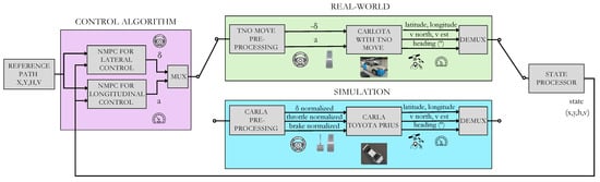
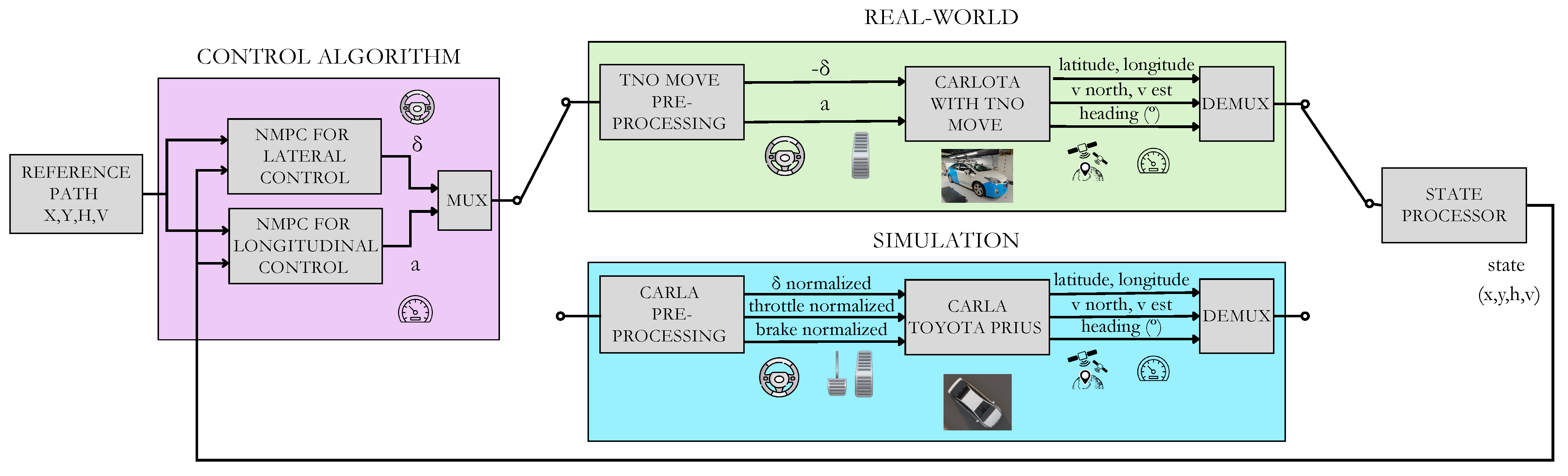
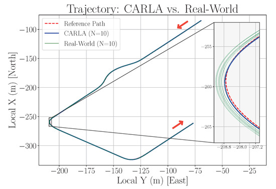
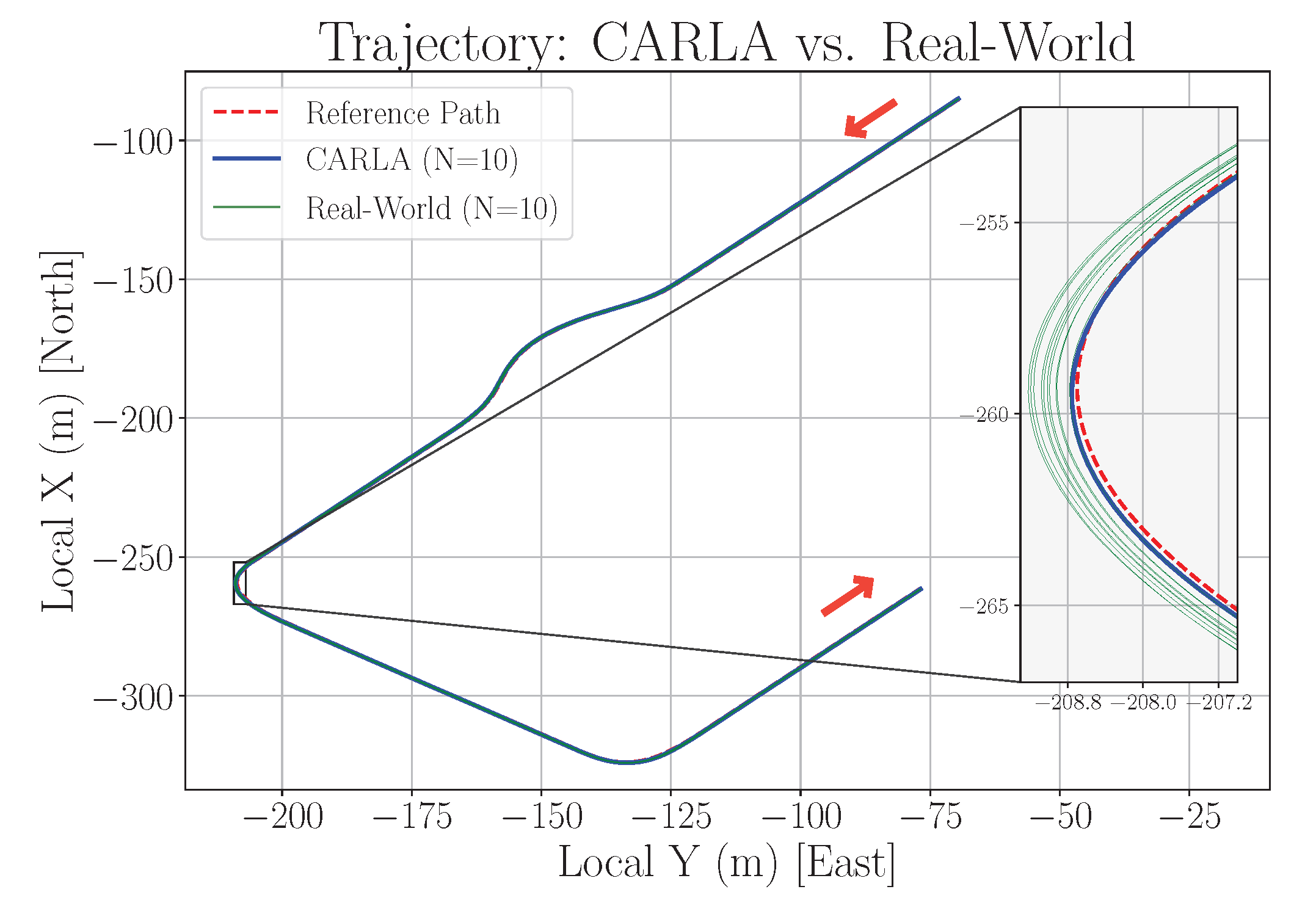
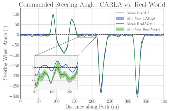
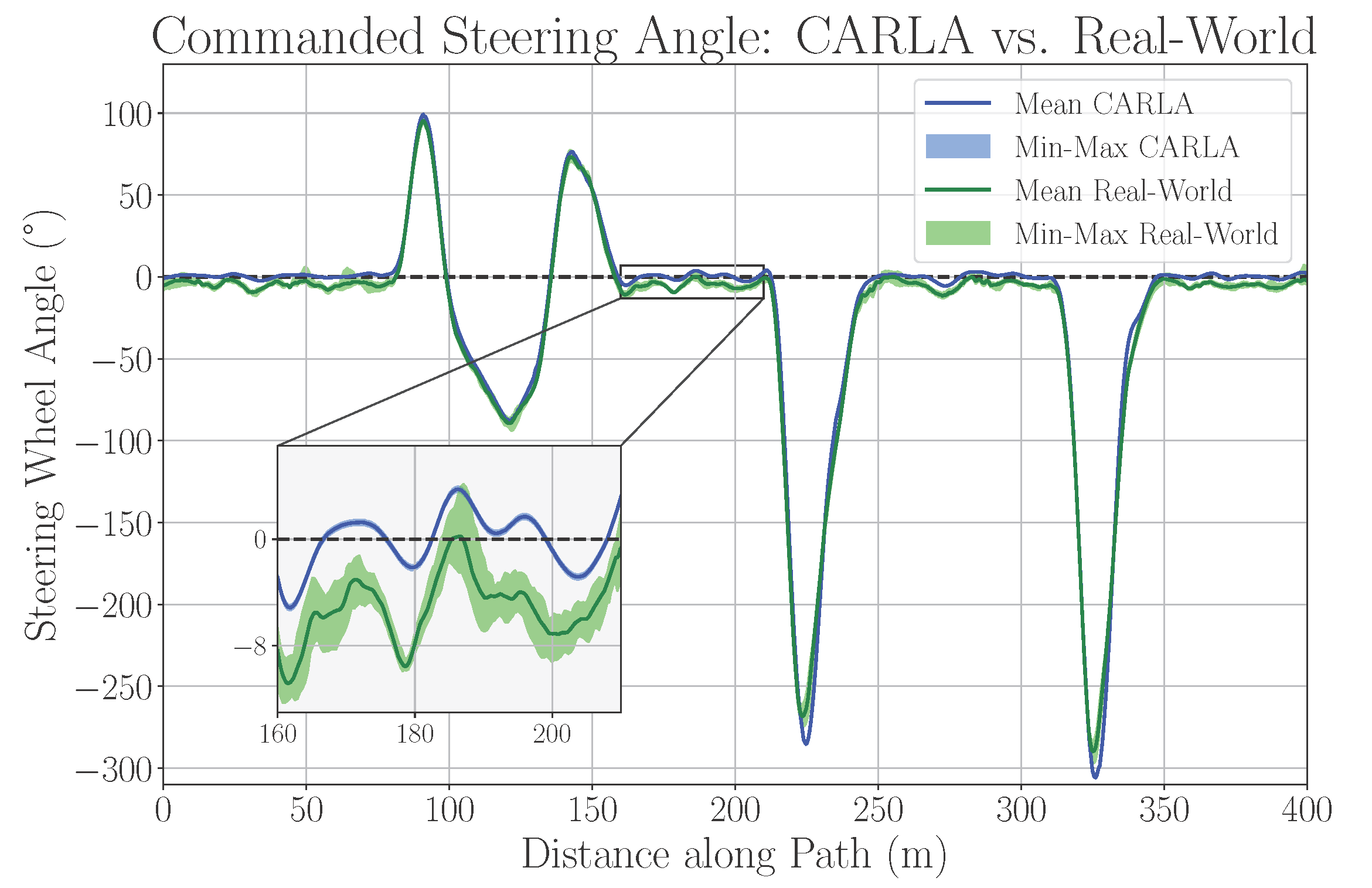
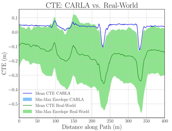
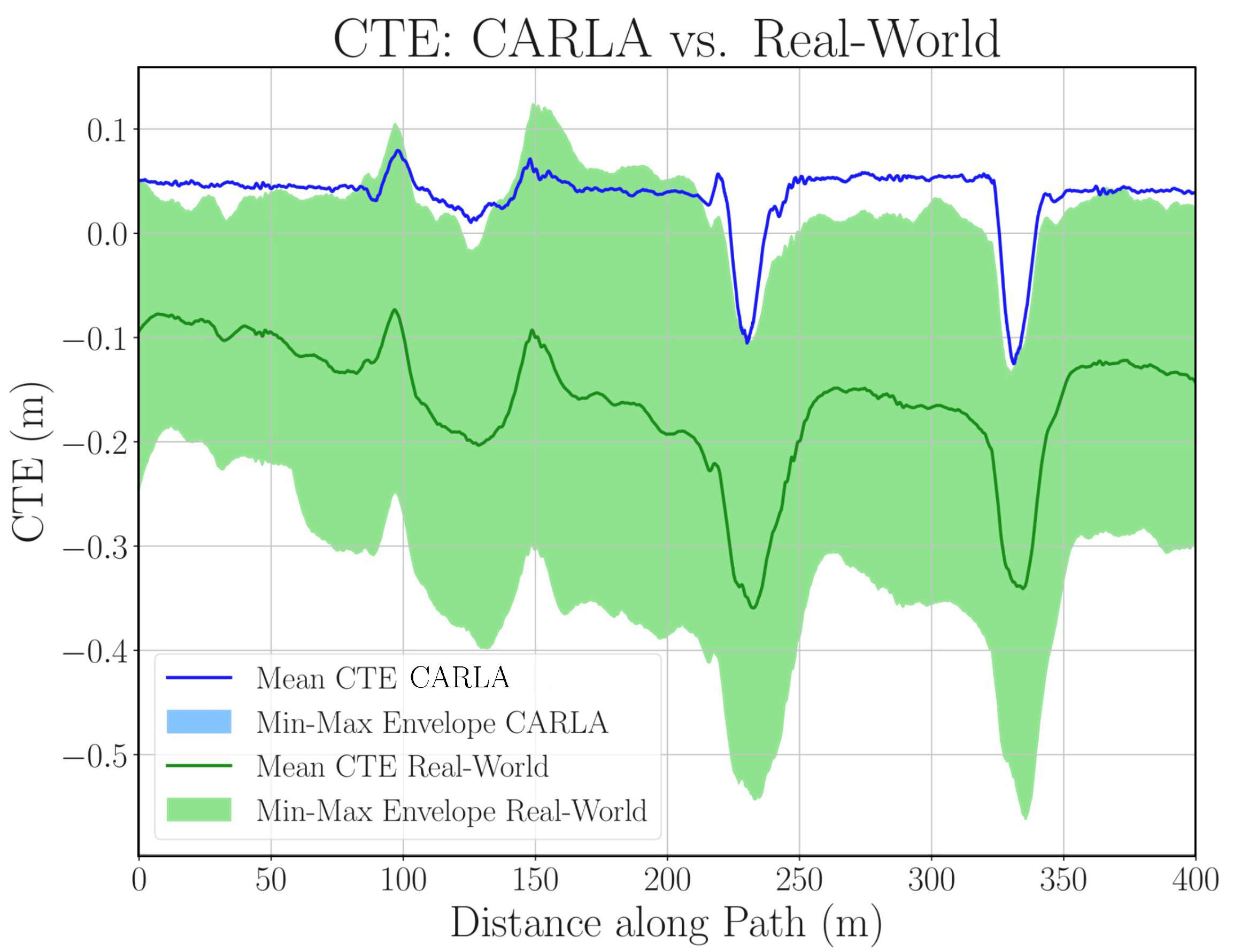
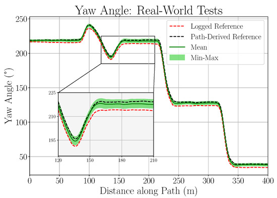
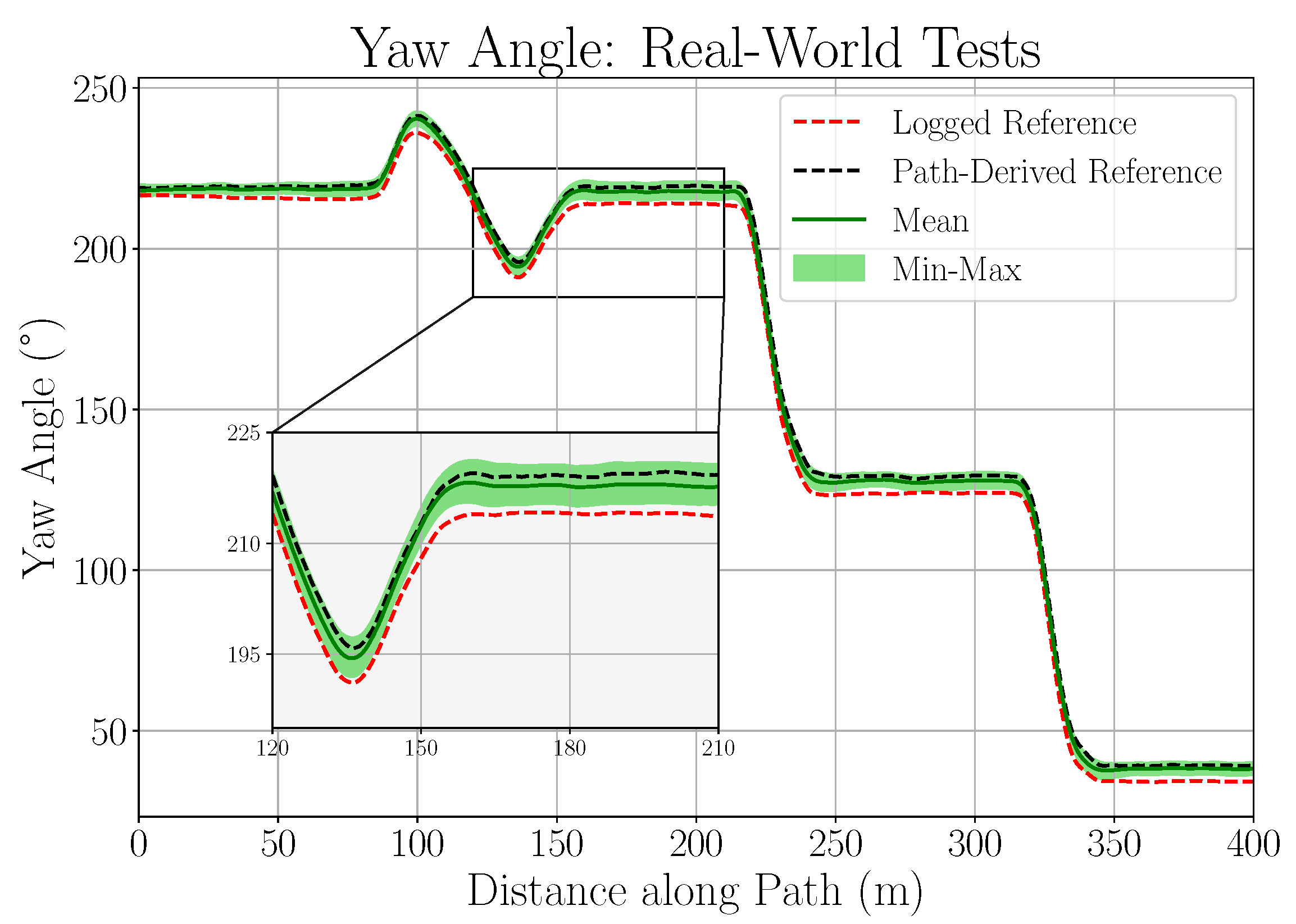
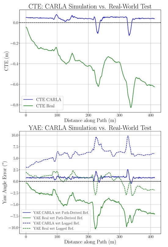
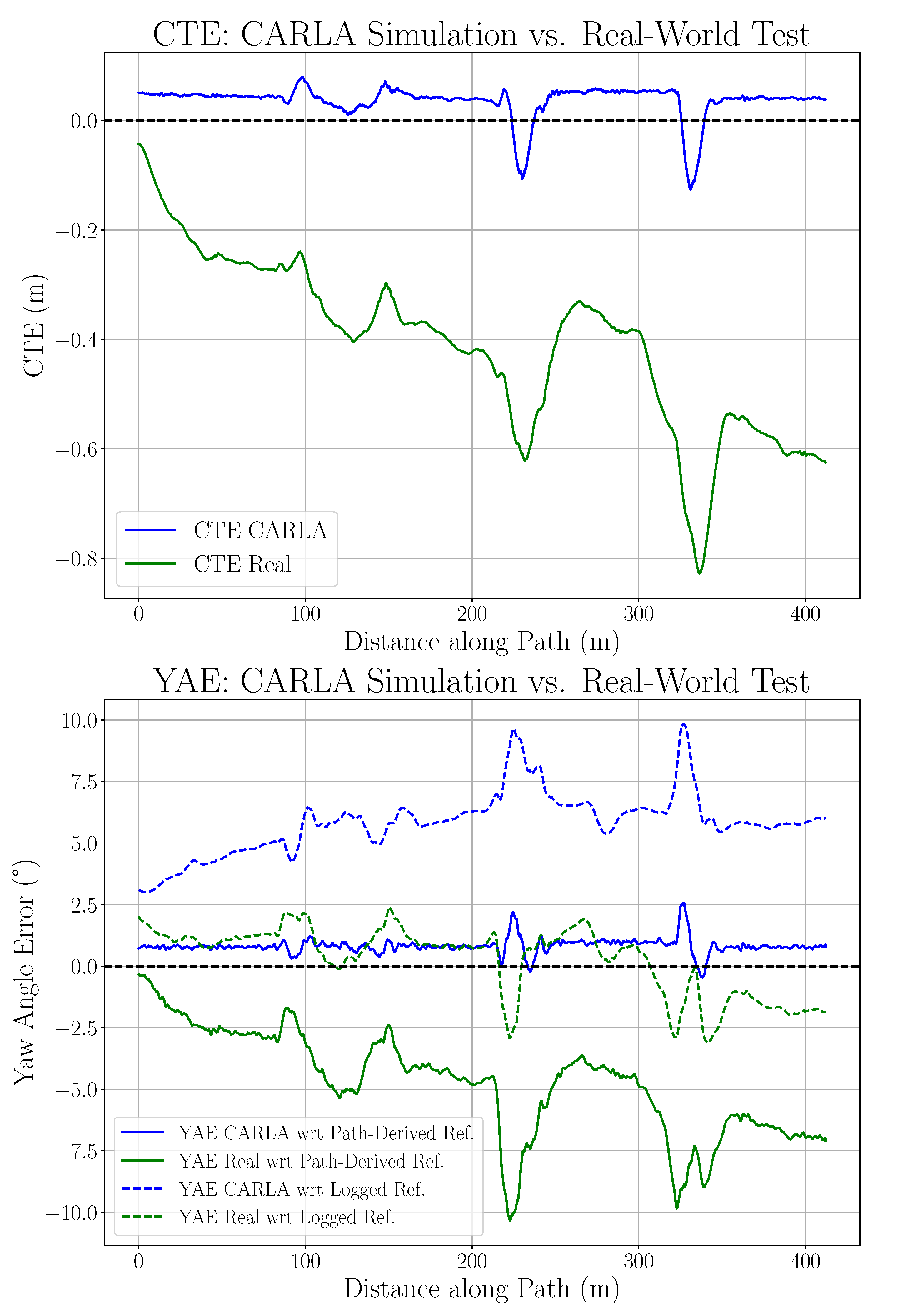
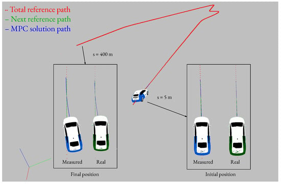
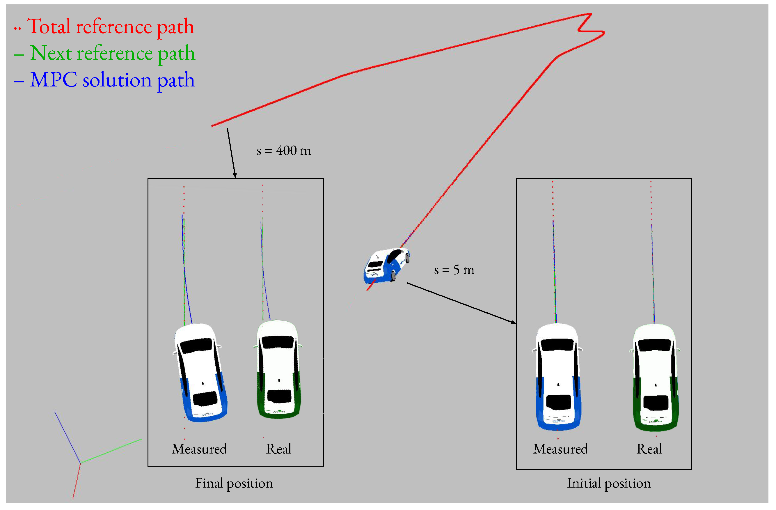
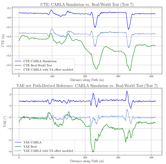
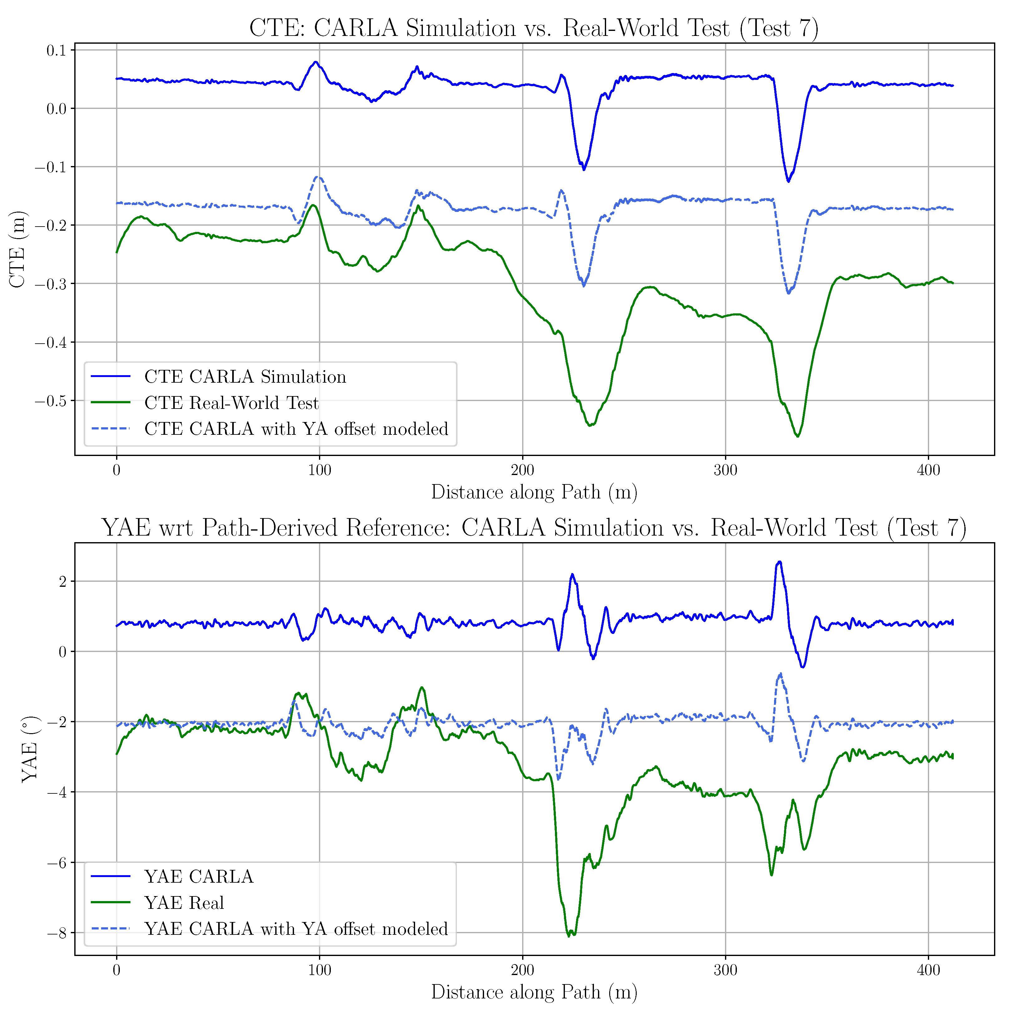
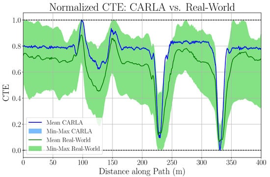
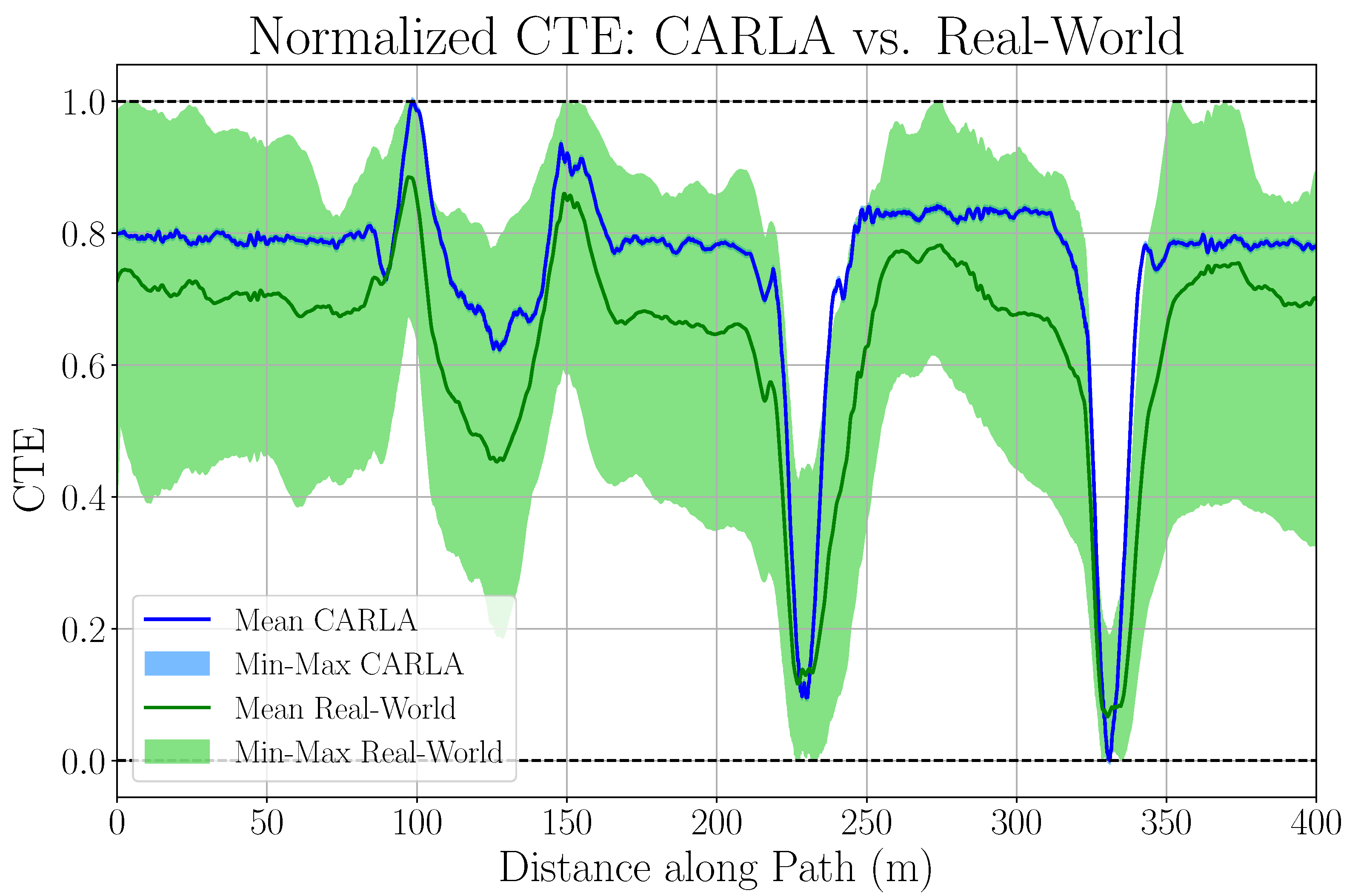
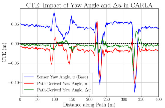
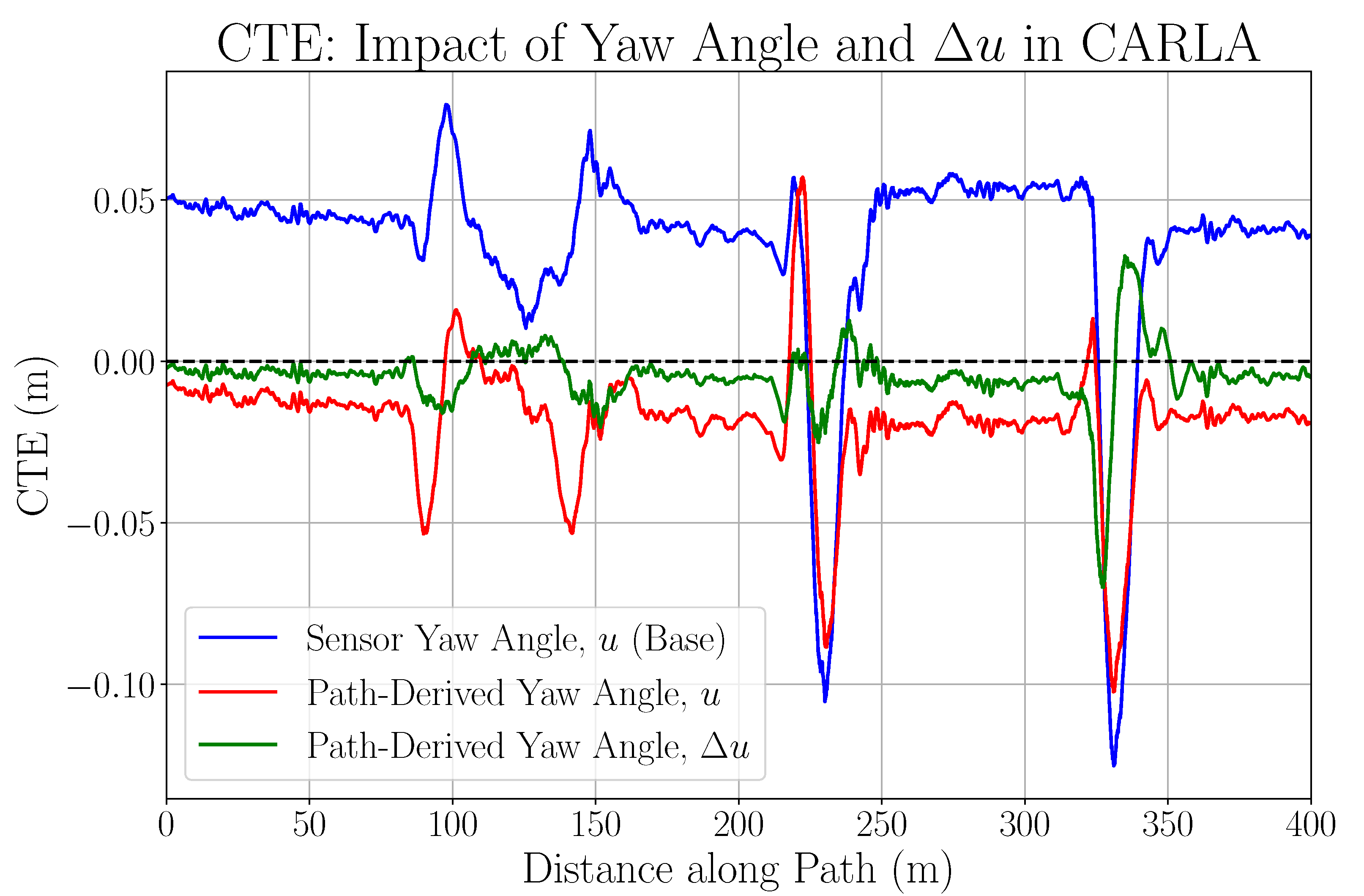
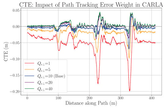
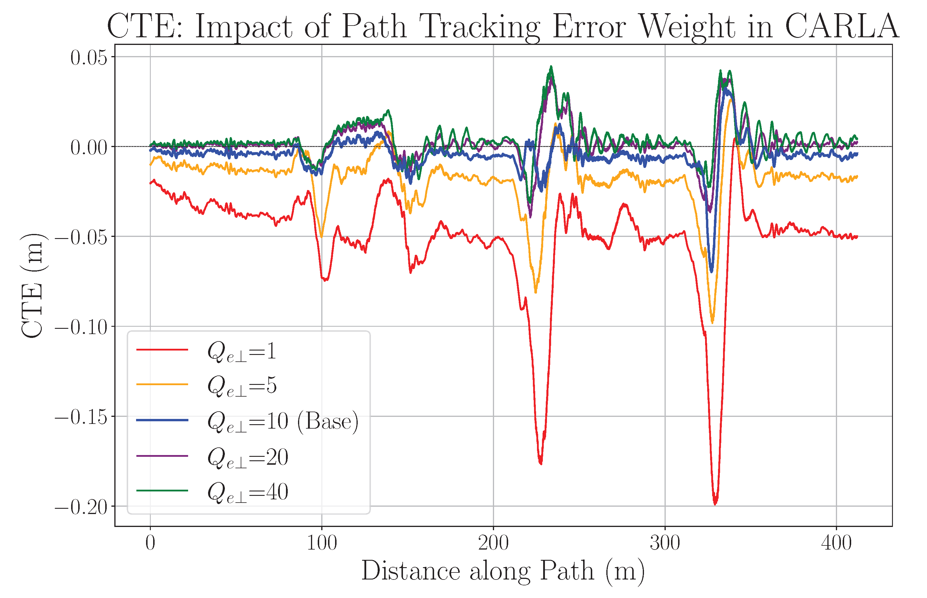
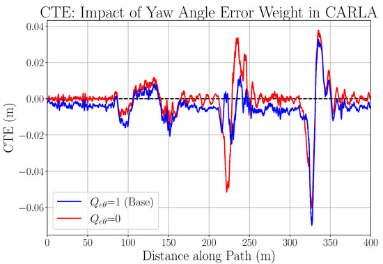
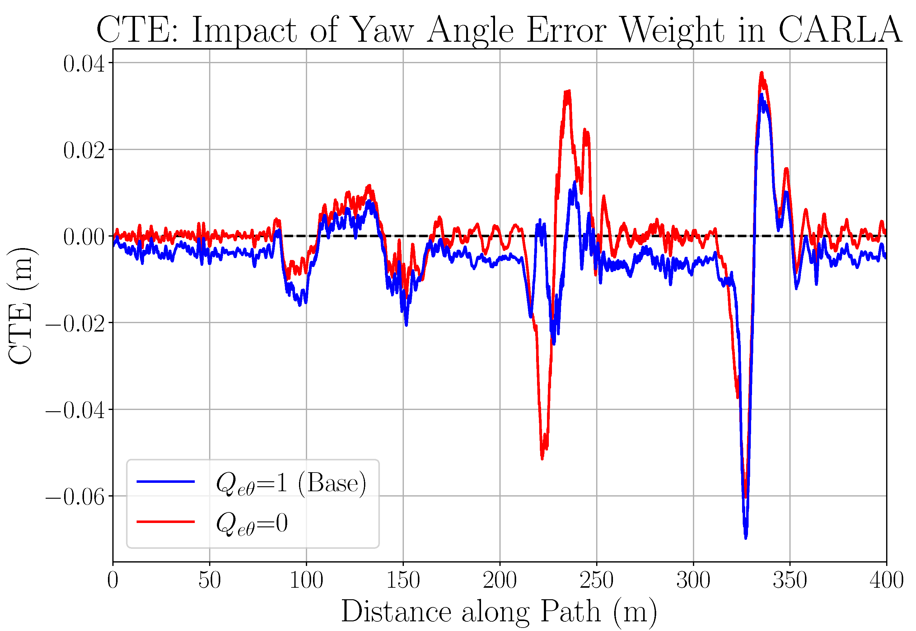
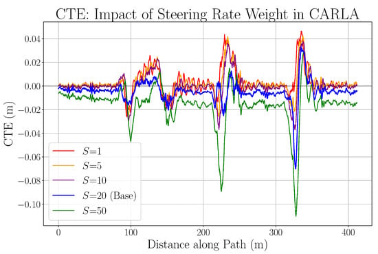
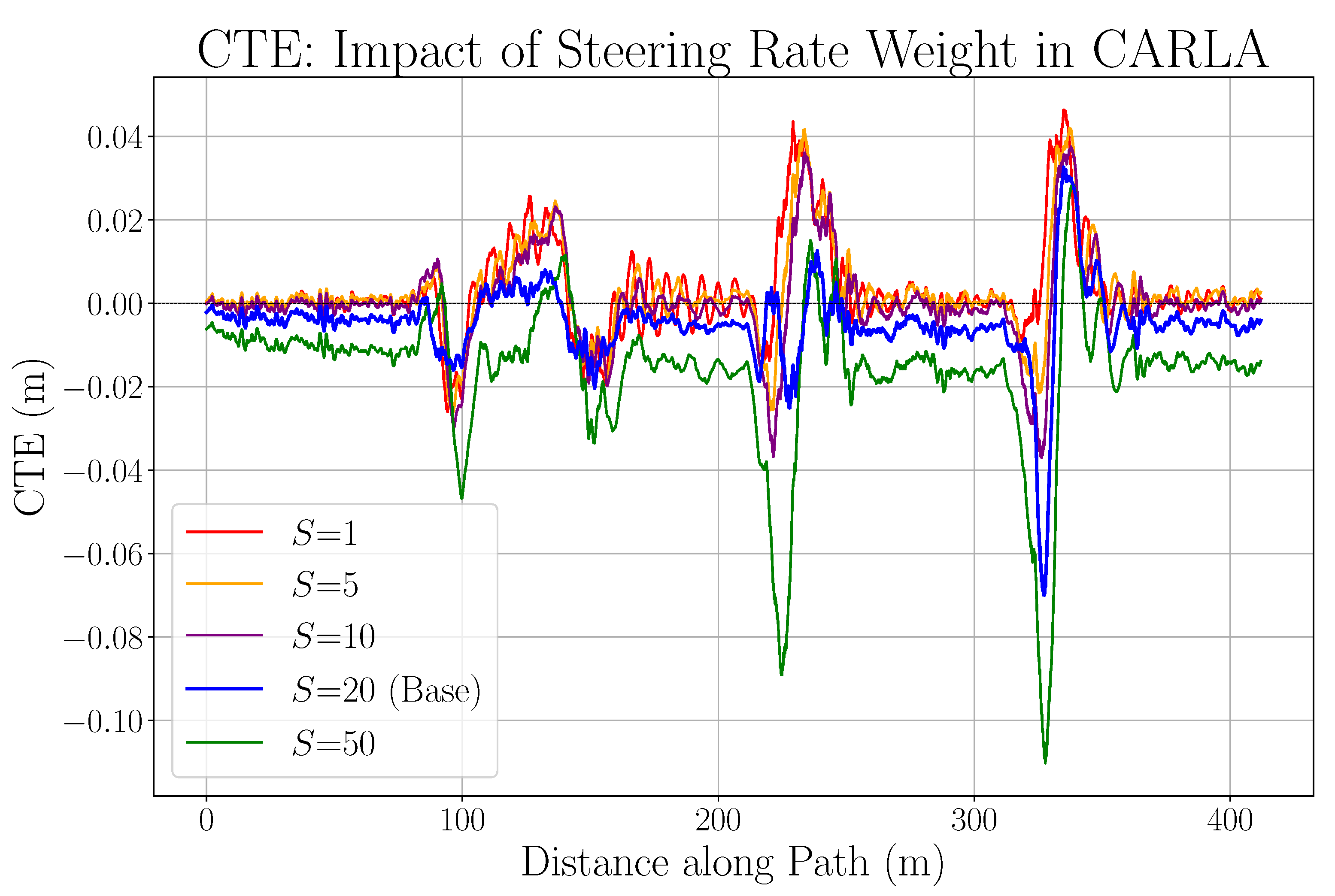

Disclaimer/Publisher’s Note: The statements, opinions and data contained in all publications are solely those of the individual author(s) and contributor(s) and not of MDPI and/or the editor(s). MDPI and/or the editor(s) disclaim responsibility for any injury to people or property resulting from any ideas, methods, instructions or products referred to in the content. |
© 2026 by the authors. Licensee MDPI, Basel, Switzerland. This article is an open access article distributed under the terms and conditions of the Creative Commons Attribution (CC BY) license.