


Abstract
Continuous-variable quantum communication (CVQC) relies on finite-window estimation of phase space moments, making receiver decisions sensitive to finite measurement resolution, calibration uncertainty, and confidence-calibrated tolerances. This paper develops a receiver-centric threat modeling framework for structured (including adversarial) physical-layer disturbances under finite-sample inference. We introduce an operational taxonomy, reconnaissance, exploratory, and denial-of-service, defined by statistical visibility relative to acceptance regions rather than by assumed physical mechanisms. Using an effective estimator space Gaussian model with additive covariance N, we show how distinct mechanisms can be observationally equivalent within finite tolerances and we propose a protocol-agnostic scalar severity coordinate based on the covariance trace. We derive -based missed-detection expressions and a soft detectability boundary scaling as , and we corroborate the predicted behavior via Monte Carlo simulations across representative block sizes. The resulting framework clarifies the delimitation from conventional CV-QKD excess noise parameterization and provides a structured basis for monitoring-layer design and comparative threat-taxonomy mapping.
Keywords:
continuous-variable quantum communication (CVQC); receiver-centric monitoring; physical-layer disturbances; adversarial disturbances; operational threat modeling; acceptance regions; finite-size (finite-sample) effects; missed-detection probability; energy-deviation metric (ΔE); Monte Carlo validation 1. Introduction
Recent advances in quantum communication have made it increasingly clear that security and integrity are shaped not only by idealized theoretical guarantees, but also by operational constraints such as finite measurement resolution, estimator tolerances, and hardware-imposed control limits. In particular, our prior work demonstrated that finite-resolution measurements can induce regions of operational indistinguishability, termed convergence vicinities, in which distinct physical models become experimentally indistinguishable without violating Bell’s theorem itself [1]. That analysis exposed a class of implementation-level vulnerabilities in integrity verification frameworks that rely on static thresholds or idealized measurement assumptions. We emphasize that [1] treats discrete-variable integrity verification under finite-resolution indistinguishability, whereas the present manuscript develops a continuous-variable, receiver-observable threat modeling framework for CVQC based on covariance-level monitoring, regime taxonomy, and finite-sample visibility. The shared element is the receiver-centric tolerance/indistinguishability viewpoint, while the technical setting and observables differ (discrete outcomes vs. covariance-level monitoring).
The present work extends this operational perspective to continuous-variable quantum communication (CVQC), where receiver decisions are driven directly by finite-resolution estimates of phase space statistics. Unlike discrete-variable integrity checks, CVQC systems infer performance- and (when applicable) security-relevant parameters from continuous-valued estimators, quadrature variances, covariances, and covariance matrices, that are intrinsically subject to finite-sample uncertainty and confidence-region design.
In CVQC, quantum information is encoded in the canonical quadratures of optical modes and accessed experimentally via homodyne or heterodyne detection. Rather than treating noise exclusively as an uncontrolled environmental process, we consider adversarial disturbances: intentional, structured perturbations designed to exploit estimator tolerances, probe stability margins, or disrupt communication. For clarity and to reduce repetition, terminology is consolidated in Table 1. Such interference need not appear as anomalously large fluctuations; it can be engineered to remain within nominal operating margins over typical monitoring windows while gradually biasing parameter estimation, degrading coherence, or undermining operational assumptions.
Table 1.
Terminology used in this manuscript.
CVQC plays a central role in quantum communication and networking due to its compatibility with existing optical infrastructure and its scalability [2,3,4]. At the same time, practical CVQC implementations are sensitive to excess noise, phase instability, and detector limitations, which can compromise inferred channel parameters and communication reliability, especially under finite-size parameter estimation constraints [5,6,7,8,9,10,11,12]. These sensitivities define a physical-layer threat surface in which disturbances can be shaped to interact with acceptance criteria and estimator uncertainty [13,14,15,16].
In this work, we classify adversarial interference in CVQC into three operational regimes. Reconnaissance disturbances are low-amplitude perturbations engineered to remain within estimator tolerances while extracting information about system parameters. Exploratory disturbances introduce moderate, structured perturbations intended to probe stability margins and reveal directional sensitivities in phase space. Finally, denial-of-service (DoS) disturbances correspond to high-intensity interference that overwhelms estimation and control capabilities, forcing operational failure. Throughout this work, covariance matrices are expressed in shot-noise units (vacuum variance normalized to unity), and proportionality constants relating energy and covariance trace are omitted for clarity.
To analyze these regimes in an implementation-relevant manner, we adopt a receiver-centric modeling perspective based on an effective Gaussian channel description acting on phase space quadratures. Within this framework, we characterize how disturbances perturb second-order moments accessible to the receiver and how such perturbations translate into estimator degradation and operational failure risk under finite-sample constraints. We introduce an energy deviation metric derived from the covariance trace, providing a compact scalar observable that links disturbance-driven covariance inflation to tolerance design and failure thresholds. Figure 1 provides a receiver-centric schematic of the operational threat surface and the effective estimator-space interpretation of used throughout this work.
Figure 1.
Receiver-centric operational threat surface for continuous-variable quantum communication. Schematic diagram (not to scale): Arrows indicate conceptual points of adversarial influence (e.g., phase reference manipulation, injected disturbances/jamming, detector/ADC saturation), while receiver decision logic is based on finite-resolution estimators of first- and second-order quadrature moments (mean/covariance). The pair denotes the total observable effect inferred at the receiver and need not coincide with the adversary’s physical mechanism or implementation. The diagram provides an operational interpretation of the effective Gaussian channel model in Equation (1), not a specific hardware layout. Simulation-based missed-detection curves are provided later (Section 3.8) to complement the schematic regime illustrations.
This manuscript focuses on receiver-observable operational threat modeling. It provides a regime taxonomy and observable-level characterization of adversarial interference, but it does not constitute a protocol security proof, a mitigation design, or a prescriptive detection mechanism. In particular, the mapping from a physical disturbance to inferred effective parameters in Equation (1) (Section 3) is generally non-identifiable without additional instrumentation or assumptions because distinct mechanisms can induce statistically indistinguishable changes in finite-sample covariance estimates. The regimes defined here should therefore be interpreted as operational equivalence classes in estimator space. We also discuss the consequences of allowing estimator space G that is not constrained to be physically realizable and how physical plausibility constraints can be imposed when desired (Section 3).
Specifically, this work makes three contributions: (i) it formalizes a taxonomy of adversarial disturbance regimes in CVQC grounded in operational intent and estimator visibility; (ii) it develops a Gaussian channel modeling framework that captures adversarial interference at the level of receiver-accessible covariance statistics without assumptions about adversary capabilities; and (iii) it introduces an energy deviation metric and finite-sample detectability analysis that connect disturbance-driven covariance inflation to estimator tolerances and operational failure boundaries. To complement the analytic visibility bounds, we include Monte Carlo simulation plots that corroborate the predicted missed-detection behavior and its scaling under the stated i.i.d. baseline assumptions (Section 3.8). Together, these results establish a structured, receiver-centric foundation for analyzing physical-layer adversarial behavior in continuous-variable quantum communication.
Remark 1
(Normalization convention used throughout). Unless stated otherwise, we use shot-noise unit (SNU) normalization in which the vacuum variance is unity, i.e., for a single mode (and for m modes ). All covariance matrices, tolerances, and energy deviation quantities in this paper are expressed relative to this convention.
2. Related Work and Gap Statement
2.1. Continuous-Variable Quantum Communication and Parameter Estimation
Continuous-variable quantum communication (CVQC) protocols encode information in the amplitude and phase quadratures of optical modes and rely on statistical inference over continuous measurement outcomes to establish correctness, performance, and, where applicable, security. Homodyne and heterodyne detection provide direct access to quadrature observables, making CVQC naturally compatible with Gaussian state modeling and covariance matrix descriptions [2,4].
A central component of CVQC operation is parameter estimation. Practical implementations infer quantities such as channel loss/transmittance, excess noise, quadrature variances, and covariance structure from finite ensembles of measurement outcomes. These estimates drive operational decisions, including acceptance/abort conditions in quantum key distribution, calibration and stability assessment in quantum networking, and performance evaluation in sensing and verification tasks [2,7,9,17,18]. Consequently, CVQC reliability depends critically on the finite-sample behavior of these estimators, especially in regimes where confidence regions and acceptance thresholds must be defined explicitly [5,6,7].
Most existing analyses of CVQC parameter estimation emphasize environmental and device-induced noise sources, including thermal noise, detector inefficiency, phase drift, and loss [4,8,13]. Within this prevailing treatment, excess noise is typically modeled as stationary (or slowly time-varying) stochastic variability, and performance/security conclusions are derived under assumptions of well-characterized noise statistics and asymptotic or large-sample limits.
However, in deployment settings, parameter estimation is constrained by finite measurement resolution, finite-sample sizes, and implementation-specific acceptance margins. These constraints induce estimator tolerances: bounded regions in parameter space within which observed statistics are deemed consistent with nominal operation. While necessary for robust operation, tolerances also create operational indistinguishability regions in which distinct underlying disturbances produce statistically indistinguishable receiver observations over finite monitoring windows.
Recent work in discrete-variable quantum integrity verification has shown that finite-resolution effects can be systematically exploited by adversarial probing strategies that remain within estimator tolerances while biasing inferred parameters [1]. In continuous-variable systems, where decisions are made directly from continuous-valued estimators, analogous vulnerabilities can arise in covariance/phase space statistics. Nevertheless, the CVQC literature has largely treated parameter estimation as a passive inference component rather than as a receiver-side decision surface that can be shaped or exploited by structured disturbances interacting with tolerance design.
Beyond “benign” noise models, growing security implementation literature documents receiver interface and calibration-sensitive attacks that can manipulate or distort measured statistics without necessarily presenting as gross anomalies. In CV-QKD, examples include attacks that exploit detector non-idealities (e.g., saturation and blinding-type behaviors) and attacks that target calibration and wavelength-dependent components, with consequences that can appear as biased or inflated covariance estimates from the receiver’s perspective [13,14,15,16]. These results motivate treating monitored estimators and their acceptance regions as part of the operational attack surface, especially under finite-size parameter estimation constraints and composable security settings where confidence intervals must be handled explicitly [6].
This gap motivates a receiver-centric, operational examination of parameter estimation in CVQC under adversarial conditions. Rather than assuming noise to be purely environmental or benign, the present work analyzes how structured disturbances interact with finite-resolution/finite-sample estimation and how their impact manifests in experimentally accessible covariance statistics. This perspective reframes parameter estimation not only as a tool for system characterization, but also as a potential locus of adversarial exploitation in continuous-variable quantum communication.
2.2. Threat Modeling Frameworks and Quantum-Specific Taxonomies
Classical cybersecurity threat modeling frameworks provide systematic languages for describing adversarial intent, tactics, and operational pathways. STRIDE-style approaches organize threats around system properties (e.g., spoofing, tampering, and denial-of-service), while MITRE ATT&CK-style approaches emphasize tactic/technique/procedure taxonomies that support adversary emulation and detection engineering [19]. These frameworks are not quantum-specific, but they motivate the value of structured, implementation-aware threat descriptions that are separable from any single device configuration.
Recent work has begun to develop analogous taxonomies for quantum communication systems. In particular, the SQOUT framework [20] proposes a threat analysis methodology for quantum communication systems inspired by MITRE ATT&CK principles and kill-chain models, with the goal of bridging quantum-domain threats to classical cybersecurity practice. SQOUT is therefore directly relevant to positioning receiver-centric CVQC threat modeling within the broader landscape of cybersecurity-oriented taxonomies. Table 2 compares representative security/threat frameworks relevant to CVQC monitoring and threat modeling.
Table 2.
Structured comparison of security/threat frameworks relevant to CVQC monitoring and threat modeling.
Table 3 shows where the present work sits relative to those existing frameworks.
Table 3.
Where the present work sits relative to existing frameworks.
2.3. Implementation Constraints: Finite-Resolution, Finite Samples, and Acceptance Regions
Practical continuous-variable quantum communication (CVQC) systems operate under unavoidable implementation constraints that shape how quantum states and channels are characterized in practice. Chief among these constraints are finite measurement resolution, finite-sample sizes, and the use of predefined acceptance regions for parameter estimation. Together, these factors determine the operational limits of inference and play a central role in how noise, benign or adversarial, manifests in experimentally accessible statistics. Because acceptance decisions are made from finite-window estimates, these same constraints also define the receiver’s monitoring-layer and the statistical “decision surface” that an adversary can attempt to probe or exploit.
Finite measurement resolution arises from detector noise, electronic bandwidth limitations, digitization, and coarse-graining of continuous outcomes. Homodyne and heterodyne measurements therefore yield discretized quadrature samples with nonzero uncertainty, even under idealized state preparation. As a result, small perturbations to underlying quadrature distributions may be indistinguishable from measurement-induced fluctuations, particularly over limited observation windows [4,8,9].
Finite-sample sizes further constrain parameter estimation. In operational settings, covariance matrices and excess noise parameters are inferred from a limited number of measurement outcomes, leading to statistical uncertainty that scales inversely with the number of samples. Confidence intervals and hypothesis tests used in protocol verification must therefore accommodate estimator variance, introducing tolerance margins that grow as sample sizes decrease or noise levels increase. These finite-size effects and confidence-region constructions are well established in continuous-variable quantum key distribution and related CV platforms [5,6,21]. These effects are well understood in benign noise models but become critical when disturbances are structured or non-stationary. Importantly, the underlying variance estimation and confidence-region behavior is classical and standard; the gap for CVQC threat modeling is not the statistics themselves, but how tolerance regions and finite-n visibility shape operational indistinguishability and regime transitions under structured disturbances.
In addition, finite-window inference commonly faces temporal correlations induced by phase reference dynamics, drift, and feedback/control loops. In such cases, the nominal window size n can overstate statistical resolution, and an effective sample size provides a more realistic proxy for estimator uncertainty. This motivates explicitly tracking correlation-aware monitoring performance (e.g., via ) when interpreting detectability boundaries in Section 3.8.
To ensure reliable operation, CVQC implementations define acceptance regions for estimated parameters, within which observed statistics are deemed consistent with nominal behavior. These regions may be specified explicitly, as in security margins for quantum key distribution, or implicitly, through calibration thresholds and performance criteria in communication and networking applications. Acceptance regions are thus an integral part of system design, translating statistical uncertainty into operational decision rules. From an operational monitoring perspective, acceptance regions play the same role as thresholds in change detection and statistical process monitoring: they convert noisy estimates into actionable decisions and alarms over time [22,23].
While acceptance regions are necessary for practical operation, they also define regions of operational indistinguishability. Distinct physical disturbances that induce parameter shifts smaller than estimator tolerances cannot be reliably discriminated by the receiver, even if they are systematic or adversarial in origin. This phenomenon has been identified in discrete-variable integrity verification as a source of exploitable structure under finite-resolution measurements. In continuous-variable systems, where decisions are made directly from continuous-valued estimators, analogous indistinguishability arises naturally from finite-resolution and finite data.
Existing CVQC analyses typically treat these implementation constraints as technical limitations to be mitigated through longer integration times or improved hardware. In contrast, the present work treats finite-resolution, finite samples, and acceptance regions as defining features of the operational threat landscape. By explicitly incorporating these constraints into the characterization of adversarial interference, we expose how estimator tolerances shape the boundary between detectable and operationally invisible disturbances in continuous-variable quantum communication. This perspective also motivates including explicit simulation-based illustrations of missed-detection behavior versus disturbance strength and sample size, which we provide in Section 3.8 to validate the finite-n visibility mechanism under the stated baseline assumptions.
2.4. Physical-Layer Adversaries in Optical/CV Links: Excess Noise, Phase Perturbations, and Jamming
Physical-layer adversaries targeting optical and continuous-variable (CV) communication links have been studied primarily through the lenses of excess noise, phase instability, and optical jamming. In much of the existing literature, such disturbances are treated as environmental or technical imperfections, including thermal noise, laser phase noise, imperfect synchronization, and channel loss fluctuations. These effects are typically assumed to be stationary or weakly time varying, and mitigation strategies focus on calibration, stabilization, and post-processing [2,4].
Excess noise is a central performance-limiting factor in CVQC, particularly in continuous-variable quantum key distribution (CV-QKD), where security thresholds are formulated in terms of tolerable noise above the shot-noise limit [24]. Prior work has extensively analyzed how excess noise degrades key rates, limits transmission distance, and constrains security margins. However, excess noise is most often treated as an aggregate parameter arising from uncontrolled environmental processes or imperfect components, rather than as a deliberately structured disturbance shaped to interact with estimator tolerances or to bias receiver-side calibration and parameter inference within acceptance regions.
Phase perturbations constitute another well-studied class of physical-layer effects in optical links. Phase noise can arise from laser linewidth, fiber fluctuations, or reference-frame misalignment, and has motivated substantial work on phase tracking, compensation, and synchronization [25]. These studies typically assume benign drift or stochastic fluctuations and aim to maintain a stable phase reference. Intentional phase perturbations that are structured in time (or biased in sign) to probe directional sensitivities or estimator robustness are less commonly addressed explicitly, despite the fact that many operational decisions in CV receivers are based on finite-window covariance estimates.
Optical jamming and denial-of-service-like interference have also been considered in classical and quantum optical communication, particularly in free-space or shared-fiber scenarios [13]. In quantum settings, such interference is often associated with overt disruption, detector saturation, or protocol abort conditions. As a result, jamming is frequently treated as an easily detectable failure mode rather than as part of a continuum of adversarial behavior that includes stealthy or sub-threshold disturbances that remain statistically consistent with nominal operation over typical monitoring windows.
A growing body of work further highlights that optical and CV quantum links are susceptible to implementation-level attacks, including detector saturation, local oscillator (LO) manipulation, wavelength-dependent attacks, and calibration-dependent exploits that bypass idealized security assumptions while remaining compatible with nominal parameter estimates [7,13,14,15,16,26]. These studies emphasize that adversarial control over physical-layer degrees of freedom can translate into estimator bias, parameter mischaracterization, or forced protocol behavior without violating abstract protocol models; in many cases, the observable impact can be absorbed into receiver-inferred effective parameters rather than appearing as a single “obvious” anomaly. From an operational monitoring viewpoint, these implementation attacks motivate explicitly tying attack impact to receiver-side acceptance tests and monitoring thresholds, i.e., to what is visible in finite-window estimates of (and derived scalars such as Tr()) rather than to an assumed unique physical mechanism.
Across these bodies of work, a common implicit dichotomy is that physical-layer disturbances are either benign noise to be estimated and compensated, or catastrophic interference that immediately invalidates operation. This dichotomy obscures intermediate regimes in which disturbances are intentionally shaped to remain within accepted operating margins while extracting information, biasing inference, or mapping system robustness. Moreover, prior analyses seldom connect physical-layer perturbations directly to the estimator tolerances and acceptance regions that govern operational decisions at the receiver (e.g., confidence-calibrated acceptance tests on or on excess noise surrogates).
The present work departs from this perspective by treating excess noise, phase perturbations, and jamming as manifestations of a broader class of adversarial interference at the physical layer. Rather than classifying disturbances solely by physical mechanism, we organize them by operational intent and by their impact on receiver-side observables relative to estimator tolerances. This receiver-centric viewpoint enables a unified treatment of stealthy probing, stress-inducing perturbations, and overt disruption within a single operational threat modeling framework for continuous-variable quantum communication at the level of receiver-estimated first/second moments. To complement the schematic regime figures, Section 3.8 includes simulation-based plots (Monte Carlo overlays) of versus for multiple n, which validate the finite-n visibility mechanism used to separate reconnaissance from exploration under the stated baseline assumptions.
To situate the proposed regime taxonomy within the broader landscape of physical-layer security research, it is useful to relate the operational regimes defined here to representative families of implementation-level interference studied in optical and CV systems. This mapping is not intended to propose, analyze, or validate specific attack implementations. Rather, it provides an interpretive bridge between mechanism-agnostic adversarial regimes, defined by receiver-observable impact relative to estimator tolerances, and representative families of physical-layer interference discussed in the literature.
The associations in Table 4 should be interpreted strictly at the level of receiver-observable effects. Multiple physical mechanisms may map to the same effective disturbance in estimator space, and a single physical-layer technique may realize different operational regimes depending on amplitude, timing, and interaction with finite-sample tolerances. Therefore, regime classification in this work is determined by statistical visibility and operational consequence at the receiver, not by assumptions about attacker hardware, access, or intent. Figure 2 summarizes the operational regime ladder that underlies the attack-family interpretation in Table 4.
Table 4.
Mechanism-agnostic adversarial regimes mapped to representative physical-layer attack families in optical/CV links. The mapping is receiver-centric and illustrative: it links each family to its dominant observable effect (effective in Equation (1)) and to the operational regime taxonomy, without assuming specific adversary implementations. Representative discussions of these attack families can be found in [7,8,13,14,15,16]. The same physical family may map to different regimes depending on amplitude, timing, and windowing.
Figure 2.
Adversarial regime ladder versus tolerance ratio and receiver-observable signatures. Schematic (not to scale): The “acceptance boundary” denotes the boundary of a receiver-defined acceptance region in estimator space, and the “failure threshold” denotes an operational abort/failure limit (hardware or protocol). Regimes are distinguished operationally by disturbance magnitude relative to estimator tolerances (e.g., ), transitioning from acceptance-region stealth (reconnaissance) to measurable stress (exploratory) and ultimately to failure beyond operational thresholds (DoS). This schematic ladder is complemented by simulation-based missed-detection curves versus for multiple n in Section 3.8, which corroborate the finite-n visibility mechanism used to separate reconnaissance from exploration under the stated baseline assumptions.
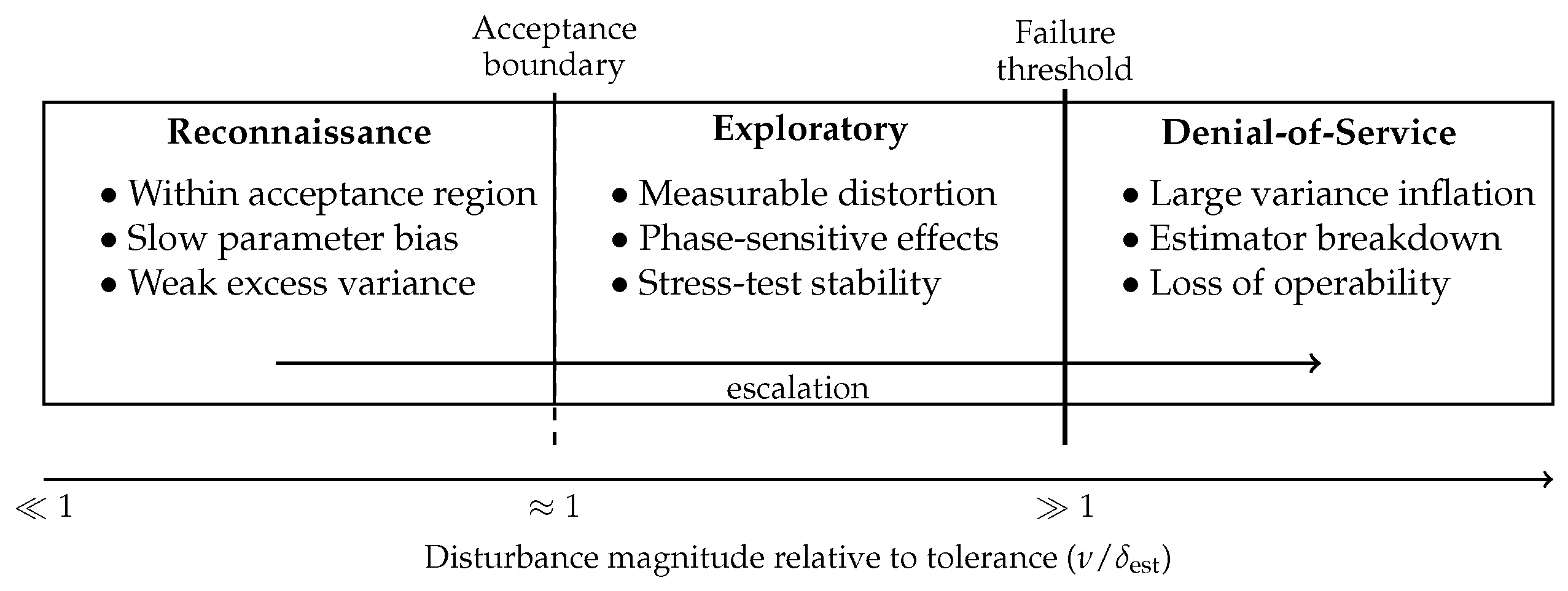
Figure 3.
Phase space covariance ellipses (Wigner-like contours) illustrating how operational regimes manifest in receiver-accessible second-order statistics. Schematic ellipses (illustrative, not experimental data): Reconnaissance disturbances remain within the receiver-defined energy deviation tolerance (i.e., ) over a monitoring window; exploratory disturbances introduce anisotropic distortion and/or phase space rotation, with near a detectability boundary (noting that , being trace-based, is rotation-invariant and therefore does not by itself detect pure rotational attacks); DoS disturbances yield large variance inflation with , consistent with estimator breakdown and operational failure. This conceptual phase space illustration is complemented by simulation-based missed-detection curves versus for multiple window lengths n in Section 3.8, which provide data-driven corroboration of the finite-n visibility mechanism used in the regime boundary discussion.
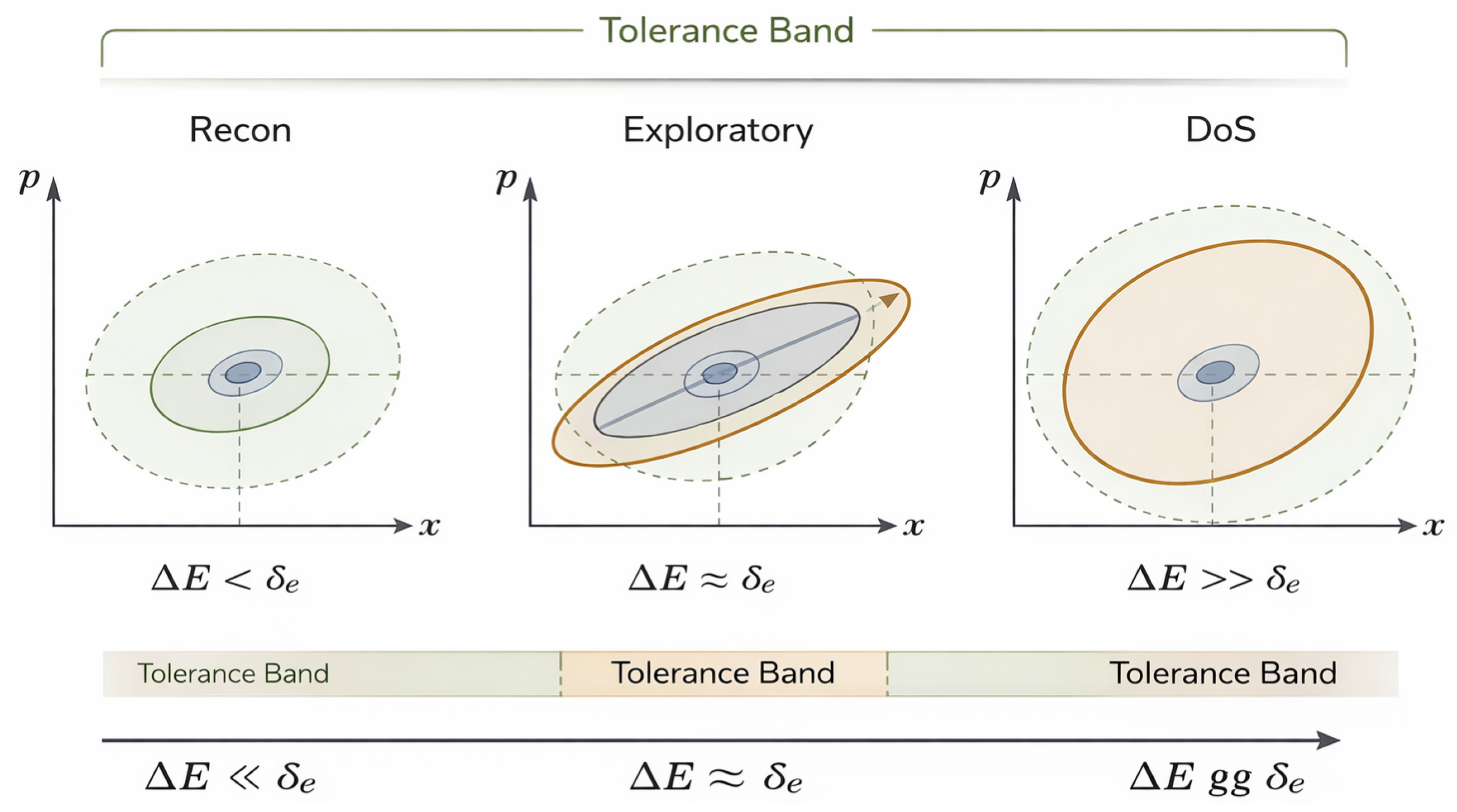
Figure 4.
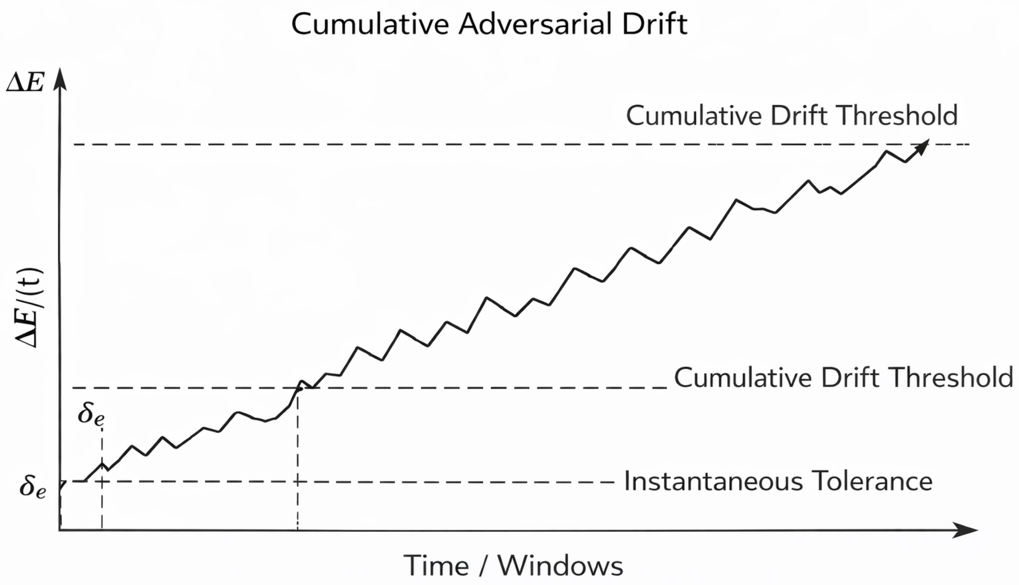
Illustration of cumulative adversarial drift under repeated sub-threshold perturbations. Schematic time series (illustrative): Each monitoring window remains within an instantaneous acceptance tolerance (dashed line at ), so short-term tests may raise no alarm; however, the accumulated energy deviation can drift upward across windows and eventually exceed a long-horizon drift threshold, indicating delayed detectability and/or parameter bias despite per-window acceptance. This delayed detectability effect is directly analogous to finite-size CV-QKD parameter estimation behavior, where excess noise can remain statistically consistent with nominal confidence bounds on a per-block basis yet become evident only through longer-horizon monitoring or tighter finite-size confidence accounting [5,6,7]. The paper additionally includes Monte Carlo missed-detection curves versus for multiple n in Section 3.8, which provide data-driven corroboration of the finite-n “stealth band” mechanism that underlies this qualitative drift picture.
2.5. Gap and Contributions
Despite extensive studies on noise, loss, and imperfections in continuous-variable quantum communication (CVQC), a clear gap remains in how physical-layer interference is conceptualized and analyzed from an adversarial perspective. Existing work predominantly treats excess noise, phase instability, and jamming either as benign effects to be estimated and compensated, or as catastrophic failures that immediately invalidate operation. This framing overlooks intermediate regimes in which disturbances are deliberately structured to exploit finite measurement resolution, finite-sample sizes, and estimator tolerances without necessarily triggering protocol aborts or anomaly flags. In particular, finite-window monitoring can admit a tolerance-induced “stealth band” in which structured disturbances remain statistically consistent with nominal operation for typical block sizes.
Relative to our prior work on discrete-variable integrity verification and convergence vicinities [1], the present study extends operational indistinguishability to continuous-variable systems by translating indistinguishability from outcome statistics to covariance/estimator space in CVQC, and by making the receiver’s acceptance regions explicit as decision surfaces that can be probed by an adversary. This clarification also addresses overlap concerns by distinguishing the discrete-variable verification setting in [1] from the present covariance-level CVQC monitoring framework.
Prior analyses rarely formalize how receiver-side acceptance regions and confidence thresholds shape what constitutes an operationally detectable disturbance. As a result, there is limited machinery for reasoning about stealthy probing, gradual parameter biasing, or adversarial stress-testing at the physical layer of CVQC systems in a way that is decoupled from any single device model. Moreover, while security and robustness are often discussed at the protocol or information-theoretic level, there is a lack of receiver-centric threat models that directly connect physical-layer interference to experimentally accessible observables such as covariance matrices and inferred energy, while explicitly acknowledging the non-identifiability of the underlying physical mechanism from finite-sample statistics.
This work addresses these gaps by introducing an explicitly operational threat modeling framework for adversarial disturbances in CVQC. The central contributions are threefold:
- (i)
- Receiver-observable regime taxonomy. We formalize a taxonomy of adversarial disturbance regimes, reconnaissance, exploratory, and denial-of-service, distinguished by operational intent and by observable impact relative to estimator tolerances, rather than by assumed physical mechanisms.
- (ii)
- Estimator space effective model. We develop a Gaussian channel modeling approach that captures adversarial interference at the level of receiver-accessible phase space statistics, treating as an effective receiver-inferred description rather than a unique physical attribution.
- (iii)
- Scalar severity coordinate and finite- visibility. We introduce an energy deviation metric derived from the trace of the covariance matrix and connect it to finite-sample detectability through missed-detection behavior and operational boundaries under explicit acceptance regions.
- Formal delimitation from conventional excess noise parameterization
- We do not claim that Tr-based monitoring or variance estimation is new; these are standard tools in Gaussian-CV modeling and in CV-QKD parameter estimation. The novelty is operational: we (i) use acceptance regions/tolerances as explicit receiver decision surfaces that induce tolerance-defined indistinguishability bands; (ii) organize adversarial behavior into a mechanism-agnostic regime taxonomy (reconnaissance/exploratory/DoS) in terms of estimator visibility; and (iii) connect this taxonomy to finite-n missed-detection behavior that quantifies when disturbances remain operationally hidden. In particular, conventional CV-QKD excess noise models can be recovered as special cases of the estimator space viewpoint when one restricts to physically motivated parameterizations; our scope is broader because we intentionally characterize what is visible to the receiver under finite-resolution and finite-data even when mechanism identification is not possible.
- Validation under the stated baseline assumptions
- To move beyond purely schematic figures, we include Monte Carlo simulation plots that overlay empirical estimates of on the analytic -based prediction for multiple block sizes n (Section 3.8). These simulations validate the finite-n visibility mechanism used to separate reconnaissance from exploration under the i.i.d. Gaussian baseline; they are not presented as device-specific experimental validation.
3. Receiver-Observable Modeling of Adversarial Disturbances
From a cybersecurity perspective, adversarial disturbances in CVQC constitute a physical-layer attack surface: structured perturbations can exploit estimator tolerances, control assumptions, and finite-resolution effects by acting on the receiver’s inference layer and decision margins.
In continuous-variable (CV) quantum systems, quantum information is encoded in the canonical quadratures and of optical modes. These quadratures fully characterize Gaussian quantum states and form the operational foundation of CVQC systems and devices [4]. As a result, performance- and integrity-relevant information in CVQC is inferred from finite-resolution measurements of phase space observables and from finite-sample estimators built from those measurements.
At an operational level, adversarial disturbances are modeled as an effective Gaussian channel acting on the phase space vector :
where and denote the input and receiver-observed output phase-space vectors, respectively; G is a real linear transformation on phase space representing deterministic effects such as attenuation, amplification, rotation, or effective squeezing, as inferred from receiver-accessible observables; and is a classical random vector drawn from a zero-mean Gaussian distribution with covariance matrix N. This representation is used as a phenomenological description of receiver-observable impact, not as a claim about the adversary’s physical implementation or resources. In particular, G is not assumed to correspond to a physically realized or symplectic operation, and the model does not assume coherent quantum control by the adversary. Equation (1) is applied at the level of per-window receiver statistics and can be instantiated with time-varying for non-stationary disturbances. The finite-n detectability formulas later in the paper use an i.i.d. baseline within a window and are accompanied by a correlation/ sensitivity discussion (Section 3.8 and Section 4).
- Physical plausibility versus estimator space effectiveness
- Because G is not constrained here, the pair can represent estimator space effective behavior that would not correspond to a physically realizable Gaussian quantum channel. If one wishes to restrict to physically realizable single-mode Gaussian channels, can be constrained by the standard complete-positivity condition , with (see standard Gaussian channel references, e.g., [4]). Operationally, one may (i) enforce this constraint during fitting of , or (ii) project an unconstrained estimate onto the nearest feasible physical set, if physical attribution is required. The present manuscript does not enforce such constraints because its goal is to characterize receiver-visible regime behavior and tolerance-induced indistinguishability, not to uniquely identify an underlying mechanism.
- Scope of the Gaussian channel model
- Equation (1) summarizes the net impact of disturbances as inferred from finite-resolution estimates of first- and second-order quadrature moments. It does not assert that an adversary implements a Gaussian or symplectic physical process, and it may not capture attack signatures that manifest primarily in higher-order moments, non-Gaussian tails, or strongly nonlinear detector effects. Limitations of this covariance-level view are summarized in Section 4.
In this receiver-centric view, the parameters summarize the net observable impact of upstream disturbances on the statistics used by the receiver’s estimator and acceptance tests, and therefore on tolerance-induced decision boundaries.
Distinct adversarial strategies correspond to different effective choices of G and N, reflecting both the intensity and operational intent of the interference. Throughout this work, adversarial disturbances are treated as an operational class characterized by receiver-side statistical signatures, independent of assumptions about adversary hardware or attack mechanism.
Remark 2
(Receiver-observable modeling and non-identifiability). The pair in Equation (1) is an effective description of disturbance impact as seen through receiver estimators. In general, different physical-layer mechanisms can yield statistically indistinguishable within finite confidence regions, so this framework does not claim mechanism identification. To reduce repetition, we treat this as a standing interpretive caveat established in Section 1 and do not restate it elsewhere unless needed for a specific derivation.
3.1. Receiver Observables and Estimator Tolerances
The operational impact of adversarial disturbances in continuous-variable quantum communication is determined not only by the physical disturbance applied to the channel, but by how that disturbance manifests in receiver-accessible observables under the receiver’s finite-resolution, finite-sample inference pipeline. In practice, integrity assessment, calibration, and performance verification in CVQC rely on windowed, finite-sample estimates of quadrature moments derived from homodyne or heterodyne measurements with limited resolution and detector noise.
At the receiver, experimentally accessible information is typically restricted to first- and second-order moments of the quadratures, summarized by an estimated mean vector and covariance matrix. These estimates are subject to statistical uncertainty arising from finite-data acquisition, detector inefficiencies, and coarse-graining effects. As a result, any verification or monitoring procedure implicitly defines estimator tolerances: bounded regions in parameter space within which observed statistics are deemed consistent with nominal operation at a chosen false-alarm level.
Adversarial disturbances can exploit these tolerances by shaping perturbations so that their induced changes in observable statistics remain within accepted confidence regions over typical monitoring windows. In this sense, the adversary interacts with the receiver’s inference layer and its tolerance-calibrated decision logic, rather than with an idealized, infinitely resolved state description.
Formally, let denote the estimated covariance matrix obtained from a finite ensemble of measurements. Acceptance regions for nominal operation can be represented as
where is a reference covariance matrix and the norm may be interpreted operationally as a chosen matrix norm (e.g., the Frobenius norm) or, equivalently, as a set of elementwise confidence bounds on estimated covariance entries. The tolerance is determined by finite-sample size, measurement resolution, and the receiver’s confidence-level design. Perturbations that induce changes smaller than are operationally invisible over that window, even if they introduce systematic bias or accumulate deleterious effects over time (cf. long-horizon drift discussion in Section 3.8).
3.1.1. Tolerance, Threshold, and Acceptance Region
Definition 1
(Tolerance, threshold, acceptance region). Let be a receiver estimator (e.g., a variance, a covariance entry, ) with nominal reference value . A tolerance is a confidence-calibrated margin such that . The associated acceptance region is
A threshold is a decision cut-off used to declare failure/abort (e.g., an operational limit ) and is conceptually distinct from estimator tolerances, though in practice, thresholds are often chosen relative to tolerance-calibrated acceptance regions. Here, denotes the matrix trace and denotes the acceptance region for at significance level α.
3.1.2. Setting and from Confidence Levels
Unless stated otherwise, we parameterize tolerances by a one-sided significance level (false-alarm target) and the window sample size n, i.e., , , and , with selected by receiver design and n determined by the monitoring window/block size.
The /Wishart finite-sample laws used below are classical results; the contribution here is their operational use to define tolerance-induced stealth bands and regime boundaries for receiver-side CVQC monitoring under structured disturbances.
- Variance tolerance (one-sided)
- For , the known-mean estimator obeys the finite-sample law Equation (29) (Section 3.8.1). A one-sided acceptance test can be written asso that may be taken as plus any additional resolution/calibration margin and any guard band used by the receiver.
- Covariance matrix tolerance
- For -dimensional Gaussian samples with true covariance V, the sample covariance (mean-corrected) satisfies (Wishart distribution). Operationally, one can construct an acceptance region either (i) entrywise via simultaneous confidence bounds, or (ii) as a matrix norm ball . In practice, is set from calibration data (nominal operation) by choosing the smallest radius that achieves a target false-alarm probability under the receiver’s sampling and digitization pipeline, thereby incorporating non-idealities such as digitizer quantization and detector noise.
- Energy deviation tolerance
- Because the energy deviation induced by disturbances is , as defined in Equation (18) (Section 3.7.1), a trace-based acceptance testinduces the scalar tolerance
For near-vacuum-normalized operation (diagonal-dominant V) and large n, conservative scaling is , so (and therefore ) inherits the same finite-sample behavior as Equation (31) (Section 3.8.1), up to constants determined by calibration and windowing choices.
3.1.3. Correlation-Aware Interpretation via an Effective Sample Size
The tolerance expressions above are stated for an i.i.d. baseline within a monitoring window. In deployed links, temporal correlations (e.g., due to phase reference dynamics, drift, or control loops) reduce statistical resolution relative to the nominal window length n. A standard proxy is an effective sample size , which yields the leading-order substitution in scaling laws (and therefore widens tolerance-induced stealth bands). We quantify this sensitivity and provide a simple illustrative mapping (including an AR(1) example) in Section 3.8.5.
This receiver-centric viewpoint motivates the modeling choices adopted throughout this work. Rather than characterizing adversarial disturbances by physical origin, we classify them by observable impact relative to estimator tolerances. Reconnaissance, exploratory, and denial-of-service regimes are then distinguished by how their induced covariance distortions relate to acceptance regions and failure thresholds.
In later sections, we use as a scalar analogue of for variance-based monitoring, and as a generic tolerance scale when the specific estimator is not explicitly specified, with the understanding that when set by a target false-alarm level.
3.2. Summary of Adversarial Regimes
For clarity and implementation relevance, Table 5 summarizes the three adversarial disturbance regimes considered in this work in terms of (i) operational intent, (ii) characteristic intensity relative to estimator tolerances, (iii) dominant observable signatures in receiver-side quadrature statistics, and (iv) expected operational consequence for continuous-variable quantum communication (CVQC). This summary emphasizes that regimes are defined operationally by how disturbances manifest in experimentally accessible observables under finite-window estimation, rather than by assumptions about an adversary’s physical resources or internal attack mechanism.
Table 5.
Operational summary of adversarial disturbance regimes in CVQC. Regimes are distinguished by adversarial intent and by their characteristic impact on receiver-side quadrature statistics and estimator reliability.
These regime boundaries should be interpreted as receiver-defined surfaces in estimator space, determined by measurement resolution, sample size, estimator design, and acceptance criteria, rather than as intrinsic thresholds of the underlying physical disturbance. Therefore, the regime boundaries in Table 5 are operational rather than absolute: the same physical perturbation may transition between regimes depending on device characteristics, finite-sample uncertainty, and application-specific failure thresholds. This perspective motivates the use of receiver-side covariance statistics, and in particular, the energy deviation metric introduced in Section 3.7.1, as a protocol-agnostic means of quantifying proximity to tolerance and failure boundaries.
Relation to CV-QKD Excess Noise Parameterization and Abort Logic
In CV-QKD, parameter estimation typically produces confidence bounds on channel transmittance and excess noise (often denoted in shot-noise units), which are then used to compute a finite-size (and, in composable treatments, explicitly bounded) security margin and to decide accept/abort [6]. A common operational rule is to abort key generation when a worst-case (upper) estimator exceeds a protocol-dependent maximum tolerable value (equivalently, when the inferred finite-size key rate becomes non-positive).
- Formal delimitation
- The present work does not reintroduce excess noise estimation under new terminology. Instead, it generalizes the monitoring-layer viewpoint: acceptance regions are treated as explicit receiver decision surfaces that induce tolerance-defined indistinguishability bands, and adversarial regimes are defined by estimator visibility relative to those surfaces. Conventional CV-QKD parameter estimation is recovered as a special case when one restricts the effective estimator space model (Equation (1)) to physically motivated channel parameterizations and interprets acceptance/abort purely through confidence bounds.
- Operational mapping of regimes
- Under this interpretation, (i) reconnaissance corresponds to disturbances that keep (or ) within the acceptance region over typical monitoring windows; (ii) exploratory corresponds to disturbances that push estimates toward the acceptance boundary (intermittent detectability and stress without immediate abort); and (iii) DoS corresponds to disturbances that rapidly drive or induce estimator/hardware breakdown, forcing abort/failure. Therefore, this paper extends the accept/abort logic beyond QKD to CVQC broadly by focusing on receiver-accessible covariance statistics and finite-window visibility, rather than on protocol-specific secret-key-rate expressions.
3.3. Illustrative Example: Quadrature-Biased Disturbance
To illustrate how the operational regimes defined above map onto receiver-accessible statistics, we consider a simple example of quadrature-biased excess noise. The purpose is not to model a specific attack implementation, but to show how structured disturbances project onto phase space second moments and how the resulting regime classification depends on disturbance magnitude relative to estimator tolerances.
Figure 3 visualizes the regime taxonomy using covariance ellipses (equivalently, Wigner function contours) together with the associated energy deviation scale . The tolerance level denotes a receiver-defined energy deviation margin (a scalar analogue of the covariance tolerance ), derived from the receiver’s finite-sample acceptance rule (e.g., Equation (32) and the associated confidence level) and any additional resolution/calibration uncertainty. Under this interpretation, regime transitions correspond to changes in the statistical visibility of covariance distortions relative to , rather than changes in physical mechanism.
We consider a single-mode Gaussian state with covariance matrix
where for the vacuum reference state. Adversarial interference is modeled as additive excess noise injected preferentially along the momentum-like quadrature
with denoting the magnitude of the quadrature-biased disturbance.
- Reconnaissance regime
- When is chosen such that , where denotes the effective estimator tolerance imposed by finite-sample size and detector resolution, the induced change in covariance remains within accepted confidence intervals for a typical monitoring window. At this level, the energy deviationis not statistically resolvable on short timescales. Nevertheless, repeated application of sub-threshold perturbations can bias inferred channel parameters and probe sensitivities without triggering a per-window acceptance test.
- Exploratory regime
- For intermediate values of , comparable to (or modestly exceeding) estimator tolerances, the covariance matrix becomes measurably anisotropic. Observable consequences include elongation along the p-quadrature and increased sensitivity to phase space orientation. In this regime, rotations primarily redistribute anisotropy across quadrature-resolved observables (e.g., ), producing phase-dependent changes in which statistics exceed their tolerances; by contrast, the trace-based energy deviation remains invariant under ideal rotations. Such behavior reveals directional sensitivities and proximity to stability boundaries while preserving operability (i.e., before abort/failure thresholds are crossed).
- Denial-of-service regime
- When is increased such that and exceeds device- or protocol-level operating limits, the excess variance dominates the covariance structure. The resulting energy deviation grows rapidly, state purity collapses, and quadrature statistics become incompatible with reliable parameter estimation or communication. In practice, this regime may also coincide with nonlinear receiver effects such as saturation or clipping.
This simplified example highlights three points. First, a single disturbance family can realize different regimes depending on magnitude relative to estimator tolerances and operational thresholds. Second, quadrature bias naturally induces anisotropy, making degradation orientation dependent in the exploratory regime. Third, receiver-side covariance statistics, and the energy deviation metric in particular, provide a compact operational lens for organizing disturbance impact without requiring mechanism identification.
3.4. Reconnaissance Disturbances
Reconnaissance disturbances consist of low-amplitude perturbations deliberately engineered to remain within estimator tolerances while extracting information about system parameters over time. This regime is characterized by stealth: the adversary seeks to avoid triggering integrity checks or anomaly detection mechanisms while accumulating statistically meaningful information across repeated observations.
In continuous-variable systems, reconnaissance disturbances can be represented (at the level of receiver-observable first and second moments) as an effective additive Gaussian perturbation with small variance:
where and is chosen to lie below tolerance margins imposed by finite measurement resolution and parameter estimation uncertainty. This is an estimator space representation: it summarizes the net perturbation seen in estimated moments and does not identify a unique physical mechanism. At the level of individual monitoring windows, such perturbations can be experimentally indistinguishable from benign fluctuations. However, when applied persistently, they can introduce systematic bias into inferred system parameters and can produce long-horizon drift in summary observables such as or even when per-window tests accept nominality.
Implications for Quantum Communication Protocols and Devices
In practical CVQC protocols and devices, integrity and performance verification rely on parameter estimation performed with finite-sample sizes, finite detector resolution, and predefined acceptance margins for calibration error, loss, and excess variance. Reconnaissance disturbances leverage these operational constraints by introducing small, structured perturbations that do not violate acceptance criteria on a per-window basis, yet gradually bias inferred parameters and operating points.
These effects arise at the implementation level and do not contradict protocol guarantees; rather, they undermine the conditions under which parameter estimation faithfully reflects channel/device behavior. Small excess variance contributions that remain within confidence-calibrated acceptance regions may accumulate over time, shifting estimated operating points without triggering alarms. Operationally, this is the distinction between (i) instantaneous acceptability under a per-window tolerance test and (ii) cumulative bias that becomes visible only through longer-horizon aggregation, drift monitoring, or tighter finite-size confidence accounting.
As demonstrated in the discrete-variable context in [1], verification frameworks based on static thresholds can fail to detect adversarial behavior engineered to remain within acceptance margins. In continuous-variable systems, reconnaissance disturbances can similarly bias calibration, stability assessment, or performance metrics while remaining operationally inconspicuous over typical windows.
Figure 4 emphasizes that reconnaissance disturbances can be operationally stealthy even when each injected perturbation remains below the instantaneous tolerance over short monitoring windows. In this regime, may exhibit gradual upward drift due to repeated sub-threshold injections, causing delayed detection only when a cumulative threshold (or long-horizon alarm criterion) is exceeded.
From an operational monitoring perspective, this distinction naturally connects to sequential change detection and drift monitoring ideas: per-window acceptance tests control false alarms at level , while long-horizon criteria (e.g., CUSUM-style statistics) can detect persistent small shifts that are individually sub-threshold [22,23].
Finally, because finite-window inference can be correlation-limited, reconnaissance-scale visibility should be interpreted in terms of an effective sample size when temporal correlations are present; this widens tolerance-induced stealth bands relative to the i.i.d. baseline (Section 3.8.5).
3.5. Exploratory Disturbances
Exploratory disturbances correspond to moderate, structured perturbations intended to probe the stability limits of a quantum communication system. Unlike reconnaissance disturbances, which are engineered to remain strictly below tolerance-induced acceptance boundaries, exploratory disturbances are designed to induce measurable, yet non-catastrophic, deviations in receiver-observable behavior. The objective at this stage is not immediate disruption, but to observe how the system responds to controlled stress, thereby identifying sensitivities, nonlinearities, and potential failure modes. Operationally, exploratory disturbances form part of an attacker learning loop, in which injected perturbations are correlated with observable system responses to infer stability margins and response characteristics within the receiver’s estimator space and finite-window acceptance regions.
In continuous-variable systems, exploratory disturbances can be modeled operationally as a Gaussian channel combining moderate additive excess variance with phase space distortion:
where denotes a phase space rotation by angle , and represents an additive Gaussian term with covariance matrix . The covariance exceeds typical environmental levels but remains below denial-of-service intensity. This phenomenological model captures exploratory interference, including phase reference perturbation and structured excess variance injection, without assuming a specific adversarial implementation. Equivalently, in the receiver-observable model of Equation (1), exploratory behavior corresponds to effective transformations with a nontrivial G (e.g., rotation/mixing) and/or a moderate additive term N that pushes receiver estimators toward (but not catastrophically beyond) tolerance-induced boundaries.
In contrast to reconnaissance disturbances, exploratory perturbations produce observable distortions in quadrature statistics and state covariance while typically remaining compatible with continued operation, enabling repeated observation of system behavior under stress. From an adversarial perspective, this regime supports systematic probing of how receiver-observable quantities respond to controlled perturbations across operating conditions. Exploratory behavior is naturally characterized by a soft detectability boundary: it corresponds to disturbance levels for which the per-window missed-detection probability is no longer close to unity, yet operational thresholds are not exceeded. We provide simulation-based curves for multiple n in Section 3.8 to illustrate this transition quantitatively.
3.5.1. Impact on System Stability
Exploratory disturbances impact system stability in several operationally significant ways:
- Phase space asymmetry and mixing. Moderate phase rotations and excess variance introduce asymmetric distortions in the estimated covariance, revealing directional sensitivities in phase space and dependence on operating points (e.g., growth of off-diagonal terms under imperfect phase tracking, or anisotropic eigenvalue inflation before large trace growth).
- Dynamic response characteristics. Window-to-window changes in estimated quadrature statistics under exploratory perturbations expose characteristic response times, relaxation behavior, and transient dynamics (including variability exploitable to infer effective control loop bandwidth, estimator robustness, and stability margins).
- Stability margin identification. By varying the magnitude and structure of injected perturbations, exploratory disturbances can reveal regions in parameter space where degradation accelerates, signaling proximity to instability or failure (e.g., onset of estimator instability, increased variability of across windows, or sensitivity of to modest increases in ).
These effects allow an adversary to construct an empirical map of system robustness, analogous to stress-testing and vulnerability discovery in classical engineered systems, translated here into phase space dynamics and receiver-side estimators for continuous-variable quantum devices.
3.5.2. Exploratory Disturbances as a Precursor to Escalation
Exploratory disturbances serve as an intermediate stage between stealthy reconnaissance and overt denial-of-service interference. Information extracted during this phase, including sensitivity to phase distortions, tolerance to excess variance, and the onset of nonlinear or unstable behavior, can inform the design of subsequent, higher-intensity perturbations.
As such, exploratory disturbances play a critical role in adversarial escalation strategies. They bridge low-amplitude covert probing and overt disruption by enabling targeted refinement of perturbation parameters based on observed system behavior. In continuous-variable quantum communication systems, this progression highlights the importance of understanding not only failure modes, but also structured pathways through which adversarial interference can evolve from benign-appearing perturbations into destabilizing attacks. Operationally, escalation corresponds to pushing receiver estimates from near-boundary stress (exploration) to threshold exceedance (DoS), as quantified by tolerance-scaled metrics such as and by trace-based deviation relative to receiver-defined failure limits, with correlation-limited settings interpreted via rather than the nominal n (Section 3.8.5).
3.6. Denial-of-Service (DoS) Disturbances
Denial-of-service (DoS) disturbances represent the most severe class of adversarial interference considered in this work. They are characterized by high-intensity perturbations that overwhelm the CVQC link and render reliable transmission or verification impossible. Unlike reconnaissance or exploratory disturbances, which aim to extract information or probe system stability while preserving operability, DoS disturbances are explicitly disruptive and seek to force operational failure. In this regime, the primary effect of interest is not gradual performance degradation, but rapid breakdown of state integrity and communication viability as reflected in receiver-accessible estimators leaving tolerance-induced acceptance regions and crossing operational abort/failure thresholds.
In continuous-variable quantum communication systems, DoS interference can be modeled operationally as an effective Gaussian channel with large excess variance and/or strong phase diffusion:
where the phase parameter may fluctuate rapidly over a wide range, and is a Gaussian term with covariance matrix far exceeding nominal operating limits. This phenomenological model captures intense optical jamming, severe phase reference destabilization, or broadband disturbance injection without assuming a specific adversarial mechanism or implementation. In the receiver-centric description of Equation (1), DoS corresponds to effective parameters for which either (i) the additive term N dominates second moments (large and rapidly growing ), and/or (ii) the inferred linear action G induces strong mixing/distortion that renders covariance estimation unreliable within the receiver’s finite-resolution pipeline. Because is used here in an estimator space sense, extremely large fitted values can in principle correspond to non-physical parameterizations; in DoS settings, this is often operationally immaterial (the receiver fails regardless), but physically plausible modeling can be enforced by constraining to the Gaussian channel feasibility set if physical attribution is required (Section 3).
3.6.1. Impact on Quantum State Coherence
DoS disturbances rapidly degrade quantum state coherence by dramatically inflating quadrature variances and distorting the phase space distribution. Under the Gaussian receiver model, the covariance matrix V transforms as
leading to a substantial increase in . Because the trace of the covariance matrix is proportional to mean energy/variance content under the SNU normalization used throughout (Section 3.7.1), this corresponds to rapid growth in state energy and, operationally, to rapid inflation of receiver-side variance and covariance estimators.
In phase space, this manifests as extensive spreading of the Wigner function and severe reduction in state purity. The nonclassical correlations and phase-sensitive structure required for quantum communication and information-processing tasks are rapidly destroyed, rendering the state unsuitable for reliable transmission, verification, or further processing. At the receiver interface, DoS conditions may also induce non-Gaussian/nonlinear measurement artifacts (e.g., clipping or saturation), in which case, covariance-level summaries reflect net variance inflation but do not capture detailed nonlinear signatures (Section 4).
3.6.2. Energy Deviation and Failure Thresholds
To quantify DoS severity in an implementation-relevant manner, we characterize degradation using the trace-based energy deviation observable
where denotes the covariance matrix of the unperturbed reference state. As excess variance accumulates, grows rapidly, reflecting both increased quadrature variance and loss of state structure. Because is trace-based, it provides a rotation-invariant severity coordinate for variance/energy inflation, complementing rotation-sensitive signatures such as off-diagonal covariance growth, anisotropy metrics, or eigenvalue spread.
Operational failure occurs once the energy deviation exceeds a system-dependent threshold , determined by detector dynamic range, estimator breakdown, numerical instability, control loop limits, or loss of protocol validity:
Crossing this threshold marks a transition from degraded performance to functional failure, beyond which meaningful CVQC operation cannot be maintained. Equivalently, in tolerance language (Section 3.1.1), DoS corresponds to and/or monitored covariance statistics, leaving their acceptance regions with near-unit detection probability over a single monitoring window, rather than requiring long-horizon accumulation. This is the “hard” end of the same finite-n visibility continuum used to define reconnaissance/exploration boundaries: while reconnaissance can have high for typical n, DoS corresponds to disturbance levels for which over a single window.
3.6.3. Observability and Operational Consequences
Because DoS disturbances produce large-amplitude and rapidly varying deviations in quadrature statistics, they are typically straightforward to distinguish from lower-intensity regimes. The defining operational characteristic of DoS interference is speed: rapid variance inflation can destabilize the system on timescales shorter than those required for detailed diagnosis or corrective action (e.g., abrupt growth of , abrupt increases in estimator variance across windows, or immediate violation of receiver dynamic-range constraints).
From an operational perspective, DoS disturbances delineate the ultimate boundary of adversarial tolerance in continuous-variable quantum systems. They define the regime in which physical-layer interference directly translates into loss of functionality, underscoring the importance of characterizing failure thresholds and the pathways through which adversarial perturbations drive systems from degraded operation into complete breakdown. Within the regime ladder of Figure 2, DoS corresponds to excursions beyond the receiver-defined failure threshold, whereas exploratory behavior corresponds to near-boundary stress that remains below sustained breakdown.
3.7. Operational Signatures in Covariance Statistics
Adversarial disturbances affect continuous-variable quantum states in ways that depend on both their intensity and operational intent. While all adversarial strategies perturb the underlying phase space distribution, their receiver-observable impact on state energy, coherence, and purity differs systematically across reconnaissance, exploratory, and denial-of-service regimes. These effects determine the reliability and operational stability of continuous-variable quantum communication systems and devices.
Table 6 summarizes how different receiver-accessible observables map to estimators, dominant failure modes, and regime sensitivity under finite-sample and finite-resolution constraints. Here, “most sensitive regime” is meant operationally: it indicates where an observable is most informative for distinguishing sub-threshold behavior, near-boundary stress, or outright failure under the receiver’s tolerance design and window size (and, when relevant, correlation-limited effective sample size).
Table 6.
Mapping between receiver-accessible observables, estimators, dominant failure modes, and adversarial regime sensitivity in continuous-variable quantum communication. The table emphasizes how finite-sample estimation and implementation constraints shape operational vulnerability across adversarial regimes.
3.7.1. Energy Deviation as an Operational Metric
To quantify the impact of adversarial disturbances in a manner compatible with experimental continuous-variable platforms, we characterize variance/energy inflation using an energy deviation metric derived from second-order quadrature moments. For a single-mode Gaussian state with covariance matrix V, the mean energy (up to a constant offset set by normalization) is proportional to the trace of the covariance matrix, a standard result in Gaussian quantum optics and continuous-variable quantum information [4]:
The energy deviation induced by a disturbance is therefore defined as
where denotes the covariance matrix of the unperturbed reference state and that of the perturbed state. Here we use to denote a receiver-defined energy deviation tolerance (a scalar analogue of ), i.e., the maximum typically accepted as nominal over a monitoring window at the chosen confidence level, as determined by finite-sample uncertainty, detector resolution, and false-alarm design. Covariance matrices are expressed in normalized units where the vacuum variance of each quadrature is set to unity. The proportionality is understood to apply to zero-mean states or to covariance matrices computed after the subtraction of estimated first moments, so that captures excess variance due solely to disturbance-driven fluctuations rather than coherent displacement.
Normalization and Affine Relation
Under the shot-noise unit normalization where the vacuum covariance is for an m-mode system, the total mean photon number satisfies the affine relation
where is the displacement vector. For mean-subtracted statistics (), , so is directly interpretable as a receiver-accessible excess photon number (excess-energy) proxy induced by disturbance-driven covariance inflation.
Scope and Delimitation
Because is invariant under ideal phase space rotations, quantifies variance/energy inflation (e.g., an additive contribution via in the effective Gaussian model) but is blind to pure rotations that preserve the symplectic spectrum. Therefore, rotation-dominant disturbances are characterized in this framework using the anisotropy and off-diagonal structure of (e.g., ) and related rotation-sensitive signatures, rather than alone. We also emphasize that and variance estimation laws are standard tools in Gaussian-CV modeling and statistics; the contribution here is their operational repurposing as monitoring-layer primitives that induce tolerance-defined stealth bands and regime boundaries under finite-n inference.
Energy deviation serves as a practical, protocol-agnostic metric because it directly captures disturbance-driven variance accumulation, estimator degradation, and proximity to operational failure thresholds. It applies across communication, verification, and sensing tasks in continuous-variable systems. Different classes of adversarial disturbances correspond to distinct regimes of energy deviation:
- Reconnaissance disturbances. Low-amplitude disturbances produce only a small increase in , yielding values that typically remain within estimator confidence intervals. Although energetically subtle, such deviations can accumulate over time, biasing inferred system parameters and enabling information leakage without triggering conventional anomaly detection.
- Exploratory disturbances. Moderate, structured disturbances lead to observable increases in as quadrature variances become asymmetric or inflated. These deviations are constrained below catastrophic levels, allowing for repeated observation of system behavior while revealing sensitivity to controlled stress.
- Denial-of-service (DoS) disturbances. High-intensity disturbances cause a rapid and large increase in , driving well beyond operational thresholds. In this regime, variance/energy growth correlates with estimator breakdown, detector saturation, and loss of functional viability.
3.7.2. Coherence Loss and State Purity
Beyond energy deviation, adversarial disturbances degrade quantum coherence and state purity, both of which are critical for reliable quantum information processing. These effects are naturally visualized in phase space via the Wigner function and quantified through changes in the covariance matrix.
- Reconnaissance disturbances. Because reconnaissance disturbances remain energetically small, the Wigner function retains an approximately Gaussian and localized form over short timescales, and state purity is largely preserved. However, repeated low-level perturbations can accumulate, gradually degrading coherence and revealing information about system parameters without overt disruption.
- Exploratory disturbances. Exploratory disturbances distort the covariance matrix more noticeably, producing elongation, rotation, or anisotropic spreading of the Wigner function in phase space. This reflects partial loss of coherence and moderate purity degradation, indicating proximity to stability boundaries.
- Denial-of-service (DoS) disturbances. Under DoS conditions, large disturbances rapidly spread the Wigner function, yielding a highly mixed state with severely reduced purity. Nonclassical correlations and phase-sensitive structure are destroyed, rendering the quantum state unsuitable for communication, verification, or further processing.
From an operational perspective, these regimes define a structured progression of state degradation: from subtle parameter biasing, to stress-induced instability, to functional breakdown.
In multi-mode CVQC, mode coupling and shared references (e.g., common LO phase, shared calibration loops, or multiplexed channels) can induce inter-mode correlations that appear as off-diagonal blocks in V. Adversarial disturbances that are correlated across modes can therefore degrade performance without producing large per-mode variance inflation, particularly if they are engineered to concentrate in a low-dimensional subspace of the -dimensional phase space. Operationally, this motivates monitoring not only but also cross-covariances between modes, since inter-mode targeting can manifest primarily through growth of cross-terms rather than diagonal variances. These considerations do not change the regime taxonomy (recon/explor/DoS), but they expand the set of receiver-observable signatures that delineate regime transitions in multi-mode operation.
3.7.3. Normalization and Multi-Mode Generalization
Throughout this work, covariance matrices are expressed in normalized units where the vacuum variance of each quadrature is set to unity. This convention is standard in continuous-variable quantum optics and simplifies comparison across devices, protocols, and operating regimes by eliminating system-dependent scaling factors. Under this normalization, effective excess noise parameters, estimator tolerances, and energy deviation can be interpreted directly in terms of deviations from the vacuum reference, without explicit dependence on absolute optical power or Hamiltonian parameters.
The energy deviation metric introduced in this paper inherits this normalization naturally. For a single-mode Gaussian state with covariance matrix V, the quantity provides a dimensionless measure of total quadrature variance relative to vacuum. As a result, energy deviation captures disturbance-driven variance accumulation in a manner that is both experimentally accessible and independent of specific detector calibrations, provided consistent normalization is maintained.
Although the analysis presented here focuses primarily on single-mode qumodes for clarity, the framework extends to multi-mode continuous-variable systems. For an m-mode Gaussian state with covariance matrix , the total energy deviation generalizes to
where denotes the reference covariance matrix of the unperturbed multi-mode state.
3.7.4. Why the Covariance Trace
A central design choice in this work is the use of the trace of the covariance matrix as the primary scalar observable for quantifying adversarial impact. This choice is motivated by physical relevance, experimental accessibility, and robustness under implementation constraints.
First, for Gaussian continuous-variable states, the trace of the covariance matrix
is directly proportional (up to a constant offset set by normalization) to the mean energy or mean photon number for mean-subtracted statistics. As such, increases in provide a physically meaningful measure of disturbance-driven variance accumulation that is independent of phase space orientation.
Second, the trace is invariant under ideal symplectic rotations. This invariance is useful in adversarial settings, where structured disturbances may project differently onto measured quadratures depending on phase space orientation. Orientation-dependent effects remain observable through the full covariance structure, but the trace provides a compact summary of overall disturbance severity.
Third, from an experimental standpoint, the trace depends only on second-order quadrature moments, which can be estimated using homodyne or heterodyne detection with finite-resolution and without full state tomography. In contrast, alternative quantities such as symplectic eigenvalues, entropic measures, or fidelity metrics typically require stronger assumptions, higher-order statistics, or substantially larger data sets, making them less suitable for real-time monitoring.
Finally, the covariance trace provides a protocol-agnostic link between adversarial interference and operational thresholds. Estimator breakdown, detector saturation, numerical instability, and protocol abort conditions are naturally associated with excessive variance growth rather than with specific geometric features of the state. By framing adversarial impact in terms of , the resulting energy deviation metric reflects proximity to such failure modes across communication, verification, and sensing applications.
3.8. Finite-Sample Detectability: A Minimal Quantitative Demonstration
Remark 3
(Rotation invariance and additive noise contribution to the trace). Let R be any phase space rotation (i.e., an orthogonal symplectic matrix with and ), and let . Then and [27].
Moreover, for the effective receiver model implied by Equation (1)
so the covariance trace separates a strictly additive contribution from effective excess noise through . While can vary with unknown gain/mixing G, remains invariant to unknown phase space rotations (captured by R). This makes a natural scalar observable for receiver-side monitoring under unknown phase reference and mechanism-agnostic adversarial behavior.
- Scope and contribution of the finite-sample analysis
This section relies on standard finite-sample statistics (sample variance estimation, quantiles, and large-n normal approximations). The contribution is therefore not the law itself nor the fact that detectability scales as , but the operationalization of detectability for adversarial interference in CVQC: tolerances are treated as explicit receiver-defined acceptance regions; missed-detection probability is computed as a function of an effective disturbance-driven excess variance increment and window size; and this induces a soft operational boundary separating reconnaissance (statistically hidden within tolerances) from exploration (statistically resolvable stress/bias).
3.8.1. Setup: Estimating Effective Excess Variance from Quadrature Samples
We provide a minimal quantitative demonstration of how finite-sample size and finite-resolution estimation induce an operational detectability threshold for weak adversarial disturbances. The goal is not to propose a complete detector or security proof, but to make explicit the statistical mechanism that underlies the reconnaissance/exploratory regime boundary: below a sample-limited threshold, a disturbance that manifests as an effective excess variance increment can be statistically indistinguishable from nominal operation at typical confidence requirements. This behavior mirrors finite-size parameter estimation effects analyzed in CV-QKD, where excess noise below an estimator confidence boundary remains operationally invisible with nonzero probability despite being systematic [5,6,7]. Importantly, the qualitative regime structure discussed below does not depend on the normal approximation itself; the same scaling and soft boundary follow from the exact distribution.
Consider a receiver performing homodyne measurements of a single quadrature (without loss of generality, the p-quadrature) on n independent state preparations. Let denote the recorded outcomes. Under nominal operation, assume a zero-mean Gaussian model
where represents the reference quadrature variance, including trusted receiver noise contributions. Under adversarial disturbance, the receiver-observed variance becomes
where denotes the effective excess variance increment induced by the disturbance in the monitored quadrature.
A natural estimator for the quadrature variance is the sample variance
where the mean is taken to be 0 for simplicity, consistent with symmetric modulation or calibrated offset removal. More generally, the standard estimator yields the same scaling of estimator uncertainty with sample size, and the zero-mean form is adopted here for notational clarity. For Gaussian samples, is an unbiased estimator with
Thus, under nominal operation (), the standard deviation of the variance estimator scales as
To connect to operational acceptance regions, suppose the receiver uses a one-sided threshold test of the form
where encodes an estimator tolerance determined by the target false-alarm probability (confidence level), finite-resolution effects, and additional trusted uncertainty margins. When emphasizing this dependence we write .
- Exact finite-sample distribution (Gaussian case)
For Gaussian quadrature samples with known (or pre-subtracted) mean, the variance estimator admits the exact finite-sample law
If instead one uses the usual sample-mean-corrected estimator , then
In what follows, we use a normal (Gaussian) approximation to this -based sampling distribution in the large-n regime to obtain a simple closed-form scaling rule.
- Correlation-aware interpretation
The derivations above assume i.i.d. samples within a monitoring window and stationary tolerances over that window. In deployed links, temporal correlations (e.g., phase reference dynamics, drift, and control loops) reduce statistical resolution relative to the nominal n. A standard proxy is an effective sample size , which (to leading order) widens the detectability scale by the substitution . A quantitative sensitivity discussion and an AR(1) illustration are given in Section 3.8.5.
In the large-n regime, a normal approximation yields a baseline operational detectability condition:
where is the one-sided normal quantile associated with the desired significance level . Equation (31) makes explicit the finite-sample scaling: the minimum effective excess variance that can be reliably resolved decreases only as and grows with the baseline variance scale .
This scaling underpins the operational interpretation adopted throughout the paper: reconnaissance corresponds to values below (or comparable to) the finite-sample detectability scale in Equation (31) over typical monitoring windows, while exploration corresponds to values that exceed it and therefore produce statistically resolvable distortions in receiver-side covariance statistics.
Numerical illustration (order-of-magnitude). To make the reconnaissance/exploratory boundary concrete, consider vacuum-normalized operation with (shot-noise units) and a one-sided significance level (so ). Then Equation (31) yields the detectability scale shown in Table 7:
Table 7.
Finite-sample detectability scale for effective excess variance (vacuum-normalized , one-sided ). Values show the order of magnitude of required for statistically reliable resolution under variance monitoring.
3.8.2. Tolerance Regions and Missed-Detection Probability
We now make explicit how estimator tolerances translate into a nonzero probability of missed-detection for weak adversarial disturbances.
Let the receiver adopt a variance-based acceptance test of the form
where is the reference variance under nominal operation and defines the tolerance margin.
Under disturbance, the true variance is . The probability of missed-detection (Type-II error) is therefore
Using the Gaussian approximation for the sampling distribution of in the large-n regime
the missed-detection probability can be written explicitly as
where denotes the cumulative distribution function of the standard normal distribution.
Equation (35) makes several operational features explicit. For , one obtains : disturbance-induced excess variance is almost certainly accepted as nominal. The transition from high to low missed-detection probability occurs over a finite interval of whose width scales as , defining a soft detectability boundary rather than a sharp threshold.
- Companion operational metrics
The same tolerance rule induces a false-alarm probability (Type-I error)
and the detection probability (power) is . Together, define a receiver operating characteristic (ROC) for variance-based monitoring, making the sensitivity/false-alarm trade-off explicit.
3.8.3. Operational Boundary Between Reconnaissance and Exploratory Regimes
Using , an operational boundary can be defined by selecting a reference target and solving .
3.8.4. Monte Carlo Validation of the Missed-Detection Curve
To move beyond a purely illustrative numerical evaluation, we include a minimal Monte Carlo validation under the same stated baseline assumptions (i.i.d. Gaussian quadrature samples within a window and the one-sided tolerance test in Equation (32)). Monte Carlo estimates of are obtained by simulating many independent blocks of length n, computing for each block, and estimating the acceptance frequency. The resulting points overlay the analytic prediction in Equation (35) and corroborate the finite-n soft boundary behavior.
In addition to the large-n normal approximation used for the closed-form expression in Equation (35), we also evaluate using the exact sampling law for the variance estimator (Equation (29)). Figure 5 overlays Monte Carlo estimates on both the exact and approximate curves; the normal approximation is accurate for large n, while the exact curve provides a finite-n baseline.
Figure 5.
Missed-detection probability versus excess variance amplitude for multiple block sizes n at tolerance (, one-sided ). Solid curves: Exact finite-sample prediction from the law (Equation (29)) evaluated under the one-sided acceptance test (Equation (32)). Dashed curves: Large-n normal approximation (Equation (35)). Markers: Monte Carlo estimates of from i.i.d. Gaussian blocks evaluated under the same acceptance test; error bars denote standard error. Monte Carlo blocks are generated under the same i.i.d. Gaussian baseline; this validates the finite-sample formula (sampling law + test), not a device-specific channel model.
Solving explicitly for the boundary amplitude yields
where is the inverse standard normal cumulative distribution function.
Equation (37) is linear in and admits an explicit solution. Define
Then (37) rearranges to
Worked numerical example. As an illustrative parameterization in shot-noise units, let , , and choose a one-sided false-alarm level (so and under the large-n approximation). For a target missed-detection probability , we have , so , and (39) yields .
Equation (37) therefore defines a finite-sample operational boundary between adversarial regimes:
- For , and disturbance-induced excess variance is statistically indistinguishable from nominal fluctuations over the observation window (reconnaissance).
- For , decreases appreciably and excess variance becomes intermittently or consistently observable (exploration).
3.8.5. Sensitivity to Temporal Correlations via an Effective Sample Size
To quantify the impact of non-i.i.d. sampling on the detectability boundary, one can introduce an effective sample size
where is the lag-k autocorrelation of the monitored quadrature within the window. When correlations decay sufficiently fast, , and the leading-order effect is the substitution in scaling. For an AR(1) model with (), the large-n approximation yields
so implies and an uncertainty inflation factor of relative to the i.i.d. baseline. This widens the tolerance-induced stealth band and shifts upward for a fixed nominal window length.
3.8.6. Receiver-Side Monitoring Workflow (Illustrative)
To keep the scope descriptive, the taxonomy and finite-n boundary can be instantiated as a lightweight receiver-side monitoring-layer that interfaces with standard parameter estimation pipelines. For a chosen window size n and reference operating point , the receiver computes per window, forms (Equation (18)), and compares (i) tolerance-based acceptance tests at false-alarm level and (ii) a detectability boundary computed from (39) for a chosen . The mapping between and is model-dependent (e.g., for the quadrature-biased illustration, for isotropic ), so any -based boundary should state the monitored model explicitly. Algorithm 1 summarizes an illustrative receiver-side monitoring workflow implementing this receiver-side classification logic.
| Algorithm 1 Receiver-side monitoring for regime classification (illustrative). |
|
4. Limitations and Scope
The framework developed in this work is intentionally scoped to operational characterization rather than mitigation or defense. Several limitations therefore delineate the regime of validity and interpretation of the results.
- (1)
- Observable scope: covariance-level monitoring.
The analysis is restricted to receiver-side observables, primarily first- and second-order quadrature statistics summarized by covariance matrices. While this choice reflects what is experimentally accessible in most continuous-variable quantum communication (CVQC) platforms, it does not capture higher-order moments, non-Gaussian features, or full state-tomographic information. Adversarial strategies whose distinguishing signatures reside mainly in higher-order structure (e.g., heavy tails, multimodality, non-Gaussian leakage) may therefore evade characterization within the present framework. We emphasize that this restriction is a deliberate modeling choice (receiver-observable instantiation) rather than a claim of completeness; the regime taxonomy is operational and can be instantiated with richer feature sets when such observables are available.
- (2)
- Phenomenological disturbance modeling at the level of observables.
The modeling of adversarial disturbances is phenomenological and Gaussian at the level of receiver-observed statistics. This does not imply that adversaries are limited to Gaussian physical processes; rather, their impact is analyzed through the lens of finite-resolution estimation of covariance-level quantities. Non-Gaussian attacks that nonetheless manifest as effective excess variance (or effective covariance deformation) at the receiver are captured by the framework, whereas attacks whose signatures lie entirely outside covariance-level statistics are not. Therefore, covariance-only monitoring may miss higher-order and non-Gaussian signatures, even when the operational impact is significant.
- (3)
- Estimator space effectiveness versus physical realizability of .
Equation (1) is used as an estimator space effective model: summarizes how receiver-estimated first/second moments behave under finite-resolution inference. Therefore, unconstrained fitted may represent calibration/interface distortions or aggregation effects that are not themselves physically realizable Gaussian quantum channels. If physical attribution is required, one can constrain or project onto the physically realizable Gaussian channel feasibility set via standard complete-positivity constraints (as noted in Section 3). The present work does not enforce this because its goal is regime classification and visibility analysis, not mechanism identification.
- (4)
- Baseline assumptions in finite-sample detectability.
The finite-sample detectability analysis assumes independent and identically distributed quadrature samples and stationary estimator tolerances over each observation window. In realistic systems, temporal correlations, drifting calibration parameters, non-stationary channels, or adaptive monitoring strategies may modify detectability boundaries and acceptance regions. The results should therefore be interpreted as baseline operational limits and scaling laws rather than exhaustive detection guarantees. Section 3.8.5 introduces an effective sample size and shows how temporal correlation inflates uncertainty and shifts through the substitution , widening tolerance-induced stealth bands relative to the i.i.d. baseline.
- (5)
- Relationship to protocol-level security proofs.
In CV-QKD and related security proof frameworks, finite-size parameter estimation error refers to statistical fluctuation of an estimator around its nominal value (confidence regions), whereas adversarial parameter bias refers to systematic, potentially non-stationary manipulation that shifts the underlying effective channel parameters. Composable security analyses typically absorb stationary excess noise into worst-case bounds under explicit modeling assumptions (often collective/i.i.d. structure together with reduction arguments). In contrast, the adversarial regimes emphasized here explicitly include estimator-targeting and time-structured disturbances whose operational effect is to shape what the receiver infers within tolerance regions. Therefore, the present work should be read as a receiver-observable operational threat model complementary to (and not replacing) protocol-level security proofs.
Moreover, many CV-QKD composable security reductions rely on permutation invariance and collective/i.i.d.-style modeling assumptions. Time-correlated, non-stationary, or estimator-targeting disturbances can violate these assumptions, so translating the present regime taxonomy into protocol-level security bounds requires additional modeling beyond covariance-only characterization.
- (6)
- Single-mode focus and deployment scope.
The work focuses on single-mode states and single-link communication scenarios. While the covariance trace and energy deviation concepts generalize naturally to multi-mode systems, correlated noise, mode coupling, shared references, and network-level effects are not explicitly analyzed here. Extending the framework to multi-mode and networked settings is therefore necessary for full-scale deployment scenarios.
- (7)
- No concrete countermeasures or optimal monitoring design.
This paper does not propose concrete countermeasures, adaptive controls, or protocol-level defenses. While the taxonomy and quantitative boundaries introduced here are intended to inform such strategies, their design and validation lie outside the scope of the present study. In particular, questions of optimal monitoring, adaptive thresholding, feedback control, and integration with quantum error correction, verification, or protocol abort logic are deferred to future work.
Within these bounds, the contribution of this paper is to provide a clear operational lens through which adversarial interference in CVQC can be classified, quantified, and compared. The scope is complementary to work on mitigation, control, and security proofs, supplying a receiver-centric threat modeling substrate upon which such defenses can be evaluated.
5. Conclusions
This work developed an operational framework for characterizing adversarial interference in continuous-variable quantum communication (CVQC) under implementation-realistic constraints, including finite measurement resolution, estimator tolerances, finite-sample sizes, and limited control capabilities. Rather than treating noise as purely environmental and stationary, adversarial interference was modeled as structured, intent-driven disturbances that can be engineered to remain operationally inconspicuous, probe system stability, or rapidly disrupt functionality.
Within a receiver-side Gaussian channel representation, we introduced a three-regime taxonomy of adversarial disturbances. Reconnaissance disturbances consist of low-amplitude perturbations designed to evade detection while gradually biasing parameter estimation within tolerance regions. Exploratory disturbances introduce moderate, structured perturbations that induce observable stress and intermittently resolvable deviations, revealing directional sensitivities and stability margins without forcing immediate failure. Denial-of-service (DoS) disturbances correspond to high-intensity interference that overwhelms the system, driving rapid loss of state integrity and operational breakdown. To quantify these regimes in a protocol-agnostic and experimentally accessible manner, we defined an energy deviation metric based on the covariance trace, Tr(), providing a compact scalar measure of excess variance accumulation and proximity to operational failure thresholds while remaining invariant under ideal phase space rotations.
A central message is that adversarial regimes are most meaningfully defined by their interaction with receiver estimation limits, not by idealized mechanism labels. Therefore, we operationalized finite-size observability by expressing estimator tolerances as receiver-defined acceptance regions and deriving explicit missed-detection and detectability scaling laws that connect disturbance amplitude, tolerance margins, and sample size. This analysis makes concrete the existence of an operational “blind band” in which systematic perturbations can remain statistically consistent with nominal operation over finite monitoring windows, thereby formalizing the soft boundary between reconnaissance and exploratory behavior.
Together, the proposed taxonomy, covariance trace metric, and finite-sample boundary analysis establish a structured threat modeling foundation for analyzing physical-layer attack surfaces in CVQC. By linking adversarial intent to receiver-accessible phase space statistics, the framework enables systematic comparison of how subtle perturbations can bias inference and accumulate degradation before escalating into destabilizing interference. More broadly, it provides a common operational language connecting physical-layer disturbances to estimator degradation, coherence/purity loss, and system-level performance limits across communication, verification, and sensing settings.
To complement the schematic regime illustrations, the manuscript includes Monte Carlo simulation overlays of the missed-detection probability versus for multiple window sizes n (Section 3.8). These plots corroborate the finite-n soft boundary behavior predicted by the -based analysis under the stated i.i.d. baseline assumptions, and they illustrate how the reconnaissance/exploration transition sharpens with increasing n while remaining nontrivial for finite windows.
The framework developed here motivates future work focused on mitigation and resilience rather than characterization alone. Promising directions include extending the monitoring-layer beyond covariance-only statistics (e.g., higher-order and time-series tests), incorporating real-time feedback and adaptive thresholding, and generalizing to multi-mode and networked architectures where correlated disturbances may manifest primarily through cross-covariance structure. Integration with higher-level verification, error-correction, and protocol logic is also a natural next step toward resilient continuous-variable quantum communication and information-processing platforms.
From a methodology standpoint, future work on adversarial detection can draw on established statistical monitoring and change detection literature to test temporal and multi-observable consistency of receiver-side estimators under structured disturbances, including sequential detection and drift monitoring approaches [22,23]. This avoids relying on unrelated deep-learning/MANET intrusion-detection citations and provides a more appropriate monitoring-theoretic connection for the receiver-side setting.
For clarity, we summarize the manuscript’s core contributions as follows:
- Mechanism-agnostic adversarial taxonomy. A receiver-centric classification of adversarial interference into reconnaissance, exploratory, and denial-of-service regimes, defined by observable impact relative to estimator tolerances rather than by assumed physical attack mechanisms.
- Receiver-observable estimator space modeling. A phenomenological framework capturing effective disturbance impact at the level of receiver-accessible covariance statistics, with an explicit discussion of non-identifiability and of physical plausibility constraints when mechanism attribution is required.
- Finite-sample visibility and validation. Explicit missed-detection and detectability scaling laws linking effective excess variance amplitude, tolerance, and sample size, together with Monte Carlo validation plots that corroborate the predicted behavior under the stated baseline assumptions.
Together, these contributions shift the emphasis from “how much noise breaks key rate” to “what classes of sub-threshold disturbances can remain operationally invisible under finite-n monitoring and how they escalate to failure,” applicable to CVQC beyond QKD.
Author Contributions
Conceptualization, J.R.R.-B.; methodology, J.R.R.-B. and J.V.G.T.; investigation, J.R.R.-B.; validation, J.V.G.T. and R.A.F.; formal analysis, J.R.R.-B.; writing—original draft, J.R.R.-B.; writing—review and editing, J.V.G.T., R.A.F., N.S., S.R.V., M.P., A.T. (Alexander Truskovsky) and A.T. (Andy Thanos); supervision, R.A.F. All authors have read and agreed to the published version of the manuscript.
Funding
This research study was funded in part by the Natural Sciences and Engineering Research Council of Canada (NSERC), Discovery Grants Program, Grant No. RGPIN-2023-04513, in association with Lakes Environmental Research Inc. and EigenQ, Inc. Cette recherche a été financée par le Conseil de recherches en sciences naturelles et en génie du Canada (CRSNG), RGPIN-2023-04513.
Institutional Review Board Statement
Not applicable.
Informed Consent Statement
Not applicable.
Data Availability Statement
Data available from the corresponding author upon reasonable request.
Conflicts of Interest
Author Nadeem Said is an employee of LAKES Environmental Research Inc. Author Andy Thanos is an employee of Cisco Systems, Inc. Authors Jose R. Rosas-Bustos, Jesse Van Griensven The, Mark Pecen, Sebastian Ratto Valderrama, and Alexander Truskovsky are Consultants to EigenQ Inc. Roydon Andrew Fraser is a paid advisor to EigenQ Inc. The remaining authors declare that the research was conducted in the absence of any commercial or financial relationships that could be construed as a potential conflict of interest.
Abbreviations
The following abbreviations are used in this manuscript:
| ADC | Analog-to-Digital Converter |
| CUSUM | Cumulative Sum |
| CV | Continuous-Variable |
| CVQC | Continuous-Variable Quantum Communication |
| CV-QKD | Continuous-Variable Quantum Key Distribution |
| DoS | Denial-of-Service |
| LO | Local Oscillator |
| QIP | Quantum Information Processing |
| QKD | Quantum Key Distribution |
| ROC | Receiver Operating Characteristic |
| SNU | Shot-Noise Unit |
| TTP | Tactics, Techniques, and Procedures |
References
- Rosas-Bustos, J.R.; Thé, J.V.G.; Fraser, R.A.; Valderrama, S.R.; Said, N.; Thanos, A. Theoretical Vulnerabilities in Quantum Integrity Verification Under Bell-Hidden Variable Convergence. J. Cybersecur. Priv. 2026, 6, 15. [Google Scholar] [CrossRef] [Scilit]
- Pirandola, S.; Andersen, U.L.; Banchi, L.; Berta, M.; Bunandar, D.; Colbeck, R.; Englund, D.; Gehring, T.; Lupo, C.; Ottaviani, C.; et al. Advances in quantum cryptography. Adv. Opt. Photonics 2020, 12, 1012–1236. [Google Scholar] [CrossRef] [Scilit]
- Wehner, S.; Elkouss, D.; Hanson, R. Quantum internet: A vision for the road ahead. Science 2018, 362, eaam9288. [Google Scholar] [CrossRef] [Scilit]
- Weedbrook, C.; Pirandola, S.; García-Patrón, R.; Cerf, N.J.; Ralph, T.C.; Shapiro, J.H.; Lloyd, S. Gaussian quantum information. Rev. Mod. Phys. 2012, 84, 621–669. [Google Scholar] [CrossRef] [Scilit]
- Leverrier, A.; Grosshans, F.; Grangier, P. Finite-size analysis of a continuous-variable quantum key distribution. Phys. Rev. A 2010, 81, 062343. [Google Scholar] [CrossRef] [Scilit]
- Leverrier, A. Composable Security Proof for Continuous-Variable Quantum Key Distribution with Coherent States. Phys. Rev. Lett. 2015, 114, 070501. [Google Scholar] [CrossRef] [Scilit] [PubMed]
- Jouguet, P.; Kunz-Jacques, S.; Leverrier, A.; Grangier, P.; Diamanti, E. Experimental demonstration of long-distance continuous-variable quantum key distribution. Nat. Photonics 2013, 7, 378–381. [Google Scholar] [CrossRef] [Scilit]
- Laudenbach, F.; Pacher, C.; Fung, C.H.F.; Poppe, A.; Peev, M.; Schrenk, B.; Hentschel, M.; Walther, P.; Hübel, H. Continuous-Variable Quantum Key Distribution with Gaussian Modulation: The Theory of Practical Implementations. Adv. Quantum Technol. 2018, 1, 1800011. [Google Scholar] [CrossRef] [Scilit]
- Fossier, S.; Diamanti, E.; Debuisschert, T.; Villing, A.; Tualle-Brouri, R.; Grangier, P. Field test of a continuous-variable quantum key distribution prototype. New J. Phys. 2009, 11, 045023. [Google Scholar] [CrossRef] [Scilit]
- Lodewyck, J.; Bloch, M.; García-Patrón, R.; Fossier, S.; Karpov, E.; Diamanti, E.; Debuisschert, T.; Cerf, N.J.; Tualle-Brouri, R.; McLaughlin, S.W.; et al. Quantum key distribution over 25 km with an all-fiber continuous-variable system. Phys. Rev. A 2007, 76, 042305. [Google Scholar] [CrossRef] [Scilit]
- Jain, N.; Chin, H.-M.; Mani, H.; Lupo, C.; Nikolic, D.S.; Kordts, A.; Pirandola, S.; Pedersen, T.B.; Kolb, M.; Ömer, B.; et al. Practical Continuous-Variable Quantum Key Distribution with Composable Security. Nat. Commun. 2022, 13, 4740. [Google Scholar] [CrossRef] [Scilit]
- Zhang, Y.; Zhang, Y.; Xu, F.; Li, H.K.; Guo, G.C. Continuous-Variable Quantum Key Distribution System: Past, Present, and Future. arXiv 2023, arXiv:2310.04831. [Google Scholar] [CrossRef] [Scilit]
- Diamanti, E.; Lo, H.K.; Qi, B.; Yuan, Z. Practical challenges in quantum key distribution. npj Quantum Inf. 2016, 2, 16025. [Google Scholar] [CrossRef] [Scilit]
- Huang, J.Z.; Weedbrook, C.; Yin, Z.Q.; Wang, S.; Li, H.W.; Chen, W.; Guo, G.C.; Han, Z.F. Quantum Hacking on Continuous-Variable Quantum Key Distribution System using a Wavelength Attack. arXiv 2013, arXiv:1302.0090. [Google Scholar] [CrossRef] [Scilit]
- Qin, H.; Kumar, R.; Alléaume, R. Quantum hacking: Saturation attack on practical continuous-variable quantum key distribution. Phys. Rev. A 2016, 94, 012325. [Google Scholar] [CrossRef] [Scilit]
- Qin, H.; Kumar, R.; Makarov, V.; Alléaume, R. Homodyne-detector-blinding attack in continuous-variable quantum key distribution. Phys. Rev. A 2018, 98, 012312. [Google Scholar] [CrossRef] [Scilit]
- García-Patrón, R.; Cerf, N.J. Unconditional Optimality of Gaussian Attacks Against of Continuous-Variable Quantum Key Distribution. Phys. Rev. Lett. 2006, 97, 190503. [Google Scholar] [CrossRef] [Scilit]
- Navascués, M.; Grosshans, F.; Acín, A. Optimality of Gaussian Attacks in Continuous-Variable Quantum Cryptography. Phys. Rev. Lett. 2006, 97, 190502. [Google Scholar] [CrossRef] [Scilit]
- Al-Sada, B.; Sadighian, A.; Oligeri, G. MITRE ATT&CK: State of the Art and Way Forward. ACM Comput. Surv. 2025, 57, 1–37. [Google Scholar] [CrossRef] [Scilit]
- Krelina, M.; Sorger, T.; Dirks, B. SQOUT: A Risk-Based Threat Analysis Framework for Quantum Communication Systems. arXiv 2025, arXiv:2510.23462. [Google Scholar] [CrossRef] [Scilit]
- Ruppert, L.; Usenko, V.C.; Filip, R. Long-distance continuous-variable quantum key distribution with efficient channel estimation. Phys. Rev. A 2014, 90, 062310. [Google Scholar] [CrossRef] [Scilit]
- Page, E.S. Continuous inspection schemes. Biometrika 1954, 41, 100–115. [Google Scholar] [CrossRef] [Scilit]
- Basseville, M.; Nikiforov, I.V. Detection of Abrupt Changes: Theory and Application; Prentice Hall: Englewood Cliffs, NJ, USA, 1993. [Google Scholar]
- Grosshans, F.; Grangier, P. Continuous Variable Quantum Cryptography Using Coherent States. Phys. Rev. Lett. 2002, 88, 057902. [Google Scholar] [CrossRef] [Scilit]
- Shao, Y.; Wang, H.; Pi, Y.; Huang, W.; Li, Y.; Liu, J.; Yang, J.; Zhang, Y.; Xu, B. Phase noise model for continuous-variable quantum key distribution using a local local oscillator. Phys. Rev. A 2021, 104, 032608. [Google Scholar] [CrossRef] [Scilit]
- Jouguet, P.; Kunz-Jacques, S.; Diamanti, E. Preventing Calibration Attacks on the Local Oscillator in Continuous-Variable Quantum Key Distribution. Phys. Rev. A 2013, 87, 062313. [Google Scholar] [CrossRef] [Scilit]
- Petersen, K.B.; Pedersen, M.S. The Matrix Cookbook; Version 20121115; Technical University of Denmark: Kongens Lyngby, Denmark, 2012. [Google Scholar]
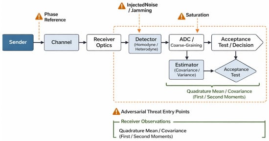
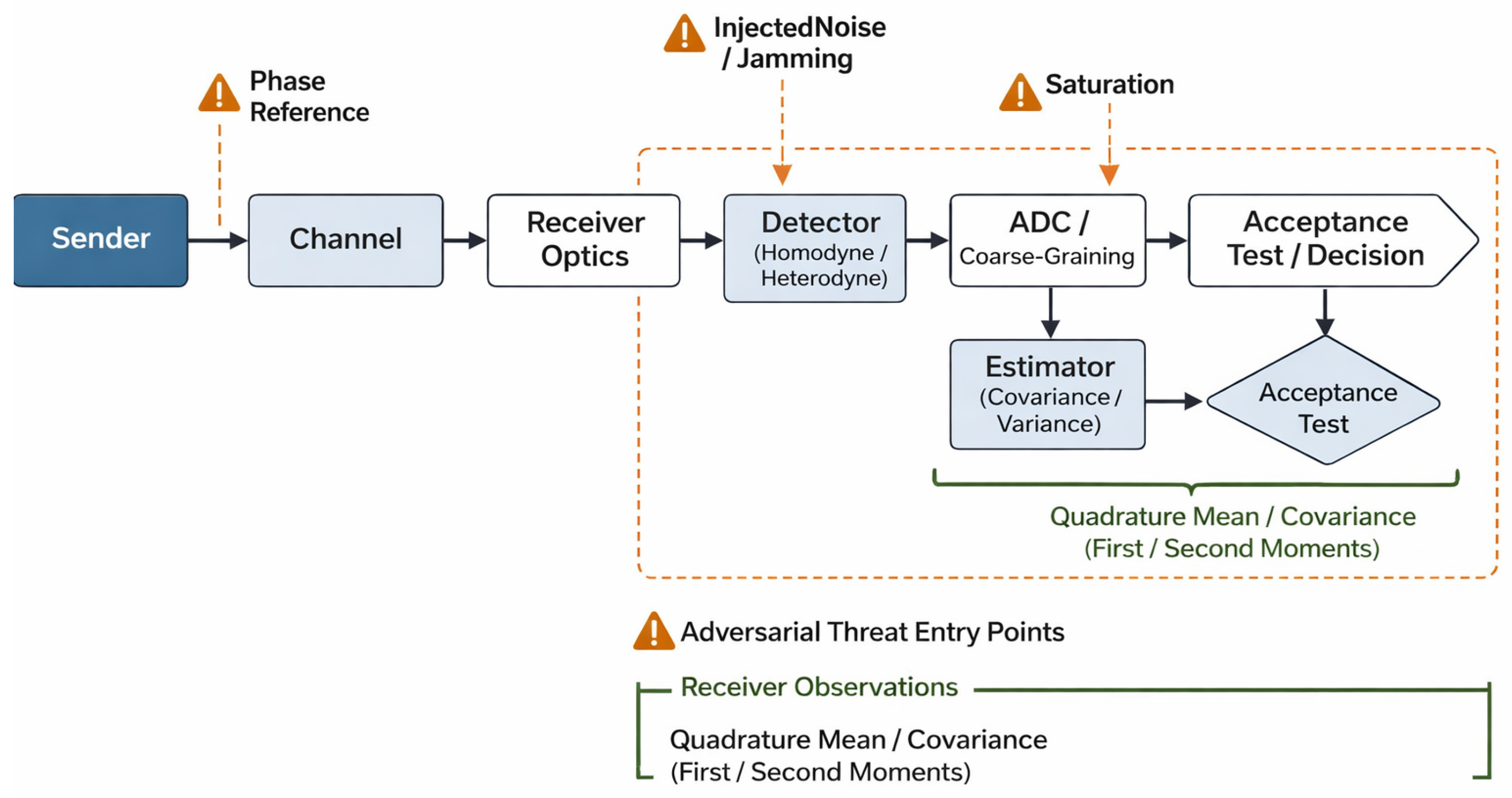
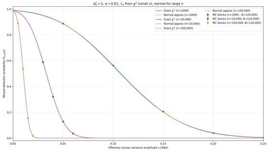
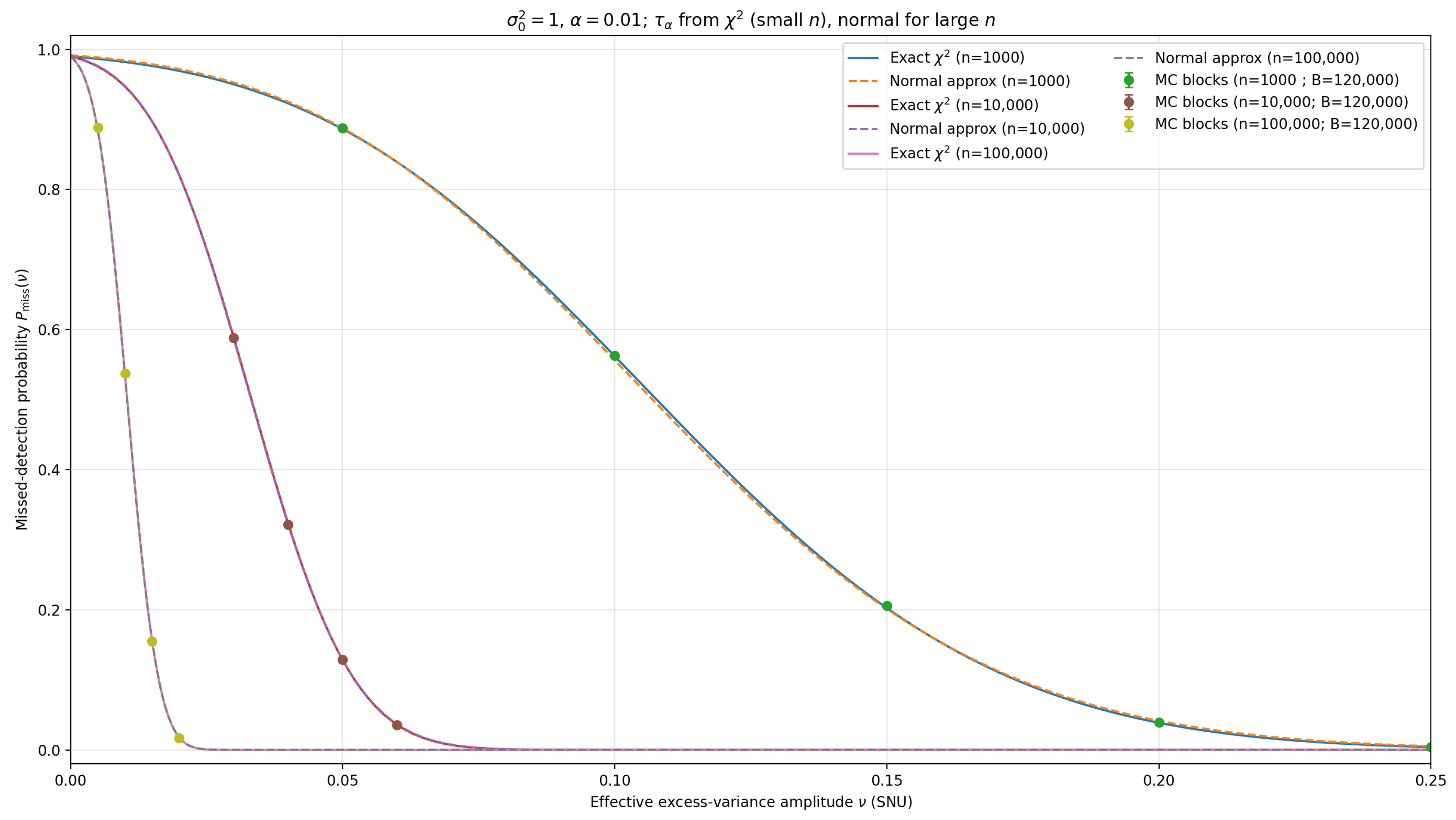

Disclaimer/Publisher’s Note: The statements, opinions and data contained in all publications are solely those of the individual author(s) and contributor(s) and not of MDPI and/or the editor(s). MDPI and/or the editor(s) disclaim responsibility for any injury to people or property resulting from any ideas, methods, instructions or products referred to in the content. |
© 2026 by the authors. Licensee MDPI, Basel, Switzerland. This article is an open access article distributed under the terms and conditions of the Creative Commons Attribution (CC BY) license.