


Abstract
Precise modeling of narrow gorges is challenging due to extreme confinement, hindering visibility and accessibility. These environments often render Global Navigation Satellite Systems (GNSS)-based positioning unfeasible, a difficulty compounded by water and dense vegetation. Consequently, multi-technique data fusion is required. This study proposes a robust methodology to generate high-resolution 3D models of such complex environments by integrating multiple aerial (e.g., Unmanned Aerial Vehicles, UAVs) and terrestrial techniques. A multi-sensor approach combined UAV-Light Detection and Ranging (LiDAR) and UAV-photogrammetry for external areas with Terrestrial laser scanning (TLS), Mobile Mapping System (MMS), and Spherical Photogrammetry (SP) for the canyon floor. Furthermore, the representativeness of these 3D models was analyzed against standard Digital Terrain Models (DTMs) for determining water height levels during flood events. A one-dimensional hydraulic (1DH) model compared the 3D mesh approach with the traditional 2.5D perspective in a challenging, narrow canyon prone to flooding. Our results show that traditional 2.5D DTMs significantly over- or underestimate water levels in narrow sections—failing to account for overhangs and vertical wall irregularities—whereas high-resolution 3D meshes provide a more realistic representation of hydraulic behavior. This work demonstrates that multi-sensor data fusion is essential for accurate flood risk management and infrastructure planning in complex fluvial environments.
1. Introduction
Natural hazards are common in narrow gorges and canyons, frequently conditioned by factors such as topography, geology, and other geomorphological characteristics. Steep slopes and vertical walls create highly favorable conditions for triggering mass movements, specifically landslides and rockfalls [1], and for inducing flash floods [2]. The presence of a drainage network (e.g., rivers, watercourses) at the bottom of these features, whether intermittent or perennial, can lead to a significant increase in flow and water level following episodes of high precipitation. This often results in flash floods either within the canyon or downstream. These complex geomorphic environments are thus recognized globally as high-risk areas, where the co-occurrence of rockfalls and intense flows, or a cascading hazard effect, poses a serious threat to infrastructure and life [3,4]. These intense flows not only increase stream velocity, thereby affecting both the natural environment and infrastructure, but also alter the riverbed through the accumulation or erosion of sediment. This sediment transport is significantly amplified when the stream incorporates other elements, leading to more destructive debris flows [5,6].
In the context of flood modeling, simulation models constitute an important tool for analyzing flood risk and for providing fundamental data to manage the consequences of potential inundations (e.g., spatial extent, water level). They are categorized into hydrologic and hydrodynamic models [7,8]. Hydrologic models address rainfall runoff processes, requiring less computational resources, while hydrodynamic models focus on the physical movement of water. Regarding their spatial domain, these models can be classified into one-dimensional horizontal (1DH), two-dimensional horizontal (2DH), coupled 1DH/2DH, and three-dimensional (3D) approaches. However, 3D hydrodynamic models are highly complex and are not widely used [8], typically being applied only to local scales. Therefore, recent flood modeling studies are mainly based on 2D representations of the terrain topography, such as Digital Terrain Models (DTMs). DTMs can be represented using raster grids and Triangulated Irregular Networks (TINs), which provide a 2.5D representation of the terrain (2.5D models) where each XY position is assigned exclusively one height value. In contrast, 3D meshes represent the terrain surface as a true 3D product, implying that any XY position can accommodate multiple height values. While DTMs facilitate processing and management, 3D meshes provide a more realistic representation of the terrain, especially in areas where the topographic surface is inverted. In 2.5D models, these topographic cases (e.g., overhangs) cannot be represented. This is an important aspect in areas like canyons and gorges, where the terrain can show great irregularity due to erosion processes that generate overhangs and the presence of debris dragged by the stream. However, due to the processing and modeling complexity, most studies conducted to date have used DTMs [7,8] instead of 3D meshes. The use of 2DH modeling is recommended in areas without complex relief and non-inverted areas, providing good results even in large scenes. This aspect is evident in commonly used software applications available in the market (e.g., HEC-RAS v 6.6, TUFLOW v 2025), developed by several institutions and organizations. For example, ArcGIS Pro v. 3.4 includes a flood simulation tool based on 2.5D terrain surfaces [9] and HEC-RAS v 6.6 generates a 2D computational mesh from a DTM [10]. Several studies analyze these software packages, describing their advantages and disadvantages [11,12]. Three-dimensional modelling based on computational fluid dynamics (CFD) is also included in several software packages, such as Flow-3D Hydro v 2025R1 [13].
In the case of gorges and canyons, the presence of inverted surfaces, such as those caused by overhangs, suggests the use of 3D meshes instead of 2.5D terrain models. On the other hand, the demanding computational requirements hinder their wide use in large- and medium-sized environments (e.g., several hectares), especially when considering high-resolution meshes to represent the topography. Therefore, a simplified approach with lower computational requirements but adapted to these complex scenes (e.g., considering the presence of inverted topography) is desirable to simulate flooding events and determine the water level. In contrast to models focusing on XY extension in open scenes, this model should focus on the vertical dimension (or height) due to the specific geomorphological features of canyon and gorge environments.
The evolution of geomatic techniques (e.g., photogrammetry, LiDAR) during the last decades has enabled the acquisition of high-resolution terrain models, even in complex scenes. The integration of sensors (e.g., digital cameras, LiDAR) on Unmanned Aerial Vehicles (UAVs) [14,15,16] allows data acquisition from elevated viewpoints (from a few meters to tens of meters), thus obtaining better coverage of the object and avoiding occlusions. Multiple studies focus on improving data acquisition and processing efficiency by applying new techniques and devices. In photogrammetry, the use of lenses with a higher field of view (FoV) (e.g., wide-angle and fisheye lenses) [17] improves data acquisition and processing by reducing the number of photographs needed to cover a scene. This is crucial in complex cases where the number of images can drastically increase when using normal lenses. An additional improvement is achieved with Spherical Photogrammetry (SP) [18] by using panoramic images, such as those generated with 360-degree multicameras (composed of several fisheye lenses). Furthermore, the implementation of Mobile Mapping Systems (MMS) [19,20] has shown significant improvement in data acquisition efficiency. These systems are based on the calculation of the trajectory and orientation using Simultaneous Localization and Mapping (SLAM) (visual-SLAM or LiDAR-SLAM) supported by Global Navigation Satellite Systems (GNSS) (outdoor surveys) and Inertial Navigation System (INS). These advancements have also been simultaneously supported by software and hardware improvements. The development of algorithms that facilitate image processing (e.g., Structure from Motion—SfM [21,22] and dense Multi-View Stereo—MVS [23,24]) and point clouds alignment (e.g., Iterative Closest Point—ICP [25]) and their implementation in various software packages (e.g., Agisoft Metashape v 2.2.2 [26], Cloud Compare v 2.14 [27]) have enabled multiple applications of geomatic techniques in geosciences. In most cases, the use of a single technique has proven sufficient to obtain a comprehensive model of the reality to be used in flooding studies [28]. However, other cases require multiple techniques, leading to approaches based on data fusion [29,30]. This is the case of complex scenes characterized by narrow spaces, non-accessible areas, multiple occlusions, and difficulties in using specific techniques (e.g., Global Navigation Satellite Systems—GNSS). In such narrow gorges and canyons, accessibility to specific areas is often difficult or impossible, requiring the integration of multiple techniques, both aerial and terrestrial, to obtain a comprehensible model of the scene.
In this context, this study represents an adaptation and improvement of previous work developed by our team [31]. This previous approach consisted of a new methodology based on data fusion to model complex scenes related to narrow gorges, which was applied to the Caminito del Rey (Málaga, Spain). Thus, multiple aerial and terrestrial techniques (photogrammetry and LiDAR), including static (e.g., Terrestrial Laser Scanning—TLS) and mobile systems (MMS), were implemented jointly to take advantage of each technique’s strengths. Building upon this previous experience, this study focuses on generating high-resolution 3D models to analyze water levels during flooding events, in contrast to previous work focused on assessing rockfalls affecting boardwalks. This presents a higher challenge because it is focused on the bottom areas of the gorges and canyons, where stream flows, and where difficulties arise due to narrow spaces, occlusions, and null satellite coverage (e.g., making GNSS unusable for georeferencing). In this sense, this study includes methodological improvements (e.g., determining the coordinate reference system in narrow spaces) and the generation of new products designed specifically for this new purpose.
Objectives
The primary aim of this research is to develop a robust methodology for generating high-resolution 3D models of complex gorge environments, ensuring comprehensive scene coverage and paying special attention to the bottom areas of gorges and canyons where stream flows. To achieve this primary goal, the study focuses on the following specific objectives:
- To establish and implement an advanced multi-sensor data fusion procedure combining data from various geomatic techniques, including both terrestrial and aerial imagery (photogrammetry) and LiDAR technology, while ensuring high geometric accuracy.
- To analyze the results obtained from these techniques, considering data completion.
- To propose an alternative, practical georeferencing strategy that overcomes the typical limitation of inaccessible positioning, such as the total lack of GNSS coverage in narrow canyon settings, to locate all generated products accurately.
The secondary goal is to compare the high-resolution 3D model against several commonly used 2.5D terrain models by evaluating water level accuracy during flood events. Specifically, this study analyzes how inverted topographic surfaces (e.g., overhangs), which are accurately captured in 3D meshes, influence hydraulic results compared with 2.5D representations.
The effectiveness of this proposed methodology will be validated by its application to a narrow and geometrically complex case study, where a detailed 3D model is required for tourist route planning (including a boardwalk) and the mitigation of identified geohazards (e.g., flooding).
2. Methods and Materials
The methodology developed in this study is divided into two main sections. The first focuses on obtaining high-resolution 3D documentation of narrow gorges and canyons. The second focuses on the analysis derived from the previously generated 3D model to analyze water height considering different flows.
2.1. 3D Documentation
The 3D documentation of narrow gorges and canyons relies on multiple geomatic techniques due to the environmental challenges of these scenes. Our approach integrates aerial (LiDAR-UAV and image-UAV) and terrestrial (TLS, MMS, and SP) techniques. Aerial methods focus on the upper areas, while terrestrial methods are applied to the canyon floor and lower walls, where accessibility is constrained and occlusions are prevalent.
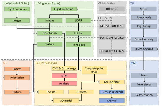
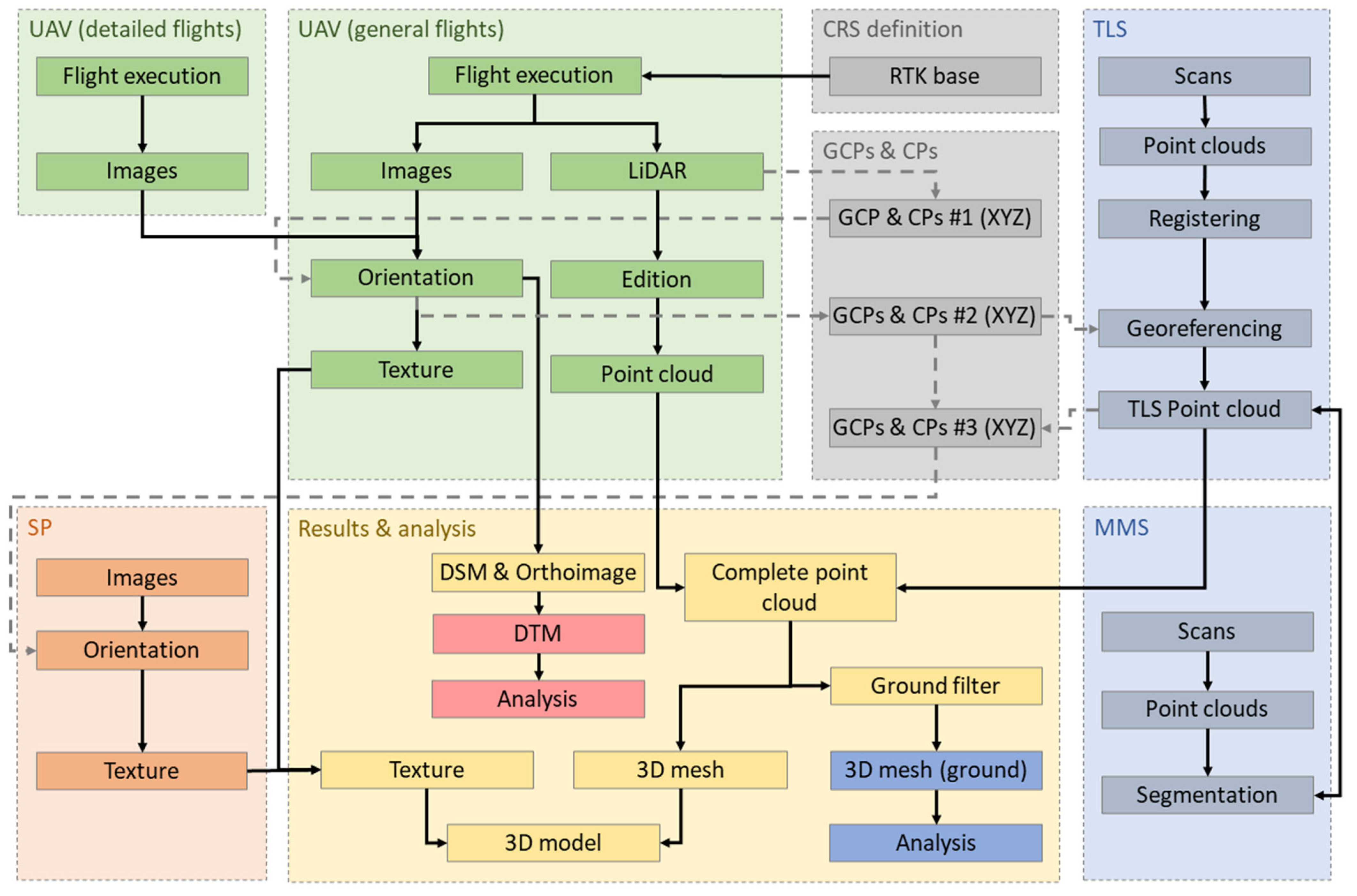
Data fusion is essential to achieve complete coverage; however, this process must account for the varying accuracy and precision of each sensor. Consequently, this approach prioritizes data from the most accurate sources (e.g., TLS point clouds), while secondary data (e.g., UAV LiDAR) are initially used to fill gaps in uncovered areas. The proposed 3D documentation workflow is summarized in Figure 1, representing an improvement and adaptation of previous works [31] to the specific purposes of this study.
Figure 1.
Methodology for 3D documentation proposed in this study.
2.1.1. Coordinate Reference System Definition
Defining a Coordinate Reference System (CRS) is one of the main challenges in these environments. Traditional surveying and GNSS are often unfeasible due to narrow spaces and occlusions that block both visual observations (total station) and satellite signals. Therefore, aerial techniques—positioned via GNSS-RTK (Real Time Kinematic)—are used to establish the primary CRS. Once aerial products are georeferenced, terrestrial data are aligned using a hierarchical strategy of Ground Control Points (GCPs) or the ICP algorithm. This procedure is evaluated using Checkpoints (CPs).
As shown in Figure 1, the georeferencing hierarchy is established as follows:
- GCPs & CPs #1: Extracted from the UAV LiDAR point cloud (pre-georeferenced via GNSS-RTK) to orient the aerial photogrammetric block.
- GCPs & CPs #2: Derived from the oriented photogrammetric block (general and detailed flights) to georeference the Terrestrial Laser Scanner (TLS) data.
- GCPs & CPs #3: Extracted from the georeferenced TLS point cloud to provide spatial control for the orientation of spherical photogrammetry (SP).
2.1.2. UAV Flights
The methodology proposed in this study includes two types of UAV flights: a general flight that provides data from a top view of the scene, and detailed flights developed to obtain data of vertical walls and bottom areas. The general flight includes both LiDAR data and images, providing point clouds and a photogrammetric block. LiDAR data are edited to obtain a final point cloud of the scene. The system is pre-georeferenced using a GNSS-RTK correction. Conversely, the photogrammetric block is composed of images obtained from the general and the detailed flights. These images are oriented using a set of well-defined GCPs obtained from LiDAR data, with this process being checked using a set of CPs. Orientation is based on SfM and MVS algorithms [21,22,23,24]. The photogrammetric process yields a texture of most of the scene, a Digital Surface Model (DSM), and a nadir orthoimage.
2.1.3. Terrestrial Laser Scanning and Mobile Mapping Systems
Despite the inclusion of LiDAR data from aerial platforms, the presence of narrow spaces and occlusions probably causes gaps in the definition of the geometry of the scene. In this regard, the methodology incorporates terrestrial capture techniques based on LiDAR to complete the previously obtained point cloud. Therefore, this point cloud is determined using both static (e.g., TLS) and mobile techniques (e.g., MMS). The first (static) is the main data source to define the geometry of the scene (TLS point cloud). It is based on a laser scanner (TLS) that captures a point cloud from each scanning station. These point clouds are subsequently registered using the ICP algorithm [25]. Therefore, they must contain large overlaps between adjacent scanning stations. After that process, the point cloud is georeferenced using a set of well-defined GCPs extracted from UAV flights. The second technique (MMS) is developed to complete the TLS point cloud in cases where the scene is not fully completed due to the presence of obstacles and occlusions. The inclusion of multiple TLS scanning stations can significantly increase capture time without guaranteeing complete coverage of the scene. In this sense, the use of mobile handheld systems provides continuous capture from multiple viewpoints, improving efficiency despite lower accuracy. The MMS can also be attached to a mast, providing more maneuverability and allowing capture from other viewpoints in order to avoid occlusions. However, the use of MMS introduces certain problems that significantly impact accuracy. One of the main problems is related to drift effects [20], which significantly impact accuracy and increase with the length of the capture. Capture using short and closed rings can help to reduce this issue, but does not remove it. In this sense, our approach includes a segmentation of the MMS point clouds, which are then registered segment by segment to the TLS point cloud using the ICP algorithm. This requires the presence of large overlaps between both datasets. Once the TLS point cloud is completed, it defines the basis of the final point cloud that is completed with LiDAR data from UAV.
2.1.4. Spherical Photogrammetry
SP is developed to complete the texture obtained from the UAV flight images. This is mainly focused on the bottom areas of the canyon, where data are not captured from aerial platforms. In this sense, the use of SP provides high efficiency by using both static (fisheye images) and mobile captures (video). Our approach includes the use of a 360-degree multicamera to obtain complete coverage of the scene with large overlaps. In addition, knowledge of the extrinsic parameters of the camera, defined after a full calibration, facilitates the orientation procedure because the distance between sensors is defined as a constraint of the system [32]. Moreover, the orientation is based on a set of GCPs mainly obtained from the TLS point cloud. As a result, this technique provides a texture that complements that obtained from UAV flights.
2.1.5. Products
Multiple products are obtained as results. The final point cloud and texture are used to obtain a high-resolution 3D model of the scene. A DSM and a derived DTM can be determined to perform 2DH modelling. The final point cloud is used to obtain a 3D mesh of the ground (by including a ground filter), which is also used to analyze water height.
2.2. Experimental Design and Performance Evaluation
To evaluate the advantages of using high-resolution 3D models in hydraulic modeling within these environments, this study presents an experiment comparing water height and velocity results derived from a hypothetical flow event using both a 3D mesh and a traditional 2.5D terrain model. Our approach aims to quantify the distortion introduced by 2.5D models—obtained from various methods and sources—and the influence of river geometry definition on hydraulic outcomes. The specific methodology for determining these hydraulic parameters is detailed in the following section. The process involves defining cross-sections and calculating height and velocity at each section through an iterative method. The method was applied to a case of a narrow gorge located in Spain (described in Section 2.4). This was implemented using a custom software tool developed in Python v. 3.11. Finally, a statistical analysis of the results was conducted to quantify the improvement in accuracy when using 3D models instead of 2.5D representations in these complex terrains.
2.3. Analysis of Water Height and Flow Velocity
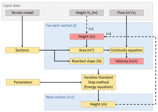
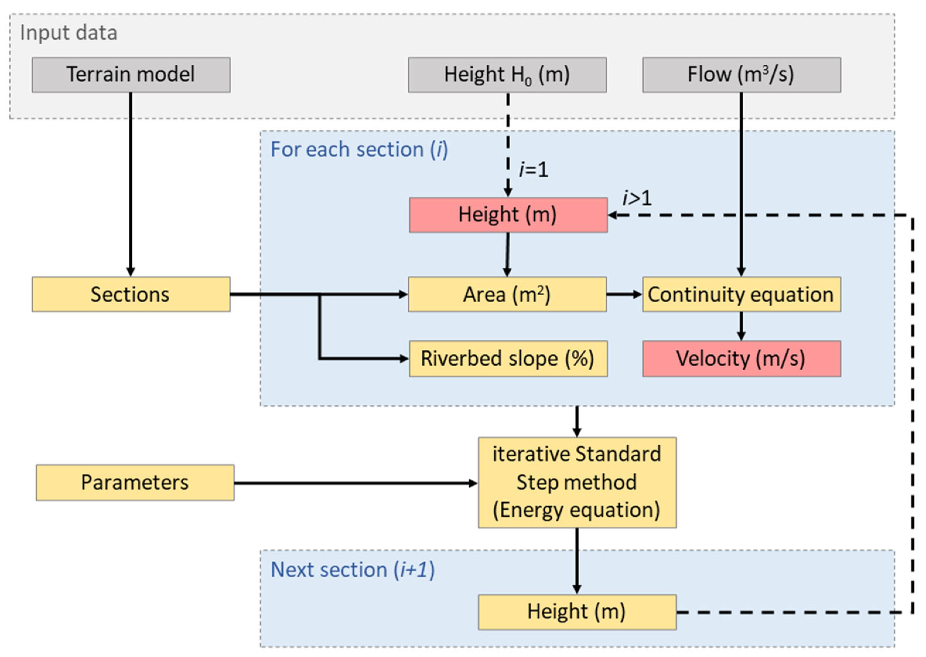
The general workflow for analyzing water levels and flow velocities following flood events is illustrated in Figure 2. The primary objective is to evaluate the influence of different terrain models on hydraulic parameters using a simplified energy-based model. To streamline the calculations, our approach utilizes cross-sections extracted from the terrain models at predefined intervals. The input data include the canyon geometry (3D mesh or 2.5D DTM), the estimated peak discharge (Q), and an initial water height (H0) at a reference section located downstream. To calculate the water level and velocity at each section, the following assumptions and simplifications were made: (i) flow velocity is assumed to be uniform across each individual cross-section (though it varies between sections), and (ii) the influence of vegetation or submerged objects not captured in the terrain models is excluded.
Figure 2.
Procedure to obtain water height and speed values at each section (results at each section are displayed in red color).
Based on these premises, an iterative process was developed to determine the water height and velocity for each section upstream. First, the cross-sectional area (A) is calculated based on the water level. Then, the continuity equation (Equation (1)) [33] is applied to derive the following velocity:
where V is the velocity (m/s), Q is the flow rate (m3/s), and A is the cross-sectional area (m2).
Once the water height and velocity are established for a given section, the values for the adjacent section are determined by solving the energy equation (Equation (2)) using the iterative Standard Step method [34], a procedure also employed by the HEC-RAS software [35]:
where Z is the elevation of the riverbed, Y is the water height (flow depth), α is the velocity weighting coefficient, V is the velocity (m/s), g is the gravitational acceleration (m/s2) and hf represents the total head loss between cross-sections 1 and 2.
This procedure is performed for all sections within a specific terrain model and then repeated for alternative models using identical parameters. This allows for a rigorous comparison to validate the advantages of 3D modeling over traditional 2.5D data in complex environments.
2.4. Case Study
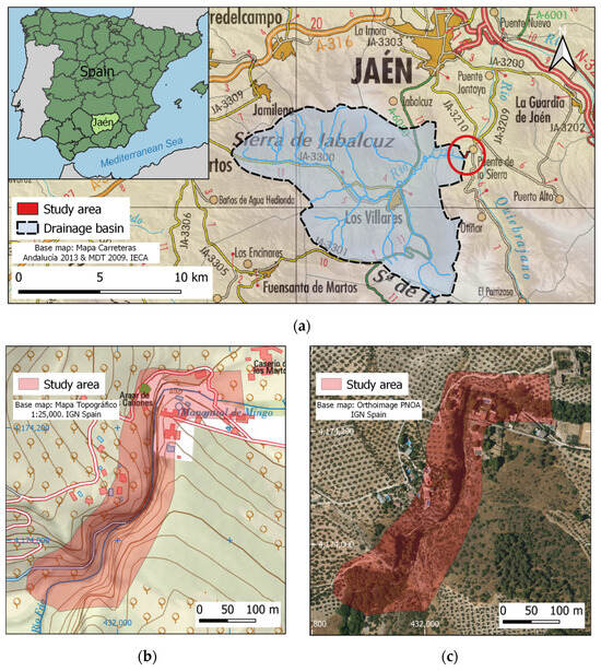
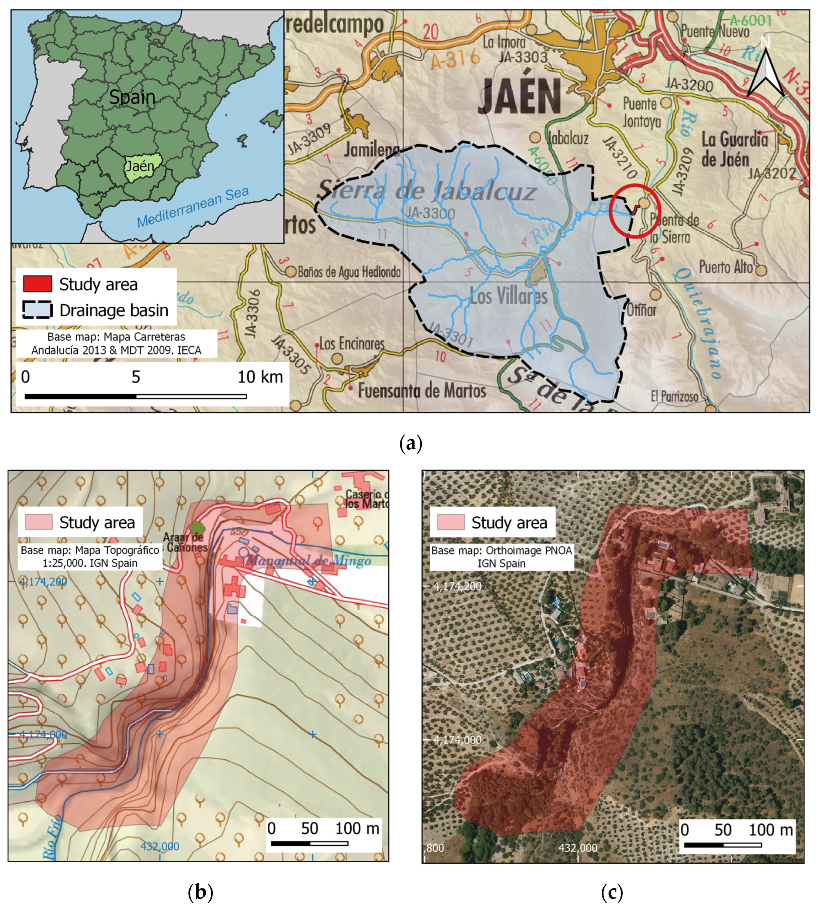
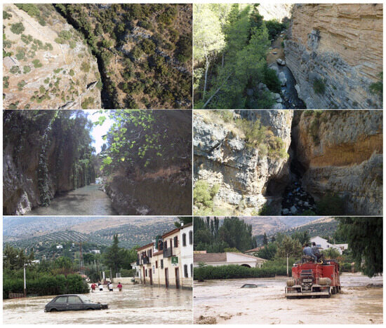
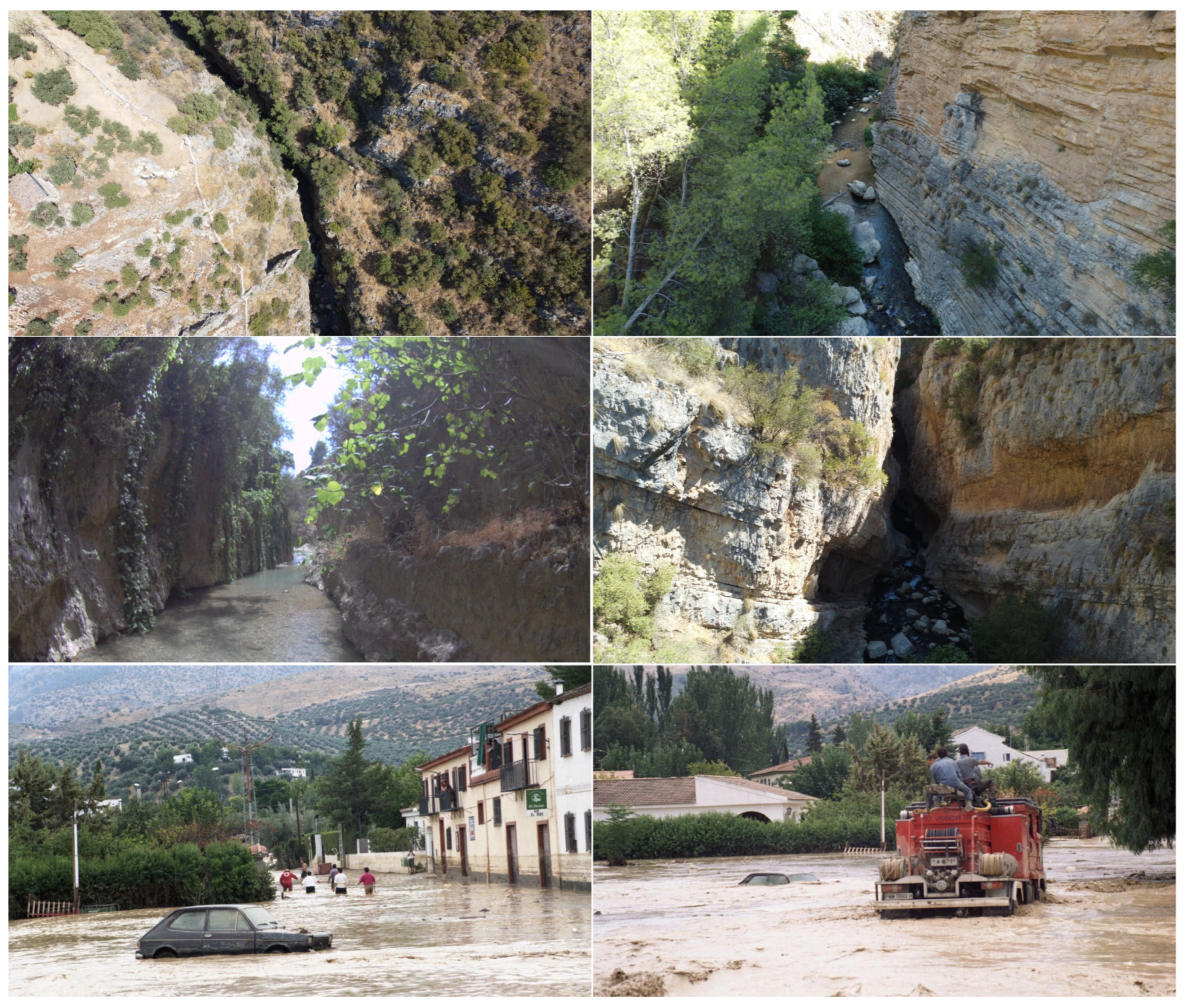
The natural site of Los Cañones de Río Frío (Río Frío canyons) is located next to the city of Jaén in Spain (Figure 3a). The geological context is defined by the river’s intense erosive action on a limestone formation. The geology of the area features relevant structural characteristics, such as a synclinal fold, and specific sediment deposits, including olistostromes. The canyons were formed by the deep incision of the Río Frío, which, over more than 2 km, has carved deeply into the landscape. This process of fluvial erosion has resulted in a landscape with vertical walls that, in some sections, exceed 200 m in height. The drainage basin upstream of the canyon’s location extends over about 10,000 hectares (Figure 3a), which can be considered a small basin characterized by mountainous relief. This study focuses on the northeastern area of these canyons, where the narrowest and most complex gorges are located. Thus, the study area extends along 600 m of the river, covering a total area of about 6 hectares (Figure 3b) and including a narrow canyon with rock walls up to 70 m high and separated by only 1.8 m in some areas, with a mean value of 7 m (Figure 4). The area presents large rock blocks on the riverbed and abundant vegetation (e.g., olives, pines, and ivy) on the banks (Figure 2).
Figure 3.
Location of Río Frío canyons: (a) general location including the drainage network; (b) map of the study area (source: MTN 25,000, IGN Spain); (c) orthoimage of the study area (Source: PNOA, IGN Spain).
Figure 4.
Images of Los Cañones de Río Frío and consequences of the flooding that occurred downstream in 1996 (source: jaenhoy.es).
This area has experienced several flood events, the latest in January of 2026, with multiple effects both inside the canyon, reaching a considerable water level, and causing significant damage in a village located 1 km downstream. For example, Figure 4 shows the consequences of a flood event that occurred in a town located downstream (Puente de la Sierra) in 1996. During this event, precipitation was not exceptionally high across the basin (about 75 mm over several hours), but the stream flow increased due to the geomorphologic features of the canyon [36] and the possible presence of natural dams that were destroyed by the stream, releasing the accumulated water.
In this context, local institutions are developing a plan for the tourist use of this area, including a route with boardwalk trails attached to the rock. The planning includes using a 3D model of the area to analyze the possible location of the walkways while considering flooding hazards. Therefore, the required 3D model must be high-resolution (centimeter-level).
3. Application and Results
3.1. 3D Documentation
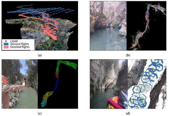
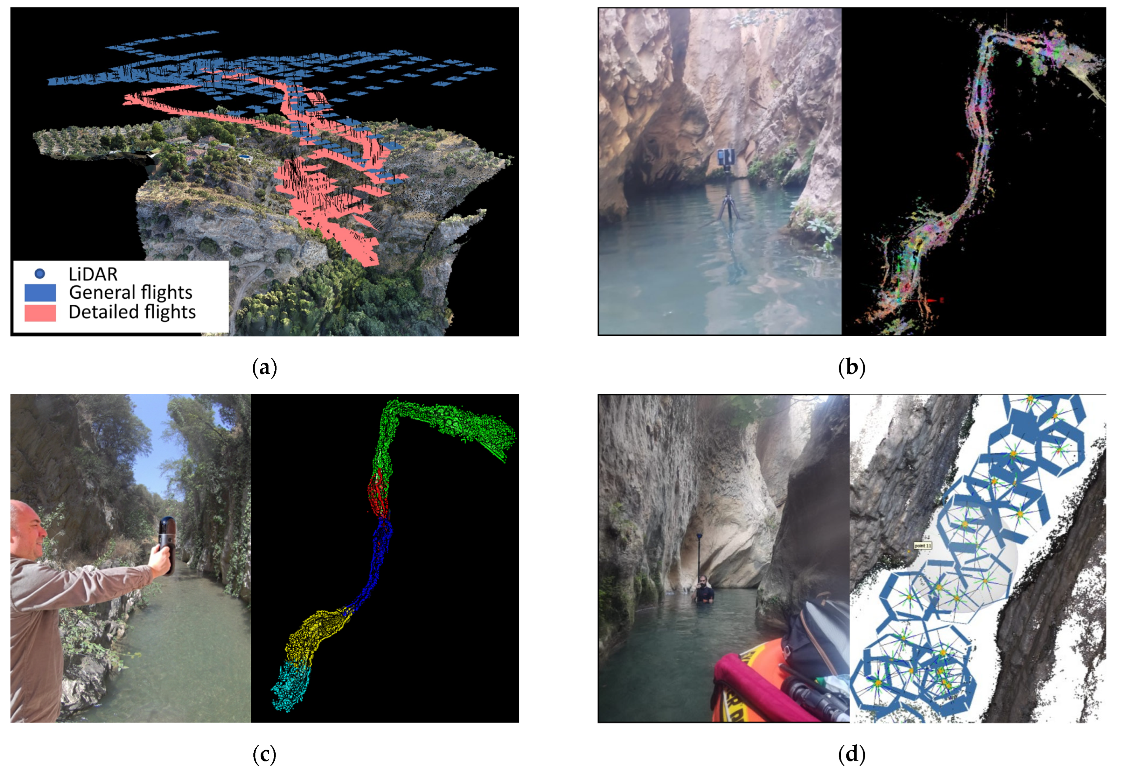
The methodology proposed in this study was applied to the case study described in Section 2.4. Sensors used in this application are described in Appendix A. Due to the difficulties of the area, the CRS definition was based on a GNSS-RTK base that provided differential corrections for UAV positioning. Thus, for general flights, we used a DJI Matrice 300 RTK UAV (Table A1), which includes a LiDAR sensor (DJI Zenmuse L1), an optical sensor, and various devices that enable centimeter-level positioning using RTK corrections. The flights were planned and developed following the suggestions described by Gómez-López et al. [37] for mountainous areas, which included the definition of strips considering terrain elevation and large overlaps. In this sense, during planning tasks, we used a preliminary DTM obtained from the PNOA LiDAR product, published by the Instituto Geográfico Nacional (Spain). Thus, we developed a flight following the river trace and another perpendicular to it. General flights provided a LiDAR point cloud of about 160 million points with a mean point spacing of 3 cm. These LiDAR data were processed using DJI Terra v 4.2.5 software [38] to determine the trajectory and generate the point cloud, and BayesMap StripAlign v 2.24 software [39] to adjust strips and reduce noise within the point cloud (Figure 5a). A set of GCPs and CPs was extracted from the point cloud for the orientation of photogrammetric data by considering well-defined features. Finally, this point was homogenized to an 8 cm point spacing. In addition, general flights also captured 310 images that were processed together with those obtained from detailed flights. In this context, we used a DJI Mavic Mini 2 UAV (Table A1) to acquire images of vertical walls and areas not covered by the general flight. We obtained 468 images in several flights that were processed together with those obtained from the general flight using Agisoft Metashape v 2.2.2 software [26] (Figure 5a). Orientation was performed considering the GNSS-RTK positioning of the general flight images and the GCPs extracted from the LiDAR point cloud.
Figure 5.
Examples of the application carried out in this study: (a) view of the UAV LiDAR point cloud and location of images captured in general and detailed flights; (b) TLS acquisition and point cloud obtained after registering; (c) MMS acquisition and five registered point clouds; (d) SP acquisition and example of photogrammetric block composed of fisheye images after orientation.
Terrestrial LiDAR was implemented in two ways: static captures from various adjacent stations distributed along the river using a Terrestrial Laser Scanner (TLS), which was focused on the geometry of the bottom areas of the canyon, and a mobile mapping system mounted on a mast, to supplement the previously-obtained point cloud in those areas with gaps. The TLS was developed using a FARO Laser Scanner Focus3D X130 (Table A1) mounted on a tripod. Due to the existence of narrow spaces, most of the stations were set up inside the river channel (Figure 5b). Stations were located considering large overlaps between adjacent stations in order to facilitate registration between point clouds (represented in various colors in Figure 5b). Data capture was developed without color acquisition to improve field efficiency. In total, we captured 79 scans, providing an equivalent number of point clouds. These point clouds were registered using the ICP algorithm implemented in Maptek PointStudio v 2025 [40] software, obtaining an RMSE of about 1 cm. This error was satisfactory considering the registration difficulties caused by vegetation. This process resulted in a registered TLS point cloud composed of more than 340 million points with a mean point spacing of 1 cm. These data were georeferenced to the general CRS (defined by the UAV LiDAR) via a 3D transformation using a set of GCPs, obtaining an RMSE of about 7 cm. Finally, the final TLS point cloud was homogenized to a 2 cm point spacing.
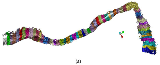
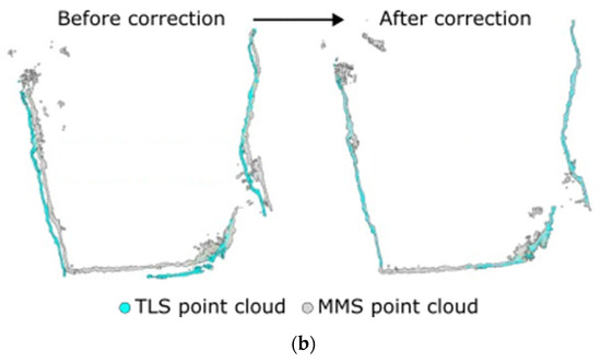
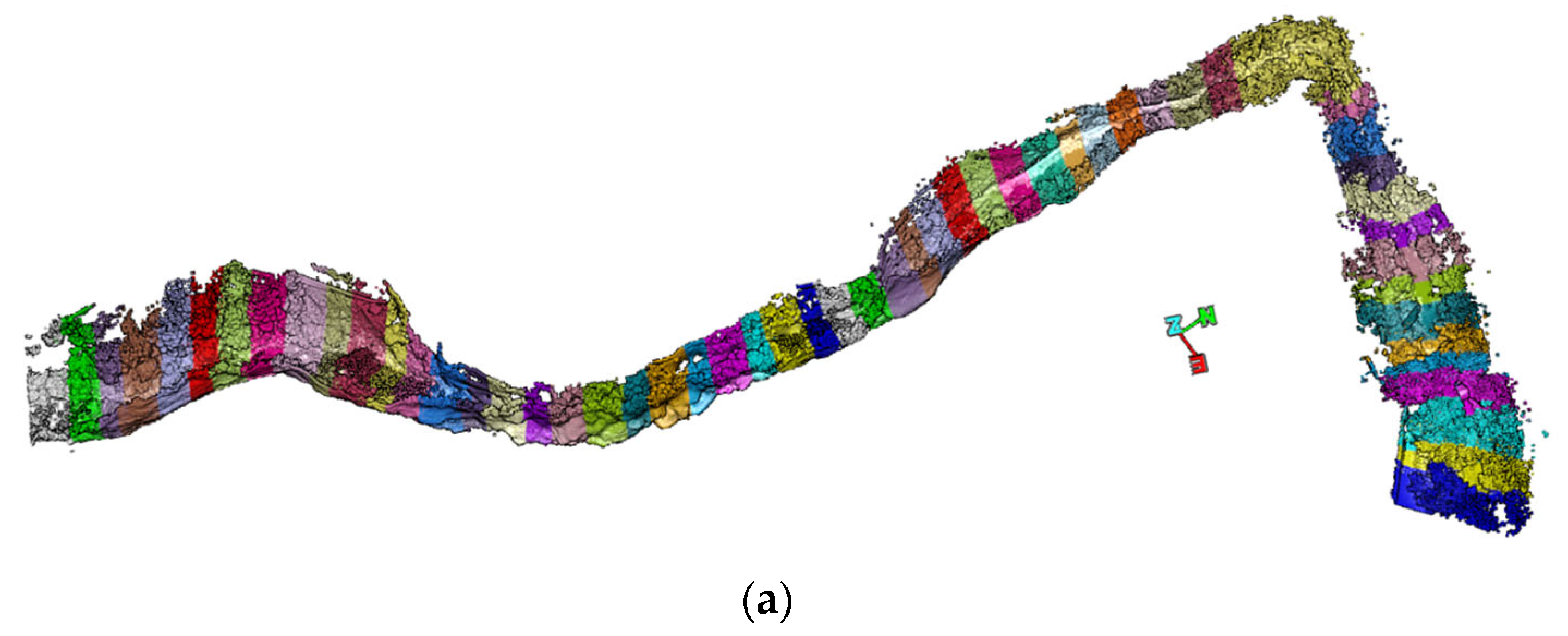
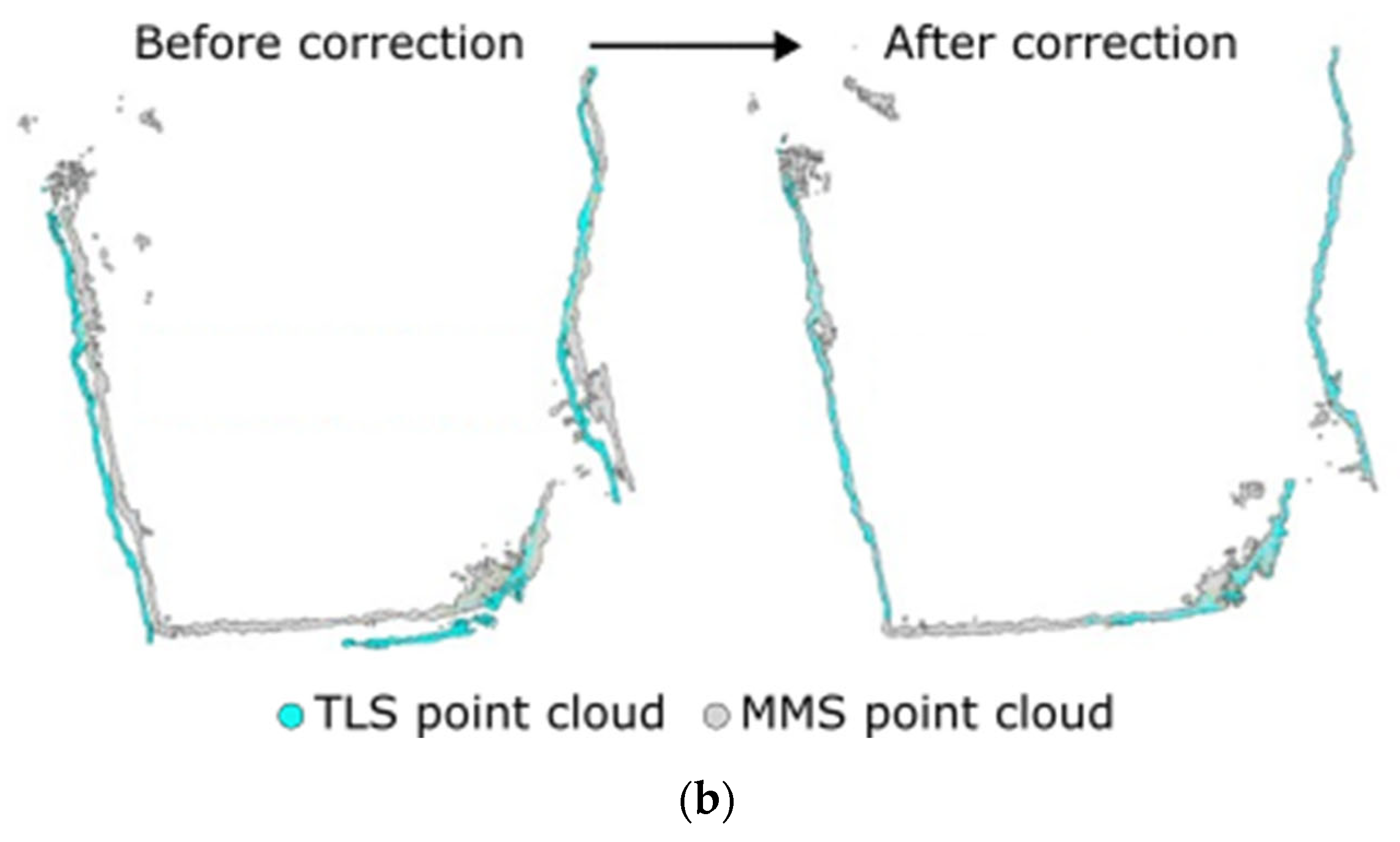
MMS was developed using a handheld Leica BLK2GO (Table A1) (Figure 5c), performing short closed-loop rings to avoid drift effects. We surveyed five scans with significant overlaps to facilitate registration. This process was developed using Maptek PointStudio v 2025 [40] software based on the ICP algorithm, obtaining a final RMSE of about 2.5 cm. The registered point cloud was composed of 89 million points with a mean spacing of about 2.5 cm. This result is noteworthy considering the significant presence of vegetation. The final MMS point cloud was initially georeferenced using the ICP algorithm with the TLS point cloud as the base. However, the results of this process were not completely successful due to discrepancies of about 1 m at the boundaries. These errors were caused by MMS drift issues. Therefore, the registration of MMS point clouds was carried out using the proposed methodology that included a correction based on a segmentation of MMS data (Figure 6). The size of these segments was determined iteratively by reducing their size (Figure 6a) until the MMS data were well-adjusted to the TLS point cloud (Figure 6b). The average size of the segments was about 10 m, with a maximum of 50 m (segments colored in Figure 6a), and the average RMSE was 2.2 cm. The final MMS point cloud was homogenized to a 2 cm point spacing.
Figure 6.
MMS registration process: (a) top view of the segmentation of point clouds; (b) example of TLS and MMS in a cross-section of 50 cm width previously and after the segmentation process. Blue is TLS point cloud; grey is MMS point cloud.
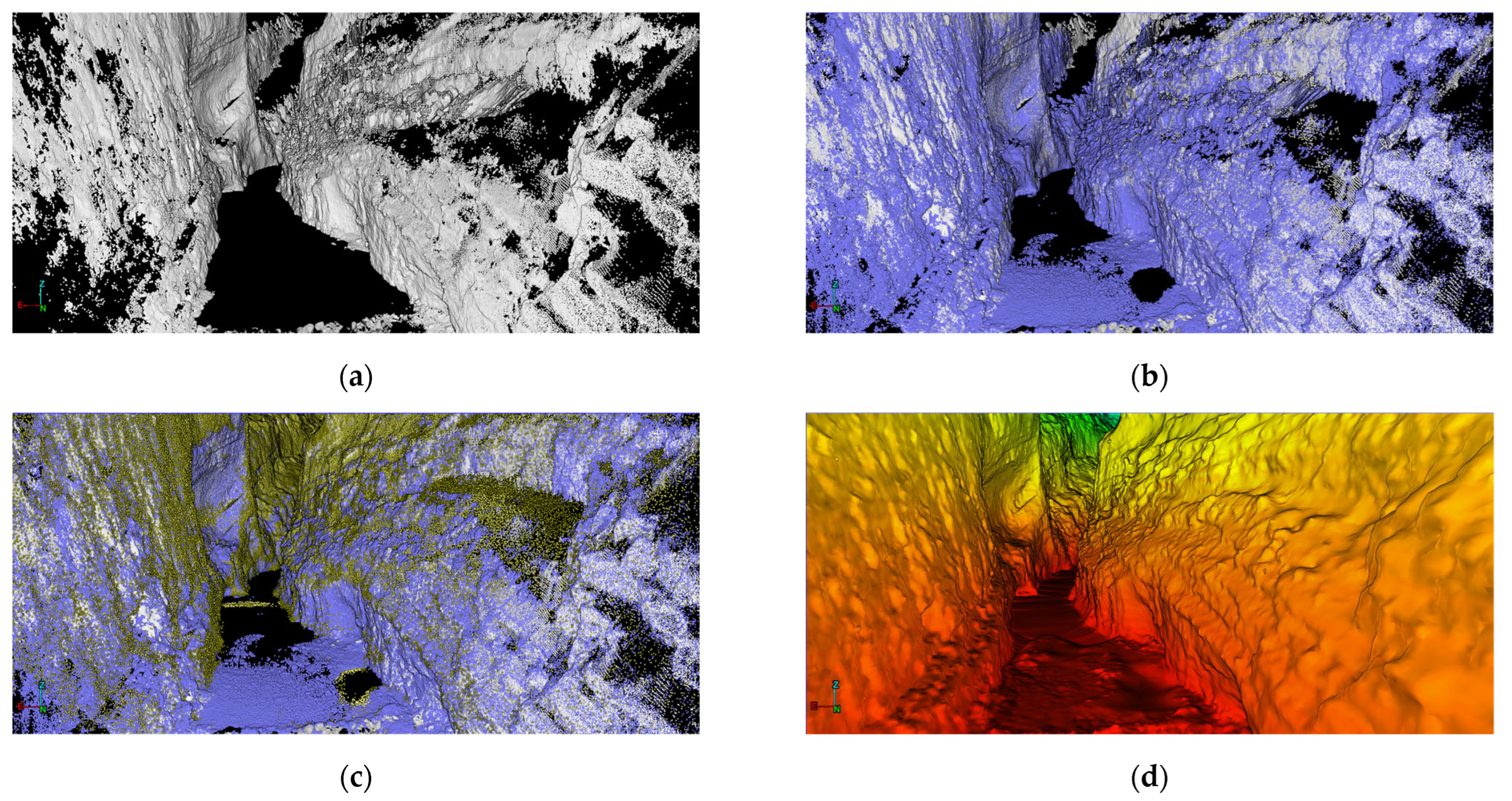
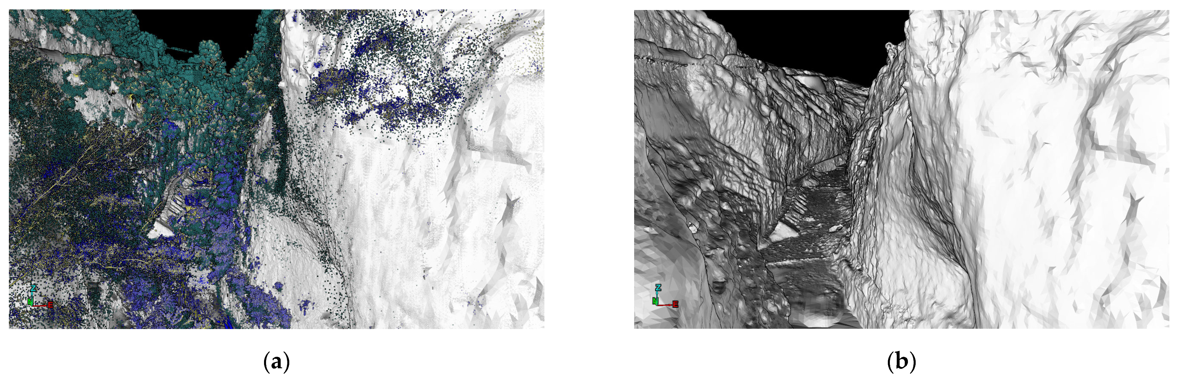
Finally, data fusion between TLS, MMS and aerial LiDAR allowed us to obtain a complete point cloud. Using TLS and MMS, we captured the bottom areas of the canyon, while the higher and external areas were surveyed with the aerial LiDAR. Figure 7 shows an example of the completion obtained by data fusion.
Figure 7.
Example of completion achieved in the final point cloud: (a) TLS (grey); (b) TLS (grey) and MMS (blue); (c) TLS (grey), MMS (blue) and aerial LiDAR (yellow); (d) 3D mesh after data fusion colored by height.
The final point cloud (aerial and terrestrial LiDAR) was classified into terrain and non-terrain points, defining terrain as everything other than vegetation (i.e., terrain, rocks, and canyon walls). This process was performed semi-automatically using the classification and manual editing tools of Lastools v 2025 [41] and Maptek PointStudio v 2025 [40] software. Figure 8 shows an example of this process, where the vegetation, represented by colors in Figure 8a, is removed, yielding the final 3D mesh of the terrain (Figure 8b).
Figure 8.
Example of point cloud filtering: (a) data classified as terrain (grey) and non-terrain (color); (b) 3D mesh of terrain data.
In addition to aerial photogrammetry, we applied SP to obtain the texture of the bottom areas. We used a 360-degree multicamera, a Kandao Obsidian S (Table A1) mounted on a telescopic mast (Figure 5d). This multicamera has 6 sensors and 6 fisheye lenses, providing extensive coverage and overlaps. The camera was fully calibrated, determining the extrinsic parameters that define its geometry. Thus, distances between all sensors were calculated and integrated into the photogrammetric processing by means of scale bars (Figure 5d). This facilitates the orientation of the fisheye images obtained with a separation of about 0.5 m following the riverbed. We covered the entire canyon with 1166 capture stations and 6996 images. The accuracy of the photogrammetric process was about 4.5 cm.
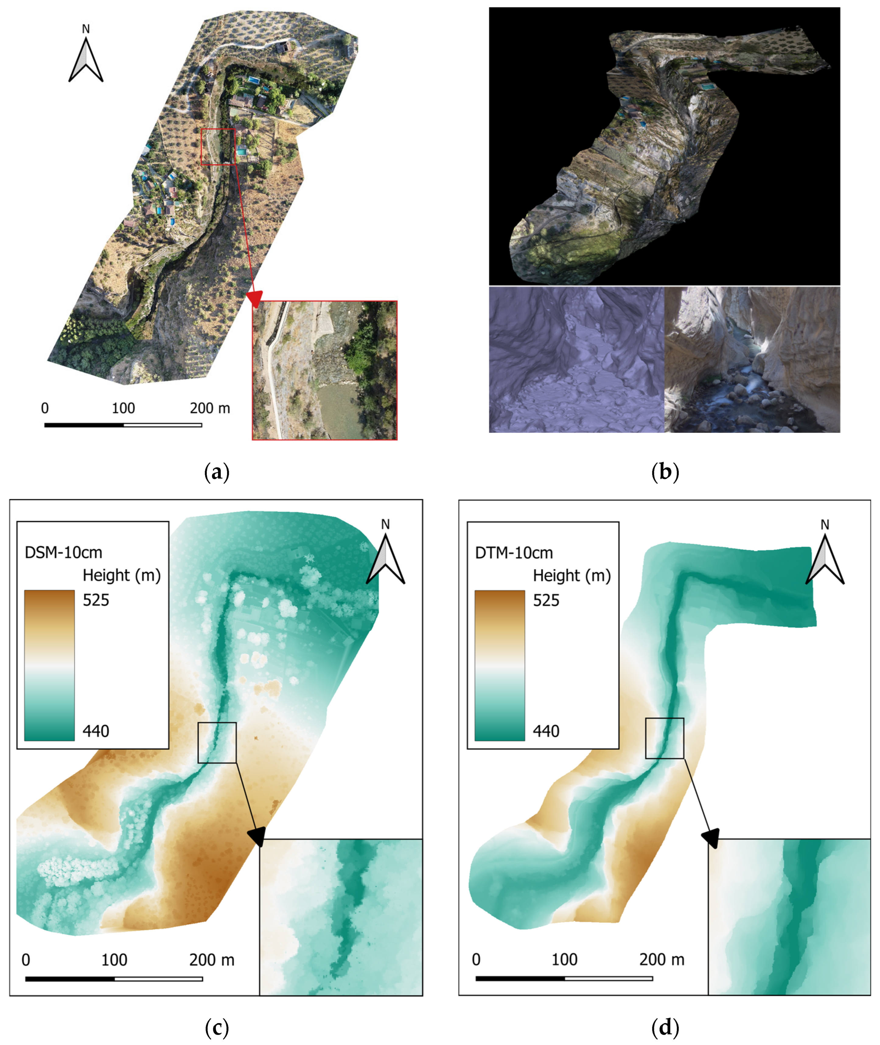
In summary, the graphical documentation of the canyon resulted in multiple products. As a result of the photogrammetric process, we obtained an orthoimage with a 2-cm resolution of the study area (Figure 9a). All photogrammetric blocks were merged into a unique project (aerial and terrestrial), providing a texture that was applied to the 3D mesh to obtain a 3D model of 21 million triangles (Figure 9b). Notably, the use of Spherical Photogrammetry (SP) enabled high-quality texturing in interior areas and underhangs, which would not have been possible using aerial imagery alone (Figure 9b). In addition, we also obtained a DSM with a 10-cm resolution, including vegetation (Figure 9c) and a DTM with a 10-cm resolution without vegetation (Figure 9d).
Figure 9.
Examples of products obtained in this study: (a) Orthoimage of 2 cm; (b) general view of the 3D model and detailed views of 3D mesh and 3D model of a narrow area; (c) DSM of 10 cm; (d) DTM of 10 cm.
3.2. Analysis of Water Height and Flow Velocity
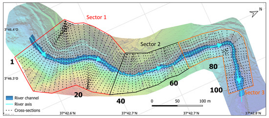
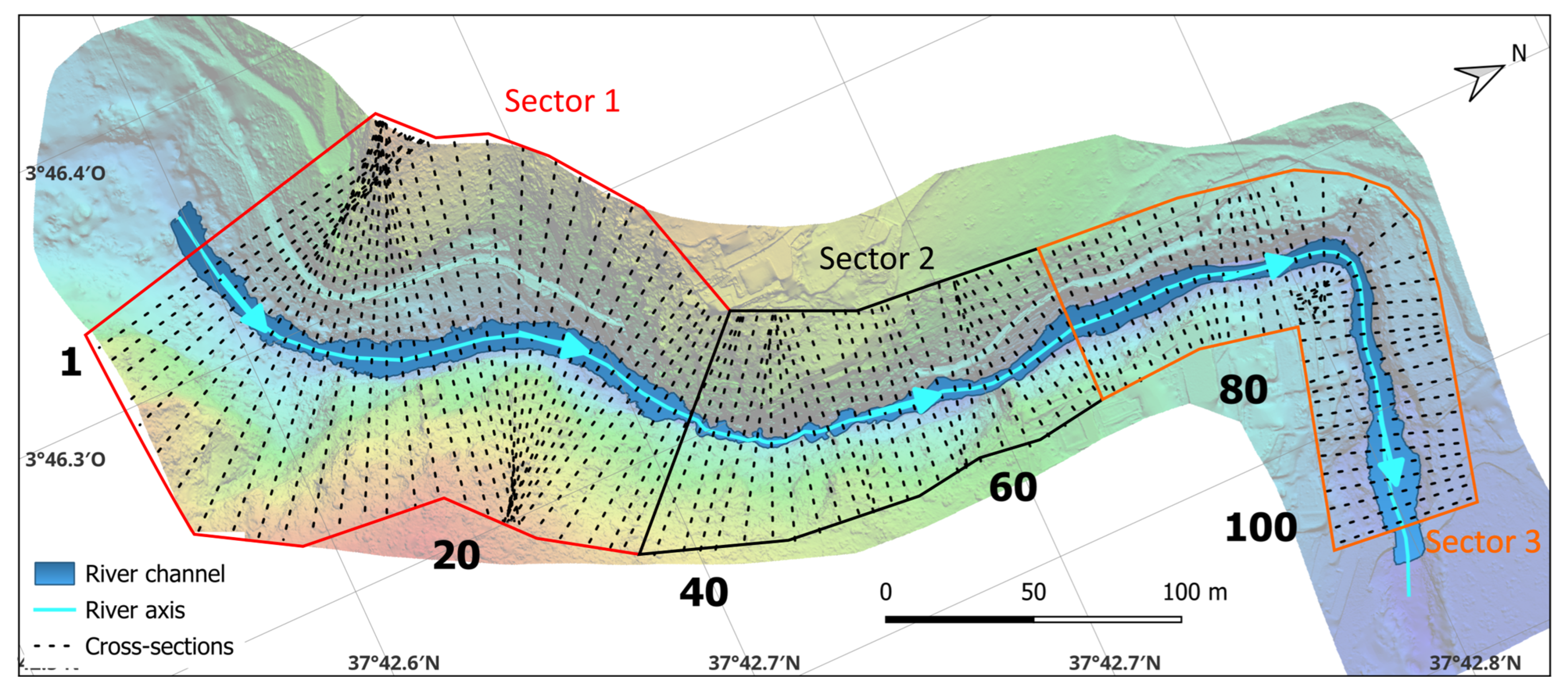
The geometric accuracy of the different terrain models was analyzed by simulating the water height and flow velocity during potential flooding events. The methodology described in Section 2.3 was applied to estimate these parameters based on a predicted discharge (Q) of 232 m3/s (corresponding to a 500-year return period [36]) and an initial water height (H0) of 5.5 m at the downstream-most cross-section. A total of 103 cross-sections were extracted perpendicular to the river axis, spaced at 5 m intervals (Figure 10). To facilitate the analysis, these sections were grouped into three sectors according to the stream direction (Figure 10):
Figure 10.
Location of the cross-sections and sectors defined in this study.
- Sector 1 (S1): Open areas (sections 1 to 36).
- Sector 2 (S2): A narrow canyon reach (sections 37 to 68).
- Sector 3 (S3): A mixed area (open and narrow) including a river bend (sections 69 to 103).
Four different terrain models were evaluated to quantify the impact of dimensionality and resolution on hydraulic outcomes:
- 3DM: The high-resolution 3D mesh generated in this study provides a continuous and true 3D representation of the canyon’s complex geometry.
- DTM1: A 10-cm DTM derived from the 3DM using maximum elevation points (top-view). This represents a scenario where overhangs obscure the channel floor, leading to a predictable reduction in the effective cross-sectional area.
- DTM2: A 10-cm DTM derived from the 3DM using minimum elevation points (bottom-view). This represents the actual riverbed with overhangs removed, resulting in a predictable increase in the flow area compared with 3DM.
- DTM3: A 50-cm DTM derived from IGN (Spain) aerial LiDAR data. Unlike the previous models, this is not derived from a 3D mesh. While aerial LiDAR typically reflects the riverbed (similar to DTM2), the presence of occlusions in narrow, high-confinement areas often distorts the geometry, potentially yielding results more similar to DTM1.
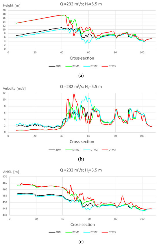
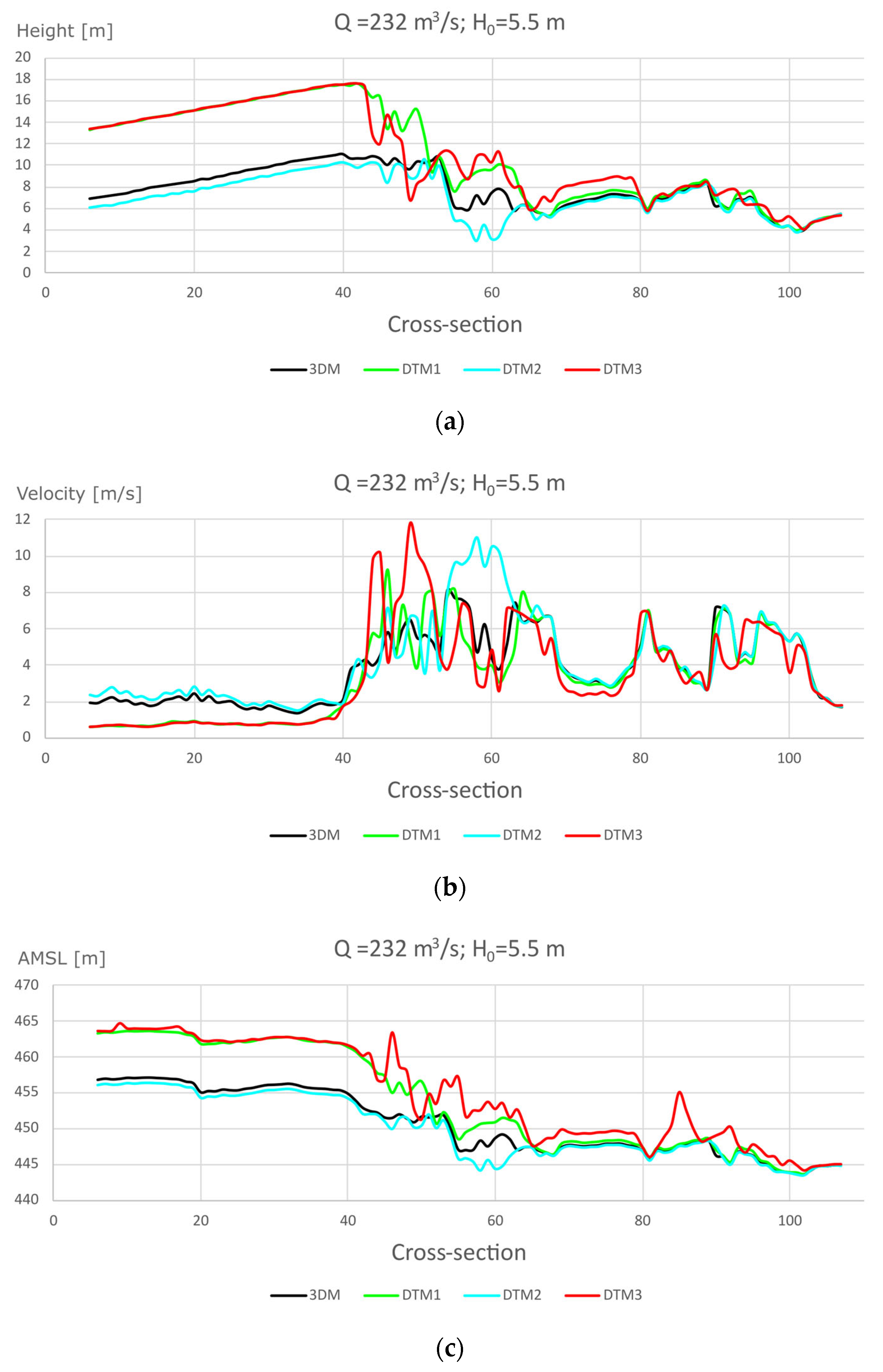
Figure 11 presents the hydraulic results for all 103 cross-sections. Figure 11a illustrates the water height calculated using the energy equation (Section 2.3). The models exhibit similar behavior in open areas (S1 and S3) but diverge significantly in the narrow canyon (S2). In most sections, the 3DM yields intermediate water levels—lower than DTM1 but higher than DTM2. DTM3 shows more irregularities but remains comparable to DTM1 in open areas.
Figure 11.
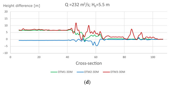
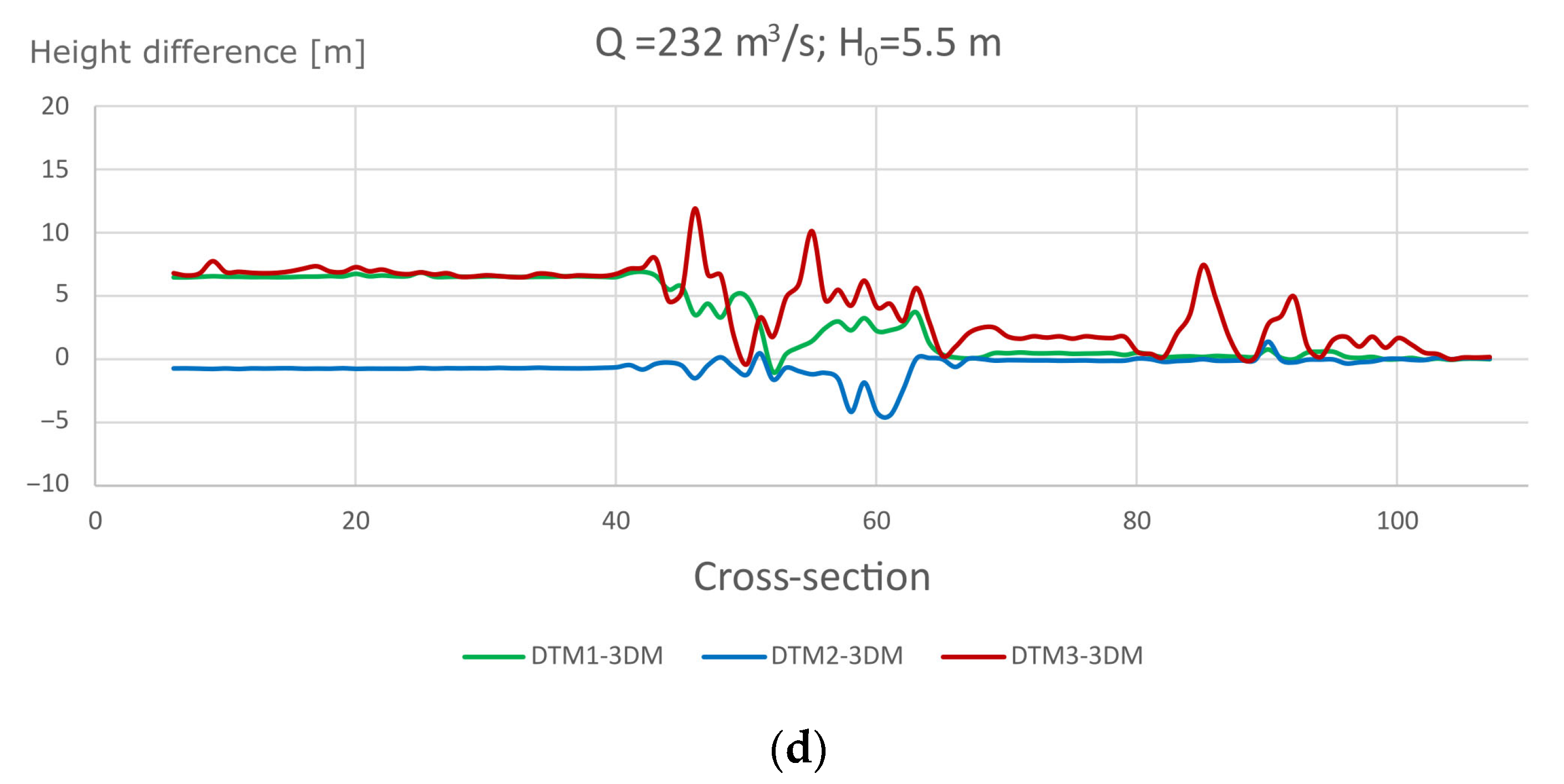
Results by cross-section: (a) water height with respect to the riverbed; (b) flow velocity; (c) water height above mean sea level (AMSL); (d) water height differences of DTM1, DTM2 and DTM3 with respect to 3DM.
Regarding flow velocity (Figure 11b), the profiles generally show an inverse relationship with water height, with higher variability observed in the narrow reach (S2). In S1, flow velocity is lower than in the subsequent sectors, indicating that the narrow canyon acts as a hydraulic bottleneck (natural barrier). This is confirmed by the statistical analysis in Table 1: flow velocity is highest in S2, which also shows the greatest variability (Standard Deviation, Std Dev). Notably, in S1, DTM1 and DTM3 result in lower mean velocities compared with 3DM and DTM2. Furthermore, 3DM velocity values are consistently intermediate between DTM1 and DTM2, with lower overall variability.
Table 1.
Statistics of flow velocity by sectors (S1–S3).
These trends are further supported by the water level analysis (Figure 11c,d). Figure 11c shows the water height above sea mean level (AMSL) by adding the height obtained to the riverbed altitude. The differences between the DTMs and the 3DM (Figure 11d) show that DTM1 and DTM3 mostly over-predict water levels (positive values), while DTM2 under-predicts them (negative values). Statistical results in Table 2 confirm these findings across all sectors, with the highest variability occurring in S2. The Pearson Correlation Coefficient (PCC) indicates a perfect correlation (1.0) in S1 and S3 for DTM1 and DTM2 vs. 3DM, dropping to 0.9 in the narrow S2. DTM3 shows the lowest correlation with 3DM in S2 and S3.
Table 2.
Statistics of water height differences by sectors (S1–S3).
By analyzing both water height and velocity (Figure 11, Table 1 and Table 2), a remarkable difference is observed in S1 between DTM1/DTM3 and DTM2/3DM. This appears to be a direct consequence of the iterative subcritical flow calculation, which progresses upstream. In this regard, the hydraulic discrepancies generated in the narrow area (S2) are transmitted upstream to S1, affecting the entire profile.
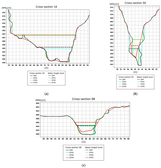
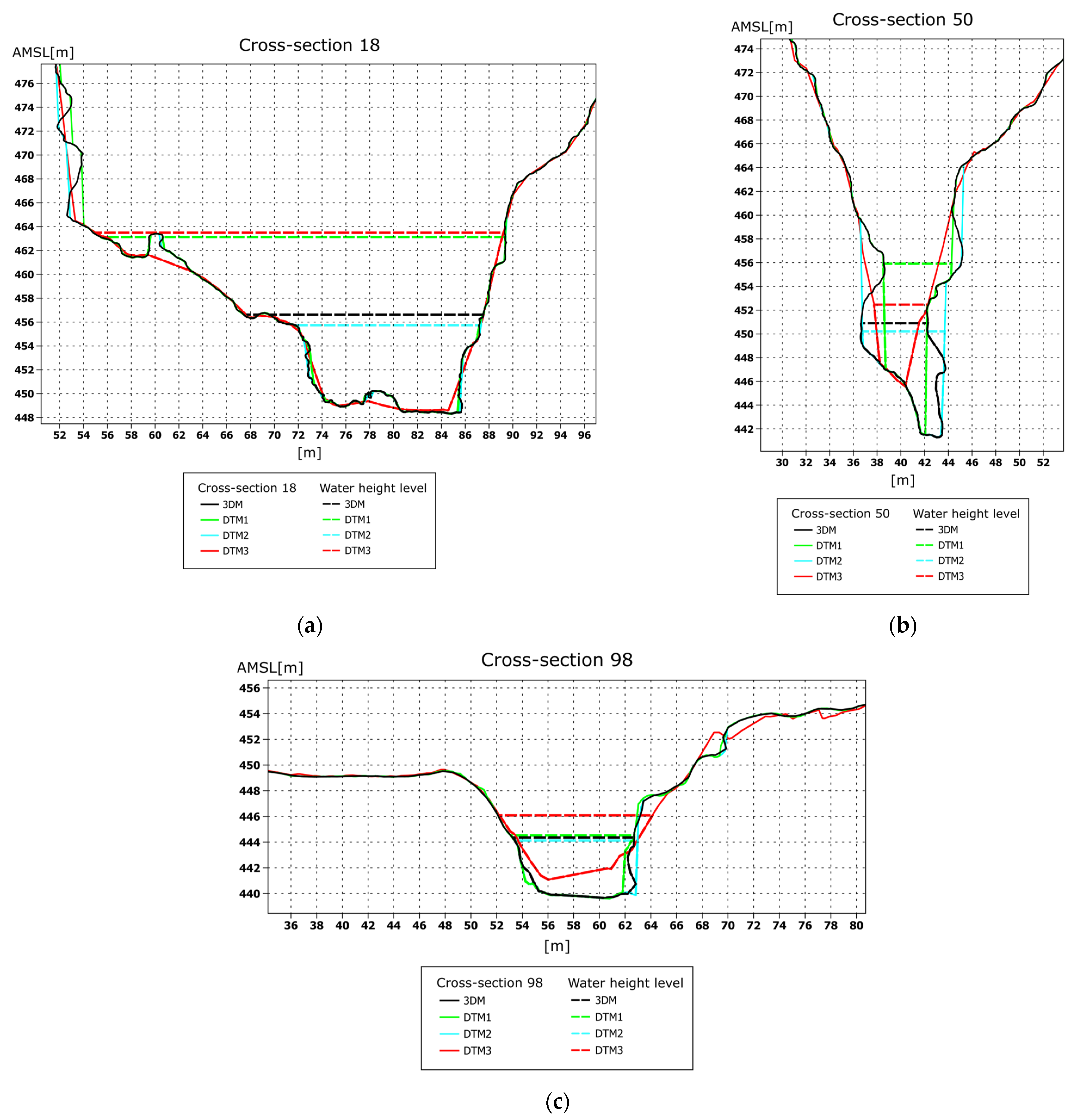
Figure 12 illustrates the geometric differences between the terrain models at representative cross-sections (18, 50, and 98) selected from each sector (S1–S3). This comparison highlights the superior terrain representation of the 3DM, particularly in capturing complex geometries that simplified DTMs fail to accurately represent. Figure 12 also demonstrates that the 3DM water levels are consistently bounded by the other models, with DTM3 and DTM1 yielding the highest levels and DTM2 the lowest. It is worth noting that in cross-sections 50 and 98, the riverbed in DTM3 is not well-defined, leading to an increase in the absolute water level; however, the relative water height remains similar to that observed in DTM1.
Figure 12.
Views of water height level reached in three cross-sections: (a) cross-section 18; (b) cross-section 50; (c) cross-section 98.
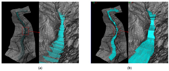
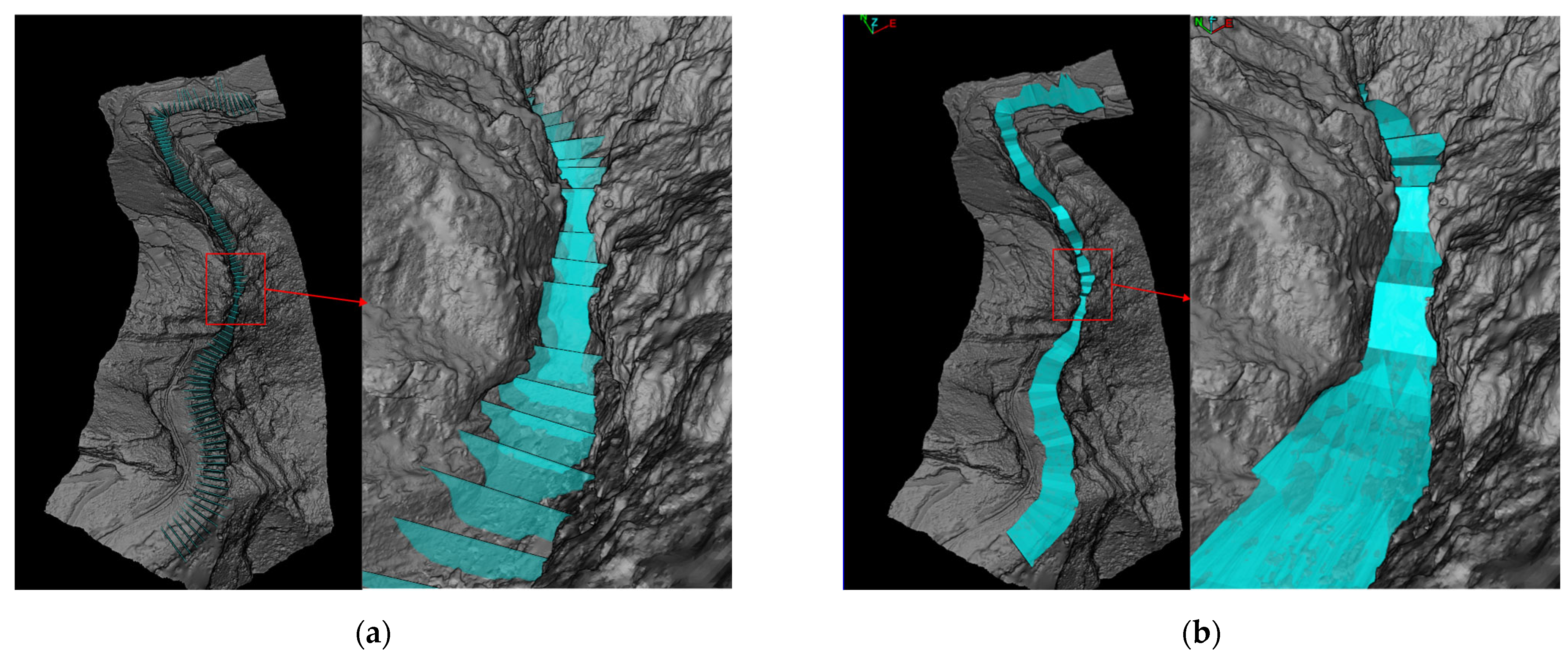
Finally, Figure 13 provides 3D visualizations of the mesh with the simulated water levels. This realistic representation is a valuable tool for planning infrastructure, such as tourist boardwalks, by accurately identifying flood hazards in complex 3D environments.
Figure 13.
Views of water height level reached in this study: (a) cross-sections; (b) stream surface.
4. Discussion
Modeling narrow gorges and canyons using geomatic techniques is a complex task due to several factors. The primary challenge is the narrow geometry, which obstructs views from both the exterior and the interior. This circumstance makes it impossible to use GNSS within these environments due to the lack of satellite signals. Additionally, classical surveying techniques (e.g., total station) are often unviable due to the requirement for stable topographic points and the presence of occlusions that impede line-of-sight. Furthermore, the common presence of water and dense vegetation at the bottom of these scenes complicates data acquisition. While aerial techniques (LiDAR and photogrammetry) are standard for obtaining DTMs globally, they often fail to achieve a comprehensive and realistic geometry in narrow areas due to the lack of visibility from aerial nadir views, as demonstrated by the results of DTM3. Similarly, the exclusive use of terrestrial techniques does not guarantee a realistic terrain model, as the higher areas of the canyon are usually hidden from the bottom. Consequently, these environments cannot be accurately modeled using a single technique; a multi-sensor approach is essential.
In this study, we integrated multiple aerial and terrestrial techniques to overcome these issues. The results demonstrate the viability of the proposed methodology for documenting narrow canyons. Data fusion is fundamental in these cases to achieve a comprehensive terrain model and to facilitate the use of specific techniques that would otherwise be non-viable if used individually. The application of our approach highlights several critical aspects:
- Georeferencing: The challenges of establishing a CRS in narrow or inaccessible spaces can be overcome by employing aerial LiDAR and photogrammetry. These techniques allow for the determination of GCPs and CPs that provide the necessary spatial control to support terrestrial techniques.
- Geometry: The determination of geometry based on TLS, supported by MMS and aerial LiDAR, yielded good results, providing a complete 3D mesh even in extremely difficult cases characterized by occlusions or inaccessibility. TLS allows for high relative accuracy inside the canyon; drift errors are limited to those occurring during the registration process and can be reduced by ensuring large overlaps between adjacent point clouds. The high resolution of TLS point clouds allows for the identification of GCPs to be georeferenced against aerial data and subsequently used for other datasets (e.g., SP). However, the disadvantage of static TLS is the existence of unavoidable occlusions, even with numerous stations. This limitation is addressed by using mobile techniques (LiDAR or videogrammetry). Once the final point cloud is obtained, semi-automatic classification to discriminate terrain versus non-terrain data effectively determines a complete mesh, including areas with inverted topography. LiDAR data remains fundamental for defining the terrain in areas with dense vegetation where photogrammetric techniques often fail.
- Texture: The texture obtained through photogrammetric techniques (aerial and terrestrial) enabled the creation of a comprehensive 3D model with a realistic appearance. Spherical Photogrammetry (SP) proved to be an excellent technique to supplement aerial imagery due to its high data acquisition efficiency in narrow areas. Moreover, the determination of extrinsic parameters following a complete calibration of the 360-degree camera streamlines the orientation process, reducing the number of GCPs needed. While SP could also be used to determine geometry, one must consider the inherent difficulties of image-based methods in the presence of dense vegetation.
Regarding the canyon geometry based on the 3D model and the DTMs, several conclusions can be drawn:
- Our approach, based on the high-fidelity representation provided by a 3D mesh, constitutes the optimal option for analyzing these narrow areas because it represents the geometric reality, representing the riverbed, overhangs and inverted topography correctly.
- DTMs obtained from 3DM showed reliable results only in open areas where inverted topography is negligible. DTMs that use maximum elevation points (top-view, DTM1) retain these points while removing the bottom geometry and inverted topography, effectively raising the riverbed and narrowing the canyon. Conversely, DTMs using minimum elevation points (bottom-view, DTM2) remove overhangs, which widens the cross-sections while maintaining the riverbed elevation.
- Publicly available DTMs (DTM3) based on aerial LiDAR often lack data from the interior areas of the canyon, leading to a loss of bottom geometry and narrowing of the cross-sections, yielding results similar to DTM1.
- If 2.5D terrain models must be used, we recommend DTMs obtained using minimum elevation points (bottom-view, DTM2), provided they are derived from a previously established 3D model to ensure the inclusion of the true riverbed.
Finally, the analysis of water height and flow velocity led to the following observations:
- In open areas, the results of using 3D and 2.5D terrain models are quite similar.
- In narrow areas, the results depend heavily on the terrain model used. The 3DM, representing the comprehensive geometry, consistently shows the most realistic results. Standard DTMs result in significant overestimation or underestimation of the water height. In general, DTM1 and DTM3 overestimate water height and underestimate flow velocity. On the contrary, DTM2 underestimates water height and overestimates flow velocity, although to a lesser degree.
- Due to the calculation direction (downstream to upstream), discrepancies caused in narrow areas are translated to subsequent open areas.
- We recommend the use of 3D models for hydraulic modelling. However, if 2.5D terrain models are required, we recommend DTMs obtained using minimum elevation points (bottom-view, DTM2), as their results are more aligned with the 3D model, provided the aforementioned issues in narrow areas are considered.
Despite the success of this approach, some limitations must be considered for future work. The presence of extremely dense vegetation, the logistical necessity of capturing data from the river, and the difficulty of identifying GCPs in certain spots can limit applicability. Therefore, adaptations must be considered to overcome these specific challenges in other cases.
5. Conclusions
This study has presented a novel approach to the comprehensive modelling of narrow gorges and canyons, overcoming the inherent difficulties of these environments. Consequently, accurate modelling in these scenes is unfeasible without the integration of multiple techniques and robust data fusion. This fusion is essential not only for ensuring data completion but also for enabling the use of sensors that cannot operate individually in such constrained spaces and for establishing a reliable georeferencing framework.
The primary conclusions reflecting the novelty of this study include the following:
- Georeferencing strategy based on UAV-RTK data as a basis for previously registered TLS point clouds
- Terrestrial synergy: While exterior areas are effectively captured via aerial techniques, interior documentation relies on the synergy between TLS and MMS. TLS provides the necessary geometric accuracy, while MMS facilitates the completion of the model by reaching occluded areas.
- Visual Fidelity: Spherical Photogrammetry (SP) is identified as the most efficient image-based technique for capturing visual data in narrow interiors.
- Hydraulic Implications: The analysis of cross-sections confirms that a 3D mesh, unlike traditional DTMs, provides more realistic water height levels in canyons. This has important implications for flood risk assessment, hydraulic modelling, civil protection and emergency management, and infrastructure resilience planning. In the case of using DTMs, we recommend the use of minimum elevation points (bottom-view) from a 3D mesh.
Although high-resolution 3D models are currently computationally intensive for large-scale applications based on computational fluid dynamics, this study represents a significant first step by providing a comprehensive model that accurately reflects the complex behavior of canyon terrain.
Future work will focus on optimizing data capture and processing. Potential research lines include the following:
- Integrating 360-degree cameras directly onto UAV platforms.
- Improving MMS capture protocols and drift-correction algorithms to enhance accuracy further.
- Incorporating bathymetric techniques to account for river depth in cases where water volume is significant.
- Applying the high-fidelity 3D geometry obtained here to more complex hydrodynamic models will further refine the simulation of water behavior in high-risk environments.
Author Contributions
Conceptualization, J.L.P.-G., J.M.G.-L., A.T.M.-C. and D.V.-G.; methodology, J.L.P.-G., J.M.G.-L., A.T.M.-C. and D.V.-G.; software, J.L.P.-G., J.M.G.-L., A.T.M.-C. and D.V.-G.; validation, J.L.P.-G., J.M.G.-L., A.T.M.-C. and D.V.-G.; formal analysis, J.L.P.-G., J.M.G.-L., A.T.M.-C. and D.V.-G.; investigation, J.L.P.-G., J.M.G.-L., A.T.M.-C. and D.V.-G.; resources, J.L.P.-G., J.M.G.-L., A.T.M.-C. and D.V.-G.; data curation, J.L.P.-G., J.M.G.-L., A.T.M.-C. and D.V.-G.; writing—original draft preparation, A.T.M.-C.; writing—review and editing, J.L.P.-G., J.M.G.-L., A.T.M.-C. and D.V.-G.; visualization, J.L.P.-G., J.M.G.-L., A.T.M.-C. and D.V.-G.; supervision, J.L.P.-G., J.M.G.-L., A.T.M.-C. and D.V.-G.; project administration, J.L.P.-G. All authors have read and agreed to the published version of the manuscript.
Funding
This research received no external funding.
Data Availability Statement
The data presented in this study are available on request from the corresponding author. The data are not publicly available due to privacy restrictions.
Acknowledgments
The authors would like to thank the CEACTEMA (University of Jaén) for its resources. During the preparation of this manuscript/study, the authors used Gemini v. 2.5 for the purposes of English style checking. The authors have reviewed and edited the output and take full responsibility for the content of this publication.
Conflicts of Interest
The authors declare no conflicts of interest.
Abbreviations
The following abbreviations are used in this manuscript:
| 3DM | 3D Mesh |
| ASML | Above sea mean level |
| CP | Check Point |
| CRS | Coordinate Reference System |
| DSM | Digital Surface Model |
| DTM | Digital Terrain Model |
| GCP | Ground Control Point |
| GNSS | Global Navigation Satellite System |
| ICP | Iterative Closest Point |
| IGN | National Geographic Institute (Spain) |
| LiDAR | Light Detection and Ranging |
| MMS | Mobile Mapping System |
| MTN | National Topographic Map (Spain) |
| MVS | Multi-View Stereo |
| PNOA | National Plan for Aerial Orthophotography (Spain) |
| RMSE | Root Mean Square Error |
| RTK | Real-Time Kinematic |
| SfM | Structure from Motion |
| SLAM | Simultaneous Localization and Mapping |
| SP | Spherical Photogrammetry |
| TLS | Terrestrial Laser Scanner |
| UAV | Unmanned Aerial Vehicle |
Appendix A
Table A1.
Sensors used in this study.
References
- Hungr, O.; Leroueil, S.; Picarelli, L. The Varnes classification of landslide types, an update. Landslides 2014, 11, 167–194. [Google Scholar] [CrossRef] [Scilit]
- Borga, M.; Stoffel, M.; Marchi, L.; Marra, F.; Jakob, M. Hydrogeomorphic response to extreme rainfall in headwater systems: Flash floods and debris flows. J. Hydrol. 2014, 518, 194–205. [Google Scholar] [CrossRef] [Scilit]
- Žabota, B.; Repe, B.; Kobal, M. Influence of digital elevation model resolution on rockfall modelling. Geomorphology 2019, 328, 183–195. [Google Scholar] [CrossRef] [Scilit]
- Griffiths, P.G.; Webb, R.H.; Melis, T.S. Frequency and initiation of debris flows in Grand Canyon, Arizona. J. Geophys. Res. Earth Surf. 2004, 109, F04002. [Google Scholar] [CrossRef] [Scilit]
- Iverson, R.M. The Physics of Debris Flows. Rev. Geophys. 1997, 35, 245–296. [Google Scholar] [CrossRef] [Scilit]
- Wohl, E. Mountain Rivers Revisited; John Wiley & Sons: Hoboken, NJ, USA, 2013; Volume 19. [Google Scholar]
- Qi, W.; Ma, C.; Xu, H.; Chen, Z.; Zhao, K.; Han, H. A Review on Applications of Urban Flood Models in Flood Mitigation Strategies. Nat. Hazards 2021, 108, 31–62. [Google Scholar] [CrossRef] [Scilit]
- Shen, Y.; Jiang, C. A comprehensive review of watershed flood simulation model. Nat. Hazards 2023, 118, 875–902. [Google Scholar] [CrossRef] [Scilit]
- Flood Simulation in ArcGIS Pro 3.6, ESRI. Available online: https://www.esri.com/content/dam/esrisites/en-us/media/technical-papers/flood-simulation-arcgis-pro.pdf (accessed on 24 December 2025).
- Hydrologic Engineering Center. US Army Corps of Engineers. Available online: https://www.hec.usace.army.mil/ (accessed on 24 December 2025).
- Pinos, J.; Timbe, L. Performance assessment of two-dimensional hydraulic models for generation of flood inundation maps in mountain river basins. Water Sci. Eng. 2019, 12, 11–18. [Google Scholar] [CrossRef] [Scilit]
- Kumar, V.; Azamathulla, H.M.; Sharma, K.V.; Mehta, D.J.; Maharaj, K.T. The State of the Art in Deep Learning Applications, Challenges, and Future Prospects: A Comprehensive Review of Flood Forecasting and Management. Sustainability 2023, 15, 10543. [Google Scholar] [CrossRef] [Scilit]
- Flow-3D Hydro, the Complete 3D CFD Modeling Solution. Available online: https://www.flow3d.com/products/flow-3d-hydro/ (accessed on 24 December 2025).
- Kovanič, Ľ.; Topitzer, B.; Peťovský, P.; Blišťan, P.; Gergeľová, M.B.; Blišťanová, M. Review of photogrammetric and lidar applications of UAV. Appl. Sci. 2023, 13, 6732. [Google Scholar] [CrossRef] [Scilit]
- Vélez-Nicolás, M.; García-López, S.; Barbero, L.; Ruiz-Ortiz, V.; Sánchez-Bellón, Á. Applications of Unmanned Aerial Systems (UASs) in Hydrology: A Review. Remote Sens. 2021, 13, 1359. [Google Scholar] [CrossRef] [Scilit]
- Iqbal, U.; Riaz, M.Z.B.; Zhao, J.; Barthelemy, J.; Perez, P. Drones for Flood Monitoring, Mapping and Detection: A Bibliometric Review. Drones 2023, 7, 32. [Google Scholar] [CrossRef] [Scilit]
- Lichti, D.D.; Tredoux, W.; Maalek, R.; Helmholz, P.; Radovanovic, R. Modelling extreme wide-angle lens cameras. Photogramm. Rec. 2021, 36, 360–380. [Google Scholar] [CrossRef] [Scilit]
- Fangi, G.; Nardinocchi, C. Photogrammetric processing of spherical Panoramas. Photogramm. Rec. 2013, 28, 293–311. [Google Scholar] [CrossRef] [Scilit]
- Di Stefano, F.; Chiappini, S.; Gorreja, A.; Balestra, M.; Pierdicca, R. Mobile 3D scan LiDAR: A literature review. Geomat. Nat. Hazards Risk 2021, 12, 2387–2429. [Google Scholar] [CrossRef] [Scilit]
- Elhashash, M.; Albanwan, H.; Qin, R. A Review of Mobile Mapping Systems: From Sensors to Applications. Sensors 2022, 22, 4262. [Google Scholar] [CrossRef] [Scilit]
- Ullman, S. The interpretation of structure from motion. Proc. Royal Soc. B 1979, 203, 405–426. [Google Scholar]
- Lowe, D.G. Distinctive image features from scale-invariant keypoints. Int. J. Comput. Vis. 2004, 60, 91–110. [Google Scholar] [CrossRef] [Scilit]
- Seitz, S.M.; Curless, B.; Diebel, J.; Scharstein, D.; Szeliski, R. A comparison and evaluation of multi-view stereo reconstruction algorithms. In Proceedings of the 2006 IEEE Computer Society Conference on Computer Vision and Pattern Recognition, New York, NY, USA, 17–22 June 2006. [Google Scholar]
- Furukawa, Y.; Hernández, C. Multi-view stereo: A tutorial. Found. Trends Comput. Graph. Vis. 2015, 9, 1–148. [Google Scholar] [CrossRef] [Scilit]
- Zhang, Z. Iterative closest point (ICP). In Computer Vision: A Reference Guide, 1st ed.; Ikeuchi, K., Ed.; Springer International Publishing: Cham, Switzerland, 2021; pp. 718–720. [Google Scholar]
- Agisoft Metashape. Available online: https://www.agisoft.com/ (accessed on 24 December 2025).
- CloudCompare. Open Source Project. Available online: https://www.cloudcompare.org/ (accessed on 24 December 2025).
- Muhadi, N.A.; Abdullah, A.F.; Bejo, S.K.; Mahadi, M.R.; Mijic, A. The Use of LiDAR-Derived DEM in Flood Applications: A Review. Remote Sens. 2020, 12, 2308. [Google Scholar] [CrossRef] [Scilit]
- Samadzadegan, F.; Toosi, A.; Dadrass Javan, F. A critical review on multi-sensor and multi-platform remote sensing data fusion approaches: Current status and prospects. Int. J. Remote Sens. 2024, 46, 1327–1402. [Google Scholar] [CrossRef] [Scilit]
- Destefanis, T.; Guliyeva, S.; Boccardo, P.; Fissore, V. Advancing Flood Detection and Mapping: A Review of Earth Observation Services, 3D Data Integration, and AI-Based Techniques. Remote Sens. 2025, 17, 2943. [Google Scholar] [CrossRef] [Scilit]
- Pérez-García, J.L.; Mozas-Calvache, A.T.; Gómez-López, J.M.; Vico-García, D.; Delgado-García, J. Multi-Technique 3D Modelling of Narrow Gorges to Assess Stability: Case Study of Caminito Del Rey (Spain). Remote Sens. 2025, 17, 3702. [Google Scholar] [CrossRef] [Scilit]
- Pérez-García, J.L.; Gómez-López, J.M.; Mozas-Calvache, A.T.; Delgado-García, J. Analysis of the Photogrammetric Use of 360-Degree Cameras in Complex Heritage-Related Scenes: Case of the Necropolis of Qubbet el-Hawa (Aswan Egypt). Sensors 2024, 24, 2268. [Google Scholar] [CrossRef] [Scilit] [PubMed]
- Chow, V.T.; Maidment, D.R.; Mays, L.W. Applied Hydrology; McGraw-Hill: New York, NY, USA, 1988; p. 572. [Google Scholar]
- Chaudhry, M.H. Computation of gradually varied flow. In Open-Channel Flow, 3rd ed.; Springer International Publishing: Cham, Switzerland, 2008; pp. 155–201. [Google Scholar]
- HEC-RAS Hydraulic Reference Manual. Available online: https://www.hec.usace.army.mil/confluence/rasdocs/ras1dtechref/6.5 (accessed on 24 December 2025).
- Arroyo, R.M.S.; Martínez, J.D.S. La transformación de las cuencas de los ríos Eliche y Jaén en un territorio-riesgo: Dinámica y perspectivas. Nimbus Rev. Climatol. Meteorol. Paisaje 2012, 29-30, 643–658. [Google Scholar]
- Gómez-López, J.M.; Pérez-García, J.L.; Mozas-Calvache, A.T.; Delgado-García, J. Mission Flight Planning of RPAS for Photogrammetric Studies in Complex Scenes. ISPRS Int. J. Geo-Inf. 2020, 9, 392. [Google Scholar] [CrossRef] [Scilit]
- DJI Terra—DJI Enterprise. Available online: https://enterprise.dji.com/dji-terra (accessed on 24 December 2025).
- BayesStripAlign: LiDAR Strip Adjustment and Calibration. Available online: https://bayesmap.com/products/bayesstripalign/ (accessed on 24 December 2025).
- Maptek—Point Cloud Processing & Analasys. Available online: https://www.maptek.com/products/pointstudio/ (accessed on 24 December 2025).
- Overview of All Lastools—Rapidlasso GmbH. Available online: https://rapidlasso.de/product-overview/ (accessed on 24 December 2025).

Disclaimer/Publisher’s Note: The statements, opinions and data contained in all publications are solely those of the individual author(s) and contributor(s) and not of MDPI and/or the editor(s). MDPI and/or the editor(s) disclaim responsibility for any injury to people or property resulting from any ideas, methods, instructions or products referred to in the content. |
© 2026 by the authors. Licensee MDPI, Basel, Switzerland. This article is an open access article distributed under the terms and conditions of the Creative Commons Attribution (CC BY) license.