


Abstract
In natural scenes, the high resemblance between unripe tomatoes and foliage, combined with severe occlusion, challenges current semantic segmentation models, causing poor accuracy and indistinct boundaries. To overcome this, we propose CMAE-UNet, a camouflage suppression and edge enhancement model based on the UNet architecture. Specifically, a Global-Local Integrated Spatial Attention (GLISA) encoder merges dual-branch dilated convolutions, residual structures, and an Efficient Multi-scale Attention mechanism to expand receptive fields and highlight targets in complex backgrounds. Furthermore, a Frequency-Domain Feature Enhancement (FFE) module leverages the Fast Fourier Transform to separate and adaptively enhance distinct frequency components, effectively mitigating camouflage interference. Additionally, a Directional Edge Enhancement (DEE) module uses three-directional learnable convolutions and spatial attention to sharpen indistinct target contours. Evaluated on a custom Tomato dataset encompassing five complex scenarios, CMAE-UNet outperforms 12 prominent methods in mIoU, Dice, and Sen metrics, yielding smoother and more precise segmentation boundaries. The model robustly withstands field interference, providing strong technological support for automated tomato detection, intelligent harvesting, and growth monitoring.
1. Introduction
In the context of the global shift towards smart agriculture, high-resolution image processing for orchard segmentation and AI-driven fruit recognition have emerged as fundamental technologies for precision management, enabling automated harvesting, accurate yield forecasting, and early disease detection. Currently, fruit image segmentation has been extensively studied across various crops. For example, Liu et al. [1] proposed an instance segmentation method for accurate cucumber detection in complex greenhouse environments; Shen et al. [2] proposed an improved Mask R-CNN model to achieve precise instance segmentation of grape clusters in the field; Wang et al. [3] proposed a lightweight Mask R-CNN algorithm to achieve precise and rapid segmentation of individual strawberries; Han et al. [4] proposed the SSW-YOLOv11n lightweight model to improve apple segmentation accuracy and inference efficiency; Yang et al. [5] proposed the LitchiPhenoNet multimodal framework to address the challenges of lychee segmentation; Wang et al. [6] achieved accurate segmentation and recognition of camellia fruit based on Mask-RCNN; and Hu et al. [7] proposed a U-Net model integrating PDE and GCN to achieve precise segmentation of sweet cherries. Furthermore, to address more complex visual challenges, Evangelista et al. [8] introduced the FCNet Transformer segmentation framework, successfully attaining precise segmentation of camouflaged mangoes in agricultural settings, while Wen et al. [9] introduced the SCAL multi-class instance segmentation model, improving the efficacy of visual solutions for intelligent harvesting in intricate situations. Despite these advances, the specific detection of green fruits and immature targets—which blend seamlessly with canopy backgrounds—remains insufficiently explored.
Research in tomato image segmentation demonstrates that ripe tomatoes are easily identifiable in images owing to their vivid red-green colour contrast and distinct textural characteristics, rendering them a prominent topic in the visual recognition of fruits and vegetables [10]. Wei et al. [11] introduced the enhanced ACP-Tomato-Seg algorithm, which proficiently tackles the issue of precisely segmenting ripe tomatoes in intricate field conditions. Dubey et al. [12] created TomatoRipen-MMT, an RGB-NIR multispectral fusion model utilising the Transformer architecture, which attained high-precision identification of ripe tomatoes in intricate greenhouse settings. Ai et al. [13] introduced the DLQM enhanced segmentation model derived from YOLOv11n. By enhancing and optimising the multi-branch feature and the lightweight detecting head, they effectively resolved the challenges of dense occlusion of ripe tomato clusters in greenhouses, difficulty in precise segmentation, and the disparity between model correctness and real-time performance. Minagawa et al. [14] employed a Mask R-CNN network to identify tomato clusters and assess ripeness, allowing accurate predictions of harvest timing for individual tomatoes and significantly enhancing the flexibility of intelligent tomato harvesting in agricultural settings. A summary of these previous studies reveals their primary limitation: current tomato segmentation algorithms heavily rely on prominent color contrasts and are explicitly tailored for ripe fruits. Consequently, they often struggle when applied to unripe tomatoes, which display subtle visual traits, lack sufficient color distinction, and blend significantly with the green backdrop.
The segmentation of unripe tomatoes presents distinct technical hurdles compared to ripe fruits or standard camouflaged object detection. Unripe tomatoes exhibit a consistent greenish-yellow coloration that closely resembles surrounding leaves and weeds, creating a homogeneous camouflage [15]. Furthermore, their indistinct edges and subtle contour gradients make feature extraction highly challenging. This research faces two primary difficulties: first, the analogous hues of fruit and vegetation cause optical concealment, while irregular size distributions complicate edge refinement and localization [16]; second, severe obstruction by branches and foliage obscures beneficial characteristics, leading to false negatives and blurred fruit-foliage boundaries [17,18].
To address these issues, this paper presents an enhanced semantic segmentation model, CMAE-UNet, based on the UNet architecture. This paradigm relies on three synergistic components: the Global-Local Integrated Spatial Attention (GLISA) module, designed to adaptively calibrate features to maintain stable target representations; the Frequency-Domain Feature Enhancement (FFE) module, which utilizes frequency decomposition with the goal of decoupling camouflaged targets, mitigating noise, and enhancing multi-scale fusion; and the Directional Edge Enhancement (DEE) module, which employs three-directional learnable convolutions aimed at restoring contour details and reducing occlusion-driven feature loss. Working collaboratively, these modules are expected to achieve superior segmentation proficiency under intricate field conditions.
Therefore, the overarching objective of this study is to develop an effective and reliable semantic segmentation algorithm capable of overcoming the severe “green-on-green” camouflage and occlusion challenges inherent in unripe tomato detection, thereby providing dependable visual perception for intelligent agricultural harvesting systems. To achieve this objective, the primary contributions of this work are threefold. Initially, we developed a multi-scenario dataset of unripe tomatoes (ZKMTD) comprising 1254 smartphone images split into a training (878) and testing (376) set at a 7:3 ratio. The dataset replicates robot vision across diverse field conditions, including variable illumination, dense occlusions, and multi-perspective views, with precise annotations outlining even obscured fruits. Subsequently, the CMAE-UNet model was proposed, integrating the GLISA, FFE, and DEE modules to robustly segment camouflaged targets. Lastly, systematic experimental validation demonstrated that CMAE-UNet outperforms 12 prominent segmentation models across three fundamental metrics: mIoU, Dice, and Sen, while ablation studies confirmed the efficacy of each innovative module.
2. Related Work
2.1. Fruit Image Segmentation
Fruit image segmentation is a fundamental technique in agricultural visual perception and intelligent harvesting. The primary challenge is achieving pixel-level accuracy for fruit segmentation and contour extraction in complex open-field environments, where factors like varying illumination, foliage occlusion, fruit clustering, and immature fruit camouflage substantially degrade precision. Current research primarily focuses on model architecture optimization and learning paradigm innovations, both offering valuable insights for unripe tomato segmentation.
Research in architectural optimization concentrates on enhancing environmental adaptability. Wu et al. [19] introduced SemIns-YOLOv8, integrating a semantic segmentation module, a joint loss function, and boundary enhancement for real-time cherry segmentation. Liu et al. [20] combined U-Net mask extraction with elliptical fitting to resolve occlusion in trellised watermelons. Luo et al. [21] improved YOLO11n-Seg using SCA and DAB modules alongside the NWD metric to enhance occlusion resilience for greenhouse blueberries. Yang et al. [22] integrated NeRF with RandLA-Net to generate fruit point clouds, boosting citrus IoU by 7.33%. Furthermore, Xu et al. [23] proposed RSA-YOLOv8s for multi-fruit segmentation; Wang et al. [24] developed MS-ADS to tackle apple segmentation; and Li et al. [25] upgraded Deeplabv3+ with PSA and SP modules to augment fruit tree segmentation.
Innovations in learning paradigms address data scarcity and poor model generalization in agricultural vision. For instance, James et al. [26] introduced a transfer learning framework for few-shot fruit segmentation, enabling field segmentation using minimal labeled images. Furthermore, to combat the high cost of pixel-level annotation in complex environments, researchers have explored alternative learning strategies. For example, Barth et al. [27] demonstrated the efficacy of using synthesized agricultural image datasets (data synthesis) to pre-train segmentation models, significantly reducing manual labeling efforts. Additionally, weakly-supervised and semi-supervised learning paradigms [28] have been increasingly adopted to leverage vast amounts of unannotated orchard data, directly improving the generalization capabilities of segmentation models in unseen field scenarios.
In conclusion, while existing models effectively address occlusion, overlap, and lighting interference for ripe fruits, they generally lack sufficient adaptability for highly complex scenes. Building on prior techniques—such as module optimization, multi-feature fusion, and few-shot learning—this study departs from the standard optimization logic tailored for ripe fruits. To address the weak features and strong camouflage of unripe tomatoes, we propose a specialized segmentation network and training strategy designed explicitly for complex, homogeneous backdrops.
2.2. Anti-Interference Technology for Camouflage Suppression in Complex Backgrounds
In visual segmentation, high color and texture similarity between targets and backgrounds creates severe camouflage interference, often causing models to generate false positives and negatives. Addressing this is crucial for robust real-world segmentation. Li et al. [29] proposed a difference-aware decoder that uses a two-branch, three-stage architecture to generate guidance maps and background-aware features, thereby amplifying the differences between foreground and background and improving binary segmentation accuracy in complex backgrounds. He et al. [30] introduced the FEDER model, which uses learnable wavelets for frequency-domain feature decomposition and combines frequency attention with a differential equation-inspired edge reconstruction module to differentiate camouflaged objects from complicated backgrounds. Yin et al. [31] created CamoFormer, which uses Mask-Separable Attention (MSA) to identify camouflaged objects from the backdrop using a multi-mask method, and combines it with a top-down decoder to accomplish high-precision camouflage identification. Sun et al. [32] presented CamoDiffusion, a method that iteratively refines the borders of camouflaged objects and reduces misclassifications in high-uncertainty locations. Yang et al. [33] introduced UGDNet, which explicitly captures prediction uncertainty and uses it as an anchor to direct the diffusion process, improving the robustness of disguised object recognition against interference. Zhang et al. [34] created CGNet, which uses class-prior information to create a class-guided camouflaged object identification framework, therefore increasing object perception stability in complicated environments. Lei et al. [35] introduced ConDSeg, which separates the foreground, background, and doubtful areas in medical pictures by decoupling semantic information and combining contrast-driven feature aggregation.
While effective in general and medical imagery, current camouflage suppression methods struggle to adapt to the uniform camouflage environments unique to the agricultural sector. Specifically, generic models are primarily optimized for isolated entities. They struggle with the dense clustering and severe foreground occlusion by identical-colored stems and leaves—a distinct feature of unripe tomatoes. Furthermore, heavy architectures like diffusion models or Transformers incur prohibitive computational costs for agricultural applications. Building upon established techniques like feature decoupling, uncertainty modeling, and frequency-domain enhancement, this study develops specialized background suppression and contour restoration mechanisms explicitly tailored to the specific camouflage traits of unripe tomatoes.
2.3. Edge Contour Refinement Technology
Field conditions such as foliage occlusion, overlapping fruits, and adverse lighting (shadows, low contrast) often cause edge discontinuities, contour distortion, and blurred boundaries, severely degrading segmentation accuracy. Therefore, targeted edge optimization and contour reconstruction are crucial for robust real-world segmentation. Huang et al. [36] proposed MSEONet, integrating MSCA, CEE, and EPFO modules to resolve undersampled edges and improve boundary accuracy in remote sensing images. Yu et al. [37] introduced PEEN, utilizing a probability function, convolutional self-attention, and iterative optimization to successfully segment weak edges and occluded objects. Wang et al. [38] developed ContourMS, framing medical segmentation as a contour regression task to reconstruct blurred boundaries via coarse mask prediction and expert-level refinement. He et al. [30] incorporated edge reconstruction into FEDER, using a differential equation module to precisely delineate camouflaged object borders. Zhang et al. [39] presented ACFA and TFFA modules to enhance the capture of edges, textures, and spatial structures via tri-directional attention and tri-domain feature fusion.
Although existing edge optimization techniques have significantly improved the quality of edge segmentation in remote sensing, medical, and conventional camouflaged images, their applicability in agricultural scenarios is clearly limited. This study departs from traditional edge optimization methods and proposes an iterative edge refinement and boundary detection strategy tailored to the characteristics of unripe tomatoes, which feature weak edge gradients and highly concealed edges. The method focuses on capturing subtle contour changes against a homogeneous background, thereby achieving accurate and complete reconstruction of the fruit edges.
3. Collection and Construction of Dataset
3.1. Data Construction
The tomato dataset included in this study was gathered from an open-air rooftop cultivation system at Zhongkai University of Agricultural Engineering’s Haizhu Campus. To accurately describe the growing environment, the tomatoes (a standard commercial cultivar, Solanum lycopersicum L.) were cultivated in soil-based raised beds arranged in rows. The plants were grown under natural conditions without any greenhouse, canopy, or protective structures. Standard open-field agronomic management practices were applied. This open-air setup directly exposes the plants to natural weather and sunlight variations, authentically replicating the complex illumination, shading, and background interference typically encountered in open agricultural environments. A smartphone was employed as the image capturing device to align more closely with practical robotic applications, since its resolution is better suitable for the real-time processing requirements of robotic vision systems and effectively mitigates the computational expenses linked to high-resolution data. Throughout data collection, the camera angle, distance, and composition were adjusted to encompass a broad spectrum of fruit shapes and field backgrounds, ensuring data variety. After manual screening, 1254 genuine photographs were obtained and employed to develop the “Zhongkai Multi-scenario Tomato Image Dataset (ZKMTD). The training dataset has 878 photographs, whereas the test dataset contains 376 pictures. Figure 1 and Figure 2 present examples of standard unripe tomato images from many situations within this collection. The ZKMTD exhibits both diversity and practicality in scenario design, fruit form, and surrounding backdrops. This aligns with the characteristics of robotic harvesting and offers data support that accurately meets practical requirements for training, verifying, and testing the CMAE-UNet model.
Figure 1.
Partial view of the ambient lighting scene dataset. Panels (a–c) depict standard lighting condition. Panels (d–f) illustrate low lighting conditions.
Figure 2.
Partial view of the dataset for complex technical challenge scenarios. (a–c) depict complex occlusion situations. (d–f) depict a combination of near-field and far-field contexts. (g–i) depict Dense, highly analogous scenes.
The first group encompasses ambient illumination situations. Figure 1 illustrates: a–c depict standard lighting conditions, featuring uniform illumination and high image clarity, typical of daytime field operations; d–f illustrate low lighting conditions, marked by diminished brightness and contrast, emulating challenging lighting scenarios such as overcast skies, backlighting within greenhouses, and low light during dawn or dusk. The two categories of lighting samples complement one another, effectively mitigating the segmentation challenges posed by unstable field lighting and abrupt variations in brightness, and are employed to assess the algorithm’s adaptive anti-interference capability in response to fluctuations in light intensity.
The second category encompasses scenes featuring intricate targets and technical obstacles, concentrating on the classification and organization of unripe tomatoes according to their inherent segmentation difficulties. As illustrated in Figure 2a–c depict complex occlusion situations, including common interferences such as entangled branches and leaves, partially obscured fruits, and cluttered backdrops; d–f illustrate a combination of near-field and far-field contexts, where near-field fruits are distinctly visible. This precisely reflects the imaging disparity encountered in field photography—where proximal objects are in focus while distant ones appear blurred—mimicking the segmentation difficulties arising from this gradient of sharpness; g–i Dense, highly analogous scenes in which the colours and textures of the fruits and adjacent foliage significantly overlap, leading to substantial interference from uniform texture camouflage. This collection of situations effectively addresses the primary technological challenges previously outlined, including severe occlusion, significant variations in image clarity, and restricted target-background differentiation.
3.2. Data Preparation
The dataset was labelled using LabelMe. Throughout the annotation process, even when fruits were obscured by branches and foliage or only partially visible, the discernible regions were accurately demarcated to ensure the annotations were thorough and subsequent model training was efficient. Figure 3 illustrates the original photographs with their corresponding annotated versions:
Figure 3.
Partial view of the dataset; (a) original image, (b) annotation mask.
4. Research Methodology and Model Design
4.1. Semantic Segmentation Model U-Net
U-Net [40] is a classic deep learning network that has been widely adopted in the field of image segmentation. Its overall structure is shown in Figure 4, with its core consisting of two major modules working in tandem: the encoder’s downsampling branch and the decoder’s upsampling branch. The encoder relies on sequential convolutional operations and pooling for dimensionality reduction to progressively extract and aggregate deep contextual features from the image; the decoder, on the other hand, uses deconvolution and upsampling to progressively restore the original spatial dimensions of the feature maps and reconstruct the detailed edge information of the target. The most prominent feature of this network is the addition of a cross-layer skip connection mechanism, which efficiently fuses high-resolution, detailed features from shallow layers with global semantic features from deep layers. This significantly enhances the model’s ability to capture target contour edges and substantially improves pixel-level segmentation accuracy.
Figure 4.
U-Net Model Architecture [40].
The reason this study selected U-Net as the underlying architecture was based on a comprehensive consideration of the perception requirements for complex camouflaged scenes and the practical hardware constraints of agricultural robot deployments. Although modern complex Transformer-based network architectures (such as SAM and CamoFormer) have demonstrated certain advantages in global feature representation and the processing of camouflaged targets in recent years, their excessive number of parameters and extremely high inference latency make it difficult to meet real-time operational requirements on computationally constrained agricultural edge embedded devices. In contrast, U-Net not only maintains a relatively lightweight network size (beneficial for edge deployment), but its cross-layer feature fusion mechanism also provides a solid foundation for capturing the faint edge contours of unripe tomatoes. Therefore, this study uses U-Net as its foundation and specifically introduces camouflage suppression and edge enhancement modules. This design avoids the massive computational overhead associated with Transformer architectures and successfully strikes a balance between “computational cost” and “complex scene perception capabilities.”
4.2. CMAE-UNet Model Architecture
CMAE-UNet is a segmentation model for immature tomatoes that is specifically designed for complex field scenarios. It is based on the UNet architecture and comprises three main modules, as illustrated in Figure 5 (which comprehensively details the spatial resolutions and channel dimensions at every stage). Initially, we suggest that the Global-Local Integrated Spatial Attention (GLISA) module serve as the fundamental component across all levels of both the encoder and decoder. The receptive field is expanded while fine-grained features are preserved by combining dual-branch dilated convolutions with a residual structure in this module. It also integrates Efficient Multi-scale Attention (EMA) to improve the model’s capacity to perceive tomato features in settings with varying object scales and uneven illumination by enhancing features across both spatial and channel dimensions. Secondly, this paper introduces a Frequency Domain Feature Enhancement (FFE) module, which is systematically applied across all five levels along the skip connections and the bottleneck, to reduce camouflage interference induced by similar backgrounds. In order to enhance the model’s capacity to decouple features of camouflaged objects, this module employs the Fast Fourier Transform (FFT) to decompose features into low-, mid-, and high-frequency components for adaptive enhancement. This process integrates global structure, texture, and edge details. Lastly, this paper introduces a Directional Edge Enhancement (DEE) module, which is sequentially paired with the FFE module at all levels prior to decoder fusion. This module addresses the issue of indistinct segmentation boundaries for camouflaged targets by integrating a spatial attention mechanism with three-directional learnable convolutions to precisely enhance the edge contour features of the target.
Figure 5.
Diagram of the CMAE-UNet model architecture. Note: Different colors represent distinct functional modules within the architecture. Blue denotes the GLISA modules, orange indicates the FFE modules, green represents the DEE modules, and pink/red corresponds to the upsampling convolution operations.
4.3. Global-Local Integrated Spatial Attention Module
The diverse and ever-changing field environment provides practical problems for segmenting unripe tomatoes, such as uneven illumination and large fluctuations in object scale. To address the issues of segmenting unripe tomatoes in various field conditions, this research concentrates on the encoder’s feature extraction step. We create the Global-Local Integrated Spatial Attention (GLISA) module and include Efficient Multi-scale Attention (EMA) units to create an integrated encoding architecture capable of multi-scale perception, long-range dependency modelling, and adaptive feature improvement. This module, built on a residual architecture, combines four key processes: multi-scale feature extraction using dual-branch dilated convolutions, cross-channel feature fusion, multi-directional spatial attention improvement, and global-local cross-attention modelling. It optimises the encoder’s feature representation across four dimensions—receptive field expansion, feature selection, detail preservation, and noise resistance—to achieve precise enhancement of tomato features and effective suppression of background noise in complex field settings, as shown in Figure 6.
Figure 6.
GLISA Module Block Diagram.
- Shallow Feature Mapping
First, the input feature X∈RB×C×H×W undergoes convolution, batch normalization, and ReLU activation to perform initial shallow feature extraction, as shown in Equation (1).
- 2.
- Dual-branch Parallel Hollow Convolution Fusion
To capture features across different scales, a dual-branch parallel hollow convolution architecture was constructed. By setting the dilation rate , multi-scale feature extraction is achieved, as shown in Equation (2).
First, channel-wise concatenation is performed on the multi-scale features from the dual-branch outputs to fuse local fine-grained features with global contextual features. Based on this, channel compression and deep cross-scale feature reconstruction are achieved through 3×3 convolutions and batch normalization, resulting in the final multi-scale fused feature .
- 3.
- Enhancement of Spatial and Channel Dimensions via EMA
After obtaining the multi-scale fused feature , to further explore the dependencies between spatial and channel dimensions, suppress background noise, and enhance the features of tomato targets, the module incorporates an Efficient Multi-scale Attention (EMA) [41] mechanism, as shown in Figure 7:
Figure 7.
EMA Module Block Diagram.
Channel Grouping and Bidirectional Feature Extraction: First, the input multiscale fused feature is divided into independent sub-feature groups. The selection of the group parameter strictly follows the methodological configuration established in the original EMA research [41], which demonstrates that sub-group partitioning effectively reduces computational overhead while capturing robust local cross-channel interactions without the need for exhaustive secondary hyperparameter tuning. This operation reshapes the input into , yielding an output dimension of , as shown in Equation (3):
Next, adaptive average pooling is performed along the height and width directions, respectively, to obtain two-dimensional perceptual features in the vertical and horizontal directions. The output dimension for the height feature is , and the output dimension for the width feature is transposed to , as shown in Equations (4) and (5):
Adaptive weights are generated using the aforementioned bidirectional perception features. The clustered features are then weighted and their distributions are normalized using GroupNorm to obtain the preliminary direction-enhanced features with a restored dimension of , as shown in Equation (6):
Global Spatial Mask Fusion: To capture cross-dimensional spatial dependencies, we apply Adaptive Global Pooling (AGP) separately to the directional enhancement features and the local convolutional features. Combined with Softmax normalization, this generates two spatial masks, and , which are then fused to produce the global spatial mask . The calculation is as shown in Equations (7)–(9):
denotes matrix multiplication. Finally, by applying a quadratic adaptive weighting to the grouped features using and performing dimension reduction, we obtain the EMA-enhanced feature Fema as shown in Equation (10).
Residual Connections and Module Outputs: To mitigate the vanishing gradient problem in deep networks and preserve details in the shallow layers, shortcut residual connections are constructed, as shown in Equation (11):
x represents the raw input features of the GLISA module. Finally, the features Fema enhanced by EMA attention-are fused with the features Fshortcut from the residual branch through element-wise addition, and a ReLU nonlinear activation function is applied to obtain the output features Fglisa of the GLISA module.
4.4. Frequency-Domain Feature Enhancement Module
In addition to light interference, the camouflage characteristics of unripe tomatoes present a considerable obstacle in segmentation. The surface colour and texture of unripe tomatoes closely resemble the leaves and branches in the field, leading to effective visual camouflage. This creates considerable confusion between the textural characteristics of the fruits and the high-frequency textures of the foliage, hindering the model’s ability for successfully expressing both global contour features and local edge features simultaneously.
To fully realise the potential of frequency-domain features, resolve the camouflage segmentation challenge of unripe tomatoes, and accomplish differentiated enhancement and adaptive integration of low-, mid-, and high-frequency features, this study develops a Frequency-Domain Feature Enhancement (FFE) module. The spatial-domain data is adaptively divided into low, mid, and high frequency components using the two-dimensional Fourier transform in this module. The model accurately models features across each frequency band by utilising differential normalisation and an attention-based enhancement structure. It concentrates on amplifying the subtle differences between camouflaged fruits and the background in the frequency domain before combining these to produce highly robust features. As illustrated in Figure 8, the FFE module effectively differentiates the frequency-domain differences between camouflaged fruits and complex backgrounds, thereby enhancing the model’s resilience against texture interference, lighting variations, and fruit camouflage. Additionally, it accurately segments unripe tomatoes in a camouflaged state:
Figure 8.
FFE Module Diagram.
The 2D FFT frequency-domain decomposition module (FFT2D) is used to map spatial-domain features into the frequency domain and perform adaptive separation of low-, mid-, and high-frequency components. Let the input feature to the module be X∈RB×C×H×W. First, the feature is flattened in the spatial dimension to achieve dimensionality matching, resulting in an output shape of B × C × (H × W), as shown in Equation (12):
To satisfy the computational requirements of the Fourier transform, the unfolded features are adaptively padded into a square tensor and reshaped into a two-dimensional matrix, as shown in Equation (13):
is a function for filling and reshaping features into squares, where and represent the dimensions of the transformed square, and is the length of the original feature. A two-dimensional Fourier transform is then performed on the square feature, and frequency-domain alignment is achieved through spectral centering, as shown in Equation (14):
denotes the two-dimensional fast Fourier transform, and denotes the spectral centering operation. Taking the center of the frequency-domain image as the origin, the Euclidean distance from any point in the frequency domain to the center is calculated, and three frequency bands are defined using a fixed cutoff threshold. The maximum frequency-domain radius and the high- and low-frequency cutoff coefficients are calculated as shown in Equations (15)–(17):
is the maximum Euclidean distance from the center of the frequency domain to its four corners, representing the global frequency domain range; is the low-frequency cutoff radius, used to define the low-frequency region of the global structure; is the high-frequency starting radius, used to delineate the high-frequency region of the fine texture; the intermediate region is the mid-frequency transition region. Based on these distance thresholds, low-pass, bandpass, and high-pass masks are generated, as shown in Equations (18)–(20):
D is the distance from the frequency-domain coordinate to the center, (⋅) is the indicator function, and , and are the low-pass, mid-pass, and high-pass filter masks, respectively. Subsequently, the frequency-domain features are multiplied element-wise with the three types of masks to filter the frequency-domain information. This is then mapped back to the spatial domain via inverse spectral shifting and a two-dimensional inverse Fourier transform, retaining only the real parts to obtain spatial features for different frequency bands. Finally, after dimensionality reduction, the spatial-domain features are restored as shown in Equations (21) and (22):
denotes the inverse two-dimensional Fourier transform, denotes the real part, and denotes the dimension-recovery function. For the low-frequency branch, the feature distribution is first standardized via position normalization to mitigate distribution variations caused by lighting shifts. Specifically, the mean () and variance () are calculated explicitly along the channel dimension to extract the structural statistics at each spatial location. The calculation formulas are shown in (23)–(25):
denotes the mean along the channel dimension, denotes the variance along the channel dimension, and represents the standardized low-frequency normalized features. The mean and standard deviation obtained through normalization undergo adaptive offset and scaling learning via a sequential convolutional integration branch, thereby achieving dynamic global feature calibration. To fully define this generation process, the extracted and tensors (which have a channel dimension of 1) are individually passed through a sequence of convolutions: an initial convolution (expanding channels to 16), a convolution, and a final convolution (reducing channels back to 1). The calculation formula is shown in (26):
and are the refined spatial offset and scaling parameters that have been adaptively adjusted via this specific convolutional pipeline. To ensure stable feature learning, this paper first processes the normalized frequency-domain features using a residual structure. Let the subscripts represent the low-frequency, mid-frequency, and high-frequency branches, respectively, and let the input features for the corresponding branches be , and . The residual calculation process is uniformly expressed as shown in Equation (27):
is a convolutional block with normalization; the low-frequency branch uses instance normalization (IN), while the mid- and high-frequency branches () use batch normalization (BN). Subsequently, the three feature channels enter the Channel Attention (CA) module. This module aggregates channel information via global pooling, generates corresponding channel weights using 1D convolutions and the Sigmoid activation function, and then performs element-wise weighted filtering on the original features. The feature computation is given by Equation (28):
represents the pooling strategy: global average pooling is applied to the low-frequency branch to capture global brightness, while global max pooling is applied to the mid-to-high-frequency branch to enhance detail responses; σ(⋅) denotes the sigmoid activation function. In the spatial dimension, the Spatial Attention (SA) module employs two cascaded 3 × 3 convolutions to extract spatial context features, generating adaptive spatial weights that further suppress irrelevant background features and enhance the representation of the tomato foreground. The unified calculation formula for spatial attention enhancement across the three feature channels is shown in (29):
Finally, the three enhanced feature streams are aggregated. For the low-frequency branch feature , denormalization is performed using the offset parameter and scaling parameter , which have been corrected via convolutional adaptive learning, to ensure a reasonable and controllable feature distribution; the mid-to-high-frequency branch features and do not require positional normalization correction. The three features are fused through element-wise addition, ultimately outputting the enhanced features of the FEE module, as shown in Equation (30):
4.5. Directional Edge Enhancement Module
In natural field environments, the task of segmenting unripe tomatoes is challenging due to the delicate fruit margins and uneven contours. Additionally, the fruit is frequently entangled with leaves and tendrils, resulting in indistinct boundaries and elongated, occluded structures that are difficult to separate. Due to their inability to model multi-directionally, conventional convolutional networks are unable to accurately represent the fruit’s delicate margins and curved shapes. Furthermore, the accuracy of segmentation is compromised by the insufficient interaction between deep and shallow layer boundary features, which results in feature degradation in weak boundary areas. This includes edge fragmentation, irregular contours, and boundary confusion.
This study recommends the utilisation of the Directional Edge Enhancement (DEE) module to resolve these edge and contour identification challenges. By effectively reducing background noise interference on edge characteristics, the DEE module can adapt to the fruit’s edge and contour structures in three dimensions—horizontal, vertical, and planar. It enhances the sharpness of fruit edges, enhances contour integrity, and enhances the ability to capture minute details, ensuring that edge and contour information is accurately collected even in the presence of occlusion or distortion. This ensures the precise segmentation of immature tomatoes in challenging field conditions as a result of the extremely reliable edge feature support. The three iterative enhancement cycles that the DEE module conducts for the input feature X ∈ RB×C×H×W are illustrated in Figure 9.
Figure 9.
DEE Module Diagram.
- Channel Attention Enhancement
First, global average pooling is applied to the input features to obtain . Next, channel compression and activation are performed using two layers of 1×1 convolutions with ReLU activation functions. Finally, the channel weights Wchannel are generated using the Sigmoid activation function, as shown in Equation (31):
By applying element-wise multiplication, the original features are mapped to the channel enhancement space, yielding the channel-enhanced features , as shown in Equation (32):
- 2.
- Three-Directional Guidance Enhancement
To explicitly model the structural features of the tomato’s planar outline, vertical leaves, and horizontal vines, three sets of learnable guidance kernels are introduced to perform directional enhancement on planar, vertical, and horizontal features, respectively. As shown in Equations (33)–(37):
is a learnable plane parameter, and is the plane-direction enhancement feature. is a learnable parameter in the vertical direction, and represents a bilinear interpolation scaling operation; is the dimension-scaled vertical guidance weight, and is the vertical-direction edge enhancement feature. is a learnable parameter in the horizontal direction, and is the dimension-scaled horizontal guidance weight; is the horizontal-direction edge enhancement feature.
The three feature vectors are summed to obtain the preliminary direction-enhanced feature . To progressively extract fine-grained structural information, the above enhancement process is repeated three times, as shown in Equation (38):
represents the directional feature of the i-th iteration, and is a three-directional guided enhancement mapping function.
- 3.
- Spatial Enhancement and Feature Fusion
To further focus on the target region of the tomato, the original input feature X is concatenated with the iterative direction enhancement feature along the channel dimension to obtain the dual-channel fusion feature , which enhances spatial context awareness. Subsequently, spatial attention weights are generated through convolution and a Sigmoid activation function, as shown in Equation (39):
Next, the directional enhancement feature is multiplied element-wise with the spatial weight to obtain the spatial enhancement feature . Then, the channel enhancement feature is added element-wise to the spatial enhancement feature to complete the two-dimensional information complementarity, yielding the channel–spatial jointly optimized fusion feature . Finally, cross-scale fine-grained feature enhancement is achieved through deep convolution and point-wise convolution, outputting the final DEE-enhanced feature, as shown in Equation (40):
is a 3×3 depth convolution operation, represents batch normalization, and refers to the highly robust, high-precision edge-enhanced features output by this module.
5. Experiments and Results
5.1. Experimental Environment
Since deep learning semantic segmentation is a computationally intensive task, and the proposed model must continuously capture multi-scale and multi-directional features, the network architecture involves a high computational load and operates across multiple data dimensions. Consequently, model training requires sufficient GPU memory resources. The hardware and software configurations used in this study are shown in Table 1:
Table 1.
Detailed Parameters of the Model Training Environment.
During model training, to ensure the stability of gradient estimation and make efficient use of GPU memory, this study sets the batch size to 2. The Adam optimizer was used to update the network weights, and cross-entropy loss was adopted as the loss function. For the binary classification and segmentation task of unripe tomatoes in the specific scenario under study, and considering the balance between the dataset size and the number of model parameters, this study adopted a fixed learning rate strategy with an initial learning rate set to 10−3 to simplify the hyperparameter tuning process.
Regarding the number of training iterations, this study did not introduce strong regularization techniques such as weight decay nor employ automated early stopping mechanisms; instead, an empirical global truncation strategy was adopted based on thorough observations from preliminary experiments. In the preliminary experiments, we comprehensively observed the complete trends of model loss and segmentation evaluation metrics over the course of training iterations (as shown in Figure 10 and Figure 11). The experimental results indicate that the model loss decreased steadily with each iteration and entered a relatively stable convergence phase around the 20th iteration; simultaneously, the mIoU, mDice, and Sen metrics on the test set all reached their peak values at the 20th iteration. Afterward, not only did these metrics fail to improve further, but they also exhibited a noticeable decline and fluctuation, indicating that the model had begun to overfit the training data and lose its generalization ability on unseen data. In summary, based on the convergence feedback and peak performance observed in the preliminary experiments, this study strictly limits the number of iteration rounds for formal training to 20. This configuration achieves the optimal balance between computational overhead and the completeness of feature learning, while effectively preventing overfitting.
Figure 10.
Test Results for the Three Metrics.
Figure 11.
Training loss graph.
5.2. Model Evaluation Metrics
To comprehensively and quantitatively evaluate the segmentation performance of the proposed model, this paper selects the mean Intersection over Union (mIoU), the mean Dice coefficient (mDice), and sensitivity (Sen) as core evaluation metrics. These metrics are all calculated based on a binary confusion matrix, the fundamental principles of which are defined as follows.
The confusion matrix is a core tool for quantifying the distribution of prediction errors in semantic segmentation models. By statistically analyzing the alignment between pixel-level classification results and ground truth labels, it categorizes predictions into four classes: true positives (TP), false positives (FP), true negatives (TN), and false negatives (FN). In the binary segmentation task of tomato fruits and field backgrounds, the confusion matrix is structured as shown in Table 2:
Table 2.
Confusion Matrix.
5.2.1. Mean Intersection over Union (mIoU)
Mean Intersection over Union (mIoU) reflects the overall degree of overlap between the model’s predicted segmentation and the ground truth. A higher value indicates greater overlap and accuracy in the model’s global pixel classification. The formula for calculating mIoU is as follows:
5.2.2. Mean Dice Index (mDice)
The Dice coefficient reflects the contour fit of segmentation results by measuring the similarity between the predicted mask and the ground truth. While mIoU primarily evaluates the overall regional overlap of the segmentation, the Dice coefficient is mathematically more sensitive to segmentation errors in small objects and serves as a key metric for evaluating segmentation accuracy in imbalanced datasets. Because unripe tomatoes often represent a small pixel area relative to the sprawling background foliage and suffer from indistinct boundaries, mDice provides critical additional information regarding how well the model reconstructs these fine, highly localized target contours. The formula for mDice is as follows:
In the formulas above, represents the total number of classes ( for the binary segmentation of unripe tomato and background). The pixel-level values of , , and are first accumulated across all images in the entire test dataset to form a global confusion matrix. The individual metric (IoU or Dice) is computed independently for each class and then averaged unweightedly to obtain the final mIoU and mDice.
5.2.3. Sensitivity (Sen)
Sensitivity (sen), also known as recall, measures a model’s ability to detect pixels belonging to the target class. High sensitivity indicates that the model can effectively capture target pixels even when dealing with complex occlusions or camouflaged backgrounds, significantly reducing false negatives. It is calculated as follows:
It is important to note that unlike the macro-averaged mIoU and mDice, the Sensitivity (Sen) is calculated exclusively for the positive foreground class (unripe tomatoes) using the globally accumulated true positives and false negatives from the test set. This specifically quantifies the model’s effectiveness in preventing missed detections of the camouflaged targets.
5.2.4. Params
The number of parameters is primarily used to measure a model’s spatial complexity—that is, the total number of weight variables and biases in the network that need to be updated through learning. In this paper, this quantity is measured in millions (M). The smaller the number of parameters, the less physical storage space the model occupies, making it more suitable for lightweight deployment.
5.2.5. Floating Point Operations(FLOPs)
Computational load is primarily used to evaluate a model’s time complexity. It refers to the total number of floating-point operations performed when a single image of a fixed resolution is input and a single forward propagation is completed. In this paper, the unit of measurement is one billion (Giga, G). A lower FLOPs value indicates that the model consumes less hardware computing power and has a higher energy efficiency.
5.2.6. Frames per Second (FPS)
Frames Per Second (FPS) is used to intuitively reflect a model’s real-time processing capability—that is, the total number of images the model can process per second on a specific hardware platform. In fruit harvesting and dynamic monitoring tasks, an appropriate FPS is a fundamental requirement for ensuring that the visual perception system can respond in real time or near real time.
5.3. Introduction to Comparative Segmentation Models
To comprehensively and objectively evaluate the segmentation performance and generalisation capability of the algorithm proposed in this paper, we conducted fair comparative experiments with several classic semantic segmentation models and cutting-edge camouflaged object segmentation algorithms, thoroughly verifying the overall effectiveness of the proposed method. UNet [41], which employs a symmetric encoder-decoder architecture and skip connections to fuse shallow-level details with deep-level semantics, is the most commonly used benchmark model for pixel-level segmentation tasks. DeepLabv3+ [42] uses dilated convolutions and a spatial pyramid structure to broaden the receptive field and improve multi-scale contextual modelling capabilities, resulting in considerable improvements in both inference efficiency and segmentation accuracy. UNet++ [43] optimises the cross-layer skip connection structure to enhance feature fusion for tiny objects and hazy borders, reducing the loss of fine details in complicated scenarios. SINet [44], HitNet [45], and CamoFormer [31] are all specialised algorithms developed for detecting camouflaged objects. They address difficulties such as comparable foreground and background textures and poor border contrast to increase item distinguishability under complicated interference. ZoomNeXt [46] creates a multi-scale collaborative pyramid decoding structure that adapts to objects of different sizes, hence addressing the imbalance in multi-scale segmentation. DAD [19] improves the separation between foreground and background information using a differential perceptual decoder, reducing interference from crowded background noise. ISGLNet [47] improves feature modelling for tiny targets with weak responses, resulting in better segmentation stability under situations of low signal-to-noise ratio and poor texture. SAM2UNeXT [48] blends big models’ generic representation capabilities with a lightweight decoding structure, balancing global semantic comprehension with fine-grained edge reconstructions. All examined models were replicated using official open-source code, with similar experimental conditions, dataset splits, and hyperparameter combinations to ensure fair and credible comparison findings.
5.4. Comparative Experiment
5.4.1. Quantitative Assessment of Comparative Models
To quantitatively evaluate the overall segmentation performance of CMAE-UNet, this paper systematically compares it with 12 mainstream semantic segmentation models on the ZKMTD dataset. All experiments used a resolution of 512×512 as the model input, and training hyperparameters were kept consistent with the testing environment to ensure a fair and objective performance evaluation. The quantitative comparison results for each model are shown in Table 3:
Table 3.
Results of Comparative Experiments.
The model presented in this study attained an mDice score of 0.7648 and an mIoU score of 0.7064, indicating a comprehensive improvement over all 12 comparative approaches. Compared to the baseline U-Net (mIoU: 0.6377, mDice: 0.6871), CMAE-UNet achieved absolute improvements of 6.87% and 7.77% in mIoU and mDice, respectively. Furthermore, it notably outperforms the second-best classic segmentation model, UNet++ (mIoU: 0.6813, mDice: 0.7323), as well as top-performing camouflage-specific models like ZoomNeXt-PVTv2-B2 (mIoU: 0.6702, mDice: 0.7273). This demonstrates that the proposed CMAE-UNet possesses an enhanced proficiency in differentiating foreground from background pixels, adeptly adjusting to field conditions characterized by thick vegetation, and providing higher alignment precision for segmentation borders.
The model demonstrated the most significant breakthrough in the semantic sensitivity (Sen) parameter, reaching 0.4725. This metric far surpasses all comparative models; it is a massive 17.1% higher than the baseline U-Net (0.3015) and 9.38% higher than the second-best model, UNet++ (0.3787). This substantial quantitative leap unequivocally confirms that the proposed modules significantly improve feature response in regions characterized by weak edges and poor contrast. It effectively resolves the fundamental issues of omissions and false negatives in intricate scenarios, showcasing robust perception abilities for heavily obscured unripe tomatoes.
In terms of spatial and time complexity, the proposed CMAE-UNet comprises 32.53M parameters and requires 196G FLOPs. While it has slightly more parameters than the baseline U-Net (32.09M), it successfully reduces overall floating-point operations from 203.16G to 196G. It is crucial to note that specialized camouflage models like CamoFormer (71.4M Params, 84.08G FLOPs) and heavy foundation models like SAM2UNeXT (520.91M Params, 555.86G FLOPs) suffer from severe parameter bloat but perform poorly on this specific agricultural task (mIoU of 0.6289 and 0.6301, respectively). CMAE-UNet avoids this excessive GPU memory consumption while extracting vastly superior features.
Regarding real-time processing, CMAE-UNet achieves an inference speed of 7.43 FPS. Highly lightweight networks like DeepLabv3+ achieve exceptional speeds (77.21 FPS), but at the cost of unacceptable segmentation accuracy (mIoU: 0.6225). Although the feature fusion and enhancement stages in CMAE-UNet introduce additional latency to counter weak features in complex fields, it still outperforms the inference speeds of heavy models like SAM2UNeXT (4.61 FPS) and CamoFormer (6.62 FPS). Given the stringent accuracy requirements for contour and small-target detection to prevent missed objects in unripe fruit monitoring, CMAE-UNet strategically trades minor real-time performance for a breakthrough in complex-scene perception. Ultimately, it strikes an optimal, cost-effective balance between segmentation accuracy and model complexity for high-precision agricultural vision operations.
5.4.2. Qualitative Assessment of Comparative Models
This study visually assesses the optimisation performance of the proposed algorithm for segmenting unripe tomatoes by selecting 12 prevalent segmentation algorithms for comparative analysis and classifying five typical field testing scenarios into two primary categories based on environmental conditions and technical challenges. The initial category encompasses environmental variables, such as standard lighting and low-light/shaded situations, intended to replicate the effects of natural variations in light intensity on segmentation performance, aligning with the previously referenced segmentation problem of inconsistent illumination. The second group encompasses intricate target interference circumstances, which include three types: complicated occlusion, high similarity and dense distribution, and a combination of foreground and background. These pertain to fundamental technical obstacles, including significant occlusion by field vegetation, considerable confusion between fruit and backdrop textures, and extreme fluctuations in target scale. The test settings delineated in this work match directly to the issues previously analysed, encompassing numerous detrimental interference elements in the growing environment of unripe tomatoes. This allows a thorough and impartial assessment of the true field segmentation efficacy of various methods.
- The first category consists of environmental conditions:
In normal lighting circumstances, the contrast between the target and backdrop remains consistent; nevertheless, the interwoven branches and leaves, together with fruits of differing sizes, challenge the model’s multi-object segmentation and contour delineation skills. Figure 12 displays the segmentation results:
Figure 12.
Qualitative evaluation of the comparison experiment under normal lighting conditions.
In dimly lit environments with uneven lighting, unripe tomatoes are affected by shadows and backlighting, resulting in a significant reduction in the contrast of color and texture between the fruit and the leaves. This causes features in some target areas to weaken or even disappear, while background noise is easily misidentified as the target. The segmentation results are shown in Figure 13:
Figure 13.
Qualitative evaluation of the comparison experiment for dimly lit scenes.
- The second category consists of scenarios with complex target interference:
Segmentation tests were conducted on images of unripe tomatoes in complex occlusion scenarios (such as occlusion by leaves, entanglement with branches and leaves, partially hidden fruit, overlapping fruit, and cluttered backgrounds). The segmentation results are shown in Figure 14:
Figure 14.
Qualitative evaluation of comparative experiments in complex occlusion scenarios.
In mixed scenes where both foreground and background objects coexist and the background is cluttered with branches and leaves, unripe tomatoes present challenges such as significant variations in object size, weak features in background objects, and foreground objects that are easily obscured by branches and leaves. The segmentation results are shown in Figure 15:
Figure 15.
Qualitative evaluation of the close-up/long-range mixed scene comparison experiment.
In scenes with high image similarity, unripe tomatoes closely resemble the color and texture of leaves and branches. The objects are densely distributed and occlude one another, resulting in strong background interference and extremely low object distinguishability. The segmentation results are shown in Figure 16:
Figure 16.
Qualitative evaluation of comparative experiments on dense, highly similar scenes.
The segmentation results for five complex field scenarios—encompassing variations in lighting, intricate occlusions, scale discrepancies, and dense, similar interferences—demonstrate that current mainstream segmentation algorithms exhibit common limitations in effectively segmenting unripe tomatoes. Numerous comparison models often demonstrate restricted identification skills for tiny objects characterised by substantial scale fluctuations and feeble characteristics in practical environments. In intricate landscapes marked by interlaced branches and foliage, shadow obfuscation, and densely clustered fruits, segmentation outcomes frequently exhibit discontinuous borders and inadequate target representation. Moreover, these models typically encounter difficulties in differentiating background characteristics, resulting in superfluous segmentation noise. They struggle to concurrently tackle multi-scale target detection, edge detail preservation, and interference resistance in intricate backdrops. The disparities in segmentation features across different models can be visually discerned by examining the relevant experimental findings.
The CMAE-UNet model presented in this research exhibits remarkable flexibility under both standard and low-light circumstances. The model reliably executes accurate segmentation of multi-scale fruit targets, experiencing very negligible missed detections for exceedingly small targets with faint characteristics, hence achieving a high overall target detection completeness. The model generates seamless and continuous segmentation borders, adeptly recognising diminished target characteristics in low-light conditions, substantially mitigating background noise from shadows and vegetation, and exhibiting exceptional resilience to illumination variations.
CMAE-UNet exhibits superior occlusion-resistant perception abilities in intricate interference situations characterised by leaf obstruction and overlapping fruits. The model proficiently navigates occlusions from branches and leaves, precisely identifying and segmenting fruit targets that are partially concealed, thereby preventing the oversight of tiny targets. Simultaneously, it can meticulously recover target contour features, guaranteeing segmentation completeness and precision in intricate occlusion situations.
CMAE-UNet has a distinct superiority in multi-scale adaptation within mixed-scale scenarios that integrate foreground and background features. The model attains precise segmentation of fruits in the front and midground, demonstrating exceptional recognition abilities for low-contrast targets in the background, with little missed identification of tiny background items. Moreover, the segmentation outcomes are devoid of superfluous background noise, and the edge contours nearly correspond with the ground-truth annotations.
CMAE-UNet has markedly improved feature detection skills in crowded, highly similar situations. The model proficiently differentiates closely resembling fruits from their green surroundings and precisely isolates densely overlapping individual fruits without any merging or border ambiguity problems. The segmentation contours are comprehensive and smooth, exhibiting enhanced detail reproduction and resilience in scene adaption relative to the baseline techniques.
5.4.3. Quantitative Analysis of Failure Cases Under Extreme Lighting
To quantitatively investigate the specific failure cases and identify which lighting scenarios cause the most errors, we conducted a targeted robustness stress test. We selected a subset of normally lit images from the test set where CMAE-UNet originally achieved high segmentation accuracy. We then applied specific photometric data augmentations to simulate three extreme conditions on these exact same images: strong direct light (increasing global brightness and simulating specular highlights), severe backlighting (darkening the foreground targets to simulate silhouette effects), and extreme low light (drastically reducing overall brightness and contrast). By isolating the illumination variable, we quantitatively measured the performance degradation. The average drops in mIoU and mDice for this subset are presented in Table 4.
Table 4.
Performance Degradation under Simulated Extreme Lighting.
As shown in Table 4, direct exposure to strong light caused the most severe model failure, with the mIoU metric dropping by 28.5% in absolute terms (plummeting from 0.8175 to 0.5325), and sensitivity (Sen) plummeting to 0.0869. This indicates that extreme overexposure completely obscured the inherently faint texture and color gradients of unripe tomatoes, causing the network to produce severe false negatives and fail to effectively separate the fruit from the reflective background of branches and leaves.
Extreme low light is the second major error scenario, causing severe blurring of the target boundaries and reducing the mIoU to 0.5660. Interestingly, the model exhibited relatively good robustness against severe backlighting (mIoU of 0.6227), while still maintaining a sensitivity of 0.5191. This indicates that even when the internal texture of the fruit is darkened due to backlighting, the cross-layer feature fusion mechanism of CMAE-UNet can still partially capture the structural silhouette of the fruit. This quantitative analysis based on control variables clearly confirms that extreme overexposure and extreme low light are the primary bottlenecks causing the current model to fail. This not only accurately defines the limits of this method but also points to the primary direction for future algorithm optimization in terms of robustness.
5.5. Ablation Experiment
5.5.1. Sensitivity Analysis of Frequency Cutoff Thresholds
To rigorously determine the optimal frequency separation ratios for the Frequency-Domain Feature Enhancement (FFE) module, we conducted a sensitivity analysis on the low-frequency () and high-frequency () cutoff thresholds. We evaluated the segmentation performance (mIoU, mDice and Sen) of CMAE-UNet under different threshold combinations, and the results are presented in Table 5.
Table 5.
Segmentation performance under different frequency cutoff thresholds.
As shown in Table 5, the segmentation performance of CMAE-UNet varies with the selection of the low-frequency () and high-frequency () cutoff thresholds. The model achieves its best overall performance when is set to 0.25 and to 0.75, yielding an mIoU of 0.7064, an mDice of 0.7648, and a sensitivity of 0.4725.
Deviating from these thresholds tends to decrease the overall accuracy. For instance, when the low-frequency threshold is set lower and the high-frequency threshold is set higher (e.g., ), the model records a higher sensitivity (0.5216), but the mIoU decreases to 0.5285. This suggests that an overly narrow low-frequency band might lose some global structural constraints, potentially leading the model to misclassify certain background elements as targets.
Conversely, when the gap between the thresholds is narrowed (e.g., ), the mid-frequency transition band becomes restricted. Under this configuration, the model has more difficulty distinguishing the subtle texture differences between the camouflaged fruits and the surrounding leaves, resulting in a lower sensitivity (0.2368) and a decreased mIoU (0.6097).
Therefore, the and configuration appears to provide a better balance between global structure preservation and fine-grained texture extraction. This combination helps mitigate camouflage interference and is therefore selected as the default setting for subsequent experiments.
5.5.2. Quantitative Assessment in Ablation Studies
Table 6 presents the outcomes of the stepwise ablation experiments for each module. By contrasting the baseline network with different module combinations, we can effectively assess the effectiveness of the three enhancement modules proposed in this paper—GLISA, DEE, and FFE—and their synergistic interactions.
Table 6.
Results of Ablation Experiments.
Experiment Group A, utilising just the baseline network, had subpar segmentation performance. This network is deficient in targeted feature augmentation and global modelling skills, rendering it inadequate for complex scenarios such as variable field light, dense foliage, and indistinct object boundaries. It has challenges like inadequate detection of faint objects, edge discontinuities, and background misclassification, hindering the attainment of high-precision segmentation criteria. Both Experiment Group B and Experiment Group C demonstrated observable performance improvements, signifying that the GLISA module proficiently rectifies the baseline network’s deficiencies in global context modelling and enhances target localisation precision. Concurrently, the DEE module concentrates on refining edge details, tackling challenges such as diminished edge integrity, boundary discontinuities, and detail attrition, thereby functioning as the fundamental module for augmenting the model’s contours.
Experiment Group D exhibited a noticeable decline in performance, with metrics falling behind the original baseline. This phenomenon illustrates that acquiring single-frequency-domain characteristics without spatial structural constraints amplifies texture noise and background interference, hence obscuring the original effective features. Specifically, while the FFE module effectively separates frequency bands, it lacks the spatial awareness to differentiate the high-frequency textures of the fruit from the high-frequency noise of the surrounding foliage. Without spatial constraints, this leads to a surge in false positives. Experiment Group E attains bidirectional optimisation of global semantics and local details; Experiment Group F engages in edge refinement and frequency-domain denoising; and Experiment Group G demonstrates the largest numerical gains among the dual-module configurations, utilising the synergistic advantages of global structural modelling and frequency-domain de-interference to markedly enhance segmentation stability in intricate lighting conditions.
Ultimately, Experiment Group H surpassed the baseline network and all single- and dual-module combination models for three fundamental metrics: mIoU, mDice, and Sen. The results consistently indicate that the three module types exhibit no feature redundancy or conflict. By attaining effective synergistic improvements across three dimensions—global context modelling, local edge enhancement, and frequency-domain interference suppression and noise reduction—they markedly enhance the model’s adaptability to intricate scenes, capacity to detect subtle features, and precision in segmentation, thereby addressing multiple challenges in segmenting unripe tomatoes in field environments.
5.5.3. Qualitative Assessment in Ablation Studies
This research used a progressive ablation scheme—”baseline model—single module—dual module—triple module”—to evaluate the standalone effectiveness of the GLISA, DEE, and FFE modules, along with their synergistic and complementary interactions. Alongside the qualitative visualisation results depicted in Figure 17, we do a systematic investigation of the optimising effects of each module on tomato segmentation performance in complex settings.
Figure 17.
Qualitative evaluation of the ablation experiment.
The baseline model A has limited feature representation capacity. It exhibits significant deficiencies during complex field interference, including object omissions, absent edges, and erroneous background detections. It has poor performance with occlusions and diminutive objects, and its overall segmentation accuracy and completeness do not meet high-precision segmentation standards.
The findings from the single-module ablation indicate that the three module types possess unique optimisation priorities and performance limitations when utilised independently. Model B efficiently mitigates background noise but intensifies the problem of small object omissions and diminishes target contour fidelity; Model C enhances edge details and increases target completeness but exhibits poor interference resistance, is susceptible to producing background noise and internal voids within targets, and lacks adequate recognition capability for faint, small objects; Model D provides only marginal improvements in segmentation outcomes, with constrained noise reduction and detection efficacy.
Experiments with dual-module combinations demonstrated the complementary advantages of the modules. Model E simultaneously optimises background interference and edge details, markedly enhancing segmentation quality, yet it still fails to detect faint small targets; Model F excels in noise reduction and target localisation but inadequately renders edge details; Model G achieves the highest accuracy in edge restoration but exhibits poor resistance to global interference, leading to a limited number of residual background false positives. In summary, the integration of two modules may mitigate the shortcomings of each, although it cannot completely resolve the issues of small-target omissions and multidimensional accuracy discrepancies in intricate scenarios.
The comprehensive three-module collaboration model H integrates the capabilities of each module, yielding enhancements in multidimensional features and complementary performance. The GLISA module employs global multiscale context modelling to mitigate occlusion and small-target omission challenges; the DEE module enhances contour reconstruction precision by amplifying fine edge feature representation; and the FFE module bolsters target resilience in low-contrast and intricately camouflaged environments while diminishing extraneous background interference. In conclusion, the GLISA, DEE, and FFE modules offer distinct functionalities without any feature overlap. Their collaboration markedly enhances the model’s segmentation capabilities in intricate settings through the integration of global modelling, edge refinement, and frequency-domain interference suppression, unequivocally validating the necessity of each module and the efficacy of the combined design.
6. Conclusions
To address the visual segmentation challenges faced by unripe tomatoes in field environments—such as severe color camouflage, complex occlusions, and weak edge features—this study proposes the CMAE-UNet semantic segmentation model. Based on the UNet architecture, this model integrates three core modules—GLISA, FFE, and DEE—to achieve comprehensive optimization spanning feature extraction, camouflage suppression, and edge reconstruction. Specifically, GLISA enhances global perception of multi-scale features, FFE effectively suppresses homogeneous background interference through frequency-domain decoupling, and DEE significantly improves the accuracy of contour reconstruction for weak boundaries. Experiments conducted on our self-built high-quality multi-scene dataset (ZKMTD) demonstrate that CMAE-UNet outperforms 12 mainstream segmentation algorithms across three core metrics—mIoU, Dice, and Sen—and generates masks with higher boundary integrity and occlusion alignment.
Although the model demonstrates significant robustness, there is still room for optimization. First, when facing extreme scale variations, features of very small objects tend to decay in deep networks, leading to missed detections. Second, under extreme lighting conditions such as strong light, backlighting, or low light, the stability of feature matching still needs improvement. Third, the current dataset was collected from a single geographical location, which may limit the model’s geographical generalization. Furthermore, a major practical challenge for deploying this system is the high computational load (196G FLOPs) required to process complex multi-scale features on the resource-constrained embedded edge devices of agricultural harvesting robots. Although CMAE-UNet controls parameter bloat compared to heavy-backbone models, its multi-branch architecture introduces latency (achieving 7.43 FPS), which challenges real-time robotic operations.
Therefore, future research will focus on three main aspects: first, introducing lightweight feature enhancement mechanisms to improve sensitivity to small objects and reduce the false negative rate; second, expanding the ZKMTD dataset across multiple regions, diverse greenhouse environments, extreme lighting conditions, and different tomato cultivars to further validate and enhance the model’s robustness and generalization capabilities; third, further pruning and compressing the model to overcome hardware constraints and facilitate the real-time deployment of the algorithm on agricultural embedded devices. In summary, CMAE-UNet achieves a good balance between computational cost and robustness, providing a practical visual solution for full-cycle monitoring, yield prediction, and intelligent harvesting of unripe tomatoes in open fields.
Author Contributions
Conceptualization, J.Z., Y.Y., J.C.; methodology, J.Z., H.Z., Y.Y. and J.C.; investigation, H.Z.; software, H.Z., and J.Z.; validation X.M., G.H., J.L. and Z.L.; writing—original draft preparation, H.Z., X.M., G.H. and Y.L.; writing—review and editing, all authors; All authors have read and agreed to the published version of the manuscript.
Funding
This paper was supported partly by the Natural Science Foundation of Guangdong Province under grant 2022B1515120059, Innovation Team Project of Universities in Guangdong Province under grant 2021KCXTD019, Science and Technology Planning Project of Yunfu under grants 2023020202 and 2023020203, Science and Technology Program of Guangzhou under grants 2023E04J1238 and 2023E04J1239, Guangdong Science and Technology Project under grant 2020B0202080002, Major Science and Technology Special Projects in Xinjiang Uygur Autonomous Region under grant 2022A02011, Undergraduate Teaching Quality Project in Guangdong Province: Teaching and Research Section of Artificial Intelligence Curriculum Group (Guangdong Higher Education Letter [2024] No. 9), and Guangdong Postgraduate Education Innovation Plan Project (No. 2024JGXM_090).
Institutional Review Board Statement
Not applicable.
Informed Consent Statement
Not applicable.
Data Availability Statement
The raw data supporting the conclusions of this article will be made available by the authors upon request.
Acknowledgments
The authors acknowledge any support given which is not covered by the Author Contributions or Funding sections.
Conflicts of Interest
The authors declare that they have no known competing financial interests or personal relationships that could have appeared to influence the work reported in this paper.
References
- Liu, X.; Zhao, D.; Jia, W.; Ji, W.; Ruan, C.; Sun, Y. Cucumber fruits detection in greenhouses based on instance segmentation. IEEE Access 2019, 7, 139635–139642. [Google Scholar] [CrossRef] [Scilit]
- Shen, L.; Su, J.; Huang, R.; Quan, W.; Song, Y.; Fang, Y.; Su, B. Fusing attention mechanism with Mask R-CNN for instance segmentation of grape cluster in the field. Front. Plant Sci. 2022, 13, 934450. [Google Scholar] [CrossRef] [Scilit] [PubMed]
- Chengjun, W.; Chengjie, J.; Fan, D.; Wei, L. Segmentation algorithm of lightweight strawberry instances based on Mask R-CNN. J. Chin. Agric. Mech. 2025, 46, 118–123. [Google Scholar] [CrossRef]
- Han, W.; Li, T.; Feng, Q.; Chen, L. Lightweight Apple Instance Segmentation Algorithm Based on SSW-YOLOv11n for Complex Orchard Environments. Smart Agric. 2025, 7, 114–123. [Google Scholar] [CrossRef]
- Yang, M.; Chen, R.; Chen, D.; Wang, H.; Wang, X.; Hu, F. Multimodal learning on RGB-D image for precise litchi phenotyping and weight estimation. Plant Methods 2025, 21, 158. [Google Scholar] [CrossRef] [Scilit]
- Wang, L.; Hou, Y.; He, J. Target recognition and detection of Camellia oleifera fruit in natural scene based on Mask-RCNN. J. Chin. Agric. Mech. 2022, 43, 148–154. [Google Scholar] [CrossRef]
- Hu, L.; Guo, R.; Guo, Z.; Xu, G.; Gai, R.; Wang, Z.; Zhang, Y.; Ju, B.; Nie, X. U-Net Greenhouse Sweet Cherry Image Segmentation Method Integrating PDE Plant Temporal Image Contrastive Learning and GCN Skip Connections. Smart Agric. 2025, 7, 131–142. [Google Scholar] [CrossRef]
- Evangelista, I.R.; Bandala, A.; Dadios, E. FCNet: A Transformer-Based Context-Aware Segmentation Framework for Detecting Camouflaged Fruits in Orchard Environments. Technologies 2025, 13, 372. [Google Scholar] [CrossRef] [Scilit]
- Wen, S.; Ge, Y.; Wang, Y.; Wei, N.; Zhou, J.; Hu, G.; Yang, L.; Chen, J. Efficient and comprehensive visual solution for a smart apple harvesting robot in complex settings via multi-class instance segmentation. Int. J. Agric. Biol. Eng. 2025, 18, 200–215. [Google Scholar] [CrossRef] [Scilit]
- Habib, K.; Hassan, M.R.; Sultana, S.; Mannan, A.; Mamun, A.A. Dust-acoustic solitary waves in an electron-depleted nonthermal magnetized plasma. IEEE Trans. Plasma Sci. 2023, 51, 3221–3233. [Google Scholar] [CrossRef] [Scilit]
- Wei, J.; Sun, Y.; Luo, L.; Ni, L.; Chen, M.; You, M.; Mu, Y.; Gong, H. Tomato ripeness detection and fruit segmentation based on instance segmentation. Front. Plant Sci. 2025, 16, 1503256. [Google Scholar] [CrossRef] [Scilit]
- Dubey, P.; Waghodekar, P.; Lahane, P.S.; Bhagat, D.; Dubey, P.; Zakariah, M. TomatoRipen-MMT: Transformer-based RGB and NIR spectral fusion for tomato maturity grading. Sci. Rep. 2026, 16, 2714. [Google Scholar] [CrossRef] [Scilit]
- Ai, X.; Xiong, Z.; Yuan, J.; Yuan, T. Tomato instance segmentation method using improved YOLOv11n. Trans. Chin. Soc. Agric. Eng. 2026, 42, 776–785. [Google Scholar] [CrossRef]
- Minagawa, D.; Kim, J. Prediction of Harvest Time of Tomato Using Mask R-CNN. AgriEngineering 2022, 4, 356–366. [Google Scholar] [CrossRef] [Scilit]
- Mu, Y.; Chen, T.-S.; Ninomiya, S.; Guo, W. Intact Detection of Highly Occluded Immature Tomatoes on Plants Using Deep Learning Techniques. Sensors 2020, 20, 2984. [Google Scholar] [CrossRef] [Scilit]
- Koirala, A.; Walsh, K.B.; Wang, Z.; McCarthy, C. Deep learning—Method overview and review of use for fruit detection and yield estimation. Comput. Electron. Agric. 2019, 162, 219–234. [Google Scholar] [CrossRef] [Scilit]
- Tang, Y.; Chen, M.; Wang, C.; Luo, L.; Li, J.; Lian, G.; Zou, X. Recognition and Localization Methods for Vision-Based Fruit Picking Robots: A Review. Front. Plant Sci. 2020, 11, 510. [Google Scholar] [CrossRef] [Scilit]
- Kang, H.; Chen, C. Fruit detection and segmentation for apple harvesting using visual sensor in orchards. Sensors 2019, 19, 4599. [Google Scholar] [CrossRef] [Scilit]
- Wu, X.; Zhang, J.; Li, G.; Zhang, S. Real-time segmentation of overlapped cherry fruits and defects using improved YOLOv8n-seg model. Trans. Chin. Soc. Agric. Eng. 2025, 41, 310–317. [Google Scholar] [CrossRef]
- Liu, Z.; Wei, H.; Wang, Y.; Zhu, D.; Zhao, Z. Segmenting hanging watermelon fruits under occlusion. Trans. Chin. Soc. Agric. Eng. 2026, 42, 257–265. [Google Scholar] [CrossRef]
- Luo, R.; Zhao, R.; Yi, B. Enhanced YOLO11n-Seg with Attention Mechanism and Geometric Metric Optimization for Instance Segmentation of Ripe Blueberries in Complex Greenhouse Environments. Agriculture 2025, 15, 1697. [Google Scholar] [CrossRef] [Scilit]
- Yang, D.; Guo, J.; Yang, J.; Zhang, Y.; Lan, Y. 3D reconstruction of fruit trees and fruit semantic segmentation based on NeRF and improved RandLA-Net. J. South China Agric. Univ. 2025, 46, 528–537. [Google Scholar] [CrossRef]
- Xu, N.; Yuan, Y.; Geng, J.; He, Z. Segmenting fruit and leaf organ using improved YOLOv8s. Trans. Chin. Soc. Agric. Eng. 2024, 40, 119–126. [Google Scholar] [CrossRef]
- Wang, D.; He, D. Apple detection and instance segmentation in natural environments using an improved Mask Scoring R-CNN Model. Front. Plant Sci. 2022, 13, 1016470. [Google Scholar] [CrossRef] [Scilit] [PubMed]
- Li, Y.; Li, Y.; Zhao, Y.; Tai, S.; Wang, K. Research on semantic segmentation of fruit trees based on improved Deeplabv3+ model. J. Chin. Agric. Mech. 2024, 45, 209–216. [Google Scholar] [CrossRef]
- James, J.A.; Manching, H.K.; Hulse-Kemp, A.M.; Beksi, W.J. Few-shot fruit segmentation via transfer learning. In Proceedings of the 2024 IEEE International Conference on Robotics and Automation (ICRA), Yokohama, Japan, 13–17 May 2024. [Google Scholar] [CrossRef] [Scilit]
- Barth, R.; IJsselmuiden, J.; Hemming, J.; Van Henten, E.J. Data synthesis methods for semantic segmentation in agriculture: A Capsicum annuum dataset. Comput. Electron. Agric. 2018, 144, 284–296. [Google Scholar] [CrossRef] [Scilit]
- Bellocchio, E.; Ciarfuglia, T.A.; Costante, G.; Valigi, P. Weakly Supervised Fruit Counting for Yield Estimation Using Spatial Consistency. IEEE Robot. Autom. Lett. 2019, 4, 2348–2355. [Google Scholar] [CrossRef] [Scilit]
- Li, J.; He, W.; Lu, F.; Zhang, H. Toward Complex Backgrounds: A Unified Difference-Aware Decoder for Binary Segmentation. IEEE Trans. Circuits Syst. Video Technol. 2026, 36, 2372–2386. [Google Scholar] [CrossRef] [Scilit]
- He, C.; Li, K.; Zhang, Y.; Tang, L.; Zhang, Y.; Guo, Z.; Li, X. Camouflaged Object Detection with Feature Decomposition and Edge Reconstruction. In Proceedings of the 2023 IEEE/CVF Conference on Computer Vision and Pattern Recognition (CVPR), Vancouver, BC, Canada, 17–24 June 2023; IEEE: New York, NY, USA, 2023; pp. 22046–22055. [Google Scholar] [CrossRef] [Scilit]
- Yin, B.; Zhang, X.; Fan, D.P.; Jiao, S.; Cheng, M.M.; Van Gool, L.; Hou, Q. CamoFormer: Masked separable attention for camouflaged object detection. IEEE Trans. Pattern Anal. Mach. Intell. 2024, 46, 10362–10374. [Google Scholar] [CrossRef] [Scilit]
- Sun, K.; Chen, Z.; Lin, X.; Sun, X.; Liu, H.; Ji, R. Conditional diffusion models for camouflaged and salient object detection. IEEE Trans. Pattern Anal. Mach. Intell. 2025, 47, 2833–2848. [Google Scholar] [CrossRef] [Scilit]
- Yang, J.; Zhong, B.; Liang, Q.; Mo, Z.; Zhang, S.; Song, S. Uncertainty-guided diffusion model for camouflaged object detection. IEEE Trans. Multimed. 2025, 27, 4656–4669. [Google Scholar] [CrossRef] [Scilit]
- Zhang, C.X.; Zhang, Q.; Wu, J.Y.; Pang, Y.W. CGCOD: Class-guided camouflaged object detection. arXiv 2025, arXiv:2412.18977. [Google Scholar] [CrossRef] [Scilit]
- Lei, M.; Wu, H.; Lv, X.; Wang, X. Condseg: A general medical image segmentation framework via contrast-driven feature enhancement. In Proceedings of the AAAI Conference on Artificial Intelligence, Philadelphia, PA, USA, 25 February–4 March 2025; AAAI Press: Washington, DC, USA, 2025; Volume 39, pp. 4571–4579. [Google Scholar]
- Huang, W.; Deng, F.; Liu, H.; Ding, M.; Yao, Q. Multiscale semantic segmentation of remote sensing images based on edge optimization. IEEE Trans. Geosci. Remote Sens. 2025, 63, 1–13. [Google Scholar] [CrossRef] [Scilit]
- Yu, C.Y.; Zuo, Y.K.; Zhang, Q.; Wang, Y. Probability-guided edge enhancement network for remote sensing image semantic segmentation. IEEE Trans. Geosci. Remote Sens. 2025, 63, 1–17. [Google Scholar] [CrossRef] [Scilit]
- Wang, J.N.; Zhou, C.X.; Huang, Y.P. Contour-aware multi-expert model for ambiguous medical image segmentation. IEEE Trans. Med. Imaging 2025, 44, 3284–3298. [Google Scholar] [CrossRef] [Scilit]
- Zhang, F.; Gu, Z.; Wang, H. Decoding with structured awareness: Integrating directional, frequency-spatial, and structural attention for medical image segmentation. In Proceedings of the AAAI Conference on Artificial Intelligence, Singapore, 20–27 January 2026; AAAI Press: Washington, DC, USA, 2026; Volume 40, pp. 12421–12429. [Google Scholar] [CrossRef] [Scilit]
- Ronneberger, O.; Fischer, P.; Brox, T. U-Net: Convolutional Networks for Biomedical Image Segmentation. In Medical Image Computing and Computer-Assisted Intervention—MICCAI 2015; Springer: Cham, Switzerland, 2015; Volume 9351. [Google Scholar] [CrossRef] [Scilit]
- Ouyang, D.; He, S.; Zhang, G.; Luo, M.; Guo, H.; Zhan, J.; Huang, Z. Efficient Multi-Scale Attention Module with Cross-Spatial Learning. In Proceedings of the ICASSP 2023—2023 IEEE International Conference on Acoustics, Speech and Signal Processing (ICASSP), Rhodes Island, Greece, 4–10 June 2023; IEEE: New York, NY, USA, 2023; pp. 1–5. [Google Scholar] [CrossRef] [Scilit]
- Chen, L.C.; Zhu, Y.; Papandreou, G.; Schroff, F.; Adam, H. Encoder-decoder with atrous separable convolution for semantic image segmentation. In Computer Vision (ECCV)—2018; Springer: Cham, Switzerland, 2018; pp. 801–818. [Google Scholar] [CrossRef] [Scilit]
- Zhou, Z.; Siddiquee, M.M.R.; Tajbakhsh, N.; Liang, J. UNet++: Redesigning skip connections to exploit multiscale features in image segmentation. IEEE Trans. Med. Imaging 2020, 39, 1856–1867. [Google Scholar] [CrossRef] [Scilit]
- Fan, D.P.; Ji, G.P.; Cheng, M.M.; Shao, L. Concealed Object Detection. IEEE Trans. Pattern Anal. Mach. Intell. 2022, 44, 6024–6042. [Google Scholar] [CrossRef] [Scilit]
- Hu, X.; Wang, S.; Qin, X.; Dai, H.; Ren, W.; Luo, D.; Tai, Y.; Shao, L. High-resolution iterative feedback network for camouflaged object detection. In Proceedings of the AAAI Conference on Artificial Intelligence, Washington, DC, USA, 7–14 February 2023; AAAI Press: Washington, DC, USA, 2023; Volume 37, p. 1. [Google Scholar] [CrossRef] [Scilit]
- Pang, Y.; Zhao, X.; Xiang, T.Z.; Zhang, L.; Lu, H. ZoomNeXt: A unified collaborative pyramid network for camouflaged object detection. IEEE Trans. Pattern Anal. Mach. Intell. 2024, 46, 9205–9220. [Google Scholar] [CrossRef] [Scilit]
- Zhang, F.; Pan, A.; Yang, J.; Deng, S.; Zhao, S.; Zhou, C.; Yang, Y. ISGLNet: Infrared small target detection with intrinsic sensitivity and guided learning. IEEE Trans. Geosci. Remote Sens. 2025, 63, 1–17. [Google Scholar] [CrossRef] [Scilit]
- Xiong, X.; Wu, Z.; Zhang, L.; Lu, L.; Li, M.; Li, G. Sam2-unext: An improved high-resolution baseline for adapting foundation models to downstream segmentation tasks. arXiv 2025, arXiv:2508.03566. [Google Scholar] [CrossRef] [Scilit]
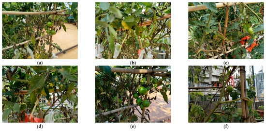
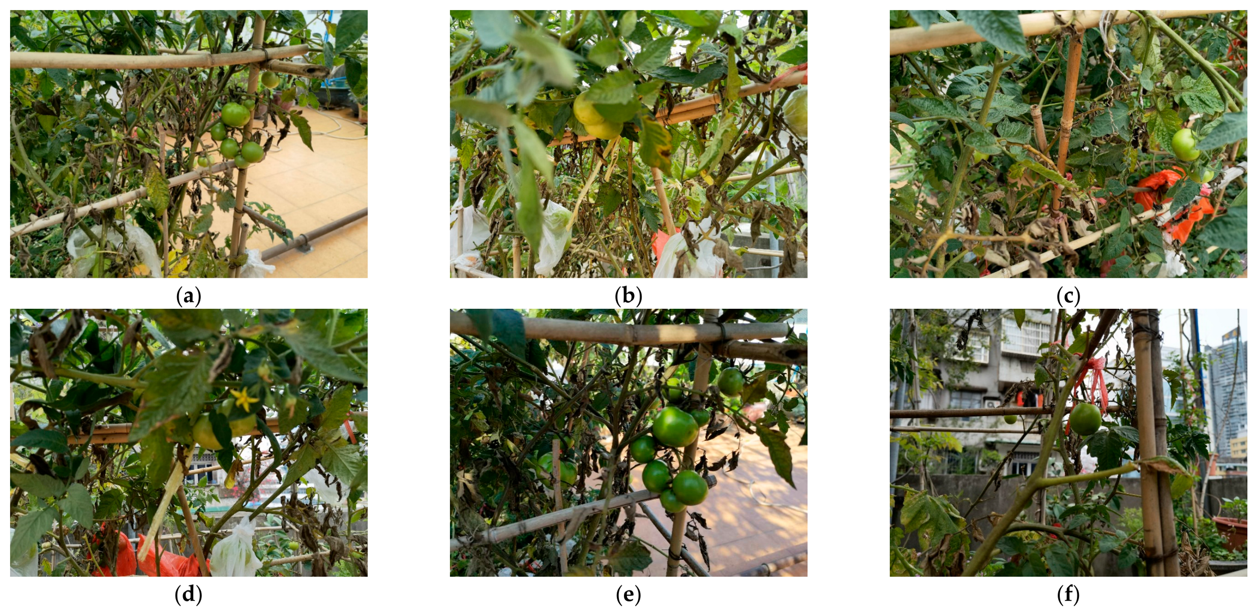
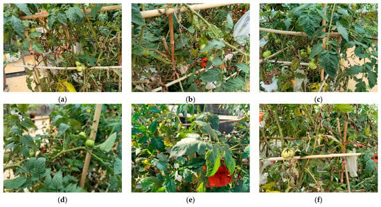
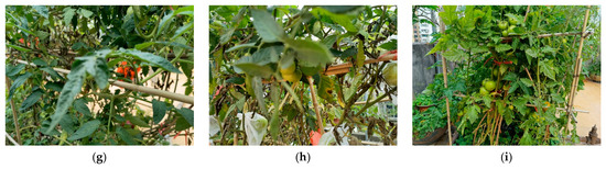
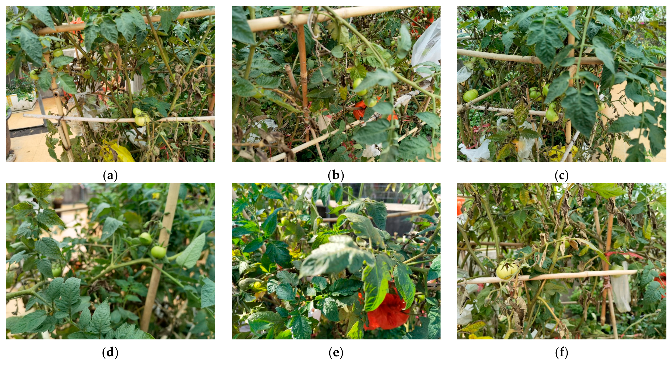
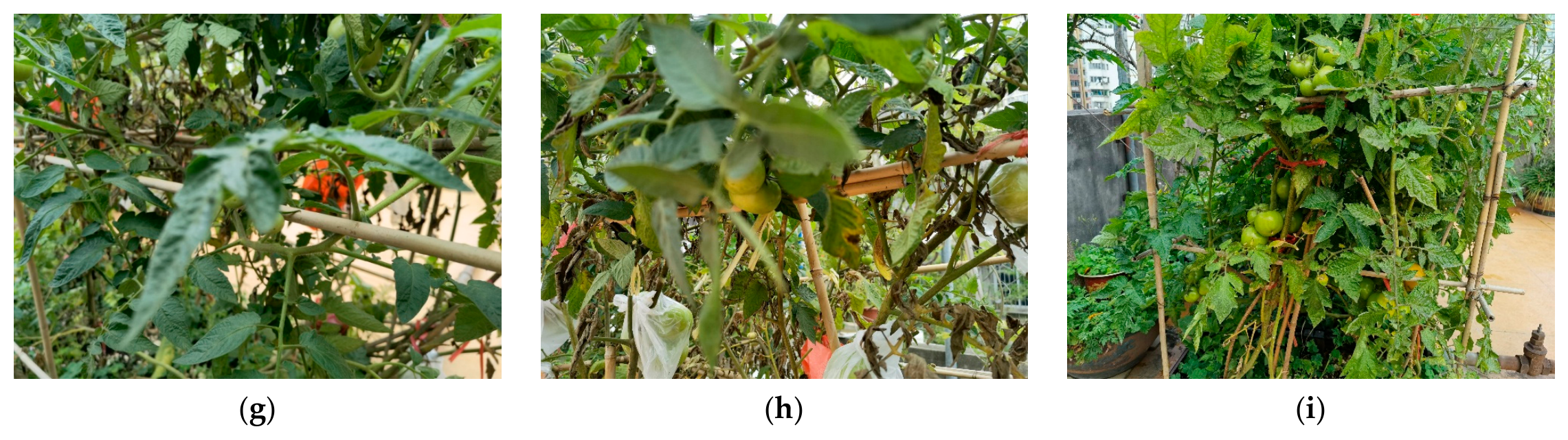
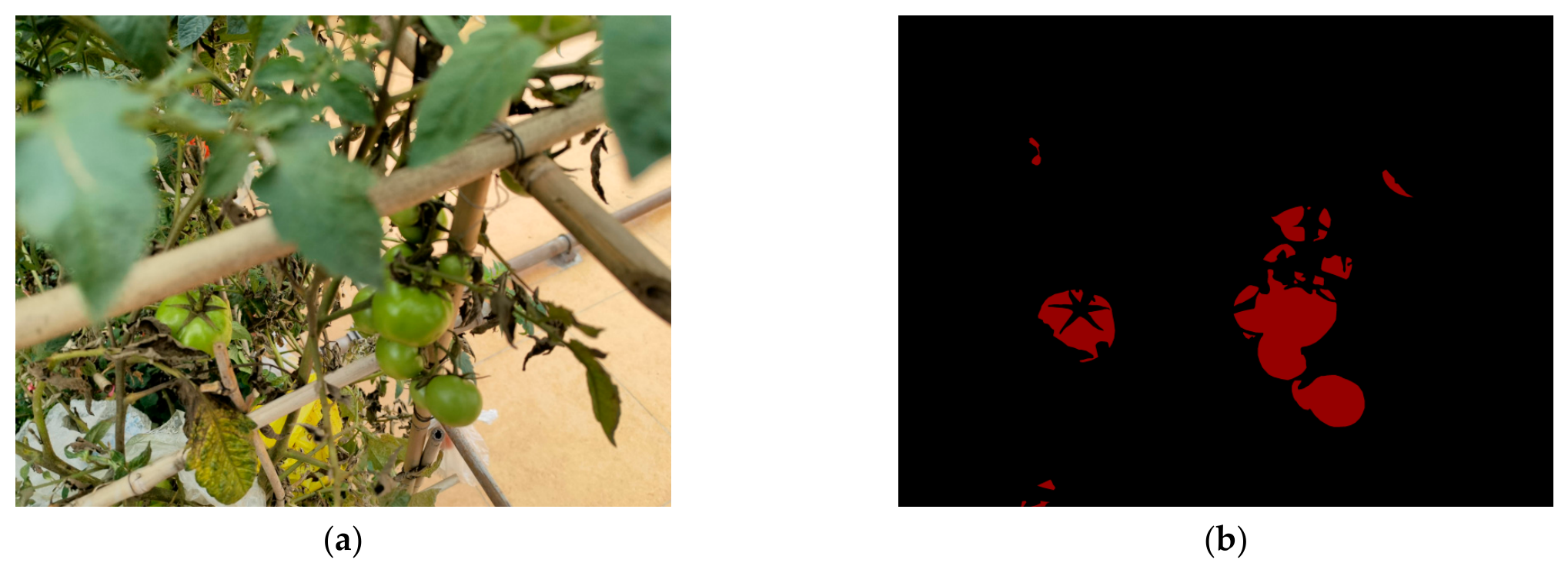
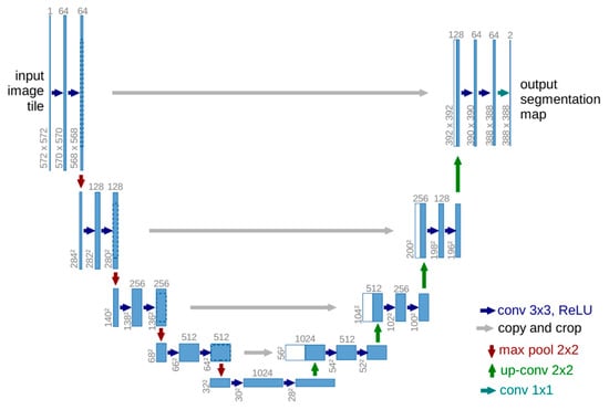
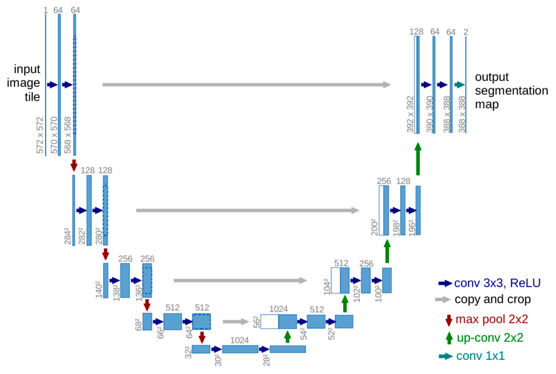
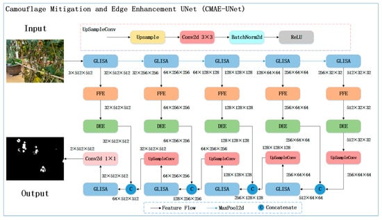
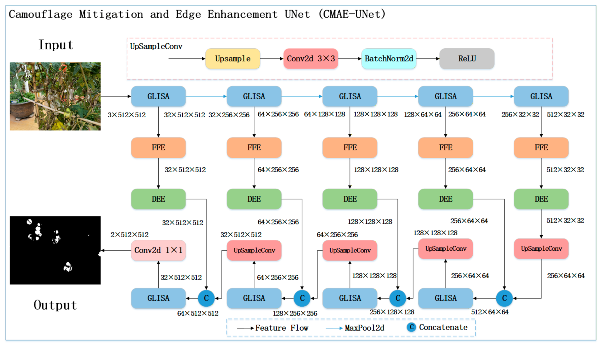
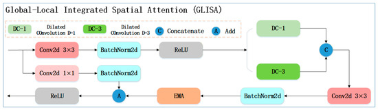
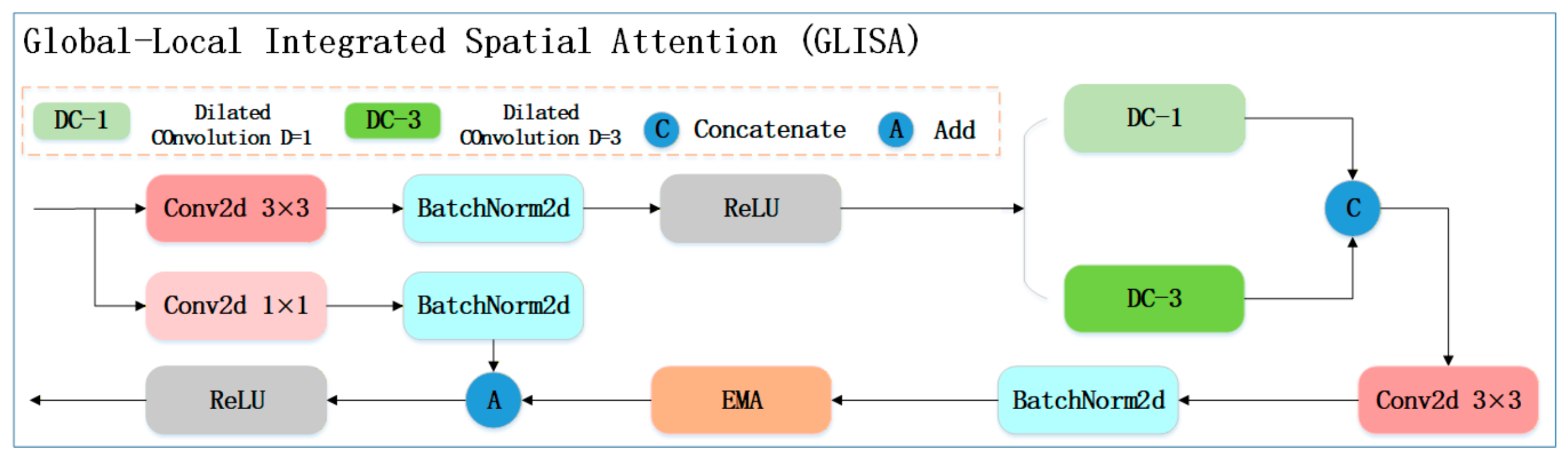
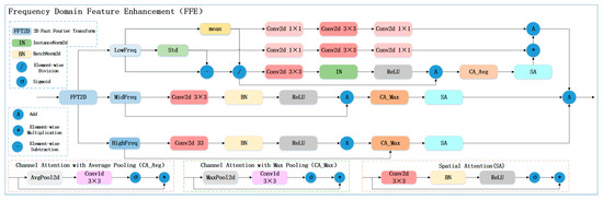
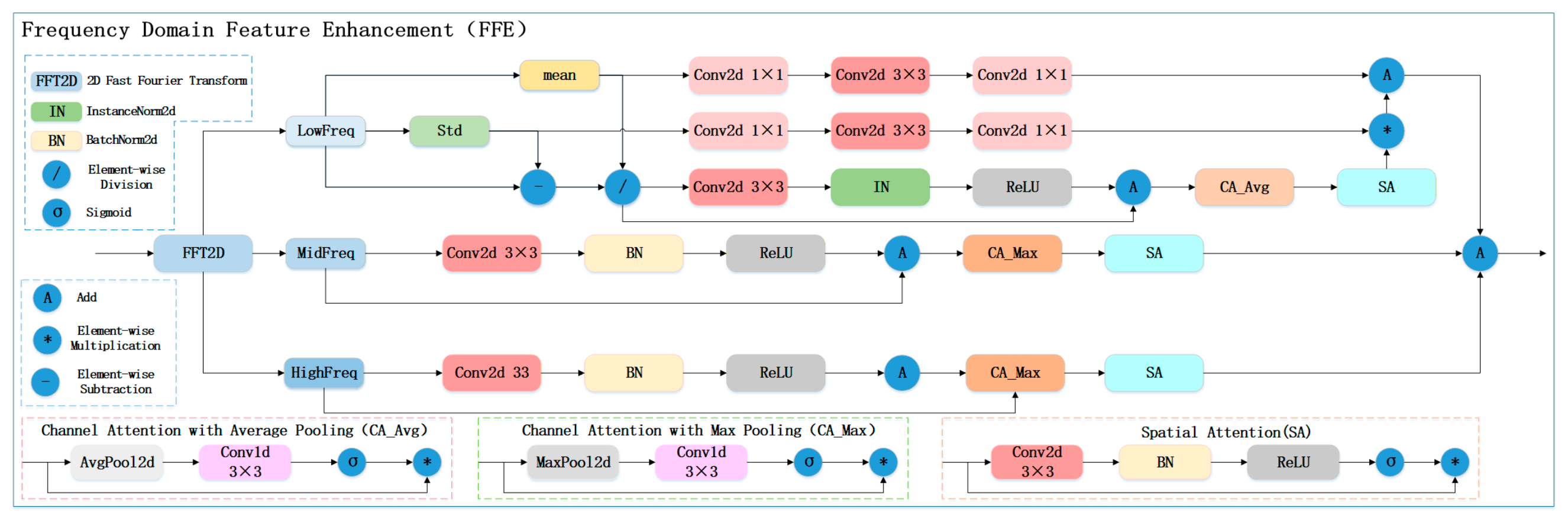
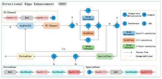
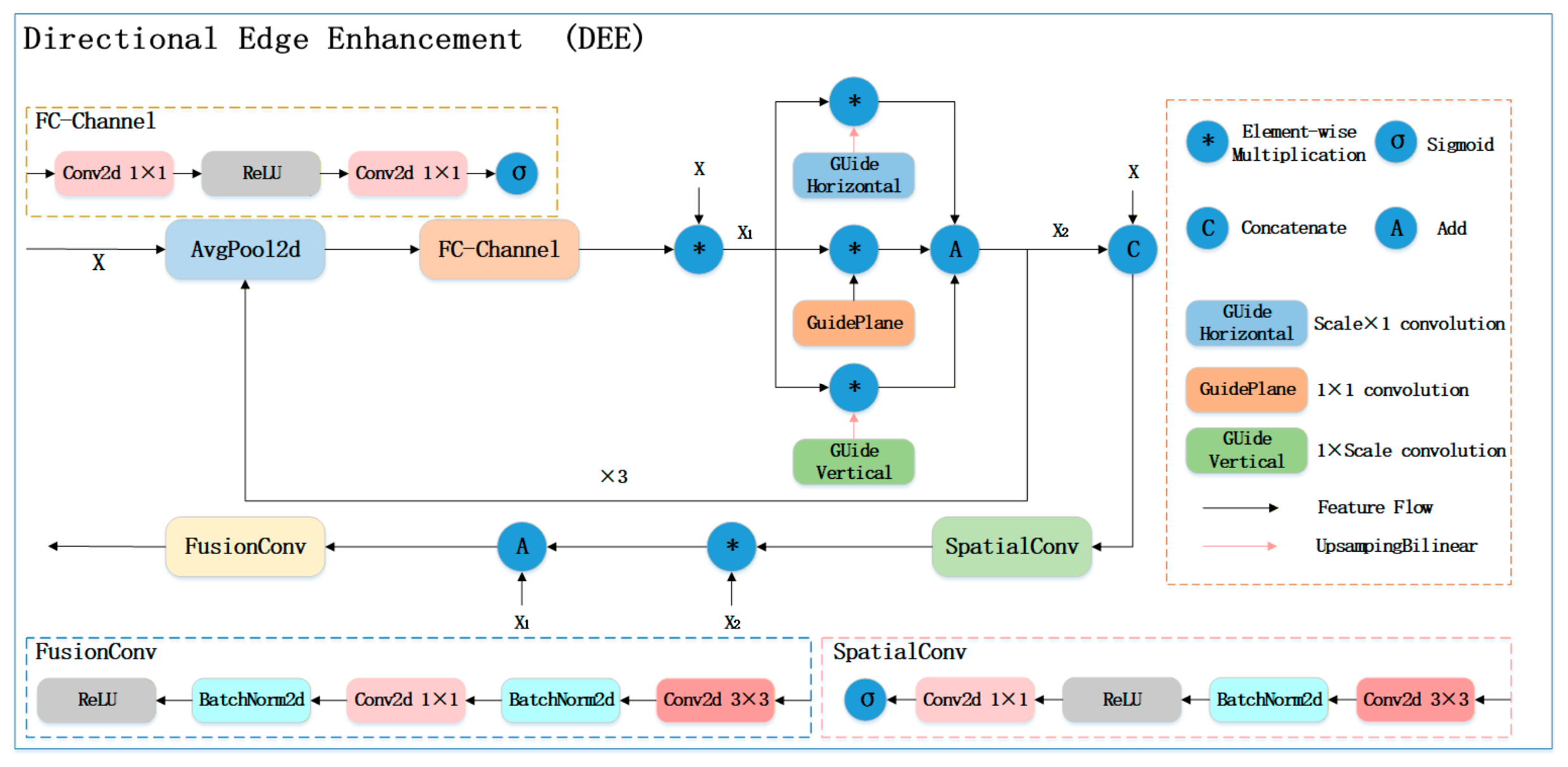
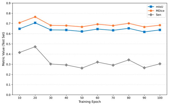
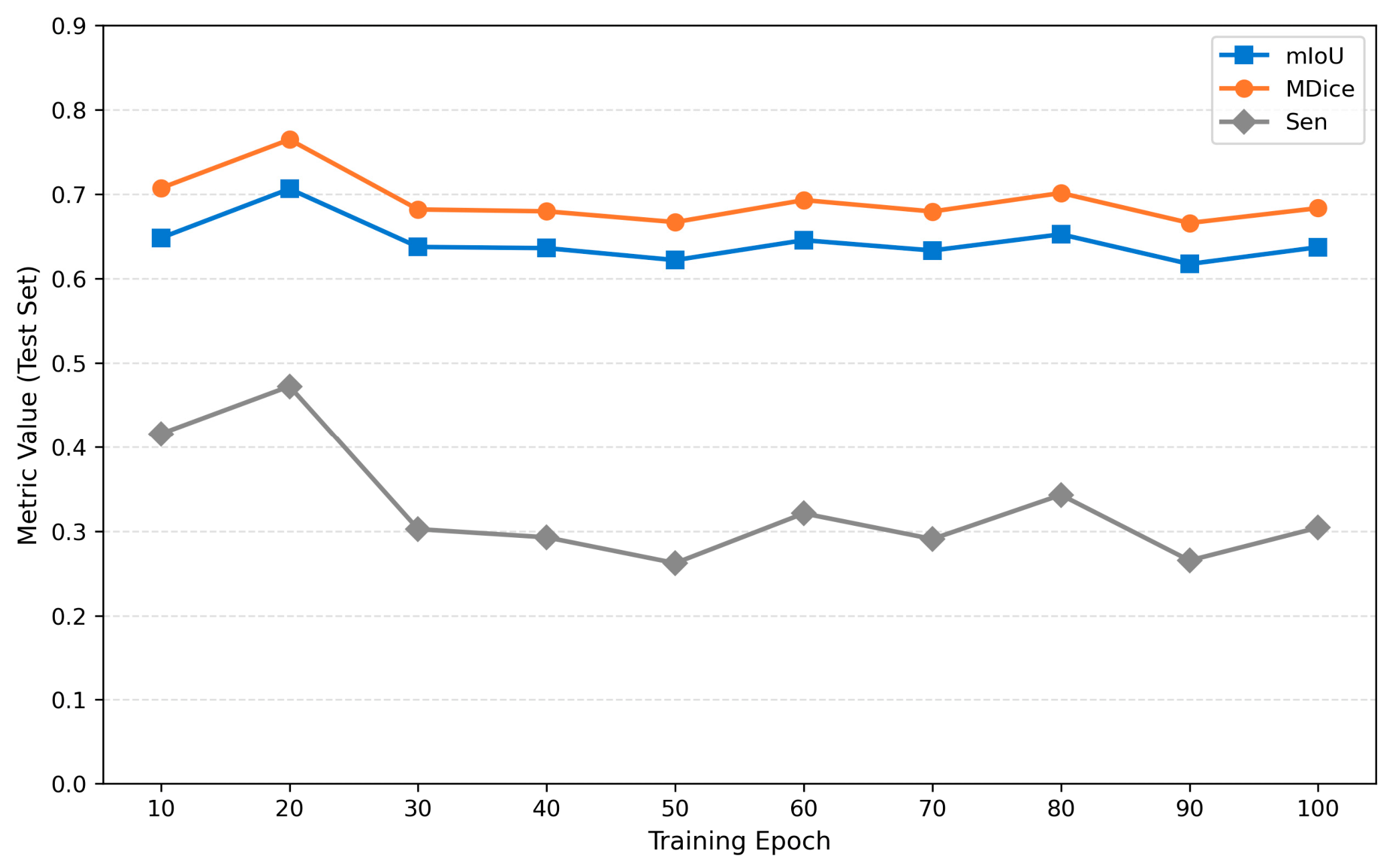
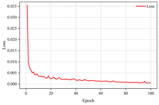
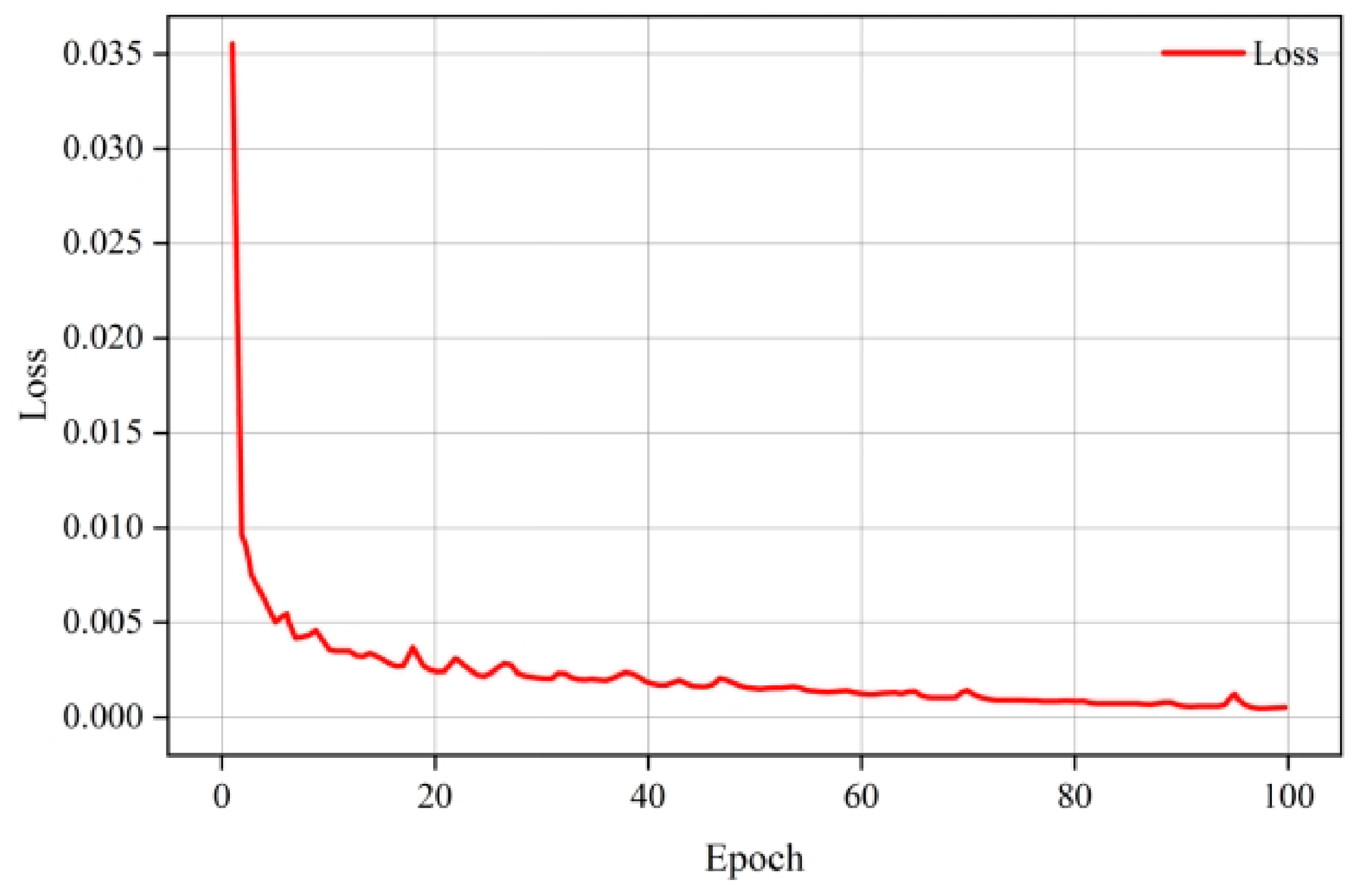
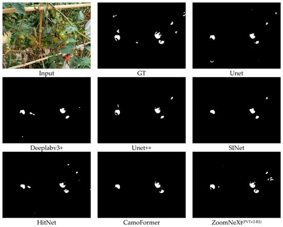
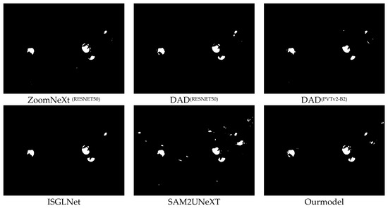
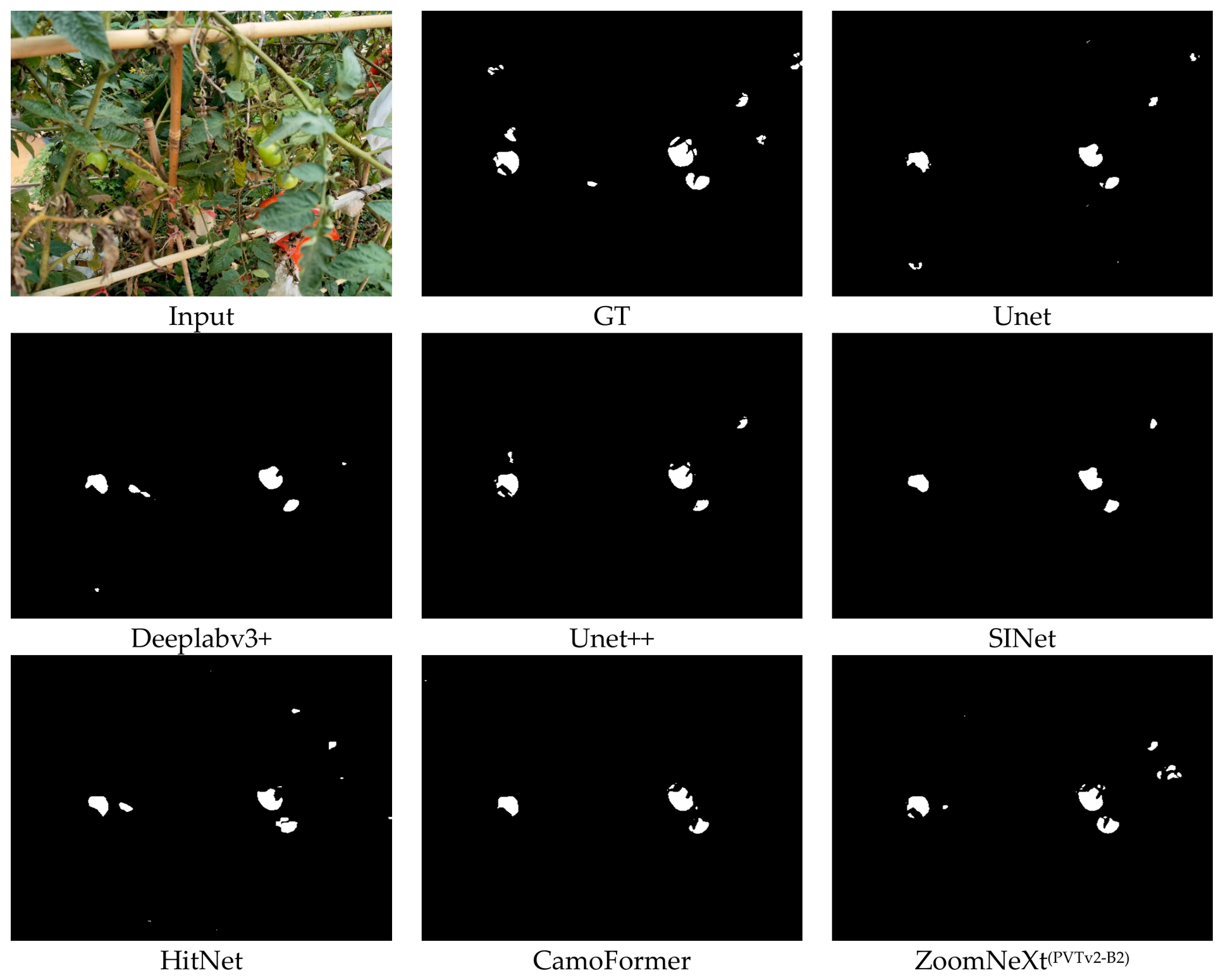
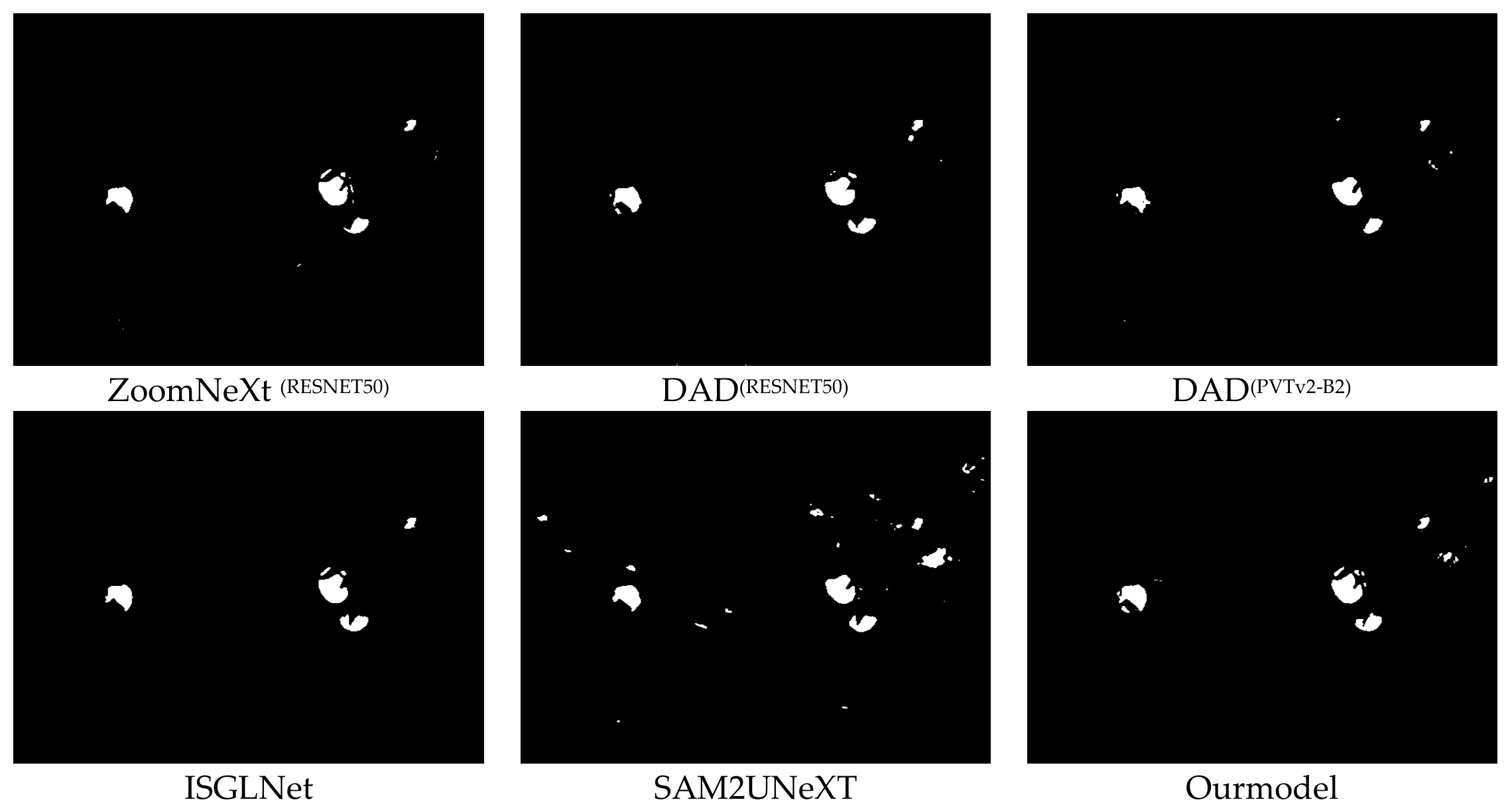
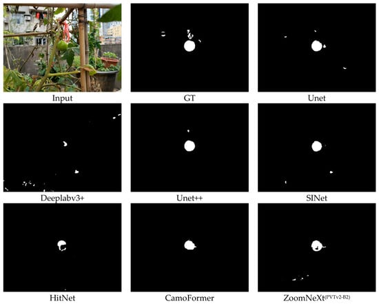
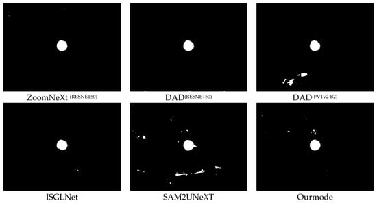
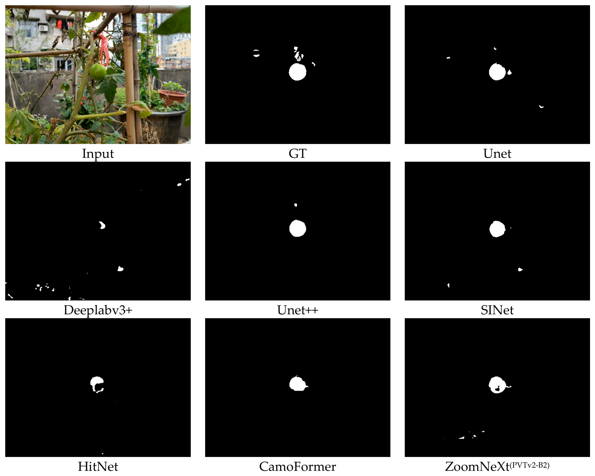
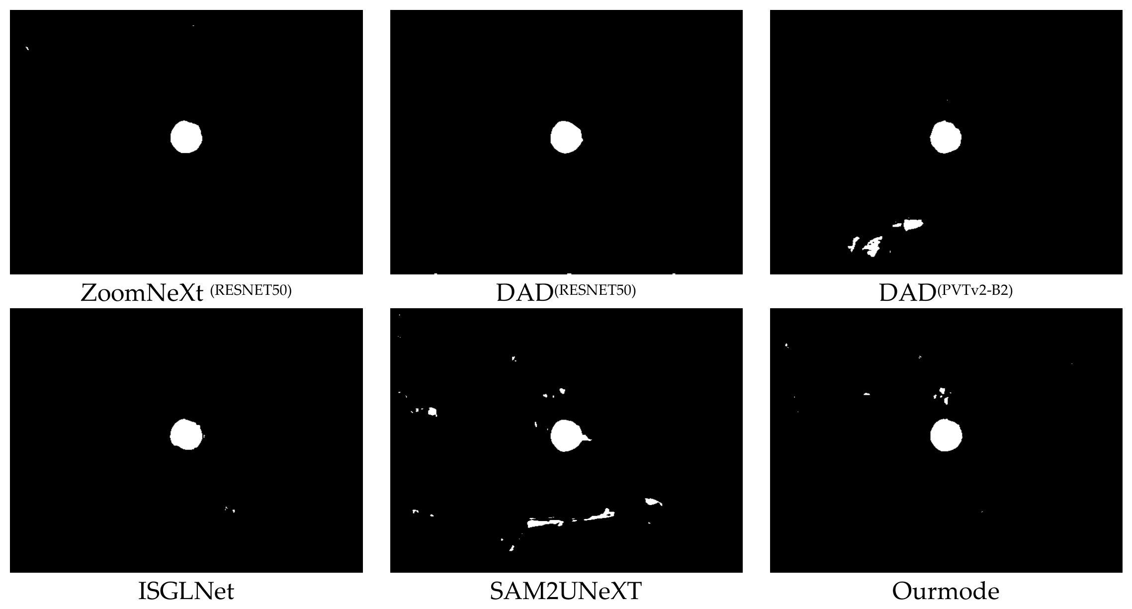
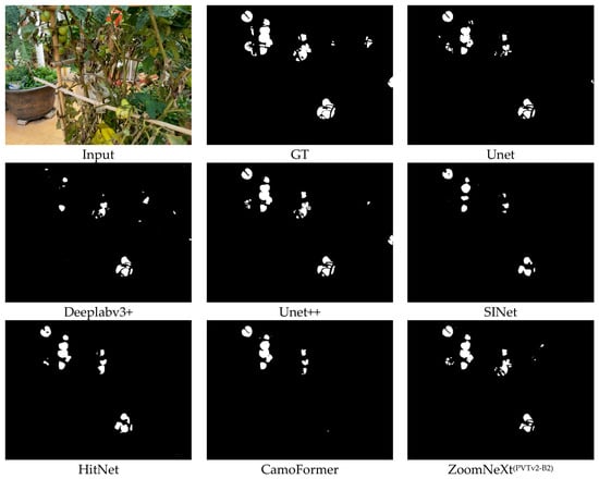
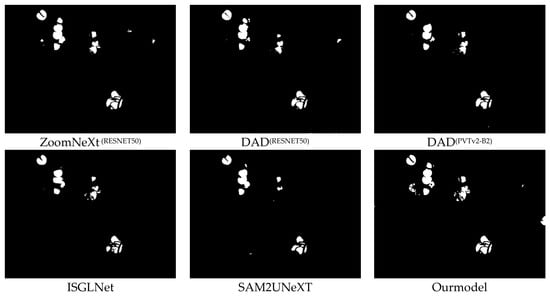
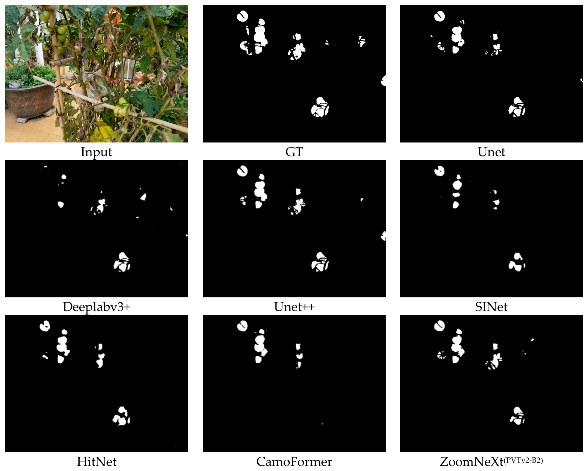
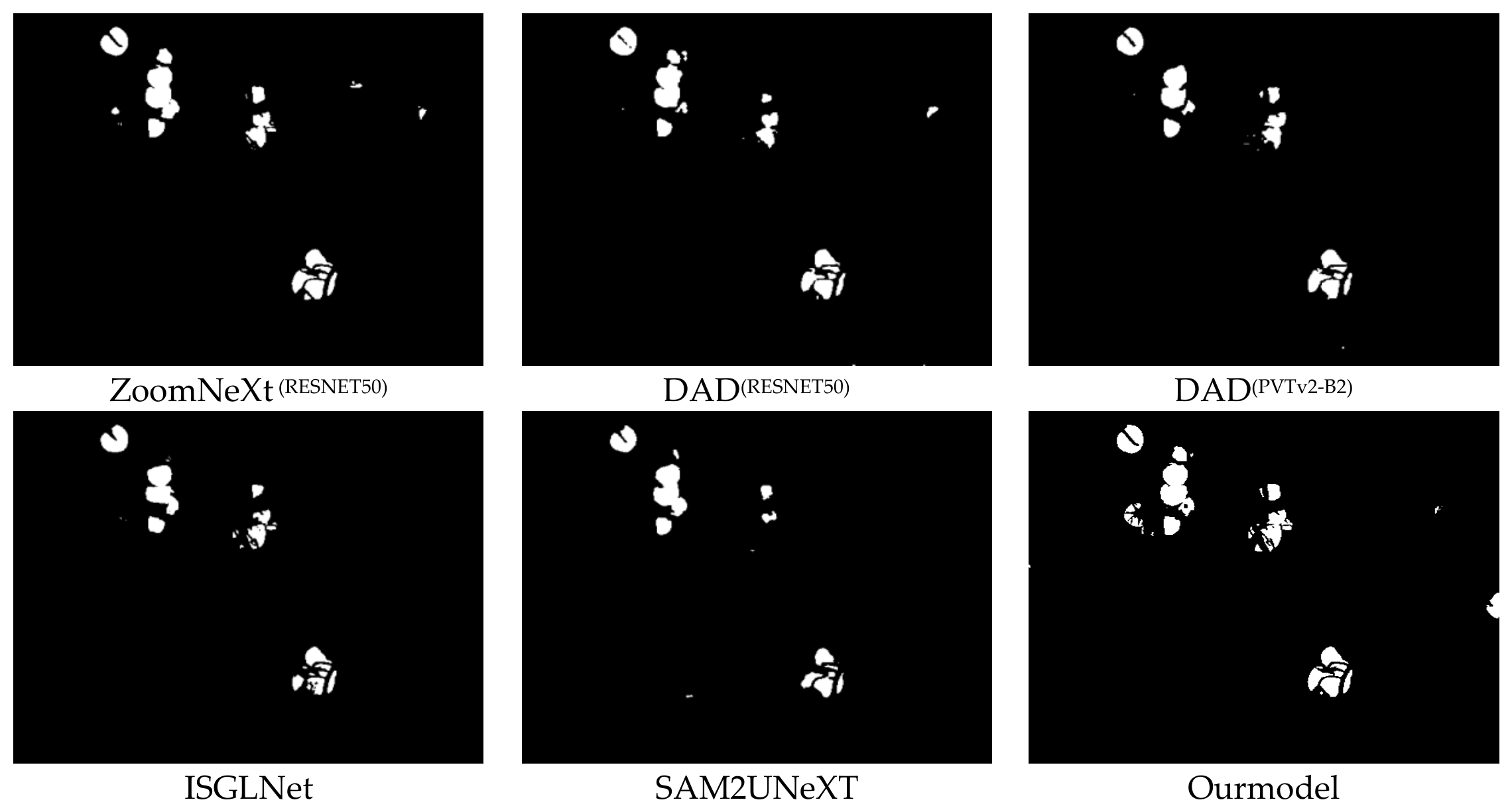
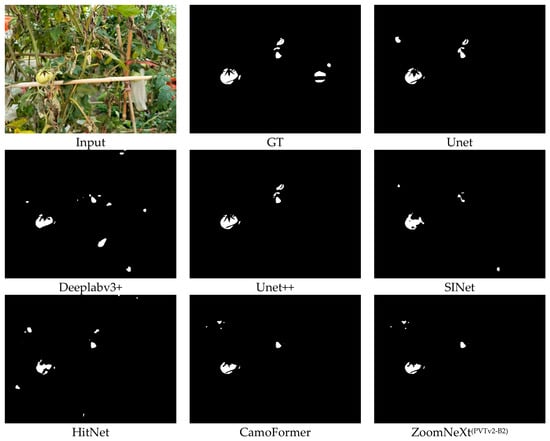
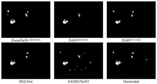
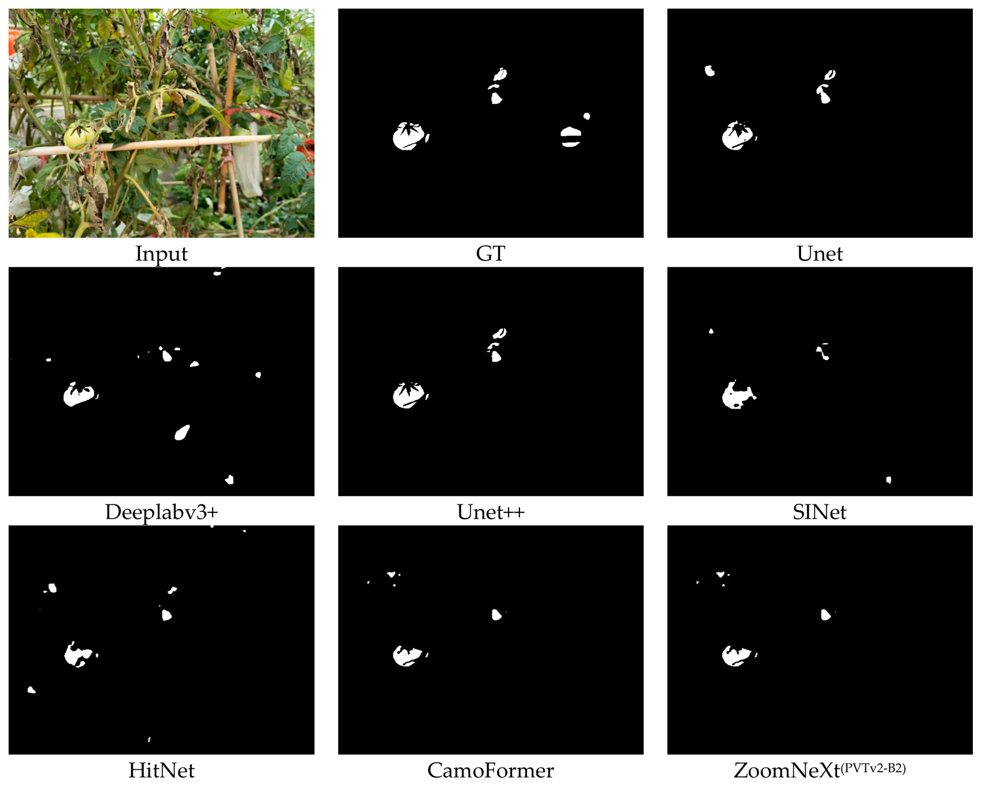
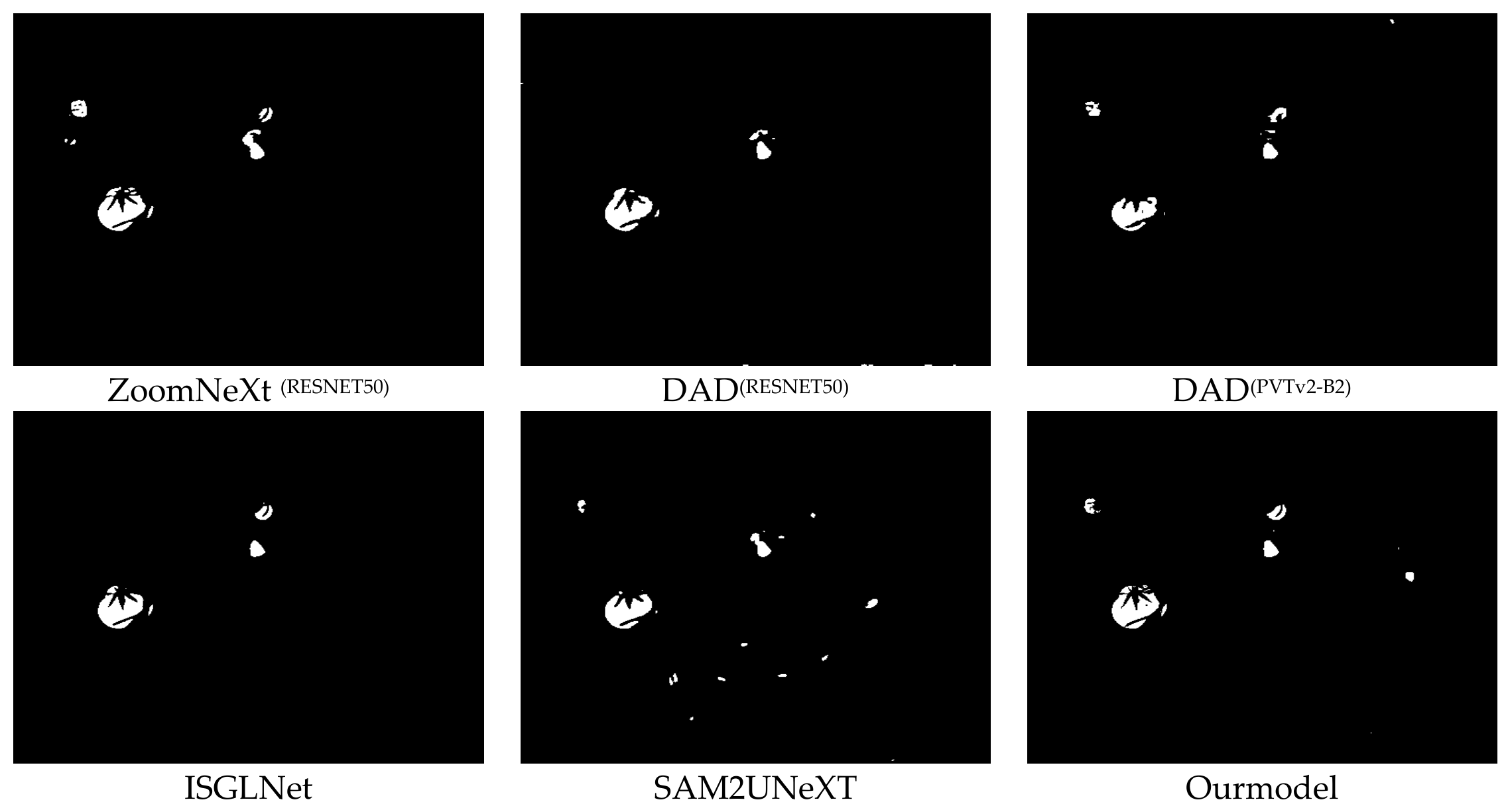
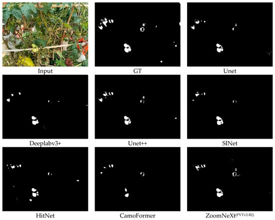
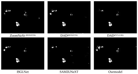
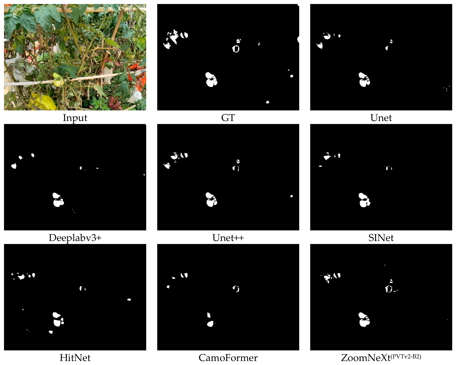
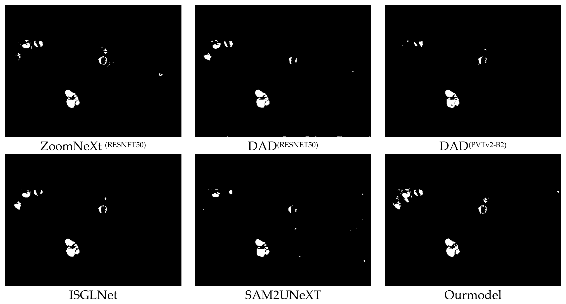
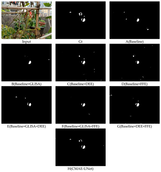
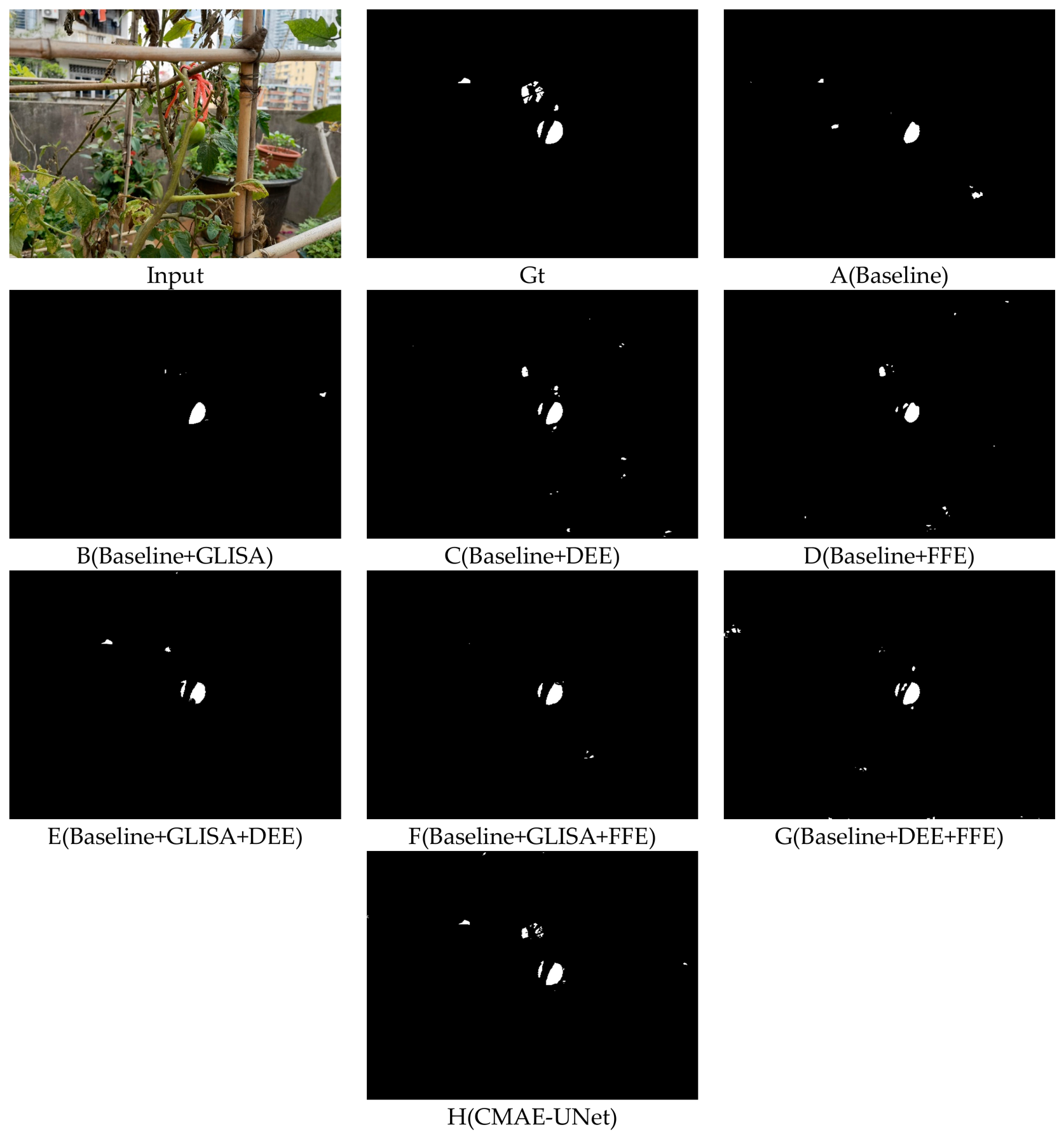

Disclaimer/Publisher’s Note: The statements, opinions and data contained in all publications are solely those of the individual author(s) and contributor(s) and not of MDPI and/or the editor(s). MDPI and/or the editor(s) disclaim responsibility for any injury to people or property resulting from any ideas, methods, instructions or products referred to in the content. |
© 2026 by the authors. Licensee MDPI, Basel, Switzerland. This article is an open access article distributed under the terms and conditions of the Creative Commons Attribution (CC BY) license.