


Abstract
Soil spatial variability is a key driver of tree development in perennial crops, and its characterisation is essential for precision orchard management. Against this background, soil–canopy relationships were investigated in a Citrus reticulata Blanco cv. Tango orchard under Mediterranean conditions. Electromagnetic induction (EMI), unmanned aerial vehicle (UAV) multispectral imagery, and mobile LiDAR data registered using a Simultaneous Localisation and Mapping (SLAM) workflow were integrated at individual-tree level. A previously validated EMI-derived apparent electrical conductivity (ECa) layer was used as a baseline descriptor of soil variability. UAV and mobile LiDAR acquisitions were harmonised for 40 trees: LiDAR point clouds were voxelised to derive canopy structural traits, while UAV imagery provided Soil-Adjusted Vegetation Index (SAVI) values. ECa at 14 kHz was negatively correlated with canopy volume (r = −0.605, R2 = 0.365) and canopy volume-to-projected area ratio (r = −0.571, R2 = 0.326), both significant at p < 0.001. Conversely, SAVI showed a weaker, non-significant relationship with ECa (r = −0.285, R2 = 0.081, p = 0.0749). The reduced multiple linear regression model explained canopy volume variability (R2 = 0.804), retaining canopy diameter and ECa as significant predictors. These findings highlight the value of LiDAR-derived structural traits as sensitive indicators of soil-related canopy variability, supporting the integration of structural, spectral, and soil-sensing data for site-specific orchard management.
1. Introduction
Spatial heterogeneity is a defining feature of agricultural soils and one of the main reasons why trees growing within the same orchard often differ in size, vigour, and productivity [1,2].
In perennial systems, soil-related constraints may persist over time and interact with irrigation, root development, and canopy growth, generating stable within-orchard patterns that are difficult to detect through conventional field observations alone [1,3]. This is particularly relevant in Mediterranean environments, where limited water availability and heterogeneous soil conditions frequently coexist and may amplify tree-to-tree variability [2,4]. For this reason, site-specific approaches are increasingly important for improving orchard management and interpreting how local soil conditions shape plant performance. Among proximal sensing techniques, electromagnetic induction (EMI) is widely used to characterise soil variability rapidly and non-destructively through apparent soil electrical conductivity (ECa) [1]. ECa is an integrative proxy rather than a single soil attribute, as it reflects the combined influence of texture, coarse fragments, organic carbon, water content, salinity, temperature, and bulk density [1,5]. This makes EMI useful for field-scale soil characterisation and management-zone delineation, although ECa patterns must be interpreted within their agronomic and environmental context. In orchard systems, especially under micro-irrigation, ECa may capture both texture-related differences and spatial effects associated with localised wetting patterns and plant water uptake [3,5]. Recent evidence from citrus orchards has further highlighted the relationship between ECa and particle-size fractions, reinforcing the value of EMI-based sensing for soil characterisation in tree crops [4]. Beyond its use for mapping physical soil variability, EMI-derived ECa has also been related to soil organic carbon, soil CO2 emissions, soil microbiological indicators, and product-quality attributes in Mediterranean perennial systems [6,7,8,9]. This broader agronomic relevance supports the use of EMI not only as a soil-mapping tool, but also as a screening layer for interpreting spatial patterns in soil–plant interactions. In citrus orchards, this interpretation is particularly relevant because finer-textured or more conductive soil conditions may influence water retention, drainage, and root-zone aeration, with potential consequences for cumulative canopy development. Therefore, linking ECa patterns with canopy traits can help identify spatial gradients that are not immediately evident from visual field observations alone. While soil mapping provides the pedological background, orchard tree response must also be described at canopy level.
Canopy architecture is closely linked to light interception, transpiration, biomass accumulation, and orchard management efficiency, and therefore represents a key target in precision horticulture [10,11]. In recent years, LiDAR-based sensing and point-cloud analysis have enabled the quantification of structural traits such as canopy height, canopy diameter, volume, projected area, and trunk-related parameters with a level of spatial detail that was previously difficult to achieve under field conditions [10,11,12,13]. Recent studies on citrus orchards have addressed canopy volume extraction from three-dimensional point clouds using approaches such as voxel-based, convex-hull, alpha-shape, and slicing-based methods [14,15].
In orchards, LiDAR-derived traits have supported tree-scale characterisation and crop monitoring [11,12]. Recent reviews have highlighted the role of LiDAR platforms in precision agriculture, particularly for crop structure assessment, canopy monitoring, and three-dimensional trait extraction [16,17]. At the same time, more accessible solutions based on smartphone photogrammetry and embedded LiDAR sensors have shown promising performance, suggesting that three-dimensional canopy assessment may also be feasible in operational agricultural settings [18,19]. Compared with static terrestrial laser scanning, SLAM-based mobile LiDAR can improve acquisition efficiency by allowing continuous scanning along orchard rows and reducing the need for multiple fixed scan positions [16,17,18]. In addition, SLAM-based acquisition can provide relative three-dimensional reconstruction without requiring a dense ground-control setup and is particularly suitable for structurally complex orchard environments, where occlusions and narrow inter-row spaces may limit static scanning configurations.
UAV multispectral imagery provides canopy spectral information by capturing canopy reflectance and enabling the derivation of vigour-related indices at high spatial resolution [10,20]. Recent reviews have shown that UAV-based sensing is increasingly used in orchard monitoring for canopy assessment, tree detection, vigour mapping, and management support [21,22].
In heterogeneous orchard systems, this type of information has proved useful for tree crown delineation, canopy monitoring, and vigour mapping, including in citrus-based environments [20]. UAV multispectral and photogrammetric data have also been used to extract structural properties of tree crops and to assess pruning effects [23]. Previous UAV-based studies have further shown that multispectral imagery and photogrammetric surface models can support individual citrus tree extraction and canopy delineation [24,25]. However, spectral data alone do not fully describe the three-dimensional organisation of the canopy. Conversely, structural measurements derived from point clouds may capture canopy size and spatial occupation without directly describing spectral or physiological status. In citrus orchards, UAV-derived canopy shape descriptors and vegetation indices have been shown to provide complementary information on tree condition, further supporting the need to interpret spectral and structural variables together [26]. For this reason, the joint interpretation of structural and spectral information can provide a more informative framework for assessing plant variability, particularly where tree performance is influenced by heterogeneous soil conditions [10,13].
Despite the growing availability of these sensing approaches, studies explicitly combining soil mapping, canopy structural analysis, and canopy spectral assessment within the same orchard framework remain relatively limited, particularly in citrus systems, where UAV-based monitoring and LiDAR-based canopy reconstruction have often been addressed separately. Most available studies focus on one component at a time, addressing either soil variability, canopy structure, or remotely sensed vigour separately [3,4,10,18]. In a previous study, an integrated workflow based on EMI, Sentinel-2 data, and laboratory analyses proved effective for describing Mediterranean topsoil variability and delineating soil management zones [27]. Building on that pedological basis, the present study extends the analysis to the plant component by integrating mobile-LiDAR-derived canopy traits with UAV-derived spectral indicators at tree level.
The aim of this study was therefore to investigate the relationships between soil variability, canopy structure, and canopy spectral response in a commercial Citrus reticulata Blanco cv. Tango orchard using an integrated multi-sensor approach. Multi-frequency EMI was used to describe soil spatial patterns, SLAM-registered mobile LiDAR point clouds were processed to extract structural canopy traits, and UAV multispectral imagery was used to derive canopy spectral indicators. We hypothesised that tree-level ECa would be associated with measurable differences in canopy volume and structural traits and, to a lesser extent, with canopy spectral response as described by SAVI. By integrating soil, structural, and spectral information within a harmonised tree-level framework, this study aimed to provide a high-resolution interpretation of soil–plant interactions in support of site-specific orchard management.
2. Materials and Methods
2.1. Study Area and Climatic Context
The study was conducted in the Sele Plain, a coastal alluvial basin in Campania, southern Italy, recognised as one of the main Mediterranean agricultural districts (Figure 1a). The experimental orchard is located in the municipality of Eboli, Salerno province (40°35′08″ N, 15°03′54″ E), at an average elevation of 54 m a.s.l., and covers approximately 2.5 ha.
Figure 1.
(a) Location of the experimental site in southern Italy (Sele Plain, Campania); the Campania Region is outlined in light green and Italian regions are shown in white for clarity. (b) Boundary of the experimental field, delineated in yellow, with north arrow and scale bar for spatial reference. (c) Ground-level view of the experimental orchard planted with Citrus reticulata Blanco cv. Tango.
The boundary of the field is shown in Figure 1b, while a ground-level view of the orchard planted with Citrus reticulata Blanco cv. Tango is reported in Figure 1c. At the time of the UAV and mobile LiDAR acquisitions in 2024, the trees were four years old.
The area is intensively cultivated and characterised by pronounced soil heterogeneity, likely associated with alluvial dynamics, long-term agricultural use, and irrigation management, as previously documented for the same experimental field through EMI mapping, satellite-derived soil indicators, and laboratory analyses [27]. The orchard was managed according to standard commercial practices for citrus production in the area, including regular irrigation, fertilisation, and canopy management. Water distribution uniformity within the irrigation system had been previously assessed in the experimental field, and no relevant differences were detected between the northern and southern sectors. This assessment supported the interpretation that the observed spatial differences in canopy development were not primarily attributable to irrigation non-uniformity. Mechanical topping was performed in February 2024 to control tree height and maintain a relatively uniform canopy architecture along the rows. This operation was considered relevant for interpreting UAV-derived spectral patterns, as it may have contributed to reducing between-tree variability in canopy shape and external canopy expression during the subsequent growing season.
To provide environmental context for the survey year, daily climatic data recorded in 2024 were obtained from the Eboli-Improsta agrometeorological station, managed by the Campania Region Agrometeorological Service [28] (Figure 2). Daily records were aggregated at monthly scale: minimum, mean, and maximum air temperatures were expressed as monthly averages of daily values, whereas precipitation was expressed as cumulative monthly rainfall. In 2024, the mean annual air temperature was 17.6 °C, with annual averages of daily minimum and maximum temperatures of 12.7 °C and 23.2 °C, respectively. Total annual precipitation was 538.8 mm.
Figure 2.
Monthly climatic conditions recorded in 2024 at the Eboli-Improsta agrometeorological station. Minimum, mean, and maximum air temperatures are shown in the upper panel, while cumulative precipitation is shown in the lower panel. The shaded area indicates October, when UAV multispectral and mobile LiDAR acquisitions were carried out.
The climatic pattern was characterised by mild winter temperatures, a progressive increase from spring to summer, and a dry summer period. Rainfall was mainly concentrated in winter and early autumn, whereas precipitation was very limited during late spring and summer, with 2.4 mm in June and 0.0 mm in July. The mobile LiDAR and UAV acquisitions were carried out in October 2024, when mean air temperature was 19.1 °C and cumulative monthly precipitation was 57.6 mm, providing the climatic context for interpreting canopy structural and spectral conditions at the time of survey.
2.2. Overall Experimental Workflow and Data Integration
The study integrated three complementary sources of information describing soil conditions, canopy structure, and canopy spectral response within the same commercial Citrus reticulata Blanco cv. Tango orchard. The analytical framework combined: (i) a baseline soil dataset derived from a previously published electromagnetic induction (EMI) survey of the experimental field [27]; (ii) newly acquired SLAM-registered mobile LiDAR point clouds used to quantify structural canopy traits; and (iii) UAV multispectral imagery acquired to derive canopy spectral indicators.
The individual tree was used as the final analytical unit, allowing soil, structural, and spectral variables to be compared within a common spatial framework. The soil component was represented by EMI-derived apparent electrical conductivity (ECa), used as a proxy for within-field soil physical variability. The structural component was obtained from voxel-based processing of SLAM-registered mobile LiDAR point clouds and included canopy volume, canopy height, horizontal canopy diameter, basal stem diameter, and the canopy volume-to-projected area ratio, used as a structural descriptor of canopy occupation. The spectral component was based on tree-level values extracted from processed multispectral orthomosaics, with the Soil-Adjusted Vegetation Index (SAVI) selected as the main tree-level canopy spectral descriptor. After sensor-specific preprocessing, all variables were spatially aligned at individual-tree scale to generate a single dataset for statistical analysis.
This workflow enabled soil–plant relationships to be evaluated by combining baseline pedological variability with canopy architecture and spectral behaviour under field conditions, as illustrated in Figure 3.
Figure 3.
Conceptual workflow of the integrated multi-sensor approach used to analyse soil–canopy relationships at individual-tree level. EMI, UAV multispectral imagery, and mobile LiDAR data processed through a SLAM-based workflow were used to derive tree-level soil, spectral, and structural variables, which were then harmonised into a common dataset for integrated statistical analysis.
2.3. Baseline Soil Dataset and EMI-Derived Conductivity Layer
The soil component used in this study was derived from a previously published electromagnetic induction survey conducted on the same experimental field prior to orchard establishment [27]. The survey was performed under bare-soil and dry conditions, reducing vegetation-related interference and limiting the influence of transient surface moisture on the apparent electrical conductivity signal. Detailed information on survey design, acquisition conditions, and laboratory validation of soil properties is reported in Lepore et al. [27].
In the present study, the pre-planting EMI-derived ECa layer was used as a baseline pedological descriptor of the experimental field. This interpretation was supported by the previous validation carried out on the same site, where the 14 kHz ECa spatial pattern was assessed under bare-soil and dry survey conditions and related to Sentinel-1 moisture information, laboratory-measured soil properties, and Sentinel-2-derived Clay Index values [27]. The relationship between ECa and the Sentinel-1 moisture proxy was weak and non-significant, whereas ECa showed strong positive associations with clay-related indicators, including laboratory-measured clay content and the Sentinel-2-derived Clay Index [27].
Therefore, the conductivity gradient used here was interpreted as representative of a relatively stable texture-related soil background, rather than as a transient soil-moisture pattern, and was considered suitable for investigating cumulative differences in canopy structural development. This use was based on the assumption that the main texture-related spatial pattern, particularly clay-related variability, is comparatively stable over time relative to short-term soil moisture fluctuations and seasonal canopy spectral responses.
The EMI survey was carried out using a GSSI Profiler EMP-400 (Geophysical Survey Systems Inc., Nashua, NH, USA), operated in vertical dipole mode at three frequencies (14, 7, and 3 kHz), selected to characterise progressively deeper apparent soil responses, with the higher frequency providing greater sensitivity to shallower soil variability and the lower frequencies integrating deeper soil volumes.
The instrument was held approximately 20 cm above the ground while walking along parallel transects covering the entire field. Data were acquired at 4–5 km h−1 with a logging interval of 0.75 s, resulting in 3158 georeferenced measurements across approximately 2.5 ha. Raw data were initially processed in MagMap2000 (version 4.86, Geophysical Survey Systems Inc., Nashua, NH, USA), where spurious readings were removed before export for spatial analysis. After duplicate filtering, retaining the first record at coincident coordinates, EMI point data were used to generate an interpolated ECa raster in QGIS using the Smart-Map tool.
The 14 kHz ECa raster was produced at a spatial resolution of 0.20 m and used as the analytical soil conductivity layer for tree-level extraction. Among the three frequencies, the 14 kHz ECa layer was retained as the main soil predictor because it had previously been identified as the most representative of shallow soil variability at the study site [27]. For graphical representation of the field-scale conductivity pattern, the EMI data were also visualised in Surfer 23 (Golden Software, LLC, Golden, CO, USA).
2.4. UAV Multispectral Acquisition and SAVI Extraction
UAV multispectral monitoring was performed to characterise canopy spectral response and provide a spectral layer suitable for integration with soil and structural data. Multispectral imagery was acquired over the experimental orchard using a DJI Phantom 4 Multispectral platform, equipped with one RGB sensor for visible-light imaging and five monochrome sensors for multispectral acquisition. The spectral bands of the multispectral sensor are reported in Table 1.
Table 1.
Spectral bands of the DJI Phantom 4 Multispectral sensor used for UAV-based canopy spectral assessment.
The UAV acquisition used in the present analysis was carried out on the same date and within the same morning time window as the mobile LiDAR survey, in order to ensure temporal consistency between spectral and structural observations. The flight was performed under stable illumination conditions following a nadir grid mission at 50 m above ground level, with 80% front and side overlap and a flight speed of 5 m s−1. A total of 1001 images were acquired, resulting in a ground sampling distance of approximately 0.027 m pixel−1 in width and 0.025 m pixel−1 in height.
Photogrammetric processing was performed in Agisoft Metashape Professional (version 1.8.2, Agisoft LLC, St. Petersburg, Russia), including image alignment, dense point-cloud generation, digital surface model reconstruction, and multispectral orthomosaic generation. Among the computed vegetation indices, the Soil-Adjusted Vegetation Index was retained as the main spectral descriptor because of its reduced sensitivity to exposed soil background, which is particularly relevant in young orchard systems where inter-row soil exposure and discontinuous canopy cover may influence spectral responses [20,29]. SAVI was calculated as follows [29]:
where and are the radiometrically processed near-infrared and red band values used for index calculation, respectively.
In accordance with the original SAVI formulation [29], was set to 1 to reduce the potential influence of exposed soil and mixed pixels associated with the young and discontinuous canopy structure of the orchard.
Tree-level SAVI values were extracted by applying canopy polygons as zonal masks, so that only canopy pixels contributed to the mean value assigned to each tree. Canopy polygons were delineated from the digital surface model by separating elevated canopy objects from the surrounding ground and inter-row surface. The resulting polygons were visually inspected and manually corrected, when necessary, by the same operator to exclude inter-row soil, residual ground pixels, and mixed pixels along canopy margins, while preserving the visible crown footprint of each analysed tree.
The same canopy polygons were also used to derive the MSI-based canopy area included in the integrated tree-level dataset. The resulting canopy-specific SAVI values were then integrated with mobile-LiDAR-derived structural traits and EMI-derived ECa.
2.5. Mobile LiDAR Acquisition, SLAM-Based Registration, Point-Cloud Processing and Voxel-Based Trait Extraction
2.5.1. Mobile LiDAR and SLAM-Based Point-Cloud Processing
Three-dimensional structural surveys were conducted using a GeoSLAM ZEB Horizon RT mobile laser scanner (FARO Technologies Inc., Lake Mary, FL, USA) to quantify tree architecture at individual-tree scale. LiDAR-based approaches have been increasingly applied in orchard and tree-crop systems for three-dimensional canopy reconstruction and the estimation of structural plant traits [30,31,32].
Raw scan data were processed using FARO Connect, formerly GeoSLAM Connect, to perform Simultaneous Localisation and Mapping (SLAM)-based registration and generate the registered three-dimensional mobile LiDAR point cloud.
Scanning was performed by moving along the orchard rows according to the manufacturer’s operational guidelines, while maintaining a regular trajectory around the trees to maximise canopy coverage and reduce occluded sectors within the reconstructed cloud. The mobile LiDAR survey was focused on the selected orchard rows representing the contrasting ECa conditions identified from the baseline EMI map. To speed up transfers between adjacent rows and facilitate field operations, the operator carrying the instrument was assisted by a support vehicle during the survey.
2.5.2. Point-Cloud Preprocessing and Tree Segmentation
For quantitative canopy trait extraction, the SLAM-registered mobile LiDAR point cloud was used as the reference structural dataset. The registered point cloud was inspected and pre-processed in CloudCompare v2.13.2 before tree-level analysis. Ground removal was first performed on the orchard-scale point cloud using the cloth simulation filter (CSF), with a cloth resolution of 1.5 m, 500 maximum iterations, and a classification threshold of 0.5 m. This step was applied to remove the ground component and facilitate the subsequent isolation of individual tree crowns. Similar preprocessing approaches have been reported in previous LiDAR studies on orchard point clouds [30,33].
After ground filtering, CloudCompare was used to visualise the registered mobile LiDAR point cloud, remove major non-target elements, and manually segment individual trees from the orchard-scale cloud. Each segmented single-tree point cloud was then further refined through Statistical Outlier Removal (SOR). Since point density differed among segmented trees before final cleaning, SOR parameters were adjusted according to the visual quality and density of each single-tree cloud.
The mean neighbourhood size ranged from 30 to 100 neighbouring points, while the standard deviation multiplier ranged from 2.5 to 3.5. Lower neighbourhood sizes and more restrictive standard deviation multipliers were used for less dense or noisier clouds, whereas larger neighbourhood sizes and less restrictive thresholds were used for denser clouds.
Although SOR parameters were adjusted within the reported ranges according to point-cloud density and noise level, operator-related variability was limited by having all adjustments performed by the same operator, using consistent visual criteria based on comparison with the original segmented point cloud and preservation of the main canopy architecture.
After automatic outlier removal, a final manual cleaning step was performed in CloudCompare to remove residual non-target points, isolated artefacts, and remaining elements not belonging to the target tree, while preserving the main canopy structure. The cleaned single-tree point clouds were exported as ASCII TXT files containing the three-dimensional coordinates of each plant. Each file corresponded to one tree and was subsequently imported into MATLAB R2025b (MathWorks, Natick, MA, USA) for voxel-based structural analysis. The main steps of the mobile LiDAR preprocessing and tree segmentation workflow are illustrated in Figure 4.
Figure 4.
SLAM-registered mobile LiDAR point-cloud preprocessing and tree segmentation workflow. (a) Registered mobile LiDAR point cloud acquired along the sampled orchard rows after SLAM-based processing. (b) Cropped area of interest after preprocessing, including CSF-based ground filtering and noise reduction. (c) Isolation of the sampled orchard row and identification of individual tree crowns. (d) Segmented single-tree mobile LiDAR point cloud selected as the representative example for subsequent voxel-based structural analysis. The coloured axes indicate the local three-dimensional coordinate system.
2.5.3. Voxel-Based Trait Extraction
Segmented single-tree point clouds were imported into MATLAB for structural analysis. Before trait extraction, each point cloud was normalised by translating the minimum value of each coordinate axis to zero. Total plant height was calculated as the maximum value of the normalised z coordinate.
Basal stem diameter was estimated from the lower portion of each tree by selecting points with Z ≤ 0.15 m. The stem centre was approximated from the mean x and y coordinates of these points, and radial distances from this centre were then calculated. To reduce the influence of peripheral canopy points and residual noise, only points within a radius of 0.15 m were retained, according to field measurements. Basal stem diameter was then estimated as twice the median of the filtered radial distances. These parameter settings were retained after preliminary comparison with field measurements, as broader vertical windows and mean-distance-based estimates produced less realistic values.
Canopy traits were extracted after removing the basal portion of the point cloud using a height threshold of 0.40 m, selected according to field measurements of the basal canopy height of the segmented trees.
The resulting canopy-only subset was used to derive voxelised canopy volume (m3), maximum horizontal canopy diameter (m), canopy centroid coordinates (m), projected canopy area (m2), canopy volume-to-projected area ratio (m), canopy voxel count, and point-count descriptors.
Before voxelisation, the sampling characteristics of the SLAM-registered mobile LiDAR data were assessed by recording the number of total and canopy points and by calculating the nearest-neighbour spacing of the canopy-only subset. Given the large number of points per tree, nearest-neighbour distance was calculated on a reproducible random subsample.
The canopy-only point clouds contained, on average, 268,028 ± 59,989 points per tree, with a mean nearest-neighbour distance of 40.6 ± 2.0 mm and a median nearest-neighbour distance of 36.6 ± 1.7 mm. Based on these values, a voxel size of 0.06 m was selected as a conservative processing resolution, larger than the average point spacing but still sufficiently fine to preserve the main three-dimensional canopy structure.
This choice reduced sensitivity to local gaps, occlusions, and heterogeneous point density, while avoiding excessive fragmentation of the canopy representation.
A preliminary voxel-size comparison indicated that smaller voxel sizes produced a more fragmented canopy representation, whereas larger voxel sizes reduced structural detail and tended to over-smooth canopy geometry. Therefore, the 0.06 m voxel size was retained as a conservative compromise between point-cloud resolution, canopy continuity, and preservation of the main canopy structure.
The main steps of the structural processing workflow are illustrated in Figure 5, including the segmented single-tree point cloud, the voxel-based canopy reconstruction, and the two-dimensional canopy projection used to derive projected area and maximum horizontal canopy diameter.
Figure 5.
Voxel-based processing workflow applied to the same representative tree shown in Figure 4d. (a) Segmented single-tree mobile LiDAR point cloud imported into MATLAB. (b) Voxel-based canopy reconstruction using a voxel size of 0.06 m, with colours representing height along the Z axis. (c) Canopy projection in the xy plane; the red outline indicates the convex hull used to calculate projected canopy area, while the blue line indicates the maximum horizontal canopy diameter. These outputs were used together with voxelised canopy volume to derive the canopy structural ratio.
Voxel-based representations are widely used to discretise irregular tree crowns into comparable volumetric units and to derive structural descriptors from LiDAR point clouds [34,35,36].
However, canopy volume estimates derived from voxel occupancy are sensitive to voxel size: overly large voxels may include empty spaces and overestimate volume, whereas overly small voxels may increase computational burden and amplify the effects of local point-density variations [37].
Canopy volume was estimated by counting the occupied canopy voxels and multiplying this number by the volume of a single voxel:
where is the voxelised canopy volume (m3), is the number of occupied canopy voxels and is the voxel size (m).
As an additional geometric consistency check, voxel-based canopy volume was compared with a simplified geometric estimate calculated from maximum horizontal canopy diameter and canopy height, using a formulation adapted from Chang et al. [26]:
where is the simplified geometric canopy volume (m3), is the canopy height (m), calculated as total plant height minus the 0.40 m basal threshold measured in the field and used to define the canopy-only point cloud, and is the maximum horizontal canopy diameter (m). This comparison was used only as a geometric consistency check, not as an independent validation, because both voxel-based and geometric estimates were derived from the same segmented mobile LiDAR data. The simplified formula represents the canopy as a regular filled solid and does not account for internal gaps, porosity, or crown irregularity. The same formulation was also applied using total plant height instead of canopy height, to provide a comparison closer to conventional geometric canopy-volume approaches based on whole-tree vertical extent.
Horizontal canopy diameter was estimated as the greater canopy extent along the x and y axes, while the canopy centroid was calculated as the mean position of canopy points along the three coordinates. Projected canopy area was derived from the two-dimensional convex hull of canopy points in the xy plane, as shown in Figure 5c.
This operation was used only to estimate the planar canopy footprint, whereas canopy volume was calculated independently from voxel occupancy. To provide a relative descriptor of canopy spatial occupation, the canopy volume-to-projected area ratio was calculated as
where CSR is the canopy structural ratio (m), is the voxelised canopy volume (m3), and is the canopy footprint area (m2) derived from the two-dimensional convex hull. This ratio expresses the amount of three-dimensional canopy volume per unit projected area and was used as a relative descriptor of canopy occupation among individual trees. The MATLAB workflow exported the structural dataset in CSV format and generated a three-dimensional PNG visualisation for each analysed tree.
2.6. Tree-Level Data Harmonisation
The final analytical unit was the individual tree. Based on the previously mapped ECa gradient, two orchard rows were selected to represent contrasting soil conductivity conditions: one row located in the less conductive, more resistive northern sector and one row located in the more conductive southern sector. Twenty trees were retained from each selected row, resulting in a total of 40 trees for the integrated tree-level analysis. This targeted selection was intended to capture the main soil-related contrast identified within the orchard while allowing all sensor-derived variables to be harmonised at individual-tree level.
LiDAR-SLAM-derived structural traits, UAV-derived SAVI values, and EMI-derived soil conductivity data were spatially aligned to obtain a common tree-level dataset. The 14 kHz ECa raster was used to derive a local soil conductivity descriptor at individual-tree level. Circular buffers with a fixed radius of 1.5 m were generated around the georeferenced tree positions, and zonal statistics were applied in QGIS to calculate the mean ECa value within each buffer. The 1.5 m radius was selected as a site-specific, conservative tree-centred extraction area, taking into account the orchard spacing of 6 × 4 m, the young age of the trees, and the approximate canopy footprint observed in the field. The use of a fixed buffer allowed a spatially consistent ECa descriptor to be assigned to each tree while avoiding overlap between adjacent plants. The buffer was therefore intended to represent a pragmatic and site-specific tree-centred descriptor of the local soil environment associated with each tree, rather than the full extent of the root system.
The resulting mean ECa value was used as the tree-level soil conductivity variable. The 14 kHz ECa layer was used as the reference pedological surface because it had previously been identified as the most representative of shallow soil variability at the study site [27].
For each tree, one mean ECa value, one canopy-specific SAVI value, and the full set of voxel-based structural metrics were compiled into a single table. This dataset constituted the basis for all subsequent exploratory and inferential analyses of soil–plant relationships.
2.7. Statistical Analysis
All statistical analyses were performed in R v4.4.1 (R Core Team, Vienna, Austria), whereas voxel-based canopy trait extraction was carried out in MATLAB R2025b (MathWorks, Natick, MA, USA). The integrated dataset was first subjected to exploratory quality control, including inspection of variable distributions and evaluation of pairwise relationships among soil, spectral, and structural descriptors. Pearson correlation coefficients were computed to quantify the strength and direction of associations among soil conductivity, spectral response, and canopy structural traits. The complete correlation structure was visualised through a heatmap. The main variables considered in the statistical analysis were canopy volume, plant height, horizontal canopy diameter, basal stem diameter, canopy volume-to-projected area ratio, SAVI, MSI-derived canopy area, and ECa at 14 kHz. Simple linear regression models were fitted to describe the main pairwise relationships of interest, particularly between ECa and canopy volume, ECa and SAVI, canopy volume and SAVI, and ECa and the canopy volume-to-projected area ratio. Principal Component Analysis (PCA) was applied to scaled variables to identify the dominant gradients linking soil, spectral, and structural descriptors.
Multiple linear regression models were then fitted using canopy volume as the response variable for the 40 analysed trees. Candidate predictors included plant height, horizontal canopy diameter, basal stem diameter, tree-level SAVI, ECa at 14 kHz, and MSI-derived canopy area. The canopy volume-to-projected area ratio was not included as a predictor because it was derived directly from voxelised canopy volume and projected canopy area and was therefore not independent from the response variable.
Model selection was initially performed using a stepwise procedure based on the Akaike Information Criterion (AIC), which balances model fit and model complexity [38]. Although the AIC-selected model retained all candidate predictors, some variables showed weak or non-significant individual effects. Therefore, a reduced model was additionally evaluated by retaining only statistically significant and directly interpretable predictors. This formulation was considered an explanatory simplification of the relationships observed within the analysed dataset, rather than an independently validated predictive model, because no independent validation set was available.
The reduced model was compared with the full candidate model using R2, adjusted R2, residual standard error (RSE), AIC, and Bayesian Information Criterion (BIC). Variance inflation factors (VIFs) were calculated to assess multicollinearity among candidate predictors and are reported in the Supplementary Materials. Residual diagnostics, including residuals versus fitted values, normal Q–Q, scale–location, and residuals versus leverage plots, were inspected to evaluate model adequacy. Differences between the northern and southern orchard sectors were evaluated using Welch two-sample t-tests. Results were considered statistically significant at p ≤ 0.05.
3. Results
3.1. Spatial Patterns of Soil Conductivity and Canopy Spectral Response
Field-scale mapping revealed a clear spatial organisation of ECa within the experimental orchard, with lower conductivity values in the northern part of the field and progressively higher values towards the southern sector (Figure 6).
Figure 6.
Electromagnetic induction (EMI) survey and spatial distribution of apparent soil electrical conductivity (ECa) in the experimental orchard. (a) Survey tracks followed during EMI data acquisition. (b) Interpolated map of ECa at 14 kHz, expressed in mS m−1. (c) Tree-level comparison of ECa values between the northern and southern orchard sectors. Boxes indicate the interquartile range, horizontal lines indicate medians, white diamonds indicate mean values, and points represent individual trees. The p-value refers to the Welch two-sample t-test comparing sectors.
The same spatial contrast was confirmed at tree level, with significantly higher ECa values in the southern sector than in the northern sector (Figure 6c; p < 0.001). The UAV-derived SAVI layer showed a more homogeneous spatial pattern than the ECa map (Figure 7a). Although local variability was observed at row and tree scale, no north–south gradient comparable to that detected for ECa was evident.
Figure 7.
Spatial distribution and tree-level comparison of canopy spectral response. (a) UAV-derived SAVI map of the experimental orchard, with field boundary and selected tree locations. (b) Tree-level SAVI values compared between northern and southern orchard sectors. Boxes indicate the interquartile range, horizontal lines indicate medians, white diamonds indicate means, and points represent individual trees.
Tree-level SAVI values tended to be slightly higher in the northern sector; however, the difference between the northern and southern sectors was not statistically significant (Figure 7b; p = 0.072). Thus, the marked spatial organisation observed in ECa was only weakly reflected in the UAV-derived spectral layer.
3.2. Tree-Level Variability
A total of 40 individual trees were retained for the integrated tree-level analysis. The descriptive statistics reported in Table 2 refer to the tree-level dataset used for the integrated analysis; for ECa, values correspond to the mean conductivity extracted from the 14 kHz raster within the tree-centred buffer assigned to each selected tree.
Table 2.
Descriptive statistics of the main tree-level structural, spectral, and soil variables retained for the integrated analysis (n = 40 trees).
The tree-level dataset captured measurable variability in both canopy structure and soil conditions. Canopy volume ranged from 5.27 to 8.67 m3 (CV = 13.40%), indicating appreciable differences in three-dimensional canopy development among the analysed trees. ECa at 14 kHz ranged from 52.92 to 82.38 mS m−1 (CV = 13.70%), confirming that the selected trees represented a marked gradient of shallow soil variability.
In contrast, SAVI showed a narrower absolute range (0.29–0.50) and did not reproduce the spatial organisation observed for ECa. These results indicate that the dataset was well suited to examine whether soil-related variability was more strongly reflected in canopy structural traits than in canopy spectral response.
3.3. Geometric Consistency of Voxel-Derived Canopy Volume
As an additional consistency check, voxel-based canopy volume was compared with simplified geometric canopy volume estimates calculated from maximum horizontal canopy diameter and two alternative height descriptors: canopy height and total plant height.
The canopy-height formulation was more consistent with the canopy-only voxel subset, whereas total plant height was included to provide a comparison closer to conventional geometric canopy-volume formulations.
In both cases, geometric estimates were systematically higher than the voxel-derived volume, as expected, because the simplified formulation represents the canopy as a regular filled solid and does not account for internal gaps, porosity, or crown irregularity. Despite this systematic difference, voxel-based canopy volume showed strong positive relationships with both geometric estimates (Figure 8).
Figure 8.
Relationship between voxel-based canopy volume and simplified geometric canopy volume estimates calculated using two alternative height descriptors. (a) Geometric volume estimated using maximum horizontal canopy diameter and canopy height. (b) Geometric volume estimated using maximum horizontal canopy diameter and total plant height. Points represent individual trees and are coloured according to orchard sector. The solid line indicates the fitted linear regression, and the shaded band represents the 95% confidence interval.
For the canopy-height formulation, the relationship was described by , with r = 0.839, R2 = 0.704, and p < 0.001; the 95% confidence interval for the slope was 0.139–0.214. A comparable relationship was obtained when total plant height was used, with , r = 0.842, R2 = 0.709, and p < 0.001; the 95% confidence interval for the slope was 0.130–0.199. These results indicate that the voxel-based method consistently preserved the relative ranking of canopy size among trees, while providing a more conservative estimate of three-dimensional canopy occupation than the simplified geometric approach.
3.4. Bivariate Relationships
Pairwise relationships were analysed to explore the associations among ECa, canopy spectral response, and LiDAR-SLAM-derived structural traits (Figure 9).
Figure 9.
Bivariate relationships among soil conductivity, canopy spectral response, and LiDAR-SLAM-derived structural traits at individual-tree level. Points represent the 40 analysed trees and are coloured according to orchard sector. The solid line indicates the fitted linear regression, and the shaded band represents the 95% confidence interval. (a) Canopy volume versus ECa at 14 kHz. (b) SAVI versus ECa at 14 kHz. (c) Canopy volume versus SAVI. (d) Canopy structural ratio versus ECa at 14 kHz.
Canopy volume showed a significant negative relationship with ECa at 14 kHz (Figure 9a), with higher ECa values associated with lower canopy volume (r = −0.605, R2 = 0.365, p < 0.001). This indicates that part of the tree-level variability in canopy volume was associated with the shallow ECa gradient.
By contrast, the relationship between SAVI and ECa at 14 kHz was weaker and did not reach the conventional threshold for statistical significance (Figure 9b; r = −0.285, R2 = 0.081, p = 0.0749). Although the trend was negative, ECa explained only a limited proportion of tree-level SAVI variability, indicating that the conductivity gradient was more clearly reflected in canopy structure than in the UAV-derived spectral descriptor.
Canopy volume was positively correlated with mean tree-level SAVI (Figure 9c; r = 0.527, R2 = 0.277, p < 0.001), indicating that trees with greater three-dimensional canopy development tended to show higher SAVI values.
However, the moderate strength of this relationship suggests that LiDAR-SLAM-derived structural traits and UAV-derived spectral indices captured related, but not fully overlapping, aspects of tree condition.
The canopy volume-to-projected area ratio also showed a significant negative relationship with ECa at 14 kHz (Figure 9d; r = −0.571, R2 = 0.326, p < 0.001). Trees located in the more conductive sector tended to exhibit lower values of this structural ratio, indicating reduced three-dimensional canopy occupation per unit projected area. Overall, these bivariate analyses indicate that soil conductivity was significantly associated with LiDAR-derived canopy structure, both in terms of canopy volume and canopy structural ratio, whereas its relationship with canopy spectral response was weaker.
3.5. Multiple Regression Analysis of Canopy Volume
A multivariate regression analysis was performed to identify the main variables associated with canopy volume at the individual-tree scale. The initial candidate predictors included plant height, horizontal canopy diameter, basal stem diameter, tree-level SAVI, ECa at 14 kHz, and MSI-derived canopy area. The canopy volume-to-projected area ratio was not considered as an explanatory variable because it was derived directly from voxelised canopy volume and projected canopy area and was therefore not independent from the response variable.
Stepwise AIC procedures retained the full candidate model. However, three retained predictors were not statistically significant at the individual level, indicating that a simpler formulation could provide a more interpretable description of the observed relationships. Therefore, a reduced model including only canopy diameter and ECa at 14 kHz was also evaluated.
Despite its simpler structure, this formulation maintained explanatory performance comparable to the full model, with R2 = 0.804, adjusted R2 = 0.793, RSE = 0.404 m3, AIC = 45.80, and BIC = 52.56. Although the full model showed a slightly higher R2, the reduced model had a lower BIC and retained only statistically significant and directly interpretable predictors. It was therefore selected as the final reduced model (Table 3).
Table 3.
Final reduced regression model for canopy volume.
The comparison between the full candidate model and the reduced model is reported in Supplementary Table S1. VIF values for the candidate predictors ranged from 1.33 to 2.52, indicating that severe multicollinearity was not detected (Supplementary Table S2). Residual diagnostic plots for the reduced model did not indicate major violations of linear model assumptions, although a few observations showed moderately higher residuals or leverage (Supplementary Figure S1).
In the reduced model, canopy diameter was positively associated with canopy volume (estimate = 2.384, p < 0.001), confirming that lateral canopy expansion was the main structural component explaining three-dimensional canopy development.
ECa at 14 kHz showed a negative coefficient (estimate = −0.036, p < 0.001), indicating that, for a given canopy diameter, trees located in areas with higher soil conductivity tended to exhibit lower canopy volume. Tree-level SAVI was not retained in the final model, in agreement with its weaker association with ECa and its comparatively homogeneous spatial behaviour.
The final reduced model for canopy volume was expressed as follows:
where is the LiDAR-SLAM-derived canopy volume (m3), is canopy diameter (m), is the tree-level apparent soil electrical conductivity extracted from the 14 kHz raster (mS m−1).
The internal fit between observed and model-predicted canopy volume values is shown in Figure 10. The distribution of points around the 1:1 line indicated that the reduced model reproduced the main variability observed within the analysed dataset, although some residual dispersion remained, particularly for trees with higher canopy volume. This graphical comparison should therefore be interpreted as an assessment of model fit within the sampled trees, rather than as an independent predictive validation.
Figure 10.
Observed versus predicted canopy volume for the final reduced regression model. Points represent individual trees and are distinguished by orchard sector. The dashed line represents the 1:1 relationship between observed and predicted values. Model performance is summarised by R2, adjusted R2, and residual standard error (RSE). The plot represents internal model fit within the analysed dataset and not an independent predictive validation.
3.6. North–South Contrast Between Orchard Sectors
To further summarise the spatial organisation of soil–plant variability, the 40 analysed trees were grouped according to their location in the two selected orchard rows, corresponding to the less conductive northern sector and the more conductive southern sector. This comparison confirmed a marked contrast in soil apparent electrical conductivity and canopy structural traits, whereas tree-level SAVI showed only a weaker, non-significant difference between sectors (Table 4).
Table 4.
North–South comparison of soil, spectral, and canopy structural variables at individual-tree level.
The sectoral comparison showed a marked contrast in soil conductivity and canopy structural traits.
The southern sector had substantially higher ECa at 14 kHz than the northern sector (+28.9%), together with lower canopy volume (−15.4%), canopy structural ratio (−8.6%), canopy diameter (−6.1%), basal stem diameter (−10.0%), and MSI-derived canopy area (−18.6%).
In contrast, tree-level SAVI showed only a moderate numerical reduction in the southern sector (−7.7%) and did not differ significantly between sectors. Tree height also did not differ significantly, suggesting that the main North–South contrast was expressed primarily in soil conductivity, horizontal and volumetric canopy development, and relative canopy structural occupation rather than in vertical tree growth or canopy spectral response. Overall, these findings indicate that LiDAR-SLAM-derived descriptors provided a more sensitive representation of the structural component of within-orchard variability than tree-level SAVI under the conditions of the present study.
3.7. Principal Component Analysis of Soil–Canopy Variability
Principal component analysis was used to summarise the relationships among soil conductivity, canopy structure, and spectral response within the integrated tree-level dataset. The first two principal components explained 64.8% of the total variance, with PC1 accounting for 46.7% and PC2 for 18.1% (Figure 11).
Figure 11.
Principal component analysis biplot of the integrated tree-level dataset. The PCA was performed on standardised structural, spectral, and soil variables. Individual trees are coloured and shaped according to orchard sector. Vectors indicate the direction and relative contribution of each variable to the first two principal components. PC1 explained 46.7% of the total variance, while PC2 explained 18.1%. Ellipses represent the distribution of trees within each orchard sector.
PC1 represented the main ECa–canopy structure gradient. ECa at 14 kHz was positively associated with this axis, whereas canopy volume, canopy diameter, basal stem diameter, height, MSI-derived canopy area, SAVI, and the canopy volume-to-projected area ratio were oriented in the opposite direction. This configuration indicates that trees located in more conductive soil areas tended to be separated from trees showing greater structural development and larger canopy-related metrics.
PC2 captured a secondary component of variability mainly related to canopy configuration and relative canopy occupation. The canopy volume-to-projected area ratio contributed strongly to this axis, indicating that residual variability among trees was also linked to differences in canopy spatial organisation beyond the main ECa-related gradient.
The PCA also showed a partial separation between the northern and southern sectors along PC1. Northern trees were mainly distributed towards the side associated with greater canopy structural development, whereas southern trees were more frequently positioned towards the side associated with higher ECa. However, the overlap between sector ellipses indicated residual tree-level variability within each sector.
Overall, the PCA confirmed that the main multivariate pattern in the dataset was driven by the opposition between soil conductivity and canopy structural development. SAVI contributed to the multivariate structure, but it did not represent the primary variable explaining the North–South separation.
4. Discussion
4.1. Multi-Sensor Integration for Soil–Canopy Variability Assessment
The present study evaluated the relationships among soil spatial variability, canopy spectral response, and three-dimensional tree structure in a commercial mandarin orchard. The integration of EMI, UAV multispectral imagery, and LiDAR-SLAM point clouds allowed the analysis to move from independent spatial layers to a harmonised tree-level dataset. This tree-level integration was essential because each sensor described a different component of the orchard system. EMI provided the baseline representation of soil spatial variability through ECa, UAV multispectral imagery described canopy spectral behaviour through SAVI, and LiDAR-SLAM quantified canopy architecture through voxel-derived structural traits.
Among these traits, canopy volume described absolute three-dimensional canopy development, while the canopy volume-to-projected area ratio provided a relative descriptor of canopy occupation per unit projected area.
Integrated approaches combining proximal soil sensing, vegetation indices, and canopy structural information are increasingly used to interpret within-field variability and support site-specific management [1,39,40,41]. In tree crops, UAV-derived vegetation indices have been compared with LiDAR-derived canopy parameters for management-zone delineation [42], while geophysical sensing has been used to identify spatially homogeneous zones in vineyard systems [43]. Compared with these orchard and vineyard applications, the present workflow harmonised ECa, SAVI, and voxel-derived canopy volume at individual-tree level and explicitly related them through bivariate and multivariate regression analyses.
4.2. Apparent Soil Electrical Conductivity, Canopy Structure, and Spectral Response
The EMI survey identified a clear ECa gradient within the orchard, with higher values in the southern sector. This gradient was mainly reflected in canopy structure, as higher ECa values were associated with lower canopy volume and lower canopy volume-to-projected area ratio, indicating reduced three-dimensional canopy development and lower canopy occupation per unit projected area. By contrast, the relationship between ECa and SAVI was weaker and not statistically significant. Tree-level SAVI values remained relatively homogeneous between sectors, despite the marked contrast in ECa and canopy volume, indicating that the UAV-derived spectral response did not reproduce the conductivity gradient with the same strength observed for structural traits.
This different behaviour may reflect the distinct temporal meaning of structural and spectral descriptors. SAVI describes canopy spectral behaviour at the time of acquisition and is therefore more closely related to current canopy surface conditions, whereas LiDAR-SLAM-derived canopy volume integrates cumulative tree growth over time. Under regular commercial management, and particularly after mechanical topping, differences in three-dimensional canopy development may therefore persist even when canopy spectral response remains comparatively homogeneous. This interpretation is consistent with previous orchard studies showing that vegetation indices and canopy geometric descriptors provide related but not interchangeable information on tree condition and management-zone delineation [20,26,42].
The interpretation of ECa also requires caution, because apparent soil electrical conductivity is an integrated soil indicator influenced by texture, clay content, soil water content, salinity, bulk density, and organic matter [1,5,39]. Therefore, ECa should not be interpreted as a single soil property or as direct evidence of a specific limiting factor. In this study, however, the ECa layer was derived from a previously validated soil-focused analysis conducted on the same field, where the conductivity pattern was associated with clay-related spectral and laboratory indicators [27]. This supports its use as a validated baseline descriptor of shallow soil variability.
From an agronomic perspective, the association between higher ECa and reduced canopy structural development may be consistent with the presence of finer-textured or more clay-influenced soil conditions. A possible explanation is that, under Mediterranean conditions, where prolonged summer dryness is followed by irrigation inputs and episodic rainfall, these soils may alternate between greater water retention and periods of slower drainage or reduced root-zone aeration. This may be particularly relevant for citrus trees, as root activity and canopy development can be affected by oxygen limitation in the root zone, and citrus rootstocks may differ in their tolerance to waterlogging and reduced oxygen availability [44]. Therefore, the lower canopy volume observed in the higher-ECa sector may reflect the cumulative effect of a less favourable root-zone environment, although targeted soil, root-zone, and plant physiological measurements would be required to test this mechanism explicitly.
The observed associations should therefore be interpreted as spatial relationships between an EMI-derived soil variability layer and canopy structural traits, rather than as direct evidence of a specific causal soil constraint. Other site-specific factors, including historical management differences, local variation in rootstock establishment, or unmeasured soil physical constraints, may also have contributed to the observed canopy variability.
4.3. Contribution of LiDAR-SLAM-Derived Structural Traits
LiDAR-SLAM provided the structural information needed to distinguish canopy differences that were not fully captured by UAV-derived SAVI. From an operational perspective, data acquisition was performed at walking speed along the orchard rows, supporting the practical feasibility of mobile LiDAR-SLAM surveys under commercial orchard conditions. However, the approach still requires dedicated instrumentation, operator training, careful trajectory planning, and post-processing expertise for point-cloud cleaning, tree segmentation, and metric extraction. Among the extracted traits, canopy volume was the most informative descriptor because it integrated horizontal and vertical canopy development into a single three-dimensional metric.
Canopy diameter, basal stem diameter, tree height, and the canopy volume-to-projected area ratio further described complementary aspects of tree geometry and canopy occupation. The relevance of three-dimensional descriptors is consistent with previous studies showing that LiDAR-derived canopy geometry can support the characterisation of tree size, canopy structure, and productive potential in orchard systems [11,30,31,32,41]. Similar approaches have also been used to relate canopy structural parameters to vegetation indices and management-zone delineation in other tree crops [42,45,46].
In the present study, however, the dominant spatial response was structural rather than spectral. Canopy volume and the canopy volume-to-projected area ratio were clearly associated with the ECa gradient, whereas SAVI showed only limited differentiation between sectors. This does not reduce the value of UAV multispectral imagery; rather, it indicates that spectral and structural sensing describe different components of canopy variability. SAVI represented canopy spectral status, while LiDAR-SLAM quantified canopy architecture.
The final reduced model reinforced the central role of LiDAR-SLAM-derived structural information in explaining canopy volume variability. Canopy diameter emerged as the main structural predictor, while ECa contributed an independent soil-related component. By retaining only these two statistically significant and directly interpretable variables, the reduced model provided a more parsimonious and interpretable formulation than the full exploratory model. The exclusion of SAVI was consistent with its weaker association with the soil conductivity gradient and with the comparatively homogeneous spectral response observed across the orchard.
The model should therefore be interpreted as a site-specific explanatory tool rather than as a general predictive equation for citrus orchards. Nevertheless, the agreement among bivariate relationships, the North–South comparison, PCA, and multivariate regression strengthens the interpretation that higher-ECa areas were associated with reduced three-dimensional canopy development.
4.4. Spatial Interpretation and Management Implications
The integrated analysis indicated that the orchard was characterised by a structured spatial gradient rather than by random tree-to-tree variability.
The North–South contrast should therefore be interpreted not only as a statistical comparison between two groups of trees, but as the expression of a spatially organised soil–canopy pattern. Higher ECa values in the southern sector were associated with reduced three-dimensional canopy development, whereas SAVI remained comparatively homogeneous. This suggests that, under the conditions of this study, soil-related differences were expressed primarily through cumulative structural growth rather than through marked variation in canopy spectral response.
From a management perspective, this distinction is important because each sensing layer provided a different level of information. EMI identified the spatial organisation of soil variability and can be used to stratify the orchard into zones requiring further investigation. LiDAR-SLAM quantified the tree-level structural response associated with this gradient, providing evidence of where canopy development was reduced. By contrast, UAV-derived SAVI helped verify that the observed structural contrast was not accompanied by an equally strong spectral differentiation. The combined interpretation therefore reduces the risk of relying on a single indicator and supports a more reliable identification of priority areas within the orchard.
The ECa layer should not be interpreted as a direct diagnosis of the limiting factor. Although the study site had already been characterised through previous soil investigations [27] and the EMI acquisition did not indicate a transient wetness effect, ECa remains an integrated descriptor. Therefore, the ECa map should be used as a high-resolution screening layer to guide targeted field verification and agronomic interpretation, rather than as a standalone diagnostic map.
In citrus orchards, irrigation management represents a key factor influencing tree water status, canopy development, and productive response [47]. For this reason, irrigation non-uniformity was considered as a possible confounding factor in the interpretation of the North–South contrast. However, water distribution uniformity within the irrigation system had been previously assessed in the experimental field, and no relevant differences were detected between the northern and southern sectors. Therefore, uneven water delivery is unlikely to have been the main driver of the observed structural gradient, which appears more closely related to the underlying soil spatial variability described by the ECa layer.
The practical relevance of this approach lies in its capacity to support differentiated orchard management. Once the soil-related causes of the observed structural variability are verified, the combined use of ECa and LiDAR-SLAM canopy metrics could help prioritise specific zones for targeted soil sampling, root-zone inspection, or rootstock-related evaluations. These priority zones could then support site-specific interventions, including differentiated soil management, localised amendments or fertilisation, and adjusted irrigation strategies. In this context, LiDAR-SLAM-derived canopy metrics provide an objective link between soil heterogeneity and the structural condition of individual trees. Rather than defining management zones from soil information alone, the integration of EMI, UAV imagery, and LiDAR-SLAM allows contrasting soil conditions to be interpreted in relation to canopy development and spectral behaviour, providing a basis for future integration with yield, fruit quality, and irrigation-management data.
4.5. Study Limitations and Future Perspectives
The proposed workflow provides an integrated tree-level assessment of soil–canopy variability, but its interpretation should be framed within the targeted design of the study. The analysis was conducted on 40 trees belonging to two orchard rows selected to represent contrasting ECa conditions, rather than on a random sample of the entire orchard. This design was appropriate for evaluating whether the main conductivity gradient identified by EMI was reflected in measurable differences in canopy architecture.
Accordingly, the results provide a high-resolution assessment of a selected soil–canopy gradient, while broader sampling across additional rows, acquisition dates, and orchard conditions will be required to evaluate the temporal stability and transferability of the observed relationships.
The use of ECa as a soil descriptor also requires careful agronomic interpretation. In this study, the conductivity layer was not used as an isolated measurement, but as a baseline pedological surface supported by previous soil investigations and laboratory analyses conducted on the same field [27]. Nevertheless, ECa remains an integrated indicator and cannot identify a single limiting soil property on its own. Apparent soil electrical conductivity may reflect the combined influence of texture, salinity, bulk density or compaction, organic matter, and other site-specific pedological factors. Additional tree-centred soil sampling, root-zone observations, and plant physiological measurements will help refine the interpretation of the mechanisms linking the conductivity gradient to canopy structural development.
The regression model was developed to identify the main variables associated with canopy volume within the analysed dataset. It should therefore be regarded as a site-specific explanatory model, useful for interpreting the relative contribution of canopy diameter and ECa to the observed structural variability, rather than as a general predictive equation for citrus orchards. Its transferability will require testing on independent datasets, additional orchard rows, and repeated acquisitions.
The canopy volume-to-projected area ratio was used as a relative structural descriptor of three-dimensional canopy occupation per unit projected area. Its interpretation was therefore limited to canopy geometry and spatial occupation, consistent with the voxel-based workflow adopted in this study. LiDAR-SLAM-derived traits may be influenced by point-cloud density, occlusions, segmentation accuracy, and voxelisation parameters; however, the use of a consistent acquisition and processing workflow provided a reproducible basis for comparing individual trees within the selected soil–canopy gradient.
Future developments will extend the proposed framework towards a broader precision-orchard assessment by integrating repeated acquisitions, targeted tree-level soil measurements, and yield-related indicators. This perspective is consistent with previous studies showing that LiDAR- and vision-based approaches can support the assessment of canopy structure and productive traits in orchard systems [11] and with recent reviews highlighting the increasing role of LiDAR for crop monitoring and precision-agriculture applications [16,17]. In addition, LiDAR-based canopy descriptors may be further explored for estimating leaf-area-related traits, such as LAI and LAD, provided that dedicated retrieval approaches and calibration against reference field measurements are used, since these estimates can be affected by voxel size, canopy clumping, occlusion, scan geometry, and the contribution of woody components [48,49,50,51]. Such developments would allow soil variability, canopy architecture, spectral response, and productive performance to be analysed within a more comprehensive tree-level monitoring framework.
5. Conclusions
This study showed that a harmonised tree-level sensing workflow can support the interpretation of soil-related canopy variability in a commercial Citrus reticulata Blanco cv. Tango orchard. By linking soil information with canopy spectral behaviour and three-dimensional canopy architecture, the workflow provided a coherent framework for assessing soil–canopy relationships at individual-tree scale.
The main finding was that the ECa gradient was reflected more clearly in canopy structure than in canopy spectral response. Trees located in areas with higher ECa at 14 kHz showed lower canopy volume and lower canopy volume-to-projected area ratio, whereas SAVI remained comparatively homogeneous and did not differ significantly between sectors.
LiDAR-SLAM-derived structural traits therefore provided a more sensitive representation of soil-related differences in tree development than the UAV-derived vegetation index under the conditions of this study.
From an operational perspective, LiDAR-derived structural traits are particularly useful for interpreting soil variability in site-specific orchard management, because they provide a direct tree-level measure of canopy development associated with spatial soil patterns. The combined use of soil conductivity information and LiDAR-derived structural descriptors can therefore support targeted field verification and help prioritise zones for further soil, root-zone, or management assessment.
Future work should extend this framework through repeated acquisitions, broader orchard sampling, and integration with yield and fruit-quality data. This will allow the temporal stability and agronomic relevance of the observed soil–canopy relationships to be evaluated more fully.
Supplementary Materials
The following supporting information can be downloaded at https://www.mdpi.com/article/10.3390/agriengineering8070281/s1. Table S1: Comparison between the full candidate model and the final reduced regression model for canopy volume; Table S2: Variance inflation factors (VIFs) for the candidate predictors included in the full candidate regression model; Figure S1: Diagnostic plots for the reduced multiple linear regression model for canopy volume; Dataset S1: Minimal dataset supporting the tree-level analyses.
Author Contributions
Conceptualization, A.L. and G.C.; methodology, A.L., M.L. and G.C.; software, A.L. and M.L.; validation, A.L. and G.C.; formal analysis, A.L.; investigation, A.L., M.L., A.M.A., D.G., G.D.R., C.F., E.G. and G.C.; resources, M.L. and G.C.; data curation, A.L.; writing—original draft preparation, A.L.; writing—review and editing, A.L., M.L., A.M.A., D.G., C.F., G.D.R., E.G. and G.C.; visualization, A.L.; supervision, G.C.; project administration, G.C.; funding acquisition, G.C. All authors have read and agreed to the published version of the manuscript.
Funding
The research was funded by O.P. MELODIA, project “Arte”, CUP B28H24013830004.
Institutional Review Board Statement
Not applicable.
Informed Consent Statement
Not applicable.
Data Availability Statement
The minimal dataset supporting the main findings of this study is provided as a supporting information file. Additional data are available from the corresponding author upon reasonable request.
Acknowledgments
This study was carried out within the PhD program in Agricultural, Forest and Food Sciences at the University of Basilicata, in association with the University of Salerno. The authors thank Giovanni Battista Mellone for allowing the research to be carried out at KIWI-SUD Farm in Eboli, Salerno Province, Italy, and O.P. MELODIA for its support.
Conflicts of Interest
The authors declare no conflicts of interest.
References
- Corwin, D.L.; Lesch, S.M. Apparent soil electrical conductivity measurements in agriculture. Comput. Electron. Agric. 2005, 46, 11–43. [Google Scholar] [CrossRef] [Scilit]
- Kosma, C.; Triantafyllidis, V.; Zotos, A.; Pittaras, A.; Kouneli, V.; Karydogianni, S.; Mavroeidis, A.; Kakabouki, I.; Beslemes, D.; Tigka, E.L.; et al. Assessing spatial variability of soil properties in Mediterranean smallholder farming systems. Land 2022, 11, 557. [Google Scholar] [CrossRef] [Scilit]
- Scudiero, E.; Corwin, D.L.; Markley, P.T.; Pourreza, A.; Rounsaville, T.; Bughici, T.; Skaggs, T.H. A system for concurrent on-the-go soil apparent electrical conductivity and gamma-ray sensing in micro-irrigated orchards. Soil Tillage Res. 2024, 235, 105899. [Google Scholar] [CrossRef] [Scilit]
- Scudiero, E.; Schmidt, M.P.; Skaggs, T.H.; Ferreira, J.F.S.; Zaccaria, D.; Pourreza, A.; Corwin, D.L. Apparent soil electrical conductivity and gamma-ray spectrometry to map particle size fraction in micro-irrigated citrus orchards in California. Front. Plant Sci. 2025, 16, 1512598. [Google Scholar] [CrossRef] [Scilit] [PubMed]
- Friedman, S.P. Soil properties influencing apparent electrical conductivity: A review. Comput. Electron. Agric. 2005, 46, 45–70. [Google Scholar] [CrossRef] [Scilit]
- Lardo, E.; Arous, A.; Palese, A.M.; Nuzzo, V.; Celano, G. Electromagnetic induction: A support tool for the evaluation of soil CO2 emissions and soil organic carbon content in olive orchards under semi-arid conditions. Geoderma 2016, 264, 188–194. [Google Scholar] [CrossRef] [Scilit]
- Mazzei, P.; Celano, G.; Palese, A.M.; Lardo, E.; Drosos, M.; Piccolo, A. HRMAS-NMR metabolomics of Aglianicone grapes pulp to evaluate terroir and vintage effects, and, as assessed by the electromagnetic induction (EMI) technique, spatial variability of vineyard soils. Food Chem. 2019, 283, 215–223. [Google Scholar] [CrossRef] [Scilit] [PubMed]
- Arous, A.; Gargouri, K.; Palese, A.M.; Pane, C.; Scotti, R.; Zaccardelli, M.; Altieri, G.; Celano, G. Microbiological soil quality indicators associated with long-term agronomical management of Mediterranean fruit orchards. Agriculture 2024, 14, 1527. [Google Scholar] [CrossRef] [Scilit]
- Mazzei, P.; Sica, A.; Migliaro, C.; Altieri, G.; Funicello, N.; De Pasquale, S.; Piccolo, A.; Celano, G. MRI and HR-MAS NMR spectroscopy to correlate structural characteristics and the metabolome of Fiano and Pallagrello grapes with the action of field spray preparation 500 and the soil spatial microvariability. Chem. Biol. Technol. Agric. 2024, 11, 131. [Google Scholar] [CrossRef] [Scilit]
- Wang, Y.; Jia, W.; Ou, M.; Wang, X.; Dong, X. A review of orchard canopy perception technologies for variable-rate spraying. Sensors 2025, 25, 4898. [Google Scholar] [CrossRef] [Scilit] [PubMed]
- Underwood, J.P.; Hung, C.; Whelan, B.; Sukkarieh, S. Mapping almond orchard canopy volume, flowers, fruit and yield using LiDAR and vision sensors. Comput. Electron. Agric. 2016, 130, 83–96. [Google Scholar] [CrossRef] [Scilit]
- Murcia, H.F.; Tilaguy, S.; Ouazaa, S. Development of a low-cost system for 3D orchard mapping integrating UGV and LiDAR. Plants 2021, 10, 2804. [Google Scholar] [CrossRef] [Scilit] [PubMed]
- Westling, F.; Underwood, J.; Bryson, M. Graph-based methods for analyzing orchard tree structure using noisy point cloud data. Comput. Electron. Agric. 2021, 187, 106270. [Google Scholar] [CrossRef] [Scilit]
- Qi, Y.; Dong, X.; Chen, P.; Lee, K.-H.; Lan, Y.; Lu, X.; Jia, R.; Deng, J.; Zhang, Y. Canopy Volume Extraction of Citrus reticulate Blanco cv. Shatangju Trees Using UAV Image-Based Point Cloud Deep Learning. Remote Sens. 2021, 13, 3437. [Google Scholar] [CrossRef] [Scilit]
- Li, W.; Tang, B.; Hou, Z.; Wang, H.; Bing, Z.; Yang, Q.; Zheng, Y. Dynamic Slicing and Reconstruction Algorithm for Precise Canopy Volume Estimation in 3D Citrus Tree Point Clouds. Remote Sens. 2024, 16, 2142. [Google Scholar] [CrossRef] [Scilit]
- Rivera, G.; Porras, R.; Florencia, R.; Sánchez-Solís, J.P. LiDAR applications in precision agriculture for cultivating crops: A review of recent advances. Comput. Electron. Agric. 2023, 207, 107737. [Google Scholar] [CrossRef] [Scilit]
- Farhan, S.M.; Yin, J.; Chen, Z.; Memon, M.S. A comprehensive review of LiDAR applications in crop management for precision agriculture. Sensors 2024, 24, 5409. [Google Scholar] [CrossRef] [Scilit] [PubMed]
- Xiong, J.; Liang, J.; Zhuang, Y.; Hong, D.; Zheng, Z.; Liao, S.; Hu, W.; Yang, Z.-G. Real-time localization and 3D semantic map reconstruction for unstructured citrus orchards. Comput. Electron. Agric. 2023, 213, 108217. [Google Scholar] [CrossRef] [Scilit]
- Grobler, E.; Celano, G. Photogrammetric and LiDAR scanning with iPhone 13 Pro: Accuracy, precision and field application on hazelnut trees. Sensors 2025, 25, 5629. [Google Scholar] [CrossRef] [Scilit] [PubMed]
- Modica, G.; Messina, G.; De Luca, G.; Fiozzo, V.; Praticò, S. Monitoring the vegetation vigor in heterogeneous citrus and olive orchards. A multiscale object-based approach to extract trees’ crowns from UAV multispectral imagery. Comput. Electron. Agric. 2020, 175, 105500. [Google Scholar] [CrossRef] [Scilit]
- Zhang, C.; Valente, J.; Kooistra, L.; Guo, L.; Wang, W. Orchard management with small unmanned aerial vehicles: A survey of sensing and analysis approaches. Precis. Agric. 2021, 22, 2007–2052. [Google Scholar] [CrossRef] [Scilit]
- Popescu, D.; Ichim, L.; Stoican, F. Orchard monitoring based on unmanned aerial vehicles and image processing by artificial neural networks: A systematic review. Front. Plant Sci. 2023, 14, 1237695. [Google Scholar] [CrossRef] [Scilit] [PubMed]
- Johansen, K.; Raharjo, T.; McCabe, M.F. Using multi-spectral UAV imagery to extract tree crop structural properties and assess pruning effects. Remote Sens. 2018, 10, 854. [Google Scholar] [CrossRef] [Scilit]
- Koc-San, D.; Selim, S.; Aslan, N.; San, B.T. Automatic citrus tree extraction from UAV images and digital surface models using circular Hough transform. Comput. Electron. Agric. 2018, 150, 289–301. [Google Scholar] [CrossRef] [Scilit]
- Ok, A.O.; Ozdarici-Ok, A. 2-D delineation of individual citrus trees from UAV-based dense photogrammetric surface models. Int. J. Digit. Earth 2018, 11, 583–608. [Google Scholar] [CrossRef] [Scilit]
- Chang, A.; Yeom, J.; Jung, J.; Landivar, J. Comparison of canopy shape and vegetation indices of citrus trees derived from UAV multispectral images for characterization of citrus greening disease. Remote Sens. 2020, 12, 4122. [Google Scholar] [CrossRef] [Scilit]
- Lepore, A.; De Rosa, G.; Grobler, E.; Celano, G. A fully integrated system: Sentinel-2, electromagnetic induction and laboratory analyses for mapping Mediterranean topsoil variability. Appl. Sci. 2025, 15, 11796. [Google Scholar] [CrossRef] [Scilit]
- Campania Region. Agrometeo Campania—Agrometeorological Data, Eboli (SA) Station, Improsta Locality. 2024. Available online: https://agricoltura.regione.campania.it/meteo/dati_2024/eboli_2024.html (accessed on 4 May 2026).
- Huete, A.R. A soil-adjusted vegetation index (SAVI). Remote Sens. Environ. 1988, 25, 295–309. [Google Scholar] [CrossRef] [Scilit]
- Liu, X.; Wang, Y.; Kang, F.; Yue, Y.; Zheng, Y. Canopy parameter estimation of Citrus grandis var. Longanyou based on LiDAR 3D point clouds. Remote Sens. 2021, 13, 1859. [Google Scholar] [CrossRef] [Scilit]
- Colaço, A.F.; Trevisan, R.G.; Molin, J.P.; Rosell-Polo, J.R.; Escolà, A. A method to obtain orange crop geometry information using a mobile terrestrial laser scanner and 3D modeling. Remote Sens. 2017, 9, 763. [Google Scholar] [CrossRef] [Scilit]
- Chakraborty, M.; Khot, L.R.; Sankaran, S.; Jacoby, P.W. Evaluation of mobile 3D light detection and ranging based canopy mapping system for tree fruit crops. Comput. Electron. Agric. 2019, 158, 284–293. [Google Scholar] [CrossRef] [Scilit]
- Zhang, W.; Qi, J.; Wan, P.; Wang, H.; Xie, D.; Wang, X.; Yan, G. An easy-to-use airborne LiDAR data filtering method based on cloth simulation. Remote Sens. 2016, 8, 501. [Google Scholar] [CrossRef] [Scilit]
- Hosoi, F.; Nakai, Y.; Omasa, K. Voxel tree modeling for estimating leaf area density and woody material volume using 3-D LiDAR data. ISPRS Ann. Photogramm. Remote Sens. Spat. Inf. Sci. 2013, II-5/W2, 115–120. [Google Scholar] [CrossRef] [Scilit]
- Wu, B.; Yu, B.; Yue, W.; Shu, S.; Tan, W.; Hu, C.; Huang, Y.; Wu, J.; Liu, H. A voxel-based method for automated identification and morphological parameters estimation of individual street trees from mobile laser scanning data. Remote Sens. 2013, 5, 584–611. [Google Scholar] [CrossRef] [Scilit]
- Lecigne, B.; Delagrange, S.; Messier, C. Exploring trees in three dimensions: VoxR, a novel voxel-based R package dedicated to analysing the complex arrangement of tree crowns. Ann. Bot. 2018, 121, 589–601. [Google Scholar] [CrossRef] [Scilit] [PubMed]
- Ma, H.; Wang, K.; Ma, J.; Jiang, S.; Liu, P.; Yang, C.; Wang, D.; Cui, H.; Chang, H. Calculation Method of Canopy Effective Volume for Fruit Tree Based on LiDAR Point Cloud Data. Front. Plant Sci. 2025, 16, 1679027. [Google Scholar] [CrossRef] [Scilit] [PubMed]
- Akaike, H. A new look at the statistical model identification. IEEE Trans. Autom. Control 1974, 19, 716–723. [Google Scholar] [CrossRef] [Scilit]
- Sudduth, K.A.; Kitchen, N.R.; Wiebold, W.J.; Batchelor, W.D.; Bollero, G.A.; Bullock, D.G.; Clay, D.E.; Palm, H.L.; Pierce, F.J.; Schuler, R.T.; et al. Relating apparent electrical conductivity to soil properties across the north-central USA. Comput. Electron. Agric. 2005, 46, 263–283. [Google Scholar] [CrossRef] [Scilit]
- Ortuani, B.; Sona, G.; Ronchetti, G.; Mayer, A.; Facchi, A. Integrating geophysical and multispectral data to delineate homogeneous management zones within a vineyard in northern Italy. Sensors 2019, 19, 3974. [Google Scholar] [CrossRef] [Scilit] [PubMed]
- Rosell, J.R.; Sanz, R. A review of methods and applications of the geometric characterization of tree crops in agricultural activities. Comput. Electron. Agric. 2012, 81, 124–141. [Google Scholar] [CrossRef] [Scilit]
- Martínez-Casasnovas, J.A.; Sandonís-Pozo, L.; Escolà, A.; Arnó, J.; Llorens, J. Delineation of management zones in hedgerow almond orchards based on vegetation indices from UAV images validated by LiDAR-derived canopy parameters. Agronomy 2022, 12, 102. [Google Scholar] [CrossRef] [Scilit]
- Morari, F.; Castrignanò, A.; Pagliarin, C. Application of multivariate geostatistics in delineating management zones within a gravelly vineyard using geo-electrical sensors. Comput. Electron. Agric. 2009, 68, 97–107. [Google Scholar] [CrossRef] [Scilit]
- Pérez-Jiménez, M.; Pérez-Tornero, O. Short-Term Waterlogging in Citrus Rootstocks. Plants 2021, 10, 2772. [Google Scholar] [CrossRef] [Scilit] [PubMed]
- Sandonís-Pozo, L.; Llorens, J.; Escolà, A.; Arnó, J.; Pascual, M.; Martínez-Casasnovas, J.A. Satellite multispectral indices to estimate canopy parameters and within-field management zones in super-intensive almond orchards. Precis. Agric. 2022, 23, 2040–2062. [Google Scholar] [CrossRef] [Scilit]
- Sandonís-Pozo, L.; Oger, B.; Tisseyre, B.; Llorens, J.; Escolà, A.; Pascual, M.; Martínez-Casasnovas, J.A. Leafiness-LiDAR index and NDVI for identification of temporal patterns in super-intensive almond orchards as response to different management strategies. Eur. J. Agron. 2024, 159, 127278. [Google Scholar] [CrossRef] [Scilit]
- Puig-Sirera, À.; Provenzano, G.; González-Altozano, P.; Intrigliolo, D.S.; Rallo, G. Irrigation water saving strategies in citrus orchards: Analysis of the combined effects of timing and severity of soil water deficit. Agric. Water Manag. 2021, 248, 106773. [Google Scholar] [CrossRef] [Scilit]
- Béland, M.; Widlowski, J.-L.; Fournier, R.A.; Côté, J.-F.; Verstraete, M.M. Estimating leaf area distribution in savanna trees from terrestrial LiDAR measurements. Agric. For. Meteorol. 2011, 151, 1252–1266. [Google Scholar] [CrossRef] [Scilit]
- Deng, Y.; Yu, K.; Yao, X.; Xie, Q.; Hsieh, Y.; Liu, J. Estimation of Pinus massoniana leaf area using terrestrial laser scanning. Forests 2019, 10, 660. [Google Scholar] [CrossRef] [Scilit]
- Wang, Y.; Fang, H. Estimation of LAI with the LiDAR technology: A review. Remote Sens. 2020, 12, 3457. [Google Scholar] [CrossRef] [Scilit]
- Wei, S.; Yin, T.; Dissegna, M.A.; Whittle, A.J.; Ow, G.L.F.; Yusoff, M.L.M.; Lauret, N.; Gastellu-Etchegorry, J.-P. An assessment study of three indirect methods for estimating leaf area density and leaf area index of individual trees. Agric. For. Meteorol. 2020, 292–293, 108101. [Google Scholar] [CrossRef] [Scilit]
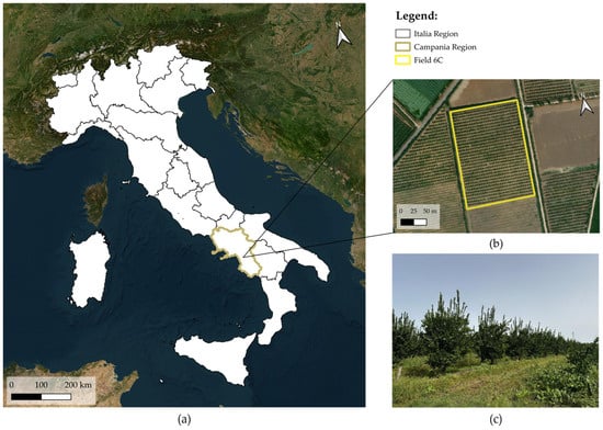
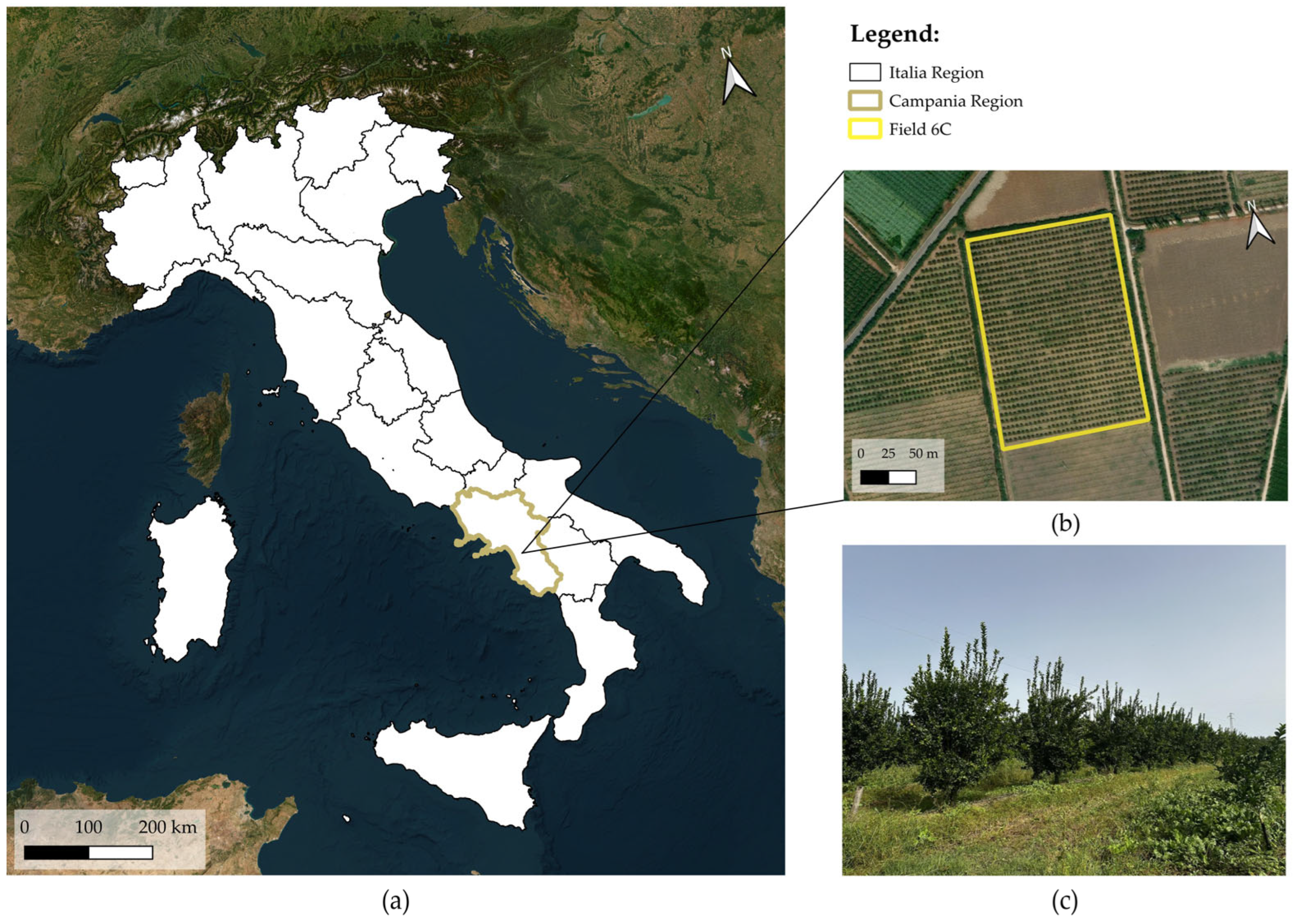
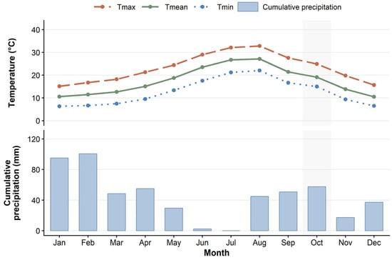
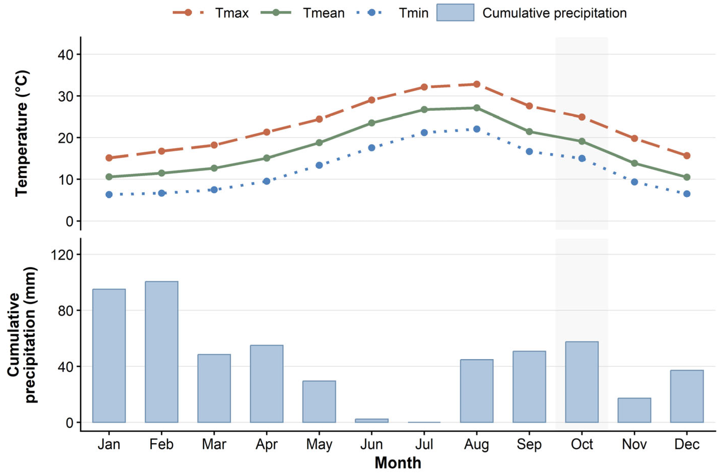
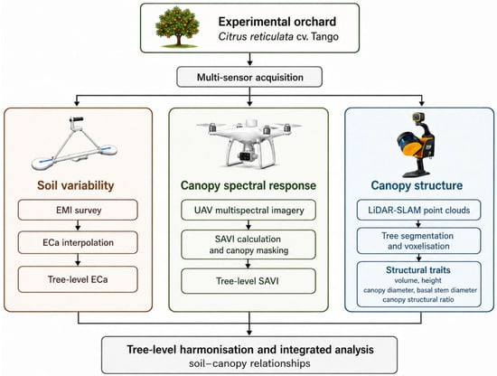
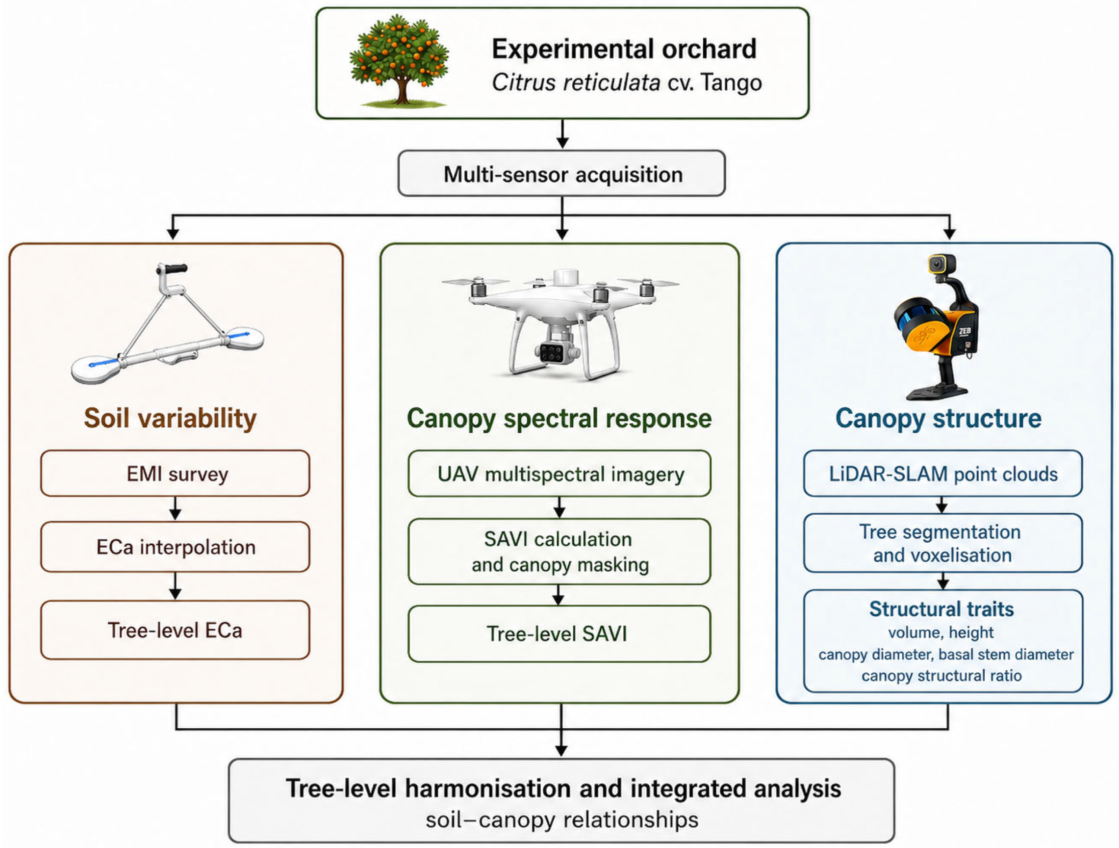
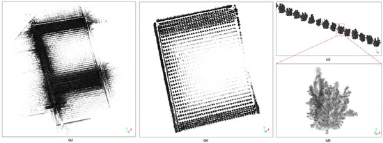
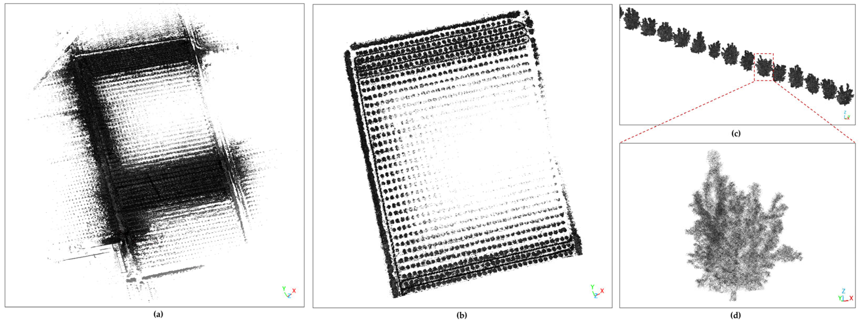
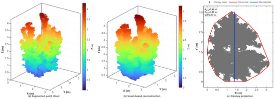
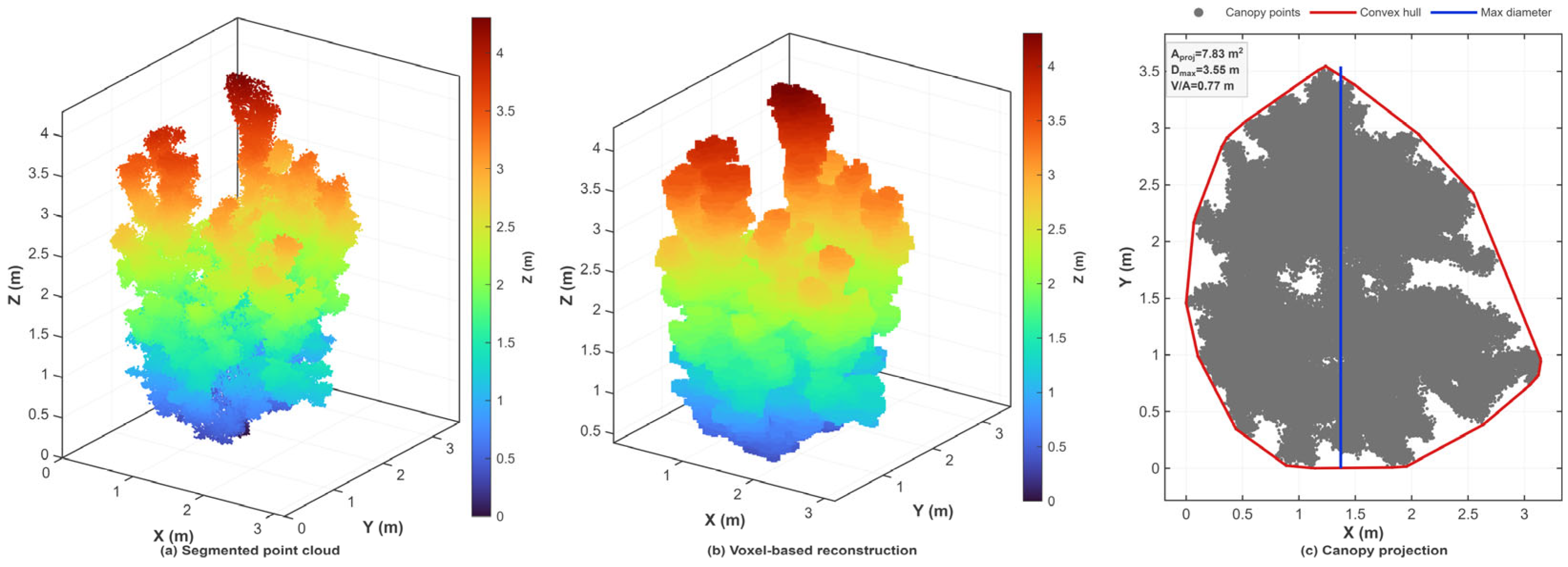
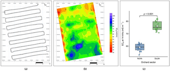
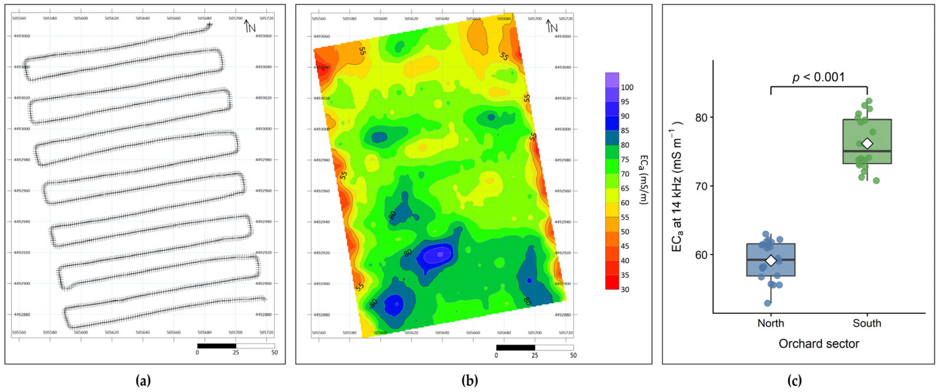
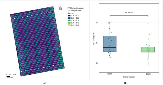
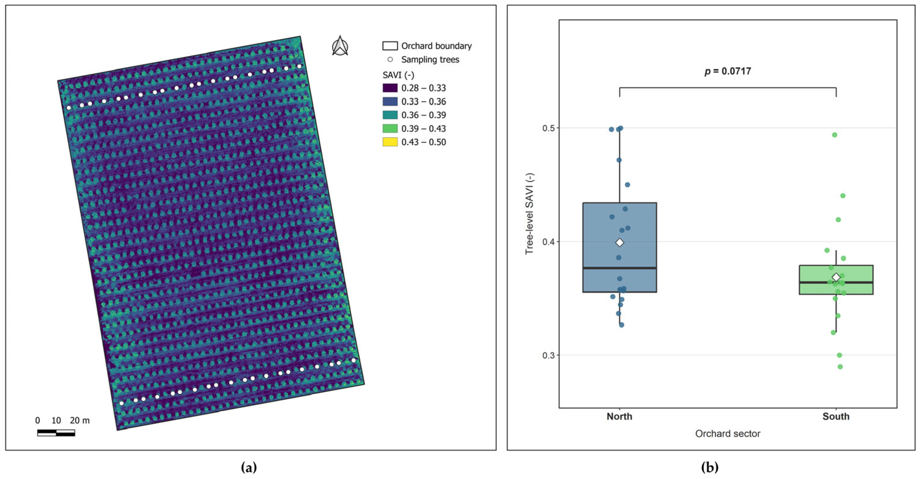
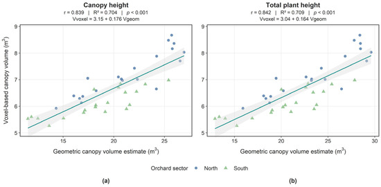
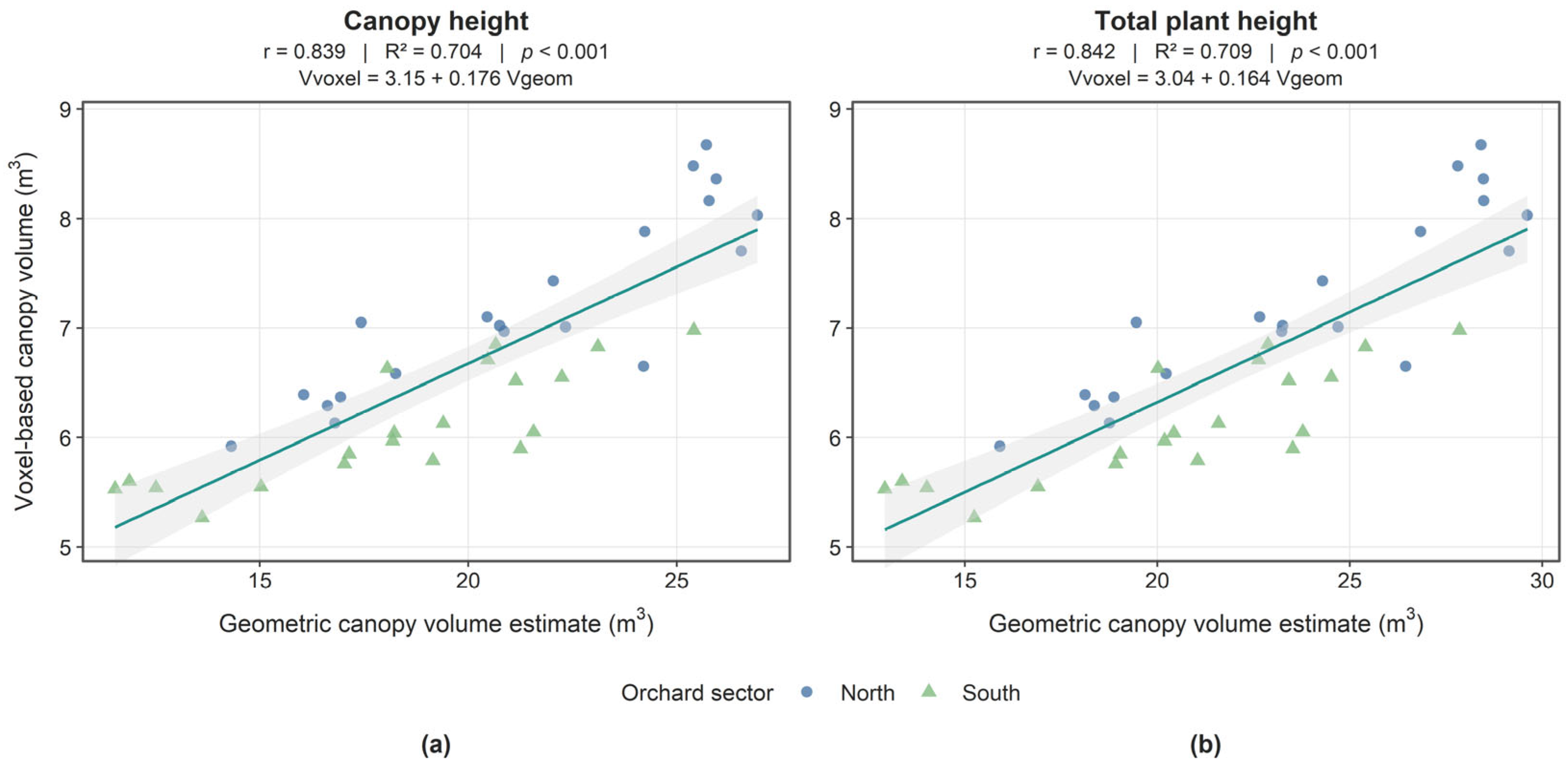
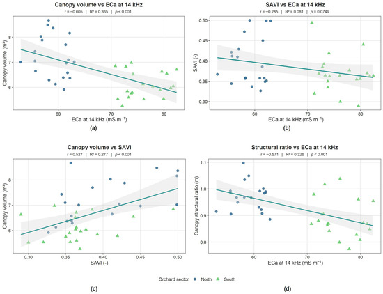
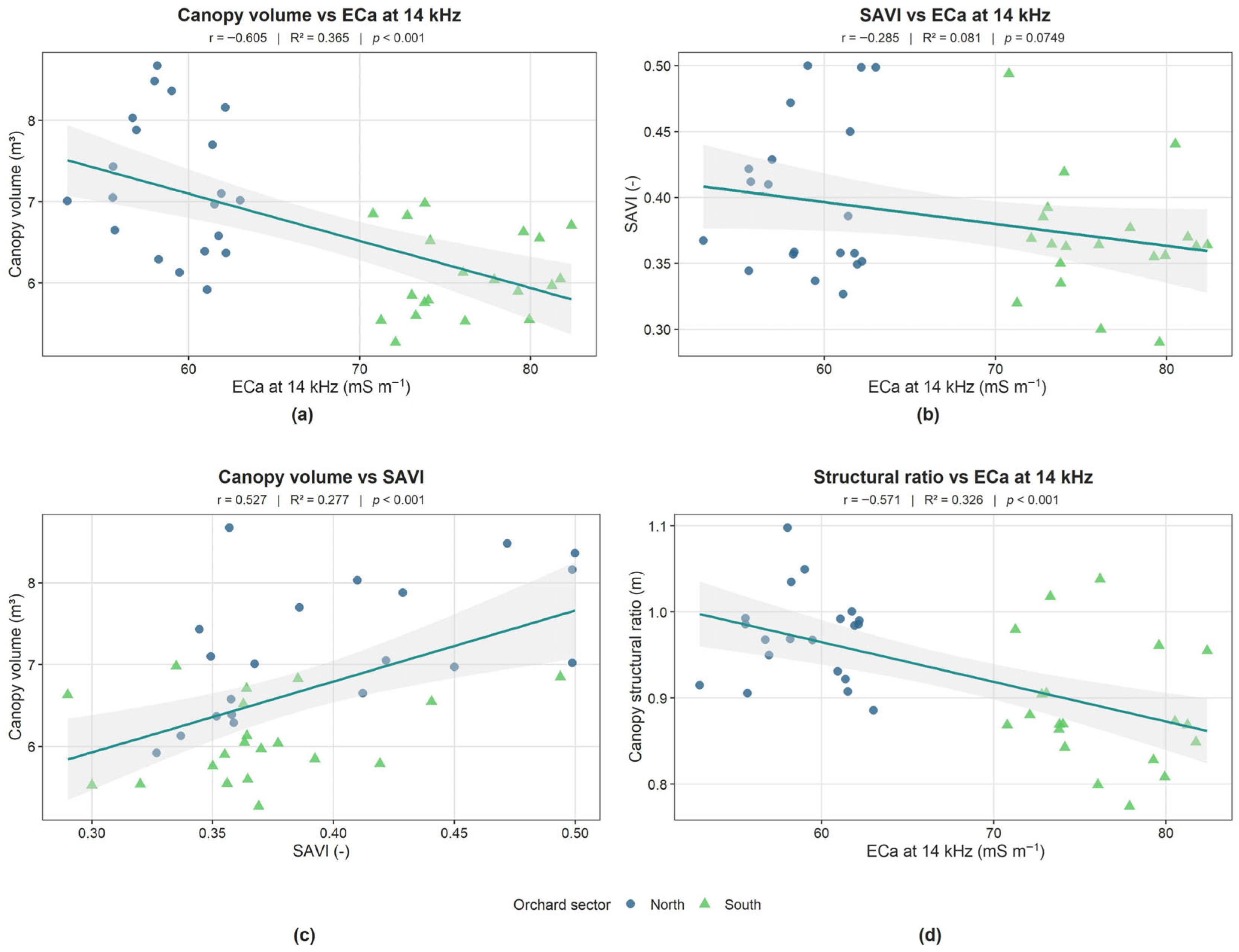
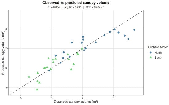
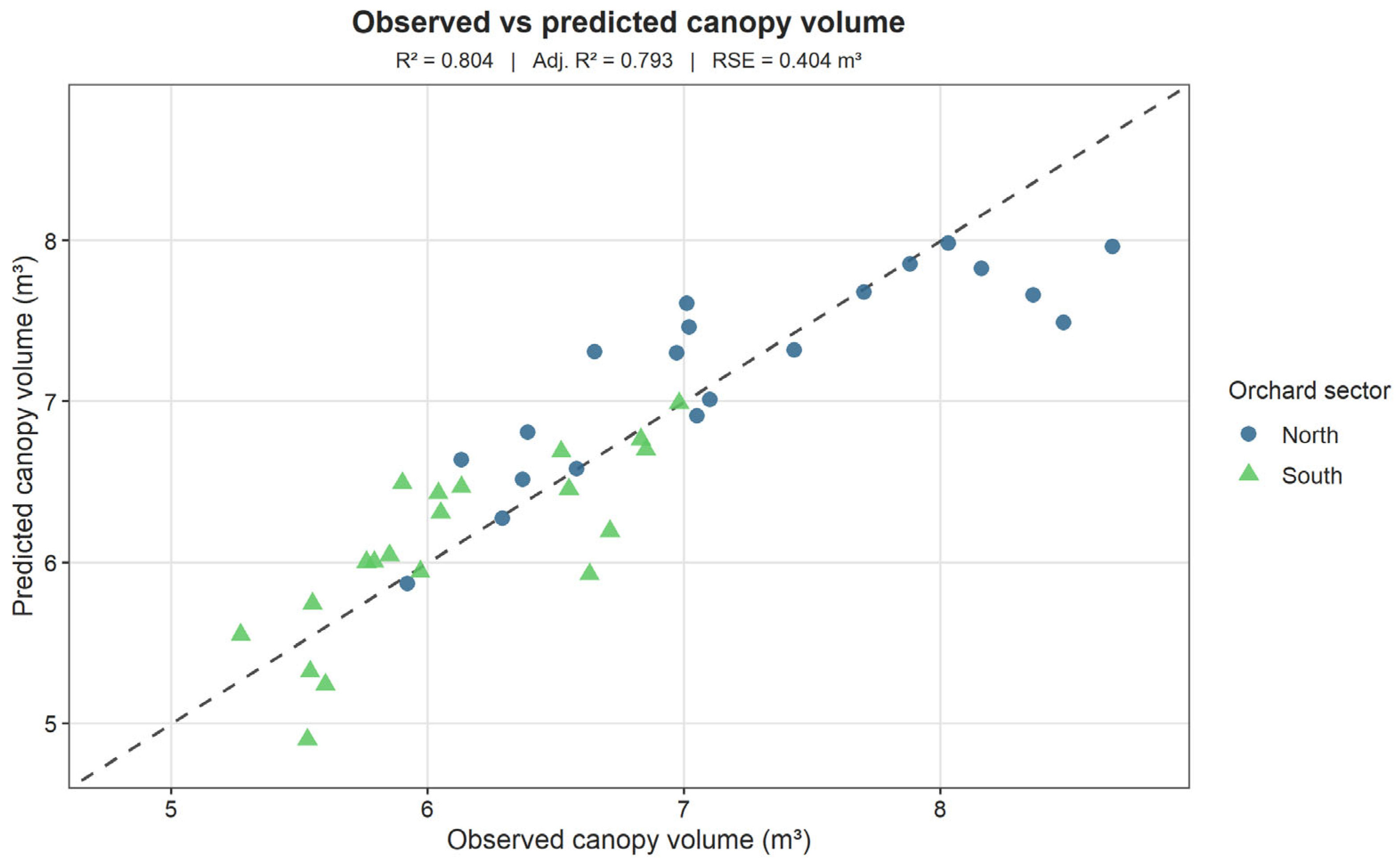
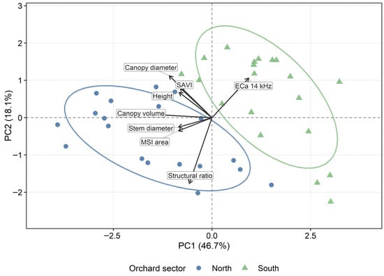

Disclaimer/Publisher’s Note: The statements, opinions and data contained in all publications are solely those of the individual author(s) and contributor(s) and not of MDPI and/or the editor(s). MDPI and/or the editor(s) disclaim responsibility for any injury to people or property resulting from any ideas, methods, instructions or products referred to in the content. |
© 2026 by the authors. Licensee MDPI, Basel, Switzerland. This article is an open access article distributed under the terms and conditions of the Creative Commons Attribution (CC BY) license.