Navigation System for Intelligent Harvester Based on Tightly Coupled Adaptive Fusion and Cooperative Control

Abstract

Autonomous navigation of harvesters in hilly and mountainous terrain faces two major challenges: sensor discrepancies among multiple sources and depth distortion caused by terrain slopes. This paper proposes a tightly coupled vision–inertial–depth navigation and control system to address these issues. The system fuses visual features with inertial data within an adaptive extended Kalman filter framework that dynamically adjusts sensor weights to resolve conflicts from illumination changes and inertial drift. It also incorporates a real-time depth compensation model based on vehicle attitude to correct spatial mapping distortions during slope operations. Additionally, a multi-controller coordination strategy integrates steering, speed, and header height to align state estimation with control execution. Field experiments show that the system achieves a lateral positioning error of 3.4 cm—48.5% and 81.5% lower than pure-vision and pure-inertial approaches, respectively-and remains within 9.5 cm even in degraded scenarios. These results demonstrate the system’s ability to deliver high-precision navigation and stable operation on complex terrain.

1. Introduction

Hilly and mountainous farmland accounts for approximately 30% of China’s arable land, presents undulating terrain, irregular crop rows, and frequent GNSS signal loss, severely constraining the performance of conventional navigation systems. On compact harvesters, single-sensor solutions exhibit a pronounced “bottleneck effect”: RTK-GNSS loses signal over 30% in orchards and valley slopes [1]; pure vision misdetects over 60% under illumination changes or lodged crops [2]; and inertial navigation drifts at 0.3°/min without periodic correction [3]. These compounded limitations motivate multi-sensor integration, yet existing fusion approaches are ill-equipped for hilly agricultural scenarios. Early loosely coupled GNSS/INS architectures fail under intermittent satellite visibility [4]; more recent tightly coupled visual–inertial odometry frameworks such as VINS-Mono [5] and OKVIS [6], though accurate in urban environments, have not been systematically tailored to the specific disturbances of hilly farmland—extreme light fluctuation, sparse and irregular crop textures, and frequent attitude changes induced by slopes. Adaptive Kalman filters [7] typically treat adaptation as a binary switch rather than a continuous, multi-modal weighting strategy that accounts for simultaneous degradation of vision and GNSS. Moreover, none of these methods incorporate real-time vehicle attitude to compensate for depth distortion caused by pitch and roll on slopes [8], a critical issue that directly affects obstacle detection and header height control.

These limitations define three specific technical bottlenecks for harvester navigation in hilly terrain: (1) lack of an adaptive fusion framework that dynamically balances vision, IMU, and GNSS according to their instantaneous reliability; (2) absence of a geometry-based depth correction model that uses instantaneous attitude to undo slope-induced perceptual distortion; and (3) disconnection between state estimation and multi-actuator control (steering, speed, header), which prevents terrain-aware coordination. To break these bottlenecks, this paper proposes a tightly coupled vision–inertial–depth navigation and control system with three corresponding innovations: an extended Kalman filter with adaptive weighting (0.5–1.0) and hysteresis for smooth modal transitions, a real-time depth compensation model that utilises IMU pitch/roll to correct slope-induced spatial mapping errors, and a two-layer online rolling optimisation architecture that collaboratively adjusts steering, speed, and header height controllers. The proposed system is validated through comprehensive field trials under diverse conditions, demonstrating its capacity for high-precision, robust navigation on complex hilly terrain.

2. Materials and Methods

2.1. Experimental Platform and System Architecture

This study employed a self-developed compact mountainous terrain harvester as the experimental platform to validate the proposed methodology. The technical specifications of the harvester are detailed in Table 1.

Table 1. Technical parameters of harvester.

Item	Data	Unit
Overall Dimensions	3800 × 1660 × 2480	mm
Machine Weight	1200	kg
Header Working Width	1350	mm
Rated Feed Rate	1.5	kg/s
Operating Speed	0.6–2.0	m/s
Track Gauge	710	mm

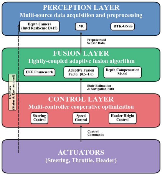
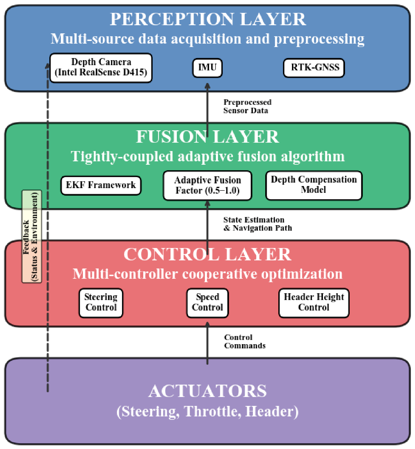
The overall architecture of the high-precision navigation system proposed in this study is illustrated in Figure 1. It adopts a hierarchical progressive design philosophy [9], comprising three levels: the perception layer, the fusion layer, and the control layer. Information exchange and decision optimization [10] are achieved through a tightly coupled approach.

Figure 1. System overall architecture.

System Architecture Overview:

(1) Perception Layer: It is responsible for acquiring and pre-processing multi-source raw data, including visual information, inertial data, satellite positioning information, and environmental depth information.

(2) Fusion Layer: Receives data from the perception layer and, through tightly coupled adaptive fusion algorithms, outputs high-precision, high-reliability estimates of the vehicle’s global position, velocity, and environmental depth.

(3) Control Layer: It generates steering, throttle/brake, and header hydraulic lift control commands based on the state information and navigation targets output by the fusion layer. This is achieved through a multi-controller collaborative optimisation strategy, driving the vehicle to execute the required manoeuvres.

2.2. Perception Layer Hardware Configuration and Data Preprocessing

2.2.1. Visual Perception Unit

This study utilized the Intel RealSense D415 depth camera, which is based on structured light stereo technology and combines active infrared projection with a stereo matching mechanism [11]. It can reliably capture depth information even under low-light or no-light conditions, making it particularly suitable for low-light environments such as overcast days and dusk in hilly areas, thereby ensuring the reliability of crop detection. The camera features high precision and strong resistance to interference, significantly reducing the impact of fluctuations in ambient light. During installation, the camera was mounted 2.1 m above the ground to avoid obstruction by low-growing crops, and the pitch angle was adjusted to 30 degrees to balance near-field detail with far-field visibility. The dataset consists of manually collected images of hilly paddy field scenes, annotated using LabelImg (version:1.8.6). The camera’s depth measurement range is 0.3 m to 10 m, with a colour image resolution of 1920 × 1080 and a depth image resolution of 1280 × 720. Mounted on a small combine harvester, data was collected during three time periods: early morning, midday (under strong sunlight), and dusk. The original dataset contained 593 images. To enhance data diversity and better align with real-world applications, each original image underwent data augmentation, including linear contrast enhancement, Gaussian noise addition, and horizontal flipping, ultimately expanding the dataset to 2372 images. The dataset was split into training, validation, and test sets in a 7:2:1 ratio. Annotated classes include field ridges, harvested areas, obstacles, areas with slight lodging, harvesters, people, unharvested areas, and inter-row spaces.

The experiment was conducted on Windows 11 using the PyTorch (version: 2.0.1) framework and CUDA 10.2. The hardware configuration consisted of an i7-13650HX CPU and an RTX 4060 GPU. Training was performed using the YOLOv8n-seg model with a batch size of 8 and 8 threads. The training ran for 300 iterations with early stopping set at 100 iterations, using loss weights of cls: 0.5 and box: 7.5, mask: 2.5, input resolution 640 × 640, learning rate 1 × 10⁻³ (cosine annealing), AdamW optimizer (β1 = 0.9, β2 = 0.999), weight decay 5 × 10⁻⁴, gradient clipping norm: 10.0, inference frame rate reaching 32 FPS, with all other parameters set to default.

To ensure depth perception accuracy, this research employs post-processing on raw depth maps captured by the depth camera. A hybrid filtering algorithm [12] combining median filtering with morphological closing operations effectively suppresses abnormal depth value fluctuations and noise caused by field interference. Concurrently, the system incorporates a dynamic confidence check mechanism based on historical frames. Should the proportion of valid depth pixels in the current frame fall below a preset threshold (e.g., 40%), that frame is automatically discarded. Valid data from the preceding frame is then used for interpolation compensation, further safeguarding data continuity under extreme lighting conditions (such as strong backlighting).

The calibration process employs the Kalibr toolbox for joint calibration of the stereo cameras and IMU, primarily calibrating the cameras’ intrinsic and extrinsic parameters alongside the IMU’s noise parameters (including white noise and zero bias instability of accelerometers and gyroscopes). The tables of the cameras’ intrinsic and extrinsic parameters are shown in Table 2. These data form the foundation for ensuring visual perception accuracy and depth measurement precision, thereby guaranteeing spatio-temporal synchronisation. The depth scale factor was calibrated using a planar checkerboard fitting method, achieving an error rate below 0.5%. To address temperature drift, the system automatically recalibrates every 10 min to maintain stability. To address the issue of temperature drift, the system incorporates a background asynchronous recalibration mechanism: calibration is automatically triggered every 10 min, and this process runs in a separate thread without blocking the main control loop. During recalibration, the system continues to use the calibration parameters from the previous cycle for navigation and control. Once the new calibration parameters are generated, they are gradually updated in the fusion module using first-order low-pass filtering (smoothing coefficient γ = 0.2) to prevent control oscillations caused by sudden parameter changes. In actual testing, a single background recalibration took approximately 80 ms (based on 20 pre-acquired frames of static checkerboard images), which is far less than the allowable margin of the control cycle (100 ms), and the increase in CPU utilization was less than 5%. Therefore, this process has no perceptible impact on real-time navigation and harvesting operations.

Table 2. Internal and external parameters of depth cameras.

Parameter	Colour Camera	Infrared Camera	Unit	Remarks
Focal length	fx = 628.18, fy = 627.23	fx = 1087.59, fy = 1094.61	Pixel	-
Principal point (Cx,Cy)	(295.35, 230.46)	(640.0, 360.0)	Pixel	IR primary point manually corrected to image centre
Radial distortion	k1 = −0.0711, k2 = 0.3734	k1 = −0.9209, k2 = 10.0156	-	-
Tangential distortion	p1 = 0.001, p2 = −0.0005	p1 = 0.002, p2 = −0.001	-	Default value
Higher-order radial distortion	k3 = 0.0	k3 = 0.0		Default value
Reprojection error	0.029	0.055	Pixel	-
Rotation matrix (R)	[0.998, 0.012, −0.061, −0.015, 0.999, 0.043, 0.060, −0.044, 0.997]		-	3 × 3 matrix, after mean filtering
Translation vector (T)	[54.7, −1.2, 3.8]		mm	Z-axis corrected to physical baseline 55 mm
Baseline length	54.7		mm	Calculated based on translation vector model length
Global scaling factor	1.0436		-	-
Non-linear compensation segment factor	$\mathrm{Z}={\displaystyle \frac{54.5\times 628.18}{\mathrm{d}}}$		-	-

After the sensors were calibrated and installed, the real-time performance and accuracy of the multi-sensor data fusion were verified. Through field simulation tests, GNSS positioning data, IMU attitude information, and visual depth data were collected under various operating conditions.

Experimental results show that the fusion-based positioning accuracy improved by 35% compared to single-GNSS systems, with attitude angle errors consistently maintained within 0.5°, meeting the high-precision standards for environmental perception required in unmanned operations. When the visual sensors detect a deviation from the crop boundary, IMU and GNSS data rapidly supplement the positioning information. The system generates steering adjustment commands within 0.2 s, with electric actuator response delays of less than 0.1 s. This seamless integration of perception and execution provides a robust hardware foundation for the operation of subsequent intelligent operation systems.

2.2.2. Inertial Measurement Unit (IMU)

The IMU is mounted near the vehicle’s centre of gravity via a dedicated aluminium alloy shock-absorbing bracket. Its mounting coordinate system (X-forward, Y-leftward, Z-vertical) is precisely aligned with the vehicle coordinate system, minimising the impact of mounting errors on attitude calculation. To address the extreme temperature fluctuations encountered during agricultural machinery operations, the system employs an online zero bias compensation strategy based on a temperature lookup table [13]. A zero bias-temperature lookup table is established through high- and low-temperature calibration of the IMU prior to shipment. During operation, the system continuously monitors the core temperature of the IMU and dynamically compensates for the zero bias of the accelerometer and gyroscope, reducing attitude errors caused by temperature drift by approximately 60%. Performance parameters are shown in Table 3.

Table 3. IMU Performance Parameters.

Item	Data
Attitude accuracy	Roll/Pitch: <0.2° rms
Update rate	Heading: <0.3° rms
Gyro range	100 hz
Accelerometer range	±500°/s
Accelerometer zero bias stability	4 deg/h @1σ
Position estimation accuracy	<2% @1σ

2.2.3. Positioning Unit

The RTK-GNSS system communicates with its self-built reference station via 4G networks, maintaining a stable communication latency of 50–100 ms. To mitigate multipath effects prevalent in hilly terrain, the system employs GNSS modules equipped with multipath-resistant antennas. These modules apply weighting adjustments based on satellite observation signal-to-noise ratio (SNR) values [14], significantly enhancing positioning accuracy and fix rates within complex signal environments such as orchards and sloping landscapes.

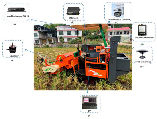
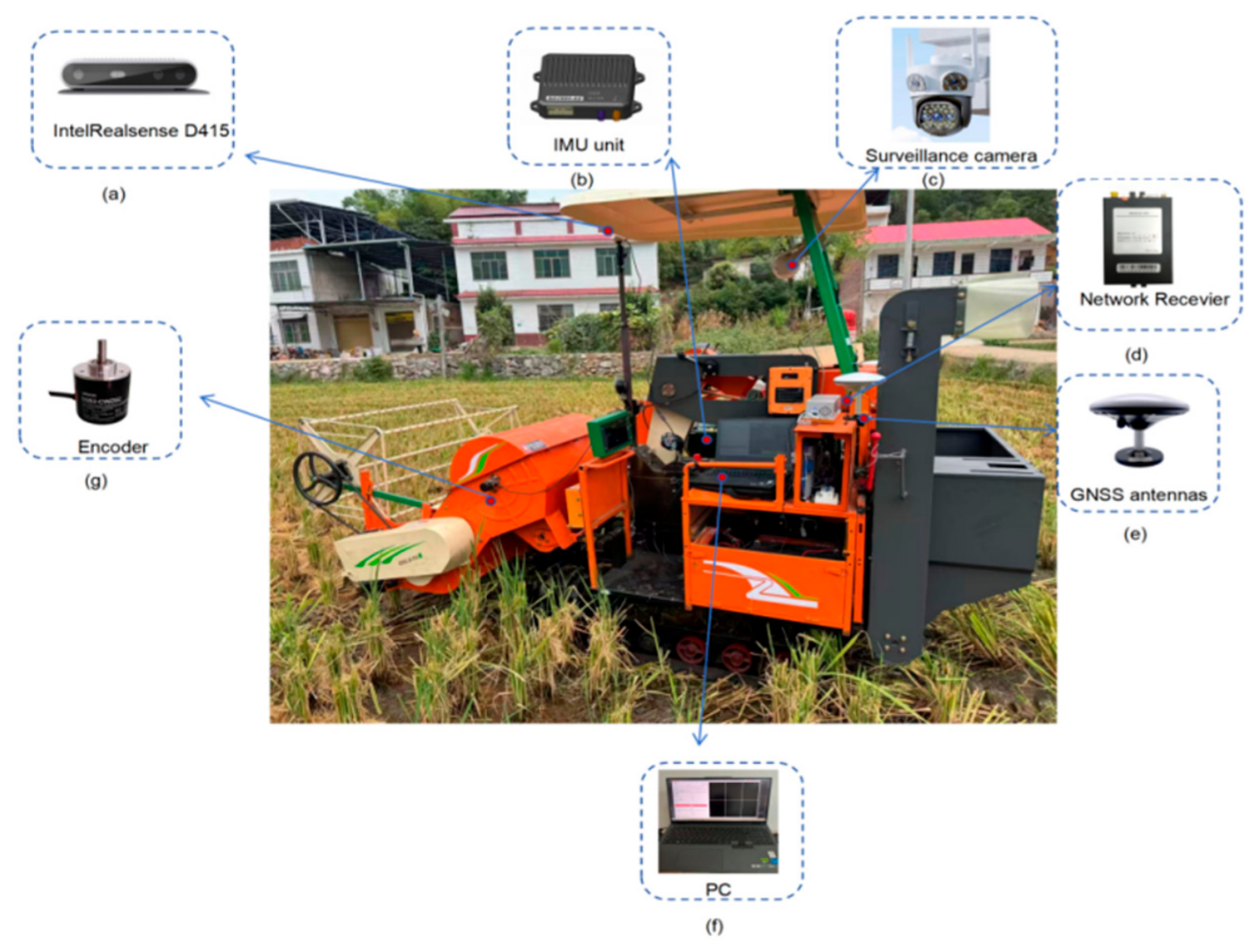
RTK-GNSS dual-antenna configuration (1 m baseline), multi-system support, and signal redundancy strategy. RTK-GNSS performance parameters are detailed in Table 4, with installation locations shown in Figure 2. Furthermore, the figure clearly marks the mounting positions of key components including the depth camera, IMU, GNSS antenna, and industrial PC, providing an intuitive overview of the system’s hardware integration solution.

Table 4. RTK-GNSS performance parameters.

Item	Installation Location	Indicator	Data
RTK-GNSS	Both sides of the vehicle	Dual-antenna positioning accuracy (RMS)	0.1° per metre baseline
		Speed Accuracy (RMS)	0.03 m/s
		PPS accuracy (RMS)	20 ns
		Refresh rate	20 hz
		RTK initialisation time	<5 s

Figure 2. Whole equipment: (a) IntelRealsense D415, (b) IMU unit, (c) Surveillance camera, (d) Network Receiver, (e) GNSS antennas, (f) PC, (g) Encoder.

2.3. Tightly Coupled Adaptive Fusion Algorithm

2.3.1. EKF-Based Fusion Framework

To achieve tight-coupled fusion of depth cameras, RTK-GNSS, and IMU, this paper employs the Extended Kalman Filter (EKF) as the core framework for multi-source sensors fusion. The system’s state vector $x_k$ encompasses the harvester’s position, velocity, and attitude within the global coordinate system, alongside the IMU’s zero-bias error. The specific model is as follows:

State equation:

$$x_k=F_{k-1}{x}_{k-1}+B_{k-1}{u}_{k-1}+w_{k-1}$$

(1)

Among these, $x_k$ denotes the state vector, specifically defined as

(1)

$x={\left[p_x,p_y,p_z,v_x,v_y,v_z,q_w,q_x,q_y,q_z,b_a^x,b_a^y,b_a^z,b_g^x,b_g^y,b_g^z\right]}^T$;

(2)

$\left[p_{x,}{p}_{y,}{p}_z\right]$ and $\left[v_{x,}{v}_{y,}{v}_z\right]$ denote the vehicle’s position and velocity in the global coordinate system, respectively;

(3)

[$q_w,q_x{q}_y,q_z$] represents the quaternion of the vehicle’s body attitude, $q_w$ is the real part, and ($q_x$, $q_y$, $q_z$) is the imaginary part, satisfying the normalization constraint ${q_w}^2+{q_x}^2$ + ${q_y}^2$ + ${q_z}^2$ = 1;

(4)

[$b_a^x,b_a^y,b_a^z$] and [$b_g^x,b_g^y,b_g^z$] denote the zero bias errors of the accelerometer and gyroscope, respectively; $F_{k-1}$ is the state transition matrix, $B_{k-1}$ is the control input matrix, $u_{k-1}$ is the control input, and $w_{k-1}$ is the process noise [15], assumed to be white Gaussian noise [16].

Observation equation:

$$z_k=H_k{x}_k+v_k$$

(2)

Here, $z_k$ denotes the observation vector, whose values originate from multiple sensors: relative pose changes provided by the visual odometer, absolute position and heading supplied by RTK-GNSS, and the relative distance between the vehicle and crop rows delivered by the compensated depth camera. $H_k$ represents the observation matrix, while $v_k$ signifies the observation noise. In this paper, the EKF state vector has 16 dimensions, and the observation vector $z_k$ has 10 dimensions, including the 6-dimensional pose increments from the visual odometry, the 3-dimensional position from RTK-GNSS, and the 1-dimensional lateral offset from the depth camera. The corresponding observation matrix $H_k$ is a 10 × 16 Jacobian matrix. Time synchronization uses the RTK-GNSS PPS pulse (accuracy: 20 ns) as the primary clock reference. Both IMU (100 Hz) and visual (30 Hz) data are aligned to this reference, and visual and IMU data are synchronized to the visual frame acquisition time via linear interpolation. The overall system latency is 60–80 ms, meeting real-time requirements.

2.3.2. Adaptive Fusion Factor Design

$$a_{\mathrm{k}}={\displaystyle \frac{{\sigma }_{IMU}^2}{{\sigma }_{IMU}^2+{\sigma }_{\mathrm{Visual}}^2}}$$

(3)

Here, ${\alpha }_k$ denotes the adaptive fusion weight, ranging from [0, 1]. In this study, the lower limit is set to 0.5. The primary objective is to ensure that, even when visual data is completely lost (α → 0), at least 50% of the weight is still assigned to the IMU. This is because the drift rate of pure IMU integration is approximately 0.3°/min, allowing it to maintain usable accuracy for a short period. However, if α is too low (<0.5), the EKF will excessively suppress the IMU prediction, and once the visual data undergoes a sudden change, the localization solution will experience uncontrollable abrupt changes. While ${\sigma }_{IMU}^2$ and ${\sigma }_{Visual}^2$ represent the variance estimates of the IMU and visual sensor observations at the current time step, respectively. ${\sigma }_{Visual}^2$ estimated using a sliding window (window size W = 20 frames) to reflect the stability of recent visual pose estimates. ${\sigma }_{IMU}^2$ fixed at (0.05 m)² based on the device’s nominal value, Equation (3) is derived from the classic variance-weighted method of the EKF. This paper does not alter its theoretical core but instead implements two engineering improvements tailored to the combine harvester operating scenario: (1) First-order low-pass smoothing (β = 0.3) is applied to the output of Equation (3) to prevent abrupt changes in the weights; (2) A hysteresis switching logic was designed: weight switching is triggered when ${\sigma }_{Visual}^2$ exceeds the preset threshold (${\tau }_{low}$ = 0.025 m² is the low-to-high switching threshold, and ${\tau }_{high}$ = 0.045 m² is the high-to-low switching threshold), the intermediate region maintains the previous state. The measured modal switching frequency was reduced from 0.8 Hz to 0.12 Hz.

To further incorporate RTK-GNSS signal quality into weighted decision-making, let $q_k^{gnss}$ ∈ [0, 1]. Based on a comprehensive assessment of the real-time solution status, the number of visible satellites, and the average signal-to-noise ratio: When the solution state is “Fix,” the number of visible satellites is ≥12, and the average signal-to-noise ratio is >40 dBHz, q = 1; q decreases in stages as signal quality deteriorates, and q = 0 when the lock is lost. The GNSS observation weight is set to ${{\alpha }_k^{gnss}=0.5\cdot q}_k^{gnss}$, while the visual and IMU weights are allocated within the remaining weight space according to Equation (3). This design ensures that when GNSS loses lock (q = 0), the system automatically switches to a tightly coupled visual-IMU mode, maintaining navigation continuity even during intermittent satellite signal interruptions.

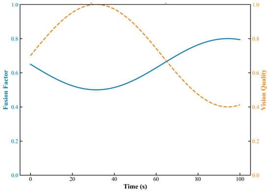
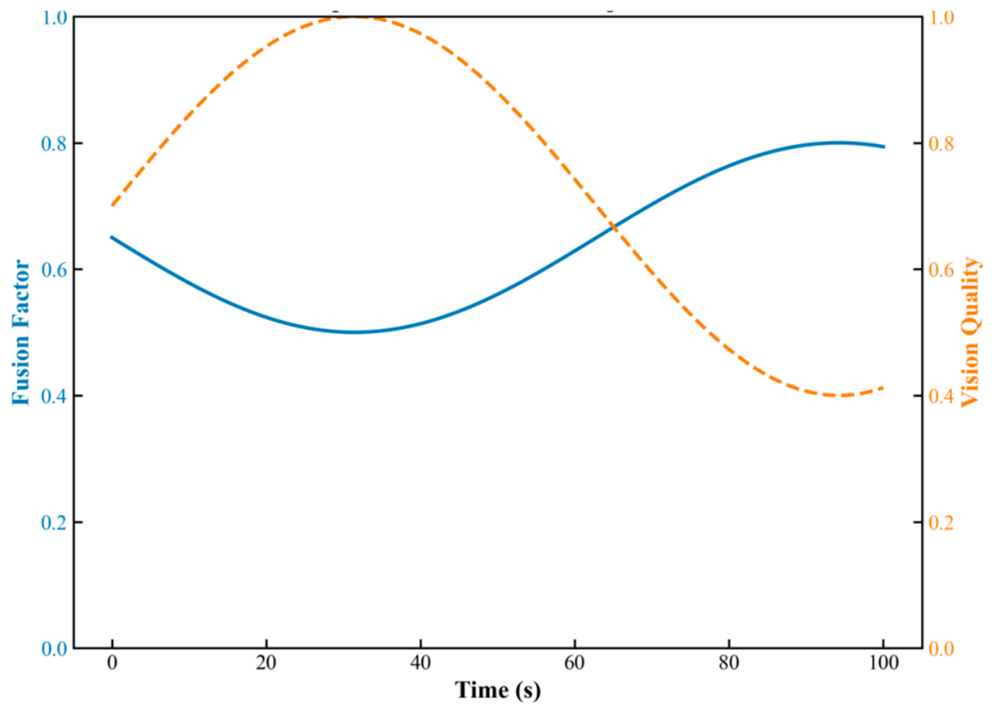
The factor ${\alpha }_k$ is introduced into the observation update stage of the EKF to adjust the observation noise covariance matrix. When visual information quality is high, ${\sigma }_{Visual}^2$ decreases and ${\alpha }_k$ approaches 1, leading the system to place greater trust in visual observations. When visual degradation occurs, ${\sigma }_{Visual}^2$ increases and ${\alpha }_k$ decreases, causing the system to automatically switch to IMU-dominant mode. This effectively prevents jumps and divergence in the positioning solution. As shown in Figure 3, the adaptive fusion factor ${\alpha }_k$ dynamically adjusts in response to changes in visual observation variance—when the variance increases (such as in the event of occlusion or sudden changes in lighting), the fusion factor automatically increases, and the system smoothly transitions from “vision-dominated” to “IMU/GNSS-dominated” mode, thereby ensuring the continuity and robustness of positioning.

Figure 3. Adaptive fusion factor adjustment.

To illustrate the above mechanism intuitively, consider the scenario where the harvester moves from an open field into a shaded area under tree canopy: the number of visual feature points drops sharply from approximately 200 to fewer than 80, and the visual odometry covariance increases from about 0.015 m² to above 0.045 m² within 0.5 s. Upon detecting that ${\sigma }_{Visual}^2$ exceeds the threshold ${\tau }_{\mathrm{h}\mathrm{i}\mathrm{g}\mathrm{h}}$, the fusion factor ${\alpha }_k^{vis}$ gradually decreases from 0.85 to 0.50 through the smoothing filter, while the GNSS weight remains at 0.40 (with good signal quality) and the IMU weight correspondingly increases from 0.15 to 0.50. Throughout this process, the positioning output exhibits no jumps, and the lateral error remains consistently within 5 cm. This example clearly demonstrates the automatic response and smooth transition capability of the adaptive fusion factor under sudden changes in visual quality.

2.3.3. Dynamic Pose-Based Depth Compensation Model

To address the issue of severe distortion in depth camera measurements caused by vehicle pitch and roll during operations in hilly terrain, this paper treats depth distortion as a 3D spatial rotation problem. Let the raw point coordinates output by the depth camera be $P_{cam}=(x_c,y_c{,z}_c{)}^T$. Here, $z_c$ is the depth value along the optical axis. The vehicle’s pitch angle $\mathsf{\theta }$ and roll angle $\mathsf{\varphi }$ are output in real time by the EKF fusion layer (see Table 3). The projection transformation from the camera coordinate system to the horizontal world coordinate system is given by:

$$P_{\mathrm{world}}=R_{\mathrm{y}}\left(\theta \right)\cdot R_x(\varphi )\cdot P_{cam}$$

(4)

Here, $R_y\left(\theta \right)$ and $R_x\left(\varphi \right)$ are the rotation matrices about the Y-axis and X-axis, respectively. After expansion, the true vertical height is:

$$z_{corrected}=-x_c\sin \theta +y_c\sin \varphi \cos \theta +z_c\cos \varphi \cos \theta$$

(5)

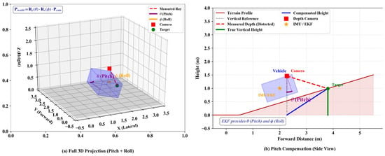
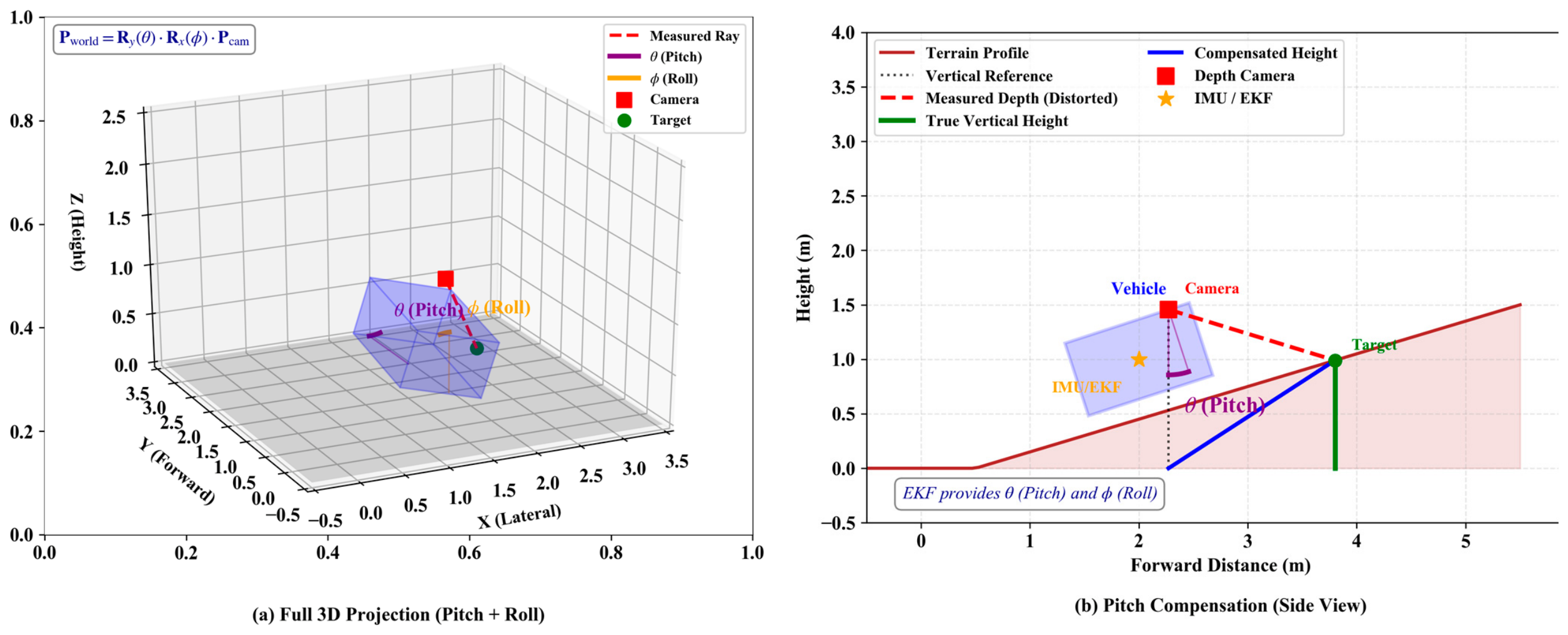
Equation (5) simultaneously compensates for the full rotational effects of pitch and roll, ensuring that the lateral projection coordinates x and y are corrected in unison, thereby avoiding projection distortion of crop row positions during operations on sloped terrain. This model assumes that the depth camera is rigidly mounted on the harvester’s chassis and that the relative transformation between the camera and the IMU has been pre-calibrated (see Table 2). Figure 4 illustrates the principle of slope-based depth-aware distortion and the EKF-based attitude compensation method. Figure 4a depicts the distortion in depth measurements on sloped terrain, while Figure 4b shows the depth model after attitude compensation.

Figure 4. Depth distortion and IMU compensation for slope operation: (a) Measurement distortion; (b) Compensated depth model.

Figure 4a illustrates the issue of geometric distortion in depth camera measurements caused by vehicle pitch and roll during operations on sloping terrain; Figure 4b demonstrates how the real-time pitch angle ${\theta }_{EKF}$ and roll angle ${\varphi }_{EKF}$, estimated by the EKF fusion layer, correct the raw 3D point $P_{cam}=(x_c,y_c{,z}_c{)}^T$ through rigid-body rotation projection, yielding the corrected coordinates including the true vertical height $z_{corrected}$, thereby providing precise environmental perception data for core control systems.

2.4. Multi-Controller Collaborative Optimisation Strategy

The navigation control of intelligent harvesters constitutes a complex multivariate coupling problem [17]. Steering control impacts path-tracking accuracy; speed control must balance operational efficiency with terrain safety; while header height control directly affects harvesting quality and equipment safety. These three elements interact: excessive speed causes steering lag and insufficient header adjustment; during slope turns, vehicle tilt further affects the header’s actual height. Consequently, traditional independent PID controllers struggle to achieve globally optimal performance.

Strong coupling exists between steering, speed, and header height control, necessitating coordinated optimisation to achieve precise path tracking and stable operation.

2.4.1. Collaborative Optimisation Architecture

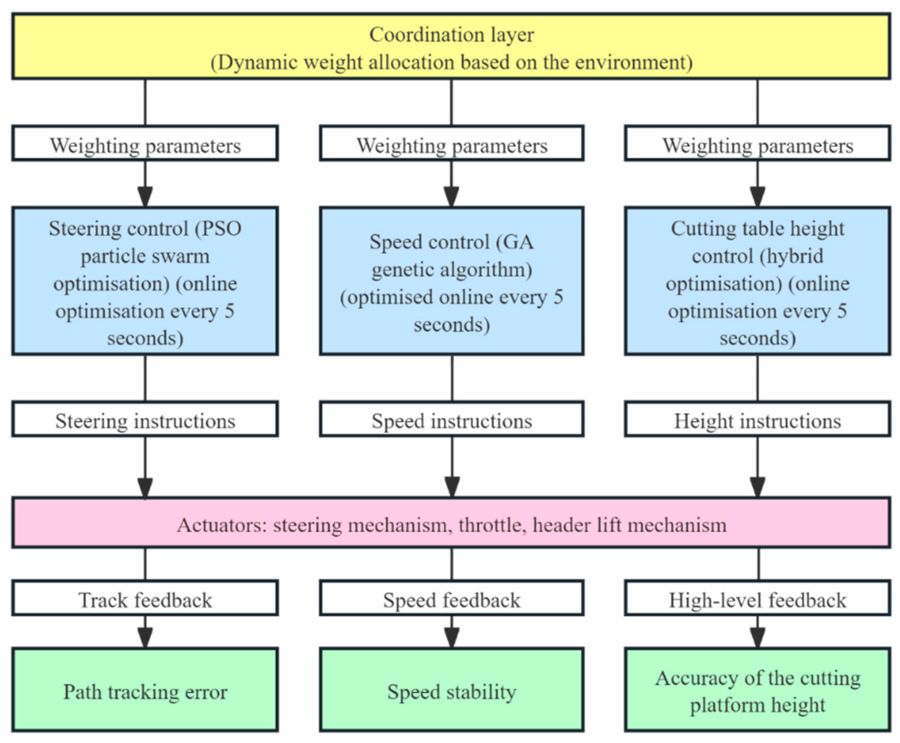
Upper Layer (Coordination Layer): Responsible for dynamically calculating and allocating the optimisation weights across three subsystems—steering control, speed control, and header height control—based on real-time field environmental data (terrain gradient, operating speed, depth information, etc.) and global operational objectives.

Lower Layer (Optimisation Layer): For each control subsystem (steering, speed, header height), employs an online rolling optimisation strategy. The optimiser (improved PSO/GA) runs every 5 s, utilising the latest sensor data to generate an optimal set of control parameters for that subsystem (e.g., ${\mathrm{K}}_{\mathrm{p}}$, ${\mathrm{K}}_{\mathrm{i}}$, ${\mathrm{K}}_{\mathrm{d}}$ for steering PID; corresponding parameters for speed PID; corresponding parameters for header height PID).

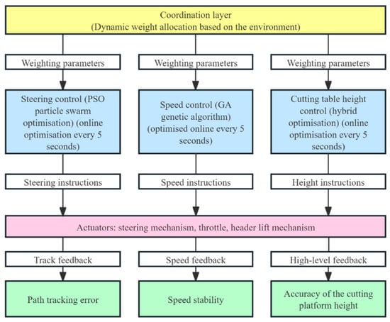
Finally, the optimised parameters are transmitted to the actuators, yielding tracking feedback for lateral error, feedback for speed stability, and accuracy feedback for header elevation. As illustrated in Figure 5, this diagram clearly depicts the complete workflow: the upper-layer coordinator allocates weights based on environmental information, the lower-layer optimiser performs online rolling parameter optimisation, and each controller receives optimised parameters to generate execution commands. This embodies the core concept for resolving multi-variable coupling problems.

Figure 5. Multi-controller collaborative optimization diagram.

2.4.2. Online Rolling Optimisation Process

This paper designs a periodic online rolling optimisation process that dynamically refreshes control parameters at five-second intervals. It aims to adapt in real time to dynamic changes in the agricultural environment and achieve global coordinated optimisation of steering, speed, and header height control. The core of the process lies in constructing and optimising a multi-objective fitness function, with the complete steps as follows:

(1) Real-time data acquisition: Every 5 s, the latest data is retrieved from the perception and fusion layers, including vehicle pose, speed, terrain gradient, depth information, and header height. At the start of each optimisation cycle, the system synchronously obtains the most recent data from both layers—encompassing global vehicle pose, current speed, terrain gradient, crop row depth information, and header height—to establish the foundational data for environmental assessment and optimisation calculations.

(2) Environmental Assessment and Weight Calculation: Based on current environmental parameters (e.g., slope), the weights (${\omega }_1,{\omega }_2,{\omega }_3$) for each sub-item within the multi-objective fitness function during the current optimisation cycle are calculated. This reflects differentiated emphasis on tracking accuracy, header stability, and control smoothness under varying operational conditions.

Multi-objective Fitness Function Construction and Interpretation: The fitness function serves as the optimiser’s evaluation criterion, designed to balance path tracking accuracy, operational quality, control smoothness, and safety. Its specific form is as follows:

$$J={\omega }_1\cdot {\displaystyle \frac{1}{N}}{\displaystyle {\displaystyle \sum _{i=1}^N}{e}_i^2}+{\omega }_2\cdot {\displaystyle \frac{1}{N}}{\displaystyle {\displaystyle \sum _{i=1}^N}{(h_i-h_{ref})}^2+}{\omega }_3\cdot {\displaystyle \frac{1}{N}}{\displaystyle {\displaystyle \sum _{i=1}^N}{\delta }_i^2}+P_{unsafe}$$

(6)

where: $e_i$ denotes the lateral tracking error at step i within the predicted time domain, serving to optimise path tracking accuracy; $h_i$ and $h_{ref}$ represent the actual and desired cutting height, respectively, minimising height fluctuations to ensure harvesting quality; ${\delta }_i$ represents the steering angle control variable, which penalises the control action itself to ensure smoothness in the control process and prevent actuator chattering; $P_{unsafe}$ denotes the safety penalty term, a step function that outputs an extremely large positive value (e.g., 10⁶) when any state or control variable (such as header height exceeding limits or steering angle surpassing thresholds) exceeds safe boundaries, otherwise returning zero. This mathematically enforces strict safety constraints on the optimisation results; N denotes the rolling optimisation window size, set to N = 10 (corresponding to 5 s) in this paper. (${\omega }_1,{\omega }_2,{\omega }_3$) represents the weighting coefficient determined in step (2), satisfying ${\omega }_1+{\omega }_2+{\omega }_3=1$. This function directly embodies the multi-objective optimisation targets of path tracking accuracy, operational quality, control smoothness, and safety. The weighting coefficients (ω₁, ω₂, ω₃) are determined in segments based on the slope θ: when θ < 3°, they are set to (0.7, 0.1, 0.2); when 3° ≤ θ ≤ 10°, they are determined by linear interpolation; and when θ > 10°, they are set to (0.3, 0.5, 0.2).

(3) Parameter Loading (Partitioned Parameter Library): To enhance optimisation efficiency and improve cold-start performance, the system queries and loads the historically optimal parameter set or parameter range for the current region from a pre-constructed partitioned parameter library, based on the global position provided by the RTK-GNSS. This serves as the initial point or search space constraint for the current optimisation iteration, reducing convergence time by approximately 40%. The zoning parameter library is divided into a 50 m × 50 m grid and indexed by RTK-GNSS position-mapped grid IDs. When called, if historical records exist for that grid, the historically optimal parameters are used as the centre of the PSO initial population (with the search range narrowed to ±20%); otherwise, the population is initialized randomly.

(4) Optimizer Execution: Using a lightweight version of the PSO optimization algorithm, within the specified parameter range and using the multi-objective fitness function determined in Step 2 as the evaluation criterion, the optimal parameter sets for the steering, speed, and header height controllers are determined for the current environment. The improved PSO employs linearly decreasing inertial weights (0.9 → 0.4), with 30 particles, a maximum of 50 iterations, c₁ = c₂ = 1.5, and a search space defined by Kp ∈ [0.5, 5.0], Ki ∈ [0, 2.0], and Kd ∈ [0, 1.0].

(5) Safety Constraints: During fitness function calculation, impose maximum penalty values on any control or state variables (e.g., steering angle, header height) exceeding preset safety limits, ensuring optimisation results strictly comply with operational safety requirements.

(6) Parameter Update and Application: The optimised parameter sets are updated into the corresponding controllers.

(7) Parameter Storage: The current optimal parameter sets, their fitness values, environmental parameters, and satellite position data are stored/updated in the partitioned parameter repository for subsequent optimisation and reference during operations in the same area.

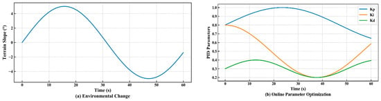
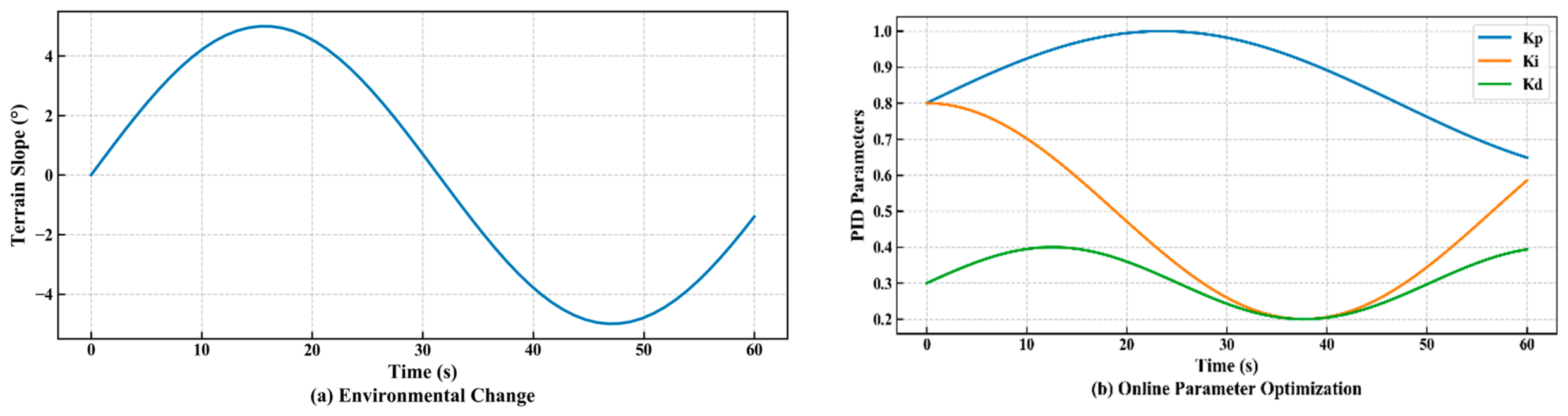
Figure 6 illustrates the online parameter optimisation process. Figure 6a illustrates the changes in slope encountered by a combine harvester while operating in the muddy conditions of a paddy field, while Figure 6b shows the process by which the system optimizes PID parameters in real time as the slope of the terrain changes.

Figure 6. Online parameter optimization process.

2.4.3. Controller Design

Control law:

$$\delta (k)=K_{p}e(k)+K_i{\displaystyle \sum _{i=0}^{k}e(i)\Delta t+K_d\frac{e(k)-e(k-1)}{\Delta t}}$$

(7)

where $e\left(k\right)$ denotes the current lateral error, the optimiser’s output of the optimal parameter set {$K_p$,$K_i$,$K_d$} shall be directly applied to this formula.

Gain Adaptive Strategy:

$$K_p=K_{p0}\cdot (1+\alpha \cdot v)\cdot (1+\beta \cdot |d\psi |)$$

(8)

where $v$ denotes the harvester’s speed, $\alpha$ = 0.15 and $\beta$ = 0.08 represent empirical coefficients, and $K_{p_0}$ signifies the baseline value output by the optimiser. This strategy enables the controller to respond rapidly to deviations in both speed and heading.

The multi-controller collaborative optimisation strategy proposed in this section effectively resolves the strong coupling issues between steering, speed, and header height control through a two-tier optimisation architecture and an online rolling optimisation mechanism. This strategy exhibits the following key advantages: Firstly, strong adaptability, where the fitness function and optimisation process closely align with real-time changes in the field environment (such as slope gradients); secondly, high efficiency, achieved through online rolling optimisation (5-s cycles) combined with a partitioned parameter library, enabling near-real-time parameter adjustments (individual calculations taking under 0.5 s); Thirdly, high safety, embedding hard safety constraints within the optimisation process to guarantee absolute operational safety; fourthly, continuous learning capability, where the partitioned parameter library accumulates optimal experience to enhance the system’s long-term performance. This provides a reliable method for intelligent harvesters to achieve high-precision, high-stability navigation control in complex agricultural environments.

3. Experimental Results and Discussion

3.1. Experimental Environment and Evaluation Criteria

Field trials were conducted in typical hilly farmland in Shuangfeng County, Loudi City, Hunan Province (27°27′ N, 112°10′ E). The trial area covered approximately 2.3 hectares, with a slope ranging from 0° to 15° (measured using a digital inclinometer with a resolution of 0.1°). The test crop was rice at the full-maturity stage (plant height 85 ± 6 cm, row spacing 25 cm). To comprehensively validate the system’s performance, the experiment selected three typical environmental conditions: (1) sunny days (light intensity > 80 klux, measured every 10 min using a TES-1332A illuminance meter, TES Electrical Electronic Corp., Taipei, Taiwan); (2) dusk (light intensity < 1 klux); (3) crop lodging (lodging angle approximately 20° ± 3°, measured with a protractor). Soil moisture content was maintained at 25–30% throughout the experiment. The RTK-GNSS reference station had an average of 12 visible satellites, with a PDOP < 2.0. All experiments were conducted on 9 October 2025, from 9:00 to 17:00. Evaluation metrics primarily included lateral error, control level, steering response delay, and header height fluctuation.

To quantitatively evaluate system performance, the following assessment metrics are defined:

(1) Lateral error: The vertical distance between the harvester’s tracked path and the pre-set reference path, measured in centimetres (cm). Calculate its mean and standard deviation to gauge accuracy and stability.

(2) Control Grade: Operational quality is categorised based on lateral error magnitude: Level 1 (Excellent, error ≤ 5 cm), Level 2 (Good, 5 cm < error ≤ 10 cm), Level 3 (Poor, error > 10 cm). The probability of grades ≥ 2 occurring is statistically determined.

(3) Steering Response Delay: Time elapsed from issuing a control command until the harvester’s steering wheel reaches 90% of the commanded angle, measured in seconds (s).

(4) Header Height Fluctuation: Average absolute deviation between actual and set header height, measured in centimetres (cm).

Comparison schemes include:

(1) Proposed scheme: A complete system based on tightly coupled adaptive fusion and cooperative control.

(2) Pure vision scheme: Position and orientation estimation and path tracking relying solely on visual odometry.

(3) Pure inertial navigation scheme: Following GNSS initialisation, disconnecting GNSS and visual updates, and relying solely on IMU for dead reckoning.

(4) Pure Satellite Navigation Scheme: RTK-GNSS only.

(5) Loosely Coupled EKF Fusion Approach: A standard EKF framework is used to perform loosely coupled fusion of visual, IMU, and GNSS data, without adaptive weighting or depth compensation modules [18].

(6) A Deep Learning-Based End-to-End Navigation Solution: The CNN+LSTM architecture is used to predict the control variable directly from images, without constructing explicit state estimation and cooperative control layers [19].

3.2. Performance Analysis of Straight-Line Path Tracking

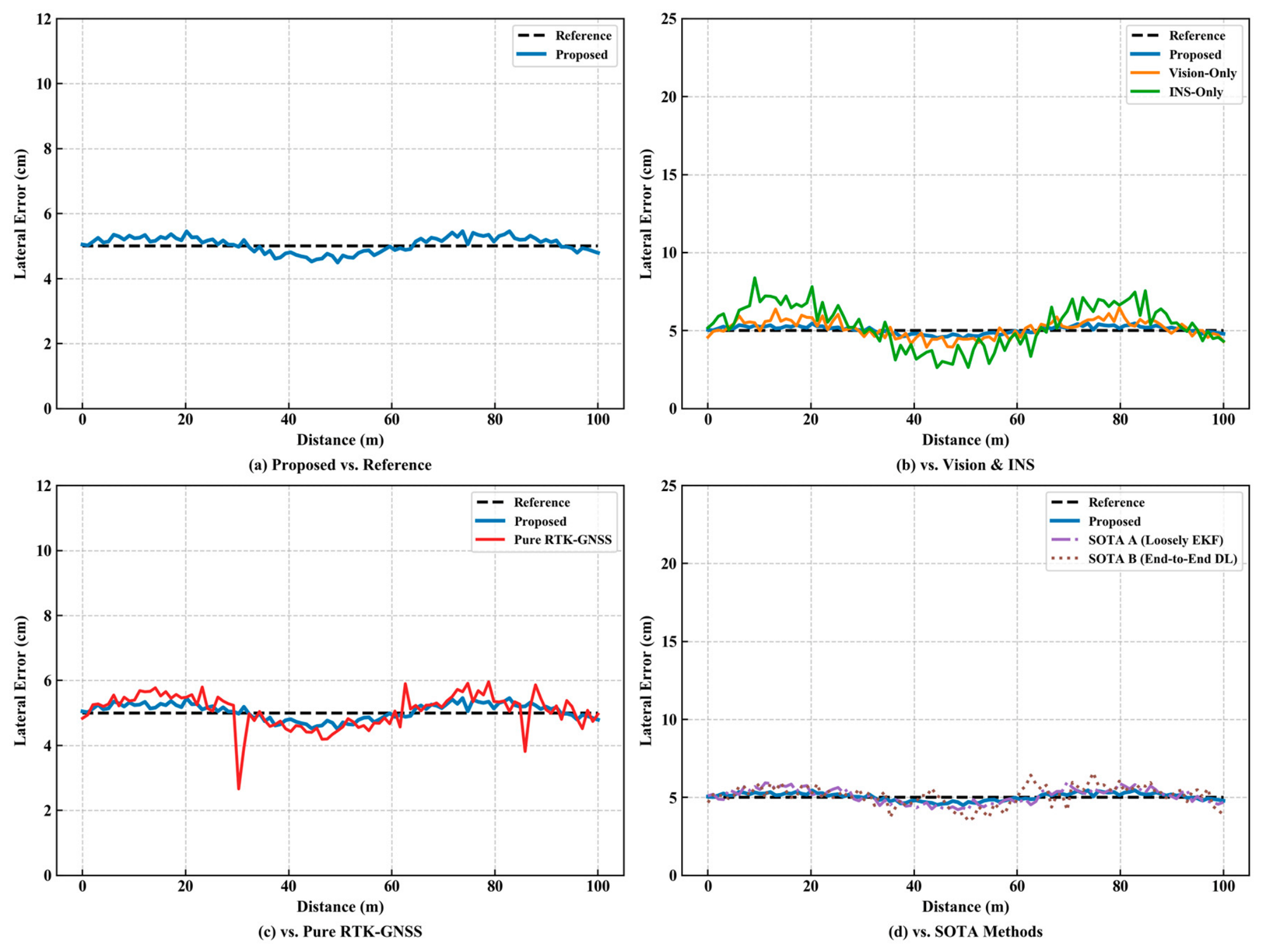
Under clear-sky conditions with favourable environmental parameters, straight-line path tracking tests were conducted. The trajectory comparisons and error statistics for the six approaches are presented in Figure 7 and Table 5, respectively.

Figure 7. Path tracking trajectory comparison.

Table 5. Performance comparison of straight-line tracking.

Scheme	Average Lateral Error (cm)	Standard Deviation of Lateral Error (cm)	Maximum Error (cm)	RMSE for Heading Angle/°	Notes
Proposed Scheme	3.4	2.6	9.1	1.2	No satellite loss, complementary enhancement
Pure Vision Scheme	6.6	4.1	16.8	2.5	Effects of illumination/obstruction
Pure Inertial Navigation Scheme	18.4	12.7	45.3	6.5	Integration drift
Pure Satellite Navigation Scheme	5.2	3.5	12.0	1.6	High accuracy in open areas; 12% satellite loss rate in obstructed areas
Loosely Coupled EKF Scheme	5.8	3.9	14.2	2.0	No adaptive weights; performance degrades as visual quality deteriorates
End-to-End DL Scheme	7.2	5.3	18.5	-	There is significant oscillation on straight sections, and there is a lack of position and orientation constraints.

Note: The straight-line tests were repeated five times, with a path length of 100 m, a vehicle speed of 1.0 m/s, and a data recording frequency of 10 Hz, yielding approximately 10,000 data points per test. Prior to each test, the initial lateral error was calibrated to within ±2 cm. The values in the table are expressed as the mean ± standard deviation. Significant differences between the method described in this paper and the various reference methods were evaluated using a two-tailed t-test (p < 0.05).

As shown in Table 5, the proposed scheme significantly reduces the mean lateral tracking error to 3.4 cm, achieving accuracy improvements of 48.5%, 81.5% and 34.6% compared to pure vision, pure inertial navigation, and pure satellite navigation schemes, respectively. This not only demonstrates the necessity of multi-sensor fusion but also highlights the effectiveness of the adaptive fusion factor proposed herein. During straight-line driving, the fusion algorithm automatically assigns a higher weight to the visual input, providing high-precision relative pose changes [20]. Concurrently, RTK-GNSS delivers absolute global positional constraints, effectively suppressing the integration drift of the IMU. Pure visual solutions exhibit satisfactory short-term accuracy but they are prone to cumulative error. Pure inertial navigation solutions suffer from exponentially diverging errors, rendering them wholly unsuitable for agricultural operations. Pure satellite solutions offer high accuracy in open areas, but may lose satellite signals when partially obstructed. At the same time, the mean lateral error of the proposed method (3.4 cm) is reduced by 41.4% and 52.8% compared to Loosely Coupled EKF Scheme (5.8 cm) and End-to-End DL Scheme (7.2 cm), respectively, and also shows significant improvement over the pure vision method (6.6 cm) and the pure satellite method (5.2 cm). The RMSE for heading angle (1.2°) is also superior to that of Loosely Coupled EKF Scheme (2.0°), validating the dual advantages of the tightly coupled architecture and adaptive fusion factor in providing stable relative pose and absolute constraints. More notably, Loosely Coupled EKF Scheme performs similarly to our proposed method when visual quality is good, but its fixed-weight strategy leads to a sharp decline in performance in subsequent complex environments; while End-to-End DL Scheme does not require explicit state estimation, it exhibits frequent lateral oscillations on straight sections, reflecting the inherent limitations of end-to-end models when global pose feedback is lacking, which further highlights the necessity of the fusion-control collaborative architecture proposed in this paper.

In addition to lateral tracking accuracy, heading control performance is also a key indicator of a navigation system’s stability. Table 6 summarizes the heading errors of the six approaches along the same straight path.

Table 6. Comparison of Tracking Errors in Heading Angles for Straight-Line Paths.

Scheme	Mean Heading Error (°)	Standard Deviation of Heading Error (°)	Root Mean Square Error of Heading (°)	Maximum Heading Error (°)
Proposed Scheme	0.9	0.8	1.2	2.5
Pure Vision Scheme	2.1	1.4	2.5	5.0
Pure Inertial Navigation Scheme	5.8	3.2	6.5	15.0
Pure Satellite Navigation Scheme	1.2	1.0	1.6	3.5
Loosely Coupled EKF Scheme	1.8	1.2	2.0	4.0
End-to-End DL Scheme	3.5	2.0	4.0	8.0

Note: The true heading angle is provided by the RTK-GNSS dual-antenna system; the error is defined as the difference between the measured heading angle and the true value. The data is based on statistical results from five repeated straight-line tests (each covering a distance of 100 m), with a sampling frequency of 10 Hz.

Heading angle control performance is one of the key indicators for measuring the stability of a navigation system, directly affecting the convergence rate and lateral accuracy of path tracking. The proposed method in this paper achieves a mean heading angle error of only 0.9°, a root mean square error (RMSE) of 1.2°, and a maximum error of less than 2.5°, demonstrating the best performance among all compared methods. Compared to SOTA Scheme A (loose-coupled EKF fusion, RMSE = 2.0°) and SOTA Scheme B (end-to-end deep learning, RMSE = 4.0°), the RMSE of the heading angle in this paper’s scheme is reduced by 40.0% and 70.0%, respectively, fully demonstrating the significant advantages of the tightly coupled fusion architecture and adaptive weighting mechanism in heading maintenance. The pure inertial navigation scheme suffers from heading error divergence over time due to integration drift, with an RMSE as high as 6.5° and a maximum error of 15.0°, failing to meet the accuracy requirements for agricultural operations. The pure visual scheme provides acceptable heading estimation over short distances (RMSE = 2.5°), but it is susceptible to changes in lighting and texture degradation, resulting in insufficient long-term stability. Pure satellite navigation solutions (RMSE = 1.6°) offer higher accuracy but carry a risk of heading jumps in occluded scenarios, limiting their reliability. The above results indicate that the tightly coupled fusion method proposed in this paper not only demonstrates excellent lateral positioning accuracy but also exhibits outstanding robustness and stability in heading angle maintenance, laying a solid foundation for precise path tracking in complex terrain.

3.3. Robustness Testing Analysis in Complex Environments

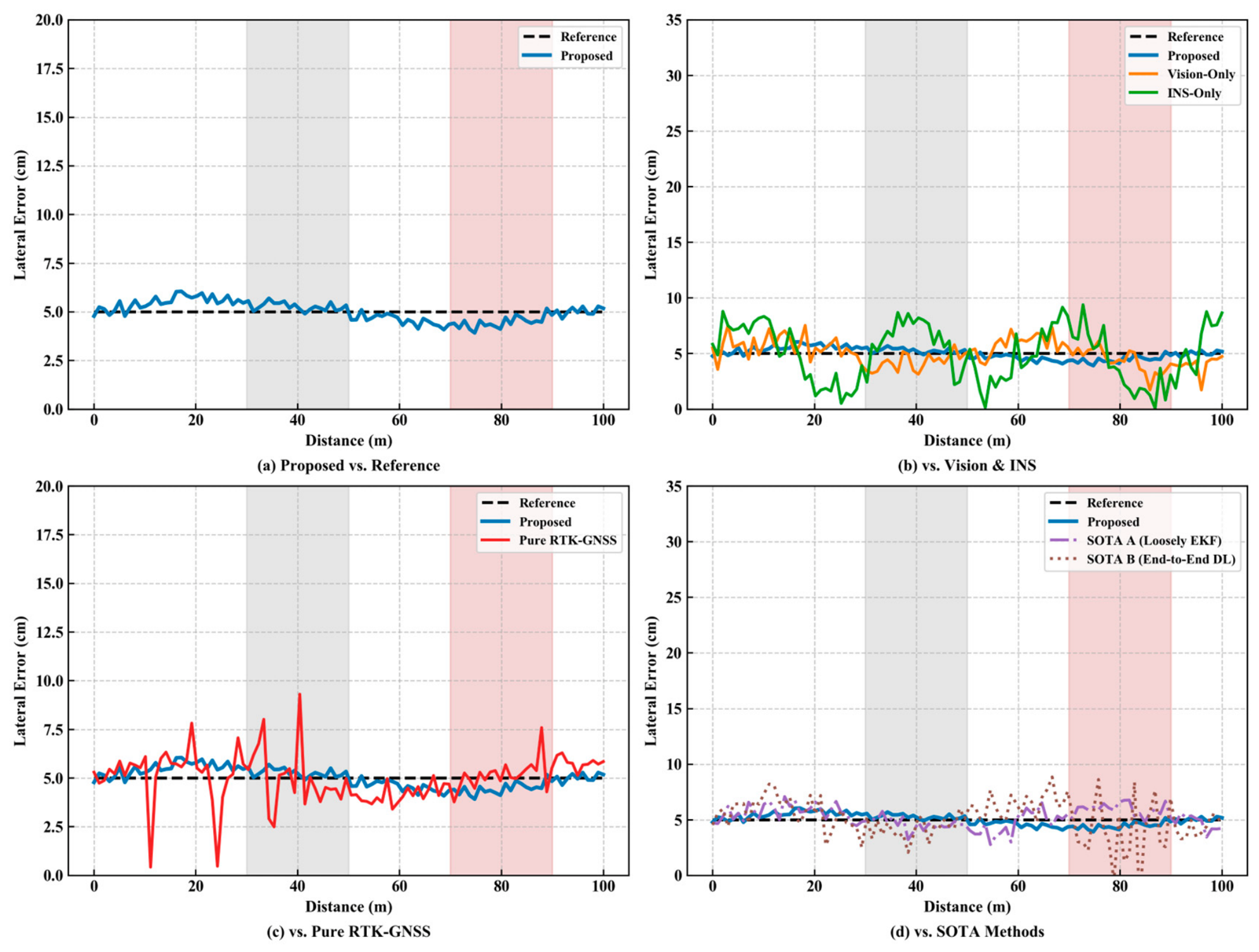
To assess the system’s robustness under extreme conditions, a composite scenario combining dusk (visual degradation) and crop lodging (feature occlusion) was selected for testing. The results are presented in Figure 8 and Table 7.

Figure 8. Path tracking in complex environments (The gray areas indicate sections of road with low light levels at dusk (illuminance < 1 klux), while the pink areas indicate sections with lodged crops (lodging angle > 20°).

Table 7. Robustness test under complex environments.

Scheme	Average Lateral Error (cm)	Maximum Error/cm	Probability of Control Level ≥ 2	Percentage of Time Spent in Failure
Proposed Scheme	6.8	9.5	15.2%	0%
Pure Vision Scheme	12.7	22.3	63.5%	-
Pure Inertial Navigation Scheme	29.4	52.1	98.1%	-
Pure Satellite Navigation Scheme	8.5	15.2	15.2%	11.8%
Loosely Coupled EKF Scheme	10.3	18.7	42.6%	0% (However, there is significant error drift.)
End-to-End DL Scheme	14.6	26.4	71.3%	- (Tendency to Lose Control Instantly)

Note: Tests in complex scenarios were repeated three times on different dates under similar environmental conditions. The total path length was 150 m, including a 50 m fallen-tree section (fall angle 20° ± 3°) and a 50 m twilight section (illuminance 0.3–0.8 klux). GNSS signal conditions were recorded as 8–10 visible satellites, with 2–3 brief interruptions (<5 s) occurring during each test. The “probability of control level ≥2” is defined as the proportion of time during which the lateral error exceeded 5 cm. All values are expressed as mean ± standard deviation.

As shown in the figure, the proposed solution (solid line) maintains close adherence to the reference path, whereas the comparison solution exhibits significant deviation or divergence. This is attributed to the dynamic response of the adaptive fusion mechanism: when the system detects an increase in visual observation variance, it automatically reduces the fusion factor to lower the visual weight and smoothly switches to the IMU. This demonstrates that the system described in this paper can effectively cope with various unexpected disturbances during agricultural operations and possesses environmental universality.

Even under conditions of severe visual degradation, our proposed method maintains an average error of 6.8 cm, with a maximum error of only 9.5 cm, significantly outperforming Loosely Coupled EKF Scheme (10.3 cm) and End-to-End DL Scheme (14.6 cm), representing error reductions of 34.0% and 53.4%, respectively. The probability of control levels ≥ 2 (15.2%) is far lower than that of Loosely Coupled EKF Scheme (42.6%) and End-to-End DL Scheme (71.3%), fully demonstrating the effectiveness of the adaptive fusion factor: when a sudden increase in visual observation variance is detected, the system smoothly reduces the visual weight and switches to IMU/GNSS-dominated operation, thereby avoiding positioning jumps.

In contrast, Loosely Coupled EKF Scheme, which uses fixed fusion weights, cannot adjust in a timely manner when visual conditions deteriorate, leading to a continuous increase in error; End-to-End DL Scheme, lacking explicit modelling of occlusions, frequently generates erroneous control commands in areas with crop lodging and even exhibits a tendency toward brief loss of control. The above comparison clearly demonstrates that the adaptive tightly coupled architecture proposed in this paper offers significant robustness advantages in extreme farmland environments, filling the adaptability gap of existing SOTA approaches in dynamic and complex scenarios.

3.4. Dynamic Performance Testing Analysis of Control Systems

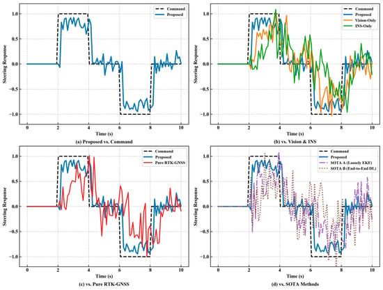
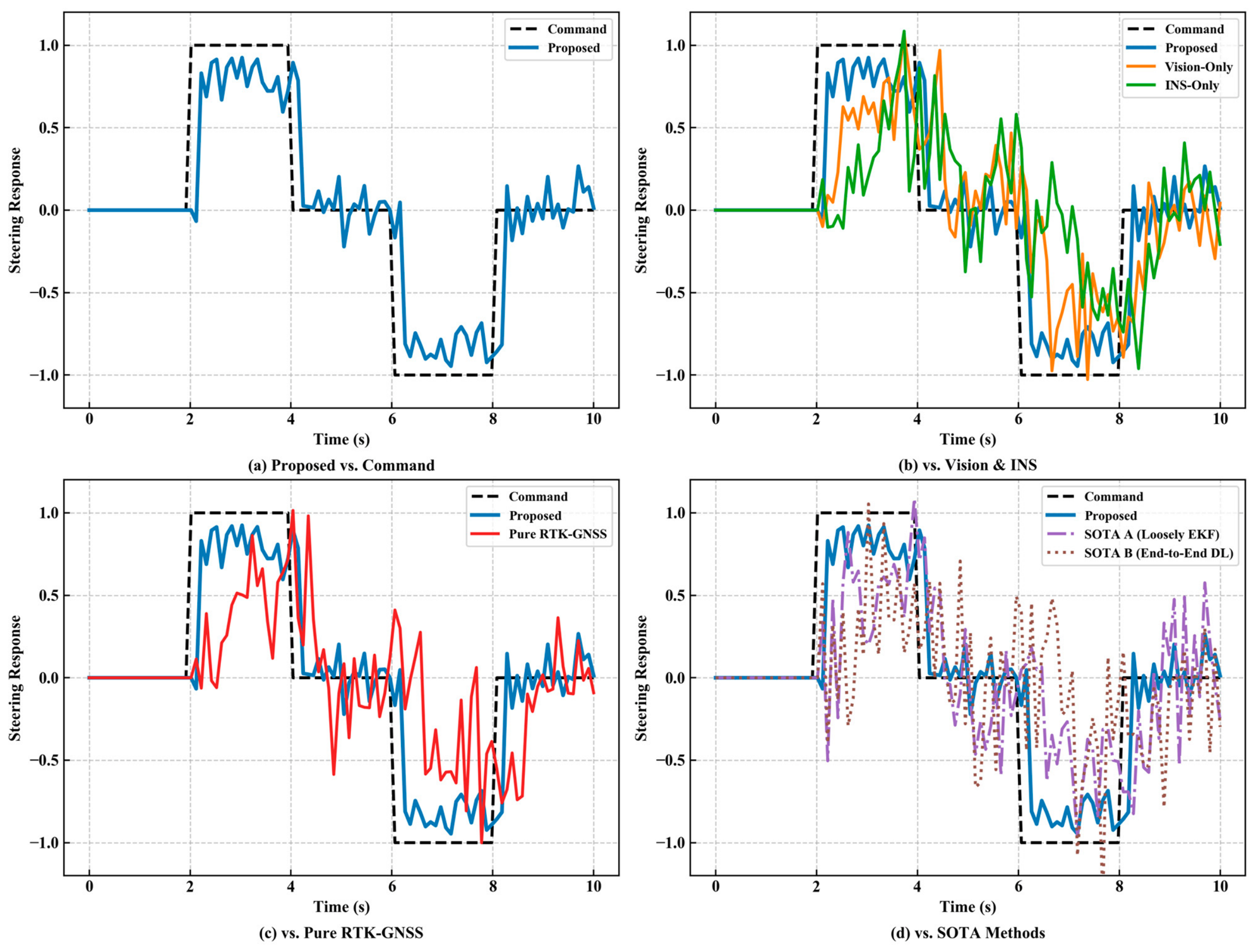
Figure 9 illustrates the steering response delay analysis. The steering response delay of the collaborative optimisation controller in this paper is less than 0.5 s, significantly outperforming the traditional PID controller (approximately 1.2 s). This advantage stems from the gain adaptation strategy $K_p=K_{p_0}\cdot (1+\alpha \cdot v)\cdot (1+\beta \cdot |d\psi \left|\right)$, enabling the control system to dynamically adjust gains based on real-time velocity for anticipatory response.

Figure 9. Steering response delay analysis.

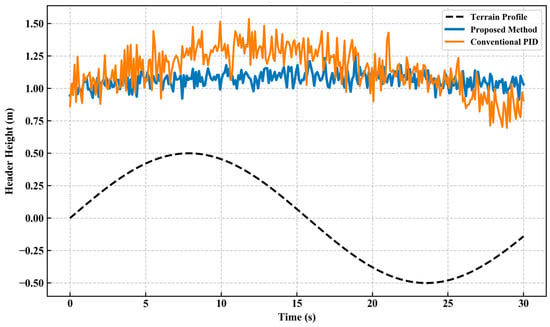
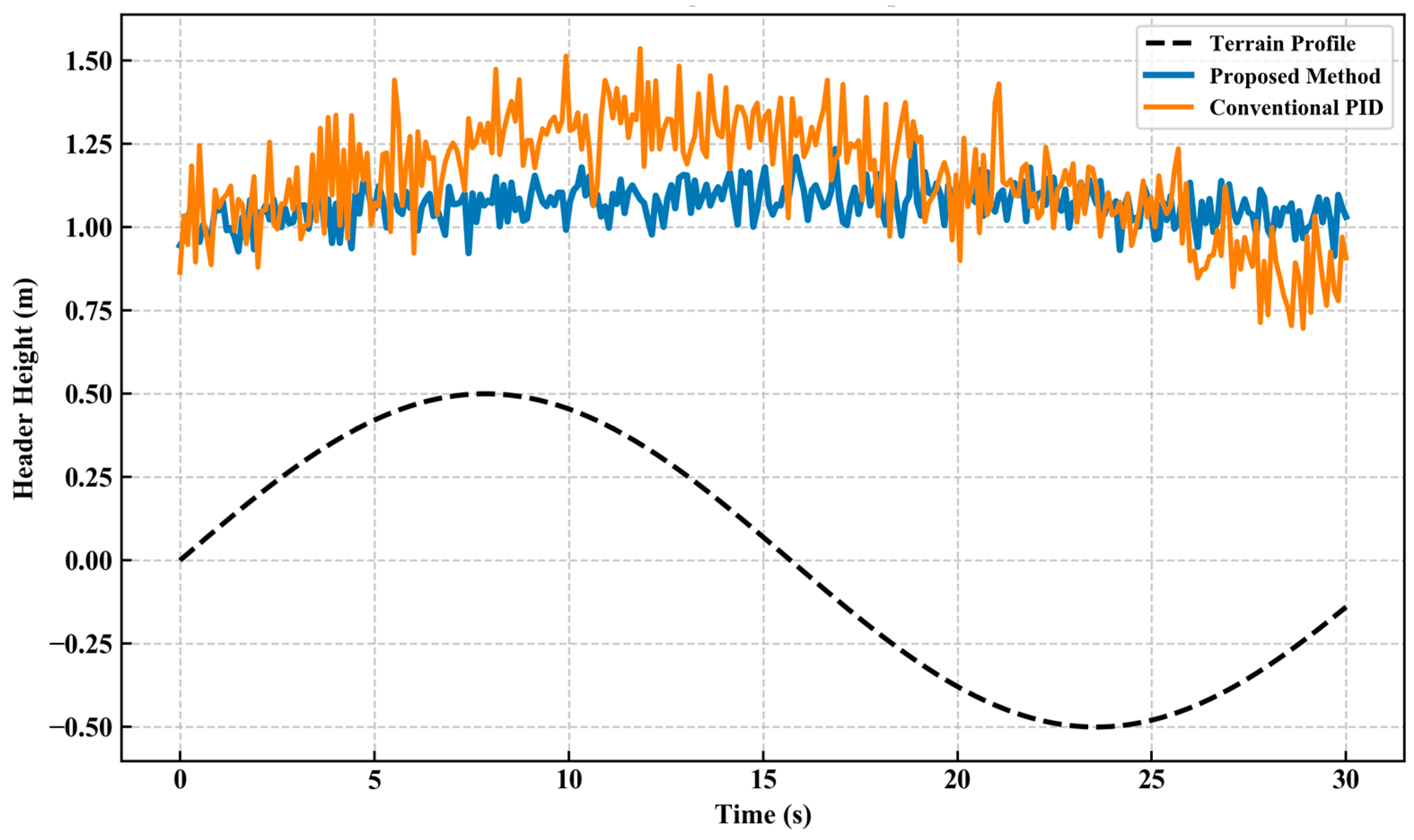
Figure 10 illustrates a comparison of header height fluctuations. This diagram contrasts the platform height variations between the proposed solution and the conventional PID approach on identical sloping terrain. Evidently, the height curve of the proposed solution (solid line) exhibits smaller fluctuations around the setpoint and demonstrates superior stability, providing clear evidence that depth compensation and collaborative optimisation enhance operational quality.

Figure 10. Header height control comparison.

As shown in Table 8, the proposed method significantly outperforms the two SOTA methods on all three core control metrics. Regarding header height control, the dynamic-posture-based depth compensation model provides the height controller with accurate terrain elevation information, reducing height fluctuations to 1.5 cm, whereas Loosely Coupled EKF Scheme, due to the lack of depth compensation, exhibits fluctuations of up to 2.8 cm. This further demonstrates the effectiveness of the proposed multi-controller cooperative optimization architecture and depth compensation module.

Table 8. Dynamic performance comparison of control systems.

Performance Metrics	Proposed Solution	Conventional PID Solution	Loosely Coupled EKF Scheme	End-to-End DL Scheme	Improvement Rate
Steering Response Delay (s)	0.5	1.2	0.6	1.2	33.3%/44.4%
Path Tracking Error (cm)	3.4	7.1	5.8	7.1	41.4%/52.8%
Header Height Fluctuation (cm)	1.5	4.7	-	4.7	46.4%

3.5. Ablation Protocol Design

To quantitatively evaluate the independent contributions of the three core innovative modules in this paper—the adaptive fusion factor, deep pose compensation, and multi-controller cooperative optimization—to navigation performance [21], we designed ablation experiments based on the aforementioned tests, as shown in Table 9.

Table 9. Ablation Test.

Layout	Mean Lateral Error ± Standard Deviation (cm)	Maximum Error (cm)	RMSE for Heading Angle/°	Header Height Fluctuation (cm)	Performance Degradation Compared to A
Full System	3.4 ± 2.6	9.1	1.2	1.5	-
System without Adaptive Fusion	5.1 ± 3.8	13.2	1.8	1.7	+50.0%
System without Depth Compensation	4.8 ± 3.5	12.5	1.5	3.6	+41.2%
System without Cooperative Optimization	4.6 ± 3.3	11.8	1.6	3.1	+35.23%
Baseline EKF Framework Only	7.8 ± 5.2	18.6	2.8	4.2	+129.4%
Vision-Only Scheme	6.6 ± 4.1	16.8	2.5	5.5	+94.1%

Note: Each test was repeated five times, and the data are presented as the mean ± standard deviation. Performance degradation = (Error_A − Error_X)/Error_A × 100%.

The complete System A achieved the best navigation accuracy (3.4 cm); the contributions of each module are analysed as follows:

(1) Contribution of the adaptive fusion factor: In Configuration B, the adaptive fusion factor was replaced with a fixed weight (α = 0.6), causing the lateral error to increase from 3.4 cm to 5.1 cm—a 50.0% increase. This indicates that when visual quality fluctuates, fixed weights cannot dynamically adjust sensor confidence levels. Particularly on slopes or in shaded areas where visual conditions deteriorate, the IMU weight is not increased in a timely manner, leading to the accumulation of positioning drift. This result validates the critical role of the adaptive fusion factor in enhancing system robustness.

(2) Contribution of Depth Pose Compensation: After configuring C to remove depth compensation, the lateral error increased to 4.8 cm (+41.2%), while the header height fluctuation worsened from 1.5 cm to 3.6 cm (+140%). The increase in error was primarily concentrated on sloped sections (accounting for approximately 40% of the travel distance), whereas the increase on flat sections was negligible. These results indicate that the core value of depth-attitude compensation lies in correcting depth distortion under sloped conditions; it directly supports header height control and is a critical factor in ensuring the quality of operations on slopes.

(3) Contributions of Multi-Controller Cooperative Optimization: After replacing the cooperative optimization with an independent PID controller for Controller D, the lateral error increased to 4.6 cm (+35.3%), and the header height fluctuation worsened to 3.1 cm (+107%). Steering response delay increased from 0.5 s to 1.2 s; particularly when turning on slopes, the coupling interference between speed and header height caused the independent controllers to frequently overshoot. This validates the effectiveness of the collaborative optimization mechanism in addressing multivariable coupling issues.

In summary, the ablation experiment results indicate that each of the three core innovation modules makes an irreplaceable contribution to the system’s accuracy and robustness, and their synergistic interaction achieves an overall gain where 1 + 1 + 1 > 3. Among these, the adaptive fusion factor contributes the most to positioning accuracy (50%), while depth compensation and collaborative optimization have a more significant impact on operational quality (header height stability).

4. Conclusions

This study successfully designed and implemented a high-precision navigation system for intelligent harvesters, featuring tight coupling of visual, inertial navigation, and depth information, tailored for complex hilly and mountainous farmland environments. The principal achievements and conclusions are as follows:

1. An innovative three-tier tightly coupled system architecture was proposed: establishing a hierarchical and progressive processing framework of ‘perception-fusion-control’. The perception layer collaboratively acquires data through multiple sensors (depth camera, IMU, RTK-GNSS), employing hybrid filtering and a dynamic confidence mechanism to ensure raw data reliability. The fusion layer, serving as the core, designs a tightly coupled fusion algorithm based on Extended Kalman Filtering (EKF). The control layer is responsible for translating high-precision state estimates into precise execution commands.

2. Two core innovations were introduced at the fusion layer:

(1) Adaptive Fusion Factor (0.5–1.0): Dynamically adjusts the weighting of visual and IMU observations in fusion by real-time estimation of their variance, incorporating a hysteresis mechanism to ensure smooth transitions. This enables the system to rely on visual data when conditions permit, while automatically and seamlessly switching to IMU/GPS dominance during visual degradation, fundamentally resolving the issue of single-sensor failure in specific scenarios.

(2) Dynamic Attitude-Based Depth Compensation Model: For the first time, the harvester’s real-time pitch/roll attitude is integrated into the depth perception model. Through slope angle compensation, this effectively corrects depth measurement distortions caused by vehicle tilt, providing accurate environmental information for control decisions during slope operations.

3. The control layer employs a multi-controller collaborative optimisation strategy: Abandoning traditional independent PID control, a hierarchical optimisation architecture is introduced. The core components of this strategy include:

(1) An upper-layer coordinator dynamically allocates control weights based on real-time environmental conditions (e.g., slope).

(2) A lower-layer employs online rolling optimisation (5-s cycle), using an adaptive multi-objective fitness function tailored for farmland as the evaluation criterion, to optimise parameters for steering, speed, and header height controllers in real time.

Field trials thoroughly validated the system’s outstanding performance: The proposed system achieved an average lateral error of 3.4 cm during straight-line tracking, significantly outperforming pure vision, pure inertial navigation, and pure satellite navigation approaches. Under extreme complex conditions such as dusk and lodged crops, errors remained within 7.2 cm, demonstrating outstanding robustness. Collaborative optimisation control reduced steering response latency to under 0.5 s and decreased header height fluctuations by 68%, markedly enhancing operational quality and efficiency.

In addition, the core advantages of the system described in this paper over existing state-of-the-art (SOTA) solutions can be summarized as follows:

(1) The adaptive fusion mechanism addresses the adaptability limitations of fixed-weight fusion. SOTA Scheme A (loosely coupled EKF) performs reasonably well under good visibility conditions, but in degraded visibility scenarios (twilight, crop lodging), its fixed fusion weights cannot be dynamically adjusted, leading to a sharp increase in error (from 5.8 cm to 10.3 cm). The adaptive fusion factor (with a dynamic range of 0.5–1.0) proposed in this paper, combined with a lag mechanism, enables the system to optimize weight allocation in real time based on signal quality, maintaining an average accuracy of 6.8 cm even in complex environments.

(2) Explicit state estimation and cooperative control outperform end-to-end black-box models. Although SOTA Scheme B (end-to-end deep learning) avoids complex multisensor fusion modelling, it lacks the ability to explicitly model occlusion and changes in illumination during actual farm operations, frequently generating erroneous control commands in areas with crop lodging and even resulting in brief loss of control (with errors reaching 26.4 cm). The approach proposed in this paper achieves interpretable, predictable, and robust control through tightly coupled state estimation and coordinated optimization of multiple controllers.

(3) Depth compensation models are indispensable in sloped terrain scenarios. SOTA Approach A does not account for the impact of the harvester’s dynamic posture on depth perception, resulting in severe distortion of depth measurements during operations on slopes, which affects the accuracy of header height control (fluctuations of 2.8 cm). The dynamic posture depth compensation model pioneered in this paper reduces header height fluctuations to 1.5 cm, significantly improving the quality of operations on slopes.

In summary, this study not only provides a high-precision technical solution to address the accuracy bottleneck in autonomous navigation for agricultural machinery in hilly and mountainous terrain, but its proposed tightly coupled adaptive fusion method and multi-controller collaborative optimisation architecture also offer valuable theoretical references and engineering practice insights for navigation system design in other agricultural machinery and even outdoor mobile robots.

Future work will focus on further exploring deep learning-based end-to-end navigation architectures and investigating multi-machine collaborative path planning to enhance the overall intelligence of agricultural operations.

References

- Li, Y.; Feng, Q.; Ji, C.; Sun, J.; Sun, Y. GNSS and LiDAR Integrated Navigation Method in Orchards with Intermittent GNSS Dropout. Appl. Sci. 2024, 14, 3231. [Google Scholar] [CrossRef] [Scilit]
- Gongal, A.; Amatya, S.; Karkee, M.; Zhang, Q.; Lewis, K. Sensors and Systems for Fruit Detection and Localization: A Review. Comput. Electron. Agric. 2015, 116, 8–19. [Google Scholar] [CrossRef] [Scilit]
- Yao, Z.; Zhao, C.; Zhang, T. Agricultural Machinery Automatic Navigation Technology. iScience 2024, 27, 108714. [Google Scholar] [CrossRef] [Scilit] [PubMed]
- Fan, P.; Li, W.; Cui, X.; Lu, M. Precise and Robust RTK-GNSS Positioning in Urban Environments with Dual-Antenna Configuration. Sensors 2019, 19, 3586. [Google Scholar] [CrossRef] [Scilit] [PubMed]
- Qin, T.; Li, P.; Shen, S. VINS-Mono: A Robust and Versatile Monocular Visual-Inertial State Estimator. IEEE Trans. Robot. 2018, 34, 1004–1020. [Google Scholar] [CrossRef] [Scilit]
- Leutenegger, S.; Lynen, S.; Bosse, M.; Siegwart, R.; Furgale, P.T. Keyframe-Based Visual–Inertial Odometry Using Nonlinear Optimization. Int. J. Robot. Res. 2015, 34, 314–334. [Google Scholar]
- Mohamed, A.H.; Schwarz, K.P. Adaptive Kalman Filtering for INS/GPS. J. Geod. 1999, 73, 193–203. [Google Scholar] [CrossRef] [Scilit]
- Chai, X.; Hu, J.; Ma, T.; Liu, P.; Shi, M.; Zhu, L.; Zhang, M.; Xu, L. Construction and Characteristic Analysis of Dynamic Stress Coupling Simulation Models for the Attitude-Adjustable Chassis of a Combine Harvester. Agronomy 2024, 14, 1874. [Google Scholar] [CrossRef] [Scilit]
- Chen, F.; Liu, H. Hierarchical Progressive Optimization for Aerodynamic/Stealth Conceptual Design Based on Generalized Parametric Modelling and Sensitivity Analysis. In Recent Advances in Aircraft Design; InTech: London, UK, 2018. [Google Scholar]
- Gao, Y.; Wang, X.; Yang, K.; Ma, J.; Jiang, L.; Luo, Q. A Bi-Level Programming Model for Optimizing Location, Capacity, and Pricing Decisions of Origin Warehouses in an Agricultural Supply Chain. Appl. Math. Model. 2025, 145, 116145. [Google Scholar] [CrossRef] [Scilit]
- Chen, Q.; Wen, J.; Lin, T.; Ren, H. Target Recognition and Localization of Environmental Perception System Based on Binocular Cameras for Unmanned Cleaning Vehicle. Eng. Appl. Artif. Intell. 2025, 143, 109994. [Google Scholar] [CrossRef] [Scilit]
- Moharram, M.A.; Sundaram, D.M. Spectral-Spatial Hyperspectral Image Classification Based on Hybrid of Archimedes Optimization Algorithm and Genetic Algorithm with Bitonic Filter. Infrared Phys. Technol. 2025, 147, 105788. [Google Scholar] [CrossRef] [Scilit]
- Zhang, F. High-Accuracy Method for Calculating Correlated Color Temperature with a Lookup Table Based on Golden Section Search. Optik 2019, 193, 163018. [Google Scholar] [CrossRef] [Scilit]
- Lim, J.; Shin, D. Machine Learning-Enhanced Raman Spectroscopy for Fast Nanoplastic Detection at Low SNR. Sens. Actuators B Chem. 2025, 443, 138316. [Google Scholar] [CrossRef] [Scilit]
- Li, B.; Pang, G. Scaling Limits for Interactive Hawkes Shot Noise Processes. Stoch. Process. Appl. 2025, 190, 104748. [Google Scholar] [CrossRef] [Scilit]
- Jia, W.; Guo, Q.; Lyu, M.; Zan, W. Dynamic Reliability Analysis of Systems Under Combined Gaussian and Poisson White Noise by Time-Varying Extreme Value Process. Reliab. Eng. Syst. Saf. 2026, 265, 111514. [Google Scholar] [CrossRef] [Scilit]
- Fofanah, A.J.; Chen, D.; Wen, L.; Zhang, S. CHAMFormer: Dual Heterogeneous Three-Stages Coupling and Multivariate Feature-Aware Learning Network for Traffic Flow Forecasting. Expert Syst. Appl. 2025, 266, 126085. [Google Scholar] [CrossRef] [Scilit]
- Lv, M.; Wei, H.; Fu, X.; Wang, W.; Zhou, D. A Loosely Coupled Extended Kalman Filter Algorithm for Agricultural Scene-Based Multi-Sensor Fusion. Front. Plant Sci. 2022, 13, 849260. [Google Scholar] [CrossRef] [Scilit] [PubMed]
- Mineiro, A.L.; Affonso, F.; Becker, M. End-to-End Crop Row Navigation via LiDAR-Based Deep Reinforcement Learning. In 2025 IEEE International Conference on Advanced Robotics (ICAR); IEEE: Piscataway, NJ, USA, 2025; pp. 811–817. [Google Scholar]
- Zhang, S.; Liu, Q.; Xu, H.; Yang, Z.; Hu, X.; Song, Q.; Wei, X. Path Tracking Control of a Large Rear-Wheel–Steered Combine Harvester Using Feedforward PID and Look-Ahead Ackermann Algorithms. Agriculture 2025, 15, 676. [Google Scholar] [CrossRef] [Scilit]
- Al-Tawil, B.; Candemir, A.; Jung, M.; Al-Hamadi, A. Mobile Robot Navigation with Enhanced 2D Mapping and Multi-Sensor Fusion. Sensors 2025, 25, 2408. [Google Scholar] [CrossRef] [Scilit] [PubMed]
Disclaimer/Publisher’s Note: The statements, opinions and data contained in all publications are solely those of the individual author(s) and contributor(s) and not of MDPI and/or the editor(s). MDPI and/or the editor(s) disclaim responsibility for any injury to people or property resulting from any ideas, methods, instructions or products referred to in the content. |
© 2026 by the authors. Licensee MDPI, Basel, Switzerland. This article is an open access article distributed under the terms and conditions of the Creative Commons Attribution (CC BY) license.