Improved MobileNetV2 Architecture with Modified Lite Attention Model for Detection of Plant Leaf Disease

Abstract

Global agriculture is seriously threatened by plant diseases, which result in large losses in both productivity and quality. Timely and accurate disease detection is essential for effective crop management and food security. This work presents an improved MobileNetV2 architecture with Modified Lite Attention (MLA) Model for detecting plant leaf disease. Our methodology incorporates pre-processing, feature extraction through attention model, convolution layers, and classifying into diseased or healthy categories. Further, multiclassification of diseases is performed on a dataset comprising 4432 samples including whitefly, leaf spot, leaf curl, yellowish and healthy leaves. The proposed attention model is compared with existing attention models like CBAM (Convolutional Block Attention Model), SE (Squeeze and Excitation), ECA (Efficient Channel Attention) and SDMnet (Spatially Dilated Multi-Scale Network) to validate our hybrid MLA feature extraction technique. Customizing the categorization with fully connected layers and utilisation of a pre-trained MobileNetV2 model allow the system to achieve excellent results. Findings show encouraging accuracy, surpassing 97% compared to existing techniques for multiclass dataset classification. The integration of MobileNetV2 with custom dense layers enables robust detection even with limited datasets, making it ideal for use in mobile or low-resource agricultural environments. Further, the proposed method is tested on the PlantVillage dataset consisting of 10,836 samples using K-Fold cross-validation for K = 5 and K = 4 to obtain an average accuracy of 98.4% and 98.69%, respectively.

1. Introduction

Crop diseases continue to be a significant obstacle in agricultural growth, market standards, and farmer earnings globally. These diseases, usually triggered by bacteria, fungi, or viruses, generally present as visible signs on plant leaves. Timely and precise detection of leaf diseases is essential for sustainable agriculture, food security, and enhanced livelihoods for farmers. Due to swift progress in artificial intelligence (AI) and computer vision, smart crop monitoring systems have developed into efficient resources for disease control and precision farming [1,2]. The investigation into plant disease identification can be classified into two main types: traditional feature-based methods and deep learning-based strategies. Conventional techniques consist of obtaining manually designed features such as hue, pattern, and form, followed by categorization with models like support vector machines (SVMs), artificial neural networks (ANNs), or k-nearest neighbours (KNNs). For instance, segmentation along with histogram of oriented gradients (HOG) and SVM have been utilized for recognizing leaf lesions [3]. Likewise, frameworks for feature selection combined with SVM and ANN have also been assessed [4]. Although these techniques are simple and easy to understand, they are very susceptible to changes in lighting, obstructions, and intricate backgrounds, which hinders their effectiveness in real-world situations [5].

Deep learning has greatly enhanced the classification of plant diseases, as convolutional neural networks (CNNs) demonstrate better generalization than conventional methods for crops such as maize, tomato, and mango [6,7]. Transfer learning, in which pre-trained models are modified for agricultural datasets, has improved performance even with limited data availability [8,9,10]. Hybrid networks that integrate attention or multi-scale features have shown enhanced robustness in capturing local lesion specifics and the broader context of leaves [11]. Nevertheless, CNNs generally demand significant computational power, limiting their applicability in mobile or edge environments. Numerous studies have indicated positive findings. A model based on EfficientNet-B4 attained impressive classification accuracy [12], whereas lightweight architectures like SqueezeNet [13] have been explored for their stability and effectiveness with small and imbalanced datasets. These studies emphasize the possibilities of deep learning for detecting chili diseases but also expose ongoing problems, such as overfitting, inadequate results in real-field scenarios, and an absence of systematic ablation analyses. Research has suggested real-time monitoring systems that integrate CNN-based classification with mobile or web platforms to assist farmers [14]. Collaborative training methods utilizing federated learning have been studied to maintain data privacy [15]. Despite the potential of these frameworks, many remain confined to controlled settings and lack extensive validation in real-world scenarios. In conclusion, traditional techniques provide clarity but struggle in changing environmental conditions. Deep learning and transfer learning methods enhance robustness, but significant challenges persist, such as inadequate datasets, imbalance issues, significant inter-class similarity in field images, and challenges in deployment within resource-limited settings. This study suggests a method for categorizing diseases of chili leaves that combines robust preprocessing, transfer learning using modified MobileNet architecture and effective deep learning.

The main contributions of this work are summarized as follows:

• A compact yet robust classification framework is proposed by utilizing MobileNetV2 as the base model, integrated with a Modified Lite Attention (MLA) mechanism and enhanced using dropout-regularized fully connected layers.
• The proposed attention model is systematically compared with existing attention mechanisms, including CBAM (Convolutional Block Attention Module), SE (Squeeze and Excitation), ECA (Efficient Channel Attention), and SDMNet (Spatially Dilated Multi-Scale Network), to validate the effectiveness of the hybrid MLA-based feature extraction technique.
• A modified transfer learning approach is developed to extract more discriminative and accurate features from chilli plant leaf images.
• The proposed method is evaluated against prominent existing architectures such as SqueezeNet, ShuffleNet, EfficientNet, Xception, and the baseline MobileNetV2, using the same dataset for fair comparison.
• The proposed framework achieves an optimal balance between computational efficiency and classification accuracy by employing a lightweight architecture with validated performance metrics.

The remaining portions of the paper are arranged as follows: Section 2 presents background information on the topics covered in this study and then dives into a survey of similar works. Section 3 presents an overview of the suggested approach along with the steps involved in diagnosing a chilli plant’s disease. Section 4 provides an account of the experimental design and results analysis. As the report draws to an end, the conclusion points out its shortcomings and makes recommendations for more study.

2. Related Works

The study [16] introduces a multi-scale convolutional module designed to capture disease features at varying spatial resolutions, enabling the model to extract both fine-grained and rough texture patterns in chili leaf images. While this approach enhances feature richness, the method lacks any form of attention mechanism, resulting in limited ability to prioritize disease-related regions over background noise or healthy tissue. Moreover, the multi-scale architecture increases computational complexity, making the model comparatively heavier and unsuitable for mobile or edge deployment. The absence of attention-based regularization also makes the network more likely to overfit when trained on small agricultural datasets and its generalization under variable lighting conditions or subtle disease stages remains strained.

The study [17] proposes an attention-enhanced MobileNetV2 backbone with the aim of improving feature extraction for plant disease classification. An attention mechanism further enhances the network’s ability to pay attention to some image parts of interest, thus delivering improved performance compared to the original MobileNetV2. However, the model only uses a one-level attention mechanism and thus is unable to refine features in various stages of the network. The shallow placement of this attention limits the effectiveness of the model in capturing subtle variations in the diseases, particularly in fine-grained multi-class problems. Besides this, the proposed approach fails to satisfactorily prevent overfitting when the agricultural dataset is small, and generalization capabilities are somewhat poor under various lighting and background conditions. Having only one attention block, combined with modest improvements in robustness, points to more comprehensive feature refinement being necessary for consistently high real-world performance.

The article [18] proposes a hybrid architecture, combining two deep backbone networks with an attention layer, to improve feature representation for chili leaf disease classification. While combining VGG16 and EfficientNetB0 gives the model rich hierarchical features, its heavy structure suffers from high parameters and increased training and inference complexities. Such significant architectural overhead greatly reduces its suitability for real-time or mobile deployment, which is often highly desired in agricultural applications. Furthermore, the deep structure of this hybrid network increases the overfitting risk of relatively small-scale plant disease datasets, despite the existence of attention mechanisms in the model architecture. Again, such dependency on large computational resources and limited adaptability in low-resource environments point out inherent constraints on scalability and practical field usage.

This study [19] presents an architecture based on MobileNet, optimized for fast inference in guava leaf disease detection. Its lightweight nature makes it suitable for real-time applications, especially on resource-constrained devices. However, the model solely depends on the basic feature extraction from MobileNet without incorporating attention or higher-order refinement mechanisms. Therefore, it cannot capture subtle and fine-grained disease patterns. Due to this, the performance of this model degrades when applied in a multi-class scenario where differentiating between visually similar leaf conditions is crucial. Moreover, without deeper feature enhancement, the robustness of the network is restricted under variations in lighting conditions, leaf orientation, and background clutter. While fast, the relatively shallow feature discriminative capability represents limitations in accuracy and generalization for more challenging disease classification tasks.

Lu et al. [20] propose a lightweight crop disease identification model with an improved MobileNetV2 architecture. In this approach, they integrate the RepMLP module to enhance global feature perception and incorporate ECA for emphasizing disease-relevant channels. The model still maintains low computational cost by using depth-wise separable convolutions and Hardswish activation, achieving a good accuracy–efficiency trade-off. Although this approach improves global feature extraction and reduces the model size to 0.91 M parameters, it still has some key limitations. The model has a predisposition towards capturing channel-wise attention, without spatial attention or edge-aware feature refinement, limiting its capacity to correctly segment disease lesions from complex, real-world backgrounds. At the same time, RepMLP enhances global sensing but does not explicitly model morphological or texture-level Edge Priors essential for early-stage disease detection. In addition, the heavy reliance on the Plant Village dataset, while captured in controlled settings, limits the generalization under real agricultural conditions caused by variable lighting, occlusion, and distortions in leaf shapes, while multiple diseases may coexist. Thus, despite the lightweight design, the limitations of the above works are adddresed in our proposed methodology.

3. Proposed Methodology

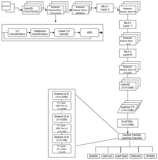
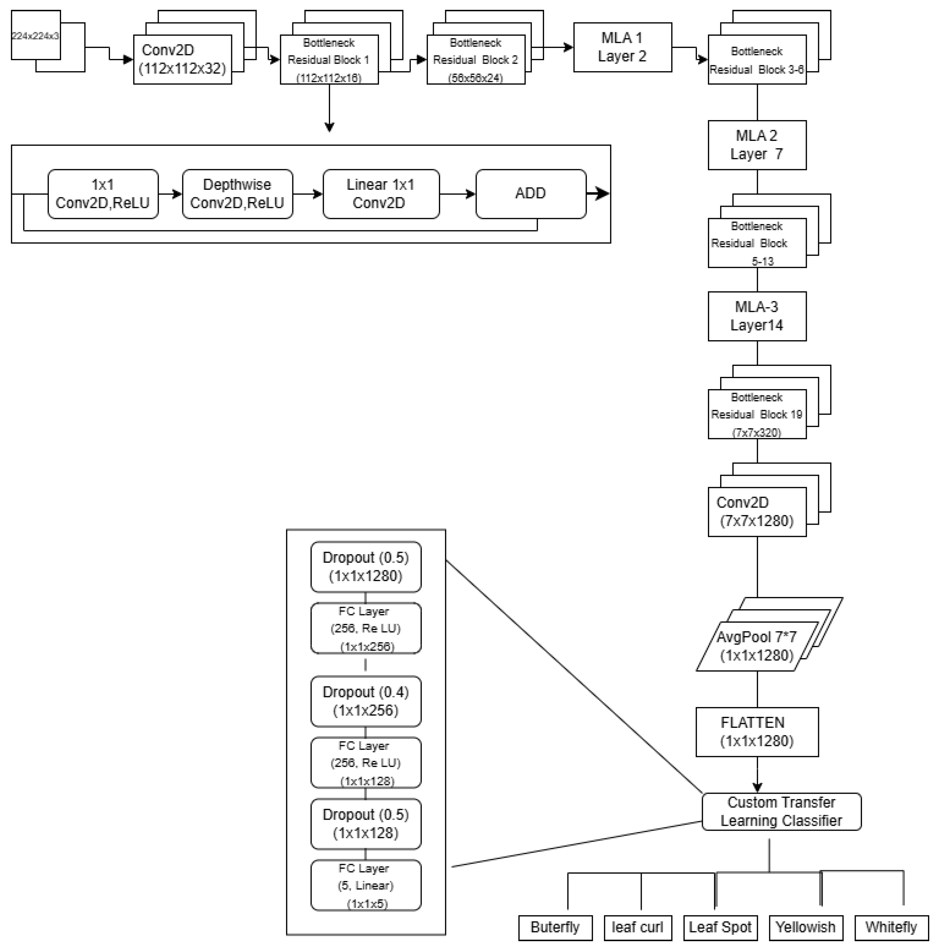
The proposed model aims to classify chili leaf images using a MobileNet with MLA and transfer learning approach as shown in Figure 1. The process starts with input images sized 224 × 224 × 3. These images go through the feature extractor backbone of MobileNetV2 [21], which is a lightweight convolutional neural network architecture pretrained on the ImageNet dataset as it offers a good mix of speed, depth, and performance. This makes it suitable for real-time and resource-efficient detection of plant diseases.

Figure 1. Proposed block diagram.

The first layer of the model applies a standard 2D convolution to the input tensor using a kernel of size k×k. The computational cost is given by Equation (1).

$$h_i·w_i·d_i·d_j·k·k$$

(1)

• $h_i$: height of the input feature map
• $w_i$: width of the input feature map
• $d_i$: number of input channels
• $d_j$: number of output channels
• k: size of the convolution kernel (assumed square, i.e., $k\times k$)

We transform the input tensor of shape $h_i\times w_i\times d_i$ into an output tensor of shape $h_i\times w_i\times d_j$. In practical terms, this corresponds to the transformation of the input image to a feature map using 32 filters, each computing activations over spatial regions and across all input channels, and this is mentioned as per the computational cost. Following this, MobileNetV2 employs depthwise separable convolutions to significantly reduce computational load while preserving feature quality. A depthwise convolution applies a single filter to each input channel, and a subsequent 1 × 1 pointwise convolution combines the outputs across channels. The total cost of this separable processing is given by Equation (2),

$$h_i·w_i·d_i\left(k^2+d_j\right)$$

(2)

making it much more efficient than standard convolution, especially at deeper layers. The core building blocks of the backbone are bottleneck residual blocks, also referred to as inverted residuals with linear bottlenecks. Each block expands the input tensor h × w × $k_t$t → h × w × ($t_k$) convolution with ReLU6 activation. This is followed by a 3 × 3 depthwise convolution with stride s, producing an intermediate tensor of the shape given by Equation (3).

$${\displaystyle \frac{h}{s}}\times {\displaystyle \frac{w}{s}}\times (t·k)$$

(3)

where t = Expansion factor that multiplies input channels in the bottleneck block and finally a linear 1 × 1 projection that brings the tensor back down. The total computation for each such block is given by Equation (4).

$$h·w·d^{\prime }·t\left(d^{\prime }+k^2+d^{″}\right)$$

(4)

encompassing the cost of expansion, spatial filtering, and dimensionality reduction. Throughout these layers, ReLU6 serves as the non-linear activation function [22], defined as shown in Equation (5).

$$\mathrm{ReLU}6\left(x\right)=\min \left(\max (0,x),6\right)$$

(5)

This activation function limits the dynamic range of activations to [0, 6], which has been shown to improve training stability, particularly in low-precision hardware implementations. Notably, ReLU6 is applied after the expansion and depthwise layers, but not after the linear projection in the bottleneck block, preserving its representational capacity. After passing through 19 such bottleneck residual blocks, the output feature map—of shape 7 × 7 × 1280—is processed by a final Conv2D layer and subsequently passed through a Global Average Pooling (GAP) layer. This GAP layer collapses the spatial dimensions by computing the mean of each channel [23] given by Equation (6).

$$y_c={\displaystyle \frac{1}{h·w}}{\displaystyle \sum _{i=1}^h}{\displaystyle \sum _{j=1}^w}{x}_{i,j,c}$$

(6)

This operation yields a 1 × 1 × 1280 tensor, producing a compact global representation of the image. This feature vector, which contains learned meanings, is sent to the custom classification when we have modified the transfer learning layers to extract the detailed features to improve accuracy. In our method, the MobileNetV2 base is used, and the proposed model focuses on chili leaf disease classification while minimizing overfitting on limited data.

In this context, to further strengthen the representation capability of the MobileNetV2 backbone, MLA modules were embedded at strategic positions in the proposed architecture. The MLA blocks were inserted after key transition stages of the network, specifically after feature extraction layers with indices 2, 7, and 14, to refine the feature maps at different abstraction levels. The MLA module strengthens the most informative spatial and channel features while maintaining lightweight computation and stable training. The MLA promotes better localization and generalization by adaptively focusing on salient regions and suppressing the irrelevant background features without affecting the efficiency brought by MobileNetV2. It enhances the capability of the network to precisely focus on the disease-affected region of a chili leaf image with improved classification accuracy and robustness under varying conditions.

3.1. ModifiedLite Attention (MLA)

The Channel Gate (CG) helps the network decide which feature channels carry useful information. The input to this block is a feature map $X\in {\mathbb{R}}^{B\times C\times H\times W}$, where B is the batch size, C is the number of channels, and $H\times W$ represents the spatial size.

To understand the overall contribution of each channel, the CG first applies Global Average Pooling (GAP). This operation simply averages all the values inside a channel, producing one value per channel using Equation (7).

$$g_c={\displaystyle \frac{1}{HW}}{\displaystyle \sum _{i=1}^H}{\displaystyle \sum _{j=1}^W}{X}_{c,i,j}$$

(7)

3.1.1. Channel Gate (CG)

The Channel Gate (CG) helps the network decide which feature channels carry useful information. The input to this block is a feature map $X\in {\mathbb{R}}^{B\times C\times H\times W}$, where B is the batch size, C the number of channels, and H × W the spatial size. To understand the overall contribution of each channel, the CG first applies Global Average Pooling (GAP). This operation simply averages all the values inside a channel, producing one number per channel using Equation (7).

$$g_c={\displaystyle \frac{1}{HW}}{\displaystyle \sum _{i=1}^H}{\displaystyle \sum _{j=1}^W}{X}_{c,i,j}$$

(8)

After global average pooling produces the channel descriptor vector $g\in {\mathbb{R}}^{B\times C}$, this vector acts as a compact summary of how strongly each channel responds to the input feature map. To understand the relationships between channels and determine which ones are important, the Channel Gate passes g through a small two-layer MLP. The first linear layer reduces the channel dimension to a smaller bottleneck, and a SiLU activation $\varphi$ introduces non-linearity while enabling smoother gradients, as shown in Equation (8).

$$S=\sigma \left({\mathrm{PWConv}}_{1\times 1}\left(U\right)\right)$$

(9)

The second linear layer then expands this reduced representation back to the original channel dimension. Formally, the transformations are given by Equation (9).

$$z=\varphi (g{W}_1+b_1),q=z{W}_2+b_2$$

(10)

The vector z captures essential cross-channel interactions in the compressed space, while q contains the raw importance scores for all C channels. A sigmoid activation is then applied to q to convert these scores into attention weights C = $\sigma \left(q\right)$, ensuring that each channel receives a value between 0 and 1. These weights are reshaped to [B,C,1,1] and broadcast across the spatial dimensions of the feature map, allowing the network to boost channels that contain useful disease-related features and suppress those that contribute less to the final prediction.

3.1.2. Spatial Gate (SG)

The Spatial Gate identifies where the most relevant evidence is located within the feature map. Its input is the tensor $X\in {\mathbb{R}}^{B\times C\times H\times W}$, which represents the output of the preceding CNN layer with B samples, C feature channels, and spatial dimensions $H\times W$. To generate spatial attention, MLA applies a lightweight mechanism inspired by MobileNet. First, a depthwise $3\times 3$ convolution is applied independently to each channel of X, and the result is passed through a Si LU activation, producing an intermediate feature map U. This step allows the model to capture local structures such as lesion edges, infected spots, and texture variations across the leaf surface. Next, a pointwise 1 × 1 convolution compresses the channel dimension of U into a single spatial map. A sigmoid activation is then applied to normalize the output into the range [0, 1], yielding the final spatial attention mask S. Formally, this process is expressed as

$$U=\varphi \left({\mathrm{DWConv}}_{3\times 3}\left(X\right)\right)$$

(11)

3.1.3. Edge Prior (EP)

The Edge Prior branch introduces structural information into the attention mechanism without adding any learnable parameters. Its goal is to highlight sharp intensity transitions, contours, and boundary details that often correspond to disease symptoms on leaf surfaces.

Given the input feature map $X\in {\mathbb{R}}^{B\times C\times H\times W}$, MLA first forms a grayscale proxy by averaging over the channel dimension, producing $\overline{X}\in {\mathbb{R}}^{B\times 1\times H\times W}$. This removes channel specific variations and retains the overall structural layout.

Classical edge-detection filters are then applied to $\overline{X}$. Horizontal and vertical Sobel kernels extract gradient responses $G_x$ and $G_y$, while a Laplacian kernel produces the second-order response L, which is sensitive to abrupt intensity changes. The gradient magnitude and Laplacian are combined to form the raw edge map:

$$M_e=\sqrt{G_x^2+G_y^2}+\left|L\right|$$

(12)

Because the strength of edges can vary from image to image, $M_e$ is normalized on a per-sample basis to obtain a stable attention signal:

$$E={\displaystyle \frac{M_e-\min \left(M_e\right)}{\max \left(M_e\right)-\min \left(M_e\right)+ϵ}}$$

(13)

The resulting map $E\in {[0,1]}^{B\times 1\times H\times W}$ emphasizes high-frequency structures such as lesion outlines, vein distortions, and irregular edges. This Edge Prior guides the attention mechanism toward meaningful structural cues, helping the model better localize disease-affected regions that may not be fully captured by channel or spatial attention alone.

3.1.4. Weighted Fusion and Residual Scaling

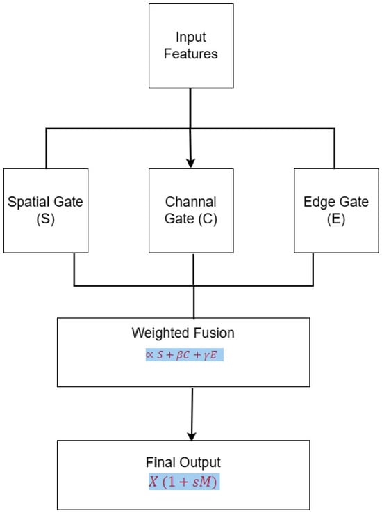
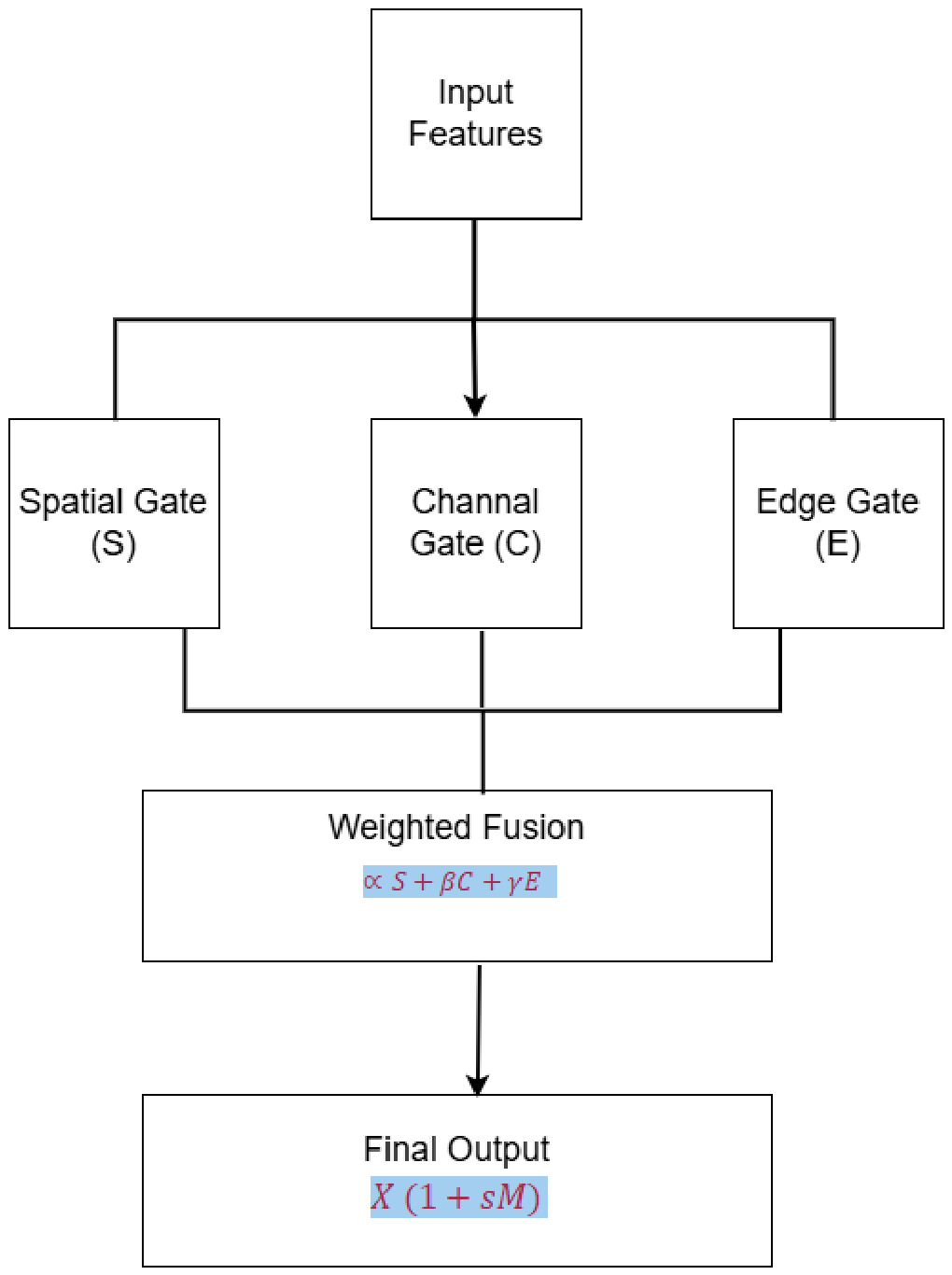
After generating channel-wise, spatial, and edge-based attention maps, MLA combines these complementary cues through a lightweight fusion mechanism as shown in Figure 2. Each branch contributes differently, so MLA introduces three learnable scalar weights—$\alpha$, $\beta$, and $\gamma$—to control their relative influence. In our implementation, all three scalars are initialized to $0.5$, giving equal importance to the Channel Gate, Spatial Gate, and Edge Prior at the start of training. This balanced initialization prevents the model from favoring one branch prematurely and allows the network to learn the optimal contribution of each attention pathway directly from data.

Figure 2. Modified light attention model.

The fused attention signal is computed as:

$$M=\sigma (\alpha S+\beta C+\gamma E),$$

(14)

where $\sigma$ denotes the sigmoid function, which normalizes the output to the range $[0,1]$. The resulting unified attention mask $M\in {(0,1)}^{B\times 1\times H\times W}$ highlights regions and features consistently reinforced by spatial saliency, channel statistics, and structural edge cues.

To ensure stable integration with the pretrained MobileNetV2 backbone, MLA applies this fused mask using a residual scaling strategy. Instead of modifying the features abruptly, a single learnable scalar s, initialized to zero, controls the strength of the refinement. The final output is expressed as:

$$Y=X\times (1+s\times M),$$

(15)

With $s=0$ at initialization, the block behaves as an identity mapping, ensuring that pretrained weights are not disturbed in early training. As learning progresses, s gradually increases, enabling MLA to selectively amplify informative regions while keeping computation minimal. This residual formulation allows MLA to improve feature quality smoothly and reliably across different layers of the network.

3.2. Proposed Transfer Learning Layer

To adapt the pretrained MobileNetV2 backbone for multiclass classification on the chili leaf dataset, a custom classifier head is appended on top of the base network. This classifier head leverages the high-level features extracted by MobileNetV2 and fine-tunes them for domain-specific classification. After the $7\times 7$ average pooling operation reduces the spatial dimensions of the feature map, the output from MobileNetV2 becomes a $1\times 1\times 1280$ dimensional global feature vector. This vector serves as the input to the transfer learning head.

The transfer learning head consists of a sequence of Fully Connected (FC) layers interleaved with dropout layers, designed to progressively refine the extracted features and prevent overfitting. This configuration enables the model to learn non-linear decision boundaries suitable for the target classification task.

3.2.1. Dropout Layer

Dropout, which Srivastava et al. [24] first suggested, is the key way that the classifier head protects itself from overfitting. This technique injects randomness during training by suppressing a subset of neurons to prevent co-adaptation and promote more robust feature representations. Formally, dropout is defined as

$$Y_i={\displaystyle \frac{X_i·M_i}{1-p}}$$

(16)

where

• p: Dropout rate (e.g., $0.5,0.4,0.3$)
• $Y_i$: Output of neuron i after dropout
• $X_i$: Input to neuron i (before dropout)
• $M_i$: Random mask for neuron i; either 1 (keep with probability $1-p$), or 0 (drop with probability p)

The feature vector of size $1\times 1\times 1280$ is processed sequentially by dropout layers of rates $0.5$, $0.4$, and $0.3$ in our architecture. This configuration enforces strong regularization on the high-dimensional representation while maintaining its dimensionality since dropout modifies neuron activation and does not affect the structural size of the feature vector. During inference, dropout is disabled and all neurons are active to ensure fixed behavior, which is consistent with what was expected in the training phase.

3.2.2. Fully Connected Layers

Fully Connected (FC) or dense layers represent the main decision-making elements of the classifier head [25]. This idea of connecting each neuron to every input and learning these weights using backpropagation is from Rumelhart et al. [26]. Following the generation of the feature map by the MobileNetV2 backbone, a $7\times 7$ average pooling generates a $1\times 1\times 1280$ global feature representation, which constitutes the input to a set of FC layers that gradually refine and specialize this representation for multiclass classification. An FC layer is defined as

$$y=f(Wx+b)$$

(17)

where

• $x\in {\mathbb{R}}^n$: Input vector to the layer
• $W\in {\mathbb{R}}^{m\times n}$: Weight matrix
• $b\in {\mathbb{R}}^m$: Bias vector
• $f(·)$: Activation function (e.g., ReLU)
• $y\in {\mathbb{R}}^m$: Output of the layer with m neurons

A linear transformation is carried out in the expression $Wx+b$, after which a nonlinear operation f follows; hence, the network learns how the complete set of high-level features together contributes to the final classification.

3.2.3. Softmax Layer

The softmax activation function [25] is used to convert these logits into interpretable class probabilities. By normalizing the outputs to fall between $[0,1]$ and sum to 1, this function makes them appropriate for probabilistic interpretation. The softmax function is defined as follows:

$$p_i={\displaystyle \frac{e^{z_i}}{{\sum }_{j=1}^C{e}^{z_j}}},i\in \{1,2,\dots ,C\}$$

(18)

The cross-entropy loss is used to compare the model’s prediction with the actual class label after the output logits have been transformed into class probabilities using the softmax function. This loss function quantifies the model’s performance in a probabilistic sense by calculating the difference between the actual (ground-truth) class distribution and the anticipated probability distribution. In practice, models are trained on batches of samples rather than a single input at a time. To compute the loss over a batch of N samples, the cross-entropy losses of all individual samples are averaged. This gives the batch-averaged cross-entropy loss:

$$L_{\mathrm{avg}}=-{\displaystyle \frac{1}{N}}{\displaystyle \sum _{n=1}^N}\log \left(p_{k_n}^{\left(n\right)}\right)$$

(19)

• N: Number of samples in the batch
• $k_n$: True class label of the n-th sample
• $p_{k_n}^{\left(n\right)}$: Predicted probability for the true class of the n-th sample after applying softmax

This averaging ensures that the gradient updates during training reflect the performance across the entire batch, rather than being dominated by a single sample. It also improves training stability and allows the model to generalize better.

4. Experiment Results and Analysis

This section presents the experimental outcomes. It starts with a detailed description of the dataset, the specific model architecture and training settings, and the evaluation metrics employed. Following this, comparative analyses are performed to thoroughly assess the effectiveness of the proposed classification model.

4.1. Construction of the Dataset

The dataset used in this study was compiled from Kaggle [27]. It contains images from five categories: leaf spot, leaf curl, whitefly, yellowish leaves, and healthy leaves. The transformations such as rotation, zoom, brightness adjustment, and horizontal/vertical flipping were performed to create the dataset used of 4432 image samples as shown in Table 1. The images were preprocessed and converted into NumPy arrays and subsequently transformed into tensors for model training. The dataset was randomly split into training, validation, and test sets in 75:15:10 ratios to maintain a balanced distribution across all classes. The numbers of separate experimental runs up to 20 were performed and possible best results were considered. The model was trained for 100 epochs using the Adam optimizer with a learning rate of 0.0001 and a weight decay of 0.0001. The batch size was set to 32, and a ReduceLROn Plateau scheduler was used to reduce the learning rate when the validation loss plateaued.

Table 1. Dataset details.

Disease Class	Training Set	Validation Set	Testing Set
Healthy	480	96	64
Leaf spot	1044	208	140
Whitefly	600	120	80
Yellowish	600	120	80
Leaf curl	600	120	80
Total	3324	664	444

4.1.1. Hardware and Software Environment

The implementation of the proposed model was carried out using PyTorch 2.1.0 and Python 3.10, executed on a Windows 11 operating system. The hardware platform comprised an NVIDIA RTX 3060 GPU with CUDA 12.6 support, enabling efficient parallel computation and accelerated model training. The software environment was configured with a comprehensive suite of Python libraries, including NumPy for numerical operations, Matplotlib 3.10.x for data visualization, and scikit-learn for performance evaluation metrics. PyTorch modules were utilized extensively for model construction, training, regularization, and optimization. This combination of hardware and software resources provided a stable and high-performance environment for the development and evaluation of the deep learning model.

4.1.2. Evaluation Metrics

The performance of the classification model is assessed using several standard evaluation metrics [28] shown from Equation (20) to Equation (24), which provide insight into its ability to correctly distinguish between the two classes. The key measures considered include accuracy, precision, recall (sensitivity), F1-score, specificity, and the precision–recall curve. These metrics collectively help in understanding both the overall prediction accuracy and the model’s effectiveness in identifying positive and negative cases.

The mathematical definitions of these metrics are as follows:

$$\mathrm{Accuracy}={\displaystyle \frac{TP+TN}{TP+TN+FP+FN}}\times 100$$

(20)

$$\mathrm{Precision}={\displaystyle \frac{TP}{TP+FP}}\times 100$$

(21)

$$\mathrm{Recall}={\displaystyle \frac{TP}{TP+FN}}\times 100$$

(22)

$$\mathrm{F}1\text{-}\mathrm{Score}={\displaystyle \frac{2\times (\mathrm{Precision}\times \mathrm{Recall})}{\mathrm{Precision}+\mathrm{Recall}}}\times 100$$

(23)

$$\mathrm{Specificity}={\displaystyle \frac{TN}{TN+FP}}\times 100$$

(24)

Here, false negatives (FN) are positive samples that are mistakenly predicted to be negative, false positives (FP) are negative samples that are mistakenly labelled as positive, true negatives (TN) are negative samples that are accurately identified, and true positives (TP) indicate the number of samples that are correctly classified as belonging to the positive class. To ensure that the model can be used effectively in real-world applications without excessive computational cost, computational efficiency and model complexity are also assessed.

4.2. Model Performance Evaluation

In this study, the proposed MobileNetV2 model is evaluated under two distinct scenarios aimed at robustly assessing its effectiveness in chili plant disease detection.

Scenario 1: In this scenario, individual diseases are evaluated against healthy leaves to demonstrate how accurately the model differentiates between healthy leaves and specific diseases. Two cases are considered: leaf curl and whitefly disease.

Case 1: Evaluation of Leaf Curl and Healthy Leaves.

In this experiment, the study used transfer learning with MobileNetV2 as the backbone. The feature extraction layers were frozen, and the final classification layer was replaced with a fully connected layer containing two output neurons for binary classification (“leafcurl” and “healthy”). The model was trained for 100 epochs using the Adam optimizer with a learning rate of 0.0001 and a weight decay of 0.0001. The batch size was set to 32, and a Reduce LROn Plateau scheduler was used to reduce the learning rate when the validation loss plateaued. The proposed method obtained good results with respect to all parameters compared to other methods such as Squeezenet, Shufflenet, Efficientnet, Xception and MobilenetV2 as shown in Table 2.

Table 2. Classification results of leaf curl and healthy.

Model	Training Accuracy	Training Loss	Validation Accuracy	Validation Loss	Test Accuracy	Test F1-Score
SqueezeNet	0.9751	0.1121	0.9714	0.1267	0.9433	0.9432
ShuffleNet	0.9291	0.3916	0.9381	0.3865	0.9504	0.9498
EfficientNet	0.9330	0.3937	0.9381	0.3871	0.9574	0.9571
MnasNet	0.9397	0.2279	0.9143	0.3244	0.9078	0.9062
MobileNetV2	0.9800	0.0912	0.9810	0.0928	0.9645	0.9645
Proposed Model	0.9866	0.0421	0.9905	0.0214	0.9929	0.9929

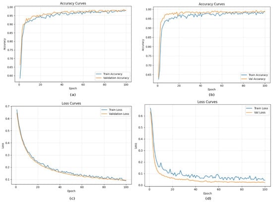
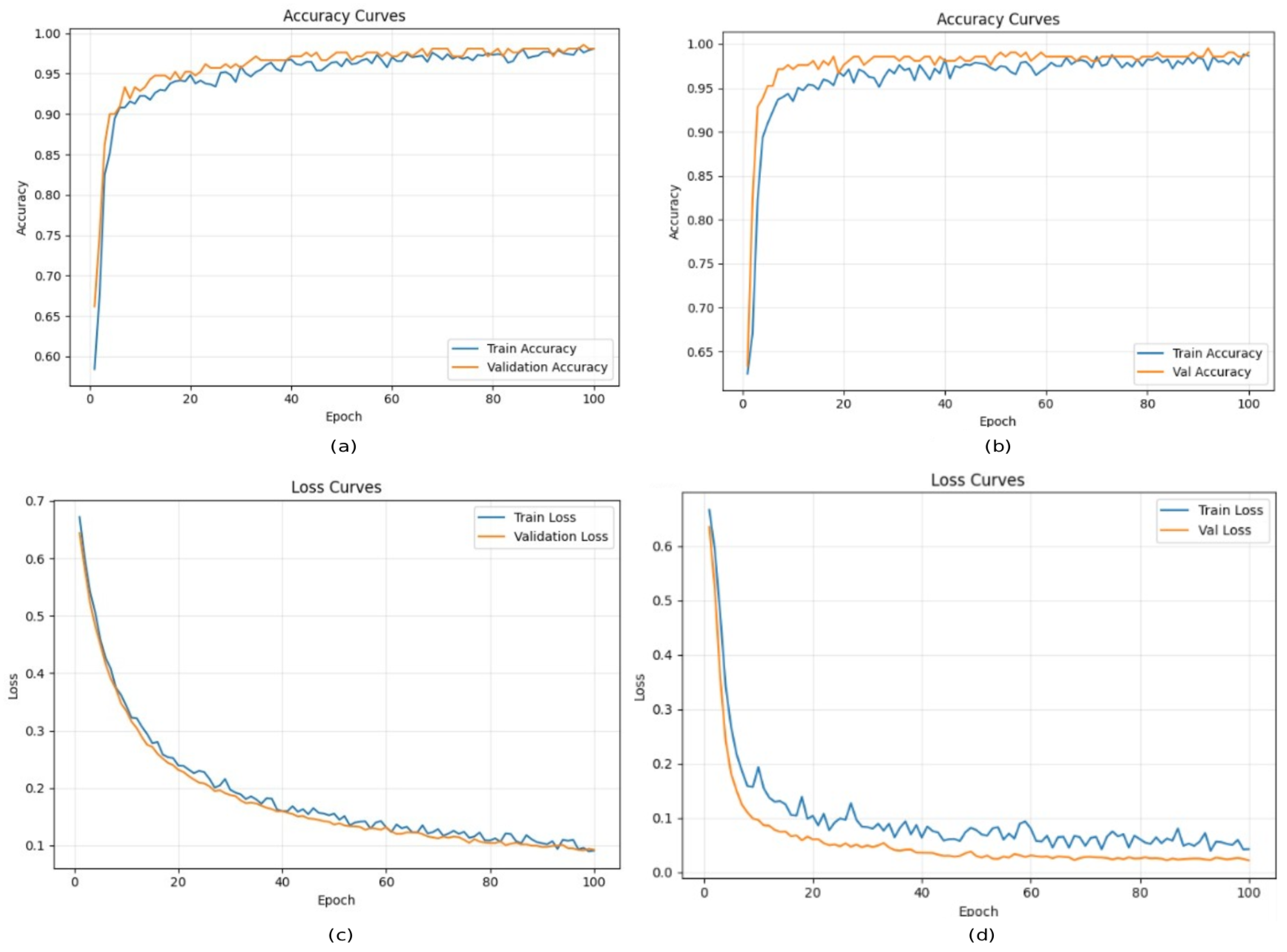
The training and validation curves for accuracy and loss are shown in Figure 3a–d. The training process reached a final training accuracy of 98.66% and a validation accuracy of 99.05%. After training, the model was evaluated on the held-out test set, achieving a test accuracy of 99.29% and a weighted F1-score of 0.9929.

Figure 3. (a–d): Accuracy and loss curves for leaf curl and healthy leaves.

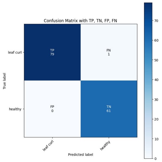
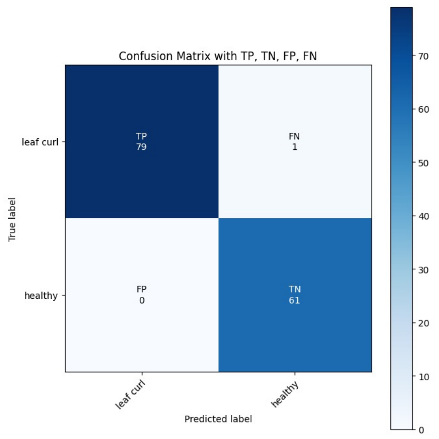
The confusion matrix for the test set is shown in Figure 4, with true positives, false positives, true negatives, and false negatives annotated. The per-class accuracy was 98.75% for the “leafcurl” class and 100% for the “healthy” class, confirming that the model generalizes well to unseen data. These results demonstrate that the proposed transfer learning approach with MobileNetV2 is highly effective in classifying leaf curl vs. healthy leaves.

Figure 4. Confusion matrix.

Case 2: Evaluation of Whitefly Disease and Healthy Leaves.

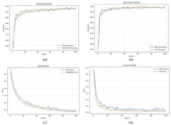
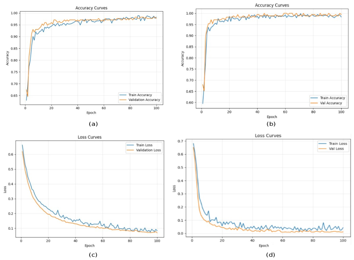
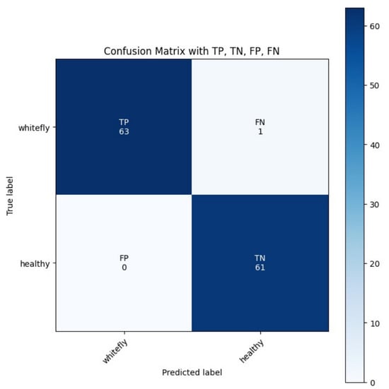
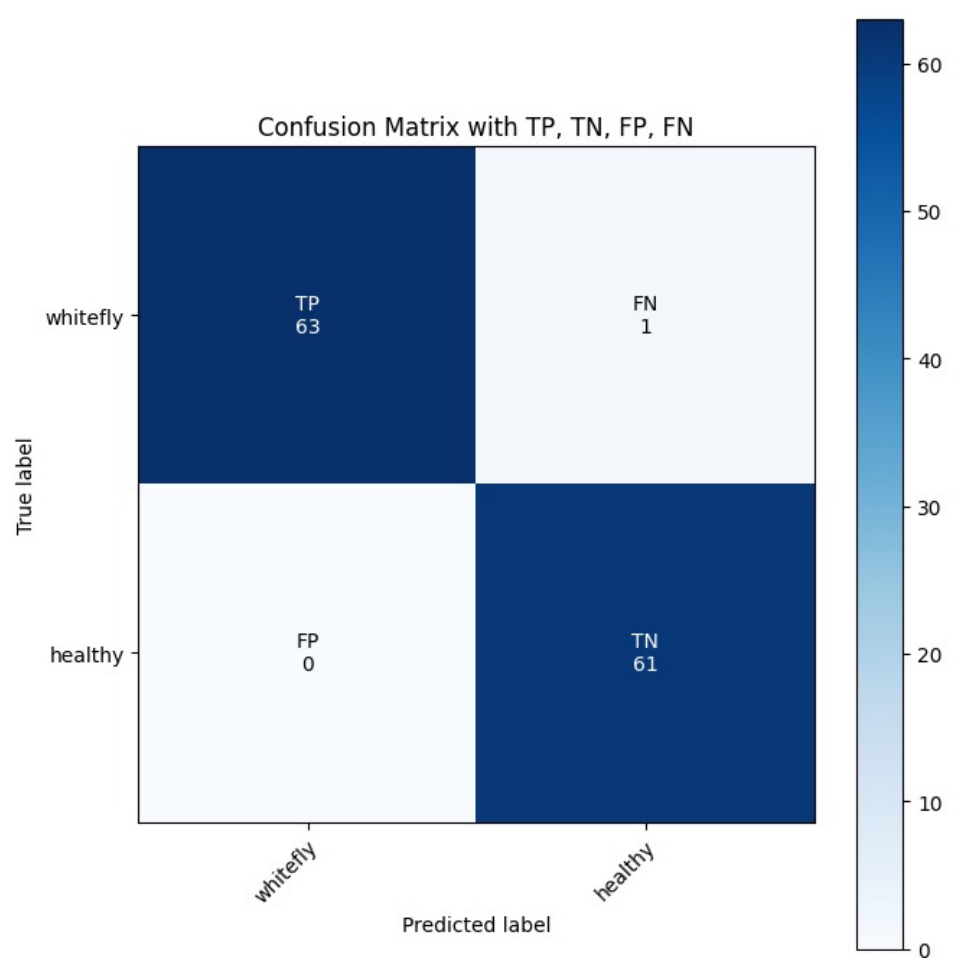
In this experiment, transfer learning with MobileNetV2 is used as the backbone. The feature extraction layers are frozen, and the final classification layer is replaced with a fully connected layer containing two output neurons for binary classification (“whitefly” and “healthy”). The model is trained for 100 epochs using the Adam optimizer with a learning rate of $0.0001$ and a weight decay of $0.0001$. The batch size is set to 32, and a ReduceLROnPlateau scheduler is used to reduce the learning rate when the validation loss plateaus. The proposed method obtained good results with respect to all parameters compared to other methods such as Squeezenet, Shufflenet, Efficientnet, Xception and MobilenetV2 as shown in Table 3. The training and validation curves for accuracy and loss are shown in Figure 5a–d. The confusion matrix for the test set is shown in Figure 6.

Table 3. Classification results of whitefly and healthy.

Model	Train Acc	Train Loss	Val Acc	Val Loss	Test Acc	F1-Score
SqueezeNet	0.9745	0.0840	0.9535	0.0965	0.9600	0.9600
ShuffleNet	0.9356	0.3687	0.9419	0.3413	0.9440	0.9439
EfficientNet	0.9329	0.3642	0.9302	0.3471	0.9360	0.9358
MnasNet	0.9463	0.2009	0.9302	0.2793	0.9520	0.9518
MobileNetV2	0.9826	0.0840	0.9767	0.0695	0.9760	0.9760
Proposed Model	0.9839	0.0431	0.9942	0.0115	0.9920	0.9920

Figure 5. (a–d): Accuracy and loss curves for whitefly and healthy leaves.

Figure 6. Confusion matrix.

Scenario 2: Multiclass Classification.

This scenario uses the same hyperparameters as Scenario 1. These include a modified classifier head with five output neurons and mean normalization of input images. Using transfer learning and fine-tuning, the model was trained with the following hyperparameters: 100 epochs, Cross Entropy Loss as the loss function, Adam optimizer (learning rate $=0.0001$, weight decay $=0.0001$), and a batch size of 32. A Reduce LROn Plateau scheduler was employed to reduce the learning rate when the validation loss plateaued, using a factor of 0.5 and a patience of 5 epochs.

The MobileNetV2 architecture with transfer learning demonstrated better performance compared to baseline CNN models. To ensure a fair comparison, the same set of hyperparameters was used across all models. The proposed method achieved superior results across all evaluation metrics compared to other methods such as SqueezeNet, ShuffleNet, EfficientNet, Xception, and MobileNetV2, as shown in Table 4.

Table 4. Classification results of 5 classes: leaf spot, leaf curl, whitefly, yellowish, and healthy.

Model	Train Acc	Train Loss	Val Acc	Val Loss	Test Acc	F1-Score
SqueezeNet	0.9415	0.2032	0.9210	0.2441	0.9176	0.9173
ShuffleNet	0.8234	0.7436	0.8250	0.7280	0.8071	0.7982
EfficientNet	0.9344	0.2283	0.9355	0.1887	0.9176	0.9172
MnasNet	0.9435	0.1894	0.9097	0.2791	0.8753	0.9201
MobileNetV2	0.9522	0.1896	0.9419	0.2128	0.9200	0.9201
Proposed Model	0.9435	0.1605	0.9742	0.0824	0.9624	0.9622

The findings indicate that the suggested MobileNetV2-based architecture outperformed the other CNN architectures, achieving around 96% classification accuracy on the five-class dataset under the confusion matrix for the four classes.

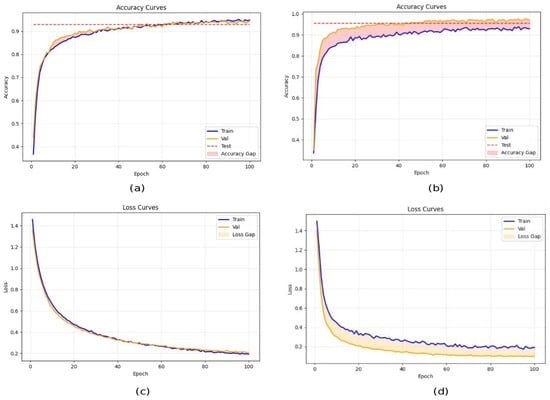
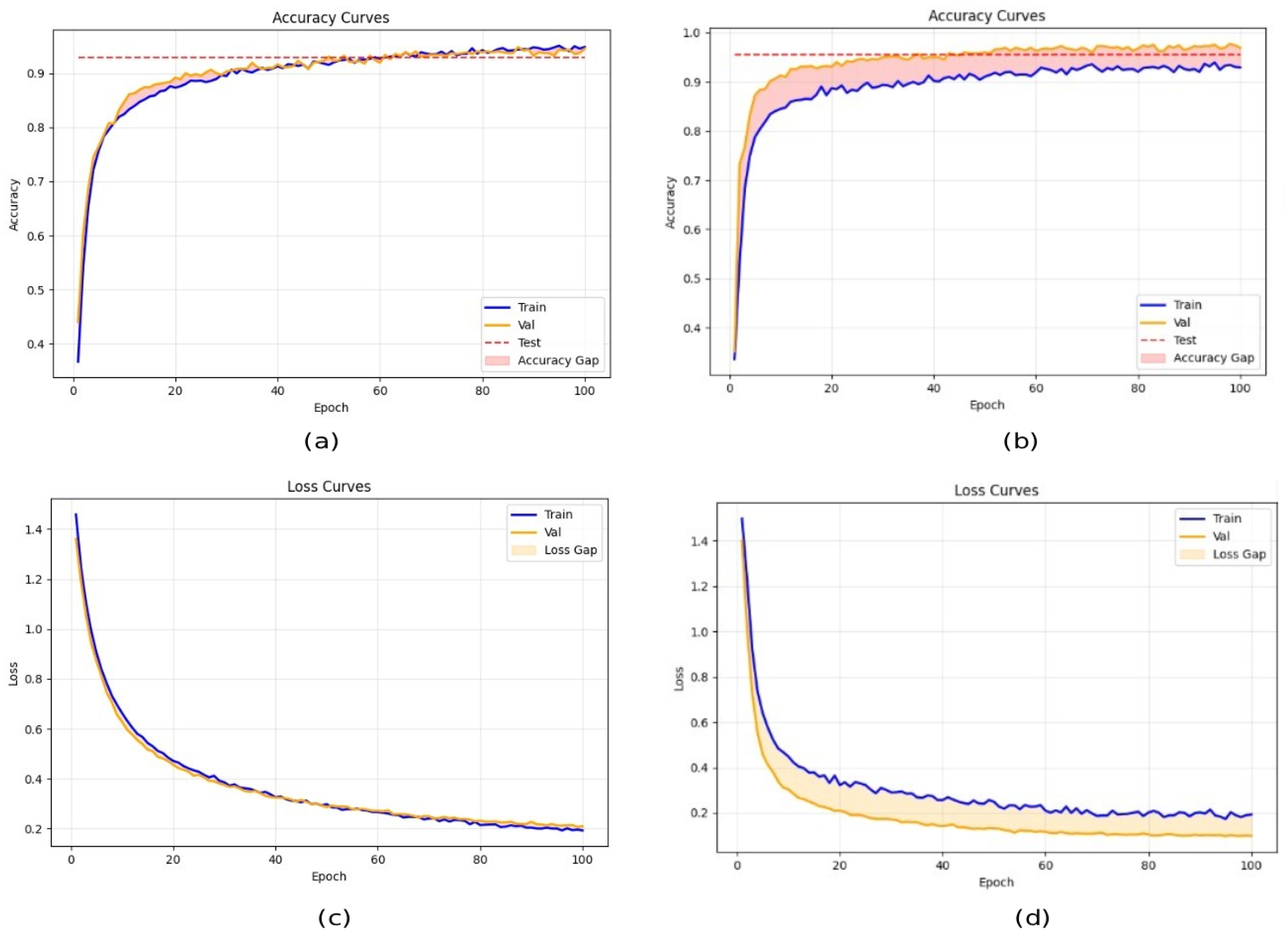
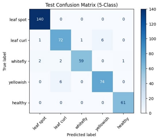
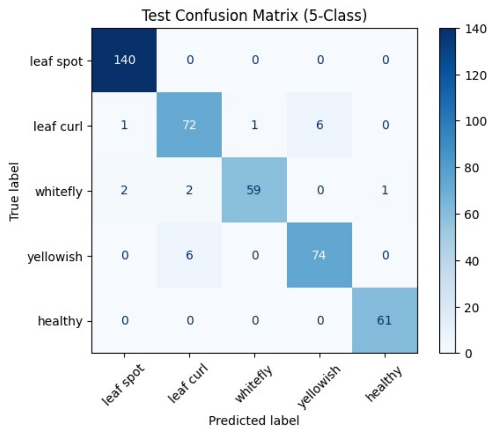
Figure 7 shows the accuracy and loss during training in Scenario 2, demonstrating the model’s ability to generalize well to unseen data and its confusion matrix is shown in Figure 8. Deeper understanding of the model’s performance across all five categories is possible thanks to the per-class accuracies. The model’s 100% accuracy in accurately classifying leaf spot and healthy leaves, as demonstrated by the confusion matrix, indicates excellent discrimination for these two groups. With a 95.00% classification accuracy, the yellowish class performed well but marginally less than the ideal classes. The accuracy rates for the leaf curl and whitefly classes were 90.00% and 93.75%, respectively. These somewhat lower results imply that these classes might be more difficult to classify due to more difficult intra-class variations or visual resemblances to other categories. With all accuracies above 90%, the model continuously performs well across all classes, according to the overall results, suggesting that it is a very reliable and broadly applicable classification model.

Figure 7. (a–d): Accuracy and loss curves for whitefly and healthy leave.

Figure 8. Confusion matrix.

4.3. Disscussion

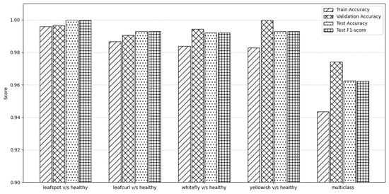
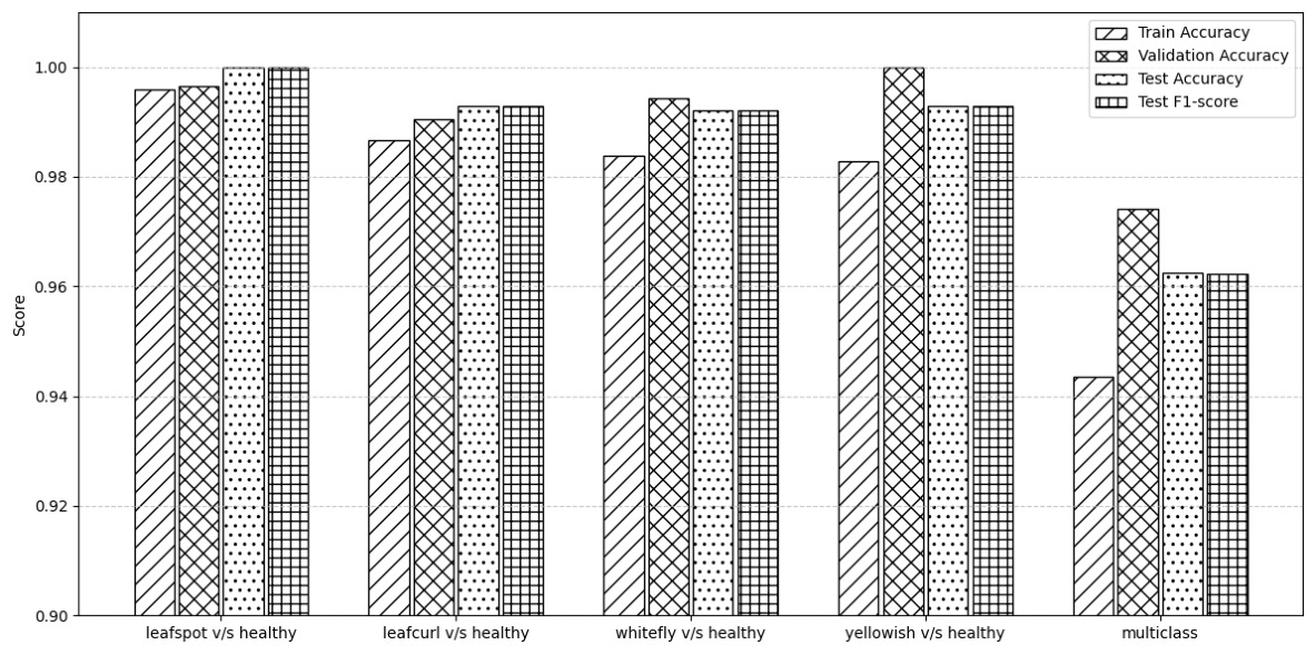
The actual outcomes exceeded the goal performance level of 90%, and all prediction cases had accuracy values over that threshold. While the whitefly vs. healthy categorization obtained 99.20%, the findings of Scenario 1’s differentiation between healthy instances and leaf curl reached 99.29%. The model maintained good accuracy even though these two disease classes presented slightly more difficulties because of intra-class variances and visual similarities. These results show how well the suggested MobileNetV2-based method generalizes to data on chili leaf disease that has not yet been observed. Compared to simpler binary classification tasks, Scenario 2’s training of four disease categories and healthy leaf cases presented greater complexity and took longer. Even with the added complexity, the suggested model performed exceptionally well in identifying these particular chili leaf diseases. Training, validation, test accuracies, and F1-scores are among the important performance measures that are compiled in Figure 9 for every experimental scenario. The experimental findings confirm that the suggested method for detecting plant diseases is reliable. The model obtained a nearly matching F1-score of 0.9622 and a high test accuracy of 96.24% in the multiclass classification including four disorders. The model achieved near-perfect test accuracies and F1-scores for the binary disease vs. healthy classifications: “leafspot vs. healthy” achieved 100% accuracy and F1-score; “leafcurl vs. healthy” achieved 99.29%; “whitefly vs. healthy” and “yellowish vs. healthy” reached 99.20% and 99.29%, respectively. These findings support the model’s high efficacy for tasks involving the identification of single diseases as well as multi-disease discrimination. Gradient-weighted Class Activation Mapping (Grad-CAM) is a visualization technique that generates class-specific localization maps to highlight regions in an image that contribute most to a model’s decision [29]. It computes the gradients of the target class score $y_c$ with respect to the final convolutional feature maps $A^k\in {\mathbb{R}}^{H\times W}$, and uses them to obtain importance weights as shown in Equation (25)

$${\alpha }_k^c={\displaystyle \frac{1}{H\times W}}\sum _i\sum _j{\displaystyle \frac{\partial y_c}{\partial A_{ij}^k}}$$

(25)

Figure 9. Bar graph comparing different scenarios.

The class-discriminative localization map is then given by:

$$L_c=\mathrm{ReLU}\left(\sum _k{\alpha }_k^c{A}^k\right)$$

(26)

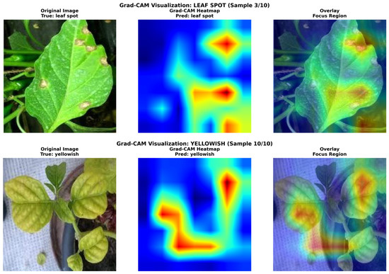
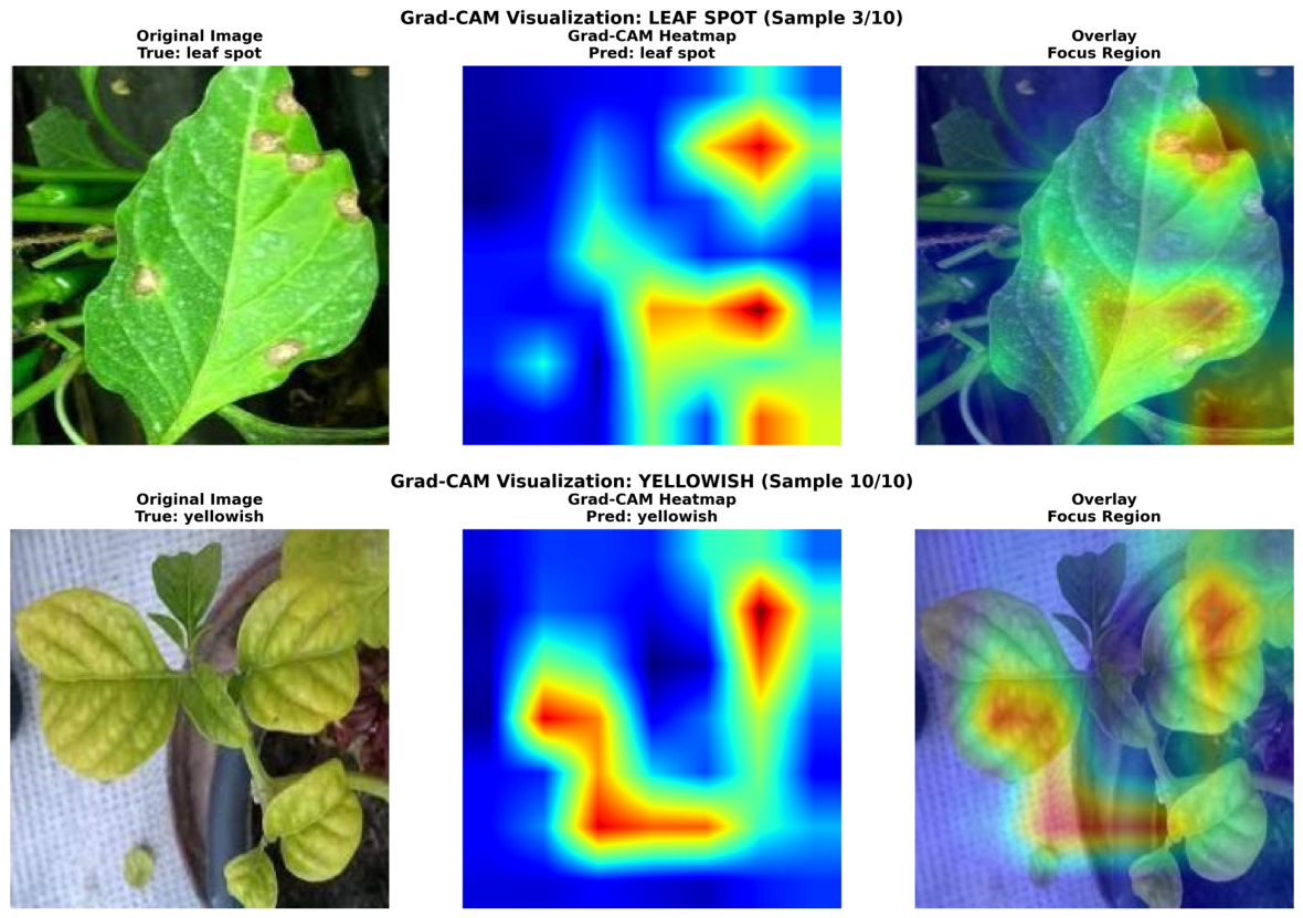
This activation map $L_c$ is upsampled to the input resolution for visualization. Utilizing the last convolutional layer provides an effective trade-off between high-level semantic representation and spatial resolution, while the ReLU operation ensures that only features positively influencing the target class are retained, producing interpretable and non-negative heat maps. To evaluate the interpretability of the model, Grad-CAM was utilized to generate class-discriminative heatmaps for the anticipated labels in the final convolutional block of the MobileNetV2 backbone. These heatmaps show spatial areas that improve the classification outcome, with warmer colors denoting stronger activation that correlates to the model’s confidence. As seen in Figure 10, the “leaf spot” Grad-CAM image concentrates strong activation over clustered necrotic lesions. This confirms that the model focuses on regions that are particular to symptoms and is compatible with the morphological aspects of the disease. In contrast, the “yellowish” image illustrates the diffuse staining pattern that is characteristic of these symptoms, with larger activation throughout several leaflets in the chlorotic lamina.

Figure 10. Grad-CAM sample image out.

4.4. Model Interpretability Using Grad-CAM

The Grad-CAM visualization findings for plant disease detection are shown in Figure 10, which highlights the particular leaf sections that have a major impact on the model’s prediction. The suggested model successfully learns disease-relevant features rather than background information, as evidenced by the heatmap’s obvious focus on affected areas like discolouration, patches, curls, and degraded textures.

4.5. Ablation Studies

An ablation study was performed to investigate the relative importance of each subcomponent within the proposed Modern Lite Attention (MLA) module. The study aimed to determine how the Channel Gate, Spatial Gate, and Edge Prior contribute individually to the overall performance. All experiments were conducted using the same training protocol and the MobileNetV2 backbone as the base model. The corresponding quantitative results are presented in Table 5. The baseline MobileNetV2 model achieved an accuracy of 93.12% and an F1-score of 0.912. Integrating the complete MLA module led to a significant performance improvement, reaching 97.84% accuracy and an F1-score of 0.976, while adding only a minimal increase in parameters (from 3.47 M to 3.85 M) and FLOPs (from 300 M to 322 M). When the Edge Prior branch was removed, the accuracy dropped to 96.21%, indicating that structural edge cues play an important role in refining lesion boundaries and enhancing detail awareness.

Table 5. Ablation studies.

Variant	Accuracy (%)	F1-Score	Params (M)	FLOPs (M)
MobileNetV2 (Baseline)	93.12	0.912	3.47	300
Channel gate + Spatial gate	96.21	0.962	3.74	318
Spatial gate + Edge prior	95.46	0.953	3.72	316
Channel gate + Edge prior	95.02	0.947	3.70	315
Only Edge Prior	94.25	0.935	3.68	312
Proposed model	97.84	0.976	3.85	322

Excluding the Channel Gate reduced performance further to 95.46%, confirming its importance in recalibrating feature responses and enhancing channel-wise selectivity. Similarly, removing the Spatial Gate led to an accuracy of 95.02%, showing that spatial attention contributes strongly to localizing disease regions across leaf surfaces. The Only Edge Prior variant, which retains only contour and gradient-based information, achieved 94.25% accuracy and 0.935 F1-score. This comparatively lower result demonstrates that edge information alone is insufficient for robust classification, emphasizing the complementary roles of all three components. Overall, these results validate that each submodule within MLA contributes uniquely to improving feature representation, and their combined operation yields the best balance of accuracy, interpretability, and efficiency.

4.6. Comparison with Existing Attention Modules

The excitation process [30] uses the data gathered in the squeeze to completely capture the channel dependencies, where a straightforward gating uses a sigmoid activation method. This focuses solely on channel relationships where Excessive “soft” weighing of all input entities can result in significant computing costs. Unless they are significantly altered, as in non-local networks, SE modules only process local neighborhoods or channel-wise information, which may restrict their capacity to capture long-range global dependencies.

The Convolutional Block Attention Module (CBAM) [31], which uses dual-channel and spatial attention processes to improve the model’s capacity to capture texture, edges, and spatial distribution properties of diseased regions, is incorporated using the SinGAN framework as the baseline. In order to assess the enhancement provided by channel-wise attention mechanisms, a SinGAN-SE model is also built for comparative research. Key category recognition performance approaches or surpasses 0.98, and downstream classification results show that the YOLOv8 model trained on data produced by SinGAN CBAM achieves superior precision, recall, and F1-score to those trained with other models. To compress features, CBAM primarily uses global average and max pooling. Fine-grained spatial and channel-wise information, which is essential for tasks like medical imaging or small target recognition, may be lost as a result of this process.

The initial spatial attention module usually makes use of a convolutional kernel. Some studies use dilated convolutions to increase the receptive field because this fixed size might not adequately capture bigger multi-scale contextual interactions. In [32], the PlantVillage dataset is used to evaluate aECA-ResNet34 with several plant disease classification models. According to the experimental findings, the aECA-ResNet34 model suggested performs better, is more resilient, and has greater accuracy. The findings demonstrate how well the aECA-ResNet34 model presented in this study can identify illnesses of several plant leaves. But ECA-Net does not offer spatial (pixel-wise) attention because it is a dedicated channel attention mechanism. It ignores the location of the information, which is essential for tasks like object localization, and simply considers feature importance across channels. In [33], they utilize an SDM-Net model that combines self-distillation with a CAA attention mechanism. The use of the self-distillation method with depthwise separable convolution to create an adaptive learning module that allows the model to retain high recognition accuracy and robustness is challenging. According to the findings, the SDM-Net model’s recognition accuracy was 93.49% with an accuracy of 89.08%. The suggested MLA works across several hierarchical layers, in contrast to the above-discussed techniques, which apply attention in a more aggregated fashion. This leads to better discriminative representations by allowing the model to simultaneously modify high-level semantic features and low-level structural elements (such as edges and textures). In particular, this shows that subtle edge distortions and also irregular lesion patterns are indicative of early-stage diseases, where class separability and localization are enhanced by boundary information.

As summarized in Table 6, the baseline MobileNetV2 achieved an accuracy of 95.91% with an F1-score of 0.958. Surprisingly, the addition of the SE block decreased accuracy to 91.68%, indicating that channel-only recalibration is not sufficient for this dataset. SE models only evaluate global channel statistics through spatial pooling, which causes the loss of fine local lesion patterns—leading to weaker discrimination in plant disease images. Similarly, the ECA module achieved 82.62% accuracy and an F1-score of 0.816, demonstrating that while ECA introduces efficient local channel interaction, its fixed 1D kernel size restricts adaptability across varying feature scales. As a result, important spatial cues such as texture irregularities and boundary distortions are inadequately captured. CBAM also exhibited reduced performance, achieving only 86.10% accuracy. In contrast, SDMnet achieved 96.91% accuracy and an F1-score of 0.967, outperforming SE, ECA, and CBAM. SDMnet benefits from its parallel channel–spatial attention pathways; however, its large receptive fields tend to generate coarse attention responses that overlook small, irregular lesion regions. The proposed MobileNetV2 + MLA module delivered the best performance, achieving 97.84% accuracy and an F1-score of 0.976. This improvement results from MLA’s synergistic combination of channel weighting, spatial activation, and an explicit edge-prior pathway that highlights boundary transitions. These complementary components enable MLA to more effectively capture local lesion structures, fine textures, and edge-level details. Overall, these results demonstrate that MLA overcomes the limitations of previous attention mechanisms and provides a significantly more effective solution for enhancing feature discrimination in plant disease classification tasks.

Table 6. Comparisons with other existing attention modules for the same data set.

Model Variant	Accuracy (%)	F1-Score	Params (M)	FLOPs (M)
SE Block [30]	91.68	0.912	2.589	300
CBAM [31]	86.10	0.850	2.589	300.17
ECA [32]	82.62	0.816	2.585	300
SDMnet [33]	96.91	0.967	2.593	300.27
MLA (Proposed Method)	97.84	0.976	2.6	301

4.7. Experimental Results for Plantvillage Dataset

In this case we have considered the plantvillage dataset [34] consisting of 10,846 samples, which include four classes: 2127 bacterial spot samples, 1771 leaf spot samples, 5357 yellow leaf curl samples and 1591 healthy leaf samples respectively. The K fold cross-validation is used to evaluate the performance of our proposed model by ensuring every data point is used for both training and testing.

• Case (i): $K=5$ Fold Cross Validation: In this case the complete dataset is split into five folds and follows a stratified distribution maintaining class balance with training samples of 8676 per fold, which includes 1701 bacterial spot samples, 1417 leaf spot samples, 4286 yellow Leaf curl samples and 1272 healthy samples. Similarly the testing samples of 2170 per fold is considered, which includes 426 bacterial spot samples, 354 leaf spot samples, 1071 yellow Leaf curl samples and 319 healthy samples. The number of epochs for training is 40 with a batch size of 32 using cross-entropy loss function. The repeated iterations are performed like in Iteration 1: Folds 2 through 5 are used for training, whereas Fold 1 serves as the test set; Iteration 2: Folds 1 and 4 are used for training, whereas Fold 2 serves as the test set and so on until each fold has been used exactly once as the test set. To get a single, reliable estimate of the model’s overall skill, the performance accuracy from each iteration are averaged. The accuracy for each fold is shown in Table 7. It is observed that the average accuracy of 98.4 % is obtained and it is better than existing methods.
  Table 7. Accuracy for PlantVillage dataset (80:20 split).

  K-Folds	Accuracy (%)
  Fold 1	98.06
  Fold 2	98.57
  Fold 3	98.52
  Fold 4	98.29
  Fold 5	98.57

• Case (ii): $K=4$ Fold Cross Validation: In this case the complete dataset is split into four folds considering a split of 75:25 for training and testing respectively. The number of epochs for training is 40 with batch size of 32 using cross-entropy loss function. The final performance for each fold in terms of accuracy is shown in Table 8. It is observed that the average accuracy of 98.69 % is obtained and it is better than existing methods.
  Table 8. Accuracy for 75:25 PlantVillage dataset.

  K-Folds	Accuracy (%)
  Fold 1	98.41
  Fold 2	98.93
  Fold 3	98.60
  Fold 4	98.82

5. Conclusions

A modified MobileNetV2-based model enhanced with the proposed Modern Lite Attention (MLA) module was developed for chili leaf disease classification. With fewer parameters and FLOPs, a computationally efficient model is created that is more suited for implementation in agricultural settings with limited resources. In order to improve feature extraction across shallow, middle, and deep layers and to better reflect both low-level textures and high-level semantic patterns, the model integrates multi-level attention (MLA) modules. The final MLA-integrated architecture achieved 97.84% accuracy in five-class classification, demonstrating a notable improvement over both the baseline MobileNetV2 and established lightweight attention mechanisms such as SE, ECA, CBAM, and BAM. Generalization performance was strengthened through systematic data augmentation, dropout regularization, and transfer learning, effectively mitigating overfitting despite the limited dataset size. Comparative experiments confirmed that MLA provides superior feature discrimination while maintaining computational efficiency, highlighting its suitability for practical plant disease analysis. In the future, the model will be implemented and evaluated on mobile or embedded platforms (such as smartphones and edge devices) to track inference time, latency, and power consumption in real-world scenarios. Further, use of interpretability techniques (like Grad-CAM) may be implemented to enhance confidence among agricultural practitioners and visualize model decision-making.

The framework could be expanded to accommodate a variety of crops and illnesses, allowing for a more expansive and scalable agricultural diagnostic system. A more extensive and varied dataset could be gathered, with a balanced class distribution that encompasses various phases of growth, environmental factors, and degrees of disease severity.

References

- Jackulin, C.; Murugavalli, S. A comprehensive review on detection of plant disease using machine learning and deep learning approaches. Meas. Sens. 2022, 24, 100441. [Google Scholar] [CrossRef] [Scilit]
- Omaye, J.D.; Ogbuju, E.; Ataguba, G.; Jaiyeoba, O.; Aneke, J.; Oladipo, F. Cross-comparative review of machine learning for plant disease detection: Apple, cassava, cotton and potato plants. Artif. Intell. Agric. 2024, 12, 127–151. [Google Scholar] [CrossRef] [Scilit]
- Ravichandran, K.; Nandhini, S.A.; Sasilatha, T. Investigation of automated plant disease detection framework using machine learning classifier with novel segmentation and feature extraction strategy. In Hyperautomation in Precision Agriculture; Academic Press: Cambridge, MA, USA, 2025; pp. 313–321. [Google Scholar]
- Churamani, A.; Singh, A.; Sengar, A.; Bhandari, P.; Vijh, S.; Kumar, S.; Shahid, A. Comparative study of plant leaves detection for precision agriculture using machine learning techniques. Procedia Comput. Sci. 2025, 259, 1955–1962. [Google Scholar] [CrossRef] [Scilit]
- Verma, M.; Anand, A.S.; Srivastava, A. Plant disease detection using CNN through segmentation and balancing techniques. In Advances in Distributed Computing and Machine Learning; Lecture Notes in Networks and Systems; Springer: Singapore, 2022; Volume 427. [Google Scholar]
- Menon, V.; Ashwin, V.; Deepa, R.K. Plant disease detection using CNN and transfer learning. In Proceedings of the International Conference on Communication, Control and Information Sciences (ICCISc), Idukki, India, 16–18 June 2021; pp. 1–6. [Google Scholar]
- Shrestha, G.; Deepsikha; Das, M.; Dey, N. Plant disease detection using CNN. In Proceedings of the IEEE Applied Signal Processing Conference (ASPCON), Kolkata, India, 7–9 October 2020; pp. 109–113. [Google Scholar]
- Mengesha, A.T.; Mengistie, M.A. Applying transfer learning in CNN model architectures for detecting tomato leaf disease with explainable artificial intelligence. Smart Agric. Technol. 2025, 11, 101034. [Google Scholar] [CrossRef] [Scilit]
- Chen, Y.-C.; Wang, J.-C.; Lee, M.-H.; Liu, A.-C.; Jiang, J.-A. Enhanced detection of mango leaf diseases in field environments using MSMP-CNN and transfer learning. Comput. Electron. Agric. 2024, 227, 109636, Erratum in Comput. Electron. Agric. 2025, 229, 109720. [Google Scholar]
- Al Kaddouri, H.; El Mehdi, A.; Douzi, Y.; Blaacha, J.; Messbah, H.; Hamdaoui, H.; Zarrouk, Y. Plant disease detection using CNN architectures: A comparative evaluation. In Proceedings of the 4th International Conference on Electronic Engineering and Renewable Energy Systems (ICEERE 2024); Lecture Notes in Electrical Engineering; Springer: Singapore, 2025; Volume 1306. [Google Scholar]
- Zhao, Y.; Li, Y.; Wu, N.; Xu, X. Neural network based on convolution and self-attention fusion mechanism for plant leaves disease recognition. Crop Prot. 2024, 180, 106637. [Google Scholar] [CrossRef] [Scilit]
- Bushara, R.A. EfficientNet-based deep learning model for accurate plant disease classification and diagnosis. Int. J. Sci. Res. Arch. 2025, 14, 1264–1270. [Google Scholar] [CrossRef] [Scilit]
- Kanaparthi, K.R.; Ilango, S.S. A survey on training issues in chili leaf diseases identification using deep learning techniques. Procedia Comput. Sci. 2023, 218, 2123–2132. [Google Scholar] [CrossRef] [Scilit]
- Rahman, K.N.; Banik, S.C.; Islam, R.; Fahim, A.A. A real time monitoring system for accurate plant leaves disease detection using deep learning. Crop Des. 2025, 4, 100092. [Google Scholar] [CrossRef] [Scilit]
- Hari, P.; Singh, M.P. Adaptive knowledge transfer using federated deep learning for plant disease detection. Comput. Electron. Agric. 2025, 229, 109720. [Google Scholar] [CrossRef] [Scilit]
- Li, D.; Zhang, C.; Li, J.; Li, M.; Huang, M.; Tang, Y. MCCM: Multi-scale feature extraction network for disease classification and recognition of chili leaves. Front. Plant Sci. 2024, 15, 1367738. [Google Scholar] [CrossRef] [Scilit] [PubMed]
- Wang, H.; Qiu, S.; Ye, H.; Liao, X. A plant disease classification algorithm based on Attention MobileNet V2. Algorithms 2023, 16, 442. [Google Scholar] [CrossRef] [Scilit]
- Rani, R.; Bharany, S.; Elkamchouchi, D.H.; Ur Rehman, A.; Singh, R.; Hussen, S. VGG-EffAnNet: Hybrid deep learning model for automated chili plant disease classification using VGG16 and EfficientNetB0 with attention mechanism. Food Sci. Nutr. 2025, 13, e70653. [Google Scholar] [CrossRef] [Scilit] [PubMed]
- Nobi, M.M.U.; Rifat, M.; Mridha, M.F.; Alfarhood, S.; Safran, M.; Che, D. GLD-Det: Guava leaf disease detection in real-time using a lightweight deep learning approach based on MobileNet. Agronomy 2023, 13, 2240. [Google Scholar] [CrossRef] [Scilit]
- Lu, J.; Liu, X.; Ma, X.; Tong, J.; Peng, J. Improved MobileNetV2 crop disease identification model for intelligent agriculture. PeerJ Comput. Sci. 2023, 9, e1595. [Google Scholar] [CrossRef] [Scilit] [PubMed]
- Sandler, M.; Howard, A.; Zhu, M.; Zhmoginov, A.; Chen, L.-C. MobileNetV2: Inverted residuals and linear bottlenecks. arXiv 2019, arXiv:1801.04381. [Google Scholar]
- Howard, A.G.; Zhu, M.; Chen, B.; Kalenichenko, D.; Wang, W.; Weyand, T.; Andreetto, M.; Adam, H. MobileNets: Efficient convolutional neural networks for mobile vision applications. arXiv 2017, arXiv:1704.04861. [Google Scholar]
- Lin, M.; Chen, Q.; Yan, S. Network in network. arXiv 2014, arXiv:1312.4400. [Google Scholar]
- Srivastava, N.; Hinton, G.; Krizhevsky, A.; Sutskever, I.; Salakhutdinov, R. Dropout: A simple way to prevent neural networks from overfitting. J. Mach. Learn. Res. 2014, 15, 1929–1958. [Google Scholar]
- Goodfellow, I.; Bengio, Y.; Courville, A. Deep Learning; MIT Press: Cambridge, MA, USA, 2016. [Google Scholar]
- Rumelhart, D.E.; Hinton, G.E.; Williams, R.J. Learning representations by back-propagating errors. Nature 1986, 323, 533–536. [Google Scholar] [CrossRef] [Scilit]
- Powers, D.M.W. Evaluation: From precision, recall and F-measure to ROC, informedness, markedness and correlation. J. Mach. Learn. Technol. 2011, 2, 37–63. [Google Scholar]
- Almahsiri, A. Chili Plant Disease Dataset. Kaggle. 2023. Available online: https://www.kaggle.com/datasets/ahmadalmahsiri/chili-plant-disease (accessed on 1 May 2026).
- Selvaraju, R.R.; Cogswell, M.; Das, A.; Vedantam, R.; Parikh, D.; Batra, D. Grad-CAM: Visual explanations from deep networks via gradient-based localization. In Proceedings of the IEEE International Conference on Computer Vision (ICCV), Venice, Italy, 22–29 October 2017; pp. 618–626. [Google Scholar]
- Chen, J.; Zhang, D.; Suzauddola, M.; Nanehkaran, Y.A.; Sun, Y. Identification of plant disease images via a squeeze-and-excitation MobileNet model and twice transfer learning. IET Image Process. 2021, 15, 1115–1127. [Google Scholar] [CrossRef] [Scilit]
- Wu, M.; Wang, X.; Ji, R.; Li, Y.; Lv, Z.; Chen, L.; Yang, J.; Wang, C. SinGAN-CBAM: A multi-scale GAN with attention for few-shot plant disease image generation. Front. Plant Sci. 2025, 16, 1703529. [Google Scholar] [CrossRef] [Scilit] [PubMed]
- Yang, W.; Yuan, Y.; Zhang, D.; Zheng, L.; Nie, F. An effective image classification method for plant diseases with improved channel-attention mechanism ECA-ResNet34. Symmetry 2024, 16, 451. [Google Scholar] [CrossRef] [Scilit]
- Zhou, H.; Su, Y.; Sun, Y.; Wan, H.; Wang, X.; Li, J.; Lu, S.; Li, R.; Ma, L.; Chen, C.; et al. SDM Net: A lightweight network for intelligent diagnosis of apple leaf diseases based on self-distillation learning. Inf. Process. Agric. 2025; in press. [CrossRef] [Scilit]
- Plant Disease Dataset. Kaggle. Available online: https://www.kaggle.com/datasets/emmarex/plantdisease/data (accessed on 1 May 2026).
Disclaimer/Publisher’s Note: The statements, opinions and data contained in all publications are solely those of the individual author(s) and contributor(s) and not of MDPI and/or the editor(s). MDPI and/or the editor(s) disclaim responsibility for any injury to people or property resulting from any ideas, methods, instructions or products referred to in the content. |
© 2026 by the authors. Licensee MDPI, Basel, Switzerland. This article is an open access article distributed under the terms and conditions of the Creative Commons Attribution (CC BY) license.