


Abstract
The expansion of floriculture into climatic transition regions requires precise tools to mitigate thermo-hydric risks. Gladiolus (Gladiolus × grandiflorus Hort.) is sensitive to temperature extremes, requiring strategic planning of planting schedules and heat stress mitigation. The objective in this study was to evaluate the PhenoGlad model for its ability to simulate developmental stages and heat stress damage in eight gladiolus cultivars across multiple environments and planting dates in the state of Mato Grosso do Sul, Midwest Brazil. Field experiments were conducted in five municipalities during the autumn, winter, and spring growing seasons. Model performance was evaluated by starting the simulation at planting or at emergence, using the statistics root mean square error (RMSE), bias index (BIAS), Willmott’s index of agreement (d), and the correlation coefficient (r). Simulations starting at emergence reduced the error in predicting the timing of developmental stages (from 5.34 to 3.16 days). For leaf development, the model was highly accurate, with an RMSE lower than one leaf for different planting dates, sites, and cultivars. Furthermore, the model accurately predicted extreme heat stress events (daily maximum temperatures > 34 °C associated with low relative humidity), which resulted in severe damage and inhibition of reproductive development in the field. In conclusion, the PhenoGlad model is a robust decision-support system and agricultural engineering tool for production scheduling and climate loss mitigation in tropical floriculture.
1. Introduction
Global cut flower production faces the unprecedented challenge of maintaining aesthetic quality under increasing climate variability highly related to climate change and global warming [1,2]. Recent studies indicate that climate variability is not only a seasonal risk but also a structural barrier to production in tropical and subtropical regions [3]. Gladiolus (Gladiolus × grandiflorus Hort.), one of the most commercialized bulbous flowers worldwide, is temperature-driven, as its development rate and assimilate partitioning are highly dependent on air temperature [4]. Furthermore, gladiolus crops are particularly vulnerable to heat waves, which accelerate senescence and cause the abortion of reproductive structures. In tropical and subtropical regions, temperatures exceeding 34 °C for three consecutive days during floral differentiation not only accelerate phenology but also cause irreversible sepal “burning” and floret dehydration, producing flower stems that are not acceptable in the market [5,6,7].
To cope with climate uncertainty, modern agriculture has transitioned from static recommendations to dynamic, process-based models [8,9,10]. Non-linear approaches, such as the Wang and Engel model [11], have demonstrated biological superiority by capturing the complex interactions between temperature and photoperiod, outperforming classic Degree–Day (Thermal Sum) models under extreme climate conditions [12]. The PhenoGlad model [6] is the most robust process-based model that simulates the timing of leaf development, major developmental stages, and heat and cold damage to the flowers of gladiolus. Although the PhenoGlad model already operates successfully in temperate and subtropical zones of Southern Brazil [13,14] and has shown good accuracy in India [15], its application in warm tropical climates has only recently begun, as in the Brazilian Northeast [16]. However, its specific extrapolation to the complex tropical and subtropical transition zones of the Brazilian Midwest (Cerrado and Pantanal biomes) remains a scientific gap, because these environments impose a unique combination of high daytime temperatures, warm nights, and strong evaporative demand [17,18], and the performance of the PhenoGlad model has not yet been tested in these environments.
Testing the PhenoGlad model in new floriculture frontiers is a matter of economic security and sustainability, especially for small family farmers. The ability to accurately predict developmental stages—mainly anthesis and harvest point—allows growers to define planting dates to meet specific market demands (e.g., Mother’s Day, Valentine’s Day, International Women’s Day, All Souls’ Day), thereby mitigating exposure to heat stress windows [13]. While recent studies demonstrate the ability of the PhenoGlad model to predict cycle duration in warm regions [16], its functionality to predict and issue alerts regarding irreversible heat stress damage under actual field conditions in tropical transition environments has never been field-validated at these latitudes. If the model proves robust enough not only to schedule planting but also to predict crop failures due to heat in tropical transition environments, it will transcend the role of a biological simulator, consolidating itself as a robust decision-support system and an agricultural engineering tool for climate risk mitigation.
The objective in this study was to evaluate the PhenoGlad model for its ability to simulate developmental stages and heat stress damage in eight gladiolus cultivars across multiple environments and planting dates in the state of Mato Grosso do Sul, Midwest Brazil. This study provides the first multi-environment field evaluation of PhenoGlad in the tropical–subtropical transition zone, assessing whether the model maintains its predictive accuracy outside the subtropical calibration range and whether simulations initiated at planting or at emergence show better performance. The study tested the hypothesis that the model, originally calibrated for subtropical environments, remains accurate under tropical transition conditions, particularly regarding leaf appearance dynamics, reproductive development, and the issuance of heat damage alerts.
2. Materials and Methods
2.1. Experimental Area
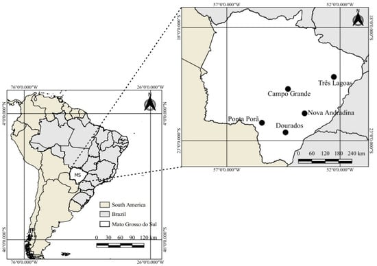
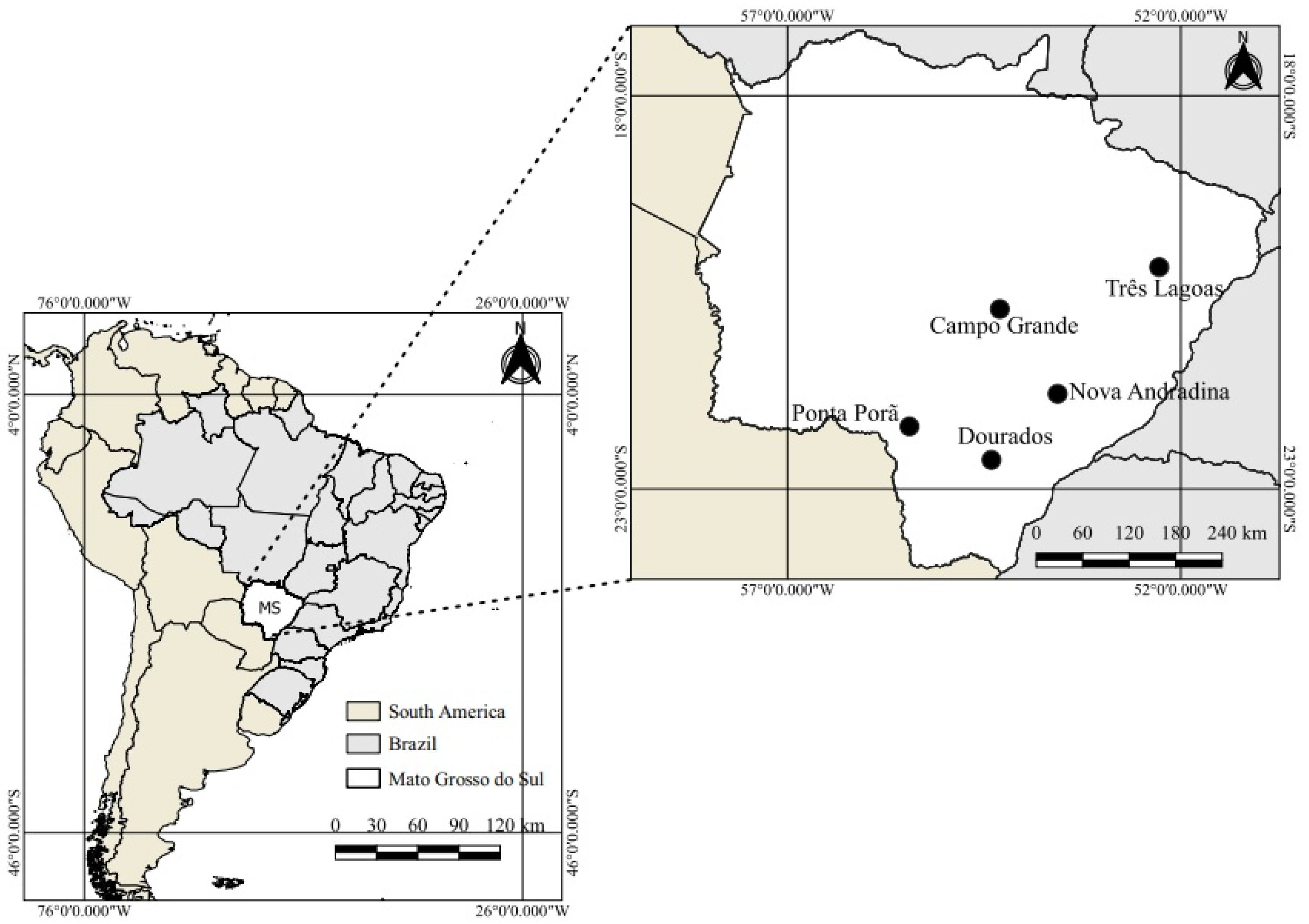
The evaluation of the PhenoGlad model was conducted under field conditions during the 2021 and 2022 growing seasons, covering five distinct locations in the state of Mato Grosso do Sul (MS), Brazil (Figure 1). The sites were selected to represent the climate variability across the state’s four mesoregions, ranging from subtropical humid (Cfa) to tropical with a dry season (Aw/Am) climates [19,20]. The municipalities and their geoclimatic characteristics are detailed in Table 1.
Figure 1.
Map of South America highlighting the state of Mato Grosso do Sul (MS) and showing the five locations used in the study (Dourados—MS, Campo Grande—MS, Três Lagoas—MS, Nova Andradina—MS, and Ponta Porã—MS).
Table 1.
Geographical coordinates and climate classification according to the Köppen system of the five experimental sites in the state of Mato Grosso do Sul, Brazil. Cfa: subtropical humid, Aw: tropical with dry winter, Am: tropical monsoon.
2.2. Plant Material and Vernalization
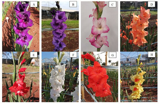
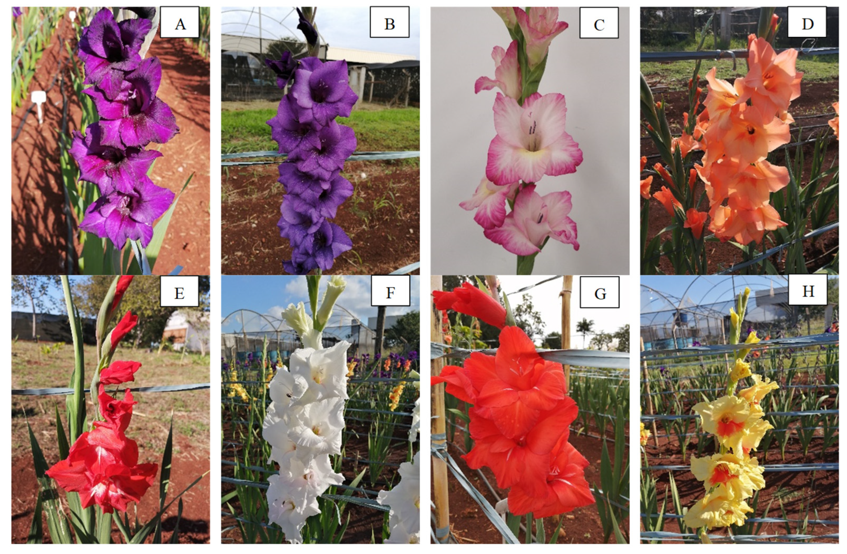
Eight commercial gladiolus (Gladiolus × grandiflorus Hort.) cultivars were used, selected based on their widespread use by farmers in Southern Brazil through the extension project “Flores para Todos” (Flowers for All). The genotypes have distinct cycles and colors (Figure 2): ‘Purple Flora’ (purple) and ‘Priscila’ (pink/cream bicolor) are classified as Early cycle; ‘Peter Pears’ (orange) and ‘Traderhorn’ (red with a white center) as Intermediate I cycle; and ‘Black Velvet’ (purple), ‘White Goddess’ (white), ‘Red Beauty’ (red), and ‘Jester’ (yellow) belong to the Intermediate II cycle. Corms with a standardized perimeter of 12–14 cm were subjected to vernalization in a cold chamber at 5 ± 1 °C for a period of 3 to 6 weeks to break dormancy and standardize sprouting. Prior to planting, the corms were acclimated for five days at 25 ± 3 °C in a protected and ventilated environment.
Figure 2.
Gladiolus cultivars used in the study: (A) Purple Flora; (B) Black Velvet; (C) Priscila; (D) Peter Pears; (E) Traderhorn; (F) White Goddess; (G) Red Beauty; and (H) Jester.
2.3. Experimental Design and Agronomic Management Practices
The experiments were conducted in a randomized complete block design (RCBD) with four replications. Each experimental plot consisted of 25 plants, totaling 100 corms per cultivar in each growing season. The experimental area was approximately 20 m2 and similar for all sites. The six central plants were used for observing the dates of developmental stages, counting the accumulated leaf number, measuring plant height, and assessing floral development. Details regarding the seasons, edaphic characteristics, and planting dates in each environment are displayed in Table 2.
Table 2.
Characterization of growing seasons, locations, soil types, cultivars, and planting dates used in the experiments in Mato Grosso do Sul. Early: Early cycle, Int: Intermediate cycle, RL: Red Latosol (Oxisol), Neosol (Entisol).
Soil preparation in all sites consisted of plowing and harrowing, with base saturation correction to 70% when necessary. Raised beds were made using a rotary bed former (1.0 m wide × 0.15 m high). Planting furrows 10 cm deep were opened in double rows (40 cm between rows). Pre-planting fertilization consisted of a broadcast application of 666 kg ha−1 of NPK 10-15-15, followed by the distribution of corms spaced at 20 cm within the row and covered with soil. At the V3 stage (third visible leaf stage), topdressing fertilization was performed with 350 kg ha−1 of urea (46% N), immediately followed by hilling up to incorporate the nitrogen and promote plant stability. At this stage, a trellising system was installed using bamboo stakes (>1.5 m) and plastic twine (raffia). Irrigation was applied via a drip system (irrigation interval of 2 days and duration of 30 min) to maintain the soil at field capacity, except in Três Lagoas, where manual irrigation was used. Weed control was performed manually, and preventive phytosanitary control was applied using products based on deltamethrin, fipronil, and Beauveria bassiana as needed.
2.4. Plant Development and Biometric Evaluations
Plant development was monitored daily at all experimental sites, following the PhenoGlad phenological scale [21]. The emergence date (VE) was defined when 50% of the sprouts became visible above the soil level [6,21]. Subsequent evaluations were performed on the six central plants marked in each plot.
During the vegetative phase, the date of appearance of each leaf (V1 to Vn) was recorded, following an alternate zigzag emission typical of the crop [14]. The accumulated leaf number (ALN) was counted weekly from V1 until complete heading (R1.2). During the reproductive phase, monitoring was conducted daily to determine the occurrence of the following key stages: beginning of heading (R1.0), complete heading (R1.2), harvest point 1 (R2—first three florets showing color), anthesis/harvest point 2 (R3), half of the flowers open (R3.4), beginning of senescence (R3.5), half of the flowers senescent (R3.6), last flower open (R4), and complete senescence (R5).
The development stage (DVS) was calculated by accumulating the daily development rate, using the following reference values according to Uhlmann et al. [6]: DVS = −1 (planting); 0 (VE); 0.8 (R1); 1.0 (R2); 1.13 (R3); 1.32 (R3.4); 1.56 (R3.5/R3.6); 1.84 (R4), and 2.0 (R5). The entire developmental cycle (from planting to R5) was evaluated in the Dourados and Ponta Porã experiments (1st and 2nd growing seasons). In the 3rd season (Dourados, Campo Grande, Três Lagoas, and Nova Andradina), development evaluation was until the commercial harvest point stage (R2), which is the main focus for cut flower producers.
2.5. Simulation and Statistical Analysis
Crop development simulations were performed using the PhenoGlad v.1.1 model [6], freely available at http://coral.ufsm.br/phenoglad/ (accessed on 25 January 2021). The model inputs included maximum and minimum air temperatures, planting date, and the cultivar or maturity cycle.
Daily meteorological data were obtained from automatic weather stations located near the experimental sites. In Dourados, data were used from the Embrapa Agropecuária Oeste station (15 km distance) and the UFGD station (6.5 km; starting on 28 April 2021), available on the Guia Clima platform. For Campo Grande and Três Lagoas, stations A702 (at 5 km) and A704 (at 700 m) from the National Institute of Meteorology (INMET) were used, respectively. In Ponta Porã, data came from the INMET A703 station (at 14 km) and from the Centro de Monitoramento do Tempo e do Clima do Estado de Mato Grosso do Sul (CEMTEC). For Nova Andradina, the INMET S713 station (at 1 km) and CEMTEC data were used.
For cultivars that were not available in the PhenoGlad model (‘Black Velvet’, ‘Red Beauty’, ‘Priscila’, and ‘Traderhorn’), simulations used the corresponding maturity-cycle class (Early or Intermediate) according to Uhlmann et al. [6]. This procedure follows the original model calibration, preserves the developmental thermal-time structure, and does not affect cultivar-level comparisons within the model framework.
The evaluation of the PhenoGlad model consisted of comparing the field-observed data (Obs) and the model-simulated data (Sim) for the occurrence of developmental stages and the accumulated leaf number (ALN), a key biological indicator because leaf appearance follows a predictable pattern in gladiolus and reflects the crop’s thermal response. Model performance was quantified using the following statistics:
Root mean square error (RMSE): evaluates the average magnitude of the error [22].
BIAS index: measures the tendency to under- or overestimate [23].
Correlation coefficient (r): indicates the degree of linear association [24].
Willmott’s index of agreement (d): measures the overall accuracy, ranging from 0 to 1 [24].
where
- Si = Simulated values;
- S = Mean of simulated values;
- Oi = Observed values;
- = Mean of observed values;
- n = Number of observations.
Model performance was interpreted based on low RMSE values, BIAS close to zero, and higher values of Willmott’s index of agreement (d), with d values above 0.90 indicating very good agreement between the observed and simulated data.
2.6. Climate Risk Simulation (Cold and Heat)
The quantification of risks due to abiotic stress was based on the alerts issued by the PhenoGlad algorithm [6]:
Heat damage: considered when the maximum temperature (Tmax) ≥ 34 °C for three consecutive days during the reproductive phase (R1 to R5). If the simulation goes up to R2, the alert indicates a risk of severe sepal “burning”. If it goes up to R5, this indicates a risk of the last 3–4 spike florets failing to open.
Cold damage: considered when the minimum temperature (Tmin) ≤ −2 °C on a single day (severe frost) or when Tmin ranges between −2 °C and 3 °C for three consecutive days starting from emergence (VE). Such conditions indicate a risk of spike damage or leaf yellowing.
3. Results
3.1. Meteorological Conditions and Emergence
Mean air temperatures during the experimental periods ranged from 19.3 °C (Dourados, Season 3) to 24.1 °C (Três Lagoas), as detailed in Table 3. The absolute minimum temperature was 11.7 °C during the winter in Dourados, while the mean maximum temperature exceeded 31 °C in Três Lagoas and in the second season in Dourados. The accumulated rainfall ranged from 247.6 mm (Campo Grande) to 429.4 mm (Ponta Porã), with the exception of Três Lagoas, which recorded only 38.0 mm during the cycle.
Table 3.
Summary of meteorological variables (mean minimum(Min), average(Avg), and maximum(Max) air temperatures, accumulated rainfall(Prec.), and mean relative humidity(RH)) during the experiments conducted in different municipalities in the state of Mato Grosso do Sul for evaluating the PhenoGlad simulation model.
Regarding developmental phases, the duration from planting to emergence (VE) varied from 6 to 22 days across the different seasons and cultivars. In Dourados (Seasons 1 and 2), the emergence of most cultivars (‘Purple Flora’, ‘Peter Pears’, ‘Black Velvet’) occurred between 10 and 12 days after planting (DAP), while the cultivar ‘Jester’ emerged at 18 DAP in both seasons. The shortest period for emergence was recorded in the cultivar ‘Priscila’ (6 days) and the longest in ‘Red Beauty’ (22 days), both in the third growing season in Dourados. In the other locations (Campo Grande, Três Lagoas, Nova Andradina, and Ponta Porã), the time until emergence ranged between 8 and 14 days for the evaluated cultivars (‘Purple Flora’, ‘Jester’, ‘Peter Pears’, and ‘White Goddess’).
3.2. Model Performance in Dourados: Simulations Starting from Planting and from Emergence
The accuracy of the PhenoGlad model in simulating the accumulated leaf number (ALN) and the days to reach developmental stages (DAP/DAE) showed high agreement with the observed data across the three growing seasons in Dourados. The index of agreement (d) and the correlation coefficient (r) remained consistently high, ranging from 0.98 to 1.00 for different planting dates and cultivars. The BIAS index oscillated around zero (from −0.27 to +0.32), indicating no tendency for the model to under- or overestimate (Figure A1, Figure A2, Figure A3, Figure A4, Figure A5 and Figure A6—Appendix A).
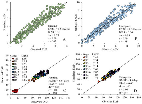
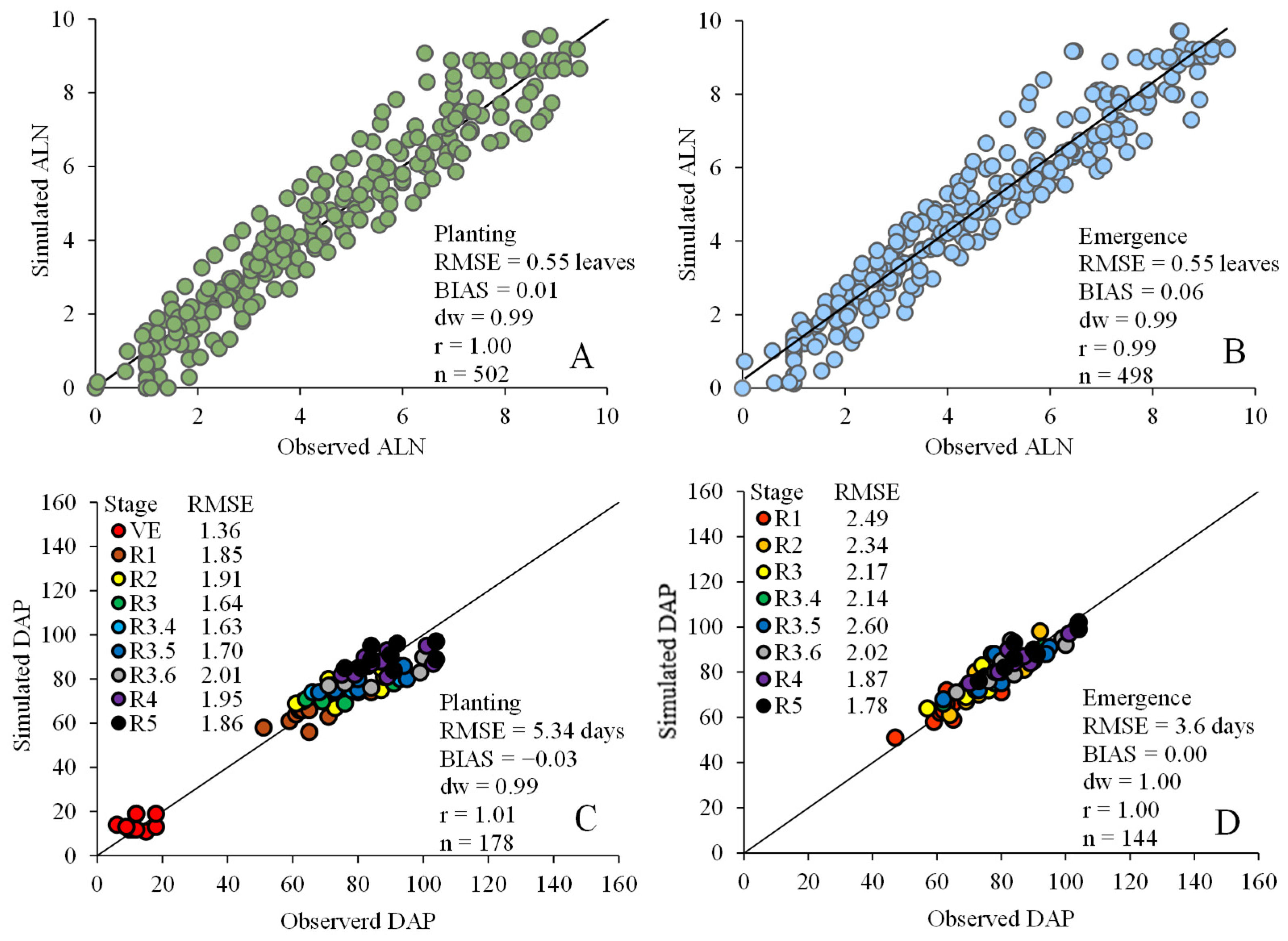
In the analyses arranged by growing season, the RMSE for ALN ranged from 0.12 to 0.76 leaves when the model was initiated at the planting date (PL), and from 0.09 to 0.95 leaves when initiated at the emergence date (VE). Pooling the data from all cultivars and the three growing seasons in Dourados (Figure 3), the overall RMSE for ALN was identical in both simulation methods (0.55 leaves). The BIAS for ALN was +0.01 (PL) and +0.06 (VE).
Figure 3.
Simulated versus observed accumulated leaf number (ALN) when starting the simulation with the PhenoGlad model at planting (A) and at emergence (B); and simulated versus observed number of days to developmental stages starting from planting (C) and from emergence (D). Data are pooled for the three growing seasons in Dourados/MS and for eight gladiolus cultivars (‘Purple Flora’, ‘Black Velvet’, ‘Peter Pears’, ‘White Goddess’, ‘Jester’, ‘Priscila’, ‘Traderhorn’, and ‘Red Beauty’). Simulated and observed developmental stages: emergence (VE), beginning of heading (R1.0), complete heading (R1.2), harvest point 1 (R2), anthesis/harvest point 2 (R3), half of the flowers open (R3.4), beginning of senescence (R3.5), half of the flowers senesced (R3.6), last flower open (R4), and complete senescence (R5). The solid line represents the 1:1 line. RMSE = root mean square error, BIAS = bias index, dw = index of agreement, r = correlation coefficient; n = number of observations.
For estimating the number of days to achieve each of the developmental stages, seasonal analyses showed RMSE ranging from 0.65 to 3.40 days for simulations when the model started at PL, and from 0.44 to 3.68 days when the model started at VE, with variations depending on the cultivar. The cultivar ‘Peter Pears’ tended to have the lowest errors (e.g., 0.44 days in the second growing season when starting the simulation at VE), while ‘Jester’ and ‘White Goddess’ had the highest error.
The analysis pooling the developmental data from the three seasons (Figure 3) revealed a substantial difference in overall model performance depending on the starting point of the simulation. The simulation initiated from planting (PL) resulted in a pooled RMSE of 5.34 days. In contrast, when the simulation was initiated from the emergence date (VE), the pooled RMSE was reduced to 3.16 days. The pooled BIAS for phenology remained low, at −0.03 for PL and 0.00 for VE.
3.3. Multilocation Evaluation of the PhenoGlad Model
The model performance was also satisfactory when evaluated in the other municipalities, covering different edaphoclimatic conditions in Mato Grosso do Sul, with variations in accuracy depending on the simulation (starting from planting (PL) or emergence (VE)).
In the Campo Grande environment (Figure A7), the simulation initiated from emergence (VE) resulted in high accuracy for phenology and leaf appearance. For the ‘Purple Flora’ cultivar, the RMSE for the development stages (DVS) was only 0.77 days, and 0.21 leaves for ALN. For the ‘White Goddess’ cultivar, the model was highly accurate in predicting the most important stage for growers (R2—harvest point), showing an error of only 0.94 days, and an RMSE of 0.65 leaves for ALN when simulated from VE.
In Três Lagoas (Figure A8), regarding the model performance for ‘Purple Flora’, the RMSE of the DVS was identical (1.18 days) when the simulations started at PL and at VE. However, the ALN error was lower when simulation started at planting (0.98 leaves). For the ‘Jester’ cultivar, the simulation from emergence showed a lower error for leaf appearance (0.73 leaves), but with a higher error for the reproductive stages (6.71 days). The simulation started from planting was more accurate for the reproductive stages in the ‘Jester’ cultivar.
In Nova Andradina (Figure A9), simulation errors were consistently low. For the ‘Purple Flora’ cultivar, the highest model accuracy occurred with the simulation starting at PL (RMSE of 0.38 days), while the best accuracy for ALN was obtained when starting simulations at VE (0.24 leaves). A similar response occurred for the ‘Peter Pears’ cultivar, whose lowest error was recorded when starting at VE (0.45 days), with an error in ALN in the range of 0.25 leaves.
Finally, in Ponta Porã (Figure A10), the pattern of high accuracy was repeated. For the ‘Purple Flora’ cultivar, the lowest error for DVS (0.72 days) and ALN (0.27 leaves) was obtained in simulations starting from emergence. For the ‘Peter Pears’ cultivar, simulation from VE was also superior for developmental stages (RMSE of 0.62 days), although the simulation of leaf appearance showed a lower error when initiated from planting (0.41 leaves).
Although simulations initiated from emergence (VE) generally showed higher accuracy, this pattern was not uniform across all cultivars and environments. In Três Lagoas, Nova Andradina, and Ponta Porã, simulations starting from planting (PL) occasionally produced similar or lower errors for specific traits such as ALN or reproductive development, highlighting that the relative performance of VE and PL depends on cultivar-specific and environmental interactions.
3.4. Prediction of Climate Risks and Observed Damage
The PhenoGlad model’s alert system did not identify any risk of low-temperature damage during the experiments (Tmin < 3 °C for three consecutive days or < −2 °C on a single day), which was corroborated by the absence of cold injury symptoms in the field. Conversely, when simulated from planting, the model issued multiple alerts for high-temperature stress during the reproductive phase, a condition triggered when the maximum daily temperature reaches or exceeds 34 °C for three consecutive days [6].
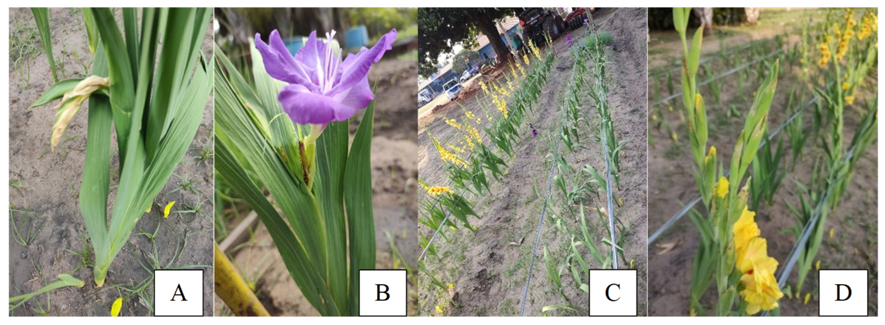
In the experiment at Três Lagoas, the model accurately warned of the risk of severe damage to the flowers before the harvest point and the failure of the last florets to open. For the ‘Purple Flora’ cultivar, the first alert was issued on Day of the Year (DOY) 240 (28 August), triggered by the thermal sequence of 35.0 °C, 35.8 °C, and 37.2 °C. A second alert occurred on DOY 252 (9 September) following an even more extreme thermal sequence of 34.1 °C, 37.9 °C, and 40.1 °C. For the ‘Jester’ cultivar, the alert was also issued on DOY 252. These predictions were fully confirmed by field evaluations, where severe visible damage was observed, such as burning, wilting of developing floral spikes, and poor stem formation (Figure 4).
Figure 4.
Visible damage caused by heat stress (high temperatures) during the reproductive phase in Três Lagoas/MS: (A) burning and wilting of the spike of the ‘Purple Flora’ cultivar at the beginning of heading; (B) structural malformation of the floral stem in the ‘Purple Flora’ cultivar; (C) genotype difference, with the ‘Jester’ cultivar flowering and the ‘Purple Flora’ cultivar showing reproductive inhibition (absence of flowers); (D) leaves and flowers damaged in the ‘Jester’ cultivar.
In Dourados (second season), the model also warned of thermal damage risks. For the ‘Purple Flora’ cultivar, the alert occurred on DOY 272 (29 September), triggered by the sequence of 36.1 °C, 37.9 °C, and 37.5 °C. For the ‘Peter Pears’ cultivar, the alert was generated on DOY 273 (30 September), with consecutive maximum temperatures of 37.9 °C, 37.5 °C, and 38.5 °C. While direct petal burning was not observed in ‘Peter Pears’ in the field, heat stress exerted a drastic physiological impact on the ‘Purple Flora’ cultivar: reproductive development was severely inhibited by the high temperatures, resulting in only two plants (2% of a 100-corm stand) reaching heading. The heat stress alerts issued by the model in Três Lagoas fully corresponded to the severe field damage observed. In Dourados (second season), the alert for ‘Purple Flora’ also matched the damage pattern, whereas the alert for ‘Peter Pears’ did not result in visible injury, representing a false-positive event. In all other municipalities, no alerts were issued and no heat-related damage occurred, indicating the absence of false-negative events in the multilocation evaluation.
4. Discussion
4.1. Genetic–Environmental Dynamics and the Physiology of Emergence
The exposure of gladiolus plants to multiple combinations of planting dates, locations, and soil types in this study provides a rich data set for testing the predictive robustness of the PhenoGlad model. The detailed analysis of the emergence phase demonstrated that the sprouting rate is not static but rather responds intensely to the complex interaction between the genotype and the environmental conditions of each growing period, corroborating with recent findings in the literature [13,16,25,26]. This became evident when observing that, under the same mean temperature of 19.25 °C during the winter in Dourados, the ‘Priscila’ cultivar (Early cycle) emerged rapidly in just 6 days, while ‘Red Beauty’ (Intermediate II cycle) required 22 days for initial establishment. This wide range of duration in the sprouting phase (PL-EM) may be related to the physiology of corm dormancy. In the present study, all cultivars of corms were subjected to cold no-freezing treatment (vernalization), which is widely recommended and used to increase sprouting rates and break dormancy in gladiolus corms and other species [27]. However, the fact that they were grown under identical conditions and still exhibited such discrepant emergence times suggests that the intrinsic physiological barriers of each genotype outweighed the isolated effect of vernalization.
Dormancy in gladiolus can last from two to four months and has been associated with the accumulation of endogenous growth inhibitors, including abscisic acid (ABA) [28,29,30]. Although ABA plays an important role in this process, dormancy regulation is known to involve multiple hormonal and metabolic pathways. In this context, the variation observed among cultivars in the duration of the sprouting phase is consistent with genotype-specific differences in dormancy release requirements, rather than the action of a single regulatory mechanism.
In addition to genetics, microclimatic conditions played a key role in the initial development rate. The constancy of some cultivars, such as ‘Jester’, which maintained an emergence time of 18 days across different planting seasons in Dourados, strongly contrasted with the plasticity observed in ‘Purple Flora’ and ‘Peter Pears’, whose times fluctuated significantly in the other locations (Campo Grande, Três Lagoas, Nova Andradina, and Ponta Porã). From an agronomic standpoint, this variability highlights a strong genotype × environment interaction. The implications of these results for extensionists, consultants, and growers is that the choice of cultivars must consider not only the aesthetics and visual appeal of different cultivars but also the adaptability and stability of each cultivar to local edaphoclimatic conditions, thereby optimizing the initial crop stand and maximizing productive efficiency.
4.2. Mathematical Coupling: The Higher Accuracy of Simulation Starting from Emergence
From a modeling perspective, the present study stands out as a pioneer in the Midwest region of Brazil. The integrated analysis showed that shifting the initial simulation trigger to VE substantially increases the predictive accuracy of the PhenoGlad model. By pooling the three seasons in Dourados, the RMSE for predicting phenological development stages experienced a significant reduction, dropping from 5.34 days (when initiated at PL) to 3.16 days (when initiated at VE).
In the multilocation trials (Campo Grande and Ponta Porã), the simulation from emergence maintained this pattern of higher accuracy. Some exceptions—such as the variation in Três Lagoas (where the ‘Jester’ cultivar had lower accuracy in VE) and in Nova Andradina (where ‘Purple Flora’ performed better in PL for phenology, but ‘Peter Pears’ performed better in VE)— reinforce the complexity of the genotype × environment interaction. This observation is consistent with previous studies [6,7], which also recommend initiating the simulation from crop emergence, since the belowground phase is driven by a complex of variables not taken into account in the PhenoGlad model, such as soil moisture, micrometeorological variations, planting depth, and corm dormancy.
The magnitude of the error in predicting the developmental stages starting the simulation at crop emergence (RMSE of 3.16 days) confirms that the PhenoGlad model performs excellently for the state of Mato Grosso do Sul, as this error is lower than the RMSE reported in the subtropics of Southern Brazil (6.9 days in Santa Catarina [13] and 4.3 to 5.2 days in Rio Grande do Sul [6], approaching the very high performance of 2.08 days reported in Paraná [14]. Besides its applicability in temperate and subtropical environments, maintaining its predictive capacity at around three days in the tropics corroborates the robustness of PhenoGlad, as also attested in recent validations under high temperature climates, such as in the semiarid region of Northeastern Brazil [16] and in extreme subtropical conditions in Punjab, India [15]. These results reinforce the value of regional-scale process-based modeling as a practical framework for extending calibrated crop models to new environments without substantial loss of predictive performance [8].
It is important to note, however, that VE was not universally superior across all cases. The scenarios in Três Lagoas, Nova Andradina, and Ponta Porã, where PL performed equally well or even better for certain developmental traits, reflect meaningful genotype × environment interactions. These exceptions reinforce that the advantage of initiating simulations at VE is context-dependent and that both starting points can provide valuable information depending on cultivar behavior and local conditions.
In the context of agricultural engineering and for practical application, a predictive error of about five days is acceptable. The market demand for gladiolus is highly concentrated on peak dates such as Mother’s Day and All Souls’ Day. If the model underestimates the harvest, simulating the harvest point (R2) up to five days before the commercialization target, the grower has the technical viability to store the stems in cold storage (5 to 8 °C) for up to 15 days. This practice delays the progress of floral opening, preserving aesthetic quality and ensuring product availability, which is vital for securing family income [6,13].
Regarding leaf development, the model simulated the accumulated leaf number (ALN) with high precision. Across all seven seasons and locations evaluated, the RMSE for ALN remained consistently below one leaf, which is excellent for practical application in gladiolus [6]. Similar performance of the PhenoGlad model was also reported in Paraná (0.54 leaves [13]) and in Rio Grande do Sul and Santa Catarina, with RMSE values ranging from 0.4 to 0.8 leaves across eight cultivars [6].
The results presented in this study with robust statistical indices—with Pearson’s correlation coefficient (r) and the index of agreement (d) greater than 0.98 for all cultivars and regions studied—indicate that the PhenoGlad model is, not only as a mathematical algorithm but also as a technological advancement, applicable to floriculture in the state of Mato Grosso do Sul. These results demonstrate that extension agents, consultants, and growers can use the model as a powerful tool to optimize planting dates, maximize flower quality, and mitigate climatic risks.
4.3. Ecophysiology Under Thermo-Hydric Extremes in a Transition Climate
The growth, development, and floral stem quality of gladiolus are driven by temperature [4,6,21]. Gladiolus crops have optimal development temperatures of 28 °C for the vegetative phase and 25 °C for the reproductive phase [3]. Deviations of the daily temperature from these optimal values trigger non-linear biological responses. When the temperature exceeds this optimal level, the development rate decreases in the model, resulting in a longer developmental cycle and exposing the plant to physiological stress [6,31].
The extrapolation of the crop to the transition region of the Mato Grosso do Sul Cerrado highlighted these limitations in practice. Among all the municipalities evaluated, the experiment conducted in Três Lagoas (winter/spring) stood out due to the occurrence of heat stress with visible damage in the field, observed by the growers and predicted by the PhenoGlad model alerts. This reproductive collapse was not solely the result of absolute maximum temperatures exceeding 34 °C for three consecutive days, but rather a destructive synergistic environmental interaction: high temperatures associated with low relative air humidity. A mean relative humidity (MRH) of only 59% was recorded at the site, a condition considerably lower than the ideal range of 60% to 70% required by the crop [32].
Previous studies support the severity of combined heat and atmospheric drought stress in gladiolus. High temperature can impair floral development and quality in gladiolus, while high atmospheric evaporative demand intensifies plant water loss and physiological stress [4,5,33]. In Três Lagoas, the combination of dry and hot air generated a high evapotranspirative demand that possibly depleted plant turgor and accelerated senescence. This atmospheric water deficit, uncompensated by irrigation, compromised the final development and rendered the most sensitive cultivars, such as ‘Purple Flora’, commercially unviable.
From an ecophysiological perspective, the simultaneous exposure to high temperatures and low relative humidity substantially increases the vapor pressure deficit (VPD), intensifying transpiration demand while reducing stomatal conductance. Under elevated VPD, plants face hydraulic and metabolic constraints that accelerate leaf water loss, impair carbon assimilation, and reduce their capacity to sustain reproductive development—a set of responses widely documented under atmospheric drought and elevated vapor pressure deficit conditions [33,34,35]. This framework is consistent with the symptoms observed in Três Lagoas, where the combination of hot and dry air likely exceeded the hydraulic buffering capacity of gladiolus, culminating in floral spike collapse, floret abortion, and the complete reproductive failure of sensitive cultivars such as ‘Purple Flora’.
The agreement between predicted alerts and observed damage was high, particularly in Três Lagoas and in the case of ‘Purple Flora’ in Dourados. A single false-positive event occurred for ‘Peter Pears’, which showed no visible injury despite an alert. Importantly, no false-negative events were detected across the multilocation experiments, indicating that the model did not fail to identify any damaging heat stress episodes.
Faced with the reality of these seasonal climatic challenges in the Midwest of Brazil—where temperatures frequently exceed 35 °C—the adoption of management strategies and adaptive agricultural engineering measures is crucial [2,3]. A viable alternative to maintain the commercial quality of the floral stems is the implementation of thermo-reflective shade nets [5,7]. Although gladiolus benefits from adequate solar radiation for full growth and development, shading acts by protecting the inflorescences during peak thermal stress, enabling constant annual production [5,7,32]. In this scenario of climate adaptation, the use of the PhenoGlad model adds substantial technological value, as it allows the prediction of exactly which time windows require investment in these nets to prevent crop failure.
4.4. Water Deficit and the Inhibition of Reproductive Differentiation
The analysis of crop development dynamics under climate transition conditions requires, in addition to temperature, an understanding of the water balance in the soil–plant–atmosphere system. Accumulated rainfall varied drastically among locations. While the second planting season in Dourados was supplied with 361.4 mm of rain, environments like Três Lagoas recorded only 38.0 mm, and in Nova Andradina, rainfall was zero during the evaluated period. Under these conditions of rainfall restriction, the adoption of irrigation (drip or manual) was obligatory. However, the interaction with the high atmospheric evaporative demand revealed the physiological limits of the crop, suggesting that, under extreme vapor pressure deficit, root absorption was possibly unable to compensate for leaf water loss.
Although water excess promotes corm rot, recent studies indicate that the greatest vulnerability of gladiolus lies in water deficit, specifically during vegetative growth [36,37,38]. The classic symptoms of this stress—reduction in foliar development, cycle delay, stunting, and loss of aesthetic quality—may intensify under prolonged water restriction [36,38,39]. Water restriction, particularly if extended until heading, may severely compromise reproductive development, leading to dehydration and, in severe cases, inflorescence abortion [36,37,38].
The extreme reproductive collapse observed in this study, where plants remained in the vegetative phase without producing floral stems, is justified by the ecophysiology of apical differentiation [40]. The formation of the meristem that will differentiate into the flower stem does not occur late but rather in a very early and specific window, at the V3 stage [15]. Mazzini-Guedes et al. [37] corroborates this dynamic by demonstrating that gladiolus cultivation maintained at 80% of field capacity results in long, high-aesthetic-standard stems. In contrast, when the soil reaches water depletion (25% of field capacity), the plants do not even differentiate floral stems, which may explain the failures observed in Três Lagoas—a premise validated by recent research attesting to the commercial unviability of stems subjected to suboptimal irrigation depths [36,37,38].
Therefore, from the perspective of biosystem engineering, it is inferred that the volume of irrigation provided, although sufficient for vegetative survival, was possibly unable to maintain the soil at optimal field capacity. The high temperatures combined with low relative air humidity suggest there was an evapotranspirative demand greater than the rate of root absorption. It is likely that an acute water deficit at the V3 stage acted as the primary limiting abiotic factor, physiologically inhibiting heading. Such a hypothesis indicates that, in environments with high evaporative demand, the use of simulation models like PhenoGlad can benefit from adequate water dimensioning to support floriculture in the Cerrado.
5. Conclusions
The PhenoGlad model demonstrated high predictive accuracy in simulating the developmental stages and accumulated leaf number of gladiolus cultivars across multiple environments and planting dates in Mato Grosso do Sul, Brazil. Starting simulations from crop emergence substantially reduced prediction errors and improved the representation of developmental timing under tropical-transition conditions.
The model also successfully predicted heat stress damage, accurately issuing alerts for high-temperature sequences that later resulted in reproductive inhibition and floral injury in the field. Therefore, PhenoGlad fulfills the objective of this study and is an appropriate decision-support tool for floriculture in emerging agricultural frontiers. Its application supports strategic scheduling of planting dates, anticipation and mitigation of thermal risks, and improved environmental management in tropical environments.
Author Contributions
Conceptualization, P.M.S.F., J.C.S., D.B., L.O.U., and N.A.S.; methodology, P.M.S.F., J.C.S., R.T., D.B., L.O.U., and N.A.S.; software, P.M.S.F., J.C.S., J.C.M.R., L.C.R., L.M.R., R.T., and L.O.U.; validation, P.M.S.F., J.C.S., J.C.M.R., L.C.R., M.R.R., and M.A.D.; formal analysis, P.M.S.F., J.C.M.R., L.C.R., L.M.R., R.T., and L.O.U.; investigation, P.M.S.F., J.C.M.R., L.C.R., L.M.R., M.R.R., and M.A.D.; resources, J.C.S. and N.A.S.; data curation, P.M.S.F., J.C.M.R., M.R.R., M.A.D., and L.O.U.; writing—original draft preparation, P.M.S.F., J.C.S., and L.O.U.; writing—review and editing, J.C.S., L.M.R., and N.A.S.; visualization, P.M.S.F., J.C.S., and N.A.S.; supervision, J.C.S., L.O.U., and N.A.S.; project administration, P.M.S.F. and J.C.S.; funding acquisition, J.C.S. All authors have read and agreed to the published version of the manuscript.
Funding
This research was funded by the National Council for Scientific and Technological Development (CNPq, Proc. No. 308942/2020-5) and by the Coordination for the Improvement of Higher Education Personnel (CAPES), Finance Code 001, through scholarship support.
Institutional Review Board Statement
Not applicable.
Informed Consent Statement
Not applicable.
Data Availability Statement
The raw data supporting the conclusions of this article will be made available by the authors on request.
Acknowledgments
The authors acknowledge the research support provided by the Federal University of Grande Dourados (UFGD), the Research and Extension Group in Ornamental Horticulture (GEHORTI-UFGD), the PhenoGlad team at the Federal University of Santa Maria (UFSM), the Federal Institute of Mato Grosso do Sul (IFMS), Nova Andradina Campus and Ponta Porã Campus, and biologist Flavio Henrique Fardin for his support in the research conducted in Três Lagoas.
Conflicts of Interest
The authors declare no conflicts of interest.
Abbreviations
The following abbreviations are used in this manuscript:
| ALN | Accumulated leaf number |
| RMSE | Root mean square error |
| BIAS | Bias index |
| r | Correlation coefficient |
| d | Willmott’s index of agreement |
| DVS | Development stage |
| DAP | Days after planting |
| DAE | Days after emergence |
| VE | Emergence |
| PL | Planting |
| DOY | Day of the Year |
| Tmax | Maximum temperature |
| Tmin | Minimum temperature |
| RCBD | Randomized complete block design |
| NPK | Nitrogen, Phosphorus, Potassium |
Appendix A
Figure A1.
Simulation from planting date (first season, Dourados/MS). Simulated versus observed accumulated leaf number (ALN) for the cultivars ‘Purple Flora’ (A), ‘Black Velvet’ (C), ‘Peter Pears’ (E), ‘White Goddess’ (G), and ‘Jester’ (I). Simulated versus observed days after planting (DAP) to reach phenological stages in the respective cultivars (B,D,F,H,J). Evaluated stages: beginning of heading (R1.0), complete heading (R1.2), harvest point 1 (R2), harvest point 2/anthesis (R3), half of the florets open (R3.4), beginning of senescence (R3.5), half of the florets senescent (R3.6), last floret open (R4), and total senescence (R5). The solid line represents the 1:1 ratio. The inset graphs represent the dispersion of residuals. RMSE = root mean square error; BIAS = bias index; dw = index of agreement; r = correlation coefficient; n = number of observations.
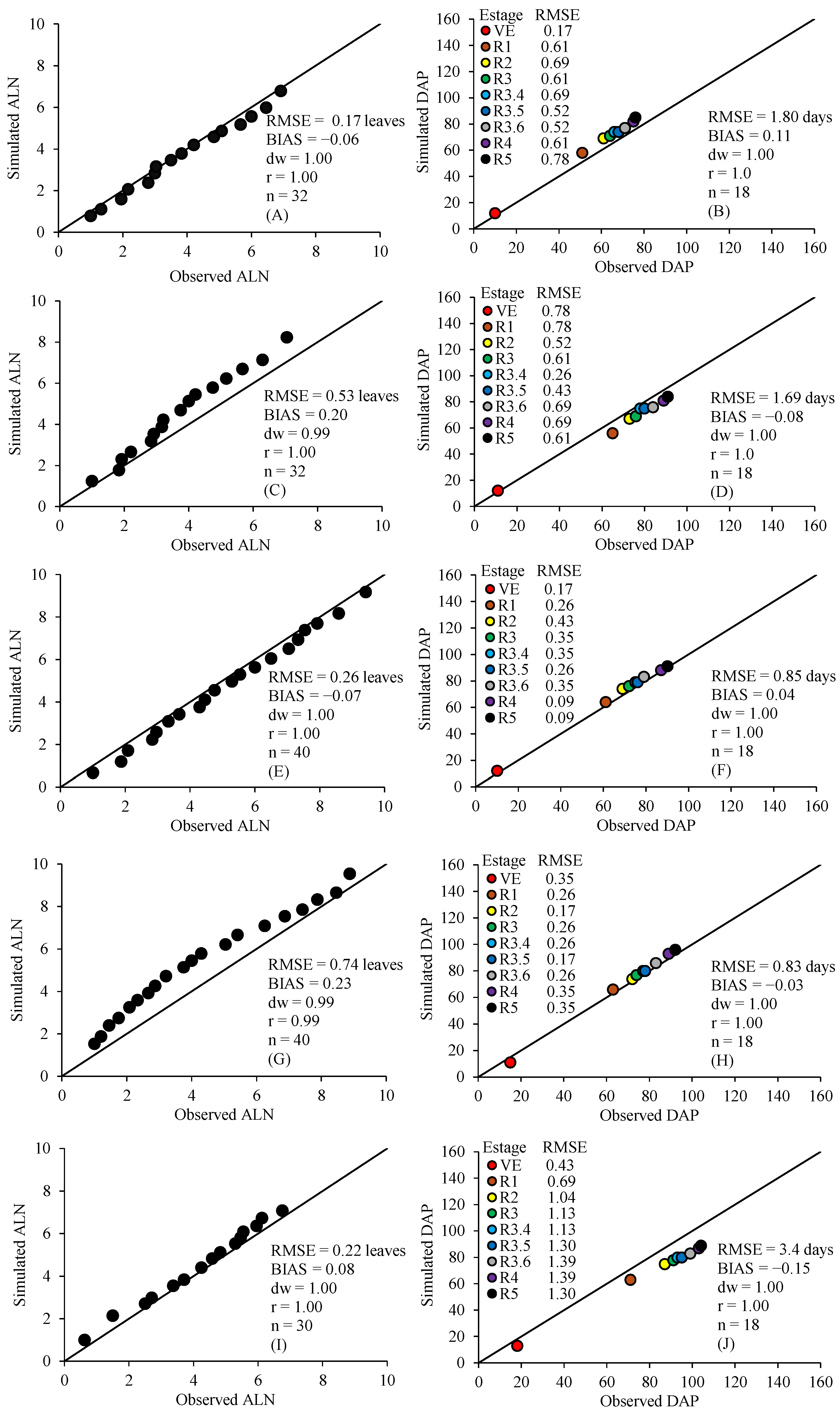
Figure A2.
Simulation from emergence date (first season, Dourados/MS). Simulated versus observed accumulated leaf number (ALN) for the cultivars ‘Purple Flora’ (A), ‘Black Velvet’ (C), ‘Peter Pears’ (E), ‘White Goddess’ (G), and ‘Jester’ (I). Simulated versus observed days after emergence (DAE) to reach phenological stages (R1.0 to R5) in the respective cultivars (B,D,F,H,J). The solid line represents the 1:1 ratio. The inset graphs represent the dispersion of residuals. RMSE = root mean square error; BIAS = bias index; dw = index of agreement; r = correlation coefficient; n = number of observations.
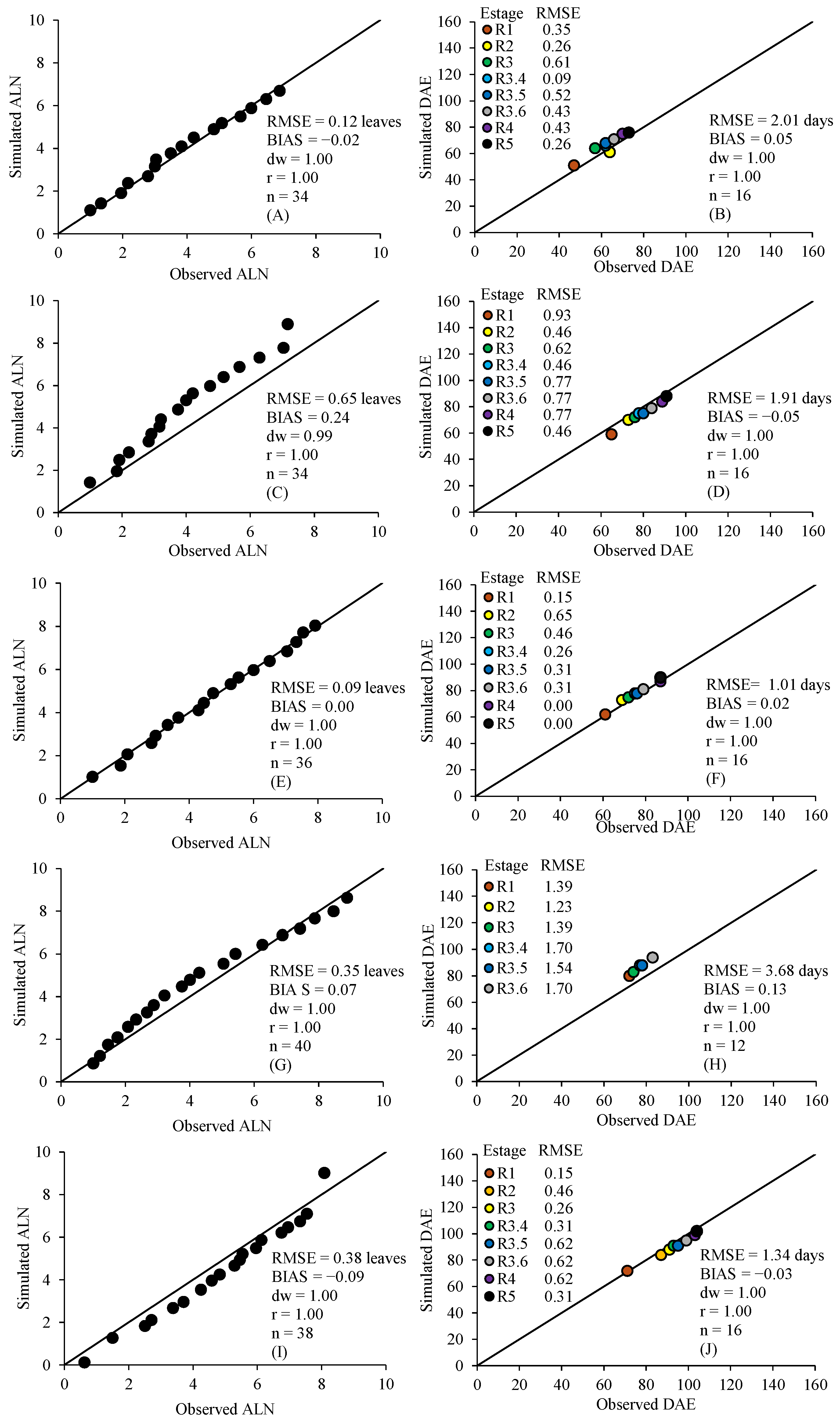
Figure A3.
Simulation from planting date (second season, Dourados/MS). Simulated versus observed accumulated leaf number (ALN) for the cultivars ‘Purple Flora’ (A), ‘Peter Pears’ (C), ‘White Goddess’ (E), and ‘Jester’ (G). Simulated versus observed days after planting (DAP) to reach phenological stages (R1.0 to R5) in the respective cultivars (B,D,F,H). The solid line represents the 1:1 ratio. The inset graphs represent the dispersion of residuals. RMSE = root mean square error; BIAS = bias index; dw = index of agreement; r = correlation coefficient; n = number of observations.
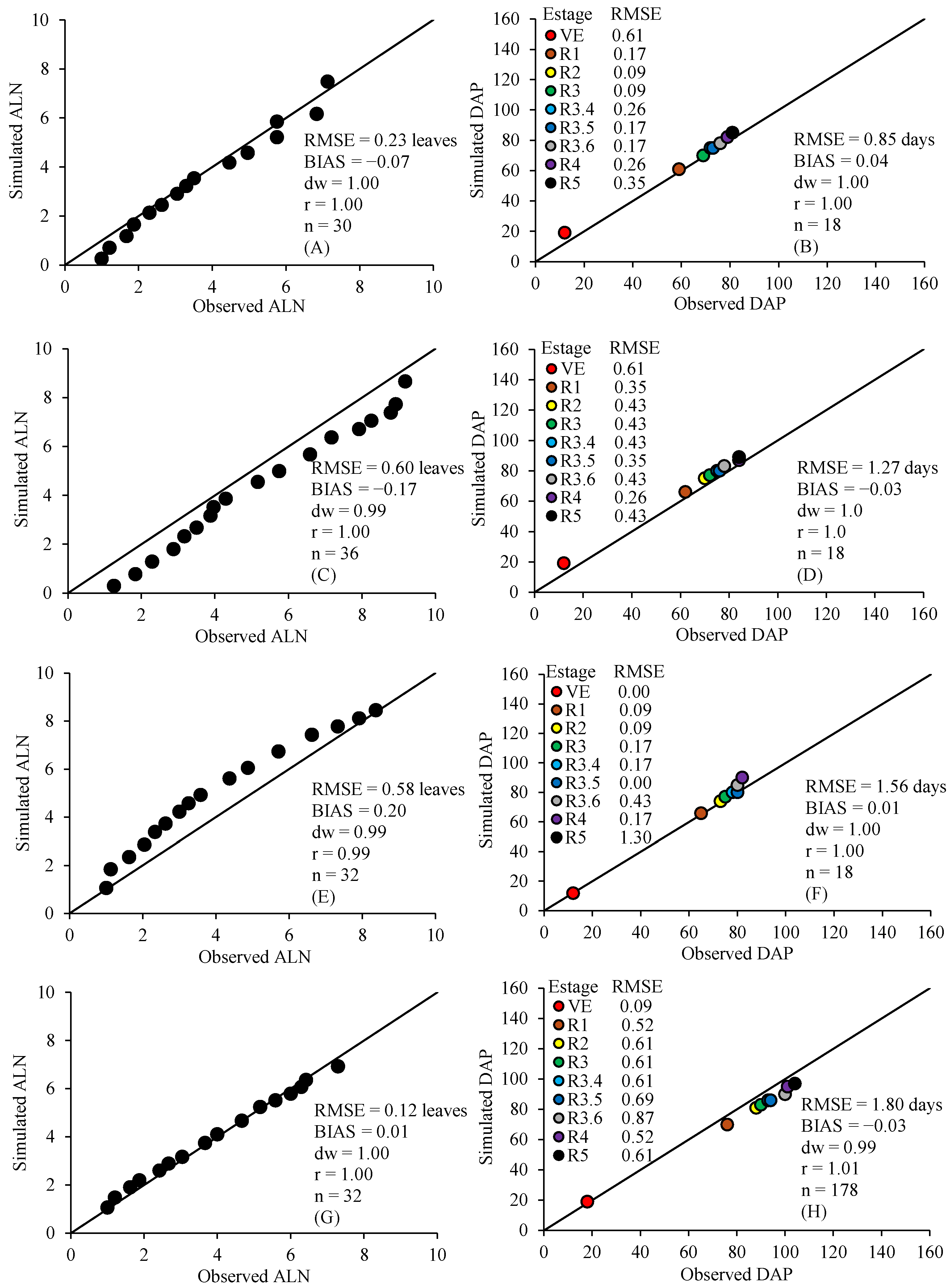
Figure A4.
Simulation from emergence date (second season, Dourados/MS). Simulated versus observed accumulated leaf number (ALN) for the cultivars ‘Purple Flora’ (A), ‘Peter Pears’ (C), ‘White Goddess’ (E), and ‘Jester’ (G). Simulated versus observed days after emergence (DAE) to reach phenological stages (R1.0 to R5) in the respective cultivars (B,D,F,H). The solid line represents the 1:1 ratio. The inset graphs represent the dispersion of residuals. RMSE = root mean square error; BIAS = bias index; dw = index of agreement; r = correlation coefficient; n = number of observations.
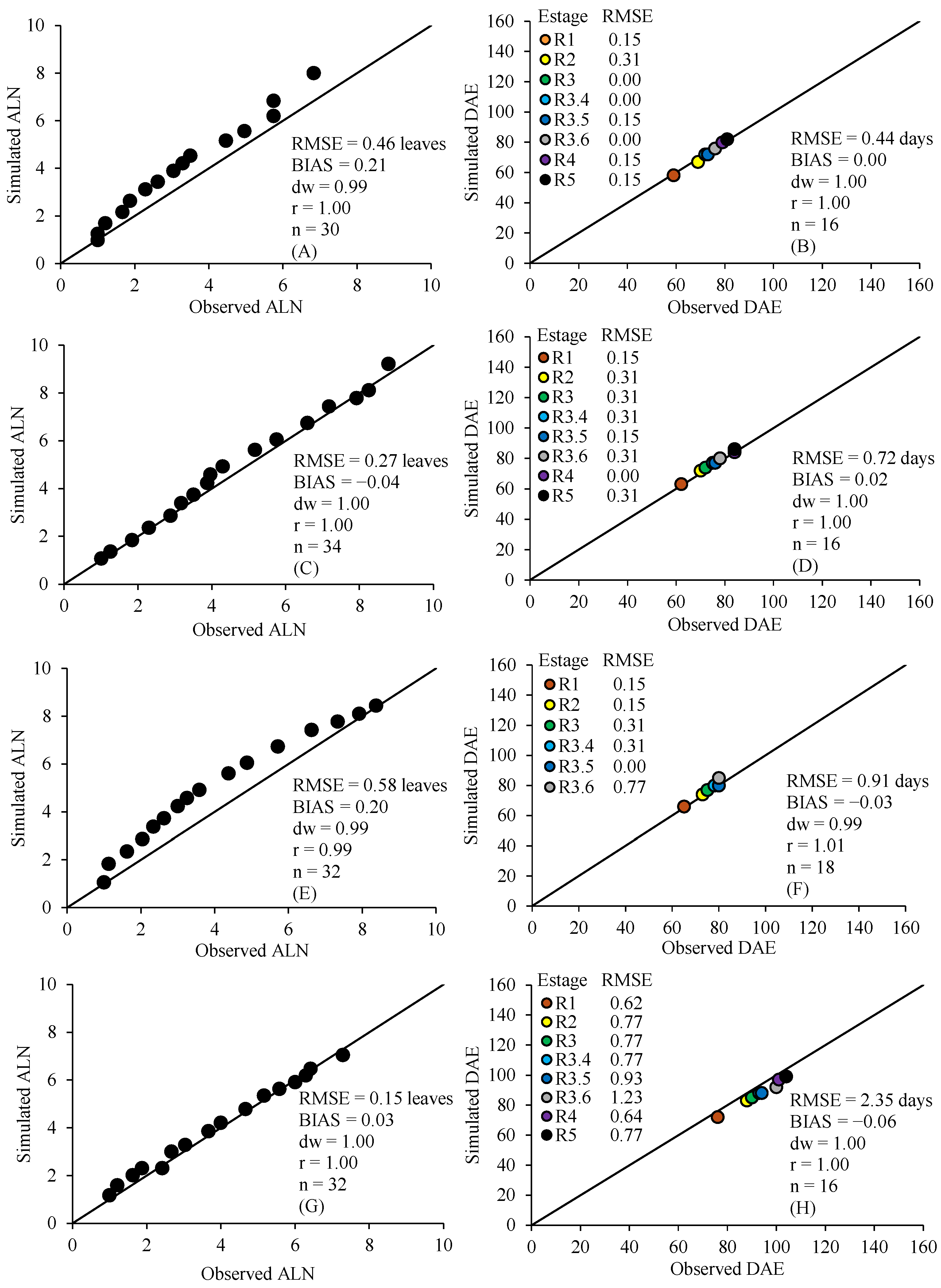
Figure A5.
Simulation from planting date (third season, Dourados/MS). Simulated versus observed accumulated leaf number (ALN) for the cultivars ‘Priscila’ (A), ‘Traderhorn’ (C), and ‘Red Beauty’ (E). Simulated versus observed days after planting (DAP) to reach phenological stages (R1.0 to R5) in the respective cultivars (B,D,F). The solid line represents the 1:1 ratio. The inset graphs represent the dispersion of residuals. RMSE = root mean square error; BIAS = bias index; dw = index of agreement; r = correlation coefficient; n = number of observations.
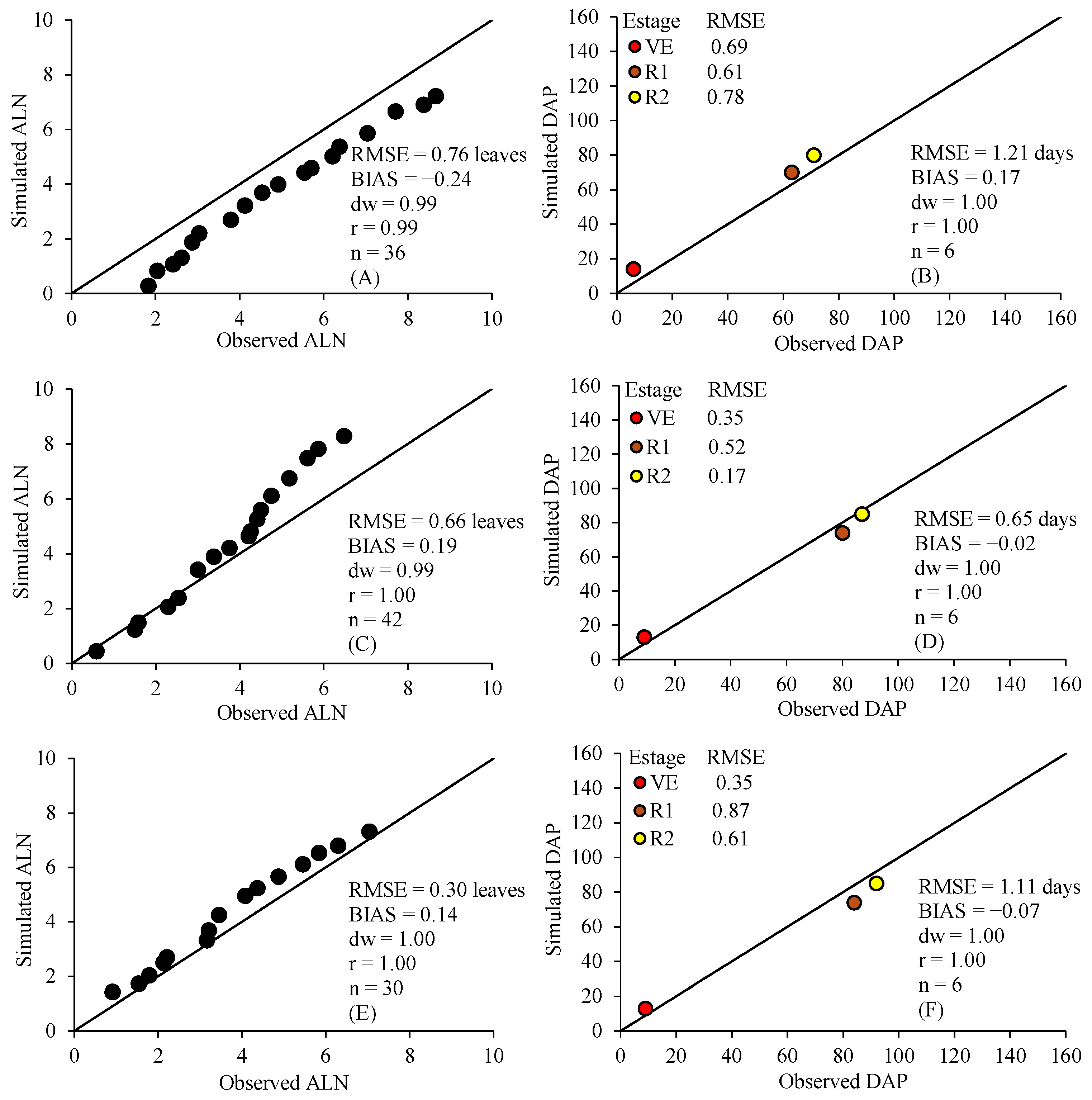
Figure A6.
Simulation from emergence date (third season, Dourados/MS). Simulated versus observed accumulated leaf number (ALN) for the cultivars ‘Priscila’ (A), ‘Traderhorn’ (C), and ‘Red Beauty’ (E). Simulated versus observed days after emergence (DAE) to reach phenological stages (R1.0 to R5) in the respective cultivars (B,D,F). The solid line represents the 1:1 ratio. The inset graphs represent the dispersion of residuals. RMSE = root mean square error; BIAS = bias index; dw = index of agreement; r = correlation coefficient; n = number of observations.
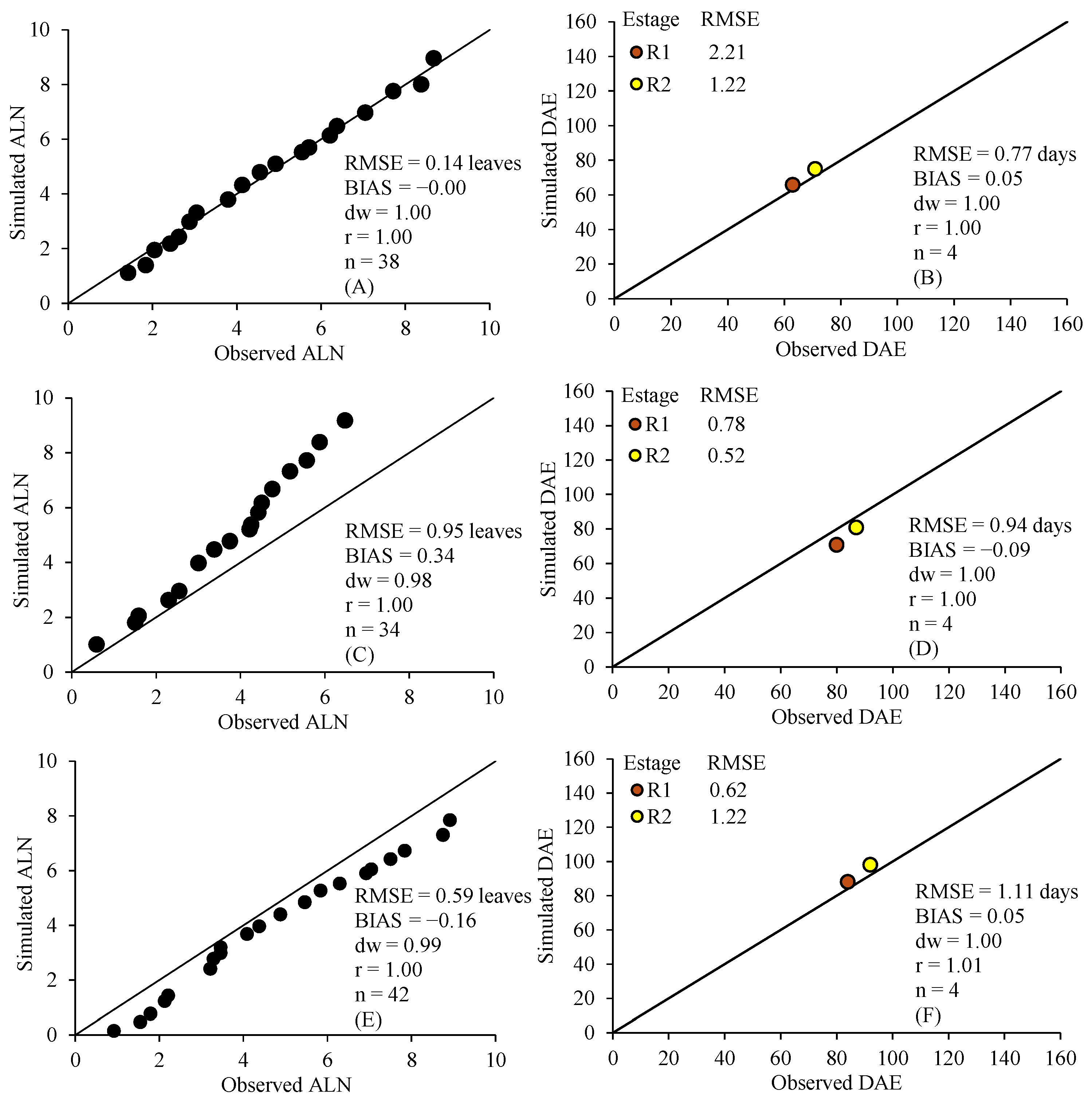
Figure A7.
Simulated versus observed developmental stages (DVS) as a function of days after planting (A) and days after emergence (B); and simulated versus observed vegetative stages (V) as a function of planting (C) and emergence (D) in Campo Grande/MS. Data for the cultivars ‘Jester’ (A,B) and ‘White Goddess’ (C,D). The solid line represents the 1:1 ratio.
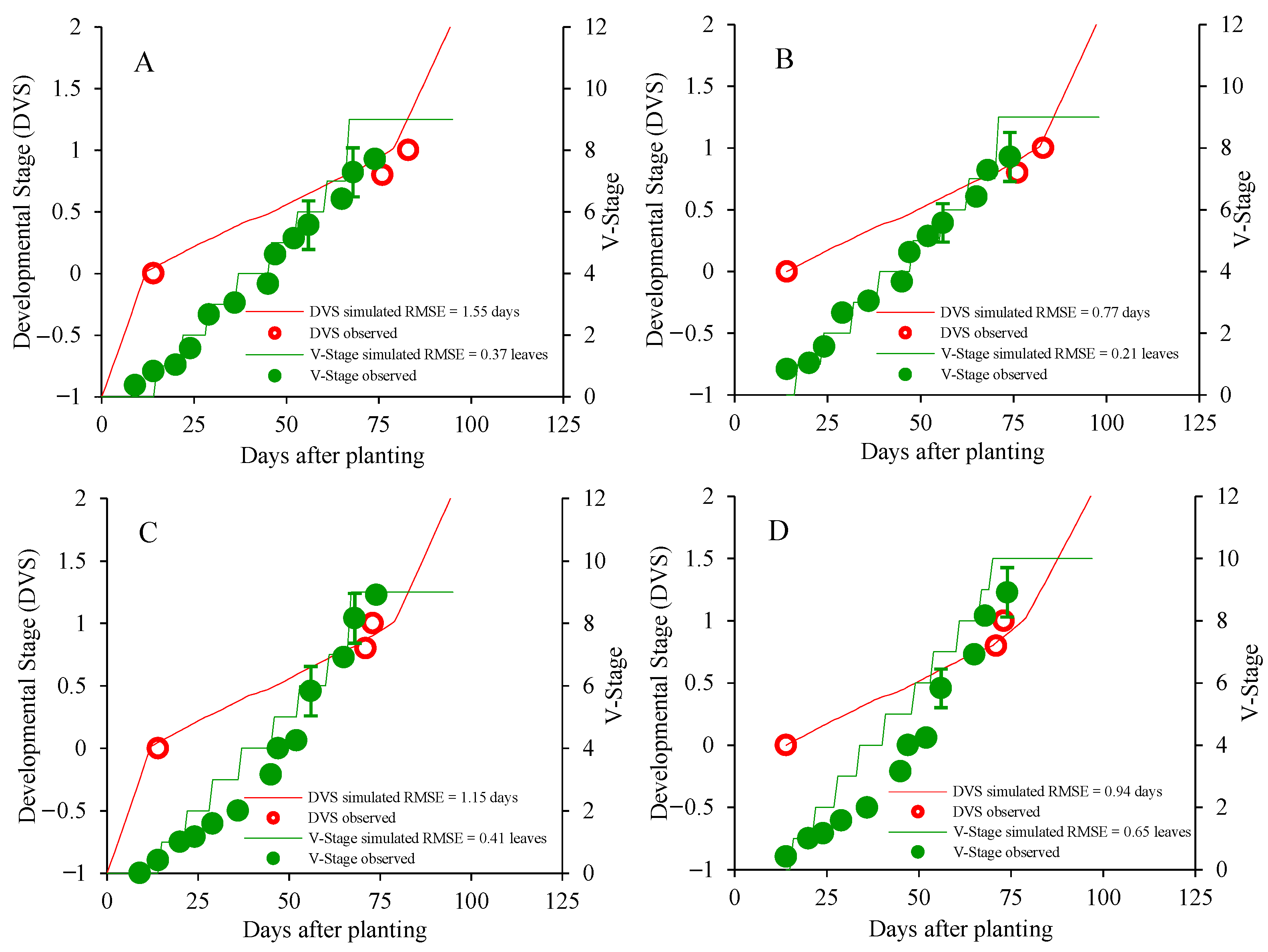
Figure A8.
Simulated versus observed developmental stages (DVS) as a function of days after planting (A) and days after emergence (B); and simulated versus observed vegetative stages (V) as a function of planting (C) and emergence (D) in Três Lagoas/MS. Data for the cultivars ‘Purple Flora’ (A,B) and ‘Jester’ (C,D). The solid line represents the 1:1 ratio.
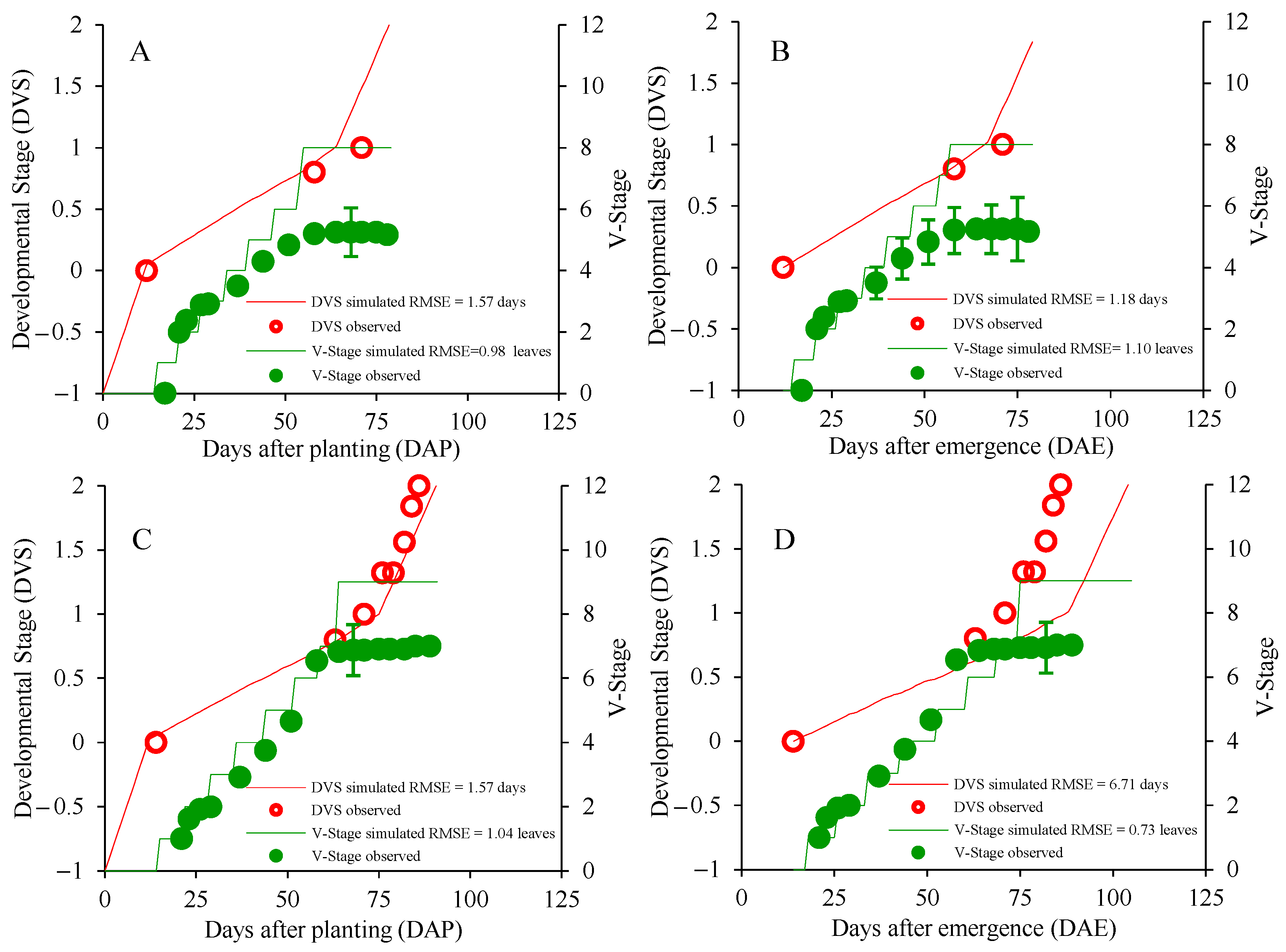
Figure A9.
Simulated versus observed developmental stages (DVS) as a function of days after planting (A) and days after emergence (B); and simulated versus observed vegetative stages (V) as a function of planting (C) and emergence (D) in Nova Andradina/MS. Data for the cultivars ‘Purple Flora’ (A,B) and ‘Peter Pears’ (C,D). The solid line represents the 1:1 ratio.
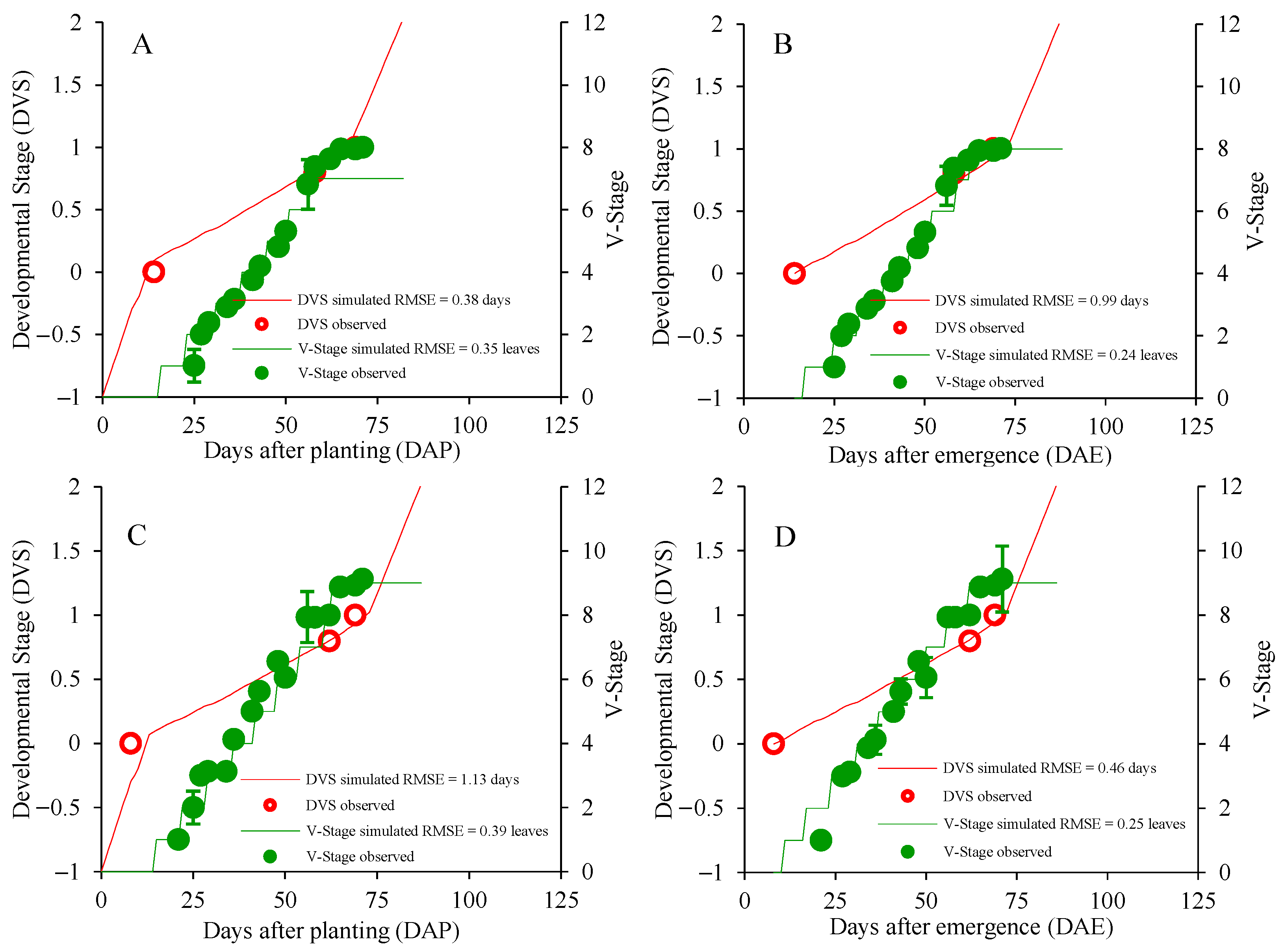
Figure A10.
Simulated versus observed developmental stages (DVS) as a function of days after planting (A) and days after emergence (B); and simulated versus observed vegetative stages (V) as a function of planting (C) and emergence (D) in Ponta Porã/MS. Data for the cultivars ‘Purple Flora’ (A,B) and ‘Peter Pears’ (C,D). The solid line represents the 1:1 ratio.
References
- Ikram, S.; Khalil, M.A.; Raza, M.Y. Climate resilient floriculture: Adapting cut flower and foliage production to a changing climate. In Climate Resilient Agriculture, 1st ed.; Ahmed, M., Ed.; Springer: Cham, Switzerland, 2025; Volume 2, pp. 353–373. [Google Scholar] [CrossRef] [Scilit]
- Bisbis, M.B.; Gruda, N.S.; Blanke, M.M. Securing Horticulture in a Changing Climate—A Mini Review. Horticulturae 2019, 5, 56. [Google Scholar] [CrossRef] [Scilit]
- Yeshiwas, Y.; Tadele, E.; Mohammed, A.; Hu, X. Impacts of climate change on horticultural systems with focus on socio-economic implications, production and postharvest challenges, and adaptive pathways. Discov. Environ. 2026, 4, 55. [Google Scholar] [CrossRef] [Scilit]
- Kadam, G.B.; Singh, K.P.; Singh, M.P. Effect of different temperature regimes on morphological and flowering characteristics in gladiolus (Gladiolus (Tourn) L.). Indian J. Plant Physiol. 2013, 18, 49–54. [Google Scholar] [CrossRef] [Scilit]
- Qayyum, M.M.; Hassan, I.; Khan, S.M.; Subhan, M.; Saleem, S.; Fiaz, S.; Alharbi, S.A.; Ansari, M.J. Analysis of dataset on reduction of high temperature stress by green net shade alleviate oxidative stress and augments the growth and vase life of gladiolus cut flower. Data Brief 2024, 54, 110378. [Google Scholar] [CrossRef] [Scilit]
- Uhlmann, L.O.; Streck, N.A.; Becker, C.C.; Schwab, N.T.; Benedetti, R.P.; Charão, A.S.; Ribeiro, B.S.M.R.; Silveira, W.B.; Backes, F.A.A.L.; Alberto, C.M.; et al. PhenoGlad: A model for simulating development in gladiolus. Eur. J. Agron. 2017, 82, 33–49. [Google Scholar] [CrossRef] [Scilit]
- Becker, D.; Paulus, D.; Bosco, L.C. Growth, development and quality of gladiolus ‘White Goddess’: Season, shade net, and mulching. Hortic. Bras. 2022, 40, 441–450. [Google Scholar] [CrossRef] [Scilit]
- Liu, W.; Bai, Y.; Du, T.; Li, M.; Yang, H.; Chen, S.; Lian, C.; Kang, S. Advances in regional-scale crop growth and associated process modeling. Sci. China Earth Sci. 2025, 68, 653–668. [Google Scholar] [CrossRef] [Scilit]
- Jones, J.W.; Antle, J.M.; Basso, B.; Boote, K.J.; Conant, R.T.; Foster, I.; Godfray, H.C.J.; Herrero, M.; Howitt, R.E.; Janssen, S.; et al. Brief history of agricultural systems modeling. Agric. Syst. 2017, 155, 240–254. [Google Scholar] [CrossRef] [Scilit]
- Tripathi, R.; Mohapatra, R.R.; Sahu, S.R.; Goud, B.R.; Debnath, M.; Jambhulkar, N.N. Crop modelling for impact assessment and identifying adaptation strategies under changing climate scenarios: A comprehensive review. Proc. Indian Natl. Sci. Acad. 2026, 1–19. [Google Scholar] [CrossRef] [Scilit]
- Wang, E.; Engel, T. Simulation of phenological development of wheat crops. Agric. Syst. 1998, 58, 1–24. [Google Scholar] [CrossRef] [Scilit]
- Streck, N.A.; Weiss, A.; Xue, Q.; Baenziger, P.S. Improving predictions of developmental stages in winter wheat: A modified Wang and Engel model. Agric. For. Meteorol. 2003, 115, 139–150. [Google Scholar] [CrossRef] [Scilit]
- Bonatto, M.I.; Bosco, L.C.; Pandolfo, C.; Stanck, L.T.; Souza, A.G.; Rossato, O.B.; Streck, N.A. PhenoGlad model and the zoning of gladiolus planting dates in the state of Santa Catarina, Brazil. Agrometeoros 2023, 31, e027299. [Google Scholar] [CrossRef] [Scilit]
- Becker, D.; Paulus, D.; Bosco, L.C.; Hojo, E.T.D.; Sato, A.J.; Yamamoto, L.Y.; Ritter, G.; Nava, G.A. Validation of the PhenoGlad model and determination of planting dates of gladiolus for the state of Paraná. Semin. Cienc. Agrar. 2023, 44, 39–60. [Google Scholar] [CrossRef] [Scilit]
- Jhanji, S.; Kaur, R. Evaluation of PhenoGlad model on phenological development of gladiolus varieties under subtropical conditions of Punjab. J. Agrometeorol. 2022, 24, 411–414. [Google Scholar] [CrossRef] [Scilit]
- Nascimento, Y.Y.G.D.; Pereira, V.S.; Xavier, T.L.S.; Figueredo, H.F.; Lima, L.G.; Souza, R.R.; Uhlmann, L.O.; Beckmann-Cavalcante, M.Z. Gladiolus harvest simulation using the PhenoGlad model for different marketing periods. Rev. Caatinga 2024, 37, e12446. [Google Scholar] [CrossRef] [Scilit]
- Hofmann, G.S.; Silva, R.C.; Weber, E.J.; Barbosa, A.A.; Oliveira, L.F.B.; Alves, R.J.V.; Hasenack, H.; Aquino, F.E.; Cardoso, M.F. Changes in atmospheric circulation and evapotranspiration are reducing rainfall in the Brazilian Cerrado. Sci. Rep. 2023, 13, 11236. [Google Scholar] [CrossRef] [Scilit] [PubMed]
- de Oliveira Aparecido, L.E.; Lorençone, P.A.; Lorençone, J.A.; Meneses, K.C.M.; Moraes, J.R.S.C. Climate changes and their influences in water balance of Pantanal biome. Theor. Appl. Climatol. 2021, 143, 659–674. [Google Scholar] [CrossRef] [Scilit]
- Souza, A.; Abreu, M.C.; Oliveira-Júnior, J.F.d.; Aristone, F.; Fernandes, W.A.; Aviv-Sharon, E.; Graf, R. Climate Regionalization in Mato Grosso do Sul: A Combination of Hierarchical and Non-hierarchical Clustering Analyses Based on Precipitation and Temperature. Braz. Arch. Biol. Technol. 2022, 65, e22210331. [Google Scholar] [CrossRef] [Scilit]
- de Oliveira Aparecido, L.E.; da Silva Cabral de Moraes, J.R.; de Meneses, K.C.; Torsoni, G.B.; Lima, R.F.; Costa, C.T.S. Köppen-Geiger and Camargo climate classifications for the Midwest of Brasil. Theor. Appl. Climatol. 2020, 142, 1133–1145. [Google Scholar] [CrossRef] [Scilit]
- Schwab, N.T.; Streck, N.A.; Becker, C.C.; Langner, J.A. A phenological scale for the development of gladiolus. Ann. Appl. Biol. 2015, 166, 496–507. [Google Scholar] [CrossRef] [Scilit]
- Janssen, P.H.M.; Heuberger, P.S.C. Calibration of process-oriented models. Ecol. Model. 1995, 83, 55–66. [Google Scholar] [CrossRef] [Scilit]
- Leite, H.G.; Andrade, V.C.L. Um método para condução de inventários florestais sem o uso de equações volumétricas. Rev. Arvore 2002, 26, 321–328. [Google Scholar] [CrossRef] [Scilit]
- Willmott, C.J. On the validation of models. Phys. Geogr. 1981, 2, 184–194. [Google Scholar] [CrossRef] [Scilit]
- Javaid, A.; Pandey, R.K.; Shah, A.H.; Bakshi, P.; Nazki, I.T.; Kaushal, N.; Chand, G.; Dogra, S.; Kumar, R.; Singh, A.K.; et al. Response of Gladiolus grandiflorus varieties to planting date: Effects on growth, flowering, and vase life. BMC Plant Biol. 2025, 25, 481. [Google Scholar] [CrossRef] [Scilit] [PubMed]
- Singh, S.; Sehrawat, S.K.; Sharma, S. Effect of Planting Time and Growing Conditions on Sprouting and Growth of Gladiolus Cv. American Beauty. Int. J. Curr. Microbiol. Appl. Sci. 2019, 8, 656–662. [Google Scholar] [CrossRef] [Scilit]
- Marfoua, M.; Buisson, E.; Bissati-Bouafia, S.; Eddoud, A.; Benchettouh, A. Improving seed germination of native species for camel rangeland restoration: Effects of cold stratification and temperature. Bot. Lett. 2023, 170, 303–317. [Google Scholar] [CrossRef] [Scilit]
- Sajjad, Y.; Jaskani, M.J.; Mehmood, A.; Qasim, M.; Akhtar, G. Alleviation of gladiolus corm dormancy through application of 6-benzylaminopurine and gibberellic acid. Pak. J. Bot. 2020, 52, 831–838. [Google Scholar] [CrossRef] [Scilit]
- Li, J.; Seng, S.; Li, D.; Zhang, F.; Liu, Y.; Yao, T.; Liang, J.; Yi, M.; Wu, J. Antagonism between abscisic acid and gibberellin regulates starch synthesis and corm development in gladiolus. Hortic. Res. 2021, 8, 155. [Google Scholar] [CrossRef] [Scilit]
- Liang, J.H.; Li, J.R.; Liu, C.; Pan, W.Q.; Wu, W.J.; Shi, W.J.; Wang, L.J.; Yi, M.F.; Wu, J. GhbZIP30-GhCCCH17 module accelerates corm dormancy release by reducing endogenous ABA under cold storage in gladiolus. Plant Cell Environ. 2023, 46, 2078–2096. [Google Scholar] [CrossRef] [Scilit]
- Blanchard, M.G.; Runkle, E.S.; Fisher, P.S. Modeling plant morphology and development of petunia in response to temperature and photosynthetic daily light integral. Sci. Hortic. 2011, 129, 313–320. [Google Scholar] [CrossRef] [Scilit]
- Paiva, P.D.O.; Almeida, E.F.A. Produção de Flores de Corte, 1st ed.; UFLA: Lavras, Brazil, 2012; 678p. [Google Scholar]
- Grossiord, C.; Buckley, T.N.; Cernusak, L.A.; Novick, K.A.; Poulter, B.; Siegwolf, R.T.W.; Sperry, J.S.; McDowell, N.G. Plant responses to rising vapor pressure deficit. New Phytol. 2020, 226, 1550–1566. [Google Scholar] [CrossRef] [Scilit]
- López, J.; Way, D.A.; Sadok, W. Systemic effects of rising atmospheric vapor pressure deficit on plant physiology and productivity. Glob. Change Biol. 2021, 27, 1704–1720. [Google Scholar] [CrossRef] [Scilit]
- Dong, X.; Li, B.-L.; Yan, Z.; Guan, L.; Huang, S.; Li, S.; Qi, Z.; Tang, L.; Tian, H.; Fu, Z.; et al. Impacts of High Temperature, Relative Air Humidity, and Vapor Pressure Deficit on Seed Set of Contrasting Maize Genotypes during Flowering. J. Integr. Agric. 2023, 23, 2955–2969. [Google Scholar] [CrossRef] [Scilit]
- Santos, J.J.S.; Pêgo, R.G.; Couto, B.R.M.; Bueno, M.M.; Carvalho, D.F. Evaluation of water requirement, commercial quality, and yield response factor of gladiolus produced with automated irrigation in different growing periods. Cienc. Agrotec. 2020, 44, e017220. [Google Scholar] [CrossRef] [Scilit]
- Mazzini-Guedes, R.B.; Guedes Filho, O.; Bonfim-Silva, E.M.; Couto, J.C.C.; Pereira, M.T.J.; Silva, T.J.A. Management of corm size and soil water content for gladiolus flower production. Ornam. Hortic. 2017, 23, 152–159. [Google Scholar] [CrossRef] [Scilit]
- Porto, R.d.A.; Koetz, M.; Bonfim-Silva, E.M.; Polizel, A.C.; Silva, T.J.A. Effects of water replacement levels and nitrogen fertilization on growth and production of gladiolus in a greenhouse. Agric. Water Manag. 2014, 131, 50–56. [Google Scholar] [CrossRef] [Scilit]
- Rizwan, M.; Akhtar, G.; Shehzad, M.A.; Aloufi, S.; Alghanem, S.M.S.; Zulfiqar, F. Chitosan induces water deficit stress tolerance in gladiolus. Plant Biosyst. 2025, 159, 1552–1568. [Google Scholar] [CrossRef] [Scilit]
- Shillo, R.; Halevy, A.H. The effect of various environmental factors on flowering of gladiolus. III. Temperature and moisture. Sci. Hortic. 1976, 4, 147–155. [Google Scholar] [CrossRef] [Scilit]

Disclaimer/Publisher’s Note: The statements, opinions and data contained in all publications are solely those of the individual author(s) and contributor(s) and not of MDPI and/or the editor(s). MDPI and/or the editor(s) disclaim responsibility for any injury to people or property resulting from any ideas, methods, instructions or products referred to in the content. |
© 2026 by the authors. Licensee MDPI, Basel, Switzerland. This article is an open access article distributed under the terms and conditions of the Creative Commons Attribution (CC BY) license.