A Machine Learning Framework for Crop Productivity Classification and Risk Assessment

Abstract

Knowing in advance which fields are likely to yield poorly has obvious value for farm management, insurance, and logistics, yet reliable field-scale productivity classification and risk assessment from satellite data remain open problems. We present a machine learning framework for crop productivity classification and pre-harvest yield risk assessment for corn, soybean, and wheat in western Paraná, Brazil, integrating a harmonized Landsat/Sentinel-2 time-series with gridded climate variables and phenological features. The framework evaluates four algorithms on two tasks: three-class productivity classification (Low, Medium, High) and binary risk assessment (Low vs. Not Low), where a field flagged as Low is treated as at risk of poor yield before harvest. Early in the analysis, a single temporal feature, harvest_day_of_year, was found to account for 47–64% of model importance and to produce near-identical results across all five initially tested algorithms, a sign of near-deterministic separation rather than a genuine predictive signal. We excluded this feature and reported results on the remaining pre-harvest predictors only. For the binary risk assessment task, three algorithms achieved 84.5% accuracy for wheat and 74.9% for soybean using only pre-harvest features. For corn, ablation revealed that vegetation features contain genuine discriminative signal previously obscured: three algorithms now exceed the dummy baseline, versus only one before ablation. The wheat binary risk model shows strong application potential for early warning of yield risk; corn requires additional data, most likely more growing seasons covering a wider range of climate conditions, before it can be used reliably.

1. Introduction

A farmer who knows three weeks before harvest that one field is headed for a poor yield can redirect inputs, adjust storage plans, or file an insurance claim with supporting evidence. Performing this at a scale, across hundreds of fields and multiple crops, is not feasible by visual inspection alone. Satellite-based classification offers a scalable alternative, but the agronomic literature is inconsistent on how well it actually works in practice.

Corn (Zea mays), soybean (Glycine max), and wheat (Triticum aestivum) are the three main crops in western Paraná and are collectively central to Brazilian agribusiness. A key practical advantage of satellite-based classification is that the entire prediction pipeline can operate without any field visits: all inputs (HLS surface reflectance and NASA POWER climate data) are freely available through public archives and APIs, meaning risk assessments can, in principle, be generated for any field with a known location and harvest calendar. Benos et al. [1] identify yield prediction as one of the most critical and most difficult sub-tasks in agricultural machine learning (ML), requiring models to integrate environmental, phenological, and management signals simultaneously. Most published work addresses this with a single sensor and a single algorithm, making it hard to know whether the reported accuracy reflects the model or the quality of the underlying features.

Two specific gaps motivated this work. First, most studies use one satellite mission, which creates temporal gaps when cloud cover is high. The Harmonized Landsat and Sentinel-2 (HLS) dataset [2] combines both missions into a single surface reflectance product, substantially increasing the number of cloud-free observations per growing season. Second, snapshot spectral indices are known to be less informative than features that summarize the full crop cycle [3,4], yet few field-scale classification studies have systematically evaluated both.

NDVI [5] is the most widely used crop vigor proxy, contrasting near-infrared reflectance from healthy tissue against red-band chlorophyll absorption. Ensemble methods, particularly Random Forest and Gradient Boosting, have consistently outperformed single classifiers on agronomic data [1]. Random Forest reduces variance by averaging de-correlated trees; Gradient Boosting reduces bias by fitting residuals sequentially, which tends to help when the signal is concentrated in hard-to-classify examples.

Recent advances in sequence modeling have opened a complementary path. Long Short-Term Memory networks [6] and temporal Convolutional Networks [7] applied directly to satellite time-series have achieved strong results in crop type mapping and yield regression, without requiring the manual feature engineering that scalar-summary approaches depend on. Data-fusion architectures combining optical imagery with radar or climate streams have further improved robustness under cloudy conditions [8]. These sequence-based methods represent the logical next step beyond the framework presented here; the present study establishes a rigorously validated scalar-feature baseline against which such models should be compared.

We pursued four objectives: (1) building a reproducible HLS-plus-climate pipeline; (2) engineering temporal and phenological features from the full crop cycle; (3) comparing four classifiers on the same feature set for both three-class productivity classification and binary low-productivity risk assessment; and (4) running an ablation study to confirm that the predictive signal used for risk detection comes from genuine agronomic features rather than from proxies for harvest timing.

In this study, low productivity is operationally defined as yield falling below the lowest tercile of the training distribution for each crop. A field classified as Low is treated as at risk of poor yield before harvest; classification is the mechanism through which risk assessment is performed. We acknowledge that this threshold has no direct agronomic interpretation, such as a break-even yield; anchoring it to external economic benchmarks is a recommended extension. On the data side, HLS substantially increases cloud-free observation frequency compared with either sensor alone, but the harmonization process introduces an occasional processing lag and may leave residual inter-sensor differences that could affect near-real-time applications.

The primary contribution of this study is the ablation methodology itself: the identification, diagnosis, and removal of harvest_day_of_year as a near-deterministic leakage feature, and the demonstration that the remaining pre-harvest feature set produces a genuinely discriminative signal for wheat and soy low-productivity risk detection. This approach provides a transferable template for detecting and correcting dominant-feature artifacts in agricultural classification pipelines.

2. Materials and Methods

2.1. Study Area

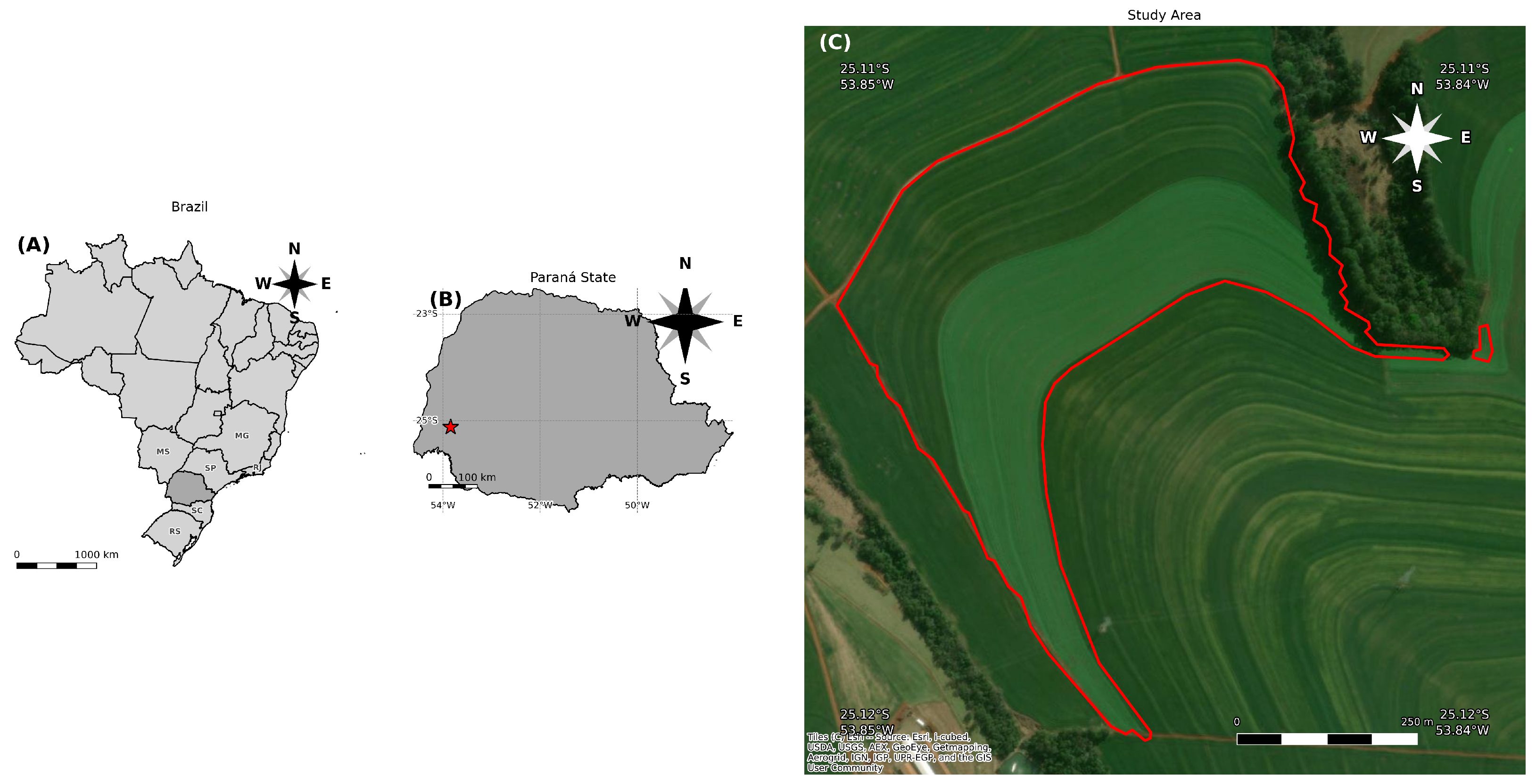
The study area covers agricultural fields in western Paraná state, Brazil (Figure 1). The sampled area spans a bounding box of approximately 916 m (N–S) × 708 m (E–W) (≈64.9 ha).

Ground-truth productivity data (t/ha) were collected from combine harvester yield monitors and aggregated to 2560 unique 10 × 10 m grid cells, covering a total sampled area of approximately 25.6 ha (approximately 39% of the bounding box). The remaining area within the bounding box corresponds to roads, field borders, and areas not covered by the yield monitor during the harvest seasons included in this study.

Each grid cell contains between 1 and 24 yield monitor points (mean: 7.5; median: 7), which were averaged to obtain the cell-level productivity value used as the model target.

Data were available for the following crop-season combinations: corn in five seasons (2013 S1, 2016 S2, 2023 S1, 2025 S2, 2026 S1; 13,905 observations); the 2026 S1 corn season (typically harvested February–March in western Paraná) was complete prior to manuscript submission; soy in five seasons (2014 S1, 2015 S1, 2016 S1, 2017 S1, 2025 S1; 12,258 observations); and wheat in two seasons only (2013 S2, 2014 S2; 3672 observations). The non-contiguous multi-year range was intentional: including both drought years and favorable seasons gives the models exposure to climatic variability and reduce the risk of learning season-specific patterns. However, the wheat dataset covers only two growing seasons, which limits the generalizability of the wheat models and should be considered when interpreting those results.

An important spatial consideration is that the 75/25 train-test split was performed at the grid-cell level. Individual field polygon boundaries are not stored in the final modeling dataset, so field counts and field-level size statistics cannot be reported directly.

Because the 2560 grid cells are spatially contiguous (with a maximum nearest-neighbor distance of 9.86 m between adjacent cells), meaning cells that are physically close to each other can appear in both training and test sets. No spatial blocking or field-level splitting was applied.

This spatial autocorrelation may cause accuracy estimates to be slightly optimistic relative to what would be achieved when predicting on spatially independent locations. A spatial block split [9] would provide a more conservative performance estimate and is recommended for future work. The current results should therefore be interpreted as an upper bound on performance within the same study area.

2.2. Data Processing and Feature Engineering Workflow

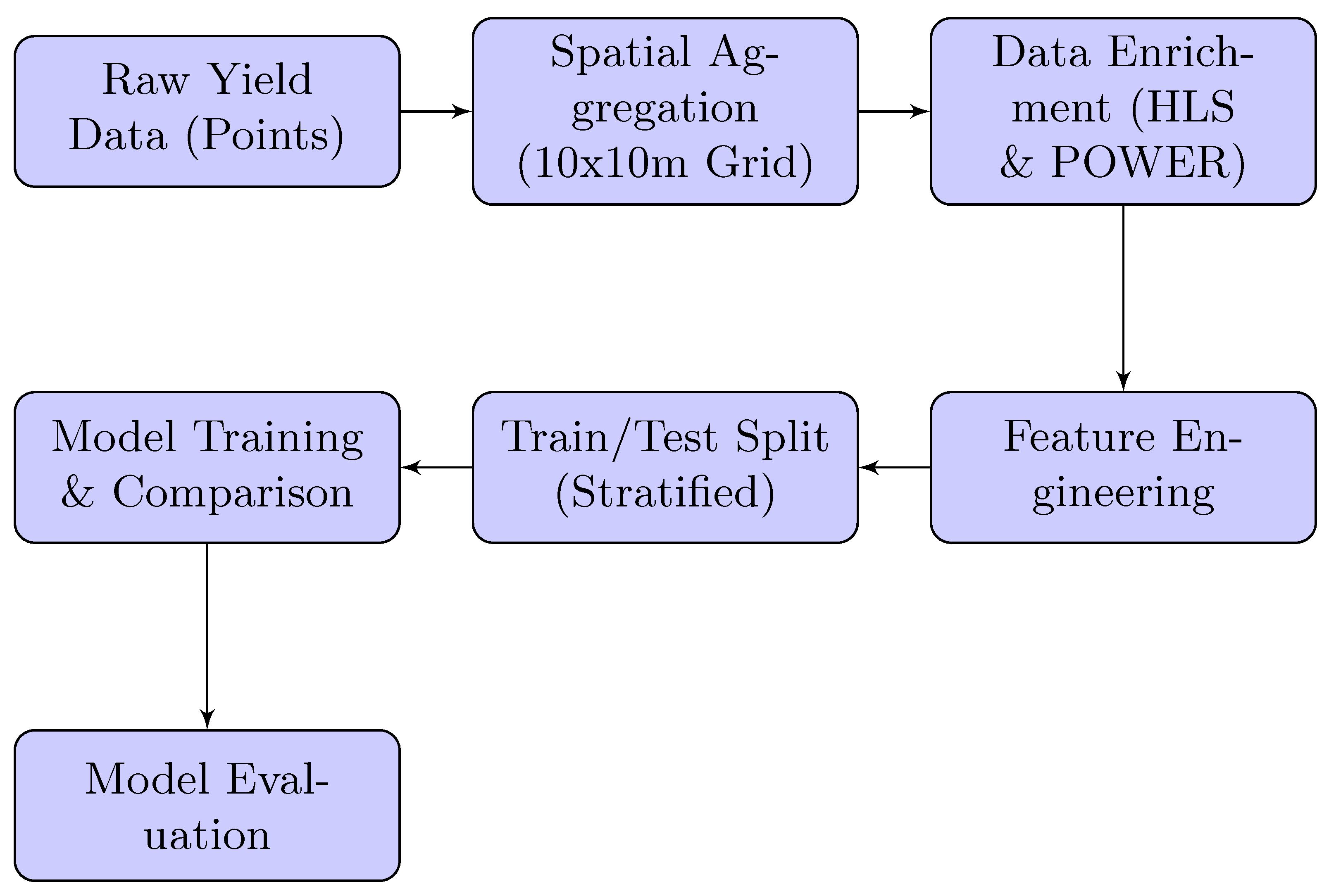
Figure 2 summarizes the full pipeline.

2.2.1. Spatial Aggregation and Cleaning

Raw yield monitor points were filtered with a per-crop, per-year interquartile range (IQR) criterion to remove harvester operation artifacts (stops, speed changes). Filtering per-crop and per-year rather than globally ensures that genuine inter-annual yield differences are not treated as outliers. The cleaned points were then aggregated to a 10 × 10 m grid by taking the mean productivity per cell, matching the native Sentinel-2 resolution.

2.2.2. Data Enrichment from External Sources

Satellite reflectance came from HLS v2.0 [2], which harmonizes Sentinel-2 MultiSpectral Instrument (MSI) and Landsat-8 Operational Land Imager (OLI) observations by correcting for Bidirectional Reflectance Distribution Function (BRDF) effects. Clouds and cloud shadows were masked using the Fmask-based Quality Assessment (QA) band provided with each HLS granule, which flags pixels as clear, water, cloud shadow, adjacent cloud, cloud, or cirrus; only pixels with the clear flag were retained. As an additional quality filter, observations with NDVI $\ge 0.99$ were also flagged as cloud-affected and excluded, since physically unrealistic saturation values indicate residual contamination not captured by Fmask.

The resulting clear-sky observations are irregularly spaced in time because cloud events remove some acquisition dates entirely. To reconstruct a continuous daily vegetation index series, we applied a Whittaker smoother with a regularization parameter $\lambda =100$, which has been shown to perform well for dense agricultural time-series without introducing the end-of-series distortion associated with moving-average or polynomial filters [10]. The smoothing fully resolved all cloud-induced gaps: zero missing values remain in the NDVI and EVI features of the final dataset. From the smoothed daily series, we derived NDVI and EVI (Enhanced Vegetation Index). Daily climate variables (precipitation, temperature, solar radiation, vapor pressure deficit) were obtained from NASA POWER [11].

2.3. Feature Description

Table 1. Remote sensing and aggregated climate features.

Feature Name	Description	Details and Units
Remote Sensing Features (Vegetation)
peak_ndvi_to_date	Maximum NDVI until the forecast cutoff.	Peak plant vigor. Range: $-1$ to 1.
ndvi_at_cutoff	NDVI on the last available day.	Vigor at prediction time.
evi_at_cutoff	EVI on the cutoff date.	Less prone to canopy saturation than NDVI.
ndvi_auc_to_date	Area under the NDVI curve.	Cumulative photosynthetic activity over the cycle.
ndvi_std_to_date	Standard deviation of NDVI.	Elevated values suggest stress episodes or uneven development.
green_up_slope_to_date	Slope of NDVI during green-up.	Higher values indicate faster early-season development.
senescence_slope	Rate of NDVI decline after peak.	Slow decline may indicate stress; fast decline, early maturity.
days_since_peak_at_cutoff	Days elapsed since peak NDVI.	How far the crop has progressed into senescence.
Accumulated and Aggregated Climate Features
cum_gdd_base_10_to_date	Growing Degree Days (GDD) accumulated above 10 °C.	Thermal units for corn and soy. Unit: °C-day.
cum_gdd_base_0_to_date	GDD accumulated above 0 °C.	Thermal units for wheat. Unit: °C-day.
cum_srad_to_date	Accumulated solar radiation.	Total photosynthetically available energy. Unit: MJ/m2.
mean_vpd_to_date	Mean Vapor Pressure Deficit.	Atmospheric dryness stress. Unit: kPa.
useful_srad_vs_vpd	Radiation discounted for Mean Vapor Pressure Deficit (VPD) stress.	Net energy available under dry-air conditions.

and 

Table 2. Growth-stage and rolling-window climate features.

Feature Name	Description	Details and Units
Rolling Window Climate Features
precip_7d	Precipitation in the 7 days before cutoff.	Unit: mm.
precip_30d	Precipitation in the 30 days before cutoff.	Unit: mm.
t2m_mean_30d	Mean temperature in the 30 days before cutoff.	Unit: °C.
Climate Features by Growth Stage
mean_t2m_[stage]	Mean air temperature during the stage.	Unit: °C.
total_precip_[stage]	Total precipitation during the stage.	Unit: mm.
dry_days_[stage]	Days with precipitation < 1 mm.	Unit: days.
inter_heat_dry_[stage]	Heat × dry-day interaction.	Combined heat–drought stress index.

list the full feature set. All features are computed from observations available up to a fixed prediction cutoff set at 30 days before the expected harvest date for each crop-season combination (prediction_lag_days = 30), following the agronomic calendars cited below. This 30-day horizon ensures that the model receives only information observable before harvest while still capturing late-season climate and spectral signals that are predictive of final yield.

Climate variables were aggregated over phenological windows defined by fixed day-counts before harvest, following established agronomic calendars for the region [12,13]. Fixed calendar-day windows are a deliberate simplification: crop development is strongly influenced by inter-annual temperature variability, and a window defined as “days 40–70 before harvest” will not always correspond to the same physiological stage in a cool versus a warm year. Dynamic alternatives, such as NDVI-based phenology detection (deriving stage boundaries from green-up or senescence inflection points in the smoothed NDVI curve) or Growing Degree Day (GDD) thresholds, would more accurately track actual development. We chose fixed windows because they require no additional assumption about phenological models and are directly reproducible from the public agronomic calendars cited; future work should assess whether dynamic stage boundaries improve predictive performance. Features tied to growth stages that do not exist for a given crop (e.g., total_precip_PodFormation for corn) received MI scores of zero and were excluded automatically.

Two vegetation indices were derived from the smoothed HLS time-series: NDVI and EVI. NDVI was selected as the primary canopy greenness proxy owing to its near-universal adoption in crop monitoring and interpretability. EVI was included because it is less susceptible to canopy saturation at high biomass densities (a known limitation of NDVI for dense corn and soy canopies) and incorporates a soil-adjustment term that reduces background reflectance contamination early in the season [10]. Red-edge indices (e.g., NDRE) were considered but not included because consistent red-edge bands are available from Sentinel-2 MSI only and not from Landsat-8 OLI, which would have introduced a systematic difference in index availability depending on the satellite overflight contributing to a given observation. Incorporating red-edge information from Sentinel-2-only composites is a recommended extension.

A key limitation that affects all three crops, and corn in particular, is the relatively small number of growing seasons available. Since the framework is designed to operate exclusively from remote sensing and climate data—requiring no field visits or external ground records—it relies on the spectral and climate signal to capture all relevant yield drivers. Corn covers five seasons spanning 2013–2026, but with non-contiguous years and contrasting planting windows (S1 and S2), the inter-seasonal variability captured may not be sufficient to fully separate productivity classes. The corn results (Section 3.5) demonstrate that identical NDVI profiles can correspond to substantially different yield outcomes across years, which is the pattern expected when yield variation is driven by factors that change between seasons, but are not fully resolved by the available remote sensing and climate features in those years. Expanding the number of seasons is the highest-priority extension for corn and soybean within this remote-sensing-only framework.

2.4. Machine Learning Modeling and Evaluation

Productivity was classified into three tiers (Low, Medium, High) using tercile splits of the training yield distribution. The tercile approach was chosen primarily for methodological simplicity and reproducibility, as it produces balanced classes without assumptions about the shape of the yield distribution. We acknowledge that the resulting class boundaries, particularly the narrow 0.64 t/ha soy Medium range, are not anchored to agronomic thresholds such as break-even yields or historical regional averages. Future work should consider clustering-based methods (e.g., K-Means or Gaussian Mixture Models) or economically motivated boundaries that would give the tiers clearer operational meaning. Applying training-set boundaries to the test set, rather than recomputing them, is critical: recomputing would allow information about the test distribution to influence the class definitions.

We compared four classifiers: Random Forest (RF), Gradient Boosting (GB), Logistic Regression (LR, as a linear baseline), and K-Nearest Neighbors (KNN). LR and KNN are scale-sensitive and were wrapped in a StandardScaler pipeline; RF and GB were applied to raw values.

2.4.1. Class Imbalance Handling

The binary task introduces a 2:1 class imbalance (Not Low, approximately twice as frequent as Low across all three crops). Class imbalance was addressed differently across algorithms. For RF, the class_weight = ‘balanced’ parameter was used, which re-weights each tree’s split criterion by the inverse class frequency. For LR, the same class_weight = ‘balanced’ option was applied to the loss function. GB and KNN do not expose a direct class-weight parameter in scikit-learn. For GB, no explicit class-weighting mechanism was applied; GB’s sequential boosting naturally assigns higher weight to misclassified examples in subsequent iterations, which tends to give some implicit attention to minority-class errors, but this is not equivalent to explicit class reweighting. The subsample parameter included in the search grid (0.7, 0.85, 1.0) serves as a stochastic regularizer, not as a class-balancing strategy. We acknowledge this as a limitation: GB in this study was not explicitly balanced, and future work should apply SMOTE or sample weights uniformly before all classifiers to make the comparison more controlled. For KNN, the weights = ‘distance’ option was used, which down-weights the influence of the more numerous Not-Low neighbors relative to nearby Low neighbors. We acknowledge that these strategies are not equivalent in strength, and future work should explicitly compare re-sampling techniques (e.g., SMOTE) applied uniformly before all classifiers.

A preliminary run with all five algorithms, including the Support Vector Machine (SVM), revealed something unexpected: harvest_day_of_year alone accounted for 47–64% of Gini importance across all models, and the binary wheat task reached 98.7% accuracy identically across all five algorithm families. When a Logistic Regression and a tuned Gradient Boosting produce the same result to the decimal point, the classification is not being driven by the model; it is being driven by one feature. We removed harvest_day_of_year from the feature set and report all results below on the remaining predictors. SVM was also dropped from the final comparison due to its substantially longer training time without offering additional interpretability or feature importance information. In the unablated configuration, SVM achieved three-class accuracies of 52.2% (corn), 53.9% (soy), and 68.9% (wheat), and binary accuracies of 62.3% (corn), 72.6% (soy), and 98.7% (wheat)—results consistent with the other four algorithms and with the conclusion that algorithm choice is secondary to feature quality.

Feature selection used Mutual Information (MI), computed once on the full training set (not within each CV fold), retaining the top 10 features from approximately 57–64 candidates. Computing MI outside the CV loop is a known potential source of optimistic bias, as the selector has access to the entire training distribution when ranking features; this limitation is acknowledged and should be corrected in future work by nesting MI selection inside each CV fold. The threshold of 10 features was set as a fixed configuration parameter; future work should assess whether a performance-curve analysis would identify a different optimal value for each crop.

Hyperparameters were tuned by randomized search with 30 iterations, 5-fold stratified Cross-Validation (CV), and macro-F1 scoring. This iteration count was a computational constraint; globally optimal hyperparameters may not have been found, particularly for RF and GB given the size of their search spaces. For RF: n_estimators 100–500, max_depth {5, 10, 15, 20, None}, min_samples_split {2, 5, 10}, min_samples_leaf {1, 2, 4}, max_features {‘sqrt’, ‘log2’, 0.5}. For GB: n_estimators 100–300, learning_rate {0.05, 0.1, 0.2}, max_depth {3, 5, 7}, subsample {0.7, 0.85, 1.0}, max_features {‘sqrt’, ‘log2’}. For LR: C {0.01–100}, penalty {L1, L2}, solver. For KNN: k {5, 11, 21, 31, 51}, weighting {uniform, distance}, metric {Euclidean, Manhattan}. Class weights were set to ‘balanced’ for RF and LR.

Data were split 75/25 with stratification. A majority-class dummy classifier provided baselines of 33.3% (three-class) and 66.7% (binary). Performance was assessed by overall accuracy, macro-averaged F1, and per-class precision, recall, and F1.

All analyses were performed using Python 3.12 with scikit-learn 1.6.1, shap 0.51.0, pandas 2.2.2, numpy 2.0.2, matplotlib 3.10.0, and seaborn 0.13.2. Earth Engine data access used the earthengine-api 1.7.22 client library. NASA POWER data were retrieved via the POWER Data Access Viewer REST API.

2.4.2. Binary Classification for Risk Assessment

As a secondary analysis, Medium and High productivity classes were merged into a single Not Low class, framing the problem as binary low-productivity risk detection. A grid cell is considered at risk when the model predicts Low productivity, where Low is defined as yield below the training-set first tercile (the same threshold used for the three-class task). This operational definition means the risk indicator is directly linked to the yield distribution observed in the training data: a field flagged as at risk has a predicted productivity in the lowest third of the historical range for that crop.

The Low-class posterior probability output of each classifier can also serve as a continuous risk score, allowing users to rank fields by risk level rather than applying a hard binary threshold. The Low threshold was derived from training data only; applying it to the test set without recomputation ensures no information leakage from the test distribution into the class definition.

We acknowledge that this threshold has no direct agronomic interpretation, such as a break-even yield or a regionally defined minimum acceptable productivity. Anchoring the risk threshold to external economic benchmarks is a recommended extension that would give the risk indicator clearer operational meaning for farm managers and insurers. No composite risk indicators beyond the binary classification output are derived in this study; doing so would require external economic thresholds that were not available.

3. Results

3.1. Productivity Class Definitions

Table 3. Productivity statistics for the three-class definition by crop (t/ha).

Crop	Class	Mean	Min	Max	Count
Corn	High	10.57	8.89	16.07	4635
	Low	5.66	0.86	7.18	4637
	Medium	8.02	7.18	8.89	4633
Soybean	High	4.80	4.31	7.55	4085
	Low	2.99	0.50	3.67	4087
	Medium	3.99	3.67	4.31	4086
Wheat	High	3.14	2.79	4.47	1224
	Low	0.58	0.34	1.16	1224
	Medium	2.36	1.16	2.79	1224

gives the yield ranges per class. One thing worth noting before the model results: the soy Low–Medium boundary (3.67 t/ha) and Medium–High boundary (4.31 t/ha) are separated by only 0.64 t/ha. This narrow Medium range is a direct consequence of the tercile approach, and is part of why soy three-class models struggle: even a small measurement error or year-to-year variability can shift a field across a class boundary. Boundaries derived from agronomic benchmarks or clustering algorithms would likely produce more separable classes. A sensitivity analysis using alternative class boundaries was not conducted for this revision and is recommended as a priority extension.

3.2. Smoothed NDVI Phenological Profiles

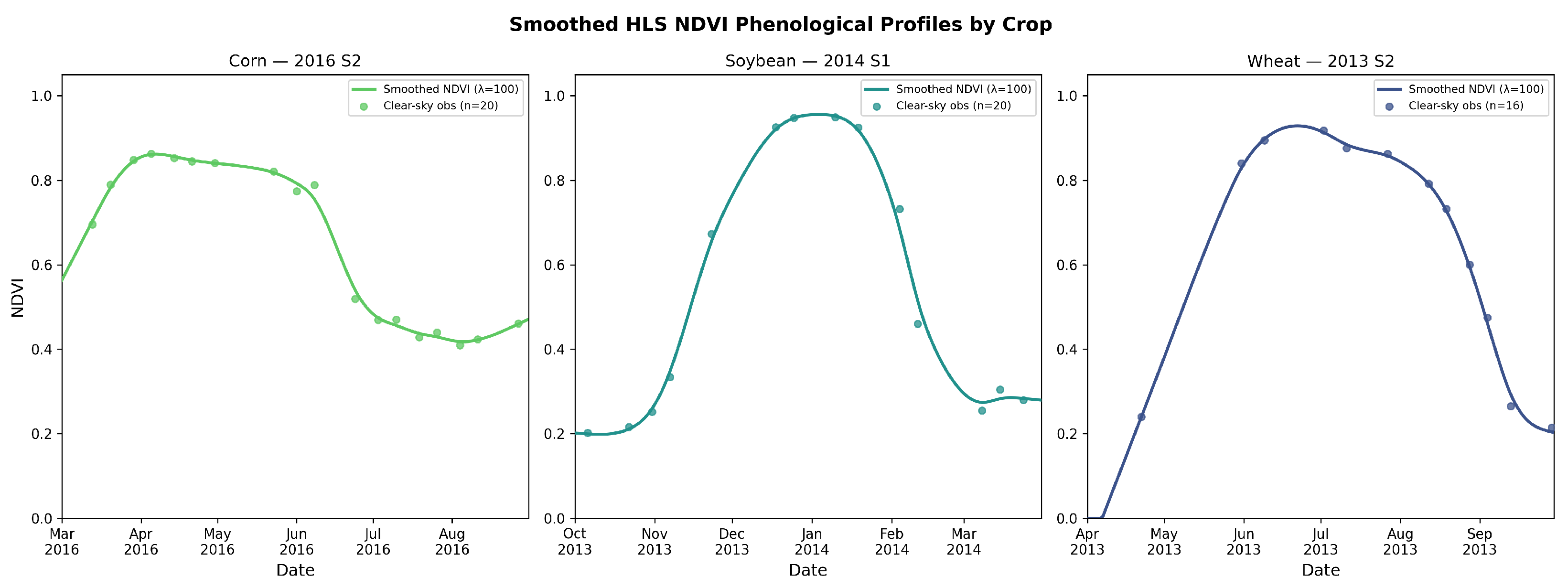
Figure 3 shows the smoothed HLS NDVI time-series for one representative growing season per crop, constructed from the raw clear-sky acquisitions in the Earth Engine export files. Cloud and shadow contamination was identified using the same NDVI saturation threshold applied in the main pipeline (NDVI $\ge 0.99$ flagged as cloud-affected); the Whittaker smoother ($\lambda =100$) then reconstructed a continuous daily curve from the remaining clear-sky observations. Each panel shows the actual irregular spacing of HLS acquisitions, which reflects the combined revisit frequency of Landsat-8 and Sentinel-2 with cloud-cover losses removed.

The corn profile (2016 S2) shows a clear green-up from March, a peak around June at NDVI $\approx 0.86$, and a gradual senescence toward harvest in August. The soybean profile (2014 S1) starts low in October, rises sharply to a peak near 0.95 by December–January, then senesces rapidly through February–March, consistent with the fast crop cycle of tropical soybean varieties. The wheat profile (2013 S2) shows a slower build from April, a June peak near 0.92, and a decline to harvest in September. The higher peak NDVI and more pronounced seasonal amplitude in soybean and wheat, compared with corn, are consistent with the higher absolute MI scores for vegetation features in those crops.

3.3. Ablation Study: Effect of harvest_day_of_year

Table 4. Ablation study: best accuracy (%) with and without harvest_day_of_year. Unablated values include SVM (five algorithms); ablated values exclude SVM (four algorithms). $\Delta$ is the accuracy drop attributable to removing the feature.

Crop	Task	Unablated	Ablated	$\mathbf{\Delta }$
Corn	Three-class	56.7 (RF)	49.8 (RF)	−6.9
Corn	Binary	73.4 (GB)	73.5 (KNN)	+0.1
Soybean	Three-class	56.5 (RF)	48.4 (KNN)	−8.1
Soybean	Binary	78.9 (GB)	74.9 (GB/KNN)	−4.0
Wheat	Three-class	70.9 (KNN)	58.0 (RF/GB)	−12.9
Wheat	Binary	98.7 (all)	84.5 (GB/LR/KNN)	−14.2

summarizes the impact of removing harvest_day_of_year from the feature set. The ablation reported here removes only harvest_day_of_year; a group-level ablation that separately removes all vegetation or all climate features was not performed in this study and is recommended as a future extension to quantify the relative contribution of each feature group. The unablated column reports the best accuracy achieved by any algorithm with the feature included; the ablated column reports the best accuracy without it. For the binary wheat task, all five algorithms (including SVM) converged to 98.7% in the unablated configuration, a result indistinguishable across structurally different learning algorithms and therefore diagnostic of near-deterministic separation by a single feature rather than genuine model learning. Removing the feature reduced wheat binary accuracy to 84.5% (three algorithms) and wheat three-class from 70.9% to 58.0%. For corn and soy the drop is smaller, confirming that harvest_day_of_year contributed less signal to those crops. The ablated results are the ones reported and discussed throughout this paper.

3.4. Three-Class Classification Performance

Full results are in

Table 5. Model comparison: accuracy (%) and macro-averaged F1. Best per row in bold.

Crop	Task	RF	GB	KNN	LR	Dummy
Accuracy (%)
Corn	Three-class	49.8	49.7	48.8	43.6	33.4
Soybean	Three-class	47.4	47.5	48.4	45.7	33.3
Wheat	Three-class	58.0	58.0	52.3	53.4	33.3
Corn	Binary	72.5	73.4	73.5	61.7	66.6
Soybean	Binary	72.7	74.9	74.9	71.5	66.7
Wheat	Binary	72.8	84.5	84.5	84.5	66.7
Macro-averaged F1
Corn	Three-class	0.479	0.475	0.456	0.408	—
Soybean	Three-class	0.474	0.474	0.464	0.453	—
Wheat	Three-class	0.590	0.590	0.517	0.550	—
Corn	Binary	0.660	0.638	0.647	0.583	—
Soybean	Binary	0.663	0.659	0.662	0.653	—
Wheat	Binary	0.727	0.801	0.801	0.801	—

. For corn and soy, algorithm choice had little practical effect. All four fell within six percentage points (pp) for corn (43.6–49.8%) and within three pp for soy (45.7–48.4%). Wheat was more tractable; RF and GB both reached 58.0%, with LR and KNN trailing at 53.4% and 52.3%. The fact that LR is consistently the weakest for corn and wheat, but not dramatically so for soy, suggests the corn and wheat class boundaries are more non-linear, while soy’s very tight yield range produces boundaries that are almost as amenable to a linear model as to an ensemble.

Per-class reports for RF are in

Table 6. Classification Report—Wheat, RF, Three-Class.

Class	Precision	Recall	F1-Score	Support
Low	0.93	0.56	0.70	306
Medium	0.43	0.74	0.54	306
High	0.67	0.44	0.53	305

,

Table 7. Classification Report—Corn, RF, Three-Class.

Class	Precision	Recall	F1-Score	Support
Low	0.71	0.37	0.49	1160
Medium	0.48	0.30	0.37	1158
High	0.44	0.82	0.57	1159

and

Table 8. Classification Report—Soybean, RF, Three-Class.

Class	Precision	Recall	F1-Score	Support
Low	0.74	0.38	0.50	1022
Medium	0.38	0.66	0.48	1022
High	0.51	0.38	0.44	1021

. In every crop, the Medium class had the worst F1 score: 0.54 (wheat), 0.37 (corn), 0.48 (soy). This is not a model failure; it reflects the fact that Medium fields, by definition, sit between Low and High in the feature space, and many of them are spectrally indistinguishable from their neighbors.

3.5. Binary Classification Performance

Collapsing Medium into Not Low changed the picture considerably, particularly for wheat (Table 5 and

Table 9. Productivity ranges for binary classes (t/ha).

Crop	Class	Mean	Min	Max	Count
Corn	Low	5.66	0.86	7.18	4637
	Not Low	9.30	7.18	16.07	9268
Soybean	Low	2.99	0.50	3.67	4087
	Not Low	4.40	3.67	7.55	8171
Wheat	Low	0.58	0.34	1.16	1224
	Not Low	2.75	1.16	4.47	2448

,

Table 10. Binary classification report—Wheat, GB/LR/KNN (all 84.5%).

Class	Precision	Recall	F1	Support
Low	0.96	0.56	0.71	306
Not Low	0.82	0.99	0.89	612
Dummy baseline: 66.7%. RF: 72.8% (macro-F1: 0.727).

,

Table 11. Binary classification report—Soybean, GB (74.9%).

Class	Precision	Recall	F1	Support
Low	0.77	0.35	0.48	1022
Not Low	0.74	0.95	0.83	2043
Dummy baseline: 66.7%. KNN also 74.9%. LR: 71.5%. RF: 72.7%.

and

Table 12. Binary classification report—Corn, KNN (73.5%).

Class	Precision	Recall	F1	Support
Low	0.70	0.35	0.47	1160
Not Low	0.74	0.93	0.82	2317
Dummy baseline: 66.6%. GB: 73.4%, RF: 72.5% (above). LR: 61.7% (below).

).

The following paragraphs discuss binary performance crop by crop, in order of decreasing model accuracy.

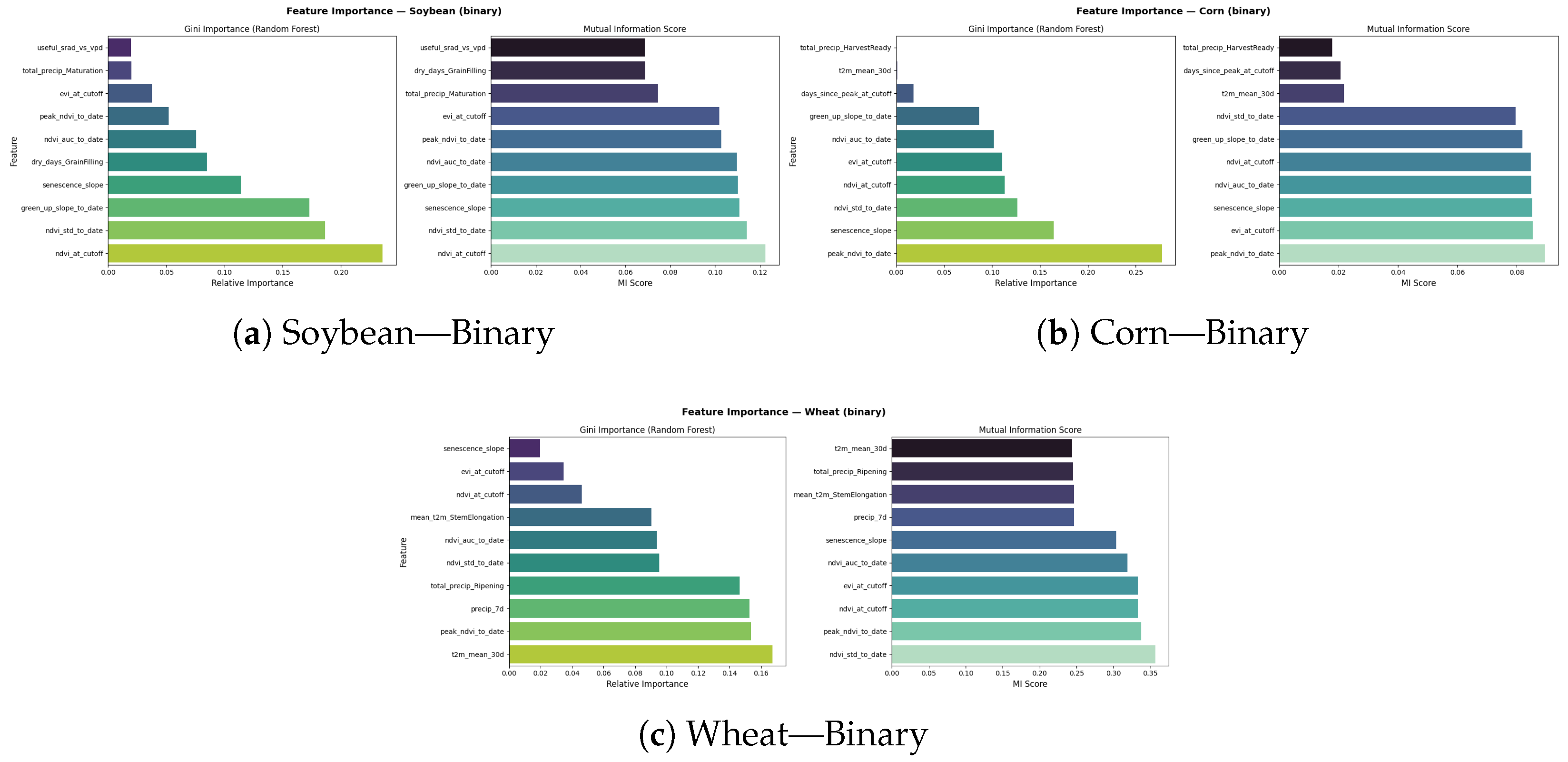
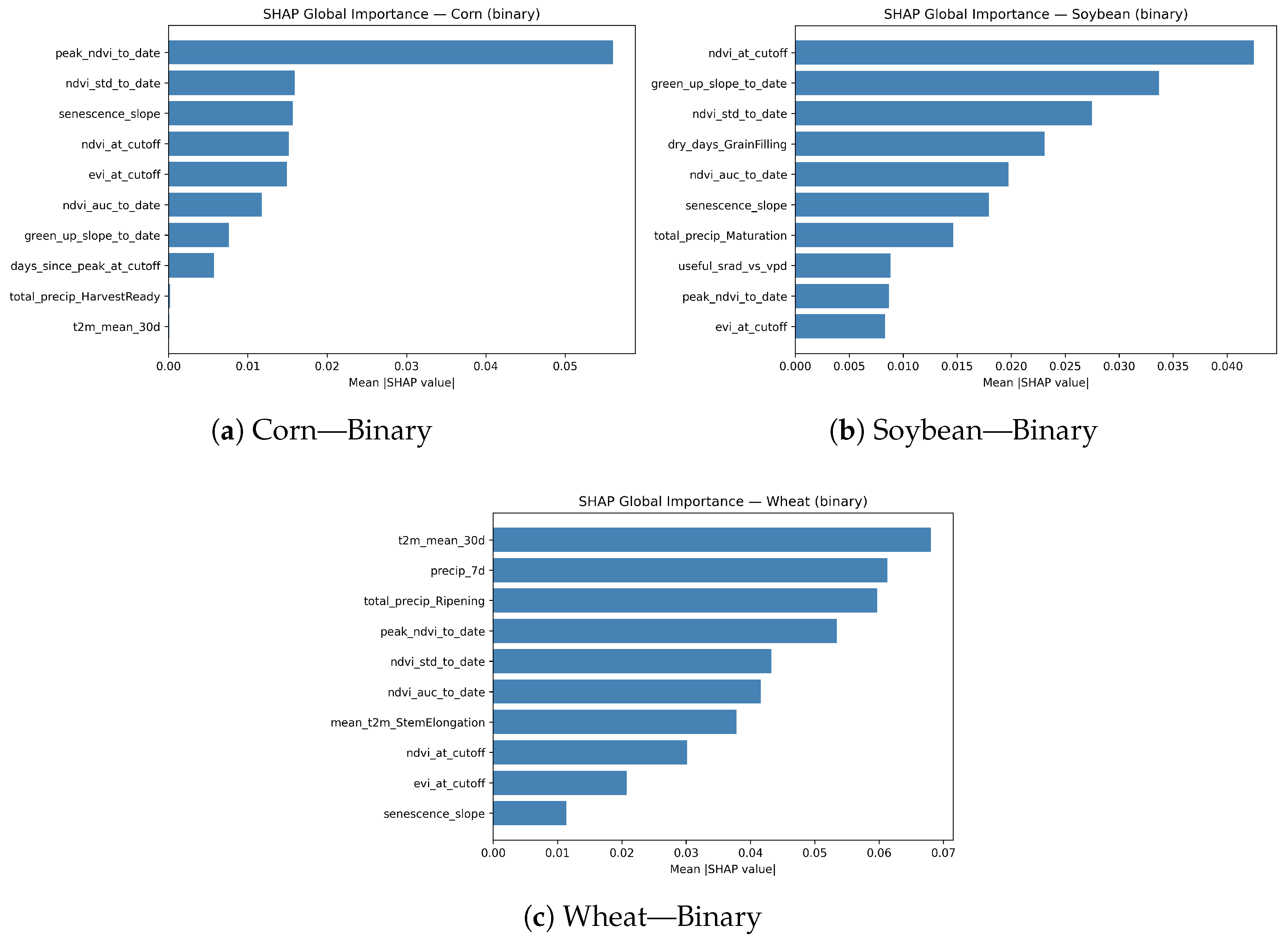
Wheat. GB, LR, and KNN all reached 84.5% (macro-F1: 0.801), 17.8 pp above the dummy baseline. RF reached 72.8%, with every error being a false positive and perfect Low-class recall. The fact that three structurally different classifiers converge to 84.5% using only pre-harvest vegetation and climate features is a key result: it suggests the remaining feature set contains a genuine, well-distributed signal for binary separation. In operational terms, 56% of genuinely at-risk wheat fields would be correctly identified (Low-class recall = 0.56), with a precision of 0.96, meaning very few false alarms. SHAP analysis of the binary RF model confirms that climate features are the primary drivers of risk detection: t2m_mean_30d (mean $\left|\mathrm{SHAP}\right|$ = 0.068), precip_7d (0.061), and total_precip_Ripening (0.060) are the top contributors, confirming that recent temperature and precipitation conditions close to harvest are the most informative signals for identifying at-risk fields. However, because all test-set seasons were drawn from the same farm complex and the same temporal pool as the training data, the model’s ability to generalize to unseen growing years has not been independently validated, and the results should be interpreted as showing application potential for yield risk early warning rather than confirmed deployment readiness.

Soybean. GB and KNN tied at 74.9%, with RF at 72.7% and LR at 71.5%. All four beat the baseline. GB’s Low-class precision of 0.77 versus RF’s 0.63 is consistent with the known behavior of boosting on imbalanced problems: sequential error correction keeps the model honest about ambiguous low-productivity cases that a parallel ensemble tends to classify with the majority.

Corn. Three algorithms beat the baseline: KNN at 73.5%, GB at 73.4%, RF at 72.5%. Only LR fell below at 61.7%. This is a meaningfully different result from the full-feature configuration, where only GB exceeded baseline. The vegetation feature set does contain signal for corn low-productivity detection, it was simply overwhelmed by harvest_day_of_year before. Low-class recall is still low across all models (RF: 0.43; GB: 0.33; KNN: 0.35), so most genuinely poor fields are still missed.

3.6. Confusion Matrices for Best-Performing Models

Table 13. Confusion matrix—Corn, RF, Three-Class.

	Pred Low	Pred Medium	Pred High
Actual Low	432	192	536
Actual Medium	153	352	653
Actual High	22	190	947

,

Table 14. Confusion matrix—Soybean, KNN, Three-Class.

	Pred Low	Pred Medium	Pred High
Actual Low	403	132	487
Actual Medium	114	265	643
Actual High	64	141	816

,

Table 15. Confusion matrix—Wheat, RF, Three-Class.

	Pred Low	Pred Medium	Pred High
Actual Low	171	135	0
Actual Medium	12	226	68
Actual High	0	170	135

,

Table 16. Confusion matrix—Corn, KNN, Binary.

	Pred Low	Pred Not Low
Actual Low	410	750
Actual Not Low	173	2144

,

Table 17. Confusion matrix—Soybean, GB, Binary (GB and KNN tied at 74.9%).

	Pred Low	Pred Not Low
Actual Low	359	663
Actual Not Low	106	1937

,

Table 18. Confusion matrix—Wheat, RF, Binary. RF achieves perfect Low-class recall (all 306 Low fields correctly identified) at the cost of 250 false positives, yielding 72.8% overall accuracy. This conservative behaviour is discussed as potentially preferable in insurance contexts where false negatives are costly.

	Pred Low	Pred Not Low
Actual Low	306	0
Actual Not Low	250	362

and

Table 19. Confusion matrix—Wheat, GB/LR/KNN, Binary. GB, LR, and KNN produced identical predictions (McNemar $b=c=0$), so a single matrix represents all three models.

	Pred Low	Pred Not Low
Actual Low	171	135
Actual Not Low	7	605

show confusion matrices for the best-performing model per crop and task. The matrices reveal misclassification patterns that aggregate accuracy metrics obscure. In every three-class task, the dominant error is misclassification toward the adjacent class: Medium fields are predicted as High for corn and soybean, and Low fields are predicted as Medium for wheat. The Medium class has the lowest within-class accuracy in all three crops, consistent with its position between Low and High in the feature space.

3.7. Bootstrap Confidence Intervals and Statistical Significance

Table 20. Bootstrap 95% confidence intervals for accuracy and macro-F1, best model per crop-task.

Crop	Task	Model	Acc (%)	Acc 95% CI (%)	Macro-F1 95% CI
Corn	3-class	RF	49.8	[48.2, 51.5]	[0.463, 0.496]
Soybean	3-class	KNN	48.4	[46.8, 50.1]	[0.447, 0.482]
Wheat	3-class	RF	58.0	[55.0, 61.4]	[0.560, 0.623]
Corn	Binary	KNN	73.5	[72.0, 74.8]	[0.629, 0.664]
Soybean	Binary	GB	74.9	[73.3, 76.4]	[0.638, 0.678]
Wheat	Binary	GB	84.5	[82.1, 86.7]	[0.771, 0.829]

reports bootstrap 95% confidence intervals (CIs; 1000 resamples) for accuracy and macro-F1 for the best-performing model per crop and task. The CIs confirm that the performance differences between crops are substantive: the wheat binary model (GB: 84.5%, CI [82.1, 86.7]) is clearly separated from the corn and soy binary models. Within each crop, CIs for the top models overlap, consistent with the McNemar test results discussed below.

McNemar tests on paired predictions confirm that for the three-class tasks, differences between the top models (RF and GB) are not statistically significant for corn ($p=0.78$) and soybean ($p=0.92$), consistent with the view that both models are operating near the same feature-imposed ceiling. All McNemar tests used the mid-point correction (Edwards’ correction) implemented in statsmodels.stats.contingency_tables.mcnemar. For wheat three-class and wheat binary, RF and GB produced identical predictions ($b=c=0$); in these cases the test statistic is undefined under the standard formulation. We report $b=c=0$ as evidence of complete agreement rather than a formal p-value. For wheat three-class, RF and GB are significantly better than LR ($p<0.001$) and KNN ($p=0.003$). For the binary tasks, GB and KNN are statistically indistinguishable for soybean ($p=0.86$) and for corn ($p=0.79$), while both are significantly better than LR ($p<0.001$). For wheat binary, the three top models (GB, LR, KNN) again produced identical predictions ($b=c=0$), and all three are significantly better than RF ($p<0.001$).

3.8. Spatial Distribution of Errors

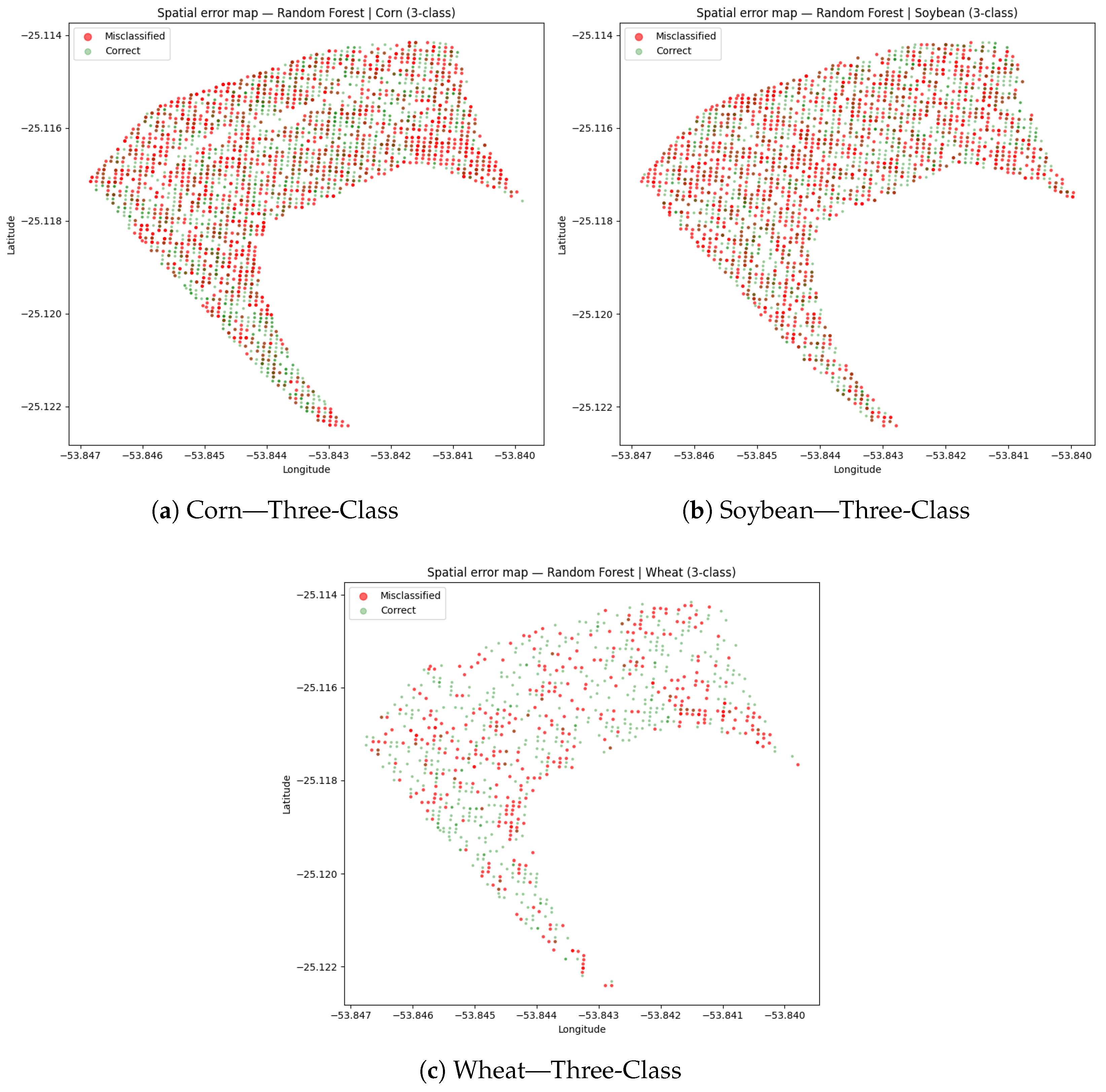
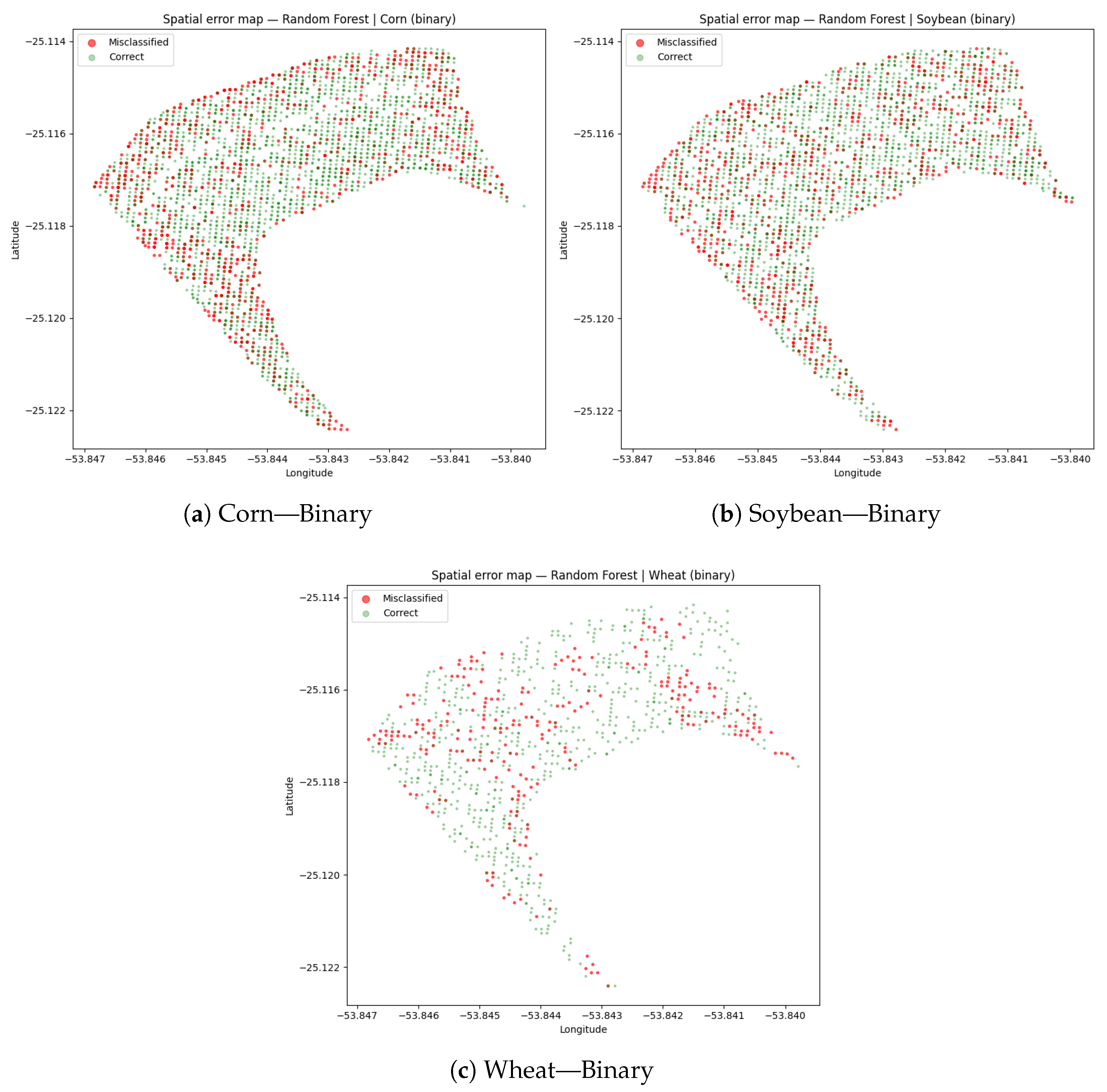
Figure 4 and Figure 5 show the spatial distribution of correct and misclassified grid cells for the RF model in the three-class and binary tasks, respectively. For corn and soybeans, misclassifications are distributed across the entire study area without obvious spatial clustering, suggesting that the dominant source of error is inter-annual variability in yield response rather than persistent spatial patterns such as field-edge effects. For wheat, the smaller dataset (two seasons) and higher overall accuracy produce sparser error maps; the misclassified cells do not cluster spatially, which is consistent with the strong spectral and climate signal identified in the feature importance analysis. The absence of strong spatial clustering in all cases provides some evidence that the errors are not caused by a single unobserved spatially structured covariate, though this interpretation is limited by the fact that the study area spans only approximately 25.6 ha and all cells are spatially contiguous.

3.9. Feature Importance and Selection Analysis

Removing harvest_day_of_year changed the importance profiles substantially. Rather than one feature absorbing half the model’s attention, the remaining predictors share importance more evenly, and the pattern differs between crops in ways that are agronomically interpretable.

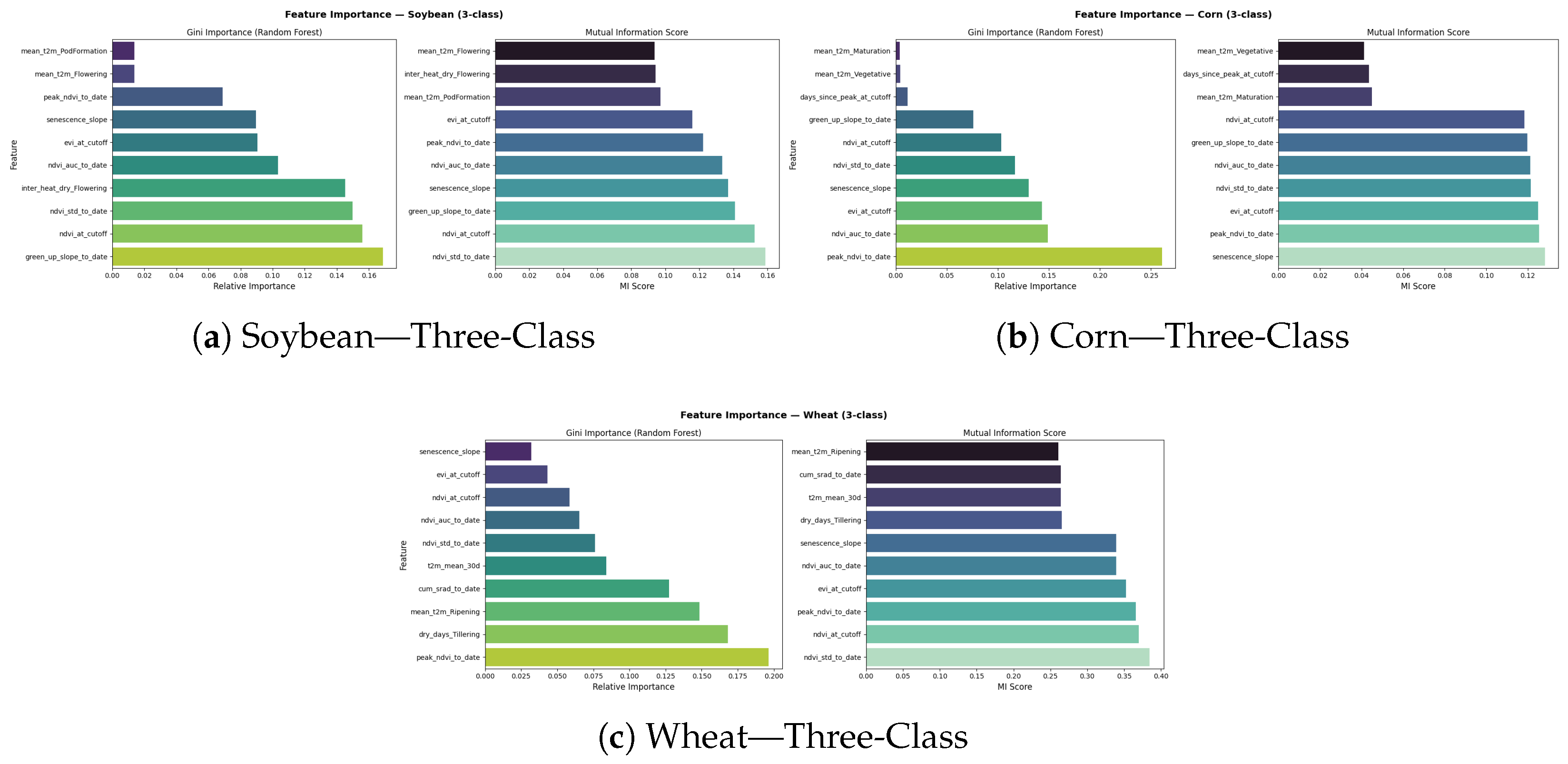
For corn, senescence_slope leads the MI ranking (0.128), with the top seven features nearly indistinguishable, ranging from 0.119 to 0.128: peak_ndvi_to_date (0.126), evi_at_cutoff (0.125), ndvi_std_to_date (0.121), ndvi_auc_to_date (0.121), green_up_slope_to_date (0.120), and ndvi_at_cutoff (0.118). Temperature features appear in positions 8–10 with substantially lower scores. The flat distribution says something important: no single spectral metric captures the dominant stressor in corn, which is consistent with the modest accuracy.

For soybean, NDVI features again lead, but temperature during reproductive stages enters the top-10 more clearly than for corn: mean_t2m_PodFormation (0.097), inter_heat_dry_Flowering (0.094), and mean_t2m_Flowering (0.094) all appear. Soybean is known to be sensitive to heat stress during flowering and pod-fill; these features reflect that sensitivity. In the binary soybean model, dry_days_GrainFilling (0.069) and total_precip_Maturation (0.075) also enter the top-10.

For wheat, the picture is different in two ways: the absolute MI scores are higher (ndvi_std_to_date: 0.384; ndvi_at_cutoff: 0.370; peak_ndvi_to_date: 0.366), and specific climate stages appear in positions 7–10 (dry_days_Tillering: 0.265; t2m_mean_30d: 0.264; cum_srad_to_date: 0.264; mean_t2m_Ripening: 0.261). For a winter cereal, vernalization, stem elongation, and grain-fill climate conditions are known to be decisive for final yield, so the presence of tillering and ripening features at high MI scores is expected. The higher informativeness of the wheat feature set is the most direct explanation for why wheat models outperform corn and soy models.

Gini importance from the RF models tells a consistent story. For corn (three-class), peak_ndvi_to_date takes 26.1% of total impurity reduction, followed by ndvi_auc_to_date (14.9%) and evi_at_cutoff (14.3%). Before ablation, a single feature had taken 59.8%. For wheat (three-class), peak_ndvi_to_date leads at 19.6%, with dry_days_Tillering (16.8%) and mean_t2m_Ripening (14.9%) close behind. The binary wheat model distributes importance across t2m_mean_30d (16.7%), peak_ndvi_to_date (15.4%), and precip_7d (15.3%), a stark contrast to the 61.8% single-feature dominance of the unablated version.

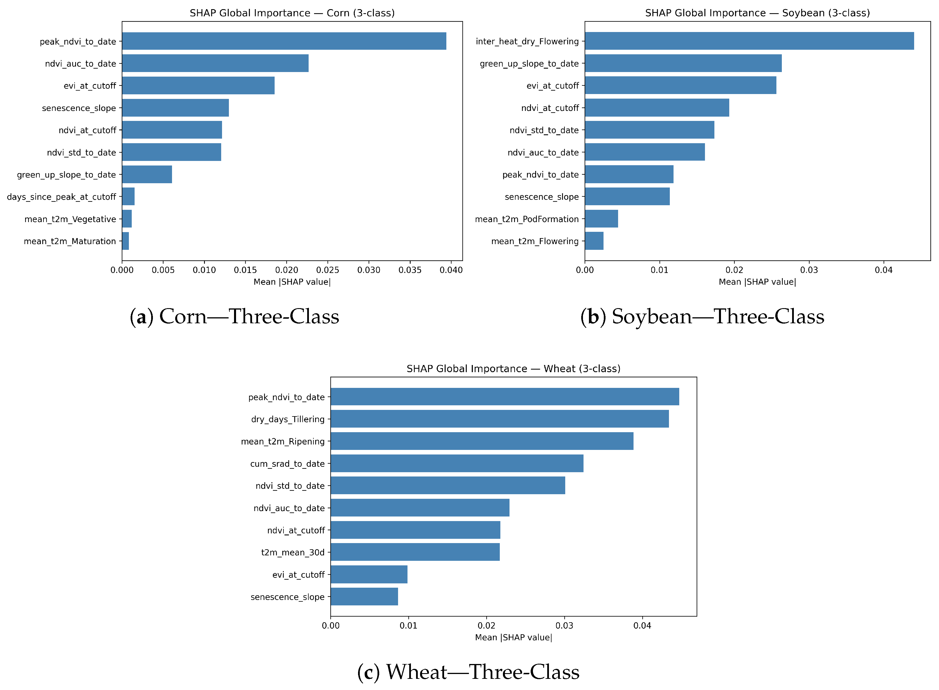
Feature rankings are shown in Figure 6 and Figure 7. Given that NDVI and EVI are derived from the same reflectance measurements and are therefore correlated, particularly at high canopy densities, the Gini importance rankings for these features should be interpreted collectively as spectral greenness indicators rather than as strictly independent predictors. MI scores are computed marginally between each feature and the target variable and are therefore not directly affected by inter-feature correlation in the same manner as impurity-based measures. For corn and soy, the MI and Gini top-five rankings share four or five of the five features across all four crop–task combinations. For wheat, the two methods diverge more within the top five: MI heavily favors NDVI-derived features globally, while Gini places climate-stage features higher because the RF exploits them more at split time. Both methods agree on the same 10-feature pool; they differ on internal ordering within it. Across all six crop-task combinations, SHAP, Gini, and MI consistently identified the same dominant feature groups, supporting the overall robustness of the feature selection results despite the presence of correlated predictors. A formal feature ranking stability analysis across cross-validation folds was not performed in the current study and is recommended for future work. To complement the Gini and MI rankings, SHAP (SHapley Additive exPlanations) values were computed for all RF models using a TreeExplainer. The mean absolute SHAP values are reported alongside Gini and MI scores in

Table 21. Top-five features by mean $\left|\mathrm{SHAP}\right|$, Gini importance, and MI score for the three-class RF model, per crop. SHAP values reflect the mean absolute contribution per prediction averaged across all classes; Gini and MI values are the same as reported in the feature importance analysis.

Crop	Feature	Mean $\left|\mathbf{SHAP}\right|$	Gini	MI
Corn	peak_ndvi_to_date	0.039	0.261	0.126
	ndvi_auc_to_date	0.023	0.149	0.121
	evi_at_cutoff	0.019	0.143	0.125
	senescence_slope	0.013	0.131	0.128
	ndvi_at_cutoff	0.012	0.103	0.118
Soybean	inter_heat_dry_Flowering	0.044	0.145	0.094
	green_up_slope_to_date	0.026	0.169	0.141
	evi_at_cutoff	0.026	0.090	0.116
	ndvi_at_cutoff	0.019	0.156	0.152
	ndvi_std_to_date	0.017	0.150	0.159
Wheat	peak_ndvi_to_date	0.045	0.196	0.366
	dry_days_Tillering	0.043	0.168	0.265
	mean_t2m_Ripening	0.039	0.149	0.261
	cum_srad_to_date	0.033	0.128	0.264
	ndvi_std_to_date	0.030	0.076	0.384

for the three-class task. For corn, all three methods agree that peak_ndvi_to_date is the dominant predictor (SHAP: 0.039, Gini: 26.1%), with spectral accumulation and senescence features ranking close behind. For soybean, SHAP places inter_heat_dry_Flowering (0.044) at the top, a feature that combines heat stress and dry days during the flowering window; this is the most notable divergence from Gini (which ranks it fourth at 14.5%) and highlights that the heat-drought interaction during flowering has a concentrated effect on individual predictions that broad-average Gini importance underestimates. For wheat, SHAP, Gini, and MI broadly agree on the top features: peak_ndvi_to_date (SHAP: 0.045) and dry_days_Tillering (SHAP: 0.043) rank first and second across all three methods, confirming that peak canopy development and water stress at tillering are the primary drivers of wheat yield variation in this dataset. SHAP bar and summary plots for all crop-task combinations are shown in Figure 8 and Figure 9.

4. Discussion

The clearest finding in this study is that for corn and soy, algorithm choice is essentially irrelevant for three-class accuracy. All four models clustered within six pp, and no consistent ranking emerged across crops. This is not surprising in retrospect: when MI scores plateau after the seventh feature and the top predictors are near-identical in informativeness, no algorithm, however expressive, can extract a signal that is not there. For these crops, the path forward is better features, not better models.

The binary tasks show a different pattern. Algorithm choice matters more when the classification boundary is simpler: the gap between the best and worst model was 10–13 pp for corn and soy and 12 pp for wheat. GB and KNN consistently outperformed RF and LR in the binary setting, which is consistent with their known strengths. GB’s sequential error correction focuses attention on hard examples near the class boundary; KNN’s non-parametric nature makes it well-suited to the compact, evenly distributed feature space that results after ablation.

The Medium class was the dominant error source in every crop. Medium fields sit in the middle of the feature distribution almost by definition, and many of them are spectrally indistinguishable from their neighbors. Improving Medium-class accuracy would require features that more precisely resolve the portion of the yield spectrum where most fields lie, which is harder than resolving the extremes.

Wheat deserves particular attention because the results changed the most after ablation. The three-class accuracy dropped from 70.9% to 58.0%, which confirms that harvest_day_of_year was contributing roughly 12 percentage points to the earlier result. The binary result is more encouraging: 84.5% accuracy using only pre-harvest features, with the convergence of GB, LR, and KNN reflecting a genuinely strong and distributed signal rather than task degeneracy. RF’s lower accuracy at 72.8% with perfect Low recall is interesting: it appears the RF is flagging every ambiguous field as Low, while the other three algorithms use the distributed climate signal to make finer distinctions. Whether this conservative behavior is a feature or a bug depends on the operational context: if a missed low-yield field is more costly than a false alarm, RF may actually be the right choice.

Soybean’s 74.9% binary accuracy (GB, KNN) represents an 8.3 pp gain over baseline from vegetation and climate features alone. The reduction from the earlier 78.9% confirms a modest contribution from harvest_day_of_year, but most of the soy signal was already in the spectral and climate predictors. Three-class performance remains limited by canopy saturation [14]: once the canopy closes, NDVI and EVI lose sensitivity to yield variation. The highest-confidence errors across all models share similar spectral profiles despite belonging to different productivity classes in different seasons, pointing to inter-annual climate anomalies as the missing signal.

Corn’s binary result is arguably the most informative finding in the study, not because the accuracy is high, but because of what changed. With harvest_day_of_year present, only GB exceeded the dummy baseline. Without it, three algorithms do. The vegetation features were never useless for corn; they were simply invisible next to a feature that explained far more variance. Even so, Low-class recall of 0.33–0.43 means the majority of genuinely poor fields are still missed, and the corn binary model is not recommended for standalone risk detection at its current performance level. The error analysis is telling: the highest-confidence misclassifications have ndvi_auc_to_date ≈ 110 and peak_ndvi_to_date = 1.0 regardless of whether the field ended up Low or Not Low, which suggests that inter-annual climate variability not captured by the current feature windows is the likely source of ambiguity.

4.1. Value and Limitations of HLS Data Fusion

The use of HLS v2.0 addresses one of the most common practical obstacles in field-scale crop monitoring: cloud-induced data gaps. By combining Sentinel-2 MSI and Landsat-8 OLI observations into a single harmonized surface reflectance product, HLS substantially increases the number of clear-sky observations available per growing season compared with either sensor alone. The Whittaker smoothing applied to the clear-sky time-series successfully resolved all cloud-induced gaps in the final dataset, confirmed by zero missing values in the NDVI and EVI feature columns.

The HLS product is not without limitations. The harmonization process corrects for BRDF effects and differences in sensor spectral response, but residual inter-sensor differences may remain under thin cirrus conditions where the Fmask QA band may miss contaminated pixels. Red-edge bands available from Sentinel-2 are absent from Landsat-8, which prevented their use here; a Sentinel-2-only product would allow red-edge indices but at the cost of reduced cloud-free observation frequency.

4.2. Risk Assessment: Operational Considerations

The binary classification task was designed specifically as a pre-harvest risk assessment tool. The practical value of the model depends critically on the Low-class recall, that is, the fraction of genuinely poor fields that are correctly identified. This recall varies considerably across crops: wheat achieves 0.56 (GB/LR/KNN), soybean 0.35 (GB), and corn 0.33–0.43. These values mean that a meaningful fraction of at-risk fields will be missed in every crop, which limits the model’s utility as a standalone risk certificate but does not preclude its use as a triage tool that concentrates scouting and management resources toward the most likely problem areas.

The risk threshold is defined from the training distribution rather than from an agronomic or economic benchmark such as a break-even yield, making the risk signal relative rather than absolute. The single-site scope means that risk thresholds and feature importances are calibrated to the specific conditions of western Paraná and may not transfer directly to other regions without re-calibration. Temporal validation limitations are discussed in Section 4.4.

4.3. Practical Implications

For wheat, the ablated binary model shows strong application potential for yield risk early warning. It relies on features observable before harvest and achieves 84.5% accuracy with a 17.8 pp gain over the dummy baseline, with importance distributed across three independent predictor groups (vegetation, temperature, precipitation). In practical terms, an agronomist could run this model three to four weeks before harvest by querying the HLS archive for the current season and the NASA POWER API for accumulated climate data, then generating a field-level risk map showing which fields are likely Low versus Not Low. Fields flagged as Low could trigger: targeted pre-harvest scouting to confirm the classification and identify the cause (disease, drought, lodging); early engagement with crop insurers to begin documentation; or re-allocation of drying and storage capacity to prioritize Not Low fields. The conservative RF configuration, which missed no Low fields at 72.8% accuracy, may be preferable in insurance or resource allocation contexts where false negatives are costly. The three-class model at 58.0% is less impressive but still practically useful for:

• Directing field scouting effort toward high-risk areas before problems become visible.
• Guiding variable-rate input applications based on expected yield tier.
• Supporting harvest logistics and storage planning.
• Providing objective evidence for crop insurance claims.

For soybean, GB or KNN at 74.9% is the recommended binary classifier. GB is preferable when false alarms are costly (precision = 0.77); KNN when balanced recall is the priority. At 74.9% overall accuracy and Low-class recall of 0.35, approximately one in three genuinely poor soy fields would be missed; this should be communicated clearly to any end user. The model is most useful as a triage tool that concentrates scouting resources, not as a definitive risk certificate. For corn, we do not recommend the binary model for standalone operational use. The 6–7 pp gain over baseline is real, but a recall of 0.33–0.43 for the Low class means the model misses more poor fields than it catches, and the false-negative cost in corn (where late corrective action is rarely possible) is high. The three-class corn model’s High-class performance (precision = 0.44, recall = 0.82) is more actionable: it identifies most of the top-yielding fields with reasonable precision, which is useful for storage planning and grain trader negotiations even if the risk-detection task remains unsolved.

4.4. Limitations and Future Directions

All data come from a single spatially contiguous study area of approximately 25.6 ha in western Paraná. Whether the models generalize to different cultivars, management practices, or geographic regions is an open question requiring multi-site validation. The corn dataset covers five seasons spanning non-contiguous years with contrasting planting windows, which limits the range of climate variability captured; expanding the season count is the highest-priority extension for corn within the remote-sensing-only framework. Most importantly, temporal generalization has not been validated: the models were tested on a held-out random 25% of grid cells drawn from the same seasons as the training data, not on a fully withheld growing year. A rigorous assessment of deployment readiness would require training on seasons up to year $t-1$ and evaluating on year t predictions blind to observed outcomes.

The wheat dataset covers only two growing seasons (2013 and 2014). While the binary results at 84.5% are encouraging, two seasons provide an insufficient basis for assessing inter-annual generalizability. The wheat models may have learned patterns specific to those two years rather than stable agronomic relationships, and any operational application would require validation on additional seasons before deployment.

The NASA POWER climate data used in this study have a native spatial resolution of approximately 0.5 degrees (∼50 km). Because the entire study area (approximately 25.6 ha) lies well within a single POWER grid cell, all grid cells in a given season receive identical climate values, and any microclimate differences within the study area are not captured. While this is consistent with common practice in field-scale crop modeling, it introduces uncertainty that is difficult to quantify without higher-resolution weather station data or statistical downscaling. Future work should compare NASA POWER inputs with on-site meteorological records or dynamically downscaled products to assess whether the spatial averaging biases specific climate features.

The role of harvest_day_of_year merits further investigation. Unusually early or late harvests in this region tend to coincide with below-average yields, but whether this reflects genuine crop physiology or proxies for planting date decisions cannot be determined without explicit planting records. If it is primarily a management proxy, then including it in a deployed model would make the model brittle to changes in farming practice.

On the methodological side, scalar feature summaries inevitably compress information that sequence-aware models (Long Short Term Memory (LSTM), Temporal Convolutional Networks) could recover from the raw time-series. Climate anomaly features, precipitation or temperature expressed as departures from long-term seasonal means, would directly address the inter-annual confusion in corn and soy. The tercile-based class definitions should be revisited using clustering algorithms or agronomic break-even thresholds, which would improve class separability and give the productivity tiers clearer economic meaning. Hyperparameter tuning should be revisited with a larger search budget or a more efficient strategy such as Bayesian optimization (e.g., Optuna), and MI-based feature selection should be nested inside each cross-validation fold to remove the current source of potential optimistic bias. A formal collinearity diagnostic (e.g., Variance Inflation Factor or Pearson correlation heatmap) followed by removal of highly correlated features would complement the SHAP and MI analyses and further strengthen the feature importance conclusions.

5. Conclusions

5.1. Main Findings

We developed and tested a grid-cell-scale crop productivity classification framework for corn, soy, and wheat in western Paraná, using harmonized Landsat/Sentinel-2 imagery and gridded climate data across 29,835 observations from 2560 unique 10 × 10 m grid cells. The central methodological finding is the identification and removal of harvest_day_of_year, a feature responsible for 47–64% of model importance and a spurious binary wheat accuracy of 98.7%. Removing it and re-running all models revealed the genuine discriminative capacity of the remaining pre-harvest feature set.

Without the dominant temporal feature: (1) three-class accuracy clustered within 6 pp across all algorithms for corn and soy (43.6–49.8% and 45.7–48.4%, respectively), confirming that feature quality, not algorithm choice, is the binding constraint; (2) wheat three-class accuracy reached 58.0% (RF, GB), with MI and Gini importance distributed meaningfully across vegetation and climate-stage predictors; (3) wheat binary accuracy reached 84.5% (GB, LR, KNN), confirmed by three structurally different algorithms as a genuine signal rather than degeneracy; (4) soy binary accuracy reached 74.9% (GB, KNN), driven by spectral and reproductive-stage climate features; and (5) corn binary classification revealed vegetation-based discriminative signal previously hidden by the dominant feature (KNN: 73.5%, GB: 73.4%, RF: 72.5%), though Low-class recall remains too low for reliable risk detection.

5.2. Practical Implications

The risk threshold used throughout this study is the training-set first tercile for each crop: a field predicted as Low has an estimated yield in the lowest third of the historical range observed in training. This is an operational definition, not an agronomic or economic one; anchoring it to break-even yields or regional benchmarks is a recommended extension. The wheat binary model shows the strongest result in the framework (84.5%, three algorithms), with generalizability validation on additional seasons required before operational deployment. Soybean reaches 74.9% binary accuracy and is usable as a triage tool, provided end users understand that approximately one in three at-risk fields will be missed. The corn binary model is not recommended for operational risk detection at its current performance level; its three-class High-class result (recall = 0.82) is more immediately actionable for harvest logistics planning.

5.3. Future Research Directions

Three extensions are most likely to improve performance: (1) expanding the number of growing seasons, particularly for corn and soybean, to capture a wider range of inter-annual climate variability and give the models more discriminative signal across productivity classes; (2) adopting field-level or year-blocked train-test splitting to obtain conservative, temporally and spatially unbiased performance estimates; and (3) replacing scalar feature summaries with sequence-aware architectures (LSTM, temporal CNNs) that can exploit the full daily time-series directly. A comparison of HLS observation frequency against single-sensor alternatives (Landsat-only or Sentinel-2-only) would also quantify the cloud-gap reduction benefit of data fusion and is recommended as a future addition. On the classification design side, replacing tercile-based class boundaries with agronomically or economically motivated thresholds would give the productivity tiers clearer operational meaning and likely improve class separability.

References

1. Benos, L.; Tagarakis, A.C.; Dolias, G.; Berruto, R.; Kateris, D.; Bochtis, D. Machine learning in agriculture: A comprehensive updated review. Sensors 2021, 21, 3758. [Google Scholar] [CrossRef] [PubMed]
2. Claverie, M.; Ju, J.; Masek, J.G.; Dungan, J.L.; Vermote, E.F.; Roger, J.C.; Skakun, S.V.; Justice, C. The harmonized Landsat and Sentinel-2 surface reflectance data set. Remote Sens. Environ. 2018, 219, 145–161. [Google Scholar] [CrossRef]
3. Inglada, J.; Vincent, A.; Arias, M.; Tardy, B.; Morin, D.; Rodes, I. Operational high resolution land cover map production at the country scale using satellite image time series. Remote Sens. 2017, 9, 95. [Google Scholar] [CrossRef]
4. van Klompenburg, T.; Kassahun, A.; Catal, C. Crop yield prediction using machine learning: A systematic literature review. Comput. Electron. Agric. 2020, 177, 105709. [Google Scholar] [CrossRef]
5. Wulder, M.A.; Roy, D.P.; Radeloff, V.C.; Loveland, T.R.; Anderson, M.C.; Dungan, J.L.; Masek, J.G.; Markham, B.L.; Pekel, J.F.; Scambos, T.A.; et al. Fifty years of Landsat science and impacts. Remote Sens. Environ. 2022, 280, 113195. [Google Scholar] [CrossRef]
6. Zhong, L.; Hu, L.; Zhou, H. Deep learning based multi-temporal crop classification. Remote Sens. Environ. 2019, 221, 430–443. [Google Scholar] [CrossRef]
7. Pelletier, C.; Webb, G.I.; Petitjean, F. Temporal convolutional neural network for the classification of satellite image time series. Remote Sens. 2019, 11, 523. [Google Scholar] [CrossRef]
8. Ienco, D.; Interdonato, R.; Gaetano, R.; Ho Tong Minh, D. Combining Sentinel-1 and Sentinel-2 satellite image time series for land cover mapping via a multi-source deep learning architecture. ISPRS J. Photogramm. Remote Sens. 2019, 158, 11–22. [Google Scholar] [CrossRef]
9. Lovelace, R.; Nowosad, J.; Muenchow, J. Geocomputation with R; CRC Press: Boca Raton, FL, USA, 2019; Available online: https://geocompr.robinlovelace.net/ (accessed on 1 March 2026).
10. Xue, J.; Su, B. Significant remote sensing vegetation indices: A review of developments and applications. J. Sens. 2017, 2017, 1353691. [Google Scholar] [CrossRef]
11. NASA Langley Research Center. POWER Project. Available online: https://power.larc.nasa.gov/ (accessed on 1 October 2025).
12. Embrapa. Tecnologias de Produção de Soja; Brazilian Agricultural Research Corporation (Embrapa Soja): Londrina, Brazil, 2020. [Google Scholar]
13. Licht, M.A.; Wright, K.; Coulter, J.A. Corn Growth and Development; University of Minnesota Extension: Saint Paul, MN, USA, 2021; Available online: https://extension.umn.edu/growing-corn/growth-and-development (accessed on 4 November 2025).
14. Maimaitijiang, M.; Sagan, V.; Sidike, P.; Daloye, A.M.; Erkbol, H.; Fritschi, F.B. Soybean yield prediction from UAV using multimodal data fusion and deep learning. Remote Sens. Environ. 2020, 237, 111599. [Google Scholar] [CrossRef]
Figure 1. Location of the study area. (A) Brazil in South America. (B) Approximate position of the study area (red star) in western Paraná. (C) Satellite image showing field boundaries.
Agriengineering 08 00203 g001
Figure 2. Data processing and machine learning workflow.
Agriengineering 08 00203 g002
Figure 3. Smoothed HLS NDVI time-series for one representative growing season per crop: corn 2016 S2 (March–August), soybean 2014 S1 (October 2013–March 2014), and wheat 2013 S2 (April–September 2013). Filled points are the mean NDVI across all sampling points on each clear-sky acquisition date. The continuous line is the Whittaker smoother (λ = 100) fitted to the irregularly spaced observations. The irregular spacing of acquisition dates reflects the combined Landsat-8 and Sentinel-2 revisit schedule after cloud masking.
Agriengineering 08 00203 g003
Figure 4. Spatial distribution of correct (green) and misclassified (red) grid cells, RF model, three-class task. No obvious spatial clustering is visible for any crop.
Agriengineering 08 00203 g004
Figure 5. Spatial distribution of correct (green) and misclassified (red) grid cells, RF model, binary task. For wheat, all Low cells are correctly classified by the RF (perfect Low-class recall, RF model only; GB/LR/KNN at 84.5% accuracy have Low-class recall = 0.56, as reported in Table 10); all RF errors are Not Low cells predicted as Low.
Agriengineering 08 00203 g005
Figure 6. Top 10 feature importances, three-class task (ablated). Left: Gini importance (RF). Right: Mutual Information score. Climate stage features (dry_days_Tillering, mean_t2m_Ripening) are prominent for wheat but absent from the corn and soy top-10.
Agriengineering 08 00203 g006
Figure 7. Top 10 feature importances, binary task (ablated). For wheat, importance is broadly distributed across temperature, vegetation, and precipitation features, contrasting with the 61.8% single-feature dominance in the unablated model.
Agriengineering 08 00203 g007
Figure 8. SHAP global feature importance (mean | SHAP | ), RF model, three-class task. Rankings are consistent with the MI and Gini orderings shown in Figure 6.
Agriengineering 08 00203 g008
Figure 9. SHAP global feature importance (mean | SHAP | ), RF model, binary task. Climate features dominate for wheat; vegetation features dominate for corn and soybean.
Agriengineering 08 00203 g009