


Abstract
Hyperspectral airborne data combined with machine learning has proven effective for characterizing plant nutritional quality. However, terrain, viewing geometry, and illumination can distort spectral signatures, leading to biased models with limited generalizability for large-scale mapping across farms with a heterogeneous landscape. In this study, we developed a framework for mapping pasture quality using airborne hyperspectral imaging while explicitly accounting for in-field acquisition and environmental effects. Nitrogen content (N%) and metabolizable energy (ME) were used as reference indicators across four hill country farms in New Zealand with contrasting environmental and management conditions. Ground truth was obtained using standard laboratory wet chemistry methods and paired with AisaFENIX airborne hyperspectral data, resulting in 1610 spectral samples derived from 161 spatially independent ground plots. Gaussian Process Regression (GPR) and a one-dimensional convolutional neural network (1D-CNN) were trained and evaluated on an independent test dataset. Both models achieved strong predictive performance (R2 > 0.8); however, GPR provided more reliable estimates through predictive uncertainty. Using a 95% confidence interval threshold to mask uncertain predictions increased overall performance (R2 > 0.9) and consequently improved the reliability of the mapped outputs. This approach enables spatially explicit pasture nutrient assessment to support precision land management for carbon and nitrogen.
1. Introduction
Grasslands are critical for maintaining sustainable ecosystem processes and provide multiple ecosystem functions [1,2] such as nutrient cycling and carbon sequestration [3,4]. The agricultural sector is highly dependent on managed grasslands (i.e., pasture) that sustain economic activities relying on these systems, e.g., nourishing livestock for dairy production [5,6]. In addition, pastures have a role in greenhouse gas (GHG) emissions and their management. For example, pasture quality influences GHG emissions such as N2O, which is generated through soil microbial nitrification and denitrification processes. On farms where fertilizer inputs and environmental conditions (e.g., rainfall and temperature) remain relatively stable, the main factor driving variation in N2O emissions is the amount of nitrogen excreted by grazing animals. This excretion is closely linked to pasture quality and the nitrogen content of the diet. High-quality, nitrogen-rich pastures increase urinary nitrogen excretion, providing more substrate for microbial transformation in the soil and ultimately leading to higher N2O emissions, while low-quality forage can elevate methane emissions due to less efficient digestion and longer rumen retention times [7,8,9]. Monitoring pasture quality is therefore critical for both economic and environmental sustainability. However, farms are complex systems, and pasture quality across a farm displays high spatial variability due to varying topography, geographical region, seasonal variability, changing climatic conditions, biodiversity, grazing, and land management [10,11]. This implies that farm-scale mapping is required to accurately estimate pasture quality in space and time [12,13].
Empirical modeling of site-specific data is often employed to estimate pasture quality and forage nutrients [14]. However, such data often consist of limited in situ point observations that may not capture farm-scale heterogeneity. In particular, linear regression models can be sensitive to multicollinearity among predictor variables, which may inflate uncertainty and reduce the reliability of coefficient estimates [15,16]. While increasing sample size can improve statistical power, collecting dense field samples at farm scale is costly and often impractical. Acknowledging these limitations, this study employs advanced machine learning approaches, specifically Gaussian Process Regression (GPR) and one-dimensional convolutional neural networks (1D-CNN), which are better suited to handle multicollinearity and complex, nonlinear relationships in high-dimensional hyperspectral data.
Remote sensing and, specifically, hyperspectral data could provide a scalable alternative by enabling high-resolution mapping of spatial variability across entire farms without the need for exhaustive ground sampling [17]. Ideally, spectral characteristics captured from the surface reflectance of the underlying surface (e.g., grass or canopy) can be used to estimate the biophysical and biochemical properties of plants. However, the radiation recorded by airborne or satellite sensors does not directly represent the true surface reflectance due to variations in atmospheric conditions (e.g., gas concentrations and aerosols), solar illumination geometry, and sensor viewing angles [18,19]. These directional effects are described by the Bidirectional Reflectance Distribution Function (BRDF), which defines how reflectance varies with illumination and observation geometry and is influenced by surface properties such as roughness and material composition [20,21]. While BRDF modeling can improve reflectance characterization, correcting for terrain-induced illumination effects requires additional topographic correction methods such as C-correction and Sun Canopy Sensor and C-correction [22,23,24,25]. These complex implementations (full BRDF and topographic correction methods) require detailed surface topography and multi-angular observations, posing computational and data-related challenges. Consequently, the implementation of directional and topographic effects is often not fully addressed in practice.
We hypothesize that advanced machine learning techniques can capture the complex relationship between reflectance data and plant nutritional properties (e.g., nitrogen content, metabolizable energy), even when the reflectance inputs lack full BRDF correction. By incorporating directional and environmental descriptors directly as model features, the learning algorithm can identify and compensate for these effects during training, reducing reliance on fully corrected reflectance products.
The overarching objective of this study was to develop a robust machine learning framework for predicting pasture nitrogen content (N%) and metabolizable energy (ME) in hill country farms from airborne hyperspectral data.
Leveraging a multi-farm, multi-environment dataset, we evaluated spectral sensitivity across the VNIR and SWIR regions and identified robust spectral ratios to reduce bias from variable illumination and moisture. Importantly, the proposed framework incorporates uncertainty quantification to support confident nutrient prediction across diverse agricultural landscapes and addresses key limitations in current hyperspectral nutrient mapping, especially reduced accuracy in complex terrain and limited generalizability.
2. Materials and Methods
The main objective of this study was to develop a robust and generalizable machine learning framework for predicting pasture nitrogen content (N%) and metabolizable energy (ME) using airborne hyperspectral data in New Zealand hill country farms. To achieve this, we pursued the following sub-objectives:
- Incorporate acquisition geometry (viewing and illumination angles) and environmental descriptors into the modeling process to account for directional and terrain effects.
- Evaluate the sensitivity of spectral features across VNIR and SWIR regions for predicting N% and ME.
- Identify spectral indices and band ratios that mitigate the influence of environmental variability (e.g., soil moisture, topography).
- Compare the performance of Gaussian Process Regression (GPR) and one-dimensional convolutional neural networks (1D-CNN) for nutrient prediction, including uncertainty quantification to improve model reliability and mask low-confidence predictions.
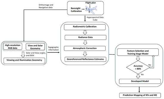
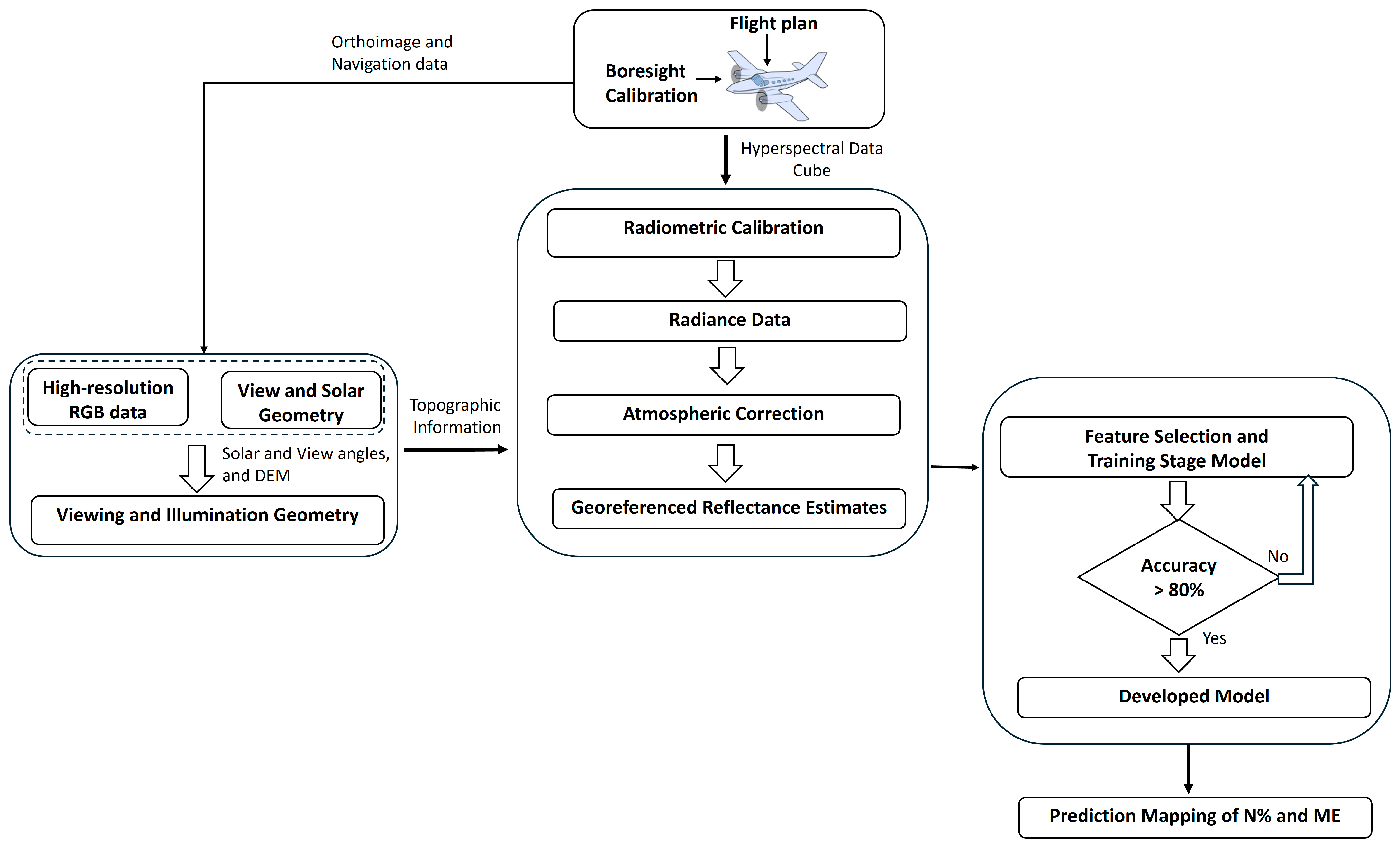
The framework for this work can be found in Figure 1, and further details are provided in Section 2.1, Section 2.2, Section 2.3 and Section 2.4.
Figure 1.
The framework followed during this study.
2.1. Study Area
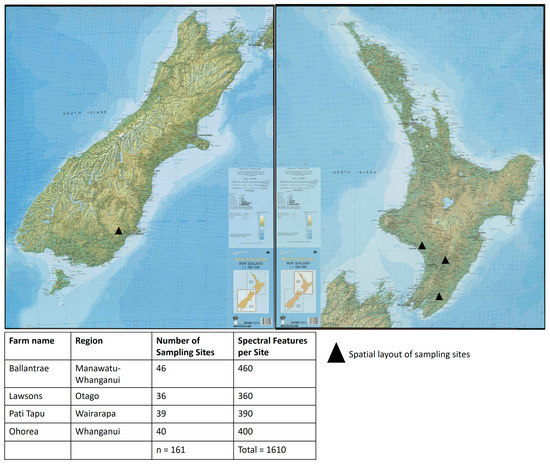
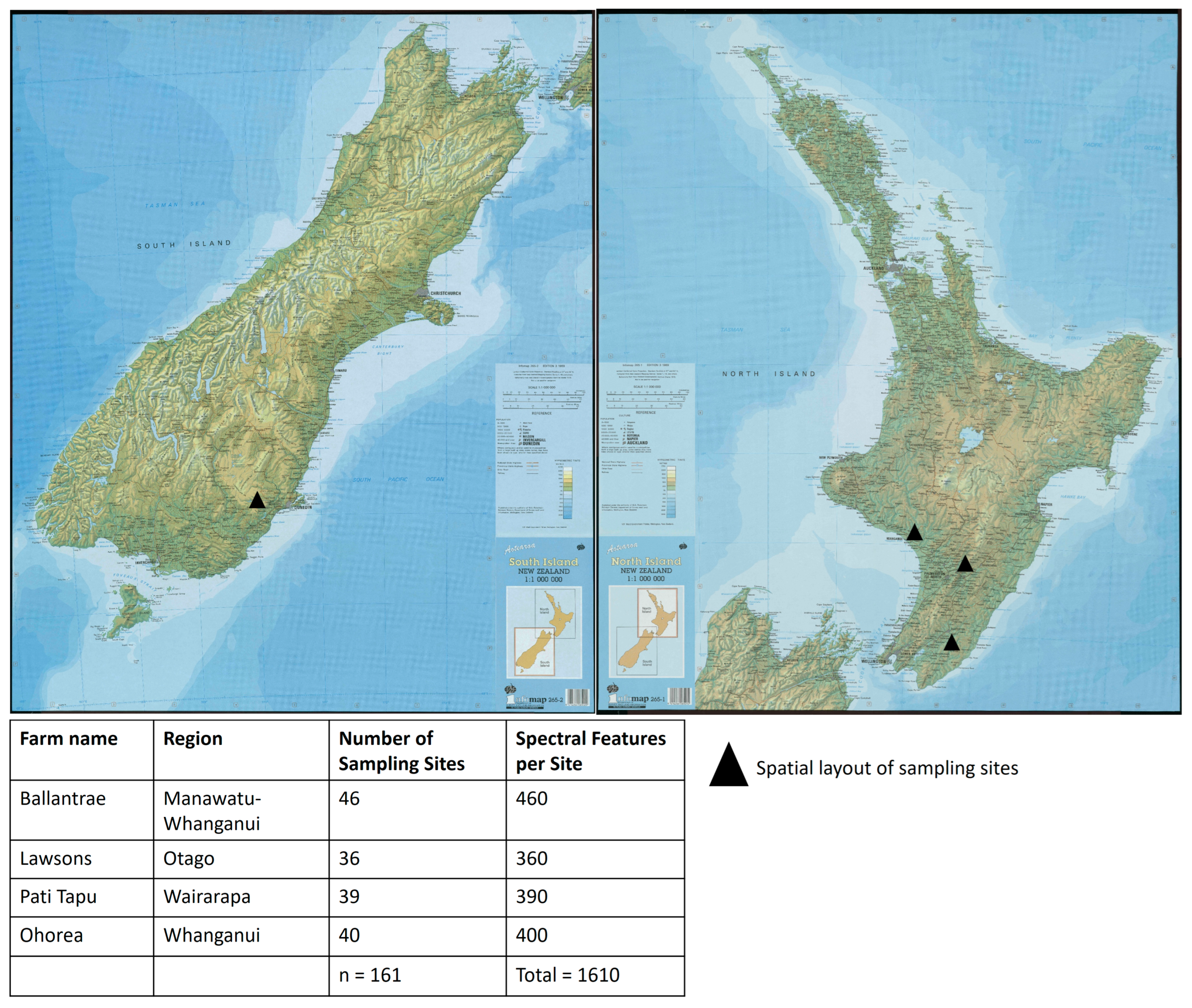
Four hill country farms were selected to capture a range of environmental conditions, topography, soils, hydrology, and management practices representative of New Zealand hill country pasture systems. Pasture species composition varies spatially within farms and can also change with phenological stage; for example, increased stem material during reproductive growth can reduce feed quality. Pastures at these sites are composed primarily of perennial ryegrass (Lolium perenne) and white clover (Trifolium repens), typical of New Zealand hill country, with variable contributions from other grass species depending on location and season. Because this characteristic alters reflectance signatures, it can be captured from hyperspectral data. Figure 2 summarizes the study locations and the number of sampling sites available for modeling.
Figure 2.
The map on the left displays the four Hill Country farms involved in this study. The corresponding number of ground samples collected from each farm is shown in the Table at the bottom.
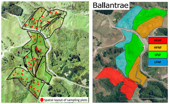
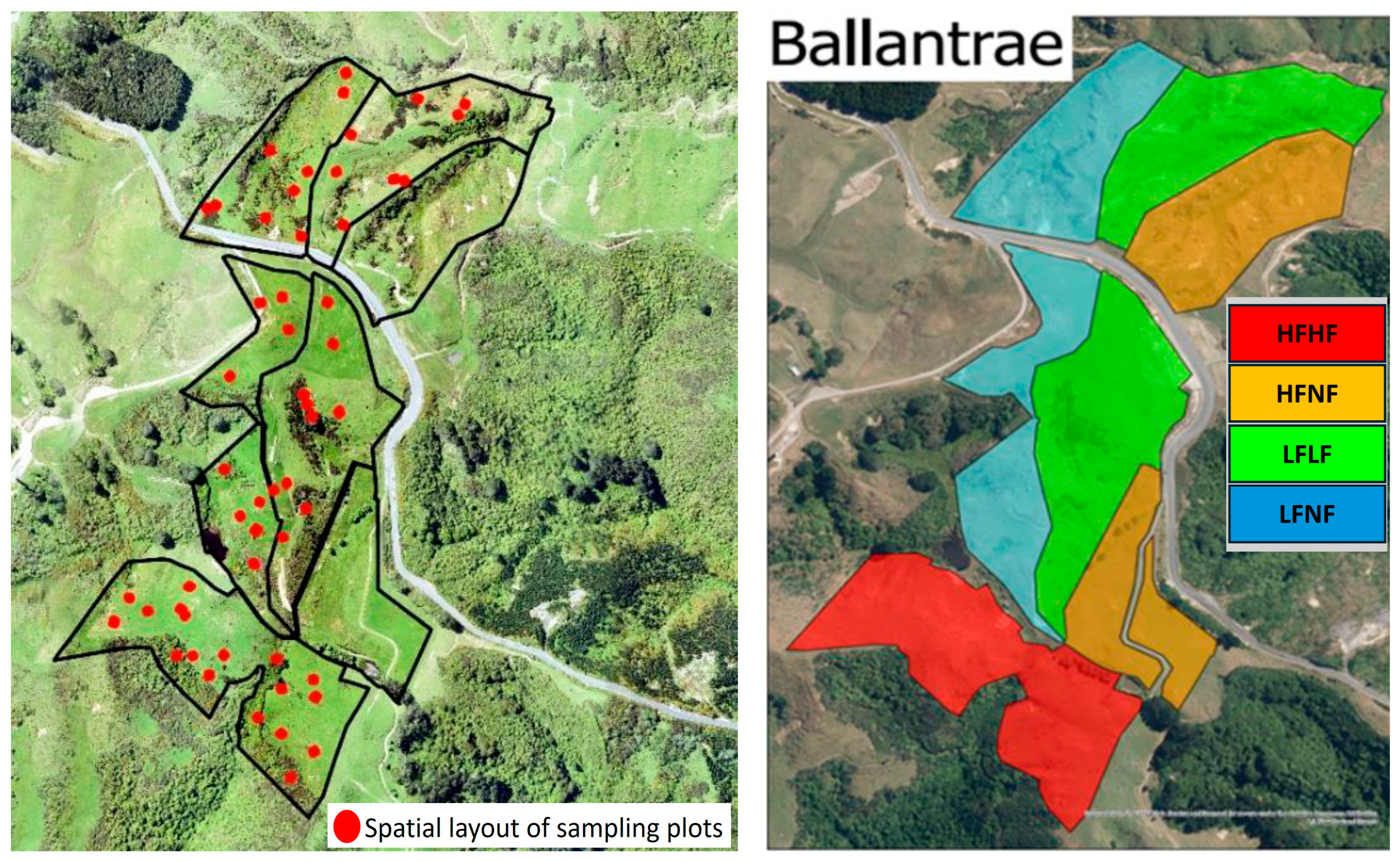
Ballantrae is a hard hill country farm in the Southern Hawke’s Bay region of New Zealand (40.30° S, 175.81° E) [26]. The Ballantrae farm is 125–350 m a.s.l. (above sea level) with an average annual air temperature of 12.8 °C and an annual rainfall of 1270 mm. The soils are of sedimentary origin, originally formed under forest. This farm was managed with a long-term fertility plan divided into four fertility zones (Figure 3). Each zone consists of 5–10 ha blocks; two blocks received low (LF) and two blocks received high (HF) fertilizer inputs between 1975 and 1980. Since 1980, fertilizer input has been withheld (no fertilizer (NF)) from one of the low (LF) and one of the high (HF) fertilizer blocks (LFNF and HFNF). By contrast, the other low fertilizer block (LFLF) has continued to receive 125 kg superphosphate (SSP)/ha/year and is stocked at 10.6 su/ha, and the other high fertilizer block (HFHF) has received 375 kg SSP/ha/year and is stocked at 16.0 su/ha.
Figure 3.
Ballantrae farm, with the fertility zone boundary shown in the (left) plot; the long-term fertility plan shows the HFHF, HFNF, LFNF, and LFLF zones on the (right). Pati Tapu is a 2200 ha farm 5 km south of Alfredton (40.75° S, 175.90° E) in the Northern Wairarapa (Figure 2) with approximately 30% valley floor flats and 70% hill country (with moderate to steep slopes in the north). The location of the farm is approximately 20 km east of the Tararua Ranges and 40 km from Castlepoint on the East Coast. The altitude is around 160–550 m a.s.l. Some summers can get very dry with an average annual rainfall of approximately 1050 mm. It is typical in the Wairarapa region for the majority of the rainfall to occur in the winter and spring, with unreliable summer rainfall. The average annual temperature is 18 °C.
Ohorea is a hill country farm (part of Ātihau-Whanganui Incorporation) at Waimarino 15 km south of Raetihi (39.53° S, 175.28° E), towards Whanganui (Figure 2), with a size of 5670 ha and approximately 1500 ha of non-productive (non-pasture) area. This farm has a mix of terrain with a large area of flat to rolling country. A large portion of the farm is a medium-to-steep hill, with some very steep faces along the Mangawhero River. The farm has a cool, high-rainfall climate. The average annual air temperature is 17 °C, and the annual rainfall is approximately 1300 mm.
Lawson farm is a 2336 ha hill country farm in East Otago, located approximately 30 km north of Dunedin (45.64° S, 175.58° E) (Figure 2). The farm is close to the coast, approximately 8 km inland from Karitane. The lowest parts of the farm are nearly at sea level, 20 m a.s.l., and the highest at 390 m a.s.l. A large area of the farm has flat regions and a hill country along the southeast boundary. Rainfall at this location varies from 750 to 1000 mm. The average annual air temperature is 20 °C.
2.2. Ground Measurements
In total, 161 spatially independent sampling plots were monitored (Figure 2), from which 1610 spectral samples were extracted. These were used for model training (n = 1127) and testing (n = 483). In addition, an independent validation dataset (n = 200) from the Ballantrae 2021 survey (exlusded from model training) was selected for model evaluation. A stratified random sampling approach was employed ensuring coverage of different slope classes and management zones across each farm. For each farm, ground measurements were randomly collected from 10 m × 10 m plots. The square plot design improves matching between ground sampling and aerial mapping and reduces sensitivity to GPS and co-registration errors. Sampling dates for each farm were as follows: November 2019 for Ohorea, November 2020 for Ballantrae and Pati Tapu, and November 2021 for Lawson. Sampling locations were georeferenced with RTK-GPS (Leica Viva GS16, Leica Geosystems AG, Heerbrugg, Switzerland). Within each plot, 95–100 grass clippings were collected to capture within-plot variability and were combined into a single composite sample to obtain one laboratory measurement per plot. All samples were cut to ground level using an electric shearing machine (Heiniger AG, Herzogenbuchsee, Switzerland) and transported in a cooling box for laboratory analysis. Dry matter was determined using standard drying (60 °C for 48 h). Total nitrogen (N%) was measured using the Kjeldahl method [27]. ME (MJ kg−1 dry matter) was derived from dry matter calorific value following the procedures described in [28,29].
2.3. Airborne Hyperspectral Data and Spectral Preprocessing
The hyperspectral data were collected using an AisaFENIX, Specim airborne hyperspectral sensor equipped with a GPS (GNSS/IMU navigation system (Specim, Oulu, Finland). The AisaFENIX sensor covers 377–2500 nm of spectral range in 449 spectral bands. The aircraft, with its ~32 degrees field of view, was flown at ~700 m height to scan the farm at 1 m2 spatial resolution. The hyperspectral data were collected within one to two weeks following the ground sampling. The raw sensor data (Digital Number (DN) values) were converted into radiance using the radiometric calibration from the 203 sensor’s gain and offset parameters. The radiance product is used to estimate surface reflectance, which captures the essential spectral characteristics of plant nutrients. Along with the hyperspectral camera, a Nikon DSLR (Nikon Corporation, Tokyo, Japan) camera was mounted on the same platform to capture high-resolution RGB data (spatial resolution of 3 cm). This high-resolution RGB was used to develop the Digital Elevation Model (using Pix4D desktop software, Available online: https://www.pix4d.com/product/pix4dmapper-photogrammetry-software/ (accessed on 6 January 2026) (Pix4D SA, Switzerland)) [30,31] and to develop a high-resolution RGB map of the farms for visual analyses.
For atmospheric correction, radiative transfer-based atmospheric correction was employed. The details of the radiative transfer-based atmospheric correction are given in [19,32,33,34,35]. To incorporate the viewing and illumination geometry in the atmospheric correction for each pixel, view-zenith and -azimuth angles, and solar angles were quantified using the planes’ navigation data. Further, atmospheric condition parameters—water vapor content and aerosol optical depth—were quantified using the methods given in [19,36]. To remove noise from the data that affects the model performance, the Savitzky–Golay (SG) was used [37,38].
2.4. Machine Learning Modeling
2.4.1. Data Preparation
Spectral data within each ground measurement plot (i.e., 10 m × 10 m plot used for ground sampling) were randomly sampled to obtain 10 spectral profiles from each plot. The spectral data were preprocessed to remove anomalies (e.g., sensor noise), and the actual ground measurements were used to label the N% and ME values for that plot. In total, 1610 spectral samples were extracted from the 161 ground plots, with each plot contributing 10 spectra to capture within-plot variability, out of which 1127 samples (70%) were used for model training, whilethe remaining 30% (n = 483) were used for model testing. In addition, an independent set of 200 samples was used for model evaluation.
2.4.2. Feature Selection
Kernel-based correlation metrics (Matern and squared-exponential kernels) combined with expert judgement were used to identify wavelengths containing non-redundant information related to N% and ME. A genetic algorithm (GA) was then applied to select a compact subset of informative predictors from the hyperspectral feature space [39,40]. Because hyperspectral data are inherently collinear, this two-stage selection reduced redundancy and improved model stability. Topographic and acquisition-geometry descriptors (e.g., illumination angle and view geometry) were included as additional predictors to capture residual terrain and illumination effects. In total, 43 predictors were selected from across the VNIR, NIR and SWIR regions and were standardized before modeling.
Further, for each selected wavelength/band, the spectral response function was utilized to guide the machine learning models to group the spectral bands from neighbouring wavelengths to enhance spectral information during the modeling stage. Spectral response functions (SRFs) describe the sensitivity of the sensor to neighbouring wavelengths to determine how much energy a sensor detects at each wavelength in the electromagnetic spectrum [41,42,43] and are commonly used in spectral super-resolution (pan-sharpening) [44,45]. We utilized the Gaussian response function and the sensor full width at half maximum (FWHM) to implement the SRF. For instance, if wavelength 650 nm was found to be sensitive to N% or ME, then a weighted average (Gaussian response function) of wavelengths from 630 to 670 nm was considered as the actual spectral value at 650 nm. This is in addition to the SRF implemented during the preprocessing stage to convert sensor-recorded data into physical units, such as reflectance.
2.4.3. Gaussian Process Regression (GPR) Modeling
We employed GPR modeling, which is a kernel-based machine learning algorithm and a state-of-the-art method to extract biophysical variables from spectral data [44,45]. A GPR assigns a probability distribution over a set of possible functions that fit the input data and converts them into posterior probabilistic estimates [46]. In general, GPR expresses predictive uncertainty, which is an essential attribute for maintaining confidence in the predictions [47,48,49]. Sources of uncertainty arise when the model is predicting from data independent from the training data. While data uncertainty occurs because of class overlap or due to the presence of noise in the data, estimating knowledge uncertainty is significantly more difficult than estimating data uncertainty [50]. Besides determining the confidence intervals around the predictions, we used the uncertainty information to mask non-pasture areas such as weeds, roads, or bare soil ground covers from the analyses. Because the training data used pasture spectral data only, predictions over non-pasture data should be biased. However, with a threshold, those classes can be masked.
The model hyperparameters were optimized using a gradient-based optimization algorithm that maximizes the marginal likelihood in the training data [51]. Because the GPR kernels have an impact on prediction accuracy, Matern, Squared Exponentials (RBF), Linear, ArcCosine, and Rational Quadratic kernels [52,53] were used.
2.4.4. One-Dimensional Convolutional Neural Network (1-D CNN) Modeling
The 1D-CNN architecture was implemented with Tensorflow in Python 3.10 as described by [54,55] and developed by [56]. To capture the nonlinearity in the data, the exponential linear unit (eLU) was used as the activation function between the layers, except for the last layer, which used a linear activation function. The weights on the multiple layers were initialized using the ‘HeNormal’ initialization and were trained using an adaptive moment optimizer algorithm (Adam). The mean squared error (MSE) was used as the loss. The maximum number of epochs allocated for the training process was 500. The training set was used for model calibration/training, and the test set was used for validation.
2.4.5. Accuracy Evaluation
The performance of each model was evaluated using the coefficient of determination (R2), normalized root mean square error percentage (nRMSE%), RMSE, mean squared error (MSE), and bias.
3. Results
3.1. Data Preprocessing and Feature Selection for Modeling
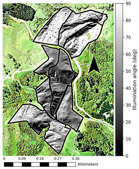
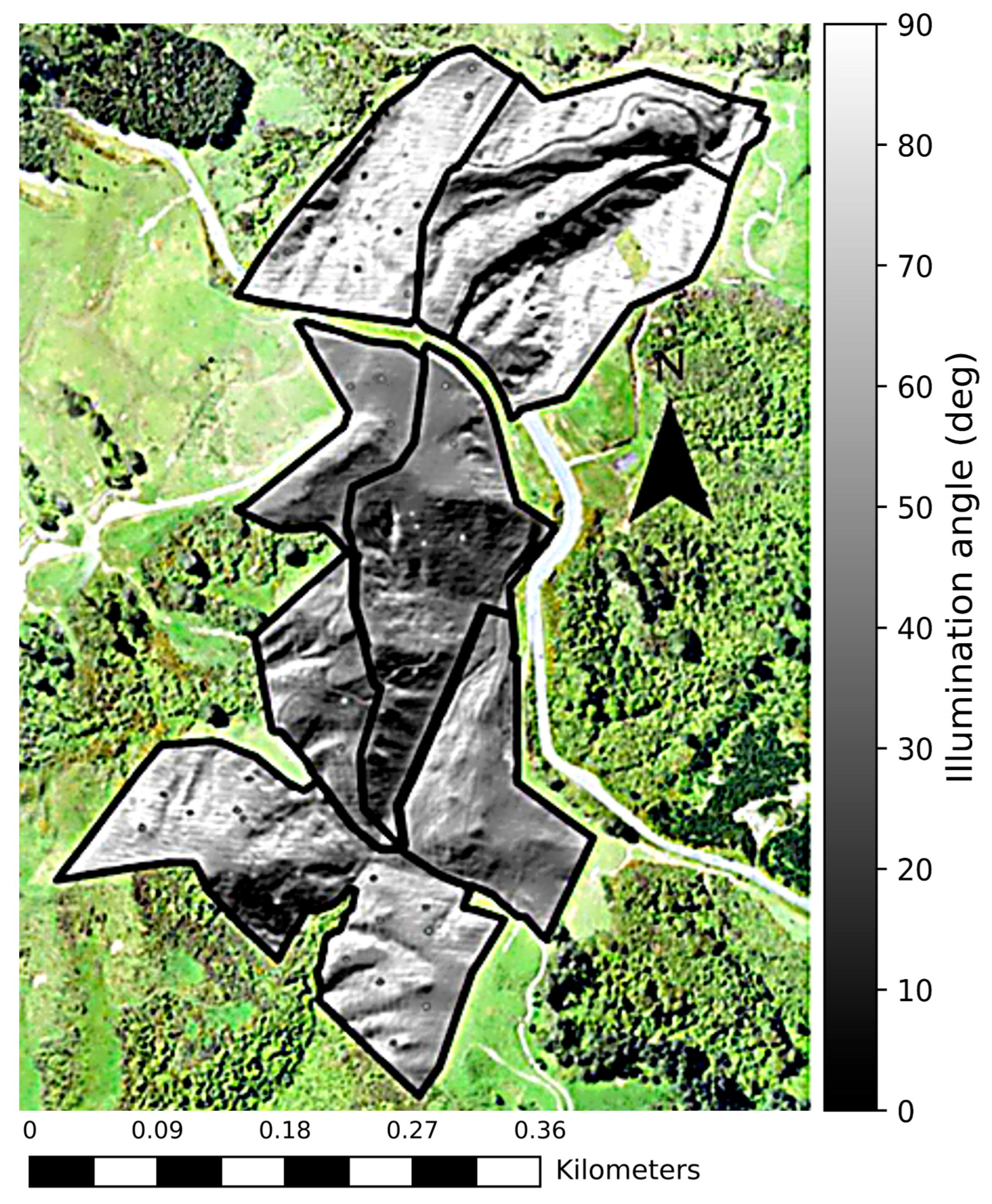
Airborne imagery exhibits geometric effects related to platform motion (roll, yaw, pitch) and terrain-induced variation in illumination and viewing geometry. For example, Figure 4 illustrates spatial variation in the derived illumination angle at the Ballantrae location. Consequently, reflectance processing incorporated platform geometry and solar angles during atmospheric correction to generate a terrain-aware reflectance factor product for each pixel, improving the consistency of reflectance values across heterogeneous landscapes.
Figure 4.
Illumination angle (between 0 and 90°) for each pixel is displayed. Variations in camera geometry, sun angle, and topography result in differing illumination effects, represented by varying shades of grey on the surface.
Wavelengths associated with N% and ME were identified through their associations with plant biochemical and biophysical properties and water content [57,58,59,60]. VNIR wavelengths capture pigment absorption and red-edge behavior, while SWIR wavelengths capture absorption features related to protein and water status.
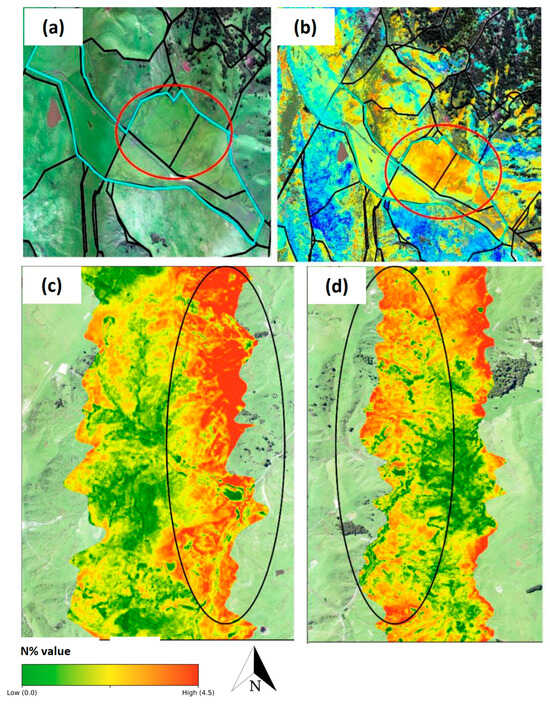
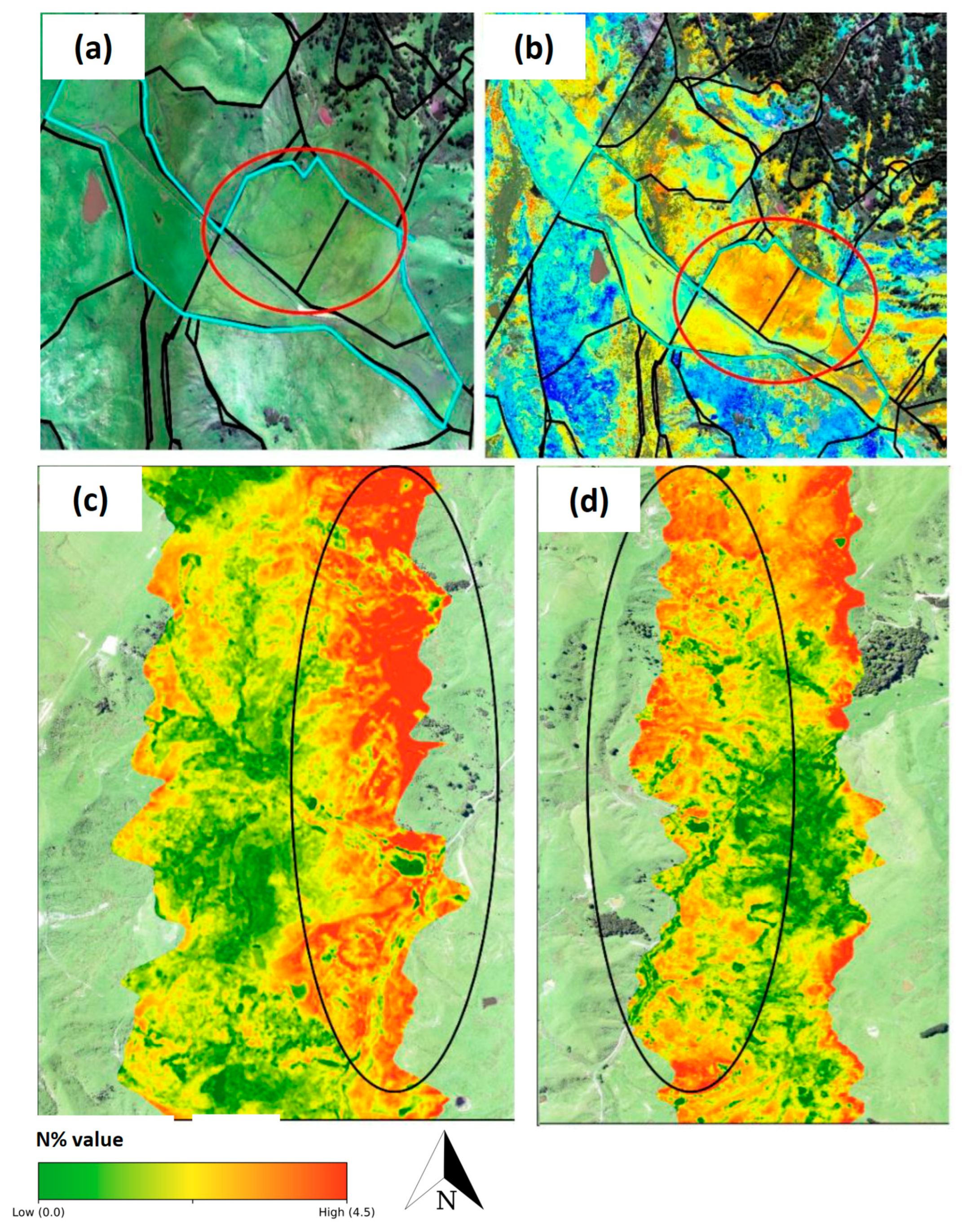
In the field, reflectance estimates are influenced by environmental factors (e.g., soil moisture and adjacency effects) and by view and illumination geometry. In the prediction maps, flat areas exhibited low nitrogen content (N% < 2.0), which is inconsistent with the ground measurements and general nutrient baseline of flat terrain, where N% and metabolizable energy (ME) are typically higher (N% > 3.0). However, we observed systematic underprediction in some downslope and flat areas (Figure 5a,b) and strip-to-strip differences between flight lines (Figure 5c,d).
Figure 5.
Maps in (a) show the flat areas of Ohorea farm (circled in red)—the general nutrient baseline of flat terrain—where N% and metabolizable energy (ME) are typically higher (>3.0%); areas where N% was underpredicted (<2.0%, in (b)) due to water content are highlighted. Maps in (c,d) show the strip effect (circled in black); because of different view and illumination geometry, the prediction of the same area is different in the North-to-South and South-to-North directions.
To reduce these effects, additional water-sensitive band ratios (e.g., around 890/965 nm, 1596/817 nm, and 855/1242 nm) were included as predictors, and illumination angle was included as a model feature.
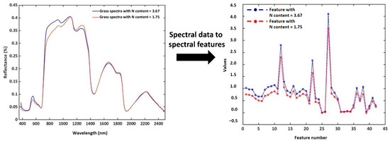
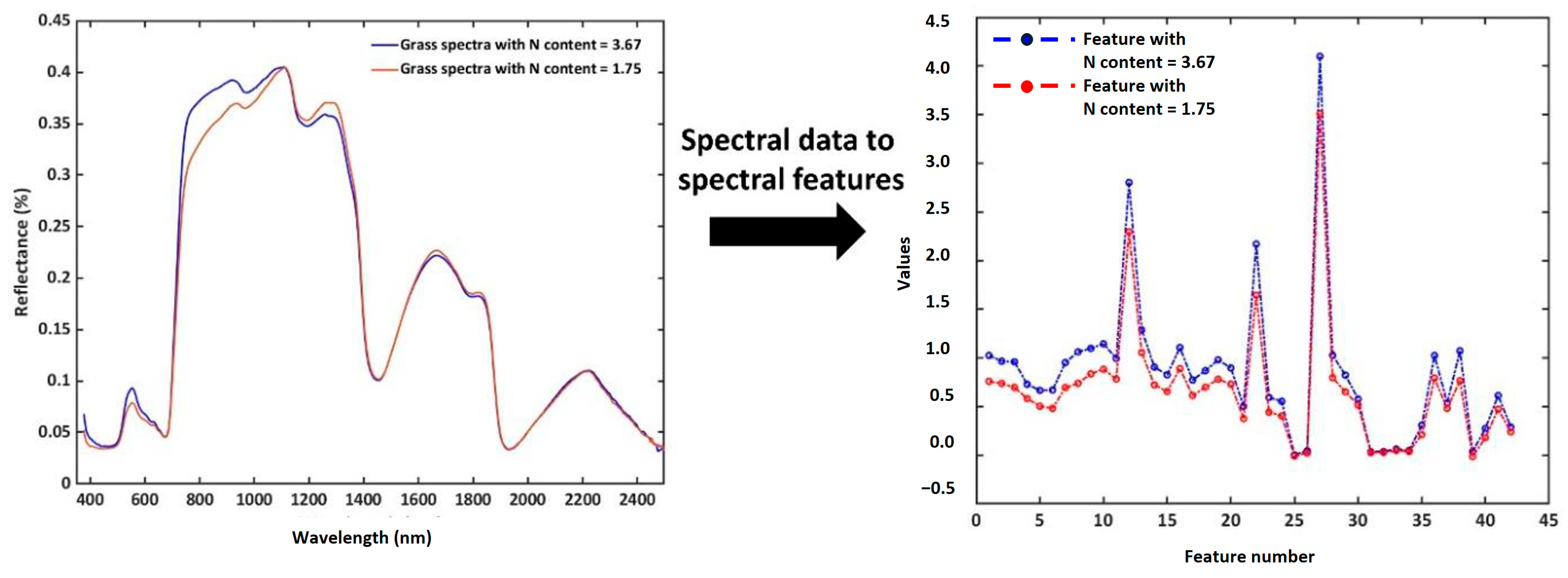
Wavelengths characterizing N% and ME are shown in Table 1. In total, 43 features were selected from these wavelengths (Figure 6). Data standardization was applied to these features before inputting them into the machine learning models to predict N% and ME.
Table 1.
Wavelengths characterizing plants’ biochemical and biophysical properties, N% and ME, and environmental conditions.
Figure 6.
Hyperspectral data are showcased on the left, and corresponding spectral features on the right.
3.2. Model Building with the Training Data
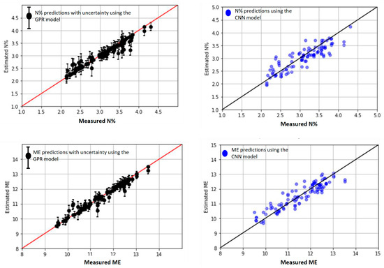
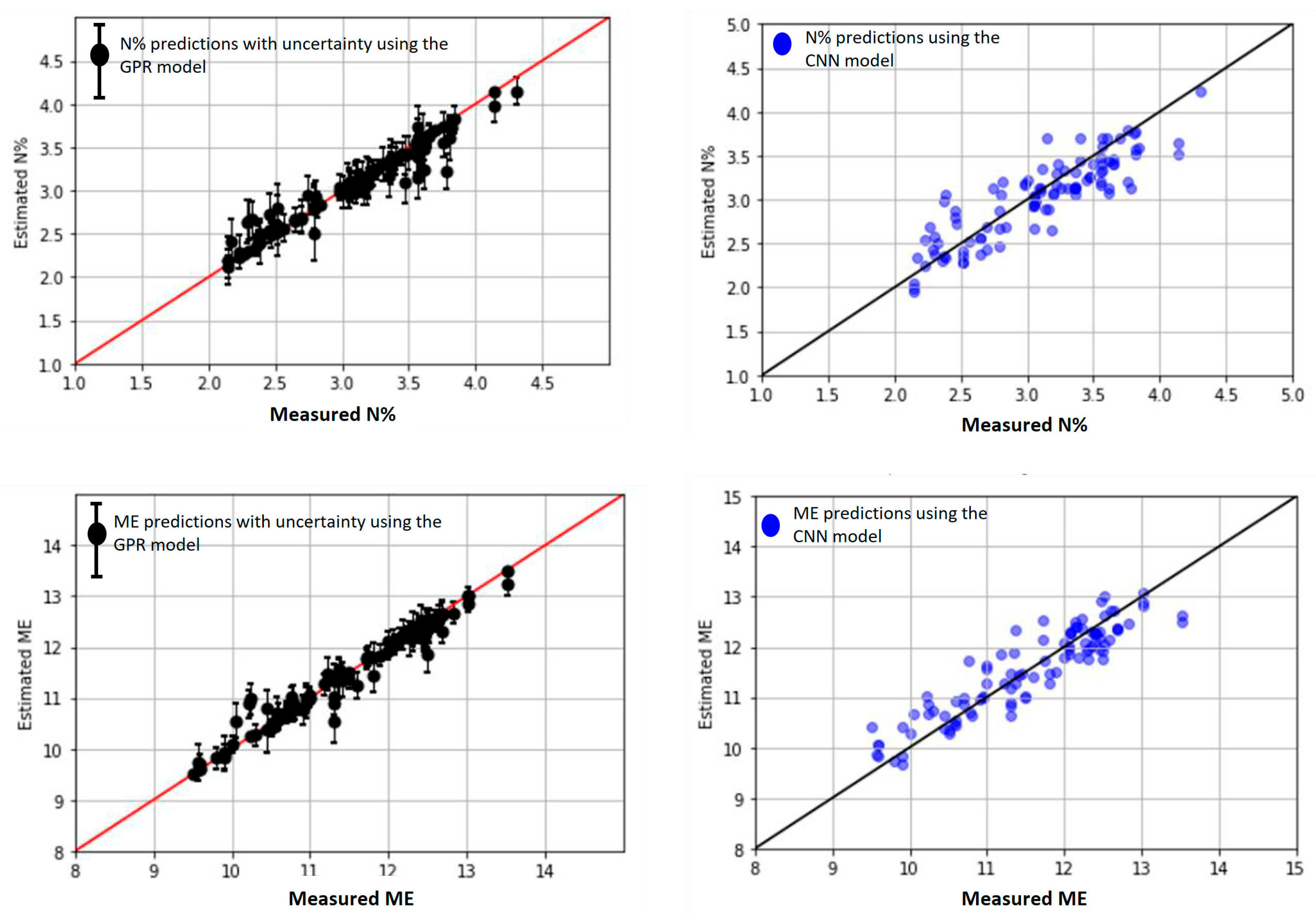
We found that for N% and ME predictions, the predicted values on the test data agreed best with the measured data when using the Matern family with (v = 1/2). Overall, the accuracy of the GPR model was better than that of the CNN model on the independent dataset (Table 2). This was further evidenced in the scatter plot of the measured versus predicted values for N% and ME (Figure 7).
Table 2.
Statistics of the GPR model and the 1-D CNN model.
Figure 7.
Scatter plot between the measured and predicted N% with the GPR model (top left) and the CNN model (top right). Scatter plot between the measured and predicted ME for the GPR model (bottom left) and the CNN model (bottom right). Performance data for each model can be found in Table 2.
3.3. Model Validation Using Independent Sampling Plots on the Ballantrae Farm
To evaluate model generalizability and prevent overfitting, an independent validation set was constructed using 20 additional plots (200 spectral samples) from the Ballantrae farm. These plots were surveyed during the November 2021 campaign but were not included in the training dataset. Ballantrae, being a long-term experimental site with well-characterized fertility zones and controlled management, provided an ideal setting for independent validation.
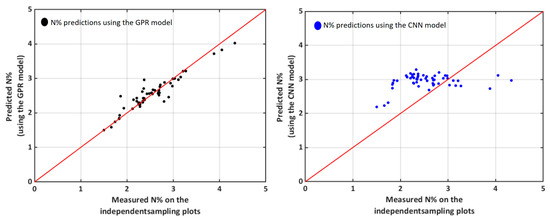
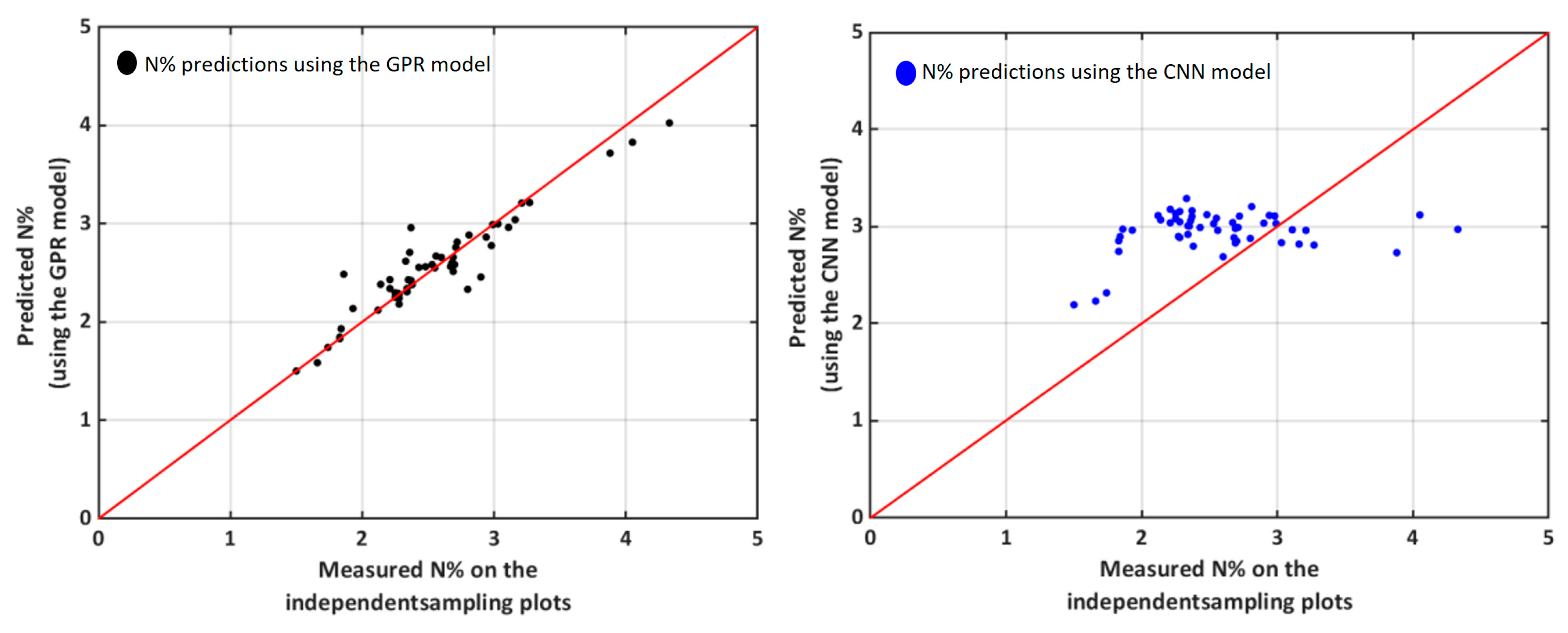
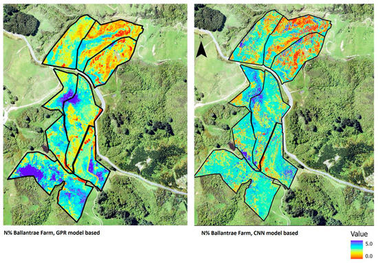
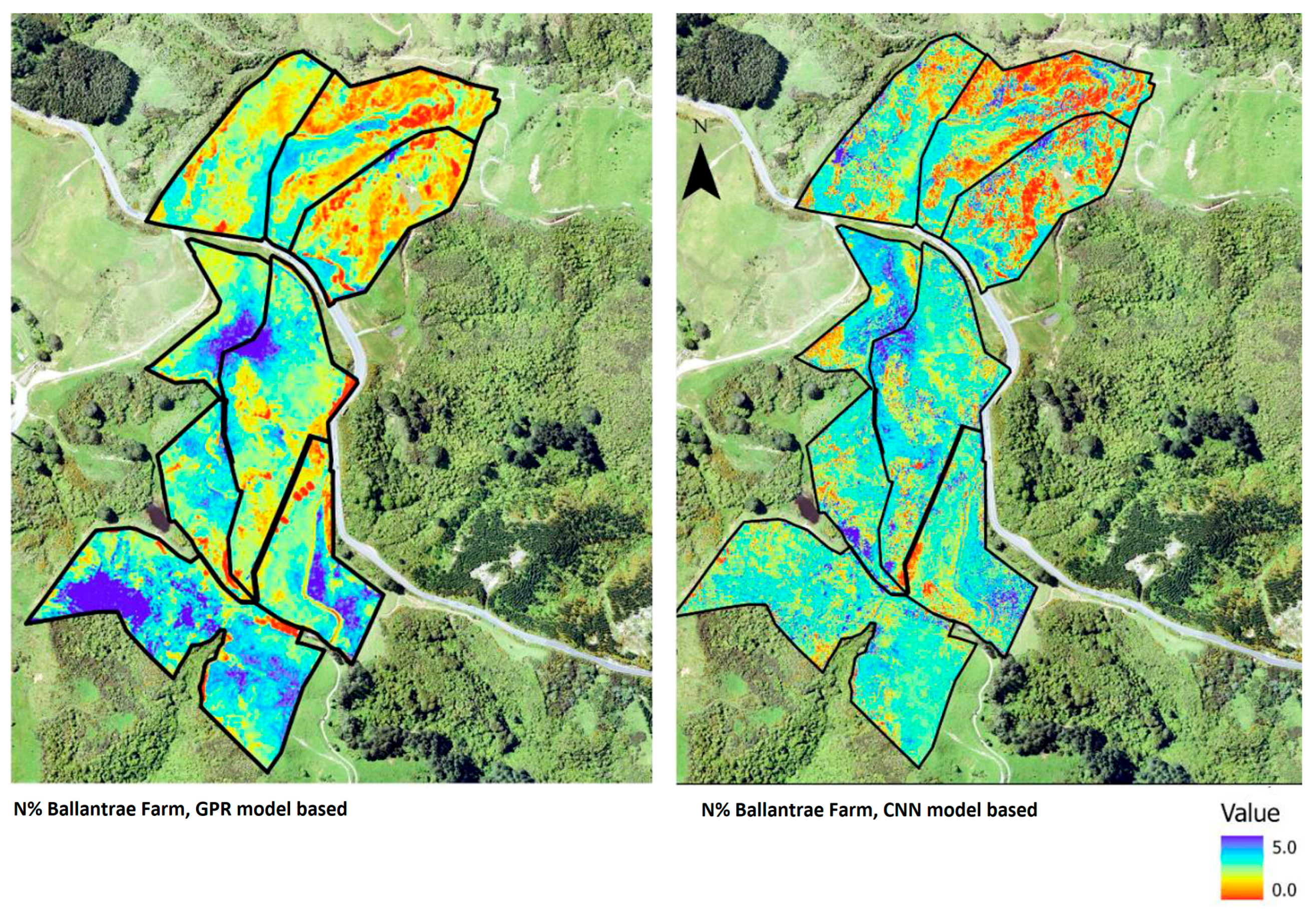
Because Ballantrae farm has long-term controlled fertility treatments, the values of N% and ME were expected to vary systematically across the different blocks. Specifically, higher values (N% > 2.5%) were expected in the HFHF due to sustained high fertilizer input, while reduced values (N% < 2.5%) were expected in the LFLF with lower nutrient input. Because Ballantrae serves as a controlled experimental site, the model was expected to capture these known fertility-driven trends in its predictions. The two models were employed to predict the N% and ME for each block of Ballantrae and were validated using the independent ground measurements of each block that were not included in the training datasets. The scatter plot of the measured vs predicted values is shown in Figure 8. The GPR model predicted N% well for most sampling locations, with R2 = 0.88 and RMSE = 0.17, except for two plots where over-prediction occurred. In contrast, the CNN model did not perform well, with (R2 = 0.07) and RMSE = 0.21 failing to capture the variation in the ground measurements. Consequently, the maps generated from the CNN model were inaccurate, as evidenced in Figure 9, e.g., N% was underpredicted in the high-fertility block.
Figure 8.
Scatter plot comparing measured and predicted N% values. (Left): GPR model, with R2 = 0.88 and RMSE = 0.17. (Right): CNN model, with R2 = 0.07 and RMSE = 0.21.
Figure 9.
Prediction results from the GPR model (left) and the CNN model (right) for all blocks in the Ballantrae farm.
3.4. Prediction Accuracy on All the Farms
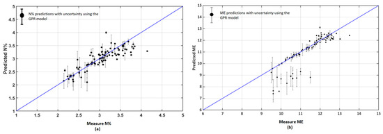
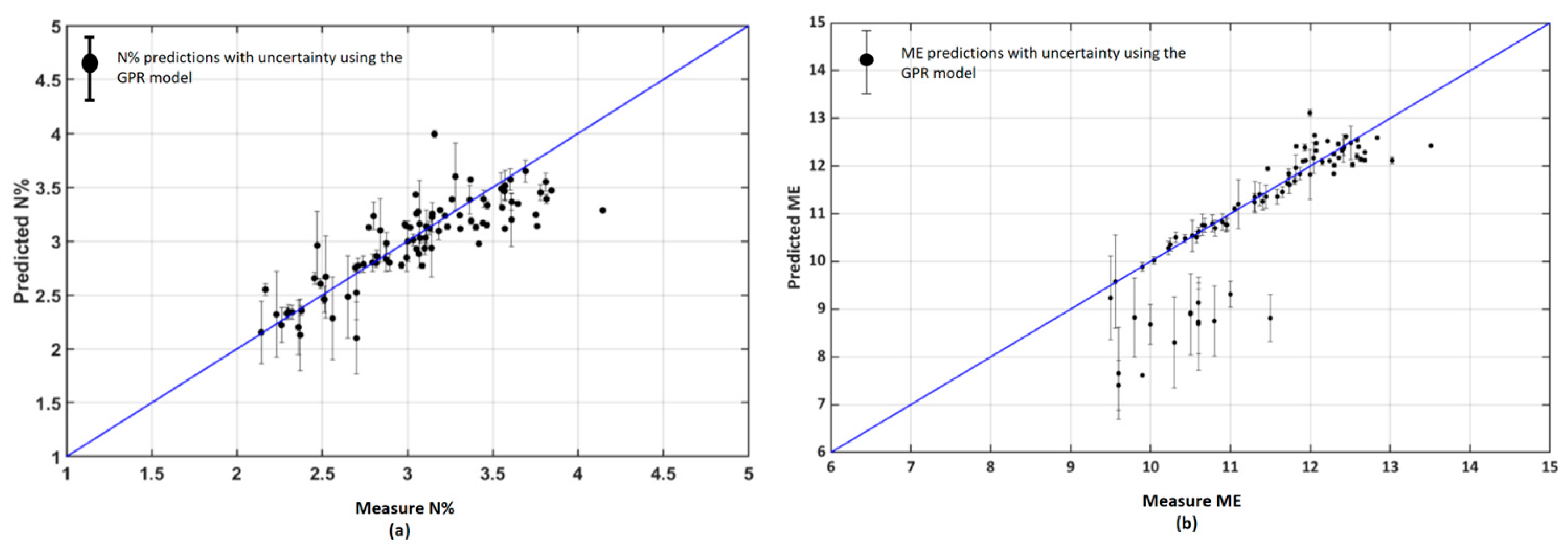
The GPR model had higher performance and was therefore selected. Model performance was estimated across all four farms, and prediction maps were generated. Figure 10 shows the predicted vs measured values for the N% content and ME for all four farms. The overall accuracy of the GPR prediction model was as follows: MSE = 0.050, RMSE = 0.228, nRMSE = 7.50, bias = −0.272, and R2 = 0.77 for N%. For ME, it was as follows: MSE = 0.284, RMSE = 0.533, nRMSE = 4.67, bias = −1.69, and R2 = 0.82.
Figure 10.
Scatter plot between the measured and predicted (a) N% and (b) ME for the four farms (with R2 ~ 0.8). The uncertainty and the error are within the acceptable limit of σ = ±0.25 for a 95% confidence interval.
Overall, the agreement between the measured and predicted values for N% and ME was acceptable, with model performance aligning well with expected variability across the four farms. However, in the scatter plot of ME (Figure 10b), larger errors and higher uncertainty were observed at low to medium ME values. These discrepancies were likely due to input pixels that did not accurately represent pasture conditions, such as plots that had been recently grazed or contained high proportions of weeds or senescent material. To address this, we applied an uncertainty mask using a 95% confidence interval threshold (σ = 0.30) to exclude low-confidence predictions. This process removed up to 25% of the data, primarily from atypical or heterogeneous areas (note that the proportion varied by site and conditions). Importantly, the retained predictions showed significantly improved accuracy, with R2 values > 0.90, demonstrating the effectiveness of uncertainty masking in enhancing model reliability.
4. Discussion
Globally, regions with temperate climates, such as Ireland, New Zealand, parts of Australia, and the United States, have the largest pasture systems that support significant dairy production [61]. In this work, we focused on New Zealand, a country in which grasslands and pastures are the major land use [62]. This includes natural areas dominated by native and introduced species, modified native grasslands with both native and exotic plants, and cultivated pastures mainly comprising exotic grasses and legumes found all around the world. New Zealand hill country provides a suitable testbed for understanding the influence of land management in temperate grasslands as well as grassland plant species adaptation to climate change.
4.1. GPR and 1D-CNN Models Performance
Empirical modeling of site-specific data is resource intensive, time-consuming, and statistically limited to accurately predict farm-scale pasture quality as it could fail to capture the heterogeneity in the pasture quality. Modeling based on hyperspectral remote sensing data offers a valuable alternative to estimate pasture quality through the wide coverage of the electromagnetic spectrum (typically in the range of 400–2500 nm), enabling detailed and nuanced mining of spectral features to determine the biophysical and biochemical characteristics of plants (nitrogen, pigments, lignin, cellulose, etc.) [63,64,65,66]. In this work, we showed the effects of data acquisition and environmental conditions on reflectance data that could significantly influence predictions if not corrected (Section 3.1). In addition, we provided new insight into the wavelengths that could be used to estimate N% and ME Table 1. For instance, spatial variability in illumination (e.g., differences in solar irradiance due to sun angle, cloud cover, or topographic shading) can lead to apparent reflectance differences. Areas under lower illumination (darker conditions) tend to have lower measured reflectance, which can cause underestimation of N% if not accounted for, whereas highly illuminated areas (brighter conditions) can lead to overestimation. These effects are distinct from inherent spectral differences and represent directional reflectance anisotropy rather than true changes in nutrient content. To mitigate such issues, we included normalized band ratios (e.g., SWIR/VNIR combinations) and explicit illumination angle as model features, which help correct for irradiance variability. Specifically, wavelengths 420–430, 650–670, 710–765, and 2300–2400 nm were used to develop the normalized ratios that suppress conditioning effects to improve the overall accuracy of predictions.
However, true reflectance cannot be measured directly, because the assumption of a single direction of the incident radiation beam for airborne (as well as for spaceborne) optical sensors is invalid [67]. Thus, in a strictly physical sense, the reflectance product utilized is a reflectance factor (e.g., Hemispherical-Conical Reflectance Factor), which is a function of wavelength and has directional effects. Therefore, true reflectance through BRDF modeling can only be approximated. Those approximations in the atmospheric correction process have limitations and require several multi-angular observations and proper correction for reflectance anisotropy. Consequently, such processes are more error-prone and less amenable to validation in airborne imagery. Further, higher spatial resolution comprising mixed-class scenarios poses more challenges to characterizing BRDF effects [68]. In this research, we acknowledged these limitations, and thus, even after the atmospheric correction process that included the view and illumination angles for each pixel, we recognized that the estimated reflectance is still affected by the directional and illumination angles. Therefore, we incorporated these factors into the machine learning models to better fit the data and estimate the biophysical and biochemical properties of grassland while considering environmental conditions, view, and illumination geometry.
Several machine learning-based approaches have gained significant importance in capturing such complex relations in data [69,70,71]. During this work, we chose GPR and 1D-CNN because of their strong performance reported in similar remote sensing applications [44]. As such, GPR was selected for its ability to provide well-calibrated uncertainty estimates and handle complex relationships without needing a predefined functional form [46].
For GPR, the choice of kernel plays a critical role in determining both prediction accuracy and model robustness. Fundamentally, a kernel is a covariance function [46,72] that shapes the marginal likelihood surface and governs how the model fits the data. Selecting an appropriate kernel depends on the data characteristics and the nature of underlying uncertainties. While incorporating prior knowledge into a custom kernel can improve performance, overly complex kernels with many hyperparameters may introduce multiple local optima and increase the risk of overfitting [73,74]. In our study, the Matern kernel (ν = 1/2) yielded the best agreement between predicted and measured values for both N% and ME, with consistent performance across low, medium, and high ranges (Figure 7, Table 2). The Matern family is widely used for Euclidean input spaces [46] and, in our case, provided a strong fit with reliable convergence and consistent accuracy [75], potentially because it could capture localized variability and discontinuities in the reflectance signal introduced by terrain and illumination effects and mixed-pixel conditions resulting from the hill country landscapes. Although a formal cross-validation comparison across kernel families was beyond the scope of this study, preliminary tests during model development indicated that the Matern ν = 1/2 kernel consistently provided the best predictive performance and convergence stability. We acknowledge the value of a full kernel comparison and suggest this as an area for future work.
Overall, between the two machine learning approaches evaluated, GPR demonstrated superior performance (Figure 8 and Figure 9). A key strength of GPR lies in its ability to quantify predictive uncertainty, which we leveraged to mask outliers. These outliers accounted for up to 25% of predictions and were primarily associated with plots affected by grazing between sampling and aerial acquisition, the presence of weeds or senescent material, and low leaf area index. By excluding these low-confidence predictions, model accuracy improved significantly, with R2 exceeding 0.90 for the retained data (Table 3). It is important to note that this uncertainty is derived directly from the GPR model and not a post hoc correction. The model learns from the training data, which included only pasture spectra; predictions over non-pasture areas (e.g., plots with weeds, bare soil, or senescent material) naturally exhibit higher uncertainty. However, the presence of non-pasture elements in ground sampling is inevitable, and the trained model is designed to identify and mask these elements.
Table 3.
Performance metrics of the GPR model before and after applying the uncertainty mask (with σ = 0.30 threshold). Up to 25% of low-confidence predictions were excluded.
4.2. Large-Scale Mapping
The approach developed in this study demonstrates strong potential for large-scale mapping of pasture nutritional quality across diverse hill country landscapes. By explicitly accounting for terrain and acquisition geometry, our framework enables accurate spatial prediction of N% and ME across farms with complex topography. These maps provide valuable insights into how environmental gradients such as slope, elevation, and soil moisture affect pasture quality within and between paddocks. For example, in the LFLF at Ballantrae (Figure 9), localized patches of high nutrient content were observed, likely reflecting areas of increased animal deposition or favorable soil conditions (e.g., higher silt content and moisture retention). Such spatial patterns are consistent with known nutrient redistribution processes in hill country systems, where livestock movement and micro-topographic variation (e.g., slopes ranging from 5% to over 35%) influence nutrient accumulation and pasture composition, although further validation would be required to confirm these drivers. Our mapping approach can help identify such zones, supporting targeted interventions to reduce nutrient losses (5–25 kg N ha−1 yr−1 in New Zealand hill country) and improve pasture utilization.
By enabling spatially explicit assessments of pasture quality, this framework supports more informed land management decisions, including rotational grazing, nutrient budgeting, and environmental compliance. It also lays the groundwork for integrating hyperspectral data into national-scale monitoring systems, particularly as satellite-based imaging spectroscopy becomes more accessible.
4.3. Future Prospects
Understanding seasonal variations in pasture quality is critical for effective land management. While determining these trends through traditional on-site sampling is often costly and labor-intensive, our approach offers a scalable alternative that supports both farm productivity and environmental sustainability [62]. Grasslands play a vital role in nutrient cycling and carbon sequestration, making them key systems for climate change mitigation [76]. According to the Intergovernmental Panel on Climate Change (IPCC) guidelines, national greenhouse gas (GHG) inventories estimate livestock emissions based on activity data, most notably dry matter intake (DMI), which is itself estimated from pasture nitrogen content (N%) [77,78]. Since our framework enables spatially explicit mapping of N% and ME, it provides a foundation for improving the accuracy of GHG estimates by replacing sparse point-based DMI estimates with high-resolution, field-scale data. Although evaluating this impact is beyond the scope of the current study, future research should explore how fine-scale nutrient mapping influences national GHG accounting compared to conventional ground-based methods.
Additionally, precise knowledge of pasture quality at fine spatial resolution can inform farm management decisions such as targeted fertilizer application and biodiversity monitoring. While fertilizers are essential for maintaining productivity, overuse contributes to nutrient leaching and water pollution—issues affecting nearly half of New Zealand’s lakes [79]. By integrating our approach with satellite missions like EnMap and PRISMA, it is possible to deliver accurate, consistent nutrient maps (over time) at regional scales, enabling more sustainable and precision-driven land management.
4.4. Limitations of the Study
This study has several limitations. First, sampling and airborne acquisition were not fully synchronized at all plots; grazing, weeds, and senescent material can introduce out-of-distribution spectra and increase uncertainty. Second, data were collected within a limited temporal window; seasonal generalization should be tested explicitly using multi-season acquisitions. Finally, reflectance products are reflectance factors and may still contain residual BRDF and terrain effects, particularly at high spatial resolution.
4.5. Comparison with Existing Approaches and Practical Implications
Compared with field sampling, hyperspectral mapping provides spatial coverage and timeliness but relies on careful calibration and validation. Compared with multispectral indices, imaging spectroscopy offers richer biochemical sensitivity and improved transferability when acquisition geometry is accounted for. The uncertainty-aware GPR framework provides an operational mechanism to flag unreliable predictions, which is difficult to achieve with conventional regression or deterministic deep learning baselines. Finally, airborne hyperspectral acquisitions can be costly, which may limit operational deployment without alternative platforms (e.g., satellite or UAS) or reduced-band sensors.
5. Conclusions
Large-scale mapping of pasture quality, specifically nitrogen content (N%) and metabolizable energy (ME), is essential for both farm management and environmental monitoring. Using hyperspectral data collected from 1610 spectra across 161 spatially independent ground plots on four hill country farms, two algorithms were trained. Overall, GPR outperformed a 1D-CNN model. On an independent validation set from the Ballantrae farm, GPR achieved high predictive accuracy (R2 = 0.94 for N% and R2 = 0.97 for ME). Across all farms, overall performance was R2 = 0.77 for N% and R2 = 0.82 for ME. To improve reliability, we applied a 95% confidence interval threshold to mask uncertain predictions. Although this excluded approximately 25% of the data, primarily from steep terrain or areas with atypical pasture composition, the retained predictions consistently achieved R2 > 0.90. This demonstrates that uncertainty masking can effectively preserve high accuracy by filtering out low-confidence estimates (from non-pasture areas). By explicitly incorporating acquisition geometry and terrain effects into both reflectance preprocessing and modeling, our framework enables robust, farm-scale nutrient mapping in complex landscapes. These findings highlight the value of hyperspectral imaging for precision pasture management, offering spatial insights into how topography influences nutrient dynamics.
Author Contributions
Conceptualization, N.B.; methodology, N.B.; software, M.P. and N.B.; validation, M.P. and N.B.; formal analysis, M.P. and N.B.; investigation, M.P. and N.B.; resources, M.P. and N.B.; data curation, M.P.; writing—original draft preparation, M.P. and N.B.; writing—review and editing, M.P. and N.B.; visualization, M.P. and N.B.; supervision, M.P. and N.B.; project administration, M.P. and N.B. All authors have read and agreed to the published version of the manuscript.
Funding
This research received the underlying project was supported by the Ministry for Primary Industries (MPI), New Zealand, through the Greenhouse Gas Inventory Research Grant Funding Agreement entitled “Modelling pasture data at farm-scale” (Agreement Number: 406616), between the Ministry for Primary Industries and Massey University to Nitin Bhatia.
Institutional Review Board Statement
Not applicable.
Informed Consent Statement
Not applicable.
Data Availability Statement
The data is available from the authors upon request.
Acknowledgments
This research was supported by the Ministry for Primary Industry through the Greenhouse Gas Inventory Research fund awarded to Bhatia as a researcher at Massey University, Palmerston North. The Cawthron Institute is also kindly acknowledged for supporting this research.
Conflicts of Interest
The authors declare no conflict of interest.
References
- Rodríguez-Ortega, T.; Oteros-Rozas, E.; Ripoll-Bosch, R.; Tichit, M.; Martín-López, B.; Bernués, A. Applying the ecosystem services framework to pasture-based livestock farming systems in Europe. Animal 2014, 8, 1361–1372. [Google Scholar] [CrossRef] [Scilit] [PubMed]
- Leroy, G.; Boettcher, P.; Joly, F.; Looft, C.; Baumung, R. Multifunctionality and provision of ecosystem services by livestock species and breeds at global level. Animal 2024, 18, 101048. [Google Scholar] [CrossRef] [Scilit] [PubMed]
- Rowntree, J.E.; Stanley, P.L.; Maciel, I.C.F.; Thorbecke, M.; Rosenzweig, S.T.; Hancock, D.W.; Guzman, A.; Raven, M.R. Ecosystem Impacts and Productive Capacity of a Multi-Species Pastured Livestock System. Front. Sustain. Food Syst. 2020, 4, 544984. [Google Scholar] [CrossRef] [Scilit]
- Costa, C., Jr.; Wollenberg, E.; Benitez, M.; Newman, R.; Gardner, N.; Bellone, F. Roadmap for achieving net-zero emissions in global food systems by 2050. Sci. Rep. 2022, 12, 15064. [Google Scholar] [CrossRef] [Scilit]
- Herron, J.; O’BRien, D.; Shalloo, L. Life cycle assessment of pasture-based dairy production systems: Current and future performance. J. Dairy Sci. 2022, 105, 5849–5869. [Google Scholar] [CrossRef] [Scilit]
- Dellar, M.; Topp, C.; Banos, G.; Wall, E. A meta-analysis on the effects of climate change on the yield and quality of European pastures. Agric. Ecosyst. Environ. 2018, 265, 413–420. [Google Scholar] [CrossRef] [Scilit]
- Meier, E.A.; Thorburn, P.J.; Bell, L.W.; Harrison, M.T.; Biggs, J.S. Greenhouse Gas Emissions From Cropping and Grazed Pastures Are Similar: A Simulation Analysis in Australia. Front. Sustain. Food Syst. 2020, 3, 121. [Google Scholar] [CrossRef] [Scilit]
- Bogaerts, M.; Cirhigiri, L.; Robinson, I.; Rodkin, M.; Hajjar, R.; Junior, C.C.; Newton, P. Climate change mitigation through intensified pasture management: Estimating greenhouse gas emissions on cattle farms in the Brazilian Amazon. J. Clean. Prod. 2017, 162, 1539–1550. [Google Scholar] [CrossRef] [Scilit]
- van Selm, B.; de Boer, I.J.; Ledgard, S.F.; van Middelaar, C.E. Reducing greenhouse gas emissions of New Zealand beef through better integration of dairy and beef production. Agric. Syst. 2021, 186, 102936. [Google Scholar] [CrossRef] [Scilit]
- Rys, G.; Gibbs, J.; Clark, D.; Lambert, G.; Clark, H.; Newman, M. Productivity, changes and resilience in New Zealand grassland agriculture over the last three decades. NZGA Res. Pract. Ser. 2021, 17, 37–54. [Google Scholar] [CrossRef] [Scilit]
- Andrieu, N.; Josien, E.; Duru, M. Relationships between diversity of grassland vegetation, field characteristics and land use management practices assessed at the farm level. Agric. Ecosyst. Environ. 2007, 120, 359–369. [Google Scholar] [CrossRef] [Scilit]
- Barnes, M.K.; Norton, B.E.; Maeno, M.; Malechek, J.C. Paddock Size and Stocking Density Affect Spatial Heterogeneity of Grazing. Rangel. Ecol. Manag. 2008, 61, 380–388. [Google Scholar] [CrossRef] [Scilit]
- Oñatibia, G.R.; Aguiar, M.R. Paddock Size Mediates the Heterogeneity of Grazing Impacts on Vegetation. Rangel. Ecol. Manag. 2018, 71, 470–480. [Google Scholar] [CrossRef] [Scilit]
- Murphy, D.J.; Murphy, M.D.; O’brien, B.; O’donovan, M. A Review of Precision Technologies for Optimising Pasture Measurement on Irish Grassland. Agriculture 2021, 11, 600. [Google Scholar] [CrossRef] [Scilit]
- Nisbet, R.; Miner, G.; Yale, K. The Data Mining and Predictive Analytic Process. In Handbook of Statistical Analysis and Data Mining Applications; Academic Press: Cambridge, MA, USA, 2018. [Google Scholar]
- Nisbet, R.; Miner, G.; Yale, K. Model Evaluation and Enhancement. In Handbook of Statistical Analysis and Data Mining Applications; Academic Press: Cambridge, MA, USA, 2018. [Google Scholar]
- Pullanagari, R.R.; Dehghan-Shoar, M.; Yule, I.J.; Bhatia, N. Field spectroscopy of canopy nitrogen con-centration in temperate grasslands using a convolutional neural network. Remote Sens. Environ. 2021, 257, 112353. [Google Scholar] [CrossRef] [Scilit]
- Li, F.; Jupp, D.L.B.; Reddy, S.; Lymburner, L.; Mueller, N.; Tan, P.; Islam, A. An Evaluation of the Use of Atmospheric and BRDF Correction to Standardize Landsat Data. IEEE J. Sel. Top. Appl. Earth Obs. Remote Sens. 2010, 3, 257–270. [Google Scholar] [CrossRef] [Scilit]
- Bhatia, N.; Iordache, M.-D.; Stein, A.; Reusen, I.; Tolpekin, V.A. Propagation of uncertainty in atmospheric parameters to hyperspectral unmixing. Remote Sens. Environ. 2018, 204, 472–484. [Google Scholar] [CrossRef] [Scilit]
- Roberts, G. A review of the application of BRDF models to infer land cover parameters at regional and global scales. Prog. Phys. Geogr. Earth Environ. 2001, 25, 483–511. [Google Scholar] [CrossRef]
- Li, F.; Jupp, D.L.; Thankappan, M.; Lymburner, L.; Mueller, N.; Lewis, A.; Held, A. A physics-based at-mospheric and BRDF correction for Landsat data over mountainous terrain. Remote Sens. Environ. 2012, 124, 756–770. [Google Scholar] [CrossRef] [Scilit]
- Weyermann, J.; Damm, A.; Kneubuhler, M.; Schaepman, M.E. Correction of Reflectance Anisotropy Effects of Vegetation on Airborne Spectroscopy Data and Derived Products. IEEE Trans. Geosci. Remote Sens. 2014, 52, 616–627. [Google Scholar] [CrossRef]
- Schlapfer, D.; Richter, R.; Feingersh, T. Operational BRDF Effects Correction for Wide-Field-of-View Optical Scanners (BREFCOR). IEEE Trans. Geosci. Remote Sens. 2015, 53, 1855–1864. [Google Scholar] [CrossRef] [Scilit]
- Jia, W.; Pang, Y.; Tortini, R.; Schläpfer, D.; Li, Z.; Roujean, J.-L. A Kernel-Driven BRDF Approach to Correct Airborne Hyperspectral Imagery over Forested Areas with Rugged Topography. Remote Sens. 2020, 12, 432. [Google Scholar] [CrossRef] [Scilit]
- Liang, S. Quantitative Remote Sensing of Land Surfaces; John Wiley & Sons: Hoboken, NJ, USA, 2005. [Google Scholar]
- Mackay, A.D.; Costall, D.; Koolaard, J. AgResearch Ballantrae Long-Term Phosphorus Fertiliser and Sheep Grazing Study: Monitoring in 2015–16; AgResearch: Lincoln, New Zealand, 2016. [Google Scholar]
- Sáez-Plaza, P.; Michałowski, T.; Navas, M.J.; Asuero, A.G.; Wybraniec, S. An Overview of the Kjeldahl Method of Nitrogen Determination. Part I. Early History, Chemistry of the Procedure, and Titrimetric Finish. Crit. Rev. Anal. Chem. 2013, 43, 178–223. [Google Scholar] [CrossRef] [Scilit]
- Givens, D.; Everington, J.M.; Adamson, A. The digestibility and metabolisable energy content of grass silage and their prediction from laboratory measurements. Anim. Feed. Sci. Technol. 1989, 24, 27–43. [Google Scholar] [CrossRef] [Scilit]
- Guo, P.; Gao, P.; Li, F.; Chang, S.; Wang, Z.; Yan, T.; Hou, F. Prediction of Metabolizable Energy Concentrations of Herbage in the Qinghai-Tibetan Plateau Using Tibetan Sheep Digestibility Data. Animals 2020, 10, 376. [Google Scholar] [CrossRef] [Scilit]
- Becker, C.; Rosinskaya, E.; Häni, N.; D’angelo, E.; Strecha, C. Classification of Aerial Photogrammetric 3D Point Clouds. Photogramm. Eng. Remote Sens. 2018, 84, 287–295. [Google Scholar] [CrossRef] [Scilit]
- Vautherin, J.; Rutishauser, S.; Schneider-Zapp, K.; Choi, H.F.; Chovancova, V.; Glass, A.; Strecha, C. Photogrammetric Accuracy and Modeling of Rolling Shutter Cameras. ISPRS Ann. Photogramm. Remote Sens. Spat. Inf. Sci. 2016, 3, 139–146. [Google Scholar]
- Gao, B.-C.; Montes, M.J.; Davis, C.O.; Goetz, A.F. Atmospheric correction algorithms for hyperspectral remote sensing data of land and ocean. Remote Sens. Environ. 2009, 113, 17–24. [Google Scholar] [CrossRef] [Scilit]
- Liang, S.; Wang, J. Atmospheric Correction of Optical Imagery; Academic Press: Cambridge, MA, USA, 2020. [Google Scholar]
- Vögtli, M.; Schläpfer, D.; Schuman, M.C.; Schaepman, M.E.; Kneubühler, M.; Damm, A. Effects of Atmospheric, Topographic, and BRDF Correction on Imaging Spectroscopy- Derived Data Products. IEEE J. Sel. Top. Appl. Earth Obs. Remote Sens. 2024, 17, 109–126. [Google Scholar] [CrossRef] [Scilit]
- Schläpfer, D.; Richter, R. Atmospheric correction of imaging spectroscopy data using shadow based quantification of aerosol scattering effects. EARSeL eProceedings 2017, 16, 21–28. [Google Scholar]
- Bhatia, N.; Tolpekin, V.A.; Stein, A.; Reusen, I. Estimation of AOD Under Uncertainty: An Approach for Hyperspectral Airborne Data. Remote Sens. 2018, 10, 947. [Google Scholar] [CrossRef] [Scilit]
- Schafer, R. What Is a Savitzky-Golay Filter? [Lecture Notes]. IEEE Signal Process. Mag. 2011, 28, 111–117. [Google Scholar] [CrossRef] [Scilit]
- Savitzky, A.; Golay, M.J.E. Smoothing and Differentiation of Data by Simplified Least Squares Procedures. Anal. Chem. 2002, 36, 1627–1639. [Google Scholar] [CrossRef] [Scilit]
- Zhao, H.; Bruzzone, L.; Guan, R.; Zhou, F.; Yang, C. Spectral-Spatial Genetic Algorithm-Based Unsupervised Band Selection for Hyperspectral Image Classification. IEEE Trans. Geosci. Remote Sens. 2021, 59, 9616–9632. [Google Scholar] [CrossRef] [Scilit]
- Sun, W.; Halevy, A.; Benedetto, J.J.; Czaja, W.; Li, W.; Liu, C.; Shi, B.; Wang, R. Nonlinear Dimensionality Reduction via the ENH-LTSA Method for Hyperspectral Image Classification. IEEE J. Sel. Top. Appl. Earth Obs. Remote Sens. 2014, 7, 375–388. [Google Scholar] [CrossRef] [Scilit]
- Gonsamo, A.; Chen, J.M. Spectral Response Function Comparability Among 21 Satellite Sensors for Vegetation Monitoring. IEEE Trans. Geosci. Remote Sens. 2013, 51, 1319–1335. [Google Scholar] [CrossRef]
- Mesas-Carrascosa, F.J.; Castillejo-González, I.L.; de la Orden, M.S.; Porras, A.G.-F. Introducing sensor spectral response into the classification process. Int. J. Appl. Earth Obs. Geoinf. 2013, 21, 195–204. [Google Scholar] [CrossRef] [Scilit]
- Milton, E.J.; Choi, K.Y. Estimating the Spectral Response Function 805 of the CASI-2; Remote Sensing and Photogrammetry Society: Leicester, UK, 2004. [Google Scholar]
- Ghosh, S.S.; Khati, U.; Kumar, S.; Bhattacharya, A.; Lavalle, M. Gaussian process regression-based forest above ground biomass retrieval from simulated L-band NISAR data. Int. J. Appl. Earth Obs. Geoinf. 2023, 118, 103252. [Google Scholar] [CrossRef] [Scilit]
- Estévez, J.; Salinero-Delgado, M.; Berger, K.; Pipia, L.; Rivera-Caicedo, J.P.; Wocher, M.; Reyes-Muñoz, P.; Tagliabue, G.; Boschetti, M.; Verrelst, J. Gaussian processes retrieval of crop traits in Google Earth Engine based on Sentinel-2 top-of-atmosphere data. Remote Sens. Environ. 2022, 273, 112958. [Google Scholar] [CrossRef] [Scilit]
- Rasmussen, C.E.; Williams, C.K.I. Gaussian Processes for Machine Learning; The MIT Press: Cambridge, MA, USA, 2006. [Google Scholar]
- Camps-Valls, G.; Sejdinovic, D.; Runge, J.; Reichstein, M. A perspective on Gaussian processes for Earth observation. Natl. Sci. Rev. 2019, 6, 616–618. [Google Scholar] [CrossRef] [Scilit]
- Verrelst, J.; Rivera, J.P.; Moreno, J.; Camps-Valls, G. Gaussian processes uncertainty estimates in experimental Sentinel-2 LAI and leaf chlorophyll content retrieval. ISPRS J. Photogramm. Remote Sens. 2013, 86, 157–167. [Google Scholar] [CrossRef] [Scilit]
- Verrelst, J.; Alonso, L.; Camps-Valls, G.; Delegido, J.; Moreno, J. Retrieval of Vegetation Biophysical Pa-rameters Using Gaussian Process Techniques. IEEE Trans. Geosci. Remote Sens. 2012, 50, 1832–1843. [Google Scholar] [CrossRef] [Scilit]
- Abdar, M.; Pourpanah, F.; Hussain, S.; Rezazadegan, D.; Liu, L.; Ghavamzadeh, M.; Fieguth, P.; Cao, X.; Khosravi, A.; Acharya, U.R.; et al. A review of uncertainty quantification in deep learning: Techniques, applications and challenges. Inf. Fusion. 2021, 76, 243–297. [Google Scholar] [CrossRef] [Scilit]
- Schulz, E.; Speekenbrink, M.; Krause, A. A tutorial on Gaussian process regression: Modelling, exploring, and exploiting functions. J. Math. Psychol. 2018, 85, 1–16. [Google Scholar] [CrossRef] [Scilit]
- Hauser, J.; Pachner, D.; Havlena, V. Gaussian Process Based Model-free Control with Q-Learning. IFAC-PapersOnLine 2019, 52, 236–243. [Google Scholar] [CrossRef] [Scilit]
- Gogolashvili, D.; Kozyrskiy, B.; Filippone, M. Locally Smoothed Gaussian Process Regression. Procedia Comput. Sci. 2022, 207, 2717–2726. [Google Scholar] [CrossRef] [Scilit]
- Walsh, J.; Neupane, A.; Li, M. Evaluation of 1D convolutional neural network in estimation of mango dry matter content. Spectrochim. Acta Mol. Biomol. Spectrosc. 2024, 311, 124003. [Google Scholar] [CrossRef] [Scilit] [PubMed]
- Mishra, P.; Passos, D. A synergistic use of chemometrics and deep learning improved the predictive performance of near-infrared spectroscopy models for dry matter prediction in mango fruit. Chemom. Intell. Lab. Syst. 2021, 212, 104287. [Google Scholar] [CrossRef] [Scilit]
- Cui, C.; Fearn, T. Modern practical convolutional neural networks for multivariate regression: Applications to NIR calibration. Chemom. Intell. Lab. Syst. 2018, 182, 9–20. [Google Scholar] [CrossRef] [Scilit]
- Ollinger, S.V. Sources of variability in canopy reflectance and the convergent properties of plants. New Phytol. 2011, 189, 375–394. [Google Scholar] [CrossRef] [Scilit]
- Bruning, B.; Liu, H.; Brien, C.; Berger, B.; Lewis, M.; Garnett, T. The Development of Hyperspectral Distri-bution Maps to Predict the Content and Distribution of Nitrogen and Water in Wheat (Triticum aestivum). Front. Plant Sci. 2019, 10, 1380. [Google Scholar] [CrossRef] [Scilit]
- Thulin, S.; Hill, M.J.; Held, A.; Jones, S.; Woodgate, P. Predicting Levels of Crude Protein, Digestibility, Lignin and Cellulose in Temperate Pastures Using Hyperspectral Image Data. Am. J. Plant Sci. 2014, 5, 997–1019. [Google Scholar] [CrossRef]
- Oliveira, R.A.; Näsi, R.; Korhonen, P.; Mustonen, A.; Niemeläinen, O.; Koivumäki, N.; Hakala, T.; Suomalainen, J.; Kaivosoja, J.; Honkavaara, E. High-precision estimation of grass quality and quantity using UAS-based VNIR and SWIR hyperspectral cameras and machine learning. Precis. Agric. 2023, 25, 186–220. [Google Scholar] [CrossRef] [Scilit]
- Joubran, A.M.; Pierce, K.M.; Garvey, N.; Shalloo, L.; O’CAllaghan, T.F. Invited review: A 2020 perspective on pasture-based dairy systems and products. J. Dairy Sci. 2021, 104, 7364–7382. [Google Scholar] [CrossRef] [Scilit] [PubMed]
- Teixeira, C.S.P.; Olykan, S.T.; Moot, D.J. A review of pasture yields and growth rates in Northland. N. Z. J. Agric. Res. 2024, 67, 763–782. [Google Scholar] [CrossRef] [Scilit]
- Jarocińska, A.; Kopeć, D.; Niedzielko, J.; Wylazłowska, J.; Halladin-Dąbrowska, A.; Charyton, J.; Piernik, A.; Kamiński, D. The utility of airborne hyperspectral and satellite multispectral images in identifying Natura 2000 non-forest habitats for conservation purposes. Sci. Rep. 2023, 13, 4549. [Google Scholar] [CrossRef] [Scilit] [PubMed]
- Wang, Y.; Suarez, L.; Poblete, T.; Gonzalez-Dugo, V.; Ryu, D.; Zarco-Tejada, P. Evaluating the role of solar-induced fluorescence (SIF) and plant physiological traits for leaf nitrogen assessment in almond using airborne hy-perspectral imagery. Remote Sens. Environ. 2022, 279, 113141. [Google Scholar] [CrossRef] [Scilit]
- Liu, N.; Townsend, P.A.; Naber, M.R.; Bethke, P.C.; Hills, W.B.; Wang, Y. Hyperspectral imagery to monitor crop nutrient status within and across growing seasons. Remote Sens. Environ. 2021, 255, 112303. [Google Scholar] [CrossRef] [Scilit]
- Manolakis, D.G.; Lockwood, R.B.; Cooley, T.W. Hyperspectral Imaging Remote Sensing; Cambridge University Press: Cambridge, UK, 2016. [Google Scholar]
- Schaepman-Strub, G.; Schaepman, M.E.; Painter, T.H.; Dangel, S.; Martonchik, J.V. Reflectance Quantities in Optical Remote Sensing—Definitions and Case Studies. Remote Sens. Environ. 2006, 103, 27–42. [Google Scholar] [CrossRef] [Scilit]
- Kizel, F.; Vidro, Y. An unmixing-based BRDF correction in spectral remote sensing data. Int. J. Appl. Earth Obs. Geoinf. 2023, 118, 103161. [Google Scholar] [CrossRef] [Scilit]
- Lary, D.J.; Alavi, A.H.; Gandomi, A.H.; Walker, A.L. Machine learning in geosciences and remote sensing. Geosci. Front. 2016, 7, 3–10. [Google Scholar] [CrossRef] [Scilit]
- Pal, M. Deep learning algorithms for hyperspectral remote sensing classifications: An applied review. Int. J. Remote Sens. 2024, 45, 451–491. [Google Scholar] [CrossRef] [Scilit]
- Saha, D.; Manickavasagan, A. Machine learning techniques for analysis of hyperspectral images to determine quality of food products: A review. Curr. Res. Food Sci. 2021, 4, 28–44. [Google Scholar] [CrossRef] [Scilit]
- Genton, M.G. Classes of Kernels for Machine Learning: A Statistics Perspective. J. Mach. Learn. Res. 2001, 2, 299–312. [Google Scholar]
- Bruinsma, W.; Burt, D.; Lalchand, V.; Rasmussen, C.E. Sparse Gaussian Process Hyperparameters: Optimize or Integrate? Adv. Neural Inf. Process. Syst. 2022, 35, 16612–16623. [Google Scholar]
- Simpson, F.; Lalchand, V.; Rasmussen, C.E. Marginalised Gaussian Processes with Nested Sampling. Adv. Neural Inf. Process. Syst. 2021, 34, 13613–13625. [Google Scholar]
- Apsemidis, A.; Psarakis, S.; Moguerza, J.M. A review of machine learning kernel methods in statistical process monitoring. Comput. Ind. Eng. 2020, 142, 106376. [Google Scholar] [CrossRef] [Scilit]
- Soussana, J.; Tallec, T.; Blanfort, V. Mitigating the greenhouse gas balance of ruminant production systems through carbon sequestration in grasslands. Animal 2010, 4, 334–350. [Google Scholar] [CrossRef] [Scilit]
- Ministry for the Environment. Measuring Emissions: A Guide for Organisations 2022 Detailed Guide; Ministry for the Environment: Wellington, New Zealand, 2022.
- Masson-Delmotte, V.; Zhai, P.; Pirani, A.; Connors, S.L.; Péan, C.; Berger, S.; Caud, N.; Chen, Y.; Goldfarb, L.; Gomis, M.I.; et al. IPCC, 2021: Climate Change 2021: The Physical Science Basis—Contribution of Working Group I to the Sixth Assessment Report of the Intergovernmental Panel on Climate Change; Cambridge University Press: Cambridge, UK, 2021. [Google Scholar]
- Plouviez, M.; Fabisik, F.; Procter, J.; Guieysse, B. Comparative assessment of N2O emissions from a New Zealand hypereutrophic lake against an oligotrophic reservoir. N. Z. J. Mar. Freshw. Res. 2024, 58, 737–746. [Google Scholar] [CrossRef] [Scilit]

Disclaimer/Publisher’s Note: The statements, opinions and data contained in all publications are solely those of the individual author(s) and contributor(s) and not of MDPI and/or the editor(s). MDPI and/or the editor(s) disclaim responsibility for any injury to people or property resulting from any ideas, methods, instructions or products referred to in the content. |
© 2026 by the authors. Licensee MDPI, Basel, Switzerland. This article is an open access article distributed under the terms and conditions of the Creative Commons Attribution (CC BY) license.