


Abstract
The number of kernels per ear is a key yield parameter that reflects the effects of breeding and agronomic management practices on crop productivity. However, conventional manual counting is labor-intensive, time-consuming, and prone to human error. This study evaluated the performance of six YOLO models, trained from scratch and fine-tuned, alongside a Faster R-CNN model, for automated kernel detection and counting from manually harvested field corn ear images. Model performance was assessed for predicting the yield and harvest index (HI) of field corn under varying nitrogen and irrigation rates. Results show that models trained with fine-tuning consistently outperform those trained from scratch in both accuracy and computational speed. Among all tested YOLO models, YOLOv11x achieved the highest performance, with a precision of 0.978, a recall of 0.968, a latency of 4.8 ms, and a prediction coefficient of determination (R2pred) of 0.858 for the test set and 0.890 for cross-year datasets. The YOLOv8x model ranked second, whereas YOLOv10x was the worst-performing model. Compared to YOLO, Faster R-CNN performed poorly. Yield and HI predictions using YOLOv11x achieved R2 values of 0.881 and 0.758, respectively, and captured treatment effects. Overall, the findings demonstrate that YOLO-based architecture is highly effective for detecting kernels and predicting yield in precision agriculture applications.
1. Introduction
Corn (Zea mays L.) is one of the dominant cereal crops used for food, animal feed, and bioethanol feedstock [1,2]. The United States is the world’s leading corn producer, consumer, and exporter, driven by both feed and industrial demands [3,4]. As the demand for corn-based products continues to rise, improving grain yield remains a priority to ensure food security, environmental sustainability, and economic viability [5,6]. Grain yield in corn is determined by several agronomic components, including the number of ear-bearing plants per hectare, ear length, number of kernels per ear, and individual kernel weight [7,8,9]. Among these, kernel number per ear is particularly influential in driving yield variability and stability across diverse environments [10]. Kernel development is shaped by genetic, physiological, and environmental interactions throughout the growing season and is highly responsive to management practices like nitrogen fertilization and irrigation [11,12,13].
Accurate kernel counting is essential in agronomic research and breeding programs to quantify treatment effects, estimate yield, and select superior genotypes [14,15]. Traditionally, kernels are counted manually, a time-consuming and labor-intensive process that limits throughput and scalability, particularly in on-farm and large experimental trials. Manual counting is also prone to human error and subjectivity, reducing data consistency [16]. While tools such as Fiji/ImageJ version 1.53c and FIELDimageR (2020) have been employed to assist with image-based kernel counting, they often require substantial manual pre-processing and show limited accuracy, with error rates up to 20% in some cases [17,18]. Liang et al. developed the maize ear traits scorer (METS) to count kernels, which estimates kernel number using thresholding and geometry-based image processing combined with mathematical methods [19]. Although METS reduced overall counting error, correct kernel number estimation was achieved in only ~32% of cases, highlighting the limitations of formula-based methods. These limitations have motivated the exploration of deep learning (DL)-based approaches for more accurate kernel detection. Machine learning (ML) and DL techniques have emerged as promising tools for robust and automated image analysis in agriculture [20,21]. ML methods enable models to learn patterns and make predictions with minimal human intervention, while DL, and in particular, convolutional neural networks (CNNs), extend this capability by automatically learning complex, spatial features from images for tasks such as object detection, classification, and, in this case, detecting and counting corn kernels in an image [22,23].
Recent studies have successfully applied CNN architecture for defective kernel detection, seed quality classification, and plant stress recognition. For instance, Akbarpour et al. [24] used a CNN model to classify five different corn genotypes and found an overall accuracy of 96.67% and precision of 96.74%. Similarly, Velesaca et al. [25] compared four models: Mask region-based CNN (R-CNN) [26], Custom Kernel CNN (CK-CNN) [25], Visual Geometry Group 16-layer Network (VGG-16) [27], and Residual Network with 50 layers (ResNet50) [28], to classify good corn kernel, defective corn kernel and impurities, and achieved classification accuracy ranging from 80% to 95%. A two-path CNN developed by Wang et al. [29] outperformed single-path models in distinguishing defective seeds, achieving an average accuracy of 95.63%. In the context of kernel counting, Khaki et al. [30] proposed a sliding window CNN-regression approach for kernel center localization. While it yielded high accuracy, it also required extensive manual labeling and long processing times. To address these limitations, the DeepCorn model was introduced, a semi-supervised method combining a truncated VGG-16 with density map estimation, to predict kernel counts and yield with improved efficiency [31]. Additionally, Wu et al. developed a multi-step pipeline for RGB image-based kernel recognition using image compression, background removal, and adaptive thresholding, achieving over 93% accuracy under diverse lighting conditions [16]. However, the approach is sensitive to physiological noise, and the performance declines in the presence of occluding kernels and irregular kernel shapes.
The You Only Look Once (YOLO) based object detection models have shown strong potential in kernel detection due to their end-to-end deep feature learning ability directly from raw images, real-time processing capability, and high accuracy [32]. For instance, Liu et al. used YOLOv5s to detect broken and mildewed kernels, reporting a precision of 96.1% [33]. In this study, the kernels were shelled from the corn ear and photographed as they went through a conveyor belt system. Still on shelled kernels, Wang et al. enhanced the YOLOv7 to develop BCK-YOLO7, which achieved a precision of 96.9%, a recall of 97.5%, and mAP of 99.1%, closely matching manual counts with only 0.35% mean deviation [34]. YOLO models have also been tested for in-field plant detection with similar accuracy. Li et al. proposed DC-YOLO, a modified YOLOv7-tiny model for plant detection, which achieved 95.7% mAP@0.5, while maintaining low computational complexity, making it a more competitive model than its conventional counterparts for field applications [35]. Despite these advances, existing studies typically focus on a single YOLO architecture [33,34,36]. However, YOLO architectures have evolved substantially across different versions from earlier models with conventional CNN-based backbones (e.g., YOLOv5) [37] to anchor-free designs (e.g., YOLOv8) [38] and more recent attention-centric architectures (e.g., YOLOv12) [39], each introducing differences in model complexity, computational efficiency, and detection performance. In addition, previous studies often focused on the analysis of shelled corn kernels [33,34], leaving a limited systematic evaluation of different YOLO generations for detecting small, densely packed objects such as corn kernels on the cob, where detection is more challenging due to their dense and compact natural arrangement. Furthermore, previous studies directly applied fine-tuned YOLO models without comparing their performance with models trained from scratch, leaving limited comparative evidence on whether this is the most effective training strategy for kernel detection on the cob under constrained, domain-specific datasets. This uncertainty is reinforced by recent computer vision studies showing that ImageNet fine-tuning is not universally beneficial for object detection. For example, Zoph et al. [40] demonstrated that ImageNet fine-tuning provides limited or even negative gains for COCO object detection when sufficient labeled data and strong data augmentation are available, whereas alternative strategies such as self-training consistently improve performance across data regimes. Similarly, the Deeply Supervised Object Detector framework showed that object detectors can be effectively trained from scratch, outperforming fine-tuned counterparts while avoiding biases introduced by transferring classification-based features to detection tasks, particularly across discrepant domains [41]. At the same time, the current literature presents conflicting views on the value of transfer learning for domain-specific tasks. On one hand, Ray et al. demonstrated in the field of histopathology that domain-specific fine-tuning significantly outperforms generic ImageNet weights [42]. Conversely, Wen et al. suggested that while domain-specific fine-tuning is effective for classification, the visual homogeneity of such datasets may hinder performance in more complex tasks like segmentation, where ImageNet’s diverse morphological features remain superior [43]. In the agricultural sector, where datasets are limited and object characteristics are highly domain-specific [36], it remains unclear whether fine-tuned YOLO models or models trained from scratch are more suitable for detecting small, compact objects such as corn kernels, motivating a systematic evaluation of both training strategies.
In addition, in the field of agriculture, accounting for agronomically relevant variability arising from different years, irrigation regimes, and nitrogen management, which substantially influence ear morphology and kernel appearance, is very important [17]. However, most studies evaluated performance within a single season or controlled imaging context [33,34]. For instance, variation in irrigation frequency (once per week versus twice per week) has been associated with shorter ear length and fewer kernels per ear row, indicating that differences in water supply can change both kernel number and size [44]. Wange et al. reported that corn plants undergoing drought stress had a smaller kernel size and therefore reduced weight [45], creating variations in ear morphology. Different nitrogen fertilizer rates also significantly affect ear traits, with higher nitrogen leading to longer ears and larger ear diameter compared with zero nitrogen [46]. Corn kernel weight has also been reported to significantly decrease due to low nitrogen fertilization [47], which may affect kernel detection. In addition, stress-induced limitations to photosynthetic rates can cause incomplete kernel set and kernel abortion [48]. These findings show that variation in nitrogen rate, irrigation regime, and growing conditions across years can produce substantial variability in ear morphology that will be visible in corn ear image-based analyses. Moreover, many studies were limited to computer-vision performance metrics and did not extend kernel count predictions to agronomic outcomes, such as yield or harvest index (HI). To address these gaps, the present study systematically compared multiple YOLO variants (v5–v12) and a two-stage detector (Faster R-CNN) to identify the most effective architecture for corn kernel detection. This study aims to determine a robust and scalable DL framework for automated kernel counting for fast yield and yield parameters estimation that can serve as a tool with easy and direct applicability to on-farm and experimental agronomic research and breeding programs. This goal will be achieved by evaluating models trained from-scratch and fine-tuned strategies, validating performance across years with contrasting irrigation and nitrogen treatments, and linking kernel count predictions to yield, HI, and treatment effects.
2. Materials and Methods
2.1. Study Sites and Experimental Design
The study was conducted during the 2023 and 2024 growing seasons at the Iron Horse Plant Sciences farm operated by the University of Georgia, in Greene County, GA. The experiment was established on 4 May 2023, and 2 May 2024, using a split-plot randomized complete block design with different irrigation and nitrogen rates to generate variability in corn growth and development. The hybrid DKC68-48 (DEKALB), (Bayer Crop Science, Whippany, NJ, USA) was selected for planting, with a relative maturity of 118 days [49]. This hybrid exhibits strong stress tolerance, stability across environments, and excellent root and stalk strength, performing reliably under both irrigated and dryland conditions. It combines broad disease resistance, good husk coverage, and high grain quality with optimal performance at medium plant populations, while also responding positively to intensified nitrogen fertility management. The study site surface soil (0–15 cm) is predominantly sandy loam to sandy clay loam, with organic matter ranging from 1.88 to 4.17%. Prior to the 2023 growing season, phosphorus and potassium fertilizers were applied as part of the standard field fertility management. Granular potash fertilizer (0–0–60) was applied at an average rate of 138.4 kg ha−1 across the field, while triple superphosphate (0–45–0) was applied at 389.9 kg ha−1 using a LMC 300 variable-rate fertilizer sprayer system (LMC Ag, Albany, GA, USA). The average soil pH was 5.63, with a phosphorus concentration of 95.3 kg ha−1, and a potassium concentration of 446.2 kg ha−1. Because the soil was slightly acidic, lime was applied on 8 November 2023, at an average rate of 3393 kg ha−1 to increase soil pH to the target level of 6.3. Based on the 2024 soil fertility recommendations, additional phosphorus and potassium fertilizers were applied before planting in 2024. During the growing seasons, the average maximum and minimum temperatures in 2023 were 29.9 °C and 18.0 °C, respectively, while in 2024 they were 32.3 °C and 18.3 °C, indicating slightly warmer conditions in 2024. The highest recorded temperature was 36.1 °C in 2023 and 38.7 °C in 2024.
The main-plot factor of the split-plot design was irrigation, consisting of four levels: 100% full irrigation (FI), 120% FI, 50% FI, and rainfed (0% FI), as shown in Figure 1. Irrigation scheduling for full irrigation was managed using the SI-CropFit decision support system (AUSTN, Marau, Brazil) [50], which recommended irrigation when the crop water deficit exceeded 33% to 40% based on growth stage. Irrigation was applied using a T-L linear irrigation system (Hastings, NE, USA) retrofitted with variable rate irrigation technology, and the total amount applied is shown in Table 1. The subplot factor consisted of different nitrogen rates: 0, 66, 135, 202, 269, and 336 kg N/ha. Nitrogen was applied using Urea Ammonium Nitrate (UAN; 32% N) in split doses with 30% applied at planting and 70% applied at side-dressing at the V6 growth stage. The experimental design included three replicates, resulting in 72 plots (4 irrigation × 6 Nitrogen rates × 3 blocks). Each plot measured 9.2 m × 9.2 m and contained eight corn rows. A 3 m section of each plot was allocated as a transition zone for nitrogen rate adjustment, leaving 6.2 m for sampling.
Figure 1.
Location of the study site in Greene County, Georgia (a), aerial image of the study site (b), aerial image of the study site and the schematic layout of the experimental design showing different irrigation and nitrogen rate treatments arranged in three blocks (c). Different colors represent the four irrigation levels, and numbers inside each plot represent the nitrogen rates in kg ha−1. The red circle indicates the trial location.
Table 1.
Rainfall, irrigation applied, and total water input under different irrigation treatments for the 2023 and 2024 growing seasons.
2.2. Corn Ear Samples
At the R6 reproductive stage, when corn reached physiological maturity, six corn plants were randomly sampled from each of the 72 plots. Kernel number per ear was determined using a standard agronomic and breeding practice, which involves counting the number of kernel rows along the length and kernel columns around the diameter of the ear, as shown in Figure 2. Total kernel count was computed as the product of rows and columns (i.e., Total kernels = rows × columns), a method widely adopted for yield component estimation in corn [51,52]. These manually counted values served as the reference to test the models developed.
Figure 2.
Illustration of manual kernel counting in corn showing the number of rows per ear and the number of kernels in one column.
Grain weight (GW) and moisture content from the six corn ears sampled were measured. The resulting GW was scaled using plot-level plant density to calculate observed plot-level grain yield, which was standardized to 15.5% moisture content. Grain yield, along with plot-level above-ground biomass (AGB), was further used to calculate the HI. HI is defined as the ratio of economic yield (grain) to total AGB (grain + stover) [53]. It provides insight into how effectively assimilated resources are partitioned toward grain rather than vegetative growth [54]. A higher HI indicates that a greater proportion of resources is allocated to grain production, representing more efficient utilization of accumulated biomass.
2.3. Image Acquisition and Preparation
The corn ears were photographed on a black background during daytime, in a room with large windows providing uniform indirect sunlight and no artificial lights switched on, using an iPhone 13 Pro (Apple Inc., Cupertino, CA, USA). All images were captured by a single person from chest height while maintaining a consistent shooting angle and distance between the camera and the corn ears, replicating similar conditions that would be encountered in indoor spaces at commercial and research farms used for crop processing and storage. Each image included a 30 cm ruler for scale calibration and a label card containing metadata such as plot ID, irrigation and nitrogen rate, growth stage, and year (Figure 3). One image was captured per plot, with each image containing six corn ears. Corn ears usually have a high degree of structural symmetry due to the regular, circumferential arrangement of kernel rows around the central cob [55,56]. This inherent symmetry allows half-surface observations of the ear to be used to approximate whole-ear kernel counts. Accordingly, in this study, kernels detected from a single lateral image were multiplied by two to estimate the total kernel number, thereby reducing annotation and computational workload, as well as simplifying the image acquisition process. Previous studies by Khaki et al. [30,31] also used a multiplication approach and validated it by counting the total number of kernels in a subset of samples. Similarly, image-based corn phenotyping studies have demonstrated that a single-sided image of corn ears can be used to estimate the total kernel count of a single ear [57]. To train models, images collected in 2024 were used. Each image was then cropped into six sub-images (one ear per image), resulting in 432 base images (Figure 3). To enhance model performance and increase data sets, data augmentation was performed using Python scripts developed in Python (v3.10) with OpenCV (CV2) and NumPy libraries. Three augmentation strategies were applied, including (1) the original image without modification, (2) fixed rotations of ±90° applied to account for vertical and horizontal orientations, and (3) random rotations ranging from −40° to +45° to simulate natural variability in image capture. These augmentation strategies resulted in a total of 1296 images. Other augmentation techniques, such as brightness adjustment, contrast enhancement, or color jitter, were not applied, as the models developed are intended to be applied in images taken indoors under similar lighting conditions. The dataset was then divided into training (70%, n = 907), validation (20%, n = 259), and test (10%, n = 130) sets using a stratified random sampling approach to ensure balanced representation across classes. No study has defined an exact minimum training size for ear-kernel detection. However, a YOLOv8 study on agricultural object detection tested training sets from 100 to 1000 images and found that accuracy (mAP@0.5) increased substantially when increasing from 100 to 500 images (by 15.48%) but improved only slightly (2.98%) when increasing from 600 to 1000 images [58]. The study suggests that datasets equal to 500 images are the most efficient, indicating that the training set size of about 900 images used in this study should be sufficient for high performance. The images collected in 2023 were further used for cross-year validation. Each image contained six ears, and to maintain a consistent scale, they were cropped in the same manner as the 2024 images before predicting the total kernel count. However, for yield and HI estimation, the average values per plot were used, since the agronomic data were recorded by plot average and not by individual corn ear.
Figure 3.
Example of corn ear image processing workflow. The process began with a raw image of a single plot containing six corn ears photographed on a black background with a 30 cm scale ruler and metadata label, followed by cropped images to generate six single-ear images for each plot. Finally, three data augmentation strategies were applied to each ear image to expand the dataset.
2.4. Image Annotation and Semi-Automated Labeling
Image annotation was performed using Roboflow (https://roboflow.com) [59], an online annotation platform. A subset of 20 images was manually labeled with bounding boxes around individual kernels (training set: n = 13; validation set: n = 7). These annotated images were used to train an initial YOLOv10x model, selected for its Non-Maximum Suppression (NMS)-free design, which improves both training efficiency and inference speed. The model was trained for 500 epochs using Ultralytics v8.3.60 with an image size of 640 pixels, batch size of 16, and default optimization settings (optimizer = auto, initial learning rate = 0.01, momentum = 0.937, weight decay = 0.0005). The trained model was then applied to a few images, and its performance was assessed with Roboflow, as shown in Figure 4.
Figure 4.
Representative image of a corn ear sample with annotation performed using Roboflow. Each green bounding box indicates an individual kernel labeled for model training.
Auto-generated annotations were manually reviewed and corrected. These corrected images were added to the dataset to support the annotation of a larger image set using a semi-automated approach. This process significantly reduced annotation time, from approximately 40 to 60 min per image (manual annotation) to about 2 to 15 min per image with semi-automated labeling. The semi-annotation time was closer to 15 min when the initial training sample size was small, but decreased further as the training dataset grew, improving model performance and annotation efficiency.
2.5. Model Development and Training
Seven deep learning models were evaluated for kernel detection and counting. These included six versions of YOLO: YOLOv5x, YOLOv8x, YOLOv9x, YOLOv10x, YOLOv11x, YOLOv12x, and Faster R-CNN. YOLO models are single-stage detectors that directly predict bounding boxes and class probabilities, offering real-time detection [60]. YOLOv5x (2020), developed by Ultralytics, gained popularity for its lightweight design and ease of deployment, especially in settings with limited computational resources [37]. YOLOv8x (2023) introduced anchor-free detection and decoupled classification/localization heads, significantly improving performance across object scales [38]. YOLOv10x (2024) introduced a NMS-free design and a dual-assignment training strategy, significantly reducing inference time while maintaining high accuracy [61]. YOLOv11x (2024) further optimized detection by introducing lightweight attention mechanisms to enhance performance on small or overlapping objects [62]. Most recently, YOLOv12x (2025) integrated advanced attention techniques like FlashAttention and a more efficient network backbone, resulting in faster detection with even higher accuracy, especially for small or partially hidden objects [39]. Faster R-CNN is a two-stage object detector that combines a Region Proposal Network (RPN) with CNN-based classification and bounding box regression for object detection [60,63]. In this framework, ResNet-50 is employed as the backbone network for feature extraction. ResNet-50 is a 50-layer deep convolutional neural network that utilizes residual connections to enable efficient training of very deep networks and provides robust feature representations [28]. To enhance performance on small and densely packed kernels, the backbone is augmented with a Feature Pyramid Network (FPN) module. FPN constructs a top-down feature pyramid with lateral connections, enriching high-resolution shallow feature maps with strong semantic information from deeper layers, thereby improving the localization and classification of small objects [64].
All models were trained on the same annotated dataset (txt format) using a consistent set of hyperparameters (Table 2). Training was conducted in Python 3.11 on a SLURM-managed, GPU-enabled high-performance computing (HPC) cluster equipped with NVIDIA A100 GPUs, 10 Intel Xeon CPU cores, and 200 GB of system memory. For all YOLO models, a batch size of 16 images with an input resolution of 640 × 640 pixels was used, and training was run up to 1000 epochs with early stopping enabled at 100 epochs based on validation loss to prevent overfitting. The learning rate for all YOLO models was kept at the default value defined in the Ultralytics framework [38], while Faster R-CNN was trained with a learning rate of 0.001.
Table 2.
Training hyperparameters used for YOLO models and Faster R-CNN.
YOLO models were trained using the Ultralytics (v8.3.146) YOLO framework with a PyTorch (c2.1.0+cu118) [65] backend and trained in a distributed manner across two GPUs to accelerate computation and efficiently parallelize single-stage processing. In contrast, the Faster R-CNN model with a ResNet-50 backbone was trained on a single GPU due to challenges associated with partitioning its multi-stage architecture and maintaining stable validation loss across multiple devices. Image preprocessing and data augmentation were performed using OpenCV (v4.10.0) [66] and NumPy(v1.23.5) [67], and kernel annotation was carried out using Roboflow. Model evaluation metrics, including Mean Absolute Error (MAE), Maximum Absolute Error (MaxAE), Root Mean Squared Error (RMSE), Mean Absolute Percentage Error (MAPE), and coefficient of determination for prediction (R2pred), were computed using Scikit-learn (v1.2.1) [68] and Pandas (v1.5.3) [69], while visualizations were generated with Matplotlib (v3.7.0) [70]. Overall, the objective was to detect individual kernels via bounding box, estimate total kernel counts per ear, and predict yield. Model performance was systematically evaluated through a five-step framework, as shown in Figure 5.
Figure 5.
Model development workflow.
- Step 1: Architecture and Training Strategy Comparison
The six YOLO architectures were evaluated to quantify differences in kernel detection and counting accuracy. Each architecture was trained under two distinct strategies: (i) training from scratch using configuration files (.YAML), and (ii) fine-tuning from configuration files (.PT). For both strategies, all hyperparameters were kept identical, with the only difference being the initialization setting (“pretrained = False” for training from scratch and “pretrained = True” for fine-tuned training). This design ensured that observed differences could be attributed specifically to model architecture and training strategy. The optimal combination of architecture and training strategy was identified based on performance on validation and test images. Validation images were fully annotated and evaluated using detection metrics, whereas test images were evaluated using manual kernel counts to determine the final model.
- Step 2: Baseline Comparison Against Faster R-CNN
The two YOLO architectures with the best training strategy, as determined in Step 1, were benchmarked against Faster R-CNN with a ResNet-50 backbone and FPN. Hyperparameters were aligned across models wherever feasible to ensure comparability. Two parameters differed by design due to architectural requirements. YOLO models used mosaic augmentation with probability 0.5, with mosaic disabled after 75 epochs (close-mosaic = 75). Mosaic augmentation is integral to YOLO training pipelines as it improves generalization by combining multiple images into a single training sample, which enhances the ability to detect small objects such as kernels. In contrast, Faster R-CNN did not employ mosaic augmentation because its two-stage proposal-based framework relies on regional proposals extracted from unaltered images. Mosaic augmentation disrupts spatial consistency and can degrade proposal quality. Instead, Faster R-CNN training incorporated gradient clipping with a maximum norm of 5.0 to stabilize optimization and prevent exploding gradients, a common issue in two-stage detectors with deep backbone networks. The two best were then advanced for testing on independent datasets.
- Step 3: Cross -Year Validation
The two best-performing model configurations from Step 2 were evaluated on an independent dataset collected in 2023 to assess generalization across growing seasons. Kernel counts were aggregated at the plot level, with each plot containing six ears. In total, 72 plots containing factorial combinations of nitrogen and irrigation treatments were assessed. Cross-year prediction evaluated model robustness under different growing season weather conditions.
- Step 4: Estimation of Yield and Harvest Index (HI) from Plot-level Predictions
For the 2023 dataset, predicted kernel count at the plot level from the best-performing model on step 3 was used to estimate yield and HI. Predicted yield (Mg ha−1) was estimated from kernel count per ear, thousand-kernel weight (1000-GW) in grams standardized at 15.5% moisture level, and plant population (plants ha−1) for each plot (Equation (1)). HI was computed as predicted yield divided by total AGB, where total biomass was the sum of predicted GW and non-grain biomass weight (kg ha−1) (Equation (2)). Predicted yield and predicted HI were compared with observed yield (Equation (3)) and observed HI (Equation (4)) calculated from manually harvested six plant samples per plot to assess the suitability of model-derived kernel counts as proxies for agronomic outcomes.
- Step 5: Model Performance Evaluation Under Different Levels of Water and Nitrogen Stress
To evaluate whether model-derived kernel count and yield captured treatment effects, a two-way ANOVA was conducted at a significance level of α = 0.05 using R software (version 4.5.2, R Core Team, Vienna, Austria). Nitrogen, irrigation, and their interaction were included as fixed effects, while replication and the main-plot factor (irrigation) were treated as random effects. The analysis was performed using the lme4 package (v1.1.37) [71]. Linear mixed-effect model assumptions were assessed using residual diagnostics such as QQ plots, residual-versus-fitted plots, and density plots of studentized residuals. When significant effects were detected, least-squares means were estimated using the emmeans package (v1.11.0) [72], and mean separation was conducted using the multcompView package (v0.1.10) [73]. For validation, the same ANOVA framework was applied to observed kernel count, observed yield, and observed HI.
2.6. Model Evaluation Metrics
To comprehensively evaluate model performance, different sets of metrics were employed at various stages of the analysis. During training, object detection performance was assessed using Precision (Equation (5)), Recall (Equation (6)), F1-score (Equation (7)), mean Average Precision at Intersection over Union (IoU) 0.5 (mAP@0.5), and mean Average Precision across IoU thresholds from 0.5 to 0.95 (mAP@0.5:0.95). Inference time expressed in milliseconds (ms) and total latency (ms) were also recorded to assess computational efficiency. Inference time refers to the time required by the model to generate predictions from an input image, whereas total latency includes the overall processing time, including image loading, preprocessing, model inference, and post-processing. These metrics provided a quantitative measure of how effectively each model detected kernels during the training phase. Precision and recall were defined as:
where TP is true positive, FP is false positive, FN is false negative. The F1-score was calculated as the harmonic mean of precision and recall:
where mAP@0.5 indicates the average precision at a fixed IoU threshold of 0.5, while mAP@0.5:0.95 reflects model performance across a range of IoU thresholds (0.5 to 0.95, step = 0.05), providing a more rigorous assessment of localization accuracy.
For the test set, which included unseen images, model evaluation focused on counting performance using metrics such as MAE (Equation (8)), standard deviation of absolute error (SD) (Equation (9)), MaxAE (Equation (10)) RMSE (Equation (11)), MAPE (Equation (12)), and R2pred(Equation (13)) calculated between predicted and observed kernel count:
where stands for observed value for the i-th sample, stands for predicted value for the i-th sample, or the average of all observed values, for the total number of samples, is the index of the sample and is mean absolute error.
Finally, for kernel count, yield, and HI prediction, model performance was assessed using regression analysis based on RMSE, MAE, and the coefficient of determination (R2), which reflects the proportion of variation in the observed yield and observed HI explained by the predicted yield and predicted HI. In this study R2pred measures prediction accuracy based on residuals relative to the observed mean, whereas R2 represents the coefficient of determination of the fitted regression between observed and predicted values.
3. Results
3.1. Model Evaluation on Training and Validation Datasets
To evaluate the performance of the six YOLO architectures for object detection, models were trained using two distinct strategies, comprising models trained from scratch and fine-tuned with pretrained weights. The model performance was assessed based on training dynamics, as shown by the loss curves in Figure 6, and quantitative validation performance metrics, such as inference time, mAP50, mAP50–95, precision, and recall Table 2. Analysis of the training dynamics revealed that all models converged successfully, with both training and validation losses decreasing sharply in the initial epochs and stabilizing thereafter. A clear distinction emerged between the two training strategies. Models trained from scratch consistently started with high initial loss values, exceeding 10.0, and required more epochs to converge. In contrast, fine-tuned models began training with a substantially lower initial loss, such as YOLOv5x with a loss of less than 4.0 (Figure 6a), demonstrating effective knowledge transfer. Consequently, these models converged more rapidly in fewer epochs. However, mild overfitting was observed in fine-tuned variants, as indicated by divergence between training and validation losses in later epochs.
Figure 6.
Training (blue) and validation (orange) loss trajectories for six YOLO architectures, v5x (a), v8x (b), v9e (c), v10x (d), v11x (e), and v12x (f), trained either from scratch (left) or fine-tuned (right).
Quantitative evaluation on the validation set showed all models achieved high detection performance, with mAP50 values ranging between 0.973 and 0.990 and mAP50–95 values from 0.817 to 0.824 (Table 3). The validation metrics confirmed the advantage of fine-tuning as the pre-trained models consistently achieved slightly better accuracy while requiring significantly fewer training epochs. Fine-tuned YOLOv12x achieved the highest mAP50–95 of 0.824 in 326 epochs, compared with 655 epochs for YOLOv12x trained from scratch to reach a lower mAP of 0.819. Similar trends were reflected in F1-scores, with fine-tuned models of YOLOv8x, YOLOv11x, and YOLOv12x each achieving the top score of 0.973. Exceptions were observed for YOLOv9e and YOLOv10x, where from-scratch variants slightly outperformed fine-tuned counterparts in F1-score and mAP50–95. A trade-off between inference efficiency and model complexity was also evident. YOLOv8x provided the fastest inference time (3.8 ms) while maintaining competitive accuracy, whereas YOLOv9e and YOLOv12x were slower (6.2–6.4 ms), limiting their suitability for real-time applications.
Table 3.
Comparison of YOLO models trained from scratch and fine-tuned strategies on inference time, total latency, total epoch, and detection performance metrics (mAP50, mAP50–95, precision, and recall) on validation sets.
3.2. Model Evaluation on Test Set
Performance of the two model training strategies was assessed using the standard metrics MAE, MaxAE, RMSE, MAPE, and R2pred (Table 4), calculated based on kernel counts from one side of the ear image. After training each model, an F1–confidence curve was generated to identify the confidence threshold that maximized the F1-score. The optimal confidence value represents the point where precision and recall are best balanced for the model. This optimal threshold was then used when evaluating the corresponding model on the test set, resulting in different confidence thresholds for each model. On the test dataset for kernel counting, the results followed the same trend observed during validation, with fine-tuned models performing better than models trained from scratch by producing lower prediction errors and a stronger model fit. The YOLOv11x model with fine-tuned training strategy showed the best performance with the lowest values of MAE ± SD at 22 ± 15.6, RMSE at 27, MAPE at 10, and the highest R2pred at 0.858.
Table 4.
Comparison of YOLO models trained from scratch and fine-tuned on test set (one side of the ear image) based on kernel counting accuracy using mean absolute error (MAE), standard deviation (SD), maximum absolute error (MaxAE), root mean square error (RMSE), mean absolute percentage error (MAPE), and coefficient of determination for prediction (R2pred).
To estimate kernel counts for the entire ear, predicted counts were multiplied by two to represent both sides of the ear. A regression analysis plot of observed versus predicted kernel count for the full ear using YOLOv11x (R2 = 0.934, and RMSE = 54) with a fine-tuned training strategy showed a high agreement between predicted and observed values, despite a slight tendency toward underestimation, with many points falling just below the 1:1 reference line (Figure 7). The fine-tuned YOLOv8x model ranked second and was very close to the best-performing model, with only small differences in error rates and variance explanation. In comparison, the YOLOv10x models were the weakest since both the fine-tuned and from-scratch versions had the largest errors with MAE greater than 28, with a high SD of 20.3, MaxAE of 123, and RMSE 35, along with the lowest R2pred values (below 0.768). Although models trained from scratch occasionally performed slightly better during training, the test dataset confirmed that fine-tuned models provided stronger generalization ability in the case of small, compactly arranged object detection. Overall, these findings demonstrate that fine-tuned architectures are more robust, with YOLOv11x giving the most accurate and reliable predictions and YOLOv8x serving as a strong alternative.
Figure 7.
Linear regression plot showing the relationship between observed and predicted kernel counts on the test data set for the full ear using YOLOv11x with a fine-tuned training strategy. Each point is one ear image. The red line denotes the regression fit, and the dashed line denotes perfect agreement (1:1).
Baseline comparison between R-CNN and the YOLO model showed that the YOLO model substantially outperformed the Faster R-CNN across both detection and counting tasks. Although the Faster R-CNN model exhibited higher precision, its low recall resulted in undercounting, leading to higher prediction errors. An example of the kernel count error from the Faster R-CNN is shown in Figure A1. Moreover, Faster R-CNN required more time to train. Therefore, the YOLO model was selected for model evaluation on cross-year data for kernel detection and counting.
3.3. YOLO Model Cross-Year Evaluation
Models trained on the 2024 dataset were evaluated on the 2023 dataset at the plot level, at a confidence threshold of 0.5. Both YOLOv8x and YOLOv11x demonstrated strong performance, with a MAPE of 2%, which was lower than their error rates on the 2024 dataset. YOLOv11x achieved the best performance, with slightly lower error rates and a stronger model fit than YOLOv8x. There was a strong agreement between the YOLOv11x predicted and the observed kernel count, with most points clustered closely around the 1:1 line (Figure 8), consistent with low error metrics (MAE = 74, RMSE = 104) and a high R2 of 0.895. Only minor dispersion was observed due to irregular kernel alignment and occlusion, as shown in Figure A2. The best-performing model, YOLOv11x, was subsequently used to predict yield and HI for the 2023 dataset.
Figure 8.
Linear regression plot showing the relationship between observed and predicted kernel count per image for the 2023 dataset for YOLOv8 (gray dots) and YOLOv11 (black dots). Each dot represents the total kernel count from one image containing six ears per plot, evaluated at a confidence threshold of 0.5. The red dashed line denotes the 1:1 reference line, and the gray and black dashed line shows the regression fit for each model.
3.4. Yield Parameters Estimation
The best-performing model, YOLOv11x, was applied to predict yield (Figure 9a) and HI (Figure 9b) at the plot level. The regression model indicated a strong agreement between observed and predicted yield with an R2 of 0.881, and MAE values of 0.694 Mg ha−1, and RMSE of 0.863 Mg ha−1, showing strong agreement between predicted yield and observed values. Similarly, HI predictions also exhibited a strong linear relationship with observed values (R2 = 0.758), although the relationship was slightly weaker than that of yield by 1.7%. The low errors (MAE = 0.011, RMSE = 0.014) indicated that the model performed well in predicting HI. These findings indicated that YOLOv11x captured the underlying trends in both yield and HI, with greater consistency observed for yield.
Figure 9.
Linear regression models between observed and predicted yield (a) and HI (b) at the plot level using YOLOv11x. The gray dashed line denotes the 1:1 reference line, and the red dashed line shows the regression fit.
3.5. Treatment Effect Analysis
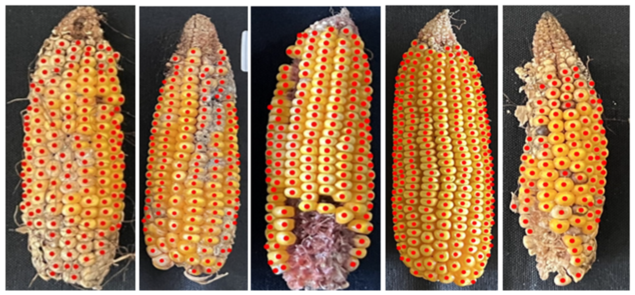
ANOVA for treatment effects on observed and predicted parameters was performed to evaluate whether the models developed for yield, kernel count, and HI showed the same effects as observed values. Variability of corn ear shape and size, and kernel development due to treatment effects are shown in Figure A3. In 2023, irrigation rates did not significantly affect any of the parameters (p > 0.1) due to excessive rainfall. In contrast, nitrogen rates had a significant effect on corn grain yield, kernel count/ear, and HI (Table 5). Residual diagnostics confirmed that the ANOVA assumptions were met. Post hoc analysis comparing the mean values of each nitrogen treatment is shown in Figure 10. Observed and predicted kernel count/ear (Figure 10a) and corn grain yield (Figure 10b) were significantly lower when plots did not receive any nitrogen application, with no significant differences observed among the nitrogen rates varying from 67 to 336 kg N ha−1. Predicted and observed HI (Figure 10c) increased when nitrogen rates of up to 135 kg N ha−1 were applied, after which a small decline occurred at higher rates. However, the predicted HI was slightly underestimated at 67, 135, and 336 kg N ha−1 nitrogen rates. Overall, the treatment effects in the observed datasets were also reflected in the predicted datasets, indicating that the model was able to capture treatment-related variability reliably. The 2024 dataset, which was used for model training, included effects of both irrigation and nitrogen treatments. However, because the data were divided into training and testing subsets, the complete treatment effects were not explicitly analyzed.
Table 5.
Analysis of Variance (Type III) for observed and model-predicted kernel count per ear, yield, and harvest index (HI), in response to nitrogen and irrigation treatments. Significance levels: *** p < 0.001; ** p < 0.01; * p < 0.1.
Figure 10.
Observed and model-predicted (a) kernel number per ear, (b) corn grain yield, and (c) harvest index (HI) across nitrogen rates. Capital letters denote significant differences among treatments for observed values, while lowercase letters denote significant differences for predicted values (α = 0.05).
4. Discussion
This study evaluated the effectiveness of deep learning detection models, their training strategies, and applicability in real-world agronomic scenarios for corn kernel detection and counting. Results demonstrated that the YOLO-based architecture, particularly when trained with transfer learning, provided a fast, accurate, and robust solution to count harvested corn ears for corn grain yield and yield parameters estimation.
4.1. The Efficacy of Transfer Learning and Architectural Choice in YOLO Models
A major finding was the consistent advantage of the fine-tuning model over the models trained from scratch. Across all YOLO versions, fine-tuned models started with lower initial loss values and converged more rapidly than their counterparts trained from scratch. These outcomes align with established literature showing that transfer learning accelerates convergence and improves generalization by leveraging features learned from large, diverse datasets such as COCO [74,75]. Although mild overfitting was observed in some fine-tuned models during training, their superior performance on the test set (e.g., YOLOv11x with fine-tuned training strategy achieving R2pred = 0.858 compared with R2pred = 0.841 for YOLOv11x with from-scratch training strategy) confirmed transfer learning as the optimal strategy for kernel detection and counting. Similar findings were reported for other applications. Zhou et al. [76] found that fine-tuned source-domain models outperformed those trained independently from scratch for soil moisture prediction. In addition, a study conducted in the medical field for tumor detection reported that although overall accuracy was comparable between fine-tuned and from scratch models, the fine-tuned model performed significantly better in clinically crucial aspects, such as reducing false alarms while maintaining true-positive (tumor) detection rates [77]. When comparing model architecture, most models demonstrate smooth and stable convergence. In contrast, YOLOv10x showed higher initial loss and less stable convergence, likely due to its NMS-free detection design, which introduces additional optimization complexity during training [61]. Another critical observation was the markedly higher latency of certain from-scratch models, particularly YOLOv9e (35.9 ms total latency) and YOLOv12x (27.1 ms), caused by excessive post-processing during NMS. Similar results were reported by Tian et al. [39], who observed a latency of 11.79 ms for YOLOv12x, which was higher than that of YOLOv10x (10.70 ms) and YOLOv11x (11.3 ms). The authors attributed this slower performance to two factors, (1) the quadratic computational complexity and (2) the inefficient memory access, which limited inference speed. Such high latency made these models unsuitable for real-time applications.
Among the evaluated architectures, YOLOv11x with the fine-tuned strategy achieved the best balance of accuracy and efficiency, with the lowest prediction error (MAE = 22.317, R2pred = 0.858) and one of the fastest inference speeds (4.8 ms). YOLOv8x and YOLOv5x also performed competitively, suggesting that older architecture remains effective for small-object detection tasks such as corn kernels. In contrast, YOLOv10x consistently underperformed, reflecting the difficulty of this architecture in detecting compact and densely arranged small objects. This is likely due to the NMS-free training and inference pipeline, which means that the model provides the one best output per object [61]. While this design improves efficiency and speed, it can reduce recall in dense small-object scenarios where overlapping bounding boxes are common. This accuracy and efficiency trade-off reflects a broader trend in YOLO evolution, where newer versions incorporate increasingly complex backbones and feature-fusion modules that do not always improve performance for tasks dominated by small objects [78]. By contrast, YOLOv11 was developed with architectural enhancements targeting small and occluded object detection, whereas YOLOv8 was refined to better detect objects of varying sizes and shapes within a single frame [62,78]. These design differences explain why YOLOv8x and YOLOv11x achieved superior performance, while YOLOv10x lagged in detecting tightly packed kernels. Similar results have been reported in other studies. For example, an evaluation of YOLOv5 through YOLOv11 for small-object detection (objects occupying 1%, 2.5%, and 5% of the image area) found that YOLOv8 achieved the best overall performance, followed by YOLOv11 [79]. Likewise, another study comparing YOLOv8 to YOLOv11 for weed detection reported that YOLOv11 achieved the fastest inference speed, followed by YOLOv8, consistent with our findings. However, in terms of accuracy, YOLOv9 had the best performance, with an mAP@0.5 of 0.935 [80]. Previous studies using YOLOv5 reported a precision of 96.1% for detecting broken and mildewed kernels in shelled samples [33], which provides a separation between kernels. In the current study, YOLOv5 achieved an even higher precision (97.9%) when detecting densely arranged kernels under optimized training strategies. Building on these findings, the systematic comparison in this study further demonstrates that for densely arranged kernel detection, newer architectures do not necessarily yield better performance, as YOLOv11x and YOLOv8x outperformed the more recent YOLOv12x, providing clearer guidance for model selection in small-object detection tasks.
4.2. Baseline Comparison with Faster R-CNN
YOLO significantly outperformed Faster R-CNN across all performance metrics. While Faster R-CNN achieved high precision (0.970), its recall was substantially lower (0.779), leading to higher undercounting errors (MAE = 59.294, R2pred = 0.116). Moreover, Faster R-CNN required longer training and inference times (9.2 h, 11 ms per image) compared with YOLO (1–1.3 h, <5 ms). These results are consistent with the known limitations of two-stage detectors in handling small, dense objects, where region proposal mechanisms often fail to capture every instance [60]. In contrast, YOLO’s single-stage design optimizes detection globally, allowing it to excel in tasks involving numerous, closely spaced objects such as corn kernels [78,81]. A study aligned with our findings reported that YOLO models demonstrated greater potential for detecting weed species both more accurately and quicker than Faster R-CNN [80]. Although later YOLO versions (v5–v12) have significantly improved, an earlier study presented differing conclusions. A study comparing YOLO v1–v4 and R-CNN showed that the FastR-CNN outperformed YOLO in detection accuracy (70.0 vs. 63.4). However, when comparing inference speed, YOLO was still approximately 300 times faster [82]. To have a comprehensive comparison and benchmarking, in the future, other state-of-the-art architectures, such as DETR [83] or EfficientDet [84] may provide additional insights into performance trade-offs.
4.3. Model Generalization and Agronomic Application
Another strength of this study was the demonstration of cross-year robustness. Models trained on 2024 datasets performed strongly on independent 2023 datasets, achieving a low MAPE of 2%. This result confirmed the ability of YOLOv8x and YOLOv11x to generalize across growing seasons with distinct environmental conditions. The growing season of 2023 was characterized by adequate rainfall, whereas 2024 experienced drought stress, as shown in Table 1. Therefore, the lower MAPE in 2023 compared to the 2024 test set (~10%) was likely due to more uniform ear development and healthy kernel under favorable moisture conditions, which reduced kernel occlusion and improved kernel detection accuracy. Cross-year validation is a critical step in developing phenotyping tools, ensuring that models are not overfitted to a single year or site [85]. The YOLO model tested in this study maintained high accuracy across contrasting growing seasons.
Predicted yield and HI from the YOLOv11x kernel count model showed strong agreement with observed yield (R2 = 0.881) and HI (R2 = 0.758). Yield is a complex trait determined not only by kernel number, but also by kernel weight, size, and moisture content [86]. Similarly, HI depends on multiple physiological factors. HI was calculated as grain yield divided by total AGB. Small errors between predicted and manually measured yield were reflected in the HI calculations and potentially worsened due to the ratio of yield and biomass, resulting in larger discrepancies for HI compared to yield prediction. However, the strong associations observed indicate that the model effectively captured key components contributing to yield formation. Moreover, the model also captured treatment-driven responses. The predicted models showed great performance in estimating yield and HI under varying nitrogen rates, clearly separating the zero-nitrogen treatment from fertilized treatments and reproducing the plateau response observed at higher nitrogen rates in manually counted kernels and observed yield. These results confirm that the models generalized effectively across years and experimental conditions of different nitrogen rates. Other studies have predicted corn yield using UAV canopy imagery and machine learning models, reporting R2 values ranging from 0.67 for individual models to 0.90 for ensemble approaches, often relying on large numbers of predictors derived from vegetation indices and spectral bands [87]. Other approaches using multimodal UAV-based multispectral, LiDAR, and meteorological data achieved R2 values around 0.78 [88]. Compared with these methods [87,89], the mobile phone image-based YOLO framework used in this study achieved comparable prediction accuracy (R2 = 0.881) while requiring fewer inputs and no specialized sensors, offering a simpler and low-cost alternative for yield estimation. Unlike the aforementioned methods that depend on multiple input parameters, this approach directly leverages kernel number, combined with test weight and plant population readily available to farmers and researchers, to provide a simplified and practical framework for yield prediction.
Despite the promising performance of the proposed framework, several limitations should be acknowledged. The dataset used in this study was collected during two growing seasons, but using only one genotype. The methods used in this study focused on field corn and favored a simpler and faster image acquisition process for indoor conditions, following standard agronomic practices. Model generalization and application for field conditions with varied backgrounds, and other corn types may be limited. Following the simple approach based on standard agronomic practices, kernel number was estimated from half-surface images and extrapolated to the whole ear by multiplication. However, in practical conditions, ears may not be uniform due to diseases, insect damage, or deformation, and kernel morphology varies across corn types such as dent and flint corn, which may introduce additional challenges and reduce prediction accuracy. Future research will be focused on developing decision-support tools or smart applications that incorporate more diverse genotypes, stress conditions, and field-acquired images in the training dataset to further improve model robustness and practical applicability. Nevertheless, this study advances existing research by systematically comparing two training strategies across six YOLO generations, demonstrating cross-year generalization, and linking kernel detection directly to agronomic traits such as yield and HI.
5. Conclusions
This research validates the application of state-of-the-art YOLO models as a powerful and efficient approach for automated corn kernel counting compared to Faster R-CNN. Results showed that transfer learning (fine-tuned model) significantly improved model performance, enabling faster convergence, higher prediction accuracy, and lower inference latency compared with models trained from scratch. Among the tested YOLO architectures, YOLOv11x exhibited the highest predictive accuracy, achieving an R2pred of 0.858 for both test and 0.890 for cross-year images, indicating strong generalization across different datasets. In addition to accurate kernel detection, the model successfully estimated predicted yield and the yield component HI, with R2 values of 0.881 and 0.758, respectively, under different management practices, demonstrating its potential for agronomic applications. Overall, these findings highlight the potential of smartphone image-based models as reliable tools for phenotyping and data-driven yield prediction in corn production systems.
Future work will be focused on improving the robustness and practical deployment of the proposed framework. An interactive web-based application will be developed to allow users to upload corn ear images from mobile devices, perform real-time kernel detection, and estimate yield using test-weight and seeding rates. In addition, future research will include multi-genotype and multi-environment validation and explore the integration of additional traits such as kernel size and ear morphology to further improve estimation accuracy.
Author Contributions
B.G.: Conceptualization, Data curation, Formal analysis, Investigation, Methodology, Software, Validation, Visualization, Writing—original draft, Writing—review and editing; L.N.L.: Conceptualization, Funding Acquisition, Investigation, Methodology, Project administration, Supervision, Validation, Visualization, Resources, Writing—original draft, Writing—review and editing; T.B.: Conceptualization, Validation, Writing—review and editing; G.L.: Conceptualization, Validation, Writing—review and editing. All authors have read and agreed to the published version of the manuscript.
Funding
This research received no external funding.
Institutional Review Board Statement
Not applicable.
Informed Consent Statement
Not applicable.
Data Availability Statement
Data will be made available on request.
Acknowledgments
The authors thank the members of the Lacerda Lab for their assistance with field experiment setup and data collection. We also acknowledge the J. Phil Campbell Research and Education Center Iron Horse Plant Sciences Farm team for their support and provision of resources essential to completing the field research.
Conflicts of Interest
The authors declare that they have no known competing financial interests or personal relationships that could have appeared to influence the work reported in this paper.
Abbreviations
The following abbreviations are used in this manuscript:
| YOLO | You Only Look Once |
| R-CNN | Region-based Convolutional Neural Network |
| CK-CNN | Custom Kernel Convolutional Neural Network |
| VGG-16 | Visual Geometry Group 16-Layer Network |
| ResNet50 | Residual Network with 50 Layers |
| NMS | Non-Maximum Suppression |
| UAN | Urea Ammonium Nitrate |
| MAE | Mean Absolute Error |
| MaxAE | Maximum Absolute Error |
| RMSE | Root Mean Square Error |
| MAPE | Mean Absolute Percentage Error |
| R2 | Coefficient of Determination (R-squared) |
| R2pred | Prediction Accuracy (R-squared) |
| TP | True Positive |
| FP | False Positive |
| FN | False Negative |
| mAP@0.5 | Mean Average Precision at an Intersection over Union (IoU) threshold of 0.5 |
| mAP@0.5:0.95 | Mean Average Precision averaged across multiple IoU thresholds from 0.5 to 0.95 in increments of 0.05 |
| IoU | Intersection over Union |
| ms | Milliseconds |
| FPN | Feature Pyramid Network |
| 1000-GW | Thousand Grain Weight |
Appendix A
Figure A1.
Visualization of kernel detection results from different models (Faster R-CNN, YOLOv11, and YOLOv8). Red dots represent the detected kernel centers used for kernel counting.
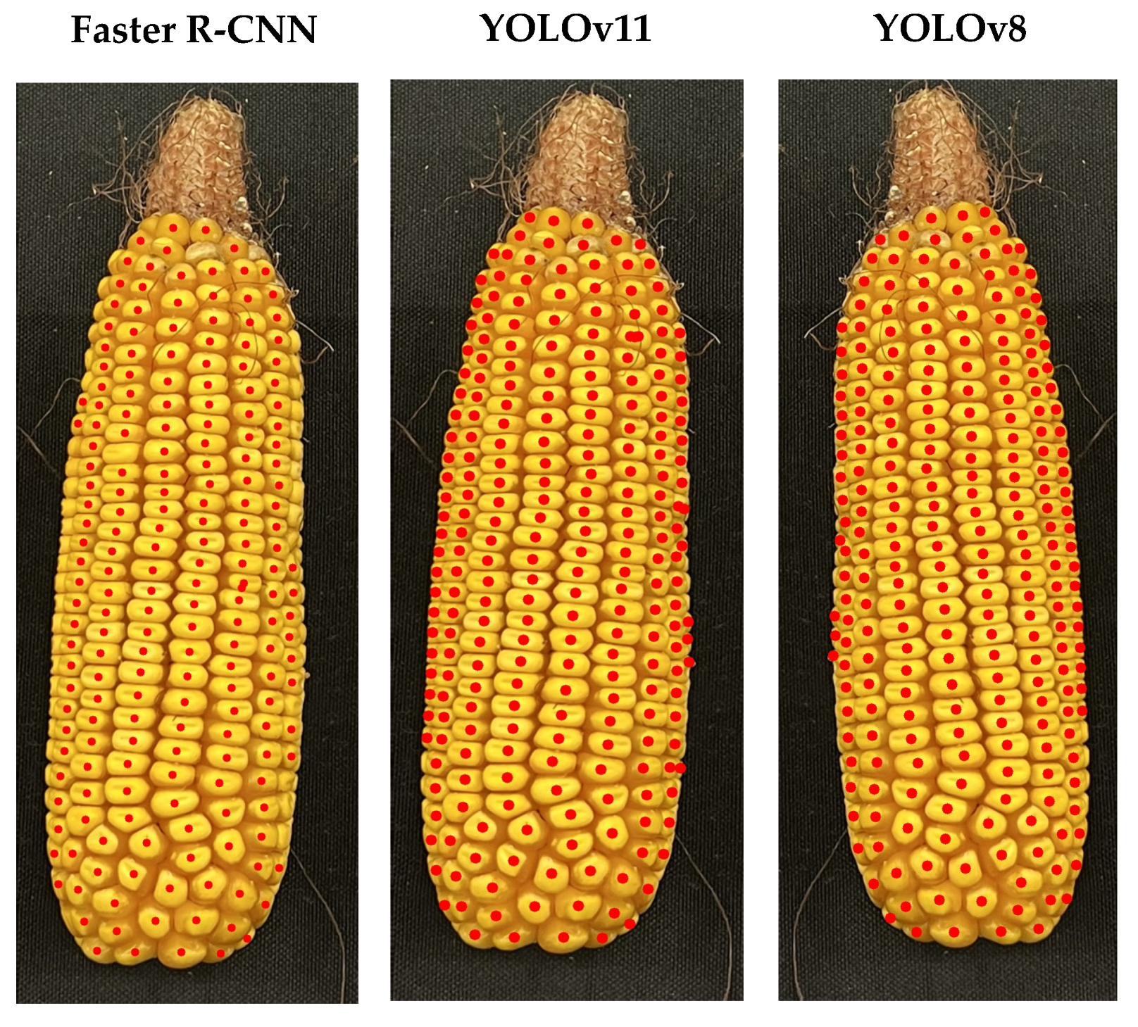
Figure A2.
Examples of the best- and worst-performing predictions from the YOLOv11x model for kernel detection. (a) Ears with minimal prediction error (%Err = 0.09–0.1), representing highly accurate kernel detection. (b) Cases with higher errors (%Err = 10–13) due to irregular kernel alignment and occlusion. Blue dots indicate kernels predicted by the model, and red dots indicate missing kernels.
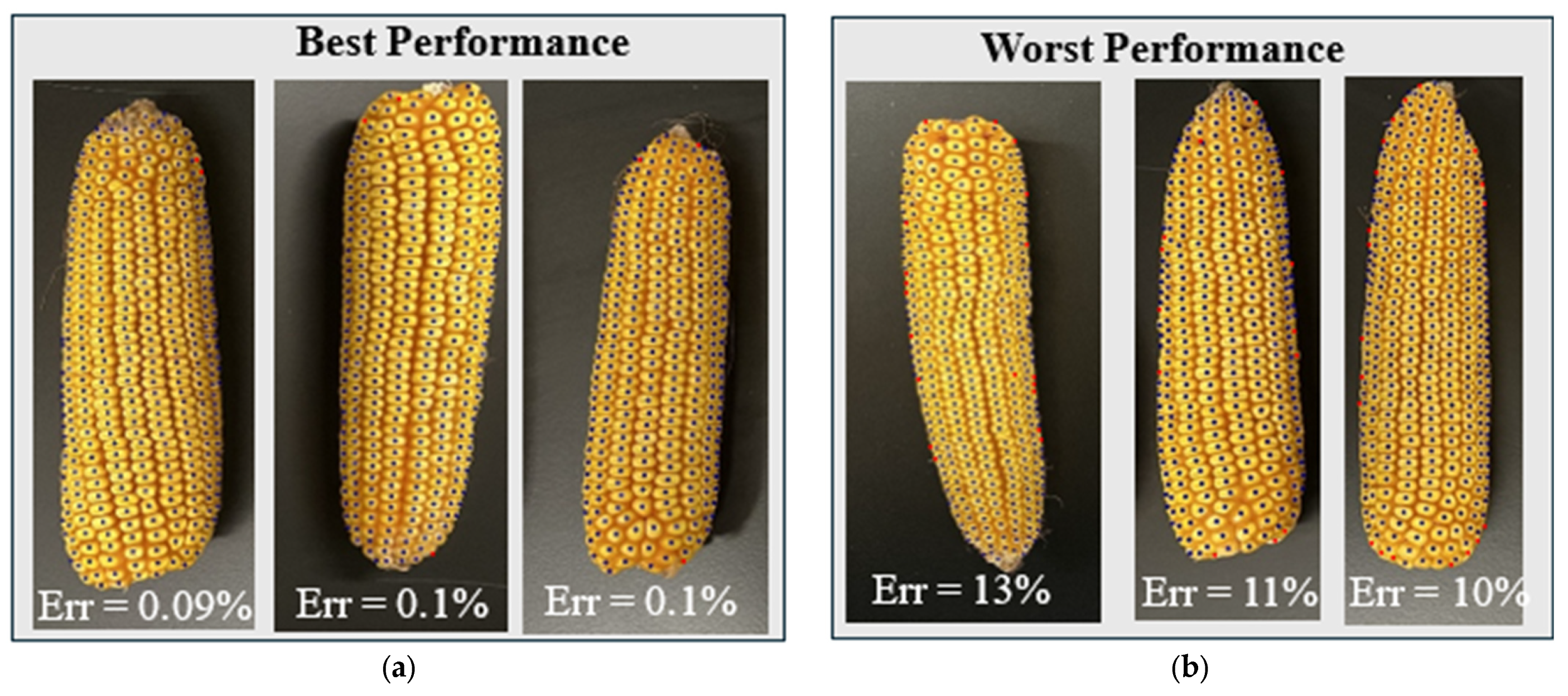
Figure A3.
Examples illustrate the high variability in corn ear shape, size, and kernel development resulting from different treatments, along with the application of the YOLOv11x model. Each red dot represents an individual kernel detected by the model.
References
- Erenstein, O.; Jaleta, M.; Sonder, K.; Mottaleb, K.; Prasanna, B.M. Global Maize Production, Consumption and Trade: Trends and R&D Implications. Food Sec. 2022, 14, 1295–1319. [Google Scholar] [CrossRef] [Scilit]
- Loy, D.D.; Lundy, E.L. Nutritional Properties and Feeding Value of Corn and Its Coproducts. In Corn, 3rd ed.; Serna-Saldivar, S.O., Ed.; AACC International Press: Oxford, UK, 2019; pp. 633–659. ISBN 978-0-12-811971-6. [Google Scholar]
- Gilbert, C.L.; Mugera, H.K. Competitive Storage, Biofuels and the Corn Price. J. Agric. Econ. 2020, 71, 384–411. [Google Scholar] [CrossRef] [Scilit]
- USDA. USDA ERS—Feed Grains Sector at a Glance. Available online: https://www.ers.usda.gov/topics/crops/corn-and-other-feed-grains/feed-grains-sector-at-a-glance/ (accessed on 5 February 2024).
- Fischer, R.A.; Byerlee, D.; Edmeades, G.O. (PDF) Crop Yields and Global Food Security: Will Yield Increase Continue to Feed the World? ACIAR Monograph No. 158. Australian Centre for International Agricultural Research. Available online: https://www.researchgate.net/publication/282713287_Crop_yields_and_global_food_security_will_yield_increase_continue_to_feed_the_world_ACIAR_Monograph_No_158_Australian_Centre_for_International_Agricultural_Research (accessed on 4 March 2024).
- Prasanna, B.M.; Cairns, J.E.; Zaidi, P.H.; Beyene, Y.; Makumbi, D.; Gowda, M.; Magorokosho, C.; Zaman-Allah, M.; Olsen, M.; Das, A.; et al. Beat the Stress: Breeding for Climate Resilience in Maize for the Tropical Rainfed Environments. Theor. Appl. Genet. 2021, 134, 1729–1752. [Google Scholar] [CrossRef] [Scilit] [PubMed]
- Amini, R. Assessment of Yield and Yield Components of Corn (Zea mays L.) under Two Three Strip Intercropping Systems. Int. J. Biosci. (IJB) 2013, 3, 65–69. [Google Scholar] [CrossRef] [Scilit]
- Cambouris, A.; Ziadi, N.; Perron, I.; Alotaibi, K.; St. Luce, M.; Tremblay, N. Corn Yield Components Response to Nitrogen Fertilizer as a Function of Soil Texture. Can. J. Soil. Sci. 2016, 96, 386–399. [Google Scholar] [CrossRef] [Scilit]
- Khalafi, A.; Mohsenifar, K.; Gholami, A.; Barzegari, M. Corn (Zea mays L.) Growth, Yield and Nutritional Properties Affected by Fertilization Methods and Micronutrient Use. Int. J. Plant Prod. 2021, 15, 589–597. [Google Scholar] [CrossRef] [Scilit]
- Veenstra, R.L.; Messina, C.D.; Berning, D.; Haag, L.A.; Carter, P.; Hefley, T.J.; Prasad, P.V.V.; Ciampitti, I.A. Corn Yield Components Can Be Stabilized via Tillering in Sub-Optimal Plant Densities. Front. Plant Sci. 2023, 13, 1047268. [Google Scholar] [CrossRef] [Scilit]
- Fernández, J.A.; Messina, C.D.; Salinas, A.; Prasad, P.V.V.; Nippert, J.B.; Ciampitti, I.A. Kernel Weight Contribution to Yield Genetic Gain of Maize: A Global Review and US Case Studies. J. Exp. Bot. 2022, 73, 3597–3609. [Google Scholar] [CrossRef] [Scilit]
- Gheith, E.M.S.; El-Badry, O.Z.; Lamlom, S.F.; Ali, H.M.; Siddiqui, M.H.; Ghareeb, R.Y.; El-Sheikh, M.H.; Jebril, J.; Abdelsalam, N.R.; Kandil, E.E. Maize (Zea mays L.) Productivity and Nitrogen Use Efficiency in Response to Nitrogen Application Levels and Time. Front. Plant Sci. 2022, 13, 941343. [Google Scholar] [CrossRef] [Scilit]
- Li, Y.; Guan, K.; Peng, B.; Franz, T.E.; Wardlow, B.; Pan, M. Quantifying Irrigation Cooling Benefits to Maize Yield in the US Midwest. Glob. Change Biol. 2020, 26, 3065–3078. [Google Scholar] [CrossRef] [Scilit]
- Rizzo, G.; Monzon, J.P.; Tenorio, F.A.; Howard, R.; Cassman, K.G.; Grassini, P. Climate and Agronomy, Not Genetics, Underpin Recent Maize Yield Gains in Favorable Environments. Proc. Natl. Acad. Sci. USA 2022, 119, e2113629119. [Google Scholar] [CrossRef] [Scilit] [PubMed]
- Subedi, K.D.; Ma, B.L. Corn Crop Production Growth, Fertilization and Yield; Nova Science Publishers: Hauppauge, NY, USA, 2011. [Google Scholar] [CrossRef]
- Wu, D.; Cai, Z.; Han, J.; Qin, H. Automatic Kernel Counting on Maize Ear Using RGB Images. Plant Methods 2020, 16, 79. [Google Scholar] [CrossRef] [Scilit] [PubMed]
- Dunđerski, D.; Jaćimović, G.; Crnobarac, J.; Visković, J.; Latković, D. Using Digital Image Analysis to Estimate Corn Ear Traits in Agrotechnical Field Trials: The Case with Harvest Residues and Fertilization Regimes. Agriculture 2023, 13, 732. [Google Scholar] [CrossRef] [Scilit]
- Matias, F.I.; Caraza-Harter, M.V.; Endelman, J.B. FIELDimageR: An R Package to Analyze Orthomosaic Images from Agricultural Field Trials. Plant Phenome J. 2020, 3, e20005. [Google Scholar] [CrossRef] [Scilit]
- Liang, X.; Ye, J.; Li, X.; Tang, Z.; Zhang, X.; Li, W.; Yan, J.; Yang, W. A High-Throughput and Low-Cost Maize Ear Traits Scorer. Mol. Breed. 2021, 41, 17. [Google Scholar] [CrossRef] [Scilit]
- dos Santos de Arruda, M.; Osco, L.; Acosta, P.; Gonçalves, D.; Junior, J.; Ramos, A.P.; Matsubara, E.; Luo, Z.; Li, J.; Silva, J.; et al. Counting and Locating High-Density Objects Using Convolutional Neural Network. Expert Syst. Appl. 2022, 195, 116555. [Google Scholar] [CrossRef] [Scilit]
- Kılıç, E.; Ozturk, S. An Accurate Car Counting in Aerial Images Based on Convolutional Neural Networks. J. Ambient Intell. Humaniz. Comput. 2021, 14, 1259–1268. [Google Scholar] [CrossRef] [Scilit]
- Krizhevsky, A.; Sutskever, I.; Hinton, G.E. ImageNet Classification with Deep Convolutional Neural Networks. In Proceedings of the Advances in Neural Information Processing Systems; Curran Associates, Inc.: New York, NY, USA, 2012; Volume 25. [Google Scholar]
- Rani, S.; Ghai, D.; Kumar, S.; Kantipudi, M.P.; Alharbi, A.H.; Ullah, M.A. Efficient 3D AlexNet Architecture for Object Recognition Using Syntactic Patterns from Medical Images. Comput. Intell. Neurosci. 2022, 2022, 7882924. [Google Scholar] [CrossRef] [Scilit]
- Akbarpour, O.; Akbari, S.; Fanourakis, D.; Taheri-Garavand, A. Deep learning-based seed variety classification: A case study in maize. BMC Plant Biology 2026, 26, 105. [Google Scholar] [CrossRef] [Scilit]
- Velesaca, H.; Mira, R.; Suarez, P.; Larrea, C.; Sappa, A. Deep Learning Based Corn Kernel Classification. In IEEE/CVF Conference on Computer Vision and Pattern Recognition (CVPR) Workshops, Seattle, WA, USA, 14–19 June 2020; IEEE: New York, NY, USA, 2020; p. 302. [Google Scholar]
- He, K.; Gkioxari, G.; Dollár, P.; Girshick, R. Mask R-CNN. In 2017 IEEE International Conference on Computer Vision (ICCV), Venice, Italy, 22–29 October 2017; IEEE: New York, NY, USA, 2017; pp. 2980–2988. [Google Scholar]
- Simonyan, K.; Zisserman, A. Very Deep Convolutional Networks for Large-Scale Image Recognition. arXiv 2014. [Google Scholar] [CrossRef] [Scilit]
- He, K.; Zhang, X.; Ren, S.; Sun, J. Deep Residual Learning for Image Recognition. In 2016 IEEE Conference on Computer Vision and Pattern Recognition (CVPR), Las Vegas, NV, USA, 27–30 June 2016; IEEE: New York, NY, USA, 2016; pp. 770–778. [Google Scholar]
- Wang, L.; Liu, J.; Zhang, J.; Wang, J.; Fan, X. Corn Seed Defect Detection Based on Watershed Algorithm and Two-Pathway Convolutional Neural Networks. Front. Plant Sci. 2022, 13, 730190. [Google Scholar] [CrossRef] [Scilit] [PubMed]
- Khaki, S.; Pham, H.; Han, Y.; Kuhl, A.; Kent, W.; Wang, L. Convolutional Neural Networks for Image-Based Corn Kernel Detection and Counting. Sensors 2020, 20, 2721. [Google Scholar] [CrossRef] [Scilit] [PubMed]
- Khaki, S.; Pham, H.; Han, Y.; Kuhl, A.; Kent, W.; Wang, L. DeepCorn: A Semi-Supervised Deep Learning Method for High-Throughput Image-Based Corn Kernel Counting and Yield Estimation. Knowl.-Based Syst. 2021, 218, 106874. [Google Scholar] [CrossRef] [Scilit]
- Murat, A.A.; Kiran, M.S. A Comprehensive Review on YOLO Versions for Object Detection. Eng. Sci. Technol. Int. J. 2025, 70, 102161. [Google Scholar] [CrossRef] [Scilit]
- Liu, M.; Liu, Y.; Wang, Q.; He, Q.; Geng, D. Real-Time Detection Technology of Corn Kernel Breakage and Mildew Based on Improved YOLOv5s. Agriculture 2024, 14, 725. [Google Scholar] [CrossRef] [Scilit]
- Wang, Q.; Yang, H.; He, Q.; Yue, D.; Zhang, C.; Geng, D. Real-Time Detection System of Broken Corn Kernels Based on BCK-YOLOv7. Agronomy 2023, 13, 1750. [Google Scholar] [CrossRef] [Scilit]
- Li, W.; Zhang, Y. DC-YOLO: An Improved Field Plant Detection Algorithm Based on YOLOv7-Tiny. Sci. Rep. 2024, 14, 26430. [Google Scholar] [CrossRef] [Scilit]
- Hobbs, J.; Khachatryan, V.; Anandan, B.S.; Hovhannisyan, H.; Wilson, D. Broad Dataset and Methods for Counting and Localization of On-Ear Corn Kernels. Front. Robot. AI 2021, 8, 627009. [Google Scholar] [CrossRef] [Scilit]
- Jochers, G.; Stoken, J.; Chaurasia, A.; Hajek, J.; Kwon, C.; Tao, A.; Kwon, Y.; Wang, T.; Fang, L. Home. Available online: https://github.com/ultralytics/yolov5 (accessed on 26 June 2025).
- Jocher, G.; Qiu, J.; Chaurasia, A. Ultralytics YOLO. 2023. Available online: https://github.com/ultralytics/ultralytics (accessed on 26 June 2025).
- Tian, Y.; Ye, Q.; Doermann, D. YOLOv12: Attention-Centric Real-Time Object Detectors. arXiv 2025, arXiv:2502.12524. [Google Scholar]
- Zoph, B.; Ghiasi, G.; Lin, T.-Y.; Cui, Y.; Liu, H.; Cubuk, E.D.; Le, Q.V. Rethinking Pre-Training and Self-Training. In Proceedings of the Advances in Neural Information Processing Systems 33 (NeurIPS 2020), Virtual, 6–12 December 2020. [Google Scholar]
- Shen, Z.; Liu, Z.; Li, J.; Jiang, Y.-G.; Chen, Y.; Xue, X. DSOD: Learning Deeply Supervised Object Detectors from Scratch. In 2017 IEEE International Conference on Computer Vision, Venice, Italy, 22–29 October 2017; IEEE: New York, NY, USA, 2018. [Google Scholar]
- Ray, I.; Raipuria, G.; Singhal, N. Rethinking ImageNet Pre-Training for Computational Histopathology. In 2022 44th Annual International Conference of the IEEE Engineering in Medicine & Biology Society (EMBC), Glasgow, UK, 11–15 July 2022; IEEE: New York, NY, USA, 2022; pp. 3059–3062. [Google Scholar]
- Wen, Y.; Chen, L.; Deng, Y.; Zhou, C. Rethinking Pre-Training on Medical Imaging. J. Vis. Commun. Image Represent. 2021, 78, 103145. [Google Scholar] [CrossRef] [Scilit]
- Ferreira, C.S.S.; Pires, A.F.; Pereira, A.; Mendes-Moreira, P.; Harrison, M.T. Modest Irrigation Frequency Improves Maize Water Use Efficiency and Influences Trait Expression. Sustainability 2025, 17, 7365. [Google Scholar] [CrossRef] [Scilit]
- Wang, B.; Liu, C.; Zhang, D.; He, C.; Zhang, J.; Li, Z. Effects of Maize Organ-Specific Drought Stress Response on Yields from Transcriptome Analysis. BMC Plant Biol. 2019, 19, 335. [Google Scholar] [CrossRef] [Scilit]
- Szulc, P.; Nowosad, K.; Bocianowski, J. Morphological Traits in Maize Cultivars at Varied N and Mg Fertilization Rates. Pol. J. Agron. 2016, 25, 35–40. [Google Scholar]
- Hammad, H.M.; Abbas, F.; Ahmad, A.; Bakhat, H.F.; Farhad, W.; Wilkerson, C.J.; Fahad, S.; Hoogenboom, G. Predicting Kernel Growth of Maize under Controlled Water and Nitrogen Applications. Int. J. Plant Prod. 2020, 14, 609–620. [Google Scholar] [CrossRef] [Scilit]
- Nielsen, B. Effects of Severe Stress During Grain Filling in Corn. Pest&Crop Newsletter. 2018. Issue 2018.17. Available online: https://extension.entm.purdue.edu/newsletters/pestandcrop/article/effects-of-severe-stress-during-grain-filling-in-corn/ (accessed on 12 March 2026).
- DKC68-48 BRAND NATIONAL|Crop Science US. Available online: https://www.cropscience.bayer.us/d/dekalb-dkc68-48-corn (accessed on 18 August 2025).
- Migliaccio, K.W.; Morgan, K.T.; Vellidis, G.; Zotarelli, L.; Fraisse, C.; Rowland, D.L.; Andreis, J.H.; Crane, J.H.; Zurweller, B.A. Smartphone Apps for Irrigation Scheduling; American Society of Agricultural and Biological Engineers: St. Joseph, MI, USA, 2015; pp. 1–16. [Google Scholar]
- Ngoune Tandzi, L.; Mutengwa, C.S. Estimation of Maize (Zea mays L.) Yield Per Harvest Area: Appropriate Methods. Agronomy 2020, 10, 29. [Google Scholar] [CrossRef] [Scilit]
- Nielsen, R.L. Estimating Corn Grain Yield Prior to Harvest. Purdue University. Available online: https://www.agry.purdue.edu/ext/corn/news/timeless/YldEstMethod.html (accessed on 3 January 2026).
- Donald, C.M.; Hamblin, J. The Biological Yield and Harvest Index of Cereals as Agronomic and Plant Breeding Criteria. In Advances in Agronomy; Brady, N.C., Ed.; Academic Press: Cambridge, MA, USA, 1976; Volume 28, pp. 361–405. [Google Scholar]
- DeLougherty, R.L.; Crookston, R.K. Harvest Index of Corn Affected by Population Density, Maturity Rating, and Environment. Agron. J. 1979, 71, 577–580. [Google Scholar] [CrossRef] [Scilit]
- Bennetzen, J.; Hake, S. Handbook of Maize: Its Biology; Springer: New York, NY, USA, 2009; ISBN 978-0-387-79417-4. [Google Scholar]
- Bonnett, O.T. The Inflorescences of Maize. Science 1954, 120, 77–87. [Google Scholar] [CrossRef] [Scilit]
- Araújo, F.; Gadelha, I.; Tsukahara, R.; Pita, L.; Costa, F.; Vaz, I.; Santos, A.; Fôlego, G. Hinting Pipeline and Multivariate Regression CNN for Maize Kernel Counting on the Ear. In 2023 IEEE International Conference on Image Processing (ICIP), Kuala Lumpur, Malaysia, 8–11 October 2023; IEEE: New York, NY, USA, 2023. [Google Scholar]
- Apeinans, I. Optimal Size of Agricultural Dataset for YOLOv8 Training. In Proceedings of the International Scientific and Practical Conference, Rezekne, Latvia, 27–28 June 2024; Volume 2. [Google Scholar]
- Roboflow: Computer Vision Tools for Developers and Enterprises. Available online: https://roboflow.com (accessed on 18 August 2025).
- Alhashmi, S.A.; Al-azawi, A. A Review of the Single-Stage vs. Two-Stage Detectors Algorithm: Comprehensive Insights into Object Detection. Int. J. Environ. Sci. 2025, 11, 775–787. [Google Scholar]
- Wang, A.; Chen, H.; Liu, L.; Chen, K.; Lin, Z.; Han, J.; Ding, G. YOLOv10: Real-Time End-to-End Object Detection. In Proceedings of the Advances in Neural Information Processing Systems 37 (NeurIPS 2024), Vancouver, BC, Canada, 10–15 December 2024. [Google Scholar]
- Khanam, R.; Hussain, M. YOLOv11: An Overview of the Key Architectural Enhancements. arXiv 2024, arXiv:2410.17725. [Google Scholar] [CrossRef] [Scilit]
- Ren, S.; He, K.; Girshick, R.; Sun, J. Faster R-CNN: Towards Real-Time Object Detection with Region Proposal Networks. IEEE Trans. Pattern Anal. Mach. Intell. 2017, 39, 1137–1149. [Google Scholar] [CrossRef] [Scilit]
- Lin, T.-Y.; Dollár, P.; Girshick, R.; He, K.; Hariharan, B.; Belongie, S. Feature Pyramid Networks for Object Detection. In 2017 IEEE Conference on Computer Vision and Pattern Recognition (CVPR), Honolulu, HI, USA, 21–26 July 2017; IEEE: New York, NY, USA, 2017; pp. 936–944. [Google Scholar]
- Paszke, A.; Gross, S.; Massa, F.; Lerer, A.; Bradbury, J.; Chanan, G.; Killeen, T.; Lin, Z.; Gimelshein, N.; Antiga, L.; et al. PyTorch: An imperative style, high-performance deep learning library. In Proceedings of the Advances in Neural Information Processing Systems 32 (NeurIPS 2019); Vancouver, BC, Canada, 8–14 December 2019; pp. 8024–8035. Available online: https://proceedings.neurips.cc/paper_files/paper/2019/file/bdbca288fee7f92f2bfa9f7012727740-Paper.pdf (accessed on 2 February 2026).
- Culjak, I.; Abram, D.; Pribanic, T.; Dzapo, H.; Cifrek, M. A Brief Introduction to OpenCV. In Proceedings of the 2012 Proceedings of the 35th International Convention MIPRO, Opatija, Croatia, 21–25 May 2012; pp. 1725–1730. [Google Scholar]
- Harris, C.R.; Millman, K.J.; van der Walt, S.J.; Gommers, R.; Virtanen, P.; Cournapeau, D.; Wieser, E.; Taylor, J.; Berg, S.; Smith, N.J.; et al. Array Programming with NumPy. Nature 2020, 585, 357–362. [Google Scholar] [CrossRef] [Scilit] [PubMed]
- Pedregosa, F.; Varoquaux, G.; Gramfort, A.; Michel, V.; Thirion, B.; Grisel, O.; Blondel, M.; Prettenhofer, P.; Weiss, R.; Dubourg, V.; et al. Scikit-Learn: Machine Learning in Python. J. Mach. Learn. Res. 2011, 12, 2825–2830. [Google Scholar]
- The Pandas Development Team. Pandas-Dev/Pandas: Pandas. Zenodo 2026. [Google Scholar] [CrossRef] [Scilit]
- Hunter, J.D. Matplotlib: A 2D Graphics Environment. Comput. Sci. Eng. 2007, 9, 90–95. [Google Scholar] [CrossRef] [Scilit]
- Bates, D.; Mächler, M.; Bolker, B.; Walker, S. Fitting Linear Mixed-Effects Models Using Lme4. J. Stat. Softw. 2015, 67, 1–48. [Google Scholar] [CrossRef] [Scilit]
- Lenth, R.V.; Piaskowski, J.; Banfai, B.; Bolker, B.; Buerkner, P.; Giné-Vázquez, I.; Hervé, M.; Jung, M.; Love, J.; Miguez, F.; et al. Emmeans: Estimated Marginal Means, Aka Least-Squares Means; The R Foundation: Vienna, Austria, 2025. [Google Scholar]
- Graves, S.; Piepho, H.-P.; Selzer, L.; Dorai-Raj, S. multcompView: Visualizations of Paired Comparisons; The R Foundation: Vienna, Austria, 2026. [Google Scholar]
- Kamilaris, A.; Prenafeta-Boldú, F.X. Deep Learning in Agriculture: A Survey. Comput. Electron. Agric. 2018, 147, 70–90. [Google Scholar] [CrossRef] [Scilit]
- Tan, C.; Sun, F.; Kong, T.; Zhang, W.; Yang, C.; Liu, C. A Survey on Deep Transfer Learning. In Proceedings of the 27th International Conference on Artificial Neural Networks, Rhodes, Greece, 4–7 October 2018. [Google Scholar]
- Zhou, T.; Ma, S.; Liu, T.; Yao, S.; Li, S.; Gao, Y. Integrating UAV-Based Multispectral Data and Transfer Learning for Soil Moisture Prediction in the Black Soil Region of Northeast China. Agronomy 2025, 15, 759. [Google Scholar] [CrossRef] [Scilit]
- Hasei, J.; Nakahara, R.; Otsuka, Y.; Takeuchi, K.; Nakamura, Y.; Ikuta, K.; Osaki, S.; Tamiya, H.; Miwa, S.; Ohshika, S.; et al. Utility of Same-Modality, Cross-Domain Transfer Learning for Malignant Bone Tumor Detection on Radiographs: A Multi-Faceted Performance Comparison with a Scratch-Trained Model. Cancers 2025, 17, 3144. [Google Scholar] [CrossRef] [Scilit]
- Ali, M.L.; Zhang, Z. The YOLO Framework: A Comprehensive Review of Evolution, Applications, and Benchmarks in Object Detection. Computers 2024, 13, 336. [Google Scholar] [CrossRef] [Scilit]
- Tariq, M.F.; Javed, M.A. Small Object Detection with YOLO: A Performance Analysis Across Model Versions and Hardware. arXiv 2025, arXiv:2504.09900. [Google Scholar] [CrossRef] [Scilit]
- Sharma, A.; Kumar, V.; Longchamps, L. Comparative Performance of YOLOv8, YOLOv9, YOLOv10, YOLOv11 and Faster R-CNN Models for Detection of Multiple Weed Species. Smart Agric. Technol. 2024, 9, 100648. [Google Scholar] [CrossRef] [Scilit]
- Redmon, J.; Divvala, S.; Girshick, R.; Farhadi, A. You Only Look Once: Unified, Real-Time Object Detection. In Proceedings of the 2016 IEEE Conference on Computer Vision and Pattern Recognition (CVPR), Las Vegas, NV, USA, 27–30 June 2016; IEEE: New York, NY, USA, 2016; pp. 779–788. [Google Scholar]
- Diwan, T.; Anirudh, G.; Tembhurne, J.V. Object Detection Using YOLO: Challenges, Architectural Successors, Datasets and Applications. Multimed. Tools Appl. 2023, 82, 9243–9275. [Google Scholar] [CrossRef] [Scilit]
- Carion, N.; Massa, F.; Synnaeve, G.; Usunier, N.; Kirillov, A.; Zagoruyko, S. End-to-End Object Detection with Transformers. In Proceedings of the 16th European Conference, Glasgow, UK, 23–28 August 2020. [Google Scholar]
- Tan, M.; Pang, R.; Le, Q.V. EfficientDet: Scalable and Efficient Object Detection. In Proceedings of the 2020 IEEE/CVF Conference on Computer Vision and Pattern Recognition (CVPR), Seattle, WA, USA, 13–19 June 2020; IEEE: New York, NY, USA, 2020; pp. 10778–10787. [Google Scholar]
- Ghosal, S.; Blystone, D.; Singh, A.K.; Ganapathysubramanian, B.; Singh, A.; Sarkar, S. An Explainable Deep Machine Vision Framework for Plant Stress Phenotyping. Proc. Natl. Acad. Sci. USA 2018, 115, 4613–4618. [Google Scholar] [CrossRef] [Scilit]
- Olmedo Pico, L.B.; Vyn, T.J. Dry Matter Gains in Maize Kernels Are Dependent on Their Nitrogen Accumulation Rates and Duration during Grain Filling. Plants 2021, 10, 1222. [Google Scholar] [CrossRef] [Scilit]
- Kumar, C.; Dhillon, J.; Huang, Y.; Reddy, K. Explainable Machine Learning Models for Corn Yield Prediction Using UAV Multispectral Data. Comput. Electron. Agric. 2025, 231, 109990. [Google Scholar] [CrossRef] [Scilit]
- Zhou, W.; Song, C.; Liu, C.; Fu, Q.; An, T.; Wang, Y.; Sun, X.; Wen, N.; Tang, H.; Wang, Q. A Prediction Model of Maize Field Yield Based on the Fusion of Multitemporal and Multimodal UAV Data: A Case Study in Northeast China. Remote Sens. 2023, 15, 3483. [Google Scholar] [CrossRef] [Scilit]
- Zhou, Y.; Ma, S.; Zhang, H.; Aakur, S. Enhancing Corn Yield Prediction: Optimizing Data Quality or Model Complexity? Smart Agric. Technol. 2024, 9, 100671. [Google Scholar] [CrossRef] [Scilit]
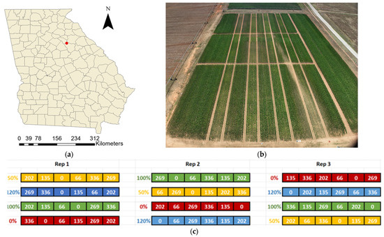
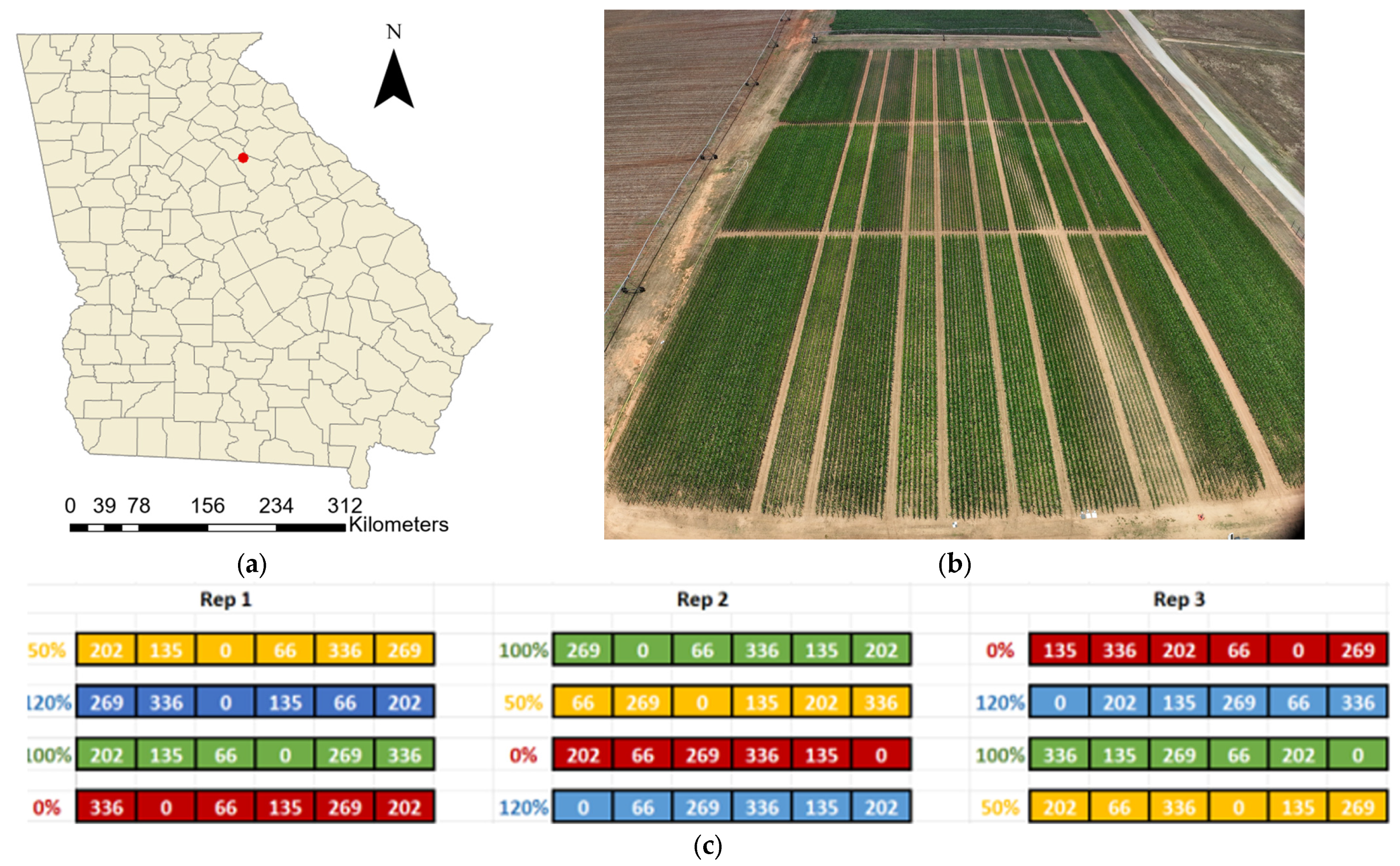
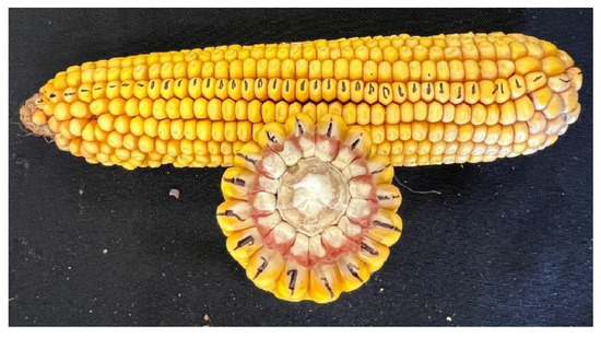
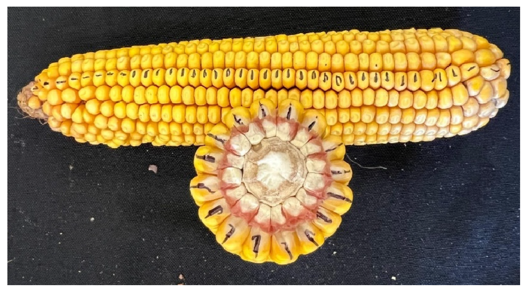
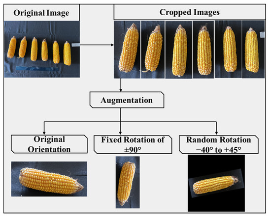
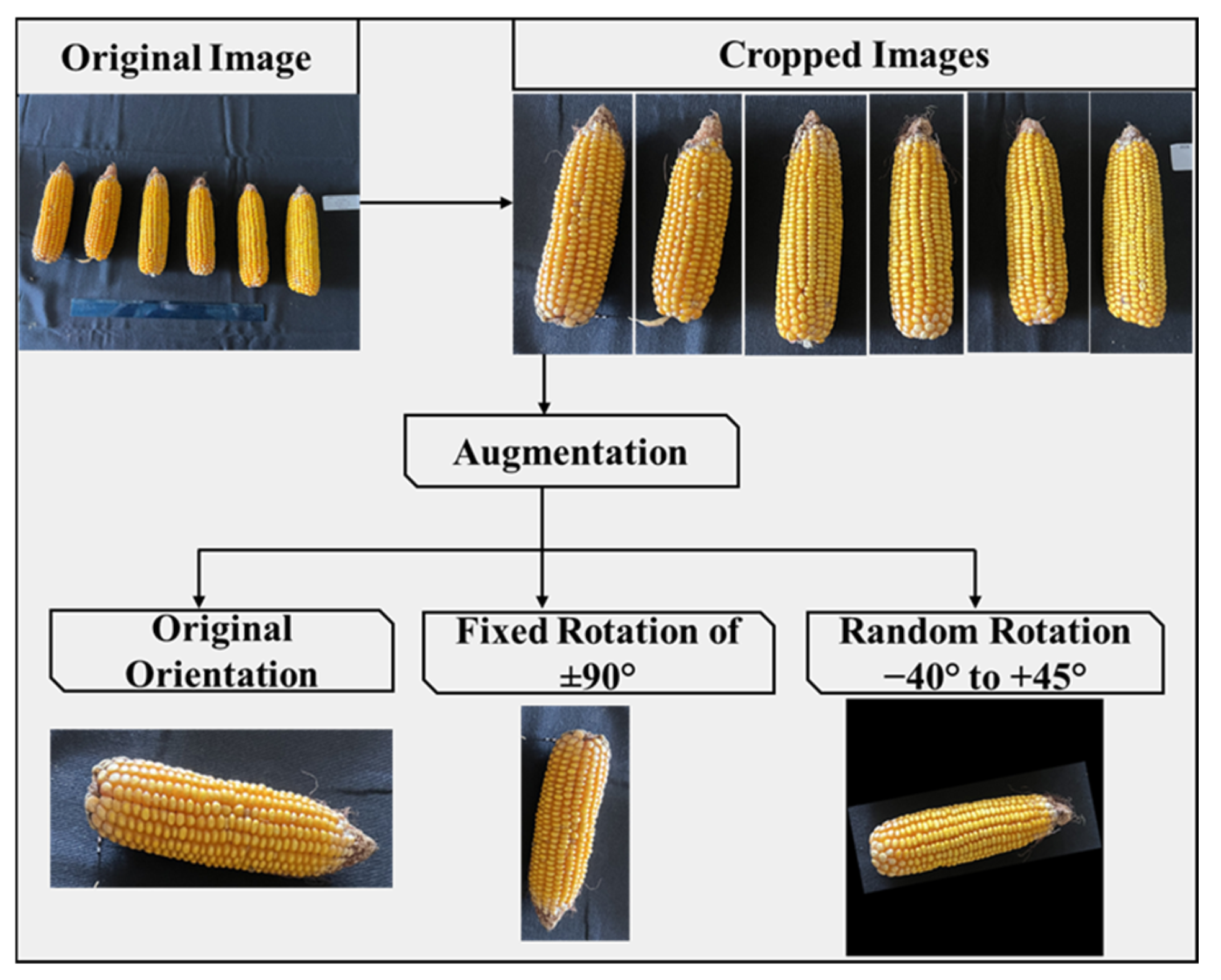
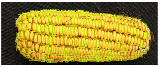
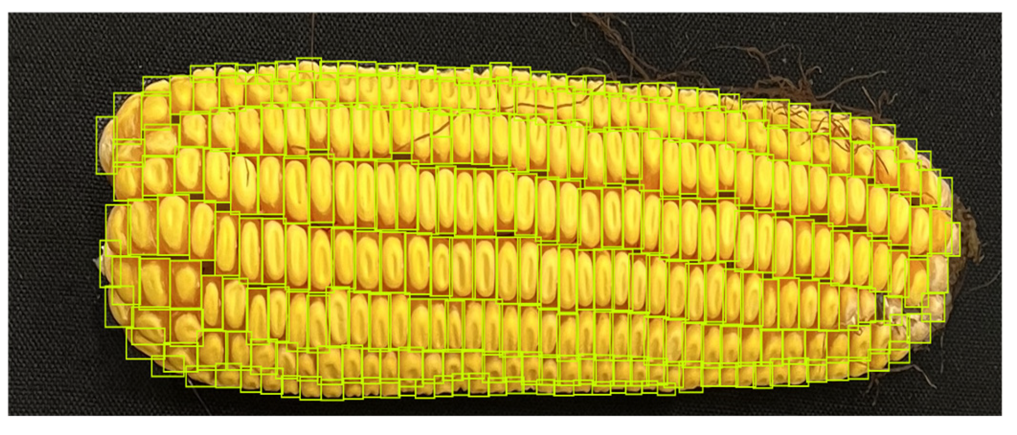
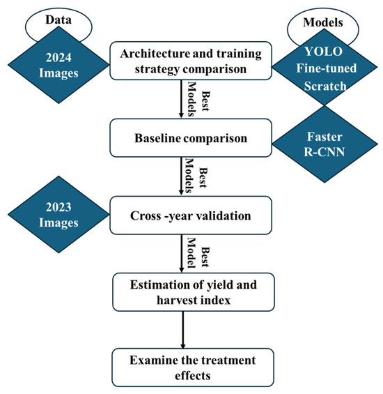
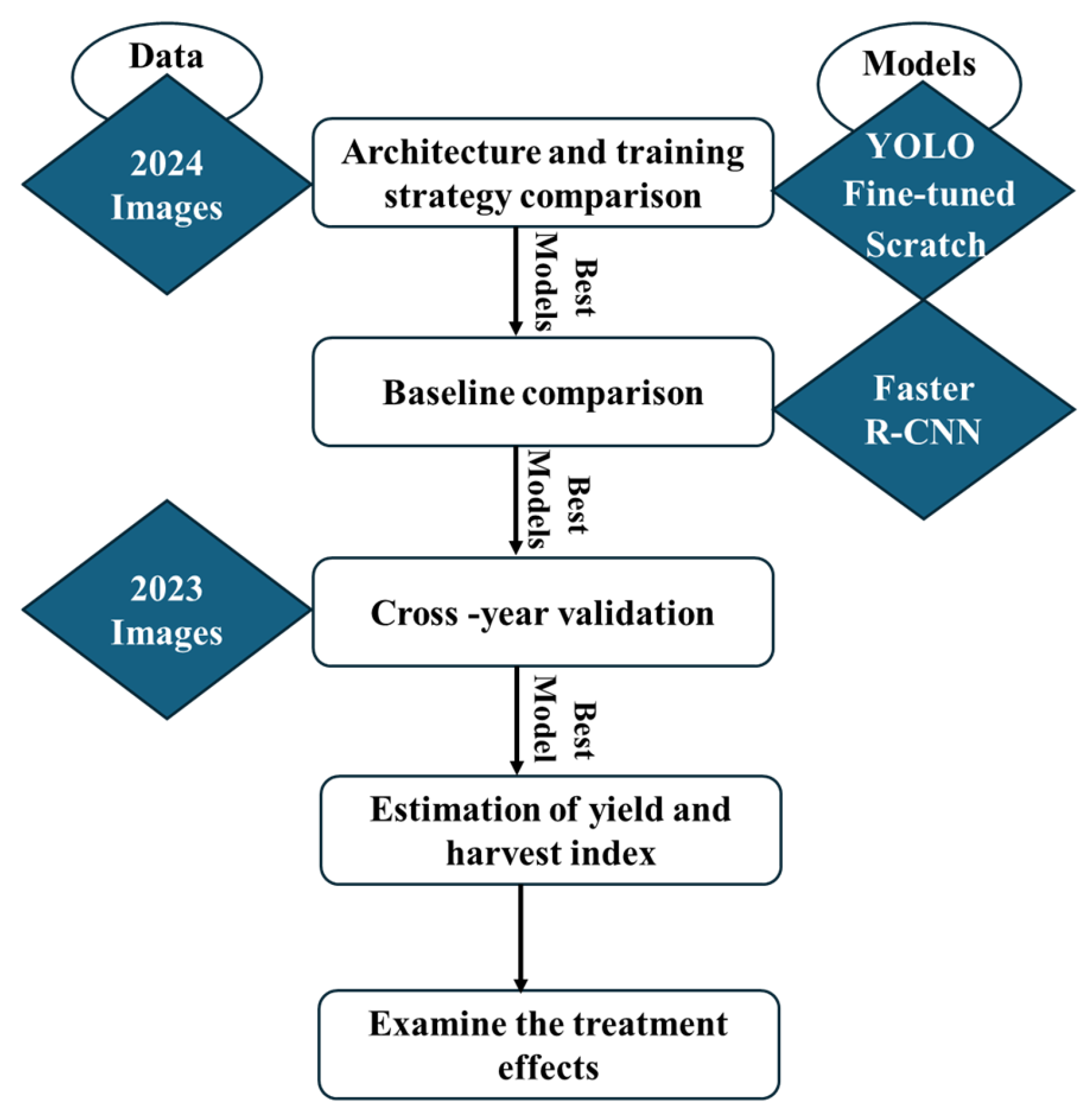
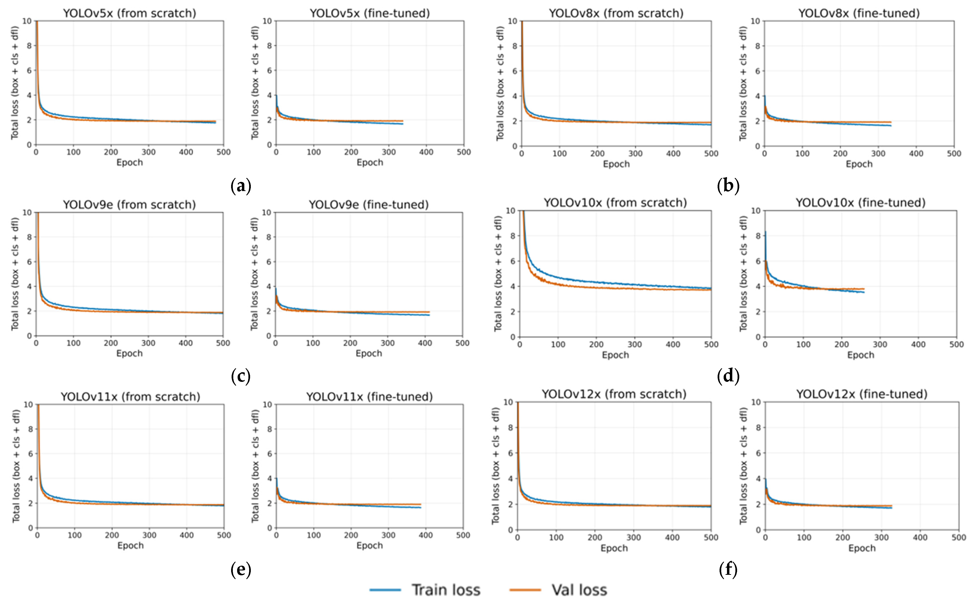
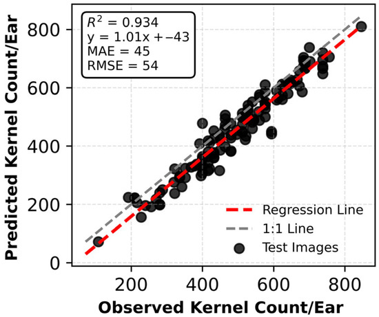
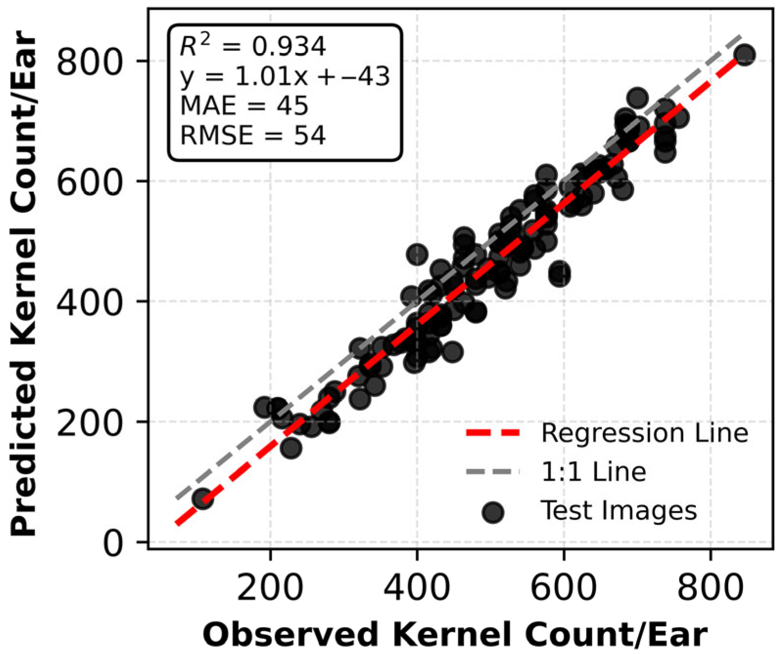
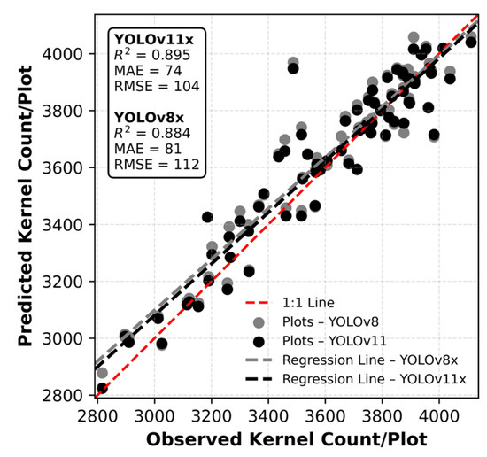
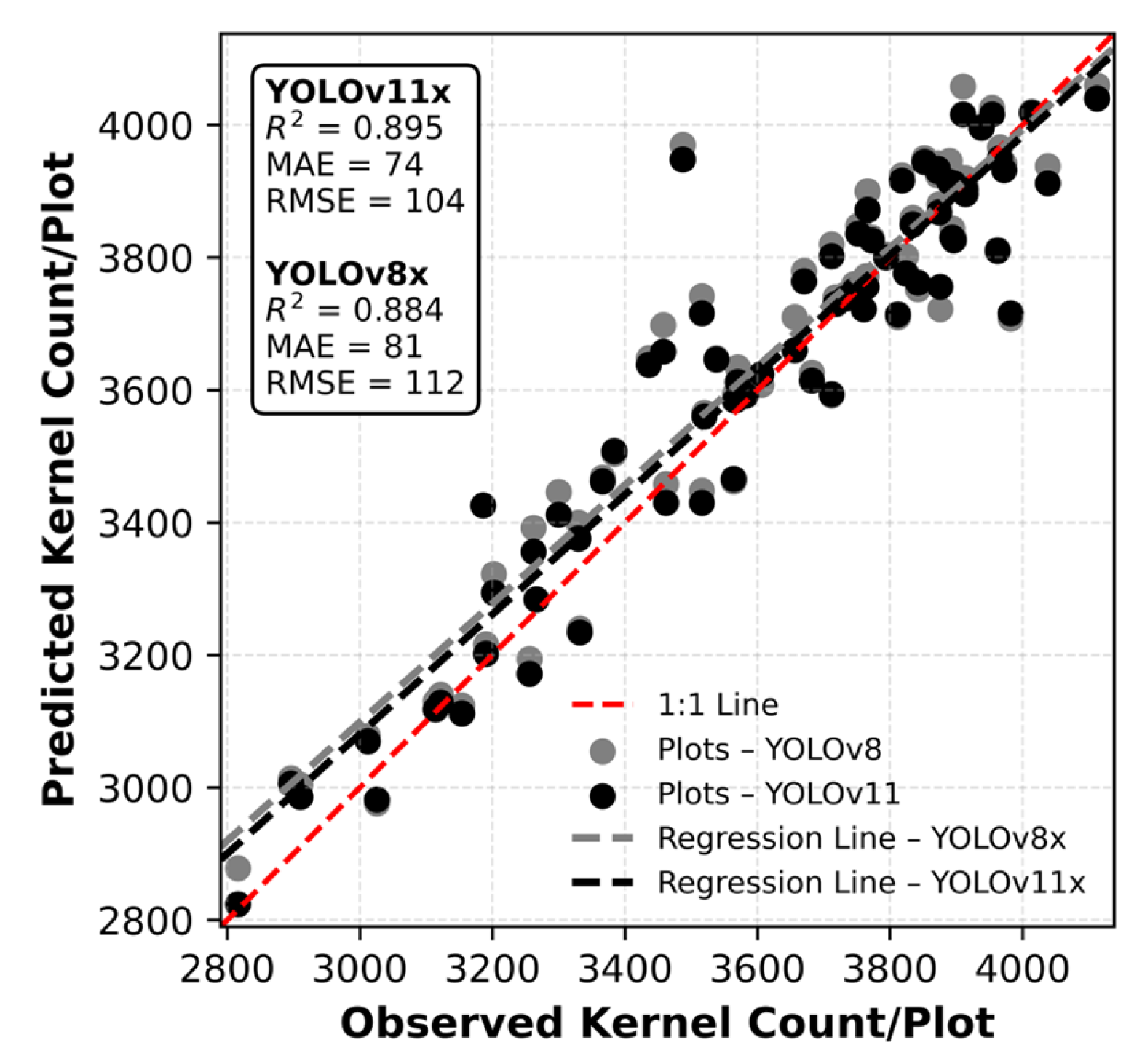
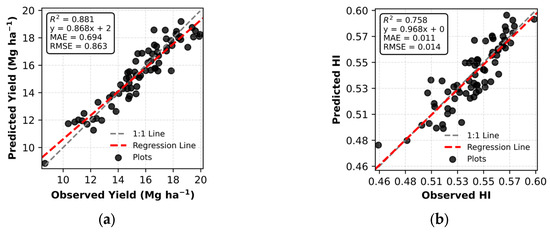
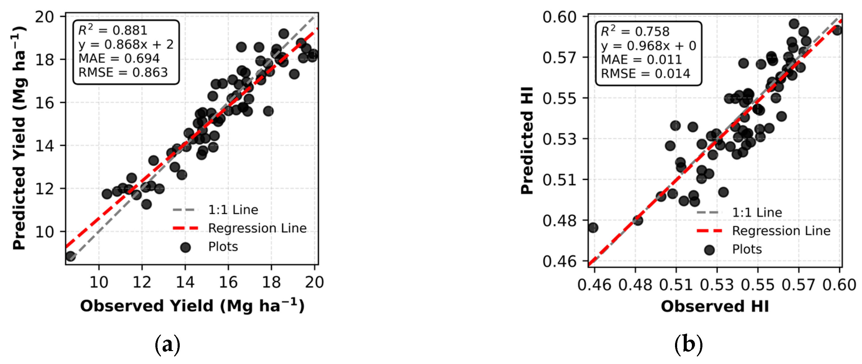
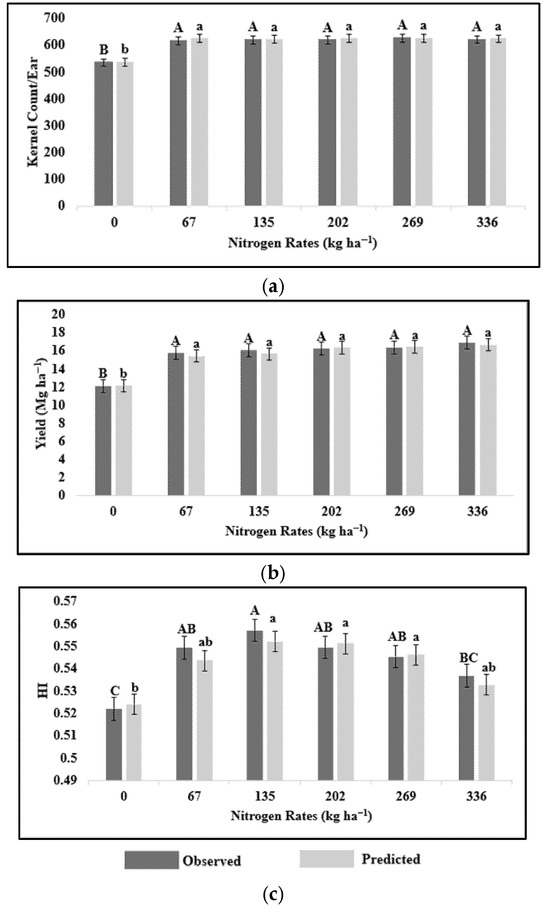
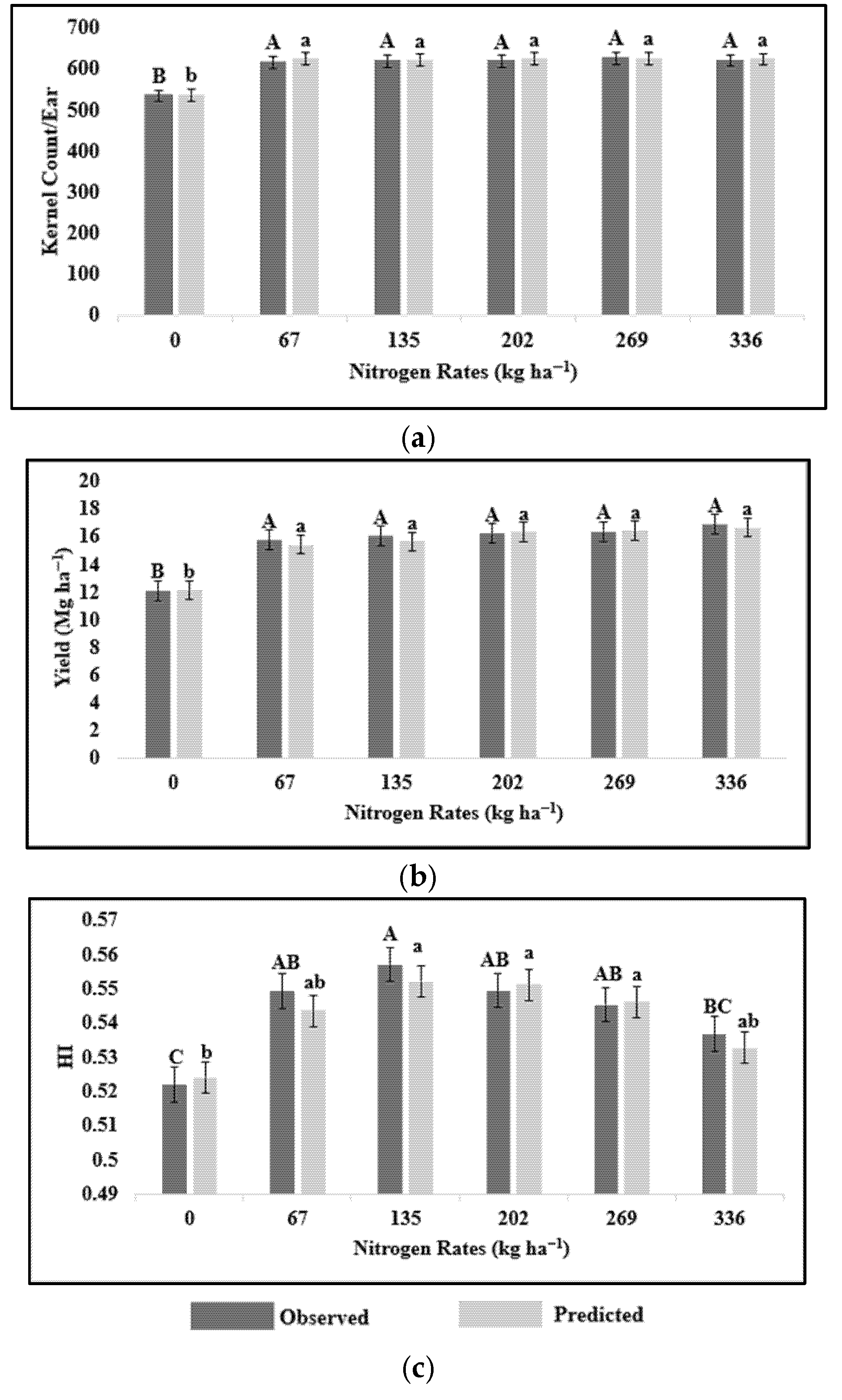

Disclaimer/Publisher’s Note: The statements, opinions and data contained in all publications are solely those of the individual author(s) and contributor(s) and not of MDPI and/or the editor(s). MDPI and/or the editor(s) disclaim responsibility for any injury to people or property resulting from any ideas, methods, instructions or products referred to in the content. |
© 2026 by the authors. Licensee MDPI, Basel, Switzerland. This article is an open access article distributed under the terms and conditions of the Creative Commons Attribution (CC BY) license.