Intelligent Control Framework for Optimal Energy Management of University Campus Microgrid

Highlights

What are the main findings?

• A two-stage energy management framework is proposed, where genetic algorithm (GA) optimization provides an offline reference schedule while reinforcement learning (RL) enables adaptive real-time operation under uncertain and time-varying conditions.
• A penalty breakdown framework is introduced to interpret RL behavior and to explicitly link learned policies to physical and economic drivers such as electricity price, voltage constraints, and battery usage.

What are the implications of the main findings?

• The proposed GA-RL architecture enables scalable and deployable supervisory energy management for smart campus and smart city microgrids.
• The proposed interpretability framework enables systematic reward design and supports practical deployment of RL-based energy management systems in real microgrids.

Abstract

This study proposes a smart energy management framework for a university campus microgrid aimed at reducing dependence on the main power grid and increasing the utilization of photovoltaic (PV) generation under dynamic load and environmental conditions. The core contribution is a two-stage approach that combines a genetic algorithm (GA) for static day-ahead optimization with a soft actor-critic (SAC) reinforcement learning (RL) agent performing adaptive supervisory management of microgrid active and reactive power flows via battery control. The GA provides an optimal reference schedule under forecasted conditions, while the SAC agent is trained on eight representative scenarios derived from measured PV generation and campus load data to adapt battery operation and grid exchange under uncertainty. The results show that the benefit of RL does not lie in reproducing the static GA solution, but in learning economically rationally adaptive behavior. In particular, the SAC agent exploits low-tariff periods and hedges against adverse PV conditions by proactively adjusting battery charging strategies in real time. This adaptive behavior addresses a key limitation of static optimization, which cannot respond to deviations from forecasted operation, and represents the main added value of the proposed framework. From a practical perspective, the GA-SAC architecture operates at a supervisory level with low computational requirements, making it suitable for scalable deployment in smart campus and smart city energy management systems.

1. Introduction

Microgrids are increasingly being seen as a key enabler for integrating renewable energy sources, distributed storage, and flexible loads in a reliable and cost-effective manner (see, e.g., review articles [1,2,3]).

Recent studies highlight that energy management systems (EMSs) in microgrids increasingly rely on optimization methods to schedule storage and grid exchange, but still face challenges related to uncertainty, real-time implementation, and limited integration between scheduling and learning-based controllers [1,2,3,4]. Classical optimization approaches (including Mixed-Integer Linear Programming (MILP) and metaheuristics such as genetic algorithm (GA) [5]) can provide high-quality day-ahead schedules, but they typically rely on forecasts, and their performance can degrade when actual operating conditions deviate from forecast scenarios. Furthermore, these methods often require re-optimization to respond to rapid fluctuations, which can be computationally demanding for real-time operation. In response to these limitations, artificial intelligence (AI)-based EMS solutions, including neural networks (NNs) and reinforcement learning (RL), have been proposed to improve adaptability and reduce the reliance on repeated optimization runs [6,7]. Model-free RL [8] is gaining popularity because it can learn policies directly from interaction data and can be embedded in hierarchical microgrid control architectures [9]. However, many RL-based microgrid studies focus on objectives such as economical dispatch, coordinated operation over time frames, voltage support, frequency regulation, or energy trading [10,11,12,13,14,15,16,17] rather than on photovoltaic (PV)-level [18] Maximum Power Point Tracking (MPPT) as part of an integrated microgrid EMS.

Table 1 presents the above-cited EMS approaches comparing how they apply optimization and learning techniques and highlighting their strengths and their limitations.

Table 1. Energy management system (EMS) approaches (optimization vs. learning).

Category	Representative Works	Strengths	Limitations (Gaps)
Optimization-based EMS (GA/MILP/heuristics)	[2,4,5,19]	High-quality day-ahead schedules; explicit constraints	Forecast-dependent; limited real-time adaptivity; re-optimization cost
Neural network/machine learning-based EMS	[6,7]	Fast inference; reduces repeated Optimal Power Flow/MILP	Needs training dataset; generalization/robustness concerns
Reinforcement learning (RL)-based microgrid operation (including soft actor-critic)	[9,10,11,12,13,14,15,16,17]	Adaptive control; handles uncertainty; model-free options	Often targets cost/voltage/frequency/trading, not photovoltaic (PV) Maximum Power Point Tracking (MPPT) integration

From a PV control perspective, classical MPPT techniques [20] (e.g., extremum search and P&O-based strategies) remain widely used due to their simplicity, but they can exhibit slow tracking or oscillations under rapidly changing irradiance and temperature conditions [21]. GA-based controller tuning has also been investigated to improve MPPT performance and robustness [19], but such approaches typically operate at the controller parameter level and do not provide an adaptive policy that generalizes to different environmental and load scenarios.

Therefore, there remains a gap in combining optimization-based EMS scheduling with RL-based real-time MPPT of PV systems in a unified framework, especially in a realistic campus microgrid environment with heterogeneous loads. The present work fills this gap by integrating GA-based day-ahead scheduling with soft actor-critic (SAC)-based real-time MPPT control and evaluating their complementary roles under multiple generation and load scenarios.

Ref. [22] proposes a WEB-based platform integrating GA optimization, heuristic control, RL, and Long Short-Term Memory (LSTM)-based load forecasting for energy management in microgrids. The role of the adaptive learning-based control for energy management in fluctuating grid conditions is presented.

For the implementation of MPPT optimization, the actor-critic approach is preferred. Since this study is focused on continuous real-time control of MPPT, the most appropriate approach is to apply a soft actor-critic approach.

Table 2 shows how SAC agents are used in other microgrids, compared to the agent’s role in the current study.

Table 2. The SAC agent’s role in microgrids compared to its role in the current work.

Work	Target Objective	Control Level	Uses SAC?	Includes PV MPPT?	Key Difference vs. This Work
[10]	Multi-timescale operation Hybrid Energy Storage System (HESS)	Energy management system (EMS) real-time correction	Yes	No	Focuses on HESS deviations; not photovoltaic (PV) Maximum Power Point Tracking (MPPT) policy
[11]	Voltage support	Power quality	Yes	No	Energy storage system (ESS) voltage control; not PV energy extraction
[13]	Generation cost	Distributed EMS	Yes	No	Economic dispatch focus
[14]	Energy trading resilience	Networked microgrids	Yes (LSTM-SAC)	No	Trading and resilience focus
This paper	PV MPPT + EMS scheduling	PV control + day-ahead plan	Yes	Yes	Unified GA scheduling + SAC MPPT in campus microgrid

Existing hybrid GA-NN and GA-RL microgrid EMS schemes typically use the GA either to generate training labels for supervised learning or to initialize RL policies, with the objective of approximating the same optimization solution.

In contrast, the new intelligent control framework proposed in this study deliberately decouples GA planning and RL control. The GA provides an offline optimal reference and cost structure, while the SAC agent learns an autonomous policy with a different objective function, emphasizing price awareness and voltage smoothness under uncertainty. This design enables a meaningful comparison between static optimization and learned adaptive behavior, rather than imitation or surrogate optimization. The proposed framework combines (i) static day-ahead optimization of energy planning using the GA [5] and (ii) online adaptive control using an SAC agent trained by RL [8] to improve real-time performance. The GA component calculates an optimized battery charging/discharging schedule and grid power profile under predicted scenarios, with the aim of minimizing grid dependency and improving energy autonomy. In parallel, the SAC agent is trained to perform real-time Maximum Power Point Tracking of the PV subsystem by continuously adapting the duty cycle of the direct current (DC)–DC converter under different irradiation, temperature, and load conditions. Similar positioning of RL as a surrogate or complement to optimization-based EMS has been reported in recent studies, such as [23].

The main novelty of the proposed approach lies in the unified integration of GA-based scheduling and SAC-based real-time MPPT in a campus microgrid environment, which allows for the evaluation of how a learned policy can approximate or complement static optimization under different operational scenarios. PV MPPT is treated as an integral component of the supervisory EMS rather than as a standalone control problem. The framework is validated on a university campus microgrid consisting of four interconnected buildings with heterogeneous loads, including laboratory facilities with active and reactive power consumption (the “University for Business and Technology” (UBT) college in Pristina, Kosovo, (https://www.ubt-uni.net/en/home/, accessed on 1 September 2025)). University campus microgrids represent a scaled and realistic proxy for smart district and smart city energy systems, where uncertainty, heterogeneity of loads, and real-time adaptability are critical. The obtained results demonstrate improved energy utilization and reduced grid dependency, highlighting the potential of hybrid optimization and RL strategies for practical microgrid control.

Accordingly, this paper focuses on the complementary roles of static optimization and adaptive RL, rather than on developing new optimization heuristics or MPPT algorithms in isolation.

The rest of the paper is organized as follows: Section 2 presents the microgrid setup and describes the methodology of this study; Section 3 presents the experimental results obtained; Section 4 includes a discussion on the results; and Section 5 presents conclusions, as well as some limitations and future research directions.

2. Microgrid Setup and Methodology

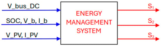
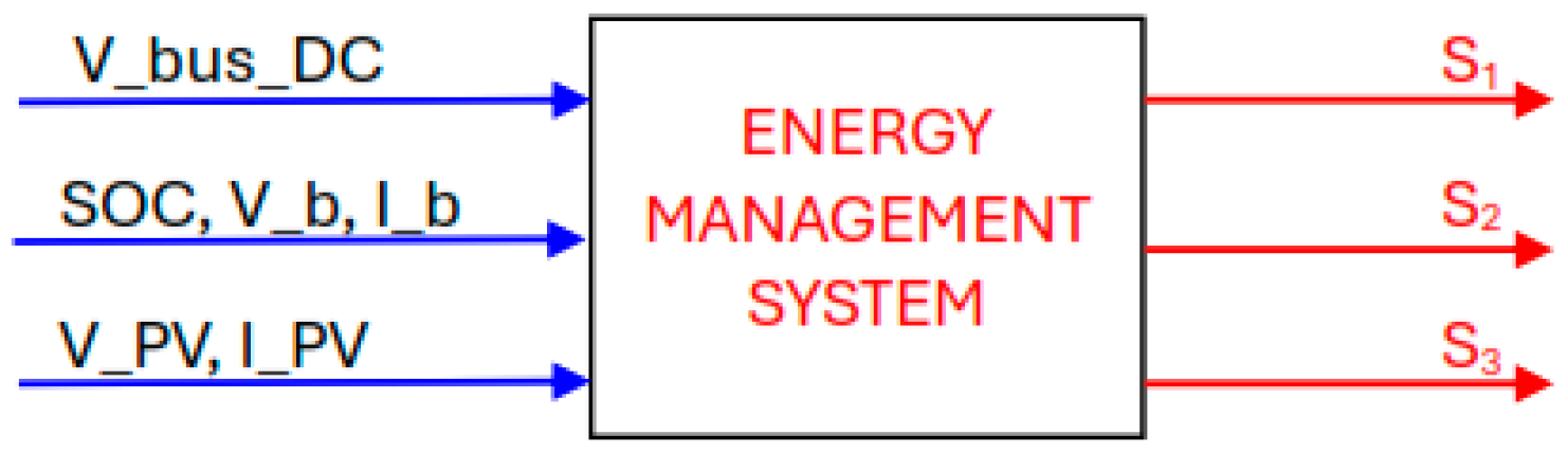
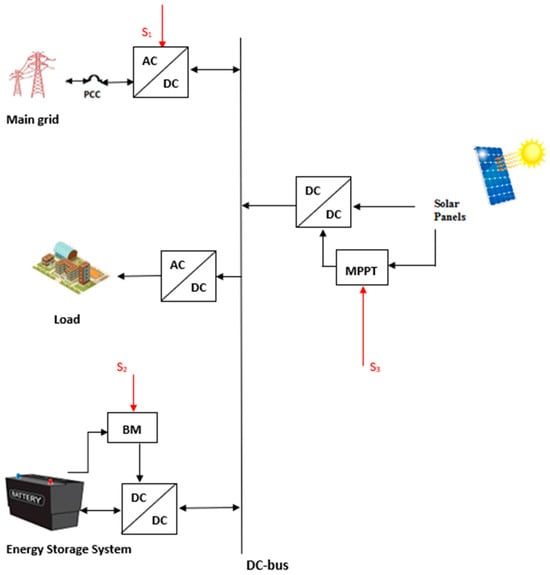
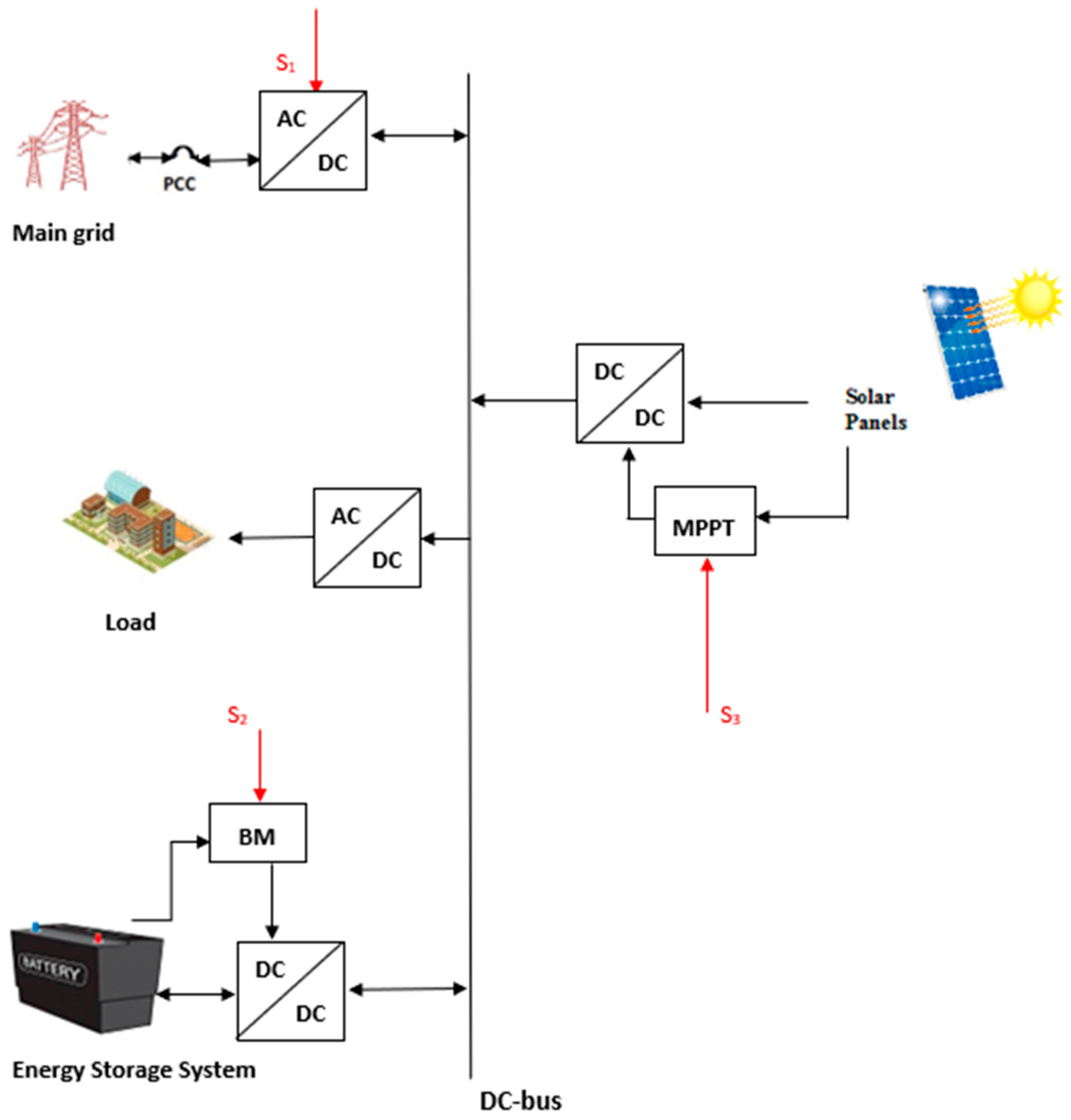
The microgrid considered in the current study is the main connected grid. It includes buildings, a PV system, a battery energy storage (BES) system, and an EMS. The EMS performs real-time energy control, sending signals S₁, S₂, and S₃ corresponding to the Point of Common Coupling (PCC); battery management (BM) of the BES system; and the MPPT of the PV system (Figure 1 and Figure 2).

Figure 1. EMS scheme.

Figure 2. DC bus-based microgrid architecture.

The EMS sends signals for the optimal management of the PV system in MPPT mode. It also regulates the charging/discharging schedule of the BES system. The aim is to achieve good power balance in the microgrid and to minimize the amount of energy consumed from the main grid. Figure 1 presents the scheme with the input and output signals of the EMS.

SOC denotes the state of charge of the BES system, V_bus_DC is the value of the DC bus voltage, V_b and I_b are the energy storage system (ESS) input signals from the BES system, and V_PV and I_PV are the input signals from the PV system.

Figure 2 illustrates a DC bus-based microgrid architecture enabling unified integration of PV generation, battery storage, and grid connection through an alternating current (AC)/DC interface. The red arrows indicate the control signals coming from the EMS.

The methodology applied in this study is presented below.

The Simulink model is developed using average-value representations of the main microgrid components, which is appropriate for supervisory energy management and RL studies at hourly time scales. The PV array is modeled using an irradiance- and temperature-dependent power characteristic, while the DC–DC and AC/DC converters are represented by averaged power-flow models without explicit switching dynamics. The battery energy storage system is modeled using an SOC-based energy model with power and operational constraints. Grid interaction at the PCC is represented using a Thévenin equivalent. This modeling approach allows for efficient simulation of long-term scenarios and focuses the analysis on system-level energy flows rather than high-frequency switching losses.

2.1. Objective and General Design

This study develops and evaluates a two-stage microgrid optimization and control methodology that combines (i) static day-ahead optimization using the GA and (ii) adaptive control using an SAC RL agent. The main objective is to reduce dependence on the main grid while ensuring operational feasibility and power quality compliance by jointly considering active and reactive power exchange, SOC stability, and voltage regulation under renewable and load variability.

2.2. Conceptual Framework and Modeling Levels

The proposed framework follows a standard three-layer hierarchical control architecture. The physical simulation layer represents the microgrid dynamics and network constraints. The optimization layer employs the GA to compute an offline, scenario-dependent optimal reference policy. The training and control layer use an SAC agent operating at a supervisory EMS level to provide adaptive real-time control under uncertainty.

The proposed framework consists of three interacting layers:

• Physical simulation layer: A microgrid model with PV generation, battery storage, loads, and grid interface, driven by 24 h demand, temperature, and solar radiation profiles.
• Optimization layer (GA): Calculation of an “ideal” static policy for a given scenario, generating reference trajectories for the SOC and grid exchange.
• Training and control layer (SAC): Offline training of a model-free RL agent by interacting with the simulated environment, with a reward structure shaped to encourage policies consistent with the optimization objectives and operational constraints.

The GA solution serves as a reference baseline and supports reward shaping and diagnostic comparisons between static and learned policies.

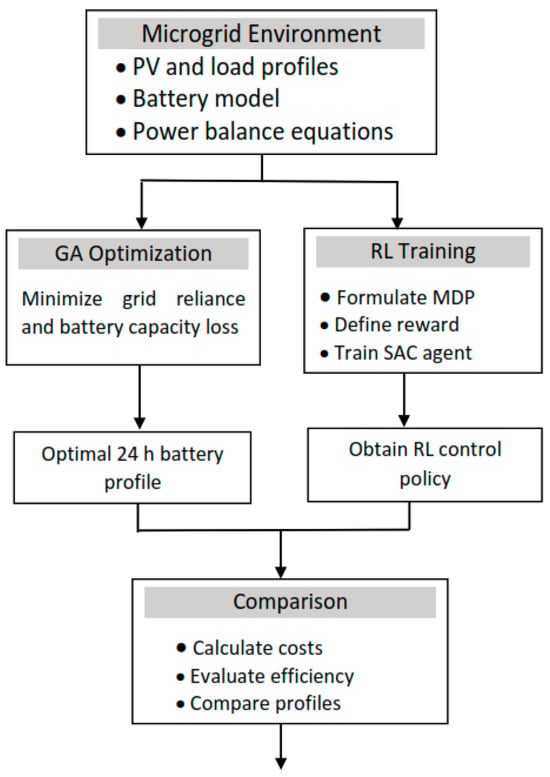
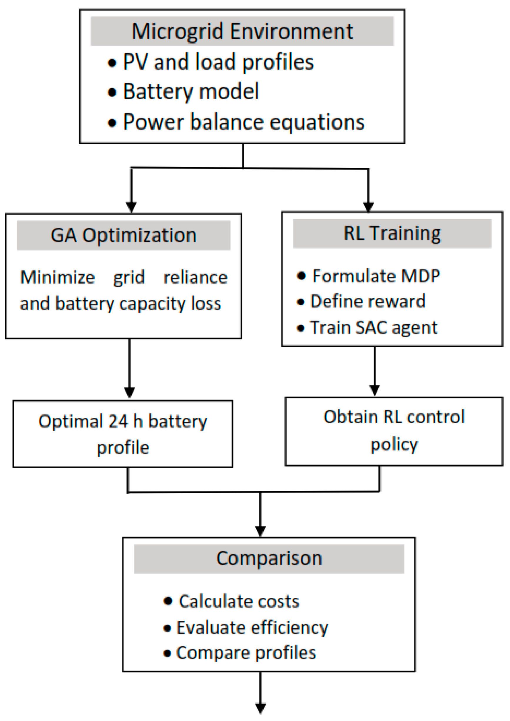
A flowchart of the methodology is presented in Figure 3.

Figure 3. Flowchart of implemented methodology.

2.3. Modeling the Microgrid Environment

Campus loads are modeled with both active and reactive power components, reflecting the presence of information technology (IT) equipment, laboratory devices, and auxiliary systems.

In the presence of reactive power, the total apparent power of the building is calculated as follows:

$$S(t) = \sqrt{{P(t)}^2+{Q(t)}^2}$$

(1)

where

P(t) is the active power (real consumption);

Q(t) is the reactive power (influence from computers, Uninterruptible Power Supply (UPS), etc.).

The power factor pf is calculated as follows:

$$pf = \cos (\phi ) = {\displaystyle \frac{P(t)}{S(t)}}$$

(2)

For a campus with mixed loads, often cos(φ) = 0.9.

In cases where data on the consumed active power in the microgrid P_load(t) are available, the reactive power in the microgrid is calculated as follows:

Q_load(t) = P_load(t)·tan(arccos(0.9))

(3)

For the experimental calculations, a constant power factor of cos(φ) = 0.95 is assumed to represent a typical mixed campus load.

At the PCC level, complex power is used:

S(t) = P(t) + jQ(t)

(4)

The power balance is defined as follows:

P_grid(t) = P_load(t) − P_pv(t) − P_bat(t)

(5)

and

Q_grid(t) = Q_load(t) − Q_pv(t) − Q_bat(t),

(6)

where P_bat(t) and Q_bat(t) are the controlled signals from the agent. In our case, Q_pv(t) = 0.

2.4. Static Optimization via GA

The GA is used to identify the optimal daily battery power profile Pbat(t), t = 1, …, 24 that minimizes the overall grid dependency and losses from inefficient capacity utilization. Let the battery capacity be denoted by C_bat,max.

Decision variables:

x = [P_bat,1, P_bat,2, …, P_bat,24]

Let the state of charge, SOC(t), be the energy in the battery [kWh], and Δt be a time interval of one hour [h]. By convention, we have the following:

P_bat,t > 0: battery discharging;

P_bat,t < 0: battery charging;

SOC(t) ∈ [SOC_min, SOC_max].

The SOC is updated according to the following formula:

$$SOC(t + 1) = SOC(t) + {\eta }_{ch}{P}_{ch}(t)\Delta t - {\displaystyle \frac{1}{{\eta }_{ch}}}{P}_{disch}(t)\Delta t,$$

(7)

where Δt = 1 h. It is assumed that P_ch(t) < 0 and P_disch(t) > 0. Charging and discharging at the same time is impossible, i.e., when P_ch(t) ≠ 0, P_disch(t) = 0, and vice versa when P_disch(t) ≠ 0, P_ch(t) = 0.

Constraints:

P_ch(t)P_disch(t) = 0

(8)

$$SOC(t+1)=SOC(t)+{\displaystyle \frac{P_{bat}\left(t\right)\Delta t}{C_{bat,max}}}$$

(9)

SOC_min ≤ SOC(t) ≤ SOC_max

(10)

and

$$|P_{bat}(t)| \le P_{bat,max}, P_{bat}(t{)}^2+Q_{bat}(t{)}^2 \le S_{bat,max}^2$$

(11)

Ultimately, we obtain the following:

$${\sum }_{t=1}^{24}{P}_{bat}\left(t\right)=0; t=1,\dots ,24$$

(12)

SOC_min and SOC_max in Equation (10) are fixed at 20% and 100% of C_bat,max, respectively.

The constraint in (12) ensures the same value of the SOC at the end of the 24 h period as at the beginning of that period (SOC(0) = SOC(24)). SOC(1) and SOC(24) are fixed at 50% of C_bat,max.

Power factor requirement in PCC (by grid code):

Minimum pf_min ∈ (0, 1] ⇒ allowable Q_grid:

|Q_grid(t)| ≤ tan(arccos(pf_min))|P_grid(t)|

(13)

In the case of a hard limit,

|Q_grid(t)| ≤ Q_grid,max.

(14)

A linear model (LinDistFlow/Thévenin) for the voltage at the PCC:

The per-unit (p.u.) approximation [24,25] is as follows:

$$V_{\mathrm{pcc}}(t)\approx V_0 - {\displaystyle \frac{R_{\mathrm{t}\mathrm{h}}{P}_{\mathrm{g}\mathrm{r}\mathrm{i}\mathrm{d}}\left(t\right)+ X_{\mathrm{t}\mathrm{h}}{Q}_{\mathrm{g}\mathrm{r}\mathrm{i}\mathrm{d}}\left(t\right) }{V_{\mathrm{b}\mathrm{a}\mathrm{s}\mathrm{e}}}}$$

(15)

where $R_{\mathrm{t}\mathrm{h}}$ and $X_{\mathrm{t}\mathrm{h}}$ are “equivalent” resistances/reactances between the PCC and a harder point of the grid (they can be parameters of the environment). V_base is the nominal voltage in the PCC. Equation (15) can be presented in the following form:

$$V_{\mathrm{p}\mathrm{c}\mathrm{c}}^{\mathrm{p}\mathrm{u}}(t)\approx 1 - ({\mathrm{R}}^{\prime }{P}_{\mathrm{g}\mathrm{r}\mathrm{i}\mathrm{d}}^{\mathrm{p}\mathrm{u}}(t)+ \mathrm{X}\prime Q_{\mathrm{g}\mathrm{r}\mathrm{i}\mathrm{d}}^{\mathrm{p}\mathrm{u}}(t))$$

(16)

where

$$P_{\mathrm{g}\mathrm{r}\mathrm{i}\mathrm{d}}^{\mathrm{p}\mathrm{u}}(t)={\displaystyle \frac{P_{\mathrm{g}\mathrm{r}\mathrm{i}\mathrm{d}}\left(t\right)·{10}^3}{S_{\mathrm{b}\mathrm{a}\mathrm{s}\mathrm{e}}}}$$

(17)

$$Q_{\mathrm{g}\mathrm{r}\mathrm{i}\mathrm{d}}^{\mathrm{p}\mathrm{u}}(t)={\displaystyle \frac{Q_{\mathrm{g}\mathrm{r}\mathrm{i}\mathrm{d}}\left(t\right)·{10}^3}{S_{\mathrm{b}\mathrm{a}\mathrm{s}\mathrm{e}}}}$$

(18)

R′ and X′ are sensitivities (dimensionless). 0.95 ≤ $V_{\mathrm{p}\mathrm{c}\mathrm{c}}^{\mathrm{p}\mathrm{u}}(t)$ ≤ 1.05.

The Thévenin equivalent parameters R′ and X′ [24] represent the aggregated upstream network impedance at the PCC and are selected within typical ranges for low-voltage campus feeders. $R^{\prime }\in [0.01,0.1]$ p.u. and $X^{\prime }\in \left[\mathrm{0.02,0.3}\right]$ p.u., resulting in an $X^{\prime }/R^{\prime }$ ratio between 1 and 5.

S_base is the microgrid rating.

This model captures the first-order dependence of voltage on power flow and is accurate enough for operational optimization and voltage penalties.

Price profile (day/night) and asymmetry purchasing ↔ selling

The hourly purchase price C_buy(t) is 0.124 USD/kWh for 06:00–21:59 and 0.062 USD/kWh for 22:00–05:59 (in the code: night hours 22, 23, 0–6) [26].

There is no FiT (feed-in tariff) as resale does not bring in revenue. To prevent “excessive resale”, we impose asymmetric weights as follows:

• A heavier penalty for positive P⁺_grid (purchasing energy from the main grid);
• A lighter penalty for negative P⁻_grid (resale/selling energy to the main grid).

The objective function to be minimized is as follows:

$$\begin{gathered} J_{\mathrm{GA}}={\sum }_{t=1}^{24}\left[C_{\mathrm{b}\mathrm{u}\mathrm{y}}\left(t\right)\left(w_{\mathrm{P}+}{\left[P_{grid}^{+}\left(t\right)\right]}^2\right)+\left(w_{\mathrm{P}-}{\left[P_{grid}^{-}\left(t\right)\right]}^2\right)+w_Q\max {\left({0,|Q}_{grid}\left(t\right)|-Q_{\mathrm{g}\mathrm{r}\mathrm{i}\mathrm{d},\mathrm{l}\mathrm{i}\mathrm{m}}\left(t\right)\right)}^2+ \\ {w}_{SOC}{\left[(SOC\left(t\right)-{SOC}_{\mathrm{t}\mathrm{a}\mathrm{r}\mathrm{g}\mathrm{e}\mathrm{t}}\left(t\right)\right]}^2+w_V\varphi \left(V_{\mathrm{p}\mathrm{u}}\left(t\right)\right)+w_{\Delta V}{\left({\displaystyle \frac{{\Delta \mathrm{V}}_{\mathrm{p}\mathrm{u}}\left(t\right).}{V_{\mathrm{s}\mathrm{c}\mathrm{a}\mathrm{l}\mathrm{e}}}}\right)}^2\right] \end{gathered}$$

(19)

The objective function includes weighted quadratic penalties for grid purchasing and selling, reactive power violations, SOC deviation from a target profile, voltage deadband violations, and voltage smoothness. The weighting coefficients control the trade-off between economic efficiency, power quality, and battery health: w_P is the active power coefficient (usually = 1); w_Q is the reactive power coefficient; w_SOC is the charge stability coefficient for SOC smoothness (usually = 0.05); SOC_target(t) is the desired SOC profile (it could be flat or set according to an energy plan); $P_{\mathrm{g}\mathrm{r}\mathrm{i}\mathrm{d}}^{+}\left(t\right)$ = max($P_{grid}\left(t\right), 0$) (purchasing); and $P_{\mathrm{g}\mathrm{r}\mathrm{i}\mathrm{d}}^{-}\left(t\right)$ = max(${-P}_{grid}\left(t\right), 0$) (selling); and $\varphi (V)$ is a hinge with “deadband”, where V ∈ [V_min, V_max]. According to the European requirements for LV/MV systems and the ENTSO-E network codes [27], the time of microgrid voltage outside the deadband should be 0.0%.

The GA optimization stage adopts a day-ahead operating strategy by minimizing the objective function $J_{GA}$ in Equation (19) over a 24 h horizon, subject to the operational constraints defined in Equations (8)–(12). The objective includes quadratic penalties for (1) grid purchasing $P_{grid}^{+}(t)$, weighted by the time-varying energy price $c_{buy}(t)$; (2) grid selling $P_{grid}^{-}\left(t\right),$ avoiding non-physical “pumping” effects when feed-in incentives are absent; (3) reactive power limit violations through $\mathrm{m}\mathrm{a}\mathrm{x}(0,\mid Q_{grid}(t)\mid -Q_{grid,lim}(t){)}^2$; (4) SOC tracking relative to a desired SOC profile $SO{C}_{target}(t)$, promoting daily balance and avoiding unhealthy end-of-day deep cycles; (5) voltage compliance via a hinge (deadband) penalty $\varphi (V_{\mathrm{p}\mathrm{u}}\left(t\right))$, enforcing operation within $\left[V_{min},V_{max}\right]$; and voltage smoothness via an anti-flicker term $w_{\Delta V}{\left({\displaystyle \frac{{\Delta \mathrm{V}}_{\mathrm{p}\mathrm{u}}\left(t\right).}{V_{\mathrm{s}\mathrm{c}\mathrm{a}\mathrm{l}\mathrm{e}}}}\right)}^2$.

The coefficients $w_P,w_Q,w_{SOC},w_V,$ and $w_{\Delta V}$ control the trade-off between grid exchange minimization, reactive compliance, SOC stability, and voltage quality.

The term $C_{\mathrm{b}\mathrm{u}\mathrm{y}}\left(t\right)\left(w_{\mathrm{P}+}{\left[P_{\mathrm{g}\mathrm{r}\mathrm{i}\mathrm{d}}^{+}\left(t\right)\right]}^2\right)$ directs the battery to reduce purchases, especially during “expensive” hours. The square stabilizes optimization and makes large purchases unattractive.

The term $w_Q\max {\left({0,|Q}_{\mathrm{g}\mathrm{r}\mathrm{i}\mathrm{d}}\left(t\right)|- Q_{\mathrm{g}\mathrm{r}\mathrm{i}\mathrm{d},\mathrm{l}\mathrm{i}\mathrm{m}}\left(t\right)\right)}^2$ penalizes the deviation of the reactive power from its limit.

The term $w_{\mathrm{P}-}{\left[P_{\mathrm{g}\mathrm{r}\mathrm{i}\mathrm{d}}^{-}\left(t\right)\right]}^2$ slightly discourages selling to the main grid when there is no FiT, preventing “pumping” to reduce J_GA.

The term $w_{SOC}{\left[(SOC\left(t\right)-{SOC}_{\mathrm{t}\mathrm{a}\mathrm{r}\mathrm{g}\mathrm{e}\mathrm{t}}\left(t\right)\right]}^2$ ensures daily balance and a healthy SOC profile (without deep cycles towards the end of the day).

The term $w_V\varphi \left(V_{\mathrm{p}\mathrm{u}}\left(t\right)\right)$ provides a hard priority for safety/voltage compliance; 0% in the deadband is the desired behavior.

The term $w_{\Delta V}{\left({\displaystyle \frac{{\Delta \mathrm{V}}_{\mathrm{p}\mathrm{u}}\left(t\right).}{V_{\mathrm{s}\mathrm{c}\mathrm{a}\mathrm{l}\mathrm{e}}}}\right)}^2$ smooths the voltage (anti-flicker) and limits rapid jumps, which is beneficial for the equipment and for the comfort of the grid.

Static optimization by means of the GA in (19) subject to the constraint system ((8)–(12)) is used to ensure “ideal” policies. The optimal solutions obtained are used for reward shaping in the RL model.

2.5. Parameter Selection and Robustness

The weighting coefficients in the GA objective function (${\mathrm{w}}_{{\mathrm{P}}^{+}},{\mathrm{w}}_{{\mathrm{P}}^{-}},{\mathrm{w}}_{\mathrm{Q}},{\mathrm{w}}_{\mathrm{S}\mathrm{O}\mathrm{C}},{\mathrm{w}}_{\mathrm{V}},{\mathrm{w}}_{\Delta \mathrm{V}}$) are selected to reflect operational priorities rather than to achieve numerical optimality. Higher weights are assigned to grid power exchange and SOC constraint violations to ensure feasibility and battery health, while voltage-related penalties are used to enforce power quality compliance. The selected values lie within commonly adopted ranges, and empirical tests confirmed stable behavior under moderate parameter variations.

Importantly, the proposed framework does not rely on a single fixed operating point. The SAC agent is trained on multiple scenarios with varying generation and load conditions, which promotes policy robustness and reduces sensitivity to moderate variations in weighting coefficients and SOC bounds.

2.6. Concept and Function of SAC Agent

The SAC is an off-policy actor-critic algorithm with entropy regularization, providing stable learning and effective exploration in continuous action spaces.

The SAC agent consists of an actor network generating continuous control actions (π) and two critic networks estimating action values to mitigate overestimation bias.

State space:

At each decision step $t$, the agent observes the normalized state vector:

$$s_t=\left[P_{pv}^{norm}(t), P_{load}^{norm}(t), Q_{load}^{norm}(t), SO{C}_{norm}(t), Hou{r}_{norm}(t)\right],$$

where the normalization ensures bounded inputs and stable learning. The inclusion of the hour index allows the agent to implicitly learn time-dependent patterns in generation, load, and pricing.

Action space:

The continuous action vector is defined as follows:

$$a_t=\left[P_{bat}^{norm}(t), Q_{bat}^{norm}(t)\right]\in {[-1, 1]}^2$$

where the actor directly regulates the battery’s active power (charging/discharging) and reactive power compensation. PV generation is not directly controlled by the agent; instead, its impact is reflected in the power balance and grid exchange.

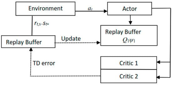
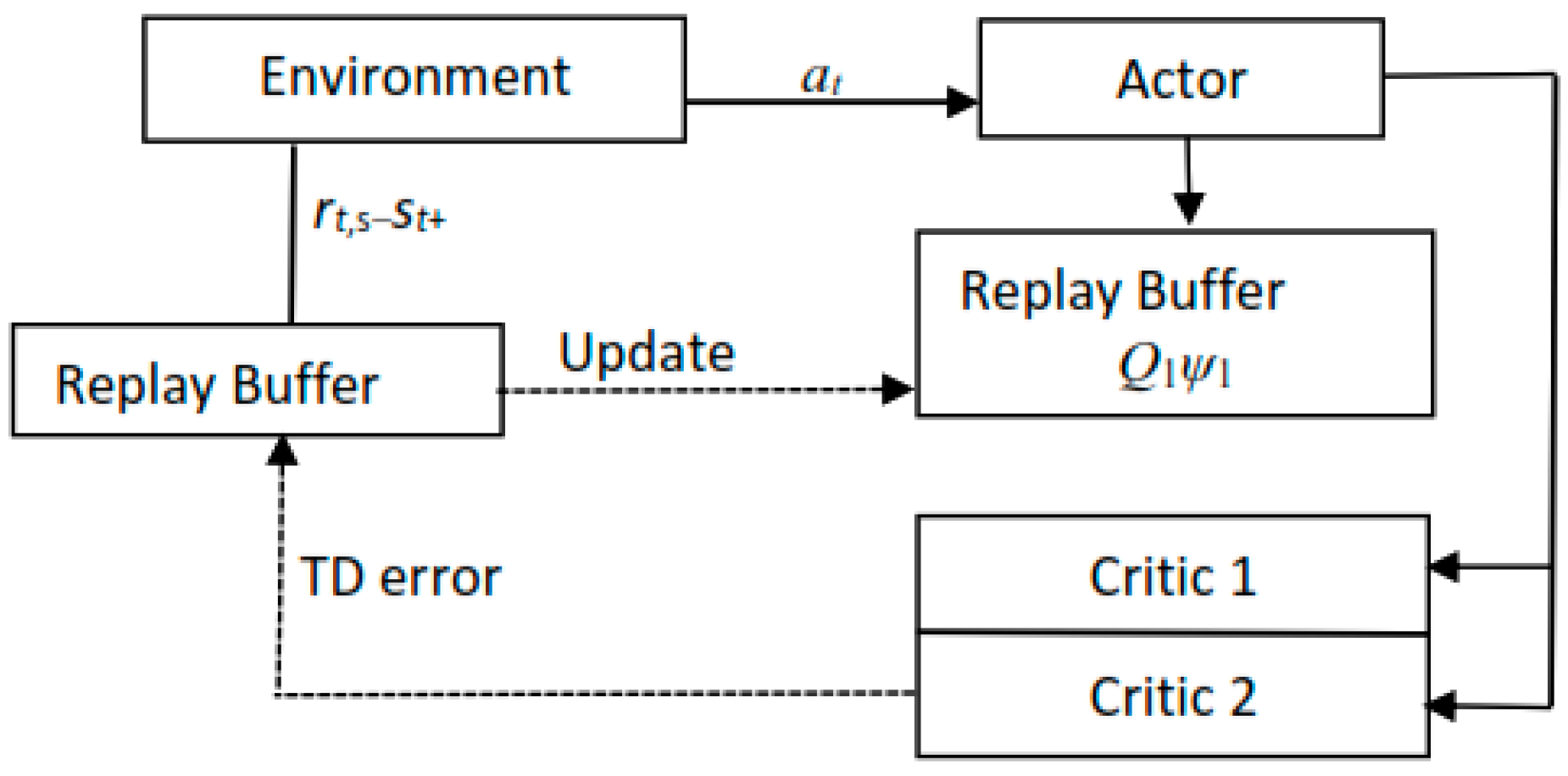
At each step, the agent observes the system’s state, selects a control action, and updates its policy based on the reward received.

A flowchart of the SAC agent is presented in Figure 4.

Figure 4. Flowchart of SAC agent.

In this study, the actor regulates P_bat and Q_bat (charging/discharging, compensation). Critics (Q₁, Q₂) evaluate how “good” this strategy is while considering the reward, SOC, and exchange with the network. After enough episodes (in our case 350), the actor learns to choose actions that minimize the quadratic cost in reward, i.e., to maintain an SOC close to 0.5. C_bat,max and minimum power exchange with the main grid P_grid, ensuring optimal energy balance.

It is important to distinguish between MPPT control and supervisory energy management. The MPPT controller operates at the DC–DC converter level and is solely responsible for maximizing the active power extracted from the PV system. Reactive power management is not part of the MPPT layer. Instead, reactive power flow and power factor regulation are explicitly addressed at the EMS level through the SAC agent, which controls the active and reactive power of the battery inverter and limits reactive power exchange with the main grid via dedicated penalty terms.

2.7. RL—Training of the SAC Agent

The real-time control problem of the microgrid is formulated as a Markov Decision Process (MDP), where the SAC agent learns a control policy π through offline interaction with a simulated environment. Training is conducted using the MATLAB (R2023b) Reinforcement Learning Toolbox over 250–1000 episodes, with each episode consisting of 24 discrete time steps (Δt = 1 h), corresponding to a full daily operation cycle.

• Environmental dynamics:

The active and reactive power exchange with the main grid are computed as follows:

P_grid(t) = P_load(t) − P_pv(t) − P_bat(t),

Q_grid(t) = Q_load(t) − Q_bat(t) (here, Q_pv(t) = 0);

with P⁺ = max(P_grid(t),0) and P⁻ = max(−P_grid(t),0).

A time-varying electricity price $c\left(t\right)$ is applied, reflecting higher tariffs during daytime hours. Grid code compliance is enforced through limits on the power factor and voltage magnitude at the PCC.

$$\mathrm{Price} c(t)=\left\{\begin{array}{c}0.062{\displaystyle \frac{\$}{\mathrm{k}\mathrm{W}\mathrm{h}}}, t \left[22:00, 6:00\right]\\ 0.124 {\displaystyle \frac{\$}{\mathrm{k}\mathrm{W}\mathrm{h}}} \mathrm{otherwise}\end{array}\right\}$$

(20)

The hourly rate for electricity is denoted by TOU = “Time-of-Use” price. In Equation (26), “TOU price” is the array c(t) [USD/kWh] for each hour t = 1, …, 24;

PF limit: |Q_grid(t)| ≤ tan(arccos(pf_min))|P_grid(t)|

Violation Q_viol = max{|Q_grid(t)| − tan(arccos(pf_min)) |P_grid(t)|, 0}

For each step t, a voltage term $V_{\mathrm{p}\mathrm{u}}\left(t\right)$ (per-unit) is added, which corresponds to $V_{\mathrm{p}\mathrm{c}\mathrm{c}}^{\mathrm{p}\mathrm{u}}(t)$ in (16). It is useful to work with a deadband (e.g., [Vmin, Vmax] = [0.95, 1.05] pu) as only deviations outside the allowable zone are penalized. At the Point of Common Coupling,

$$V_{\mathrm{p}\mathrm{u}}\left(t\right)=1-({\mathrm{R}}^{\prime }{P}_{\mathrm{p}\mathrm{u}}(t)+\mathrm{X}\prime Q_{\mathrm{p}\mathrm{u}}(t),$$

(21)

$$P_{\mathrm{p}\mathrm{u}}(t)={\displaystyle \frac{P_{\mathrm{g}\mathrm{r}\mathrm{i}\mathrm{d}}\left(t\right)·{10}^3}{S_{\mathrm{b}\mathrm{a}\mathrm{s}\mathrm{e}}}},$$

(22)

$$Q_{\mathrm{p}\mathrm{u}}(t)={\displaystyle \frac{Q_{\mathrm{g}\mathrm{r}\mathrm{i}\mathrm{d}}\left(t\right)·{10}^3}{S_{\mathrm{b}\mathrm{a}\mathrm{s}\mathrm{e}}}}.$$

(23)

Here, S_base is the microgrid rating.

Deadband:

$${\varphi }_V(V)= \left\{\begin{array}{c}{\left(V-V_{\mathrm{m}\mathrm{a}\mathrm{x}}\right)}^2, V> V_{\mathrm{m}\mathrm{a}\mathrm{x}}\\ {\left(V_{\mathrm{m}\mathrm{i}\mathrm{n}}-V\right)}^2, V< V_{\mathrm{m}\mathrm{i}\mathrm{n}}\\ 0, \mathrm{otherwise}\end{array}\right\}$$

(24)

Smoothness:

$$\Delta V = V_{\mathrm{p}\mathrm{u}}\left(t\right)-V_{\mathrm{p}\mathrm{u}}\left(t-1\right)$$

(25)

Normalized state of charge:

$${SOC}_{norm}\left(t\right)= {\displaystyle \frac{E\left(t\right)- E_{\mathrm{m}\mathrm{i}\mathrm{n}} }{E_{\mathrm{m}\mathrm{a}\mathrm{x}}-E_{\mathrm{m}\mathrm{i}\mathrm{n}}}}; \mathrm{goal} s_f = {\displaystyle \frac{E_{final}- E_{\mathrm{m}\mathrm{i}\mathrm{n}} }{E_{\mathrm{m}\mathrm{a}\mathrm{x}}-E_{\mathrm{m}\mathrm{i}\mathrm{n}}}}$$

The objective of the SAC agent is to minimize the deviations from the desired state through maximization of a negative sum of quadratic penalty terms (reward function), which are defined as follows:

$$R_1(t) = -\left[w_{P+}{\left(c\left(t\right)P^{+}\right)}^2+w_{P-}{\left(P^{-}\right)}^2+w_{SOC}{\left({SOC}_{norm}\left(t\right)-s_f\right)}^2+M_{SOC}\right]$$

(26)

$$R_2(t)=-\left[w_V{\varphi }_V\left(V_{\mathrm{p}\mathrm{u}}\left(t\right)\right)+w_{\Delta V}{\left({\displaystyle \frac{{\Delta \mathrm{V}}_{\mathrm{p}\mathrm{u}}\left(t\right).}{{\Delta V}_{\mathrm{s}\mathrm{c}\mathrm{a}\mathrm{l}\mathrm{e}}}}\right)}^2+w_Q{\left(Q_{viol}\right)}^2\right]$$

(27)

R(t) = R₁(t) + R₂(t),

(28)

The weighting coefficients control the trade-off between economic efficiency, SOC stability, voltage quality, and reactive power compliance, and are selected to reflect practical operational priorities.

This reward formulation mirrors the structure of the GA objective function and enables reward shaping, whereby the SAC agent learns policies that approximate or improve upon static optimization under dynamic conditions. The reward at time t is defined in Equations (26)–(28) as R(t) = R₁(t) + R₂(t), where R₁(t) penalizes active power exchange and SOC deviation (including a boundary penalty M_SOC to discourage aggressive battery charging/discharging beyond predefined SOC limits), and R₂(t) enforces voltage compliance and penalizes reactive power violations. A deadband-based hinge function is applied to voltage deviations, ensuring that only violations outside the admissible range $\left[V_{min},V_{max}\right]$ are penalized. Additional penalties are imposed for SOC values approaching operational limits, preventing aggressive charging or discharging behavior.

• Learning process:

At each step, the actor proposes an action $a_t$, the environment transitions to a new state s(t + 1), and a scalar reward R(t) is returned. Two networks of critical data estimate the action value functions Q₁(s_t,a_t) and Q₂ (s_t,a_t), mitigating overestimation bias. The critics are updated through time-lag learning, while the actor is updated to maximize the expected Q-value, supplemented by an entropy term, encouraging exploration and resilience.

After sufficient training (approximately 350 episodes in this study), the learned policy converges to a stable behavior that maintains the battery’s state of charge close to its nominal value, limits power exchange with the main grid, and respects voltage and reactive power constraints. The resulting policy provides real-time adaptive control that complements GA-based static scheduling.

To align the training goal with static optimization goals, the optimal trajectories obtained from the GA are used as a reference baseline during training (reward shaping and/or policy evaluation), allowing the SAC agent to learn adaptive adjustments under scenario variability while maintaining its operational feasibility.

The SAC-based RL formulation is summarized in Table 3.

Table 3. Summary of SAC-based reinforcement learning formulation.

Component	Description
Decision framework	Markov Decision Process (MDP), solved using soft actor-critic (SAC)
Training mode	Offline training in MATLAB Reinforcement Learning Toolbox
Episode structure	24 steps per episode (Δt = 1 h), corresponding to one operational day
Number of episodes	250–1000 (convergence observed after ≈350 episodes)
State vector	$s_t=[P_{pv}^{norm}, P_{load}^{norm}, Q_{load}^{norm}, SO{C}_{norm}, Hou{r}_{norm}]$
Action vector	$a_t=[P_{bat}^{norm}, Q_{bat}^{norm}]$
Controlled variables	Battery active power (charging/discharging) and reactive power compensation
Uncontrolled variables	Photovoltaic (PV) generation (treated as an exogenous input reflected in power balance)
Active power balance	$P_{grid}(t)=P_{load}(t)-P_{pv}(t)-P_{bat}(t)$
Reactive power balance	$Q_{grid}(t)=Q_{load}(t)-Q_{bat}(t)$
Reward structure	Quadratic penalty-based reward $R(t)=R_1(t)+R_2(t)$, equivalent to minimizing deviations in power exchange, SOC, voltage, and reactive power
Key reward terms	Grid power exchange, SOC deviation, SOC boundary penalty, voltage deadband penalty, voltage smoothness (anti-flicker), and reactive power violation
Voltage modeling	Per-unit voltage at Point of Common Coupling (PCC) with deadband $\left[V_{min},V_{max}\right]$
Grid compliance	Power factor constraint and reactive power limits enforced via penalties
Relation to GA	Reward shaping aligned with GA objective function; GA solution used as reference baseline
Learning mechanism	Double critic (Q1, Q2) and entropy-regularized policy update
Learning outcome	Adaptive real-time policy minimizing grid exchange and stabilizing SOC while respecting voltage and reactive power constraints

It is noted that the SAC agent does not directly control the DC–DC converter duty cycle of the PV system. Low-level MPPT is assumed to be implemented by a conventional controller, while the SAC agent operates at the supervisory EMS level by regulating battery active and reactive power, thereby indirectly influencing PV energy utilization and grid exchange.

2.8. GA-SAC Integration and Hand-Off Mechanism

The GA is used to compute an offline static optimal operating strategy for a given generation–load scenario, yielding reference trajectories for battery SOC and grid power exchange. These results are not directly used to initialize the NN parameters of the SAC agent. Instead, the GA solution serves three complementary roles: (i) as an upper-bound reference for performance evaluation, (ii) as a basis for aligning the RL reward structure with system-level optimization objectives (reward shaping), and (iii) as a diagnostic benchmark to quantify how closely the learned policy approximates the static optimum under dynamic conditions. The SAC agent is trained independently through interaction with the simulated environment and learns to adaptively correct deviations from the static plan caused by uncertainty in renewable generation and load demand. This separation allows the RL controller to retain flexibility and robustness while remaining consistent with the optimization objectives defined by the GA.

2.9. Performance Metrics and GA-SAC Comparison

To compare the resulting policies and quantify the similarity between GA-based scheduling and SAC-based control, two diagnostic Root Mean Square Error (RMSE) metrics are computed. SOC tracking similarity is evaluated using $RMS{E}_{SOC}$ in Equation (29), based on normalized SOC trajectories obtained from the GA and SAC. Grid exchange similarity is quantified by $RMS{E}_{Pgrid}$ in Equation (30), comparing the active power exchange profiles produced through the two approaches.

These RMSE metrics are used as diagnostic indicators of how closely the learned SAC policy reproduces the behavior of static GA optimization. They are not direct optimization objectives, since the GA and SAC optimize different cost and reward functionals, even when similar weighting coefficients are employed.

In addition to learning-related metrics, the operational performance of the proposed framework is assessed using system-level Key Performance Indicators (KPIs), including (i) $RMS{E}_{SOC}$, (ii) $RMS{E}_{Pgrid}$, and (iii) daily grid energy cost.

These KPIs provide a quantitative and compact evaluation of microgrid operation and enable a fair comparison between static optimization and adaptive control without relying on direct time-series overlap. The focus of the assessment is on system-level KPIs rather than reward variance alone, as the latter is sensitive to stochastic exploration. Given the offline training setup and the entropy-regularized nature of the SAC, stable policies were obtained without excessive sensitivity to initialization. Once convergence was achieved, the learned policies exhibited similar SOC regulation and grid exchange profiles across repeated training runs.

The proposed energy management framework focuses on minimizing grid dependency and maximizing local PV self-consumption, which reflects typical operational priorities of university campus microgrids. Explicit modeling of electricity sales or market participation is not included, as it depends on regulatory conditions and tariff structures that vary significantly across regions. Nevertheless, the proposed GA-SAC framework can be readily extended to include energy export mechanisms by augmenting the optimization objective and RL reward with export-related terms and market constraints.

3. Experimental Results

3.1. Experimental Setup and Scenarios

The experimental evaluation is conducted on a grid-connected university campus microgrid at UBT, comprising four buildings equipped with a rooftop PV system, a battery energy storage system, and a supervisory energy management system. The microgrid model is driven by measured PV generation and campus load data, while the simulation focuses on hourly energy and power behavior, which is appropriate for supervisory control studies.

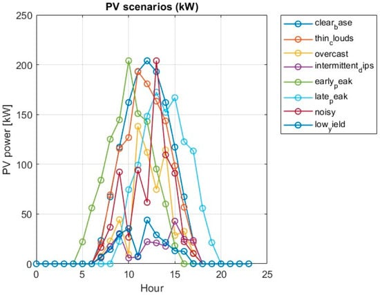
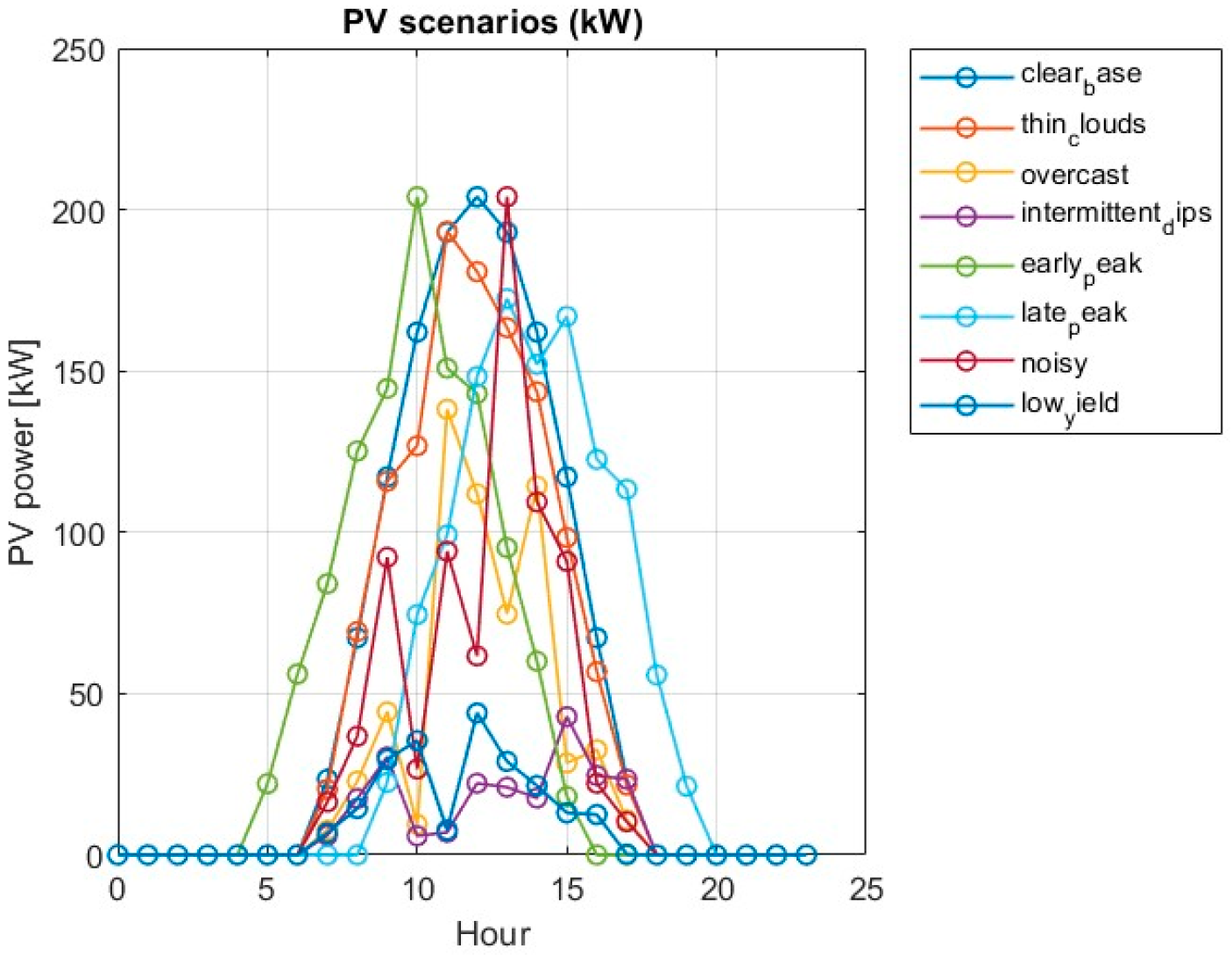
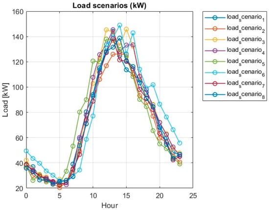
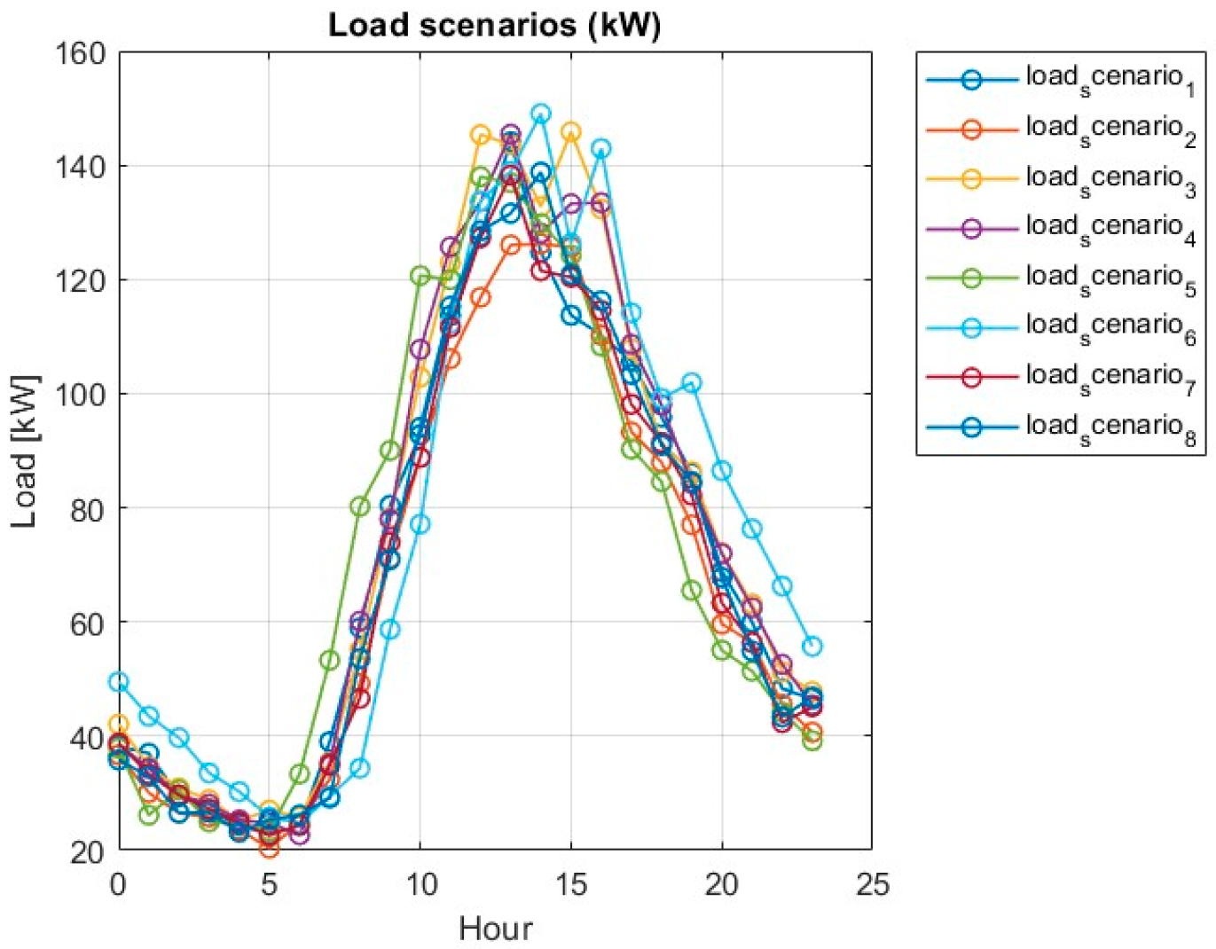
Eight representative 24 h scenarios are constructed from real measurements to capture a wide range of operating conditions, including stable, intermittent, noisy, and low-yield PV generation profiles. A representative measured day (4 February 2024) was used to verify that these profiles closely follow actual campus operation at hourly resolution. These scenarios are designed to test the generalization capability of the control strategies rather than to represent isolated operating days. Figure 5 and Figure 6 present the PV generation and load profiles for the eight scenarios.

Figure 5. The 8 PV power scenarios.

Figure 6. The 8 load scenarios.

3.2. Results from GA-Based Static Optimization

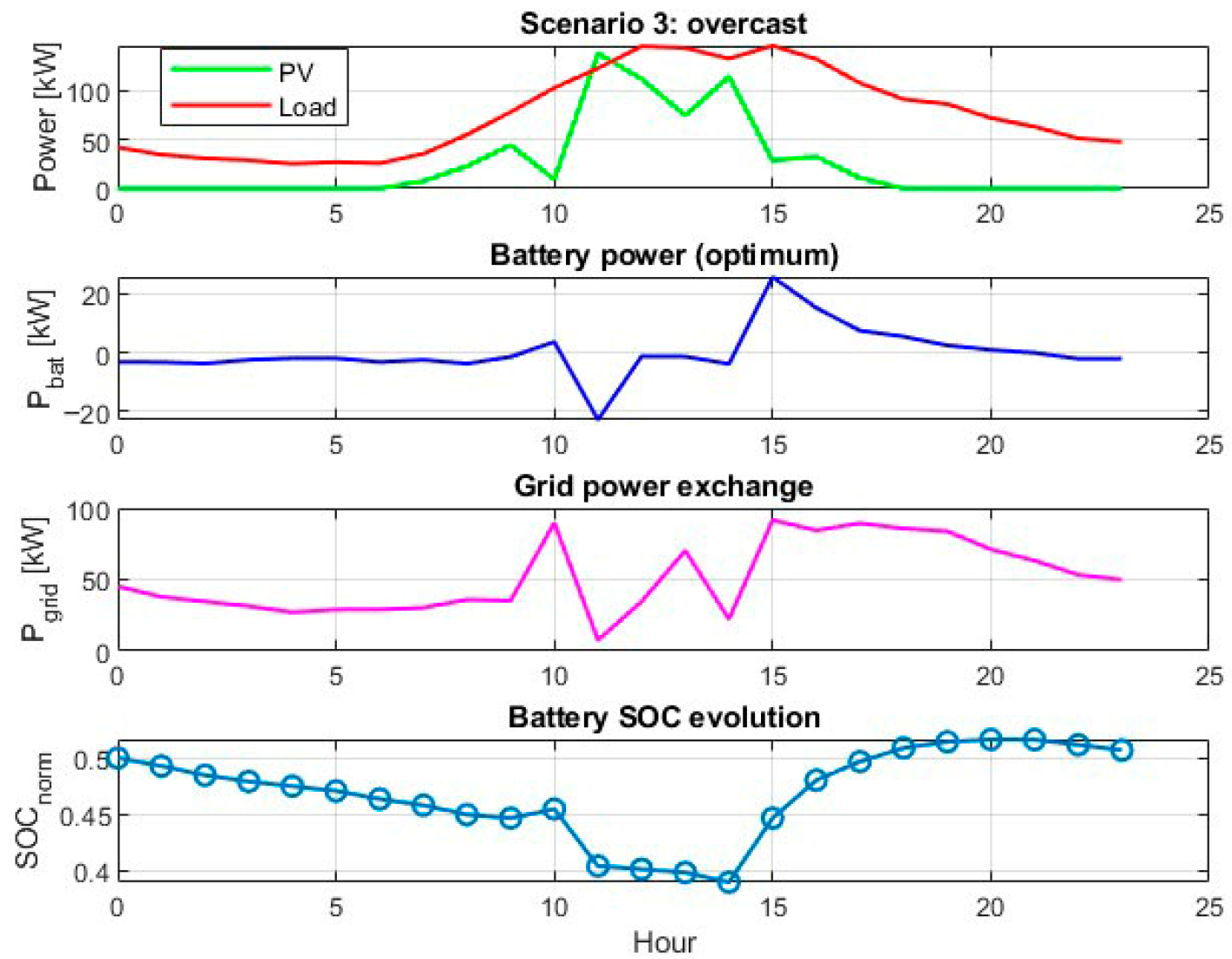
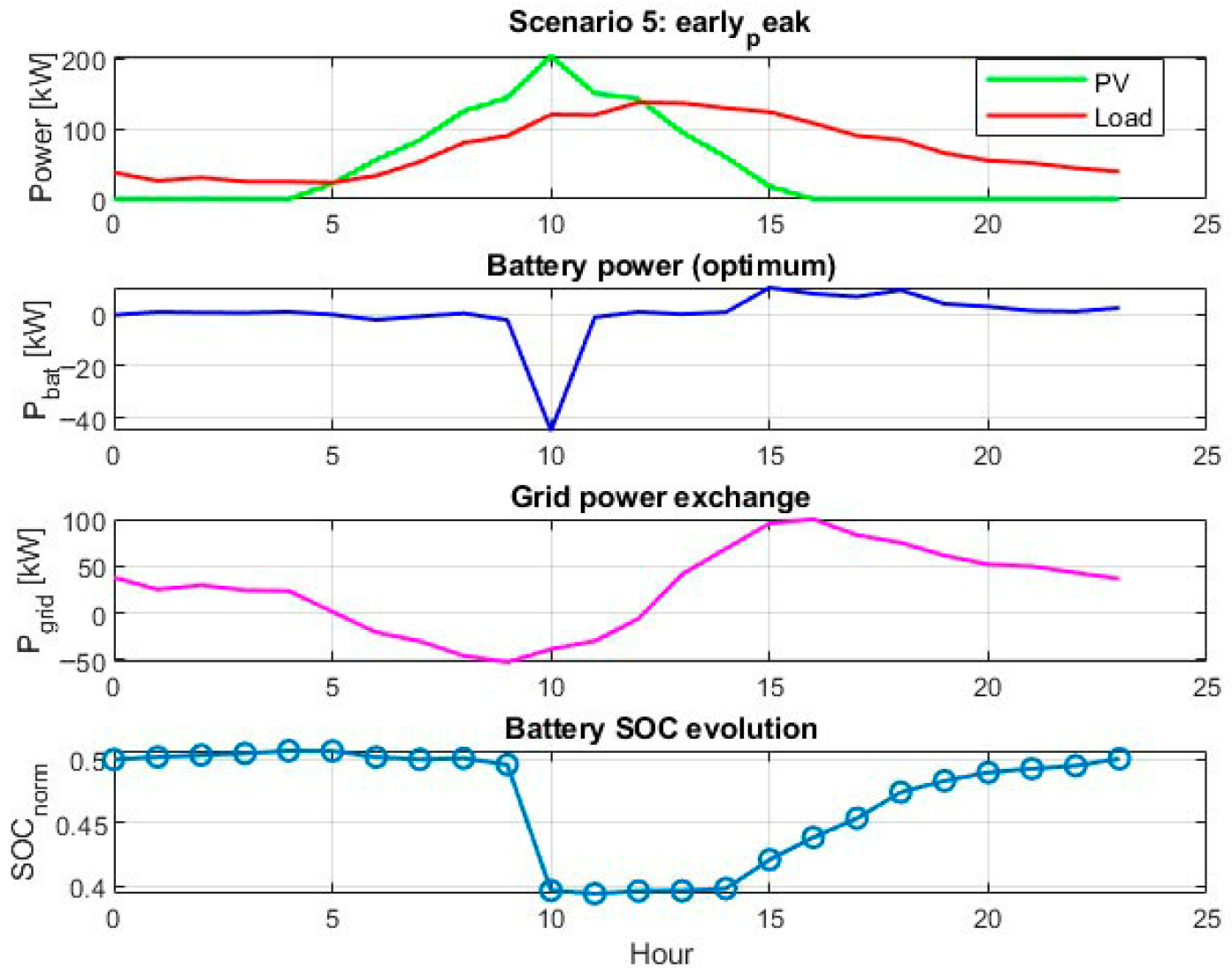
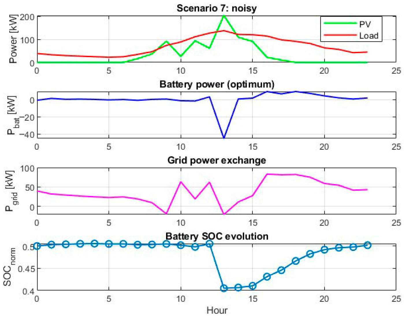
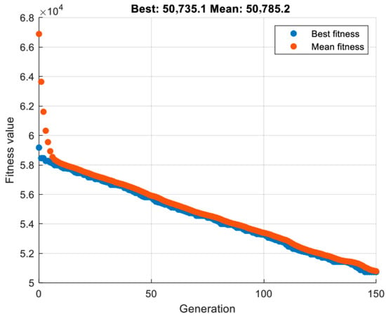
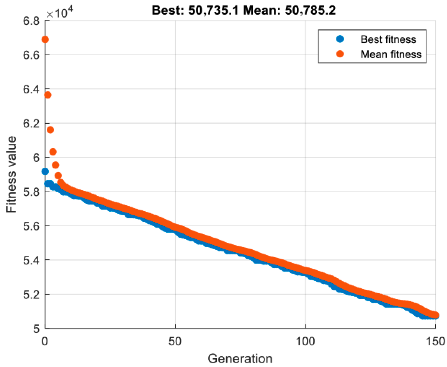
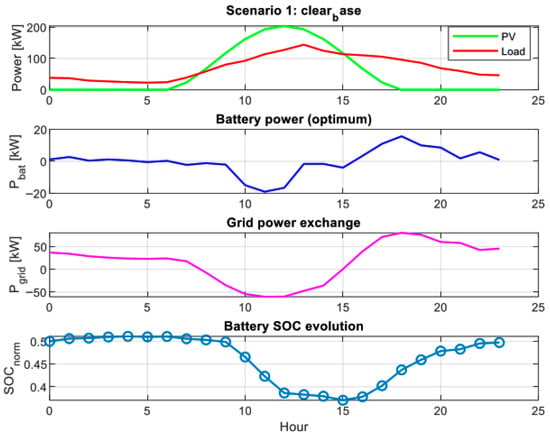
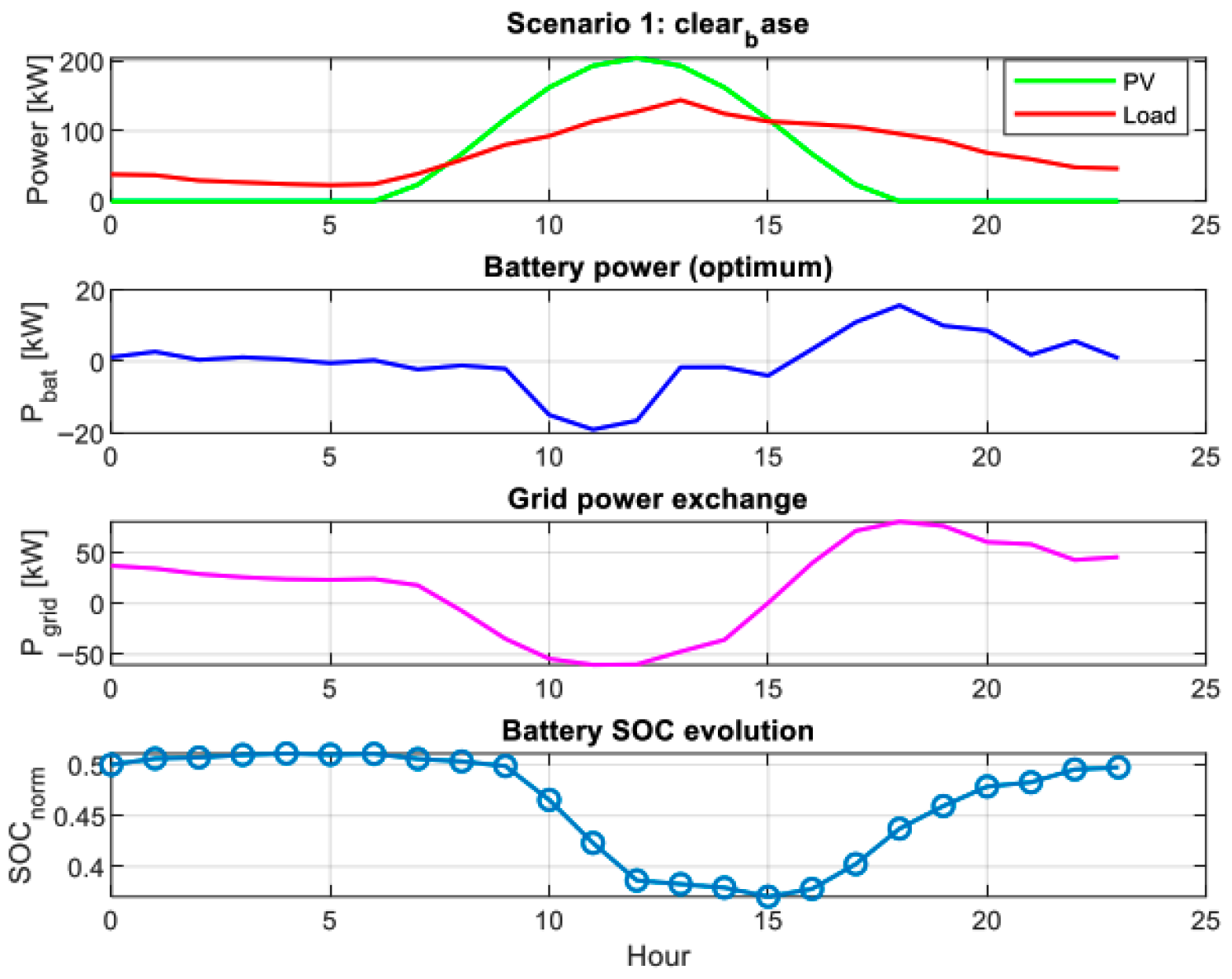
GA-based optimization is first applied to compute day-ahead reference schedules for all eight scenarios. Representative convergence and performance results for Scenario 1 (“clear_base”) are illustrated in Figure 7 and Figure 8. Similar convergence behavior is observed across all scenarios; therefore, only the resulting microgrid component trajectories are presented for the remaining cases (Figure 9, Figure 10, Figure 11, Figure 12, Figure 13, Figure 14, Figure 15 and Figure 16).

Figure 7. GA performance in Scenario 1.

Figure 8. Graphs for Scenario 1.

The results obtained for GA optimization in Scenario 2 and Scenario 3:

Figure 9. Graphs for Scenario 2.

Figure 9. Graphs for Scenario 2.

Figure 10. Graphs for Scenario 3.

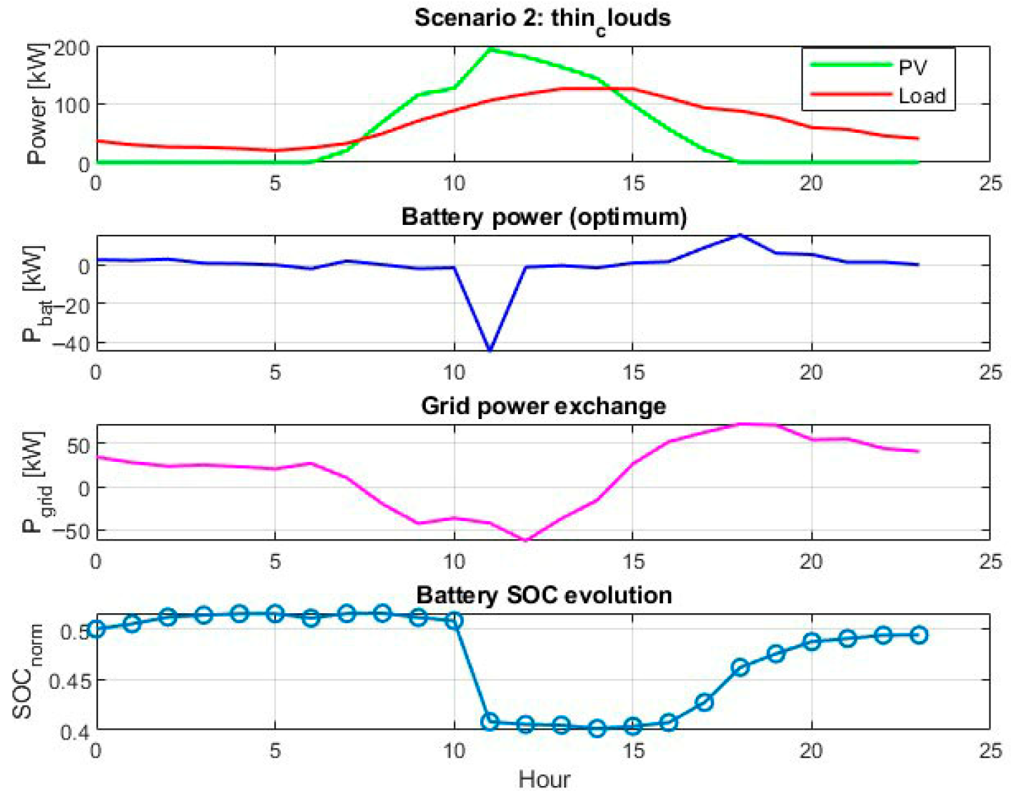
Figure 10. Graphs for Scenario 3.

The results obtained for GA optimization in Scenario 4 and Scenario 5:

Figure 11. Graphs for Scenario 4.

Figure 11. Graphs for Scenario 4.

Figure 12. Graphs for Scenario 5.

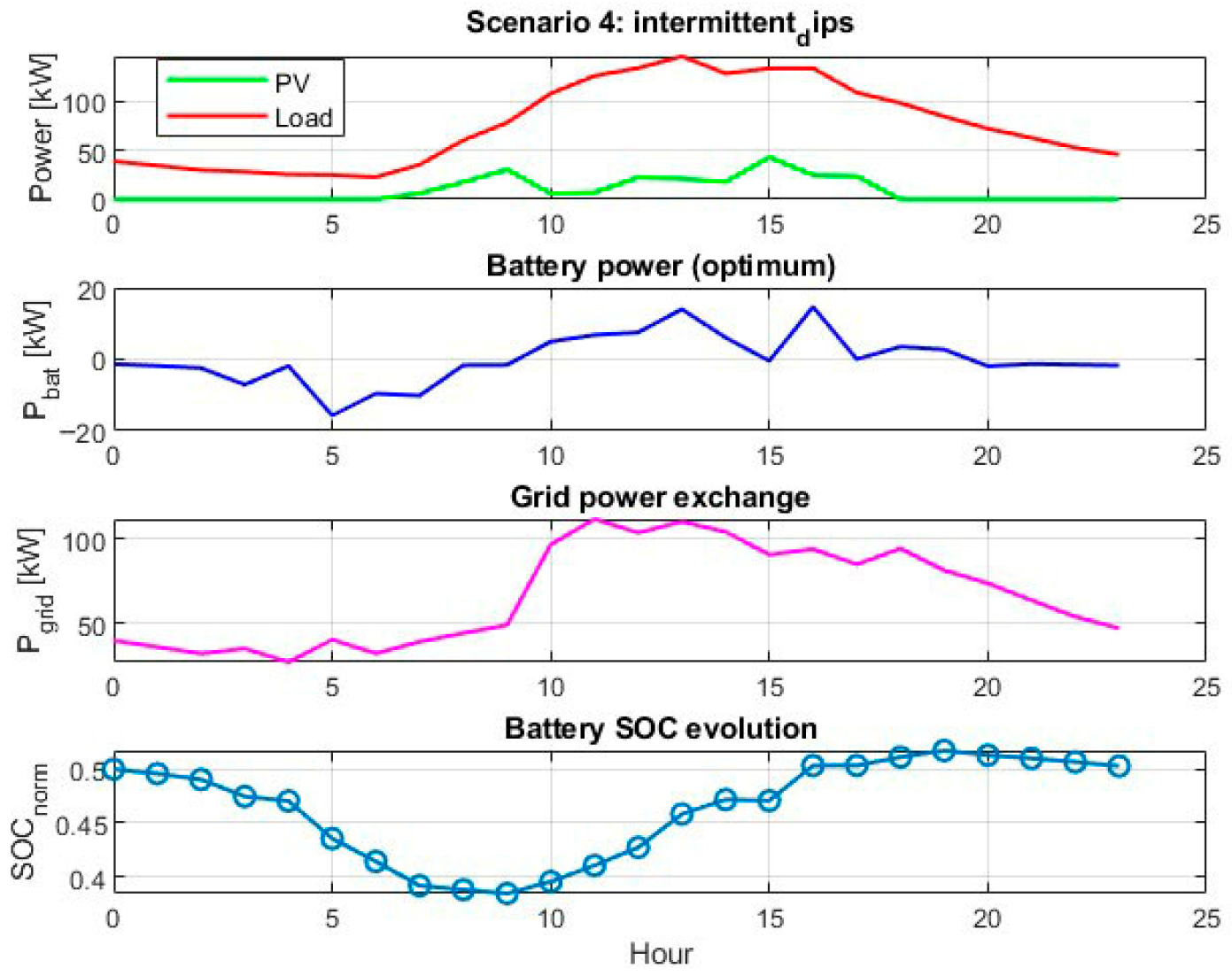
Figure 12. Graphs for Scenario 5.

The results obtained for GA optimization in Scenario 6 and Scenario 7:

Figure 13. Graphs for Scenario 6.

Figure 13. Graphs for Scenario 6.

Figure 14. Graphs for Scenario 7.

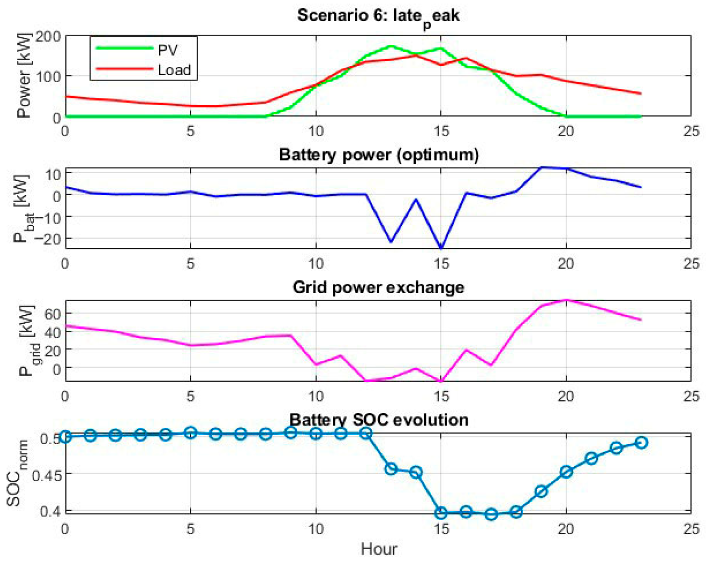
Figure 14. Graphs for Scenario 7.

The results obtained for GA optimization in Scenario 8 (“low_yield”):

Figure 15. GA performance in Scenario 8.

Figure 15. GA performance in Scenario 8.

Figure 16. Graphs for Scenario 8.

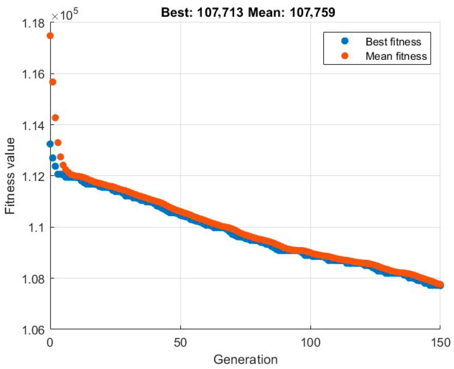
Figure 16. Graphs for Scenario 8.

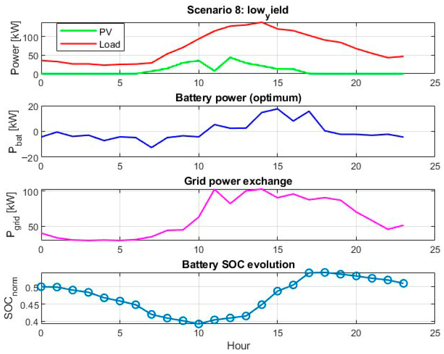
Across all scenarios, the GA yields feasible and stable operating points. Voltage constraints are fully respected, with zero time outside the predefined deadband in all cases. Energy exchange with the main grid and battery usage adapt consistently to the underlying PV and load conditions.

The quantitative results of GA optimization are summarized in Table 4 and Table 5. Scenarios with low or highly variable PV generation (overcast, intermittent_dips, and low_yield) exhibit higher grid energy imports and higher daily energy costs, whereas scenarios with stable and favorable PV generation (clear_base and thin_clouds) achieve lower costs. Battery throughput remains moderate in all scenarios, indicating that the optimization avoids unnecessary cycling.

Table 4. Results from GA optimization, part 1.

Scenario	Name	Pgrid_Mean_kW	Egrid_Pos_kWh	Egrid_Neg_kWh	Battery_ Throughput_kWh
1	“clear_base”	16.22	688.77	299.49	127.40
2	“thin_clouds”	17.126	666.92	255.89	110.78
3	“overcast”	51.39	1233.4	0.	126.81
4	“intermittent_dips”	66.202	1588.9	0.	127.96
5	“early_peak”	26.223	849.3	219.95	118.29
6	“late_peak”	29.212	744.33	43.245	113.04
7	“noisy”	37.195	931.97	39.29	107.21
8	“low_yield”	61.376	1473.	0.	120.27

Table 5. Results from GA optimization, part 2.

Scenario	Name	Voltage_ Frac_Outside	Voltage _Max_Abs_dV_pu	Voltage _Std_pu	JGA	Energy _Cost_USD
1	“clear_base”	0.	0.034277	0.017945	51,066.2956	68.422
2	“thin_clouds”	0.	0.030768	0.015615	42,130.6795	66.062
3	“overcast”	0.	0.035918	0.010297	79,125.0423	131.72
4	“intermittent_dips”	0.	0.046466	0.011876	124,669.9913	174.68
5	“early_peak”	0.	0.039037	0.017769	60,999.7378	90.963
6	“late_peak”	0.	0.027827	0.010297	36,298.2641	69.749
7	“noisy”	0.	0.033236	0.011507	6019.9	97.832
8	“low_yield”	0.	0.043204	0.011098	12,610.	161.86

3.3. Results from SAC Agent Training

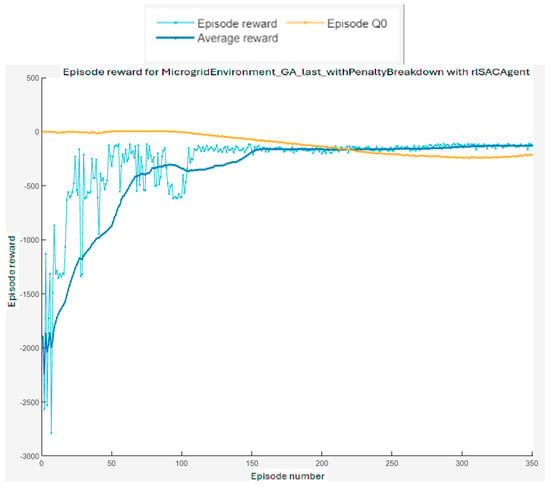
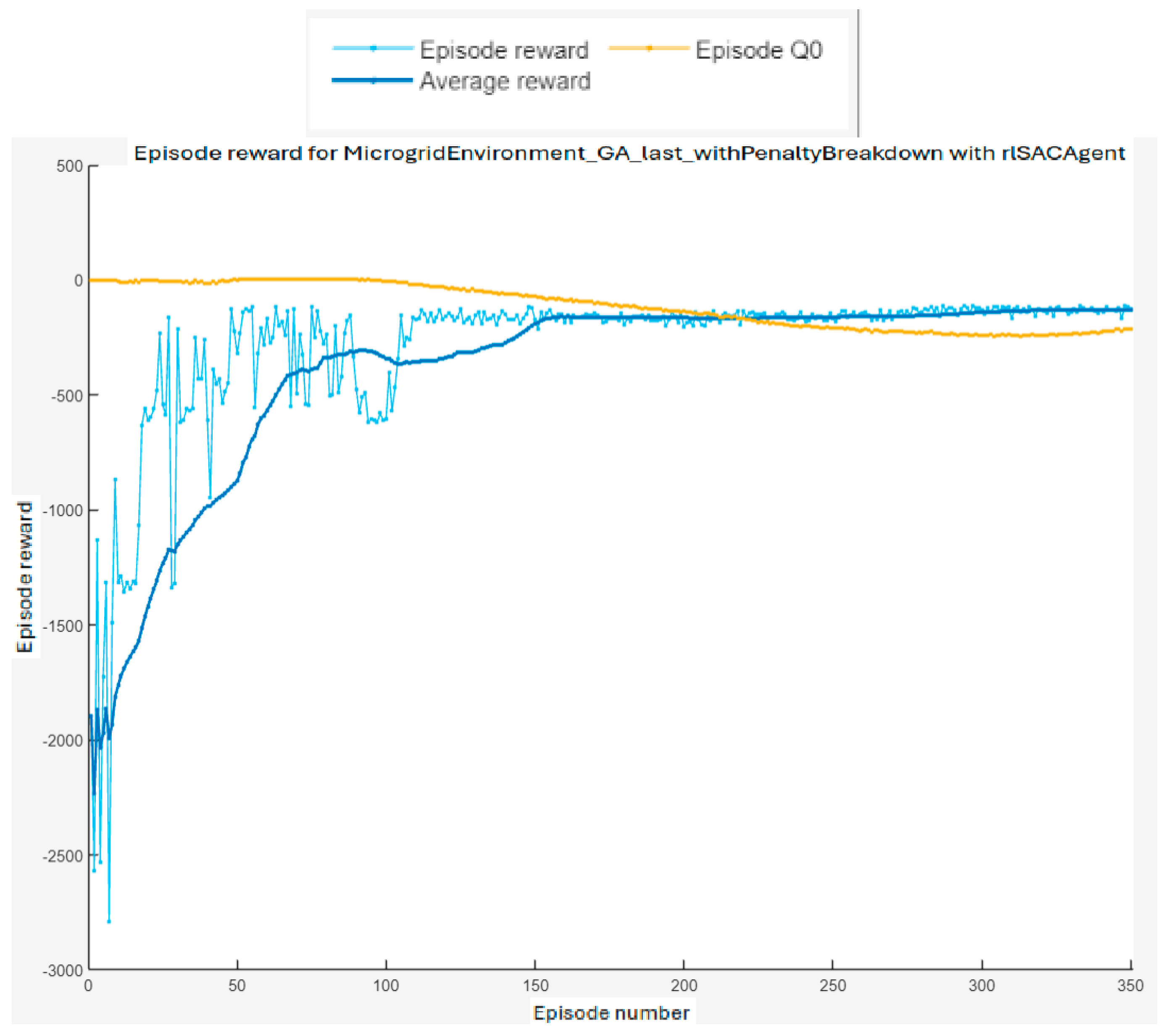
The SAC agent is trained separately for each scenario, with the objective of minimizing the aggregated reward function while respecting all operational constraints. Empirically, stable convergence is achieved within approximately 350 episodes for all scenarios. Figure 17 illustrates representative training dynamics for Scenario 1.

Figure 17. Agent training in Scenario 1.

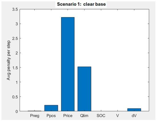
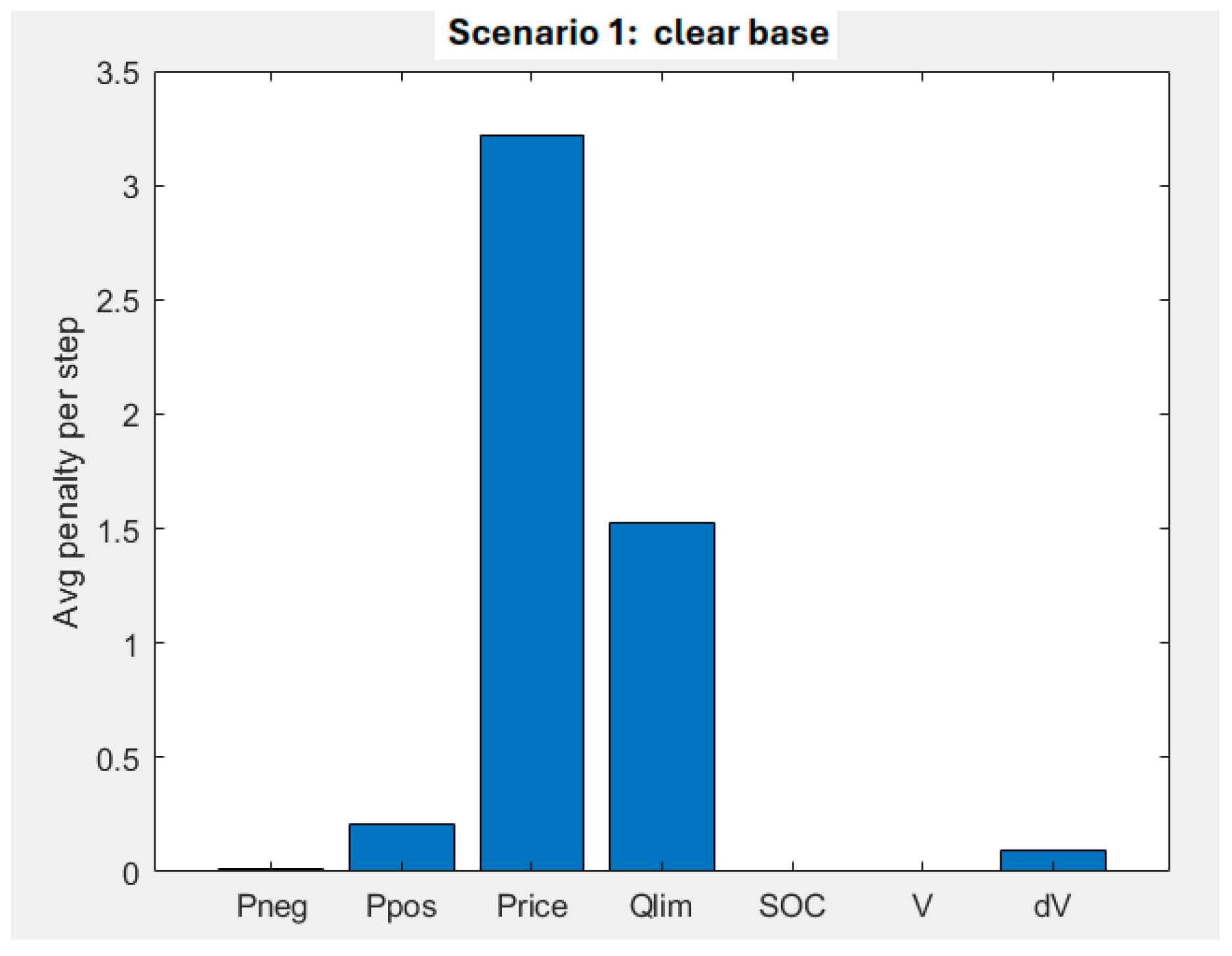
Differences between the critic’s estimated initial Q-value and the realized episode reward are expected due to policy stochasticity, entropy regularization, and terminal SOC penalties. Penalty breakdown analysis is used as an interpretability tool to assess the relative contribution of price, voltage, and SOC-related terms. A representative example for Scenario 1 is shown in Figure 18.

Figure 18. Penalty breakdown chart for Scenario 1.

The final training results are summarized in Table 6. Average episode rewards lie within a relatively narrow range across scenarios, indicating consistent learning behavior under diverse operating conditions.

Table 6. Results for SAC agent training across 8 scenarios.

Scenario No.	Scenario Name	Average Reward	Final Reward
1	“Clear base”	−5.0879	−4.1537
2	“Thin clouds”	−6.5381	−2.992
3	“Overcast”	−9.5969	−4.0345
4	“Intermittent dips”	−7.9941	−3.3311
5	“Early peak”	−10.014	−4.3793
6	“Late peak”	−14.448	−3.9954
7	“Noisy”	−9.1458	−24.857
8	“Low yield”	−7.5129	−8.7054

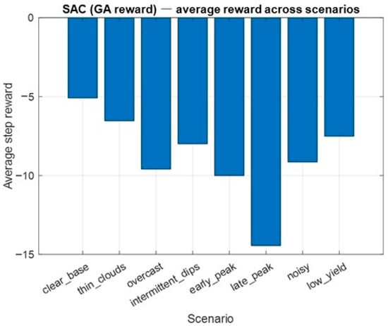
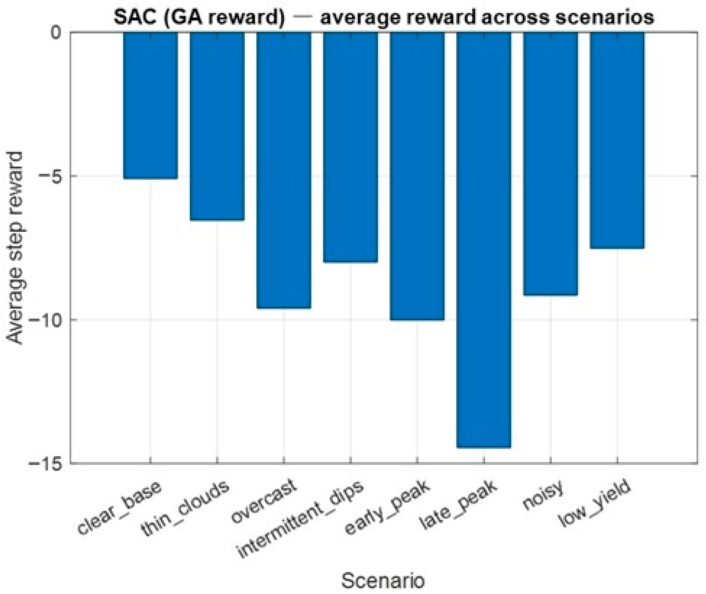
The average reward values for all scenarios are presented in Figure 19.

Figure 19. Average reward across scenarios.

3.4. Convergence and Reward Statistics

Across all eight scenarios, the SAC agent demonstrates stable convergence and consistent learning dynamics. Scenarios with stable and favorable PV generation yield relatively mild penalties, whereas scenarios with a low or highly variable PV output incur higher penalties due to increased grid energy purchases and voltage-smoothing requirements.

The “Noisy” scenario exhibits a notably lower final reward compared to other cases. This behavior is attributed to the highly stochastic nature of the PV and load profiles, which increases voltage- and SOC-related penalties. Importantly, reward values are scenario-dependent and reflect trade-offs between economic performance and constraint enforcement rather than direct measures of energy efficiency.

3.5. GA-RL Comparison Using RMSE Metrics

To quantify the difference between static scheduling and adaptive control, RMSE metrics are evaluated for battery state-of-charge (SOC) trajectories and grid power exchange. RMSE_SOC and RMSE_Pgrid are defined in (29) and (30), respectively.

• RMSE for SOC

T is the number of time steps (e.g., 24 for 24 h);

SOC^GA(t_i) is the normalized state of charge from the GA model at time t_i;

SOC^RL(t_i) is the normalized state of charge from the RL simulation at time t_i.

RMSE for the SOC is calculated as follows:

$${RMSE}_{SOC} = \sqrt{{\displaystyle \frac{1}{T}}{\sum }_{i=1}^T{\left({SOC}^{GA}(t_i)-{SOC}^{RL}(t_i)\right)}^2}$$

(29)

When RMSE_SOC = 0, the GA and RL match completely. When RMSE_SOC = 1, there is complete divergence (maximum possible, since SOC is normalized in [0, 1]).

• RMSE for active power to the grid

Similarly, if the following holds:

$P_{grid}^{GA}(t_i)$ is the active power to/from the grid in GA optimization [kW];

$P_{grid}^{RL}(t_i)$ is the same amount of power obtained from the RL agent;

T is the number of steps.

Then, we obtain the following:

$${RMSE}_{Pgrid} = \sqrt{{\displaystyle \frac{1}{T}}{\sum }_{i=1}^T{\left(P_{grid}^{GA}(t_i)-P_{grid}^{RL}(t_i)\right)}^2}$$

(30)

These metrics are diagnostic rather than performance indicators, as the GA and SAC optimize fundamentally different objectives. The GA targets balanced day-ahead energy flows, whereas the SAC agent optimizes an aggregated economic and operational reward.

The RMSE results for all scenarios are presented in Table 7.

Table 7. Operational KPIs for GA-based scheduling and SAC-based control across 8 scenarios.

Scenario Index	Scenario Name	RMSESOC	RMSEPgrid [kW]
1	“Clear base”	0.3118	24.313
2	“Thin clouds”	0.30041	23.204
3	“Overcast”	0.42972	32.631
4	“Intermittent dips”	0.42842	28.825
5	“Early peak”	0.31498	27.481
6	“Late peak”	0.37009	25.746
7	“Noisy”	0.42808	25.866
8	“Low yield”	0.43595	29.686

The data of the PV system energy generation and the load (energy consumption) of the microgrid for all 8 scenarios are available and are presented in Table 8 and Table 9:

Table 8. Data on PV system energy generation [kW] across 8 scenarios (24 h, 1 h steps).

Scen. 1	Scen. 2	Scen. 3	Scen. 4	Scen. 5	Scen. 6	Scen. 7	Scen. 8
0	0	0	0	0	0	0	0
0	0	0	0	0	0	0	0
0	0	0	0	0	0	0	0
0	0	0	0	0	0	0	0
0	0	0	0	0	0	0	0
0	0	0	0	22.074	0	0	0
0	0	0	0	56.090	0	0	0
23.465	20.347	7.695	6.086	84.068	0	16.427	6.852
67.295	69.241	22.858	17.453	125.208	0	36.783	14.409
117.167	115.817	44.357	30.388	144.575	22.475	92.243	29.614
162.061	126.814	9.457	5.894	204.0	74.485	26.630	35.420
192.992	193.329	138.136	7.019	150.904	99.199	94.105	7.715
204.0	180.799	111.951	22.194	142.968	148.284	61.689	44.007
192.992	163.435	74.642	20.997	95.261	172.419	204.0	28.994
162.061	143.544	114.342	17.632	60.062	152.053	109.417	21.472
117.167	98.391	28.504	42.838	18.090	166.916	91.002	13.033
67.295	56.783	32.615	24.604	5.131 × 10−24	122.587	22.196	12.515
23.465	21.693	10.883	23.465	0	113.328	10.276	0.227
7.087 × 10−24	6.523 × 10−24	3.883 × 10−24	7.087 × 10−24	0	55.785	3.358 × 10−24	2.592 × 10−24
0	0	0	0	0	21.307	0	0
0	0	0	0	0	6.069 × 10−24	0	0
0	0	0	0	0	0	0	0
0	0	0	0	0	0	0	0
0	0	0	0	0	0	0	0

Table 9. Data on microgrid energy consumption [kW] across 8 scenarios (24 h, 1 h steps).

Scen. 1	Scen. 2	Scen. 3	Scen. 4	Scen. 5	Scen. 6	Scen. 7	Scen. 8
38.186	36.732	42.089	38.601	37.858	49.504	38.779	35.819
36.992	30.092	34.641	34.321	26.141	43.482	33.353	32.925
29.366	26.485	30.906	29.737	30.569	39.729	29.620	26.543
26.904	25.835	28.870	28.091	24.971	33.540	27.260	26.651
24.387	23.613	25.275	25.322	24.753	30.272	24.768	23.153
22.753	20.345	27.024	24.721	23.414	25.786	22.606	25.358
24.299	24.816	25.822	22.711	33.365	24.805	24.471	26.183
39.027	32.463	35.473	35.205	53.274	29.432	34.858	29.185
58.958	49.215	55.092	60.134	80.242	34.378	46.612	53.561
80.419	71.129	78.213	77.959	90.024	58.687	73.939	70.897
92.778	88.810	102.866	107.745	120.652	77.139	88.793	94.067
113.660	106.112	122.929	125.691	119.951	112.285	111.603	115.278
127.565	116.858	145.354	133.627	137.972	133.724	127.259	128.497
144.086	126.025	143.600	145.430	136.931	138.892	138.223	131.573
124.750	126.219	132.756	128.093	129.783	149.037	121.506	138.768
113.708	125.635	145.849	133.255	124.253	126.296	120.358	120.888
110.193	110.260	132.332	133.434	108.326	142.919	114.559	116.211
105.684	93.288	107.805	108.618	90.278	114.147	98.104	103.371
95.891	87.964	91.240	97.995	85.566	99.167	91.435	90.903
86.051	77.018	86.322	84.286	65.512	101.897	82.205	84.557
68.849	59.615	72.138	71.946	55.041	86.502	63.285	67.775
59.946	56.429	63.179	62.481	51.384	76.322	56.387	54.928
48.322	45.583	51.254	52.567	44.202	66.270	42.354	43.340
46.471	40.677	47.775	45.459	39.183	55.708	45.111	46.861

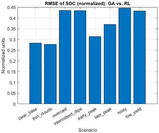
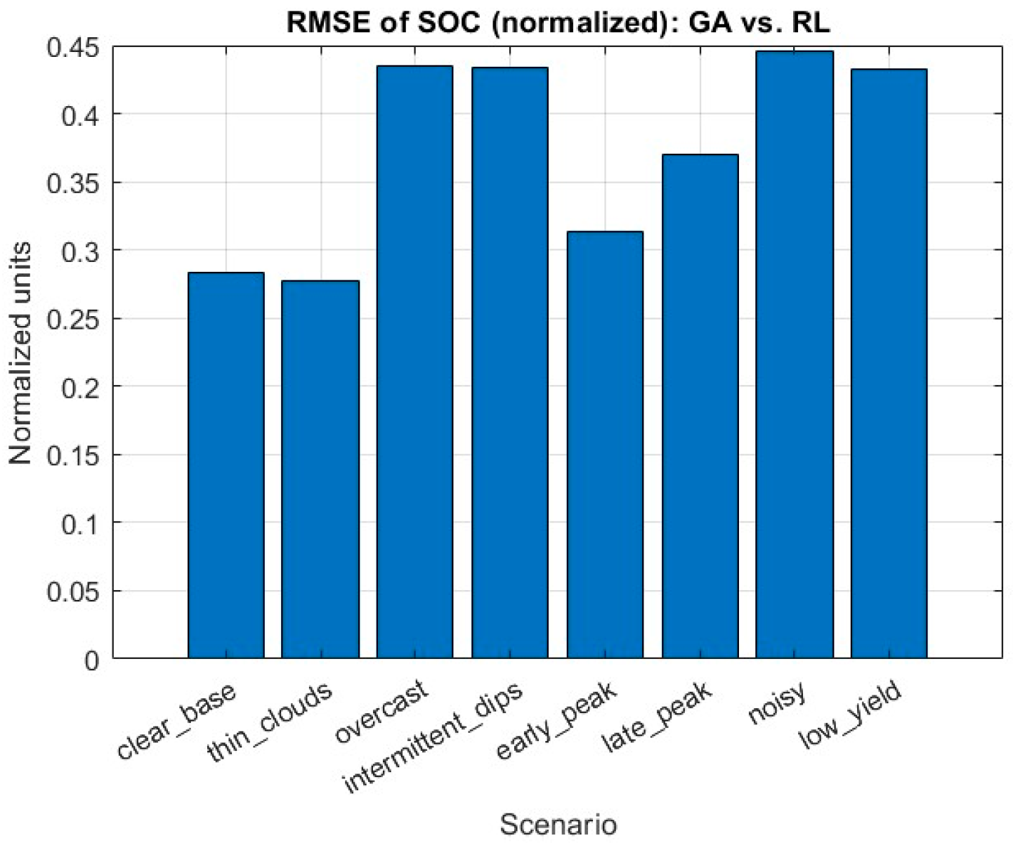
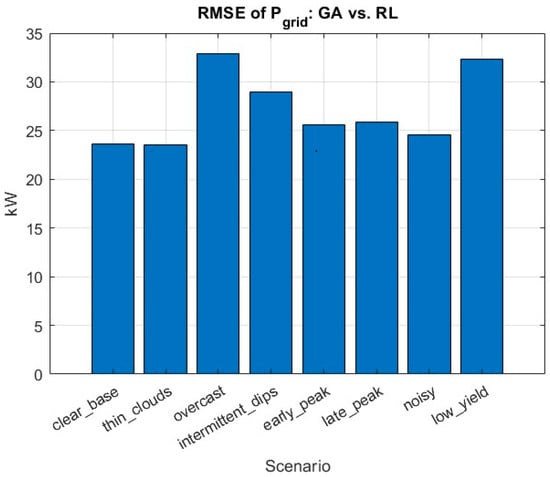
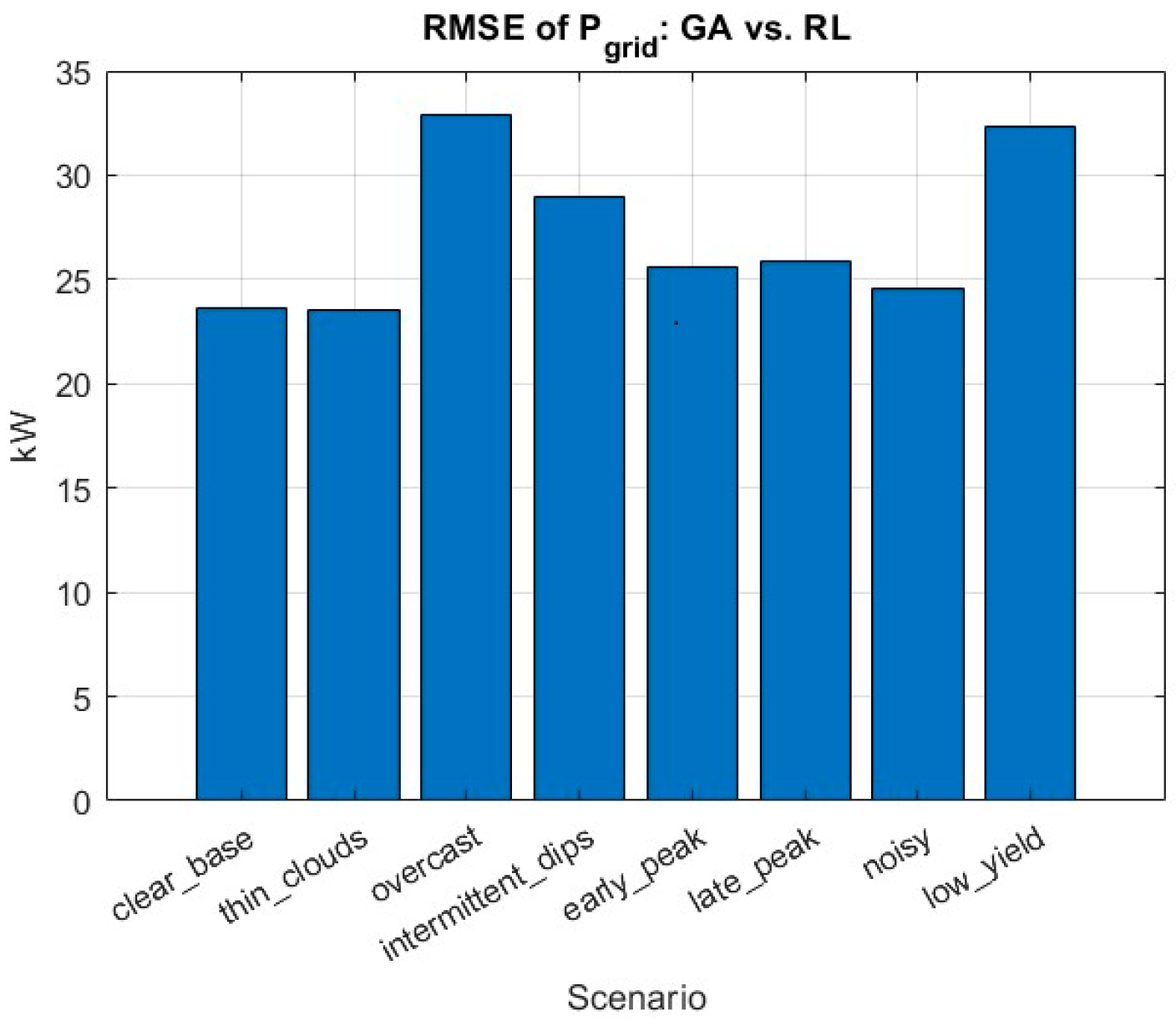
These results are illustrated in Figure 20 and Figure 21. Higher RMSE values are observed under adverse generation conditions, where the SAC agent deliberately deviates from the GA reference by charging earlier during low-tariff periods. Despite larger deviations, all operational constraints remain satisfied.

Figure 20. RMSE_SOC for all scenarios.

Figure 21. RMSE_Pgrid for all scenarios.

4. Discussion

Static GA-based optimization and the SAC-based controller play complementary roles within the proposed two-stage energy management framework. As shown in Table 4 and Table 5, the GA provides stable day-ahead reference schedules that strictly satisfy voltage constraints and yield interpretable operating points across all scenarios. In contrast, the SAC-based controller adapts these references online, responding to deviations from forecasted conditions without re-solving the optimization problem. The RMSE results in Table 7 confirm that the SAC agent does not attempt to replicate the GA trajectories but instead converges to economically rational policies that prioritize cost reduction while respecting all operational constraints.

The scenario-dependent behavior of the SAC agent is clearly reflected in the reward statistics summarized in Table 6 and Figure 19. Scenarios with stable and favorable PV generation achieve relatively mild penalties, whereas highly variable or low-yield scenarios result in lower rewards due to increased grid reliance and stronger voltage- and SOC-related penalties. Notably, the “Noisy” scenario exhibits a significantly lower final reward despite not representing the worst operational performance according to system-level KPIs (Table 7). This confirms that reward values are scenario-dependent and should be interpreted as indicators of constraint trade-offs rather than direct measures of energy efficiency.

The RMSE-based comparison further clarifies the functional distinction between static and adaptive control. Higher RMSE values are observed under adverse PV conditions, where the SAC agent deliberately charges the battery earlier during low-tariff periods to hedge against expensive future imports. Although this behavior increases the deviation from the GA reference, it leads to economically superior operation while maintaining voltage stability and SOC limits. Consequently, RMSE metrics serve as diagnostic indicators of policy divergence rather than control error.

The proposed framework targets the operational priorities of campus microgrids, namely, reducing the grid dependency and maximizing local PV self-consumption. Explicit modeling of energy export and market participation is not included, as these depend on region-specific regulatory and tariff structures. However, the results demonstrate that both the GA objective function and the SAC reward formulation can be naturally extended with export-related terms if market participation is required.

Although the evaluation is conducted in a simulation environment, it relies on measured PV generation and campus load data, and the controller operates at an hourly supervisory level. This makes the framework compatible with standard PLC or industrial PC platforms. Required measurements and control signals are readily available in modern microgrid architectures, enabling practical deployment without additional sensing infrastructure.

Battery degradation [28] and cycling costs are not explicitly modeled, as the study focuses on short-term operational management at daily time scales. The moderate battery throughput observed across all scenarios (Table 4) suggests that excessive cycling is avoided. Nevertheless, cycle-based or state-of-health-dependent degradation terms can be readily incorporated into both the GA objective and the SAC reward in future extensions.

Regarding scalability, the computational burden is dominated by the offline optimization and training phases. While GA complexity increases with problem size, it does not affect real-time operation. Online execution of the SAC-based EMS involves only lightweight NN inference, resulting in negligible runtime overhead. For larger systems, scalability can be addressed through state aggregation, hierarchical control, or multi-agent extensions, which are well-established approaches in smart campus and smart city applications.

Validity of PCC Voltage Approximation

The PCC voltage model is based on a linear Thévenin/LinDistFlow-type approximation, which is appropriate for supervisory energy management studies where voltage deviations remain moderate. As confirmed by the GA and SAC results, voltage remains within the prescribed deadband in all scenarios (Table 5 and Table 7). Bounded actions and constraint-related penalties discourage operation in regimes where linearization accuracy would degrade. While extreme operating points could reduce model fidelity, such conditions are outside the targeted EMS operating envelope and are effectively avoided by the proposed control framework.

5. Conclusions

This paper presents an integrated GA-SAC framework for supervisory energy management of a microgrid with high penetration of PV generation and battery energy storage. The proposed approach combines offline static optimization using the GA with adaptive real-time control based on a soft actor-critic RL agent, addressing both economic efficiency and operational constraints under uncertainty.

Overall, the proposed GA-SAC framework demonstrates that RL can serve as an effective adaptive supervisory controller for microgrids, complementing traditional optimization by responding to deviations from forecasted operation without re-solving complex optimization problems. The framework is computationally efficient for real-time deployment and scalable to larger campus or district-level systems, making it a promising foundation for future intelligent energy management applications.

Limitations and Future Research Directions

While the proposed framework shows strong performance in simulation, several limitations should be acknowledged. The evaluation does not explicitly address real-time deployment issues such as communication delays, hardware-in-the-loop validation, controller execution on industrial EMS platforms, and cyber security aspects.

The focus of this work is on short-term operational energy management and self-consumption optimization. Long-term planning aspects such as battery degradation, emissions minimization, demand response participation, and market-based energy trading are not explicitly modeled, but the GA-SAC framework can be extended to multi-objective optimization models.

References

- Ahmad, S.; Shafiullah, M.; Ahmed, C.B.; Alowaifeer, M. A Review of Microgrid Energy Management and Control Strategies. IEEE Access 2023, 11, 21729–21757. [Google Scholar] [CrossRef] [Scilit]
- Gao, K.; Wang, T.; Han, C.; Xie, J.; Ma, Y.; Peng, R. A Review of Optimization of Microgrid Operation. Energies 2021, 14, 2842. [Google Scholar] [CrossRef] [Scilit]
- Eyimaya, S.E.; Altin, N. Review of Energy Management Systems in Microgrids. Appl. Sci. 2024, 14, 1249. [Google Scholar] [CrossRef] [Scilit]
- Esparza, A.; Blondin, M.; Trovão, J.P.F. A Review of Optimization Strategies for Energy Management in Microgrids. Energies 2025, 18, 3245. [Google Scholar] [CrossRef] [Scilit]
- Goldberg, D.E. Genetic Algorithms in Search, Optimization and Machine Learning; Addison Wesley: Reading, MA, USA, 1989; 432p. [Google Scholar]
- Trivedi, R.; Khadem, S. Implementation of artificial intelligence techniques in microgrid control environment: Current progress and future scopes. Energy AI 2022, 8, 100147. [Google Scholar] [CrossRef] [Scilit]
- Gupta, Y.; Amin, M. A Neural Network-Based Energy Management System for PV-Battery Based Microgrids. arXiv 2022. [Google Scholar] [CrossRef] [Scilit]
- Sutton, R.S.; Barto, A.G. Reinforcement Learning: An Introduction, 2nd ed.; The MIT Press: Cambridge, MA, USA; London, UK, 2014, 2015; Available online: https://web.stanford.edu/class/psych209/Readings/SuttonBartoIPRLBook2ndEd.pdf (accessed on 1 November 2025).
- She, B.; Li, F.; Cui, H.; Zhang, J.; Bo, R. Fusion of Microgrid Control with Model-free Reinforcement Learning: Review and Vision. IEEE Trans. Smart Grid 2022, 14, 3232–3245. [Google Scholar] [CrossRef] [Scilit]
- Hu, C.; Cai, Z.; Zhang, Y.; Yan, R.; Cai, Y.; Cen, B. A soft actor-critic deep reinforcement learning method for multi-timescale coordinated operation of microgrids. Prot. Control. Mod. Power Syst. 2022, 7, 29. [Google Scholar] [CrossRef] [Scilit]
- Bhujel, N.; Rai, A.; Tamrakar, U.; Zhu, Y.; Hansen, T.M.; Hummels, D.; Tonkoski, R. Soft Actor-Critic Based Voltage Support for Microgrid Using Energy Storage Systems. SAND2023-07664C. 2023. Available online: https://www.osti.gov/servlets/purl/2431100 (accessed on 3 November 2025).
- Shen, H.; Shen, X.; Chen, Y. Real-Time Microgrid Energy Scheduling Using Meta-Reinforcement Learning. Energies 2024, 17, 2367. [Google Scholar] [CrossRef] [Scilit]
- Khanghah, M.S.; Moghaddam, F.; Suratgar, A.; Menhaj, M.B. SAC-Based Distributed Optimal Control of Generation Cost in DC Microgrids. In Proceedings of the 2025 IEEE Seventh International Conference on DC Microgrids (ICDCM), Tallinn, Estonia, 4–6 June 2025; pp. 1–7. [Google Scholar] [CrossRef] [Scilit]
- Sharma, D.D.; Bansal, R.C. LSTM-SAC reinforcement learning based resilient energy trading for networked microgrid system. AIMS Electron. Electr. Eng. 2025, 9, 165–191. [Google Scholar] [CrossRef] [Scilit]
- Du, W.; Huang, X.; Zhu, Y.; Wang, L.; Deng, W. Deep reinforcement learning for adaptive frequency control of island microgrid considering control performance and economy. Front. Energy Res. 2024, 12, 1361869. [Google Scholar] [CrossRef] [Scilit]
- Wang, Y.; Cui, Y.; Li, Y.; Xu, Y. Collaborative optimization of multi-microgrids system with shared energy storage based on multi-agent stochastic game and reinforcement learning. Energy 2023, 280, 128182. [Google Scholar] [CrossRef] [Scilit]
- Gao, J.; Li, Y.; Wang, B.; Wu, H. Multi-Microgrid Collaborative Optimization Scheduling Using an Improved Multi-Agent Soft Actor-Critic Algorithm. Energies 2023, 16, 3248. [Google Scholar] [CrossRef] [Scilit]
- CHSM72M-HC 450 Solar Panel from Astronergy: Specs, Prices and Reviews. solarreviews.com. Available online: https://amonraenergy.eu/produkt/astronergy-astro-4-semi-chsm72m-hc-450w (accessed on 30 October 2025).
- Borni, A.; Abdelkirim, T.; Bouarroudj, N.; Bouchakour, A.; Zaghba, L.; Lakhdari, A.; Zarour, L. Optimized MPPT Controllers Using GA for Grid Connected Photovoltaic Systems, Comparative study. Energy Procedia 2017, 119, 278–296. [Google Scholar] [CrossRef] [Scilit]
- Albarakati, A.J.; Boujoudar, Y.; Azeroual, M.; Jabeur, R.; Aljarbouh, A.; El Moussaoui, H.; Lamhamdi, T.; Ouaaline, N. Real-Time Energy Management for DC Microgrids Using Artificial Intelligence. Energies 2021, 14, 5307. [Google Scholar] [CrossRef] [Scilit]
- Leyva, R.; Alonso, C.; Queinnec, I.; Cid-Pastor, A.; Lagrange, D.; Martinez-Salamero, L. MPPT of Photovoltaic Systems Using Extremum—Seeking Control. IEEE Trans. Aerosp. Electron. Syst. 2006, 42, 249–258. [Google Scholar] [CrossRef] [Scilit]
- Boshnjaku, E.; Qehaja, B.; Hajrizi, E.; Guliashki, V.; Marinova, G. A Web-Based Hybrid Optimization Platform for Real-Time Microgrid Energy Management. In Proceedings of the ConTEL Symposium Within the 33rd International Conference on Software, Telecommunications and Computer Networks (SoftCOM 2025), Split, Croatia, 18–20 September 2025; Available online: https://2025.softcom.fesb.unist.hr/wp-content/uploads/2025/09/FINAL_PROGRAM_2025.pdf (accessed on 10 September 2025).
- Meng, Q.; Hussain, S.; Luo, F.; Wang, Z.; Jin, X. An Online Reinforcement Learning-Based Energy Management Strategy for Microgrids with Centralized Control. IEEE Trans. Ind. Appl. 2025, 61, 1501–1510. [Google Scholar] [CrossRef] [Scilit]
- Grib, M.; Sirbu, I.-G.; Mandache, L.; Stanculescu, M.; Iordache, M.; Bobaru, L.; Niculae, D. Generation Algorithms for Thévenin and Norton Equivalent Circuits. Energies 2025, 18, 1344. [Google Scholar] [CrossRef] [Scilit]
- Moffat, K.; von Meier, A. Linear quadratic phasor control of unbalanced distribution networks. In Proceedings of the 2021 IEEE Madrid PowerTech, Madrid, Spain, 28 June–2 June 2021; IEEE: New York, NY, USA, 2021; pp. 1–6. [Google Scholar]
- Nazir, R.; Laksono, H.D.; Waldi, E.P.; Ekaputra, E.; Coveria, P. Renewable Energy Sources Optimization: A Micro-Grid Model Design. Energy Procedia 2014, 52, 316–327. [Google Scholar] [CrossRef] [Scilit]
- ENTSO-E. Network Codes Home. Available online: https://www.entsoe.eu/network_codes/ (accessed on 5 November 2025).
- Meng, Q.; He, Y.; Hussain, S.; Lu, J.; Guerrero, J.M. Design and optimization of solar photovoltaic microgrids with adaptive storage control for residential standalone systems. Energy Rep. 2025, 14, 989–997. [Google Scholar] [CrossRef] [Scilit]
Disclaimer/Publisher’s Note: The statements, opinions and data contained in all publications are solely those of the individual author(s) and contributor(s) and not of MDPI and/or the editor(s). MDPI and/or the editor(s) disclaim responsibility for any injury to people or property resulting from any ideas, methods, instructions or products referred to in the content. |
© 2026 by the authors. Licensee MDPI, Basel, Switzerland. This article is an open access article distributed under the terms and conditions of the Creative Commons Attribution (CC BY) license.