An InterpreTable Fuzzy-Logic Framework for Diagnosis and Fault-Signature Analysis of Operational, Corrosion, Structural, and Metallurgical Failure Scenarios in an Aged Pipeline Network

Abstract

Aged pipeline networks face interacting operational, electrochemical, structural, and metallurgical degradation mechanisms that are often assessed independently, limiting diagnosis of system-wide failure propagation. This study develops an integrated, interpreTable fuzzy-logic framework to detect, quantify, and isolate failure scenarios in a 572 km pipeline network. The methodology combines 596 historical SCADA and SAP records, cathodic-protection and soil measurements from 907 evaluation points, 4651 ultrasonic-inspection anomalies, mechanical and metallographic characterization of API L X65 steel, and validated expert knowledge. Four Mamdani fuzzy inference systems were constructed to represent operational capacity, cathodic-protection performance, mechanical integrity, and metallurgical degradation. Their outputs were combined into a unified fault-signature matrix comprising 28 failure scenarios. Scenario FS-3 produced the broadest systemic response by activating all diagnostic residuals. Metallurgical scenarios FS-22 to FS-28 activated 61% of the matrix, showing their extensive influence on pipeline integrity. Structural scenarios FS-15 to FS-21 showed progressively broader signatures as wall deterioration increased. Meanwhile, FS-1, FS-2, FS-5, FS-6, and FS-7 remained localized and were more readily isolated. The proposed framework preserves diagnostic traceability through explicit input variables, fuzzy rules, and residual signatures. It provides an interpreTable basis for failure classification, diagnostic signature breadth, maintenance prioritization, and operator decision support. Its conclusions are limited to the analyzed network and require external validation before application to other pipeline systems.

1. Introduction and Related Works

The oil industry faces significant challenges from the deterioration of its infrastructure, especially pipeline transport systems (PTSs). Their failure would cause considerable economic losses and environmental and safety risks, with catastrophic consequences for nearby communities and ecosystems. PTSs often operate under unstable conditions caused by operational variations, water hammer effects, cavitation, and corrosive phenomena. If not controlled promptly, these can cause system malfunctions. In this context, precisely assessing the failure type—leak or rupture—is critical because their social, environmental, and economic impacts differ significantly [1].

In-line inspection is a fundamental tool for pipeline integrity management that uses magnetic flux leakage (MFL) and ultrasonic testing (UT) technologies, such as those used by Weatherford International in Houston, Texas, USA. Data quality depends critically on statistical calibration and measurement error quantification [2]. Although "pig" devices are essential for cleaning and internal inspection, their frequent use is limited by high costs and operational risks. Developing low-cost tools, such as instrumented foam gauging pigs developed by Dutchwerk MX in Mexico City, offers a viable way to increase inspection frequency [3].

Modern control systems need strategies that keep them stable, safe, and working well even when faults happen. Passive systems are built to handle certain faults and disturbances from the start, so they can respond quickly, but they cannot always tell what kind of fault has happened or how serious it is. Active systems, on the other hand, can detect, locate, and estimate faults. They use a fault detection and diagnostic module to adjust control actions, such as reassigning actuators, replacing sensors, adapting parameters, or predicting faults to find the best solution. Hybrid strategies use both approaches by combining a passive robust controller with active diagnostic and reconfiguration features.

A system can operate in four different states, depending on how severe a fault is: normal, acceptable, degraded, and critical. These states reflect the system’s performance, stability, safety, and the seriousness of any faults. When faults occur, the system can respond with actions like normal control, compensation, reconfiguration, isolation, or shutting down safely.

In active control systems in which the application of AI predominates, Artificial Neural Networks (ANNs), fuzzy logic (FL), and evolutionary algorithms have established themselves as key tools for reservoir simulation, production optimization, and data mining [4], achieving success rates above 99% in predicting corrosion percentage; meanwhile, backpropagation (BP) networks have proven effective in predicting stray current density in buried pipelines by modeling nonlinear relationships between soil resistivity, burial depth, and pipe-to-soil voltage [5]. Bayesian networks have gained ground in the quantitative risk assessment of offshore facilities by integrating multiple sources of uncertainty within a unified probabilistic framework [6], and Bayesian probabilistic approaches have demonstrated the ability to discriminate between failure types in corroded pipelines—leak versus rupture—outperforming traditional deterministic criteria by incorporating the random nature of corrosion parameters [1].

In the analysis of failures in land-based pipelines, expert systems based on ANNs have shown promising results for the automated identification of failure mechanisms. The construction of knowledge bases from hundreds of real cases, combined with multilayer perceptron inductive learning algorithms with backpropagation, allows for a significant reduction in classification errors and preserves expert knowledge in the face of specialized personnel turnover [7].

The collapse of oil prices in March 2020, with the Organization of the Petroleum Exporting Countries (OPEC) basket at $33.92 per barrel, exposed the structural fragility of hydrocarbon-dependent economies and the need to manage future energy demand precisely [8]. In Mexico, this situation worsened with prices dropping to 10.61 dollars per barrel in April 2020 and production declining from 1.6 to 1.4 million barrels per day between 2019 and 2024. This decline compromised the maintenance of facilities in Mexican Petroleum (Pemex), many of which have operated for over 60 years and whose infrastructure represents a potential investment exceeding 10 billion dollars [9].

Metallographic studies demonstrate that the acicular ferrite microstructure obtained by TMCP in X65MS steel exhibits superior resistance to Hydrogen-Induced Cracking (HIC) and Sulfide Stress Corrosion Cracking (SSCC), with Crack Length Ratio (CLR), Crack Thickness Ratio (CTR), and Crack Sensitivity Ratio (CSR) parameters equal to zero. However, their contribution is strictly metallurgical and does not include monitoring or control systems [10]. The inclusion of Manganese Sulfide (MnS) and iron carbides as primary crack initiation sites in X70 steel highlights that oxygenated environments produce corrosion rates comparable to those in saturated Hydrogen Sulfide (H₂S) (Icorr of 3.76 × 10⁻³ and 4.65 × 10⁻³ A/cm², respectively), but without control or fault-tolerance systems [11].

This research builds on previous approaches by developing an intelligent, remote, and non-intrusive fault-tolerant monitoring system for PTSs subject to structural fatigue. The proposal integrates analysis of the system’s main operational components with structural and environmental information from its service environment. It combines mechanical integrity studies using straight-beam ultrasonic inspection, physicochemical and microbiological characterization of soils, anodic potential measurements, and static and dynamic tests on specimens from pipeline segments showing structural degradation. This integration provides a systemic analysis framework to understand mechanisms associated with the generation and evolution of main failure scenarios under corrosive conditions.

The methodology is evaluated through a case study in Mexico, where each subsystem is represented by FL models built from experimental databases and validated expert knowledge. These models are framed into a predictive neuro-fuzzy control architecture designed to detect, quantify, locate, and isolate system failures. The system monitors and mitigates identified anomalous conditions using a genetic algorithm that determines optimal reconfiguration actions to preserve reliability and operational continuity. Failure scenarios are modeled using Monte Carlo simulations (MCS) to estimate their cumulative economic and financial impact on company profits. Finally, monitoring results and access to intelligent models are integrated into a decision-support interface to help the human operator assess risk, prioritize interventions, and select maintenance and reconfiguration strategies.

2. Methodology

This research began with a Systematic Literature Review (SLR) of 287 scientific articles published between 2000 and 2021. This analysis established the potential of AI techniques for developing fault-tolerant control systems and identified main gaps in their application to PTS [12]. Based on these findings, Stage 1 focused on characterizing the pipeline’s components and functional structure, organized into four critical subsystems. According to the reviewed literature, these subsystems had been studied mostly independently, without integration into a unified architecture for fault-tolerant diagnostics, monitoring, and control.

Subsystem 1, related to operational capacity, enabled the collection, integration, and interpretation of nearly 2.5 million records from six sequential hydrocarbon pumping stations. The infrastructure crosses complex terrain, has been in service for over 75 years, and has a history of vandalism and structural fatigue. Operational data came from telemetry and OASyS Supervisory Control and Data Acquisition (SCADA) systems supplied by Telecom Ventures (TELVENT), based in Alcobendas, Madrid, Spain, as well as from management and maintenance records stored in the SAP Business AI system by SAP Mexico SA de CV (Mexico City). Integrating these sources enabled reconstruction of the system’s historical behavior and identification of patterns linked to performance losses, anomalous conditions, and potential failure scenarios [13].

Subsystem 2 addressed the cathodic protection system’s performance by characterizing the soil along 572 km of the right-of-way and analyzing potential pipe–soil interactions. The assessment showed that about 34% of the route had highly corrosive conditions or critical protection deficiencies. Measurements were taken at 907 evaluation points using the Close-Interval Potential Survey (CIPS) technique, within the Comprehensive Rehabilitation Project for the Anti-Corrosion Protection System of the 30″ −24″ −20″ Ø (PXR-OP-SCC-SUD-GCM-L-13-14) [14]. This information identified segments most exposed to external corrosion and established their relationship to soil conditions and cathodic protection performance.

Subsystem 3 focused on the pipeline’s mechanical integrity. The ultrasonic inspection by Weatherford Corporation identified 46,651 anomalies, about 12% of which required priority attention due to their severity and potential impact on operational continuity [15]. These results provided an objective basis for locating critical segments, prioritizing interventions, and linking structural degradation to recorded operating and environmental conditions.

Finally, Subsystem 4 involved metallographic and mechanical characterization of API L X65 steel samples showing structural fatigue. Destructive and non-destructive tests followed procedures standardized by American Society of Mechanical Engineers (ASME) and American Petroleum Institute (API). The analyses identified a predominantly ferritic–pearlitic microstructure and assessed changes in mechanical properties related to service life, cyclic loading, and degradation processes [16]. Together, the integration of the four subsystems provided a multidimensional representation of the pipeline, linking operational behavior, cathodic protection, mechanical integrity, and microstructural evolution within a single intelligent analysis architecture.

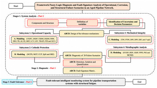
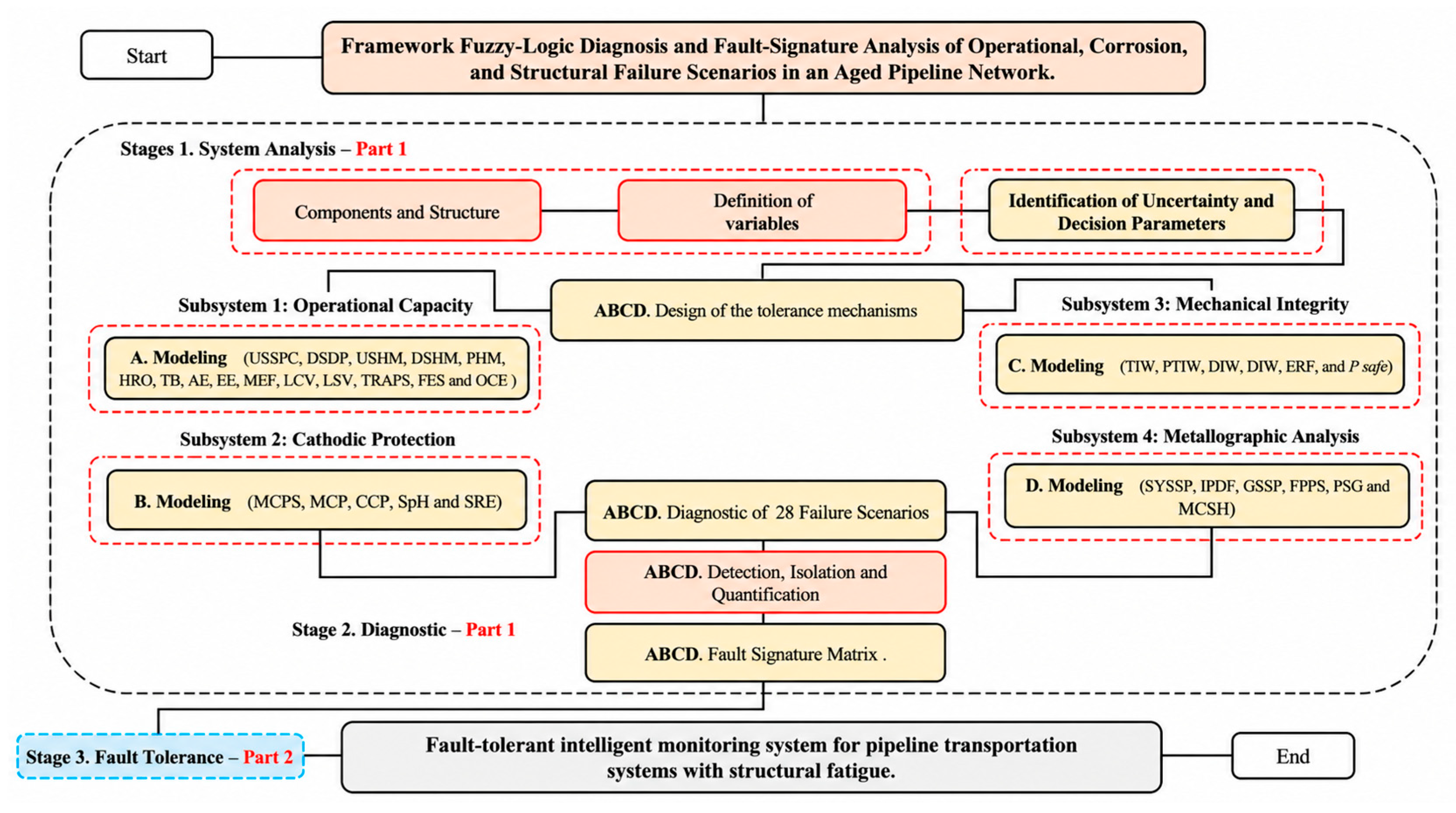
Figure 1 illustrates the methodological structure of this article. Stages 1 and 2 cover the analysis, diagnosis, and modeling of a PTS to develop a remote, non-intrusive, and fault-tolerant intelligent structural fatigue monitoring system. Integrating modules A, B, C, and D supports a predictive control strategy initially applied to offline processes in a virtual environment. Results are presented via a decision-support interface that allows the operator to compare graphically and statistically the model’s behavior with actual system conditions through fault detection, quantification, and isolation. This article presents the proposed architecture for integrating component analysis and diagnosis. A second article will present the system’s reconfiguration, evaluation, and optimization using neuro-fuzzy control and genetic algorithms.

Figure 1. Article methodology.

This study proposes an interpretable framework for diagnosing failure propagation in an aged pipeline network by combining operational, cathodic-protection, mechanical-integrity, and metallurgical information. Unlike conventional approaches that analyze corrosion, structural defects, or operating anomalies independently, the methodology represents 28 failure scenarios using Mamdani fuzzy models and integrates them into a fault-signature matrix. Its originality lies in combining large-scale historical SCADA, SAP, soil, CIPS, ultrasonic-inspection, and material-characterization data with validated expert knowledge to identify localized and system-wide degradation patterns. The framework preserves the traceability of each diagnosis through explicit variables, rules, and residual signatures. This offers greater interpretability than purely data-driven black-box models. Its practical value lies in establishing a structured basis for fault isolation, diagnostic signature breadth, maintenance prioritization, and the future development of neuro-fuzzy reconfiguration and fault-tolerant control strategies in PTS.

3. Results—System Analysis

3.1. Components and Structure

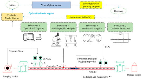
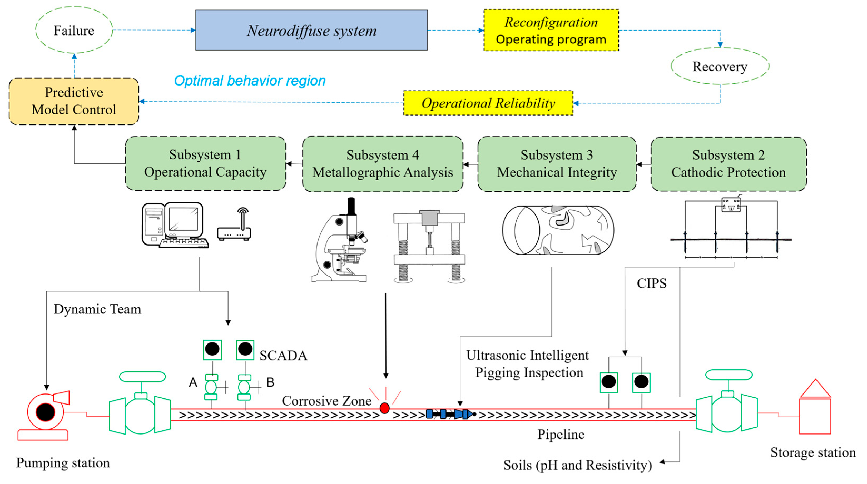
Fault-tolerant control in PTS is a fundamental tool for managing operational integrity in the oil industry. It involves detecting, isolating, and quantifying faults to determine recovery actions and achieve optimal performance within the transportation system. The Intelligent Monitoring System (IMS) evaluates the system through four main subsystems. Subsystem 1 analyzes the operational variables of the PTS linked to SCADA and SAP. Subsystem 2 evaluates the corrosion protection system to determine soil aggressiveness along the right-of-way. Subsystem 3 describes the intelligent ultrasonic inspection used to evaluate the mechanical integrity of the pipeline. Subsystem 4 characterizes the mechanical and microstructural properties of API L X65 steel through metallographic analysis. The graphical structure of the IMS is shown in Figure 2.

Figure 2. Graphical structure of the IMS.

3.1.1. Subsystem 1—Operational Capacity

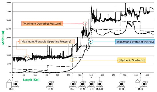
The Mexican oil and gas industry operates a PTS of more than 17,000 km in length, comprising 48 oil pipelines, 78 gas pipelines, 11 polyethylene pipelines, and four mixed pipelines, ensuring the timely supply of hydrocarbons and petrochemical products [17]. The diversity of Mexican crude oil blends, with their particular characteristics detailed in Figure 3, significantly increases the complexity of the transport process.

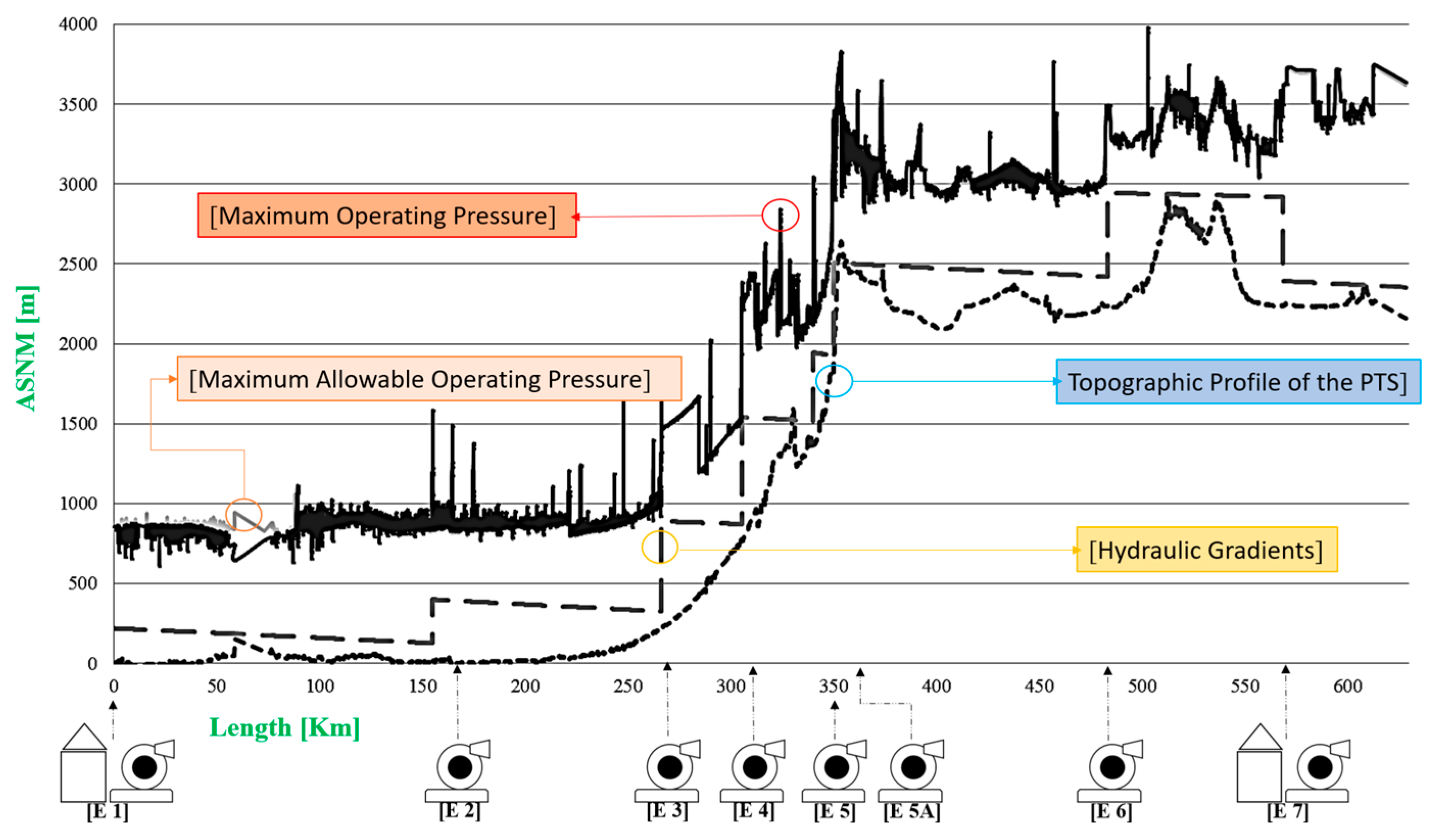
Figure 3. Physicochemical properties of Mexican crude oils and topographic and hydraulic profile of the Mendoza Distribution Center (MDC). Source: Based on [18].

The process begins with the reception of hydrocarbons at pumping station E-1 in Nuevo Teapa, Veracruz (Km 0). The flow continues sequentially through E-2 in Loma Bonita, Oaxaca (Km 166), E-3 in Arroyo Moreno, Veracruz (Km 277), E-4 in Zapoapita, Veracruz (Km 317), and E-5A in Ciudad Mendoza, Veracruz (Km 351). The latter is considered a power station due to the area’s topographic profile. The process continues through E-5 in Maltrata, Veracruz (Km 362), E-6 in San Martín Texmelucan, Puebla (Km 488), and ends at E-7 in Venta de Carpio, State of Mexico (Km 572).

The Mendoza Distribution Center (MDC) faces the challenge of stabilizing the operational reliability of the PTS to prevent hydraulic hammer and cavitation effects in a mechanically deteriorated system with a complex topographic profile. Figure 3 shows the topographic and hydraulic profile for a pumping rate of 150 Thousand Barrels per Day (MBD) on a 24″ Ø line transporting MAYA crude. This crude has a constant viscosity of 21°API and a specific gravity of 0.88 Km/m³, considering the operational limits and the location of the main facilities above sea level.

The case study is developed at the MDC, Veracruz, Mexico, which operates with a program of 140 to 220 MBD [17]. Hydrocarbons are dispatched through 24″ Ø and 30″ Ø pipelines spanning 572 km, using a sequential pumping system driven by six stations assisted by SAP, telemetry, and a SCADA.

The distribution center has infrastructure comprising 96 line-sectioning valves, 17 check valves, 28 pig traps, and remote instrumentation. Table 1 presents the detailed operational capacity.

Table 1. Operational program. Source: Based on [18].

Parameters (Kg/cm2)	E-2	E-3	E-4	E-5A	E-5	E-6
Maximum operating pressure	53	66	79	55	74	63
High discharge pressure alarm	54	67	80	56	75	64
High discharge pressure trip	54.5	67.5	80.5	63	75.5	64.5
Relief valve trip at discharge	55	68	81	63.5	76	65
Low suction pressure alarm	6	6	6	14	5.5	6
Low suction pressure trip	4	4	4	12	4	4
Number of dynamic equipment units	6	6	7	4	7	7
Installed power (HP)	30	30	35	20	35	35

From January to September 2024, Petróleos Mexicanos (PEMEX) recorded 8038 clandestine taps on petroleum and hydrocarbon pipelines nationwide, a 10.34% decrease from the same period in 2023. The frequency of taps was one every 49 min and 3 s for hydrocarbons and one every 8 h and 37 min for liquefied petroleum gas. Hidalgo had the highest number of cases with 1911 taps on hydrocarbon pipelines. Puebla led in liquefied petroleum gas with 354 cases. This article focuses on a 90 km section of the PTS, the E-5 to E-6 segment in Veracruz and Puebla. This area is critical due to its topography and high incidence of hydrocarbon theft.

3.1.2. Design of the Tolerance Mechanisms of Subsystem 1

To develop fault-tolerant control, it is necessary to identify variables associated with faults that disrupt the system. These variables support the diagnostic framework and fault-signature matrix, enabling the adaptive control law to generate appropriate regulations. The developed neuro-fuzzy control model is based on modeling fault scenarios generated by the subsystems’ input variables, allowing a quantitative representation of the associated factors. The fuzzy model interpreted a database with 596 operational observations, each described by fifteen input variables. This produced 8940 scalar measurements that were organized, normalized, and divided into training sets (5364 cases, 60%), validation sets (1788 cases, 20%), and testing sets (1788 cases, 20%).

We defined parameter ranges using a method based on technical standards, corrosivity criteria, and each subsystem’s experimental data. For field variables related to mechanical integrity, cathodic protection, and coating, we aligned the selection of ranges and categories with the pipeline integrity management approach and the technical criteria for cathodic protection and external corrosion control in the ISO 15589-1 standard [17]. These ranges represent levels of technical severity that help prioritize critical areas, interpret risk conditions, and support decision-making on failure scenarios. The standards underpin the measurement method and assessment framework. Specific fuzzy ranges are calibrated using real-world data, the technical literature, and expert judgment. The data are supported by the Comprehensive Rehabilitation Project for the Anticorrosive Protection System of the Nuevo Teapa–Tula–Salamanca oil pipeline (30″, 24″, and 20″ diameters) (PXR-OP-SCC-SUD-GCM-L-13-14). Membership functions were defined for each variable across all subsystems. A rule base was created with “IF … THEN” statements; for example:

Rule = ctrl.Rule (USSPC[‘Low’] if DSDP[‘Out of Operation’] if USHM [‘Low’] if DSHM [‘Regulate’] if PHM [‘Low’] if HRO[‘Moderate’], if TB[‘Moderate’], if AE [‘Low’], if EE [‘Moderate’], MEF [‘Low’], LCV [‘Moderate’], LSV [‘Low’], TRAPS [‘Low’], FES [‘Not’], OCE [‘Yes’], Then FS-1 [‘Out of Operation’]).

These rules were developed using the expert knowledge of 18 certified specialist technicians (Levels 1 and 2) from Pemex Logística and DTsi México. These specialists have experience with AMPP standards, internal corrosion direct assessment (NACE SP0206-2006, NACE SP0208-2008) [15], cathodic protection systems, and the evaluation of coatings and corrosion inhibitors (NRF-005-Pemex-2007) [18].

For subsystem 1, the data were divided, normalized, and the initial model architecture defined. Goodness-of-fit tests and systematic graphical analysis helped understand the behavior of input variables under adverse conditions, based on simulations of possible combinations of associated variables. This facilitates interpreting their combined influence and the system’s sensitivity to fault scenarios. It allows isolating and examining the combined effect of factors in each simulation to improve control. This approach is useful when input parameters lack strict limits and expert knowledge is included through linguistic terms. Fifteen normalized variables within discrete ranges were represented using Gaussian, trapezoidal, triangular, or sigmoid membership functions. The choice depended on their operational behavior (see Table 2A) and failure scenarios (see Table 2B).

Table 2. (A) Input parameters for the linguistic variables of subsystem 1. (B) Output parameters for the linguistic variables of subsystem 1.

(A)
Variable (Inputs)	Linguistic label	Membership Function	Interval
USSPC—Upstream station suction pressure capacity (Kg/cm2).	Out of operation	1-Gamma	(0, 0.01, 3,99, 4.00)
	Low	Trapezoidal	(3.99, 4.01, 18.49, 18.50)
	Average	Triangular	(18.49, 37.50, 55.50)
	High	Gamma	(55.49, 55.51, 75.50, 85.50)
DSDP—Downstream station discharge pressure capacity (Kg/cm2).	Out of operation	1-Gamma	(0, 0.01, 3.99, 4.00)
	Low	Trapezoidal	(3.99, 4.01, 19.99, 20.00)
	Average	Triangular	(19.99, 45.00, 60.00)
	High	Gamma	(59.99, 60.01, 80.50, 90.50)
USHM—Compliance with the upstream station’s historical maintenance program (%).	Out of operation	1-Gamma	(0, 0.01, 9.99, 10.00)
	Low	Gaussian	(9.99, 10.01, 44.99, 45.00)
	Moderate	Triangular	(44.99, 65.00 80.00)
	Desirable	Gamma	(79.99, 80.01, 99.99, 100.00)
DSHM—Compliance with the downstream station’s historical maintenance program (%).	Out of operation	1-Gamma	(0, 0.01, 9.99, 10.00)
	Low	Gaussian	(9.99, 10.01, 44.99, 45.00)
	Regulate	Triangular	(44.99, 65.00 80.00)
	Desirable	Gamma	(79.99, 80.01, 99.99, 100.00)
PHM—Compliance with historical pipeline maintenance between upstream and downstream stations (%).	Out of operation	1-Gamma	(0, 0.01, 9.99, 10.00)
	Low	Gaussian	(9.99, 10.01, 44.99, 45.00)
	Moderate	Triangular	(44.99, 65.00 80.00)
	Desirable	Gamma	(79.99, 80.01, 99.99, 100.00)
HRO—Availability of human resources to operate the station (1:1).	Out of operation	1-Gamma	(0,0.01,0.99,1.00)
	Low	Trapezoidal	(0.99, 1.01,10.99,11.00)
	Moderate	Triangular	(10.99, 22.00, 33.00)
	Desirable	Gamma	(32.99, 33.01, 44.99,45.00)
TB—Availability of dynamic equipment (turbo-pumps) (1:1).	Out of operation	1-Gamma	(0,0.01, 0.99, 1.00)
	Low	Trapezoidal	(0.99, 1.01, 1.99, 2.00)
	Moderate	Trapezoidal	(1.99, 2.01, 3.99, 4.00)
	Desirable	Gamma	(3.99, 4.01, 6.99, 7.00)
AE—Availability of auxiliary equipment—relief valves, alarms, recirculation and storage tanks (%).	Out of operation	1-Gamma	(0, 0.01, 10.99, 11.00)
	Low	Gaussian	(10.99, 11.01, 44.99, 45.00)
	Moderate	Triangular	(44.99, 65.00, 80.00)
	Desirable	Gamma	(79.99, 80.01, 99.99, 100.00)
EE—Availability of emergency equipment and power generators (%).	Out of operation	1-Gamma	(0, 0.01, 14.99, 15.00)
	Low	Gaussian	(14.99, 15.01, 44.99, 45.00)
	Moderate	Triangular	(44.99, 65.00, 80.00)
	Desirable	Gamma	(79.99, 80.01, 99.99, 100.00)
MEF—Availability of measuring equipment, filtration, actuators and flow sensors (%).	Out of operation	1-Gamma	(0, 0.01, 19.99, 20.00)
	Low	Gaussian	(19.99, 20.01, 44.99, 45.00)
	Moderate	Triangular	(44.99, 65.00, 80.00)
	Desirable	Gamma	(79.99, 80.01, 99.99, 100.00)
LCV—Availability of line check valves (1:1).	Out of operation	1-Gamma	(0,0.01, 0.99, 1.00)
	Low	Trapezoidal	(0.99, 1.01, 1.99, 2.00)
	Moderate	Trapezoidal	(1.99, 2.01, 4.99, 5.00)
	Desirable	Gamma	(4.99, 5.01, 5.99, 6.00)
LSV—Availability of line section valves (1:1).	Out of operation	1-Gamma	(0,0.01, 3.99, 4.00)
	Low	Trapezoidal	(3.99, 4.01, 7.99, 8.00)
	Moderate	Trapezoidal	(7.99, 8.01, 15.99, 16.00)
	Desirable	Gamma	(15.99, 16.01, 18.99, 19.00)
TRAPS—Availability of product shipping and receiving traps (1:1).	Out of operation	1-Gamma	(0,0.01, 0.99, 1.00)
	Low	Trapezoidal	(0.99, 1.01, 1.99, 2.00)
	Desirable	Gamma	(1.99, 2.01, 3.99, 4.00)
FES—Interconnection availability for flow enhancer systems.	Not	1-Gamma	(0, 0.01, 0.98, 0.99)
	Yes	Gamma	(1.00, 1.01, 1.98, 1.99)
OCE—Availability of open communication and SCADA equipment.	Not	1-Gamma	(0, 0.01, 0.98, 0.99)
	Yes	Gamma	(1.00, 1.01, 1.98, 1.99)
(B)
Variable (Outputs) Failure Scenarios	Linguistic label	Membership Function	Interval
FS-1—Failure in dynamic equipment of the upstream or pumping station (product discharge or suction—Kg/cm2).	Out of operation	1-Gamma	(0, 0.1, 13.99, 14.00)
	High	Trapezoidal	(13.99, 14.01, 29.99, 30.00)
	Moderate	Trapezoidal	(29.99, 30.01, 69.99, 70.00)
	Low	Gamma	(69.99, 70.01, 84.99, 85.00)
FS-2—Failure in dynamic equipment of the downstream pumping station (product discharge or suction—Kg/cm2).	Out of operation	1-Gamma	(0, 0.1, 13.99, 14.00)
	High	Trapezoidal	(13.99, 14.01, 29.99, 30.00)
	Moderate	Trapezoidal	(29.99, 30.01, 69.99, 70.00)
	Low	Gamma	(69.99, 70.01, 84.99, 85.00)
FS-3—Operational communication problem of the upstream or downstream station.	Intermittent or non-existent	1-Gamma	(0, 0.01, 0.98, 0.99)
	(Yes) Out of operation	Gamma	(1.00, 1.01, 1.98, 1.99)
FS-4—Failure due to exceeding the maximum safe operating pressure for a pipe with a metal loss indicator.	(Not) Low operational risk	1-Gamma	(0, 0.01, 0.98, 0.99)
	(Yes) High operational risk	Gamma	(1.00, 1.01, 1.98, 1.99)
FS-5—Failure in upstream flow sensor or actuator.	(Not) Low operational risk	1-Gamma	(0, 0.01, 0.98, 0.99)
	(Yes) High operational risk	Gamma	(1.00, 1.01, 1.98, 1.99)
FS-6—Failure in downstream flow sensor or actuator.	(Not) Low operational risk	1-Gamma	(0, 0.01, 0.98, 0.99)
	(Yes) High operational risk	Gamma	(1.00, 1.01, 1.98, 1.99)
FS-7—Failure in pipeline instrumentation and safety equipment (sectioning valve, check valves, sending or receiving traps, storage tanks, transfer and fire extinguishing equipment).	(Not) Low operational risk	1-Gamma	(0, 0.01, 0.98, 0.99)
	(Yes) High operational risk	Gamma	(1.00, 1.01, 1.98, 1.99)
FS-8—Leak at pipeline location (hydrocarbon theft).	(Not) Low operational risk	1-Gamma	(0, 0.01, 0.98, 0.99)
	(Yes) High operational risk	Gamma	(1.00, 1.01, 1.98, 1.99)
FS-9—Leak at pipeline location (structural fatigue).	(Not) Low operational risk	1-Gamma	(0, 0.01, 0.98, 0.99)
	(Yes) High operational risk	Gamma	(1.00, 1.01, 1.98, 1.99)

To prevent the combinatorial rule explosion caused by evaluating fifteen operational inputs simultaneously, the original monolithic Mamdani system was decomposed into a hierarchical fuzzy inference structure. The first layer included five local inference systems representing upstream-station condition, downstream-station condition, maintenance and human-resource readiness, instrumentation and isolation capability, and emergency and communication availability. Their outputs were normalized risk indices from 0 to 100, classified as low, acceptable, degraded, or critical. A second diagnostic layer combined only the indices directly linked to each operational failure scenario, generating FS-1 through FS-9. Pressure-related and structural scenarios also received the safe-pressure ratio and structural-fatigue index from the mechanical-integrity subsystem. The hierarchical decomposition reduced the maximum rule base from 201,326,592 Cartesian combinations to about 736 interpretable rules while preserving traceability of the original input variables and failure scenarios. This architecture also allows independent calibration and validation of each local module before integration into the fault-signature matrix.

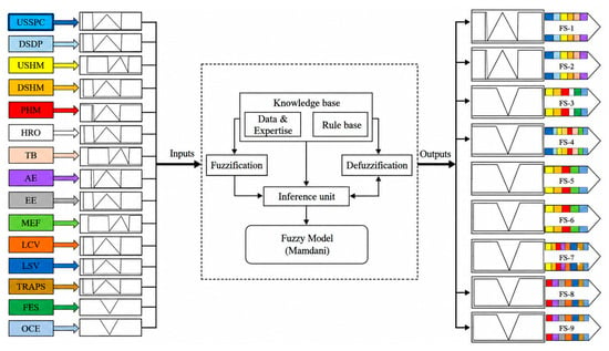
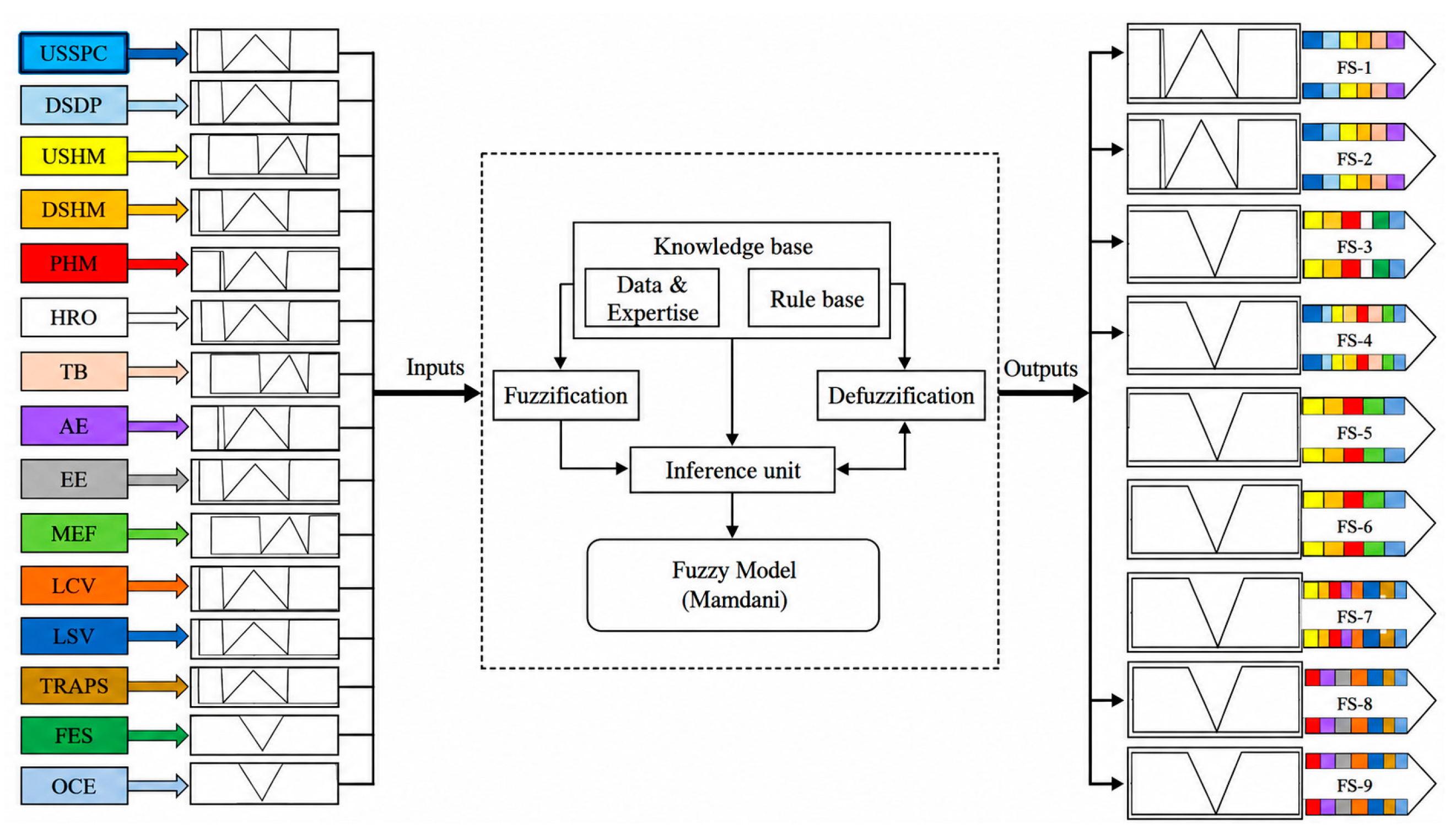
Because the membership functions overlap, a given input vector can activate several rules with varying intensities. Sensitivity, consistency, and redundancy analyses identified rules with negligible activation and equivalent consequents. These rules were developed by consensus with six certified technicians (ECM0301 Risk and Mechanical Integrity Assessment of Pipelines for the Transportation/Collection of Hydrocarbons, Petroleum Products, and Chemicals) from Pemex Logistic. Figure 4 shows the architecture of fuzzy system one and the interaction between the input variables and the modeled failure scenarios.

$$N_{\mathit{rules}}{\prod }_{i=1}^n{m}_i$$

(1)

Figure 4. Architecture of the first fuzzy model.

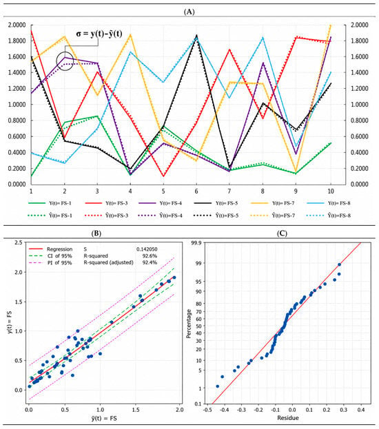
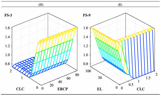
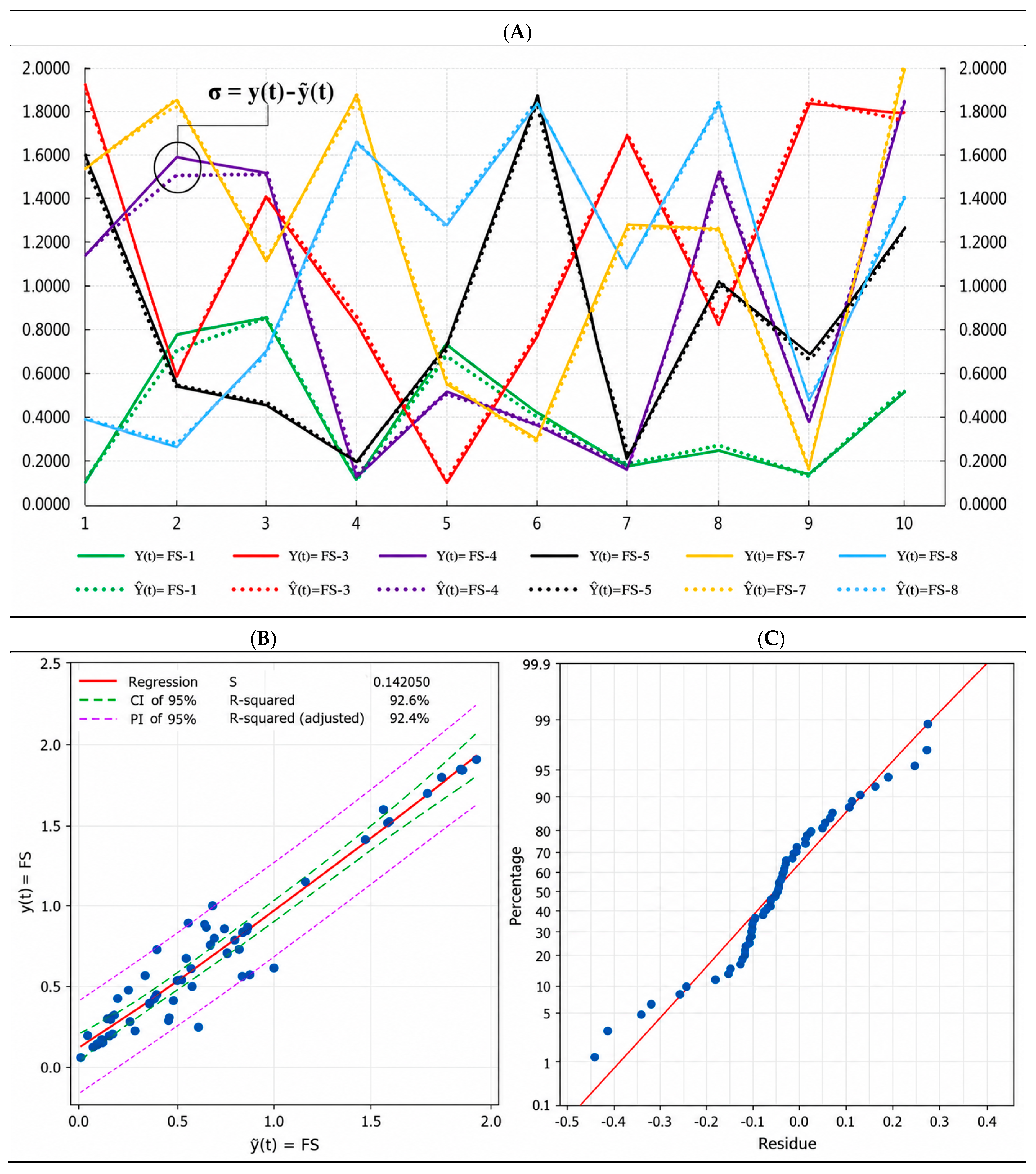
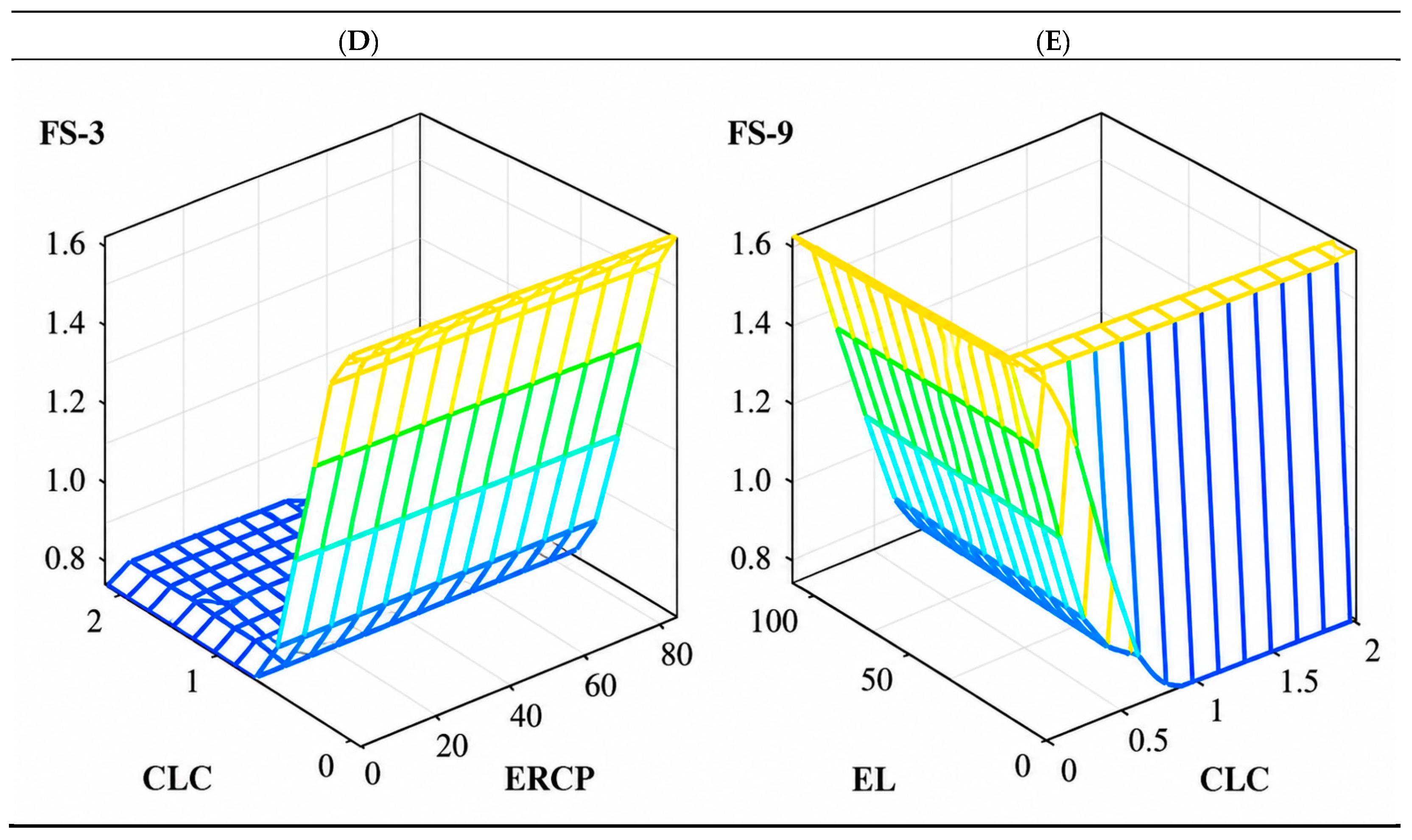
The reliability of subsystem 1 was validated using real-system data and fuzzy model estimates to identify variability in the normalized outputs. Figure 5 presents a sample of six real and estimated failure scenarios, with 600 data points defined by a factorial experimental design. Figure 5A shows a magnified view of the variable behavior, allowing visual identification of its variance, which ranged from 2.16 to 9.21. The regression analysis showed strong agreement between experimental and predicted ỹ (t) = FS values, with an RMSE of 92.6%, MAE 91.8% and an adjusted R² of 92.4%. The standard error of the regression was 0.14205, indicating small deviations between predicted and observed values. Most observations were close to the regression line and within the 95% prediction interval [B]. The normal probability plot of the residuals showed an approximately linear distribution, with minor deviations at the extreme tails. These results indicate adequate goodness-of-fit and suggest the normality assumption of the residuals is reasonably satisfied [C]. The response surface diagrams represent the graphical behavior of the system under fuzzy inference rules. Figure 5D shows that when the permissible operating limits of a pipeline with metal loss indicators (MAOP) are exceeded, the failure scenario (FS-4) increases because the average discharge pressure capacity (55.50 kg/cm²), established by the ANSI/ASME B31G standard for a downstream station (DSDP), is exceeded and the open communication and SCADA (OCE) system for controlling and monitoring operating conditions is unavailable. Indicators below 1.0 increase the likelihood of system failure. Figure 5E shows the activation of failure scenarios (FS-8), triggered by leaks at a pipeline location due to hydrocarbons. This is represented by the variables (EE) and (OCE). These relate to the availability of emergency equipment and auxiliary power generators, as well as open communication and remote-control equipment in case of a product spill emergency. The indicators decrease to 100% and below 1.0, respectively, for the variables that increase the incidence of scenario failures, while indicators above 1.0 indicate the incidence of product leaks at a pipeline location.

Figure 5. (A) Validation and comparison of the fuzzy model for subsystem 1. (B,C) Analysis and comparison of the standard error of the regression. (D,E) Response surface diagrams for FS-3 and FS-9.

3.1.3. Subsystem 2—Cathodic Protection

This corresponds to the comprehensive rehabilitation project of the anticorrosive protection system for the 24″–30″ Ø pipeline, Nuevo Teapa–Venta de Carpio section (572 km). The evaluation includes CIPS, DCVG studies, localization of electrical shunts using PCM equipment, and analysis of soil pH and resistivity along the right-of-way (PXR-OP-SCC-SUD-GCM-L-13-14). Soil is the most complex electrolyte here, with pH and resistivity as the key parameters to quantify its corrosive aggressiveness. pH values below 5.5 indicate acidic conditions that accelerate metallic corrosion, showing a direct correlation between higher acidity and greater aggressiveness.

Resistivity (ρ), for its part, measures the opposition of the soil to the flow of electric charge and is expressed through the generalized Ohm’s Law:

ρ = R (A/L)

(2)

R is the electrical resistance (Ω), A is the cross-sectional area (cm²), and L is the distance between electrodes (cm). The electrochemical current causing corrosion is estimated as:

I = V · A/ (ρ L)

(3)

This expression shows soil corrosivity is inversely proportional to resistivity (Corrosivity ∝ 1/ρ): the lower the ρ, the greater the ionic conductivity and the higher the galvanic corrosion rate. Based on experimental correlations between measured ρ values and corrosion rates in buried pipelines, empirical classification ranges are established and shown in Table 3.

Table 3. Degree of soil aggressiveness as a function of resistivity. Source: [14].

Soil Corrosivity	Soil Resistivity (Ωcm)
Highly Corrosive	<1000
Corrosive	1001–5000
Slightly Corrosive	5001–10,000
Very Slightly Corrosive	>10,001

The CIPS study is an indirect inspection technique that determines the level of cathodic protection of a buried or submerged pipeline using a metallic structure detector, voltage rectifiers, and GPS. Pipe-to-soil potentials are recorded with the current switched on and off at every meter, following established regulations [14].

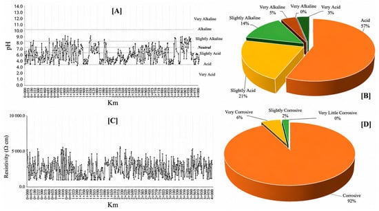
The results of the soil resistivity and pH study along the right-of-way (ROW) are divided into sections called segments. Segment No. 9 covers soils from E-5 to E-6. Figure 6 shows the pH profile along the segment, with pH values on the “y” axis at each distance point on the “x” axis [A]. A total of 907 soil readings were conducted from Km 408 to Km 498. The classification of results [B] determines an average soil pH of 5.8. The soil resistivity survey shows the calculated resistivity value on the “y” axis at each distance point on the “x” axis [C]. With 907 soil readings, the classification of results [D] determines an average soil resistivity of 2506.1 Ω-cm.

Figure 6. pH and resistivity studies of Segment No. 9. (A) pH profile (y-axis) vs. distance (x-axis); (B) classification of pH results (average pH = 5.8); (C) soil resistivity profile; (D) classification of resistivity results (average = 2506.1 Ω-cm). Source: Based on [19].

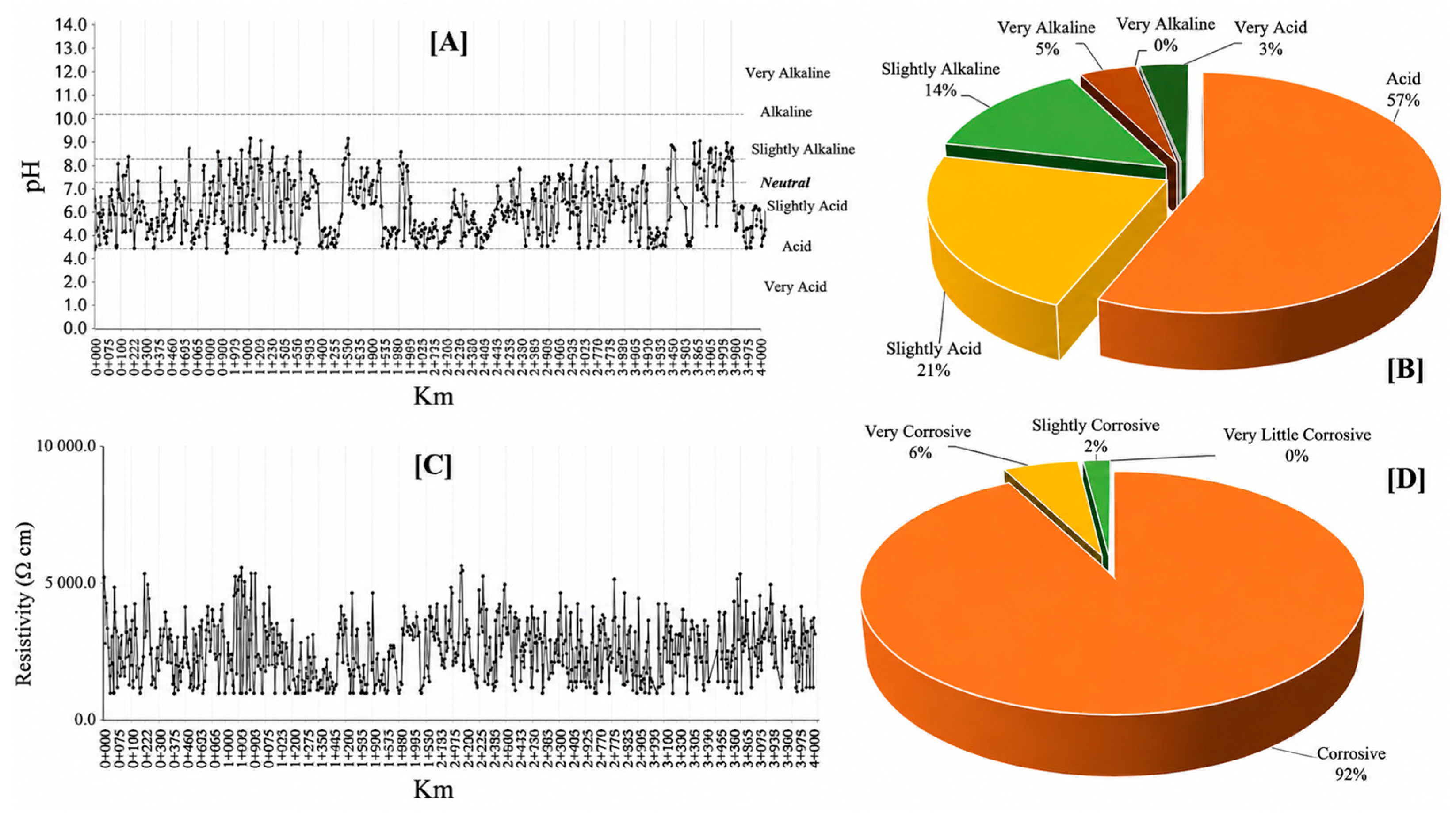
According to the above data and the general study of the PTS, the percentage of recorded data is illustrated in Figure 7, showing that acidic and slightly acidic pH values are present in equal proportion [A], alongside highly corrosive and corrosive soil [B]. This must be considered when assessing the level of cathodic protection and the condition of the mechanical coating, since the aggressive nature of the soil affects the coating’s state.

Figure 7. pH, resistivity, and CIPS studies. (A) Proportion of acidic/slightly acidic pH values; (B) proportion of highly corrosive/corrosive soil; (C) CIPS study of Segment No. 9. (D) and total study results (E); Source: Based on [20].

The CIPS study of Segment No. 9 is shown in graph [C], influenced by five rectifiers (RPC) with significant differences in potential and resistance. Several fall below the reference threshold of −850 millivolts (mV) set by regulations [17], NACE-SP0169-2013 [19]. Based on the difference between On and Off (interruption) potentials, 82.90% of data points are above the −100 mV interruption threshold.

3.1.4. Design of the Tolerance Mechanisms of Subsystem 2

For subsystem 2, the data were divided and normalized, and the initial model architecture was defined. Goodness-of-fit tests and graphical analysis helped us to understand the behavior of input variables under adverse conditions. This was based on simulations of possible combinations of associated variables. Five normalized variables within discrete ranges were represented by membership functions according to their behavior, along with five failure scenarios (see Table 4).

Table 4. Parameters for the linguistic variables of subsystem 2.

Variable (Inputs)	Linguistic Label	Membership Function	Interval
MCPS—Compliance with the maintenance of the cathodic protection system (%).	Low	1-Gamma	(0, 0.01, 44.99, 45.00)
	Regular	Trapezoidal	(44.99, 45.01, 79.99, 80.00)
	Desirable	Gamma	(79.99, 80.01, 99.99, 100.00)
MCP—Conditions of the mechanical coating of the pipeline (%).	Low	1-Gamma	(0, 0.01, 44.99, 45.00)
	Regular	Trapezoidal	(44.99, 45.01, 84.99, 85.00)
	Desirable	Gamma	(84.99, 85.01, 99.99, 100.00)
CCP—Current level of cathodic protection (%).	Low	1-Gamma	(0, 0.01, 49.99, 50.00)
	Regular	Trapezoidal	(49.99, 50.01, 79.99, 80.00)
	Desirable	Gamma	(79.99, 80.01, 99.99, 100.00)
SpH—Soil acidity level (H±).	Acidic	1-Gamma	(0, 0.01, 6.98, 6.99)
	Neutral	Triangular	(6.99, 7.00 7.99)
	Alkaline	Gamma	(7.99, 8.00, 13.99, 14.00)
SRE—Soil aggressiveness based on its resistivity (Ωcm).	Highly	1-Gamma	(0, 0.01, 999.99, 1000.00)
	Average	Gaussian	(999.99, 1000.01, 4999.99, 5000.00)
	Slightly	Gaussian	(4999.99, 5000.01, 9999.99, 10,000.00)
	Very little	Gamma	(9999.99, 10,000.01, 14,999.99, 15,000.00)
Variable (Outputs) Failure Scenarios
FS-10—Voltage rectifier failure, potential variability and electrical bridges (%).	Low corrosive risk	1-Gamma	(0, 0.1, 14.99, 15.00)
	Moderate	Trapezoidal	(14.99, 15.01, 74.99, 75.00)
	High corrosive risk	Gamma	(74.99, 75.01, 99.99, 100.00)
FS-11—Failure in anode bed, anodes, cathodes, connections and conductors (%).	Low corrosive risk	1-Gamma	(0, 0.1, 19.99, 20.00)
	Moderate	Trapezoidal	(19.99, 20.01, 64.99, 65.00)
	High corrosive risk	Gamma	(64.99, 65.01, 99.99, 100.00)
FS-12—Failure in mechanical coating of the oil pipeline.	(Not) Low corrosive risk	1-Gamma	(0, 0.01, 0.98, 0.99)
	(Yes) High corrosive risk	Gamma	(1.00, 1.01, 1.98, 1.99)
FS-13—Failure due to corrosive aggressiveness of the soil (%).	Low corrosive risk	1-Gamma	(0, 0.1, 9.99, 10.00)
	Moderate	Trapezoidal	(9.99, 10.01, 69.99, 70.00)
	High corrosive Risk	Gamma	(69.99, 70.01, 99.99, 100.00)
FS-14—Failure due to corrosive soil resistivity (%).	Low corrosive risk	1-Gamma	(0, 0.1, 24.99, 25.00)
	Moderate	Trapezoidal	(24.99, 25.01, 79.99, 80.00)
	High corrosive risk	Gamma	(79.99, 80.01, 99.99, 100.00)

The fuzzy model analyzed a database with 907 cathodic observations, each described by five input variables. It produced 4535 scalar measurements that were organized and normalized. These were divided into training sets (2721 cases, 60%), validation sets (907 cases, 20%), and testing sets (907 cases, 20%). A total of 324 inference rules were evaluated, corresponding to the Cartesian product of the linguistic categories assigned to the five input variables. Sensitivity, consistency, and redundancy analyses identified rules with negligible activation and equivalent consequents. These rules were developed by consensus with 18 Level 1 and 2 certified technicians from Pemex Logístic and DTsi México. They specialize in AMPP standards, direct internal corrosion assessment (NACE SP0206-2006, NACE SP0208-2008) [15], cathodic protection systems, and the evaluation of coatings and corrosion inhibitors (NRF-005-Pemex-2007) [18].

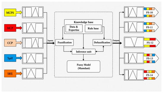
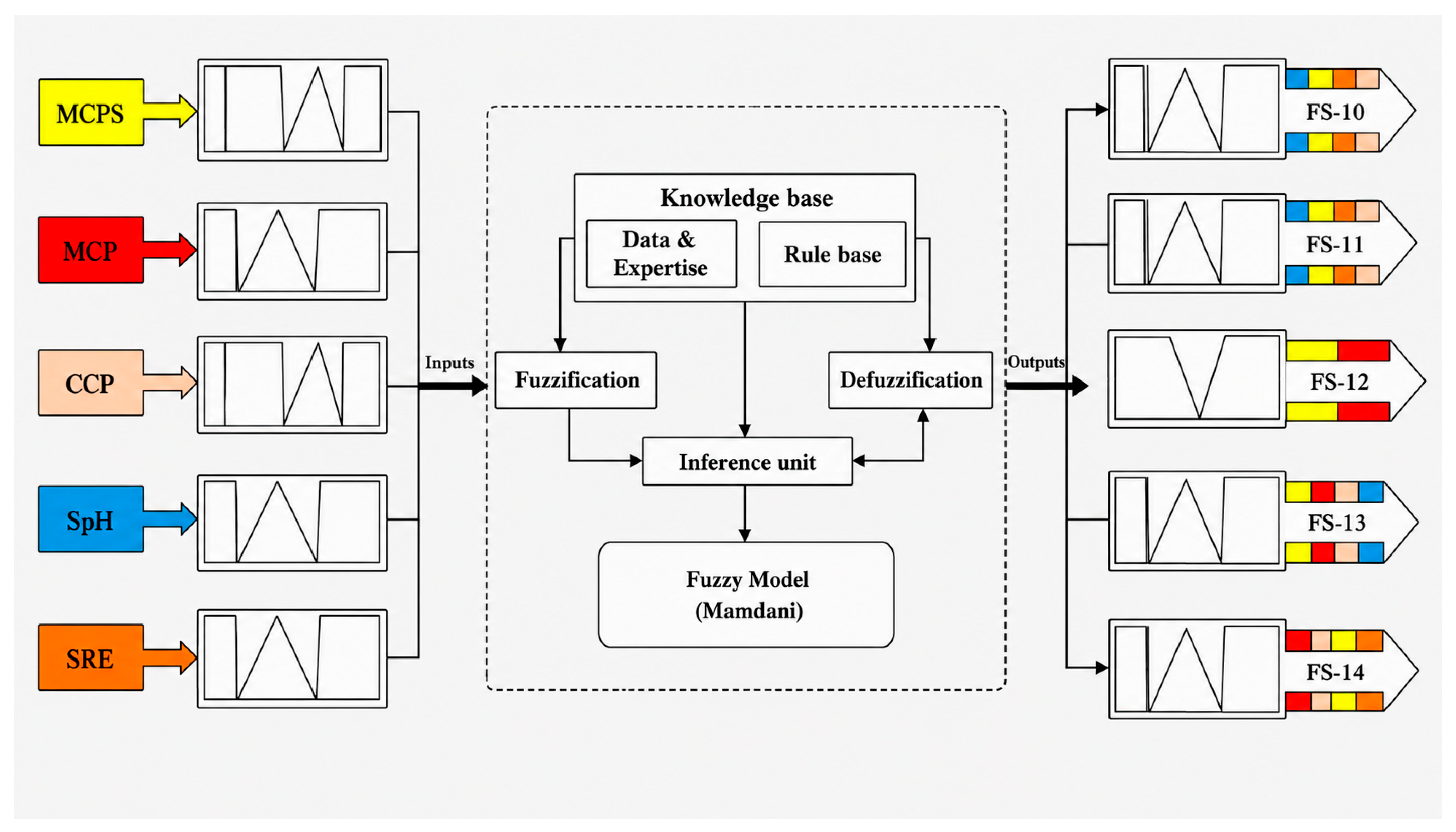
Figure 8 presents the architecture of fuzzy system two and the interaction between the input variables and the modeled failure scenarios.

Figure 8. Architecture of the second fuzzy model.

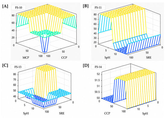
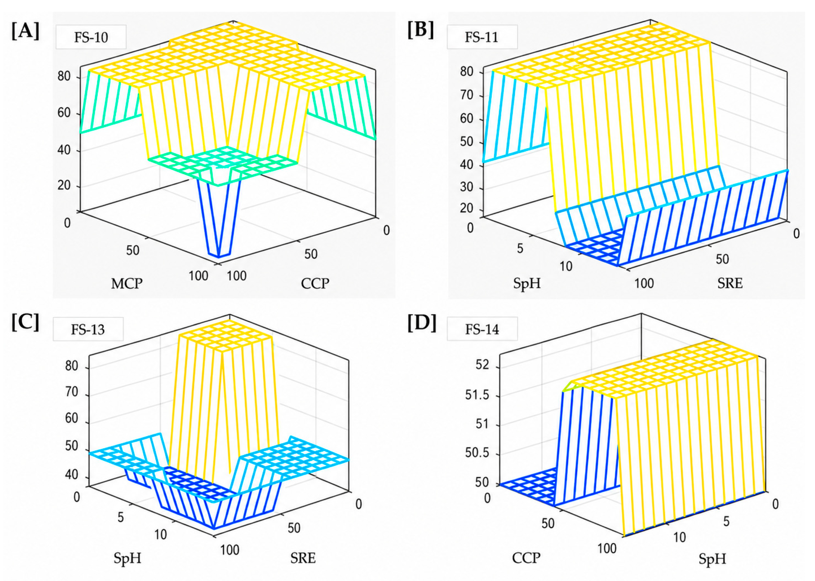
The reliability of subsystem 2 was validated using real system data and fuzzy model estimates to identify variability in normalized outputs, similar to subsystem 1, with variance ranges between 0.98 and 4.73. The regression analysis showed strong agreement between experimental and predicted ỹ (t) = FS values, with an RMSE of 94.8%, MAE 92.4% and an adjusted R² of 94.6%. The standard error of the regression was 0.11809, indicating small deviations between predicted and observed values. Most observations were close to the regression line and within the 97% prediction interval. Figure 9 shows the response surface diagrams. Graph [A] represents the activation of FS-10, which decreases to zero if MCP and CCP variables are at optimal levels; otherwise, failure recurs. [B] The SpH variable shows that soils with pH below 5.5 are acidic and rapidly cause corrosion in bare steel. This is amplified by a deficient mechanical coating on at least 40% of the pipe (SRE), causing exponential activation of FS-11. [C] Soil Corrosive Aggressiveness Failure (FS-13) can be controlled with alkaline indicators (pH above 5.5) and desirable SRE indicators; otherwise, its activation increases. [D] The level of cathodic protection (CCP) and soil acidity (SpH) are key variables for reducing the high corrosive risk caused by soil resistivity to electrical charge flow (FS-14).

Figure 9. Validation and comparison of the fuzzy model of subsystem 2; FS 10 = MCP vs CCP (A); FS 11 = SpH vs SRE (B); FS 13 = SpH vs. SRE (C); FS 14 = CCP vs. SpH (D).

3.1.5. Subsystem 3—(Ultrasonic Intelligent Pigging Inspection)

The mechanical integrity study (MIS) segment in 10 sections was conducted on the 24″–30″ Ø pipeline, Nuevo Teapa–Venta de Carpio section (572 km), from E-1 to E-7, using a straight-beam ultrasonic inspection tool with radially directed sensors to detect pipe wall defects. The analysis of Segment 9 revealed 4651 metal loss indications, 151 geometry defects, 22 mid-wall defects, and 837 anomalies [21,22,23].

The first principal component represents 39% of the total variance. The variables most highly correlated with the first principal component (PC1) are PTIW (0.461), LEIW (0.502), and DIW. The first three principal components account for 73.8% of the data variation. Table 5 shows the principal component analysis (PCA) of Segment 9 [15].

Table 5. PCA of segment 9.

Component Analysis Subsystem 3
Eigenvalue	2.3422	1.2225	0.8607	0.6261	0.5263	0.4221
Proportion	0.390	0.204	0.143	0.104	0.088	0.070
Cumulative	0.390	0.594	0.738	0.842	0.930	1.000
Variable	PC1	PC2	PC3	PC4	PC5	PC6
ERF	0.514	−0.013	−0.259	−0.218	−0.542	−0.572
TIW	−0.192	−0.673	0.506	0.333	−0.304	−0.225
PTIW	0.461	0.026	−0.242	0.837	0.052	0.156
LEIW	0.502	−0.224	0.255	−0.309	−0.245	0.691
DIW	0.483	−0.085	0.407	−0.124	0.679	−0.343
WALL	0.028	0.699	0.623	0.172	−0.301	−0.053

3.1.6. Design of the Tolerance Mechanisms of Subsystem 3

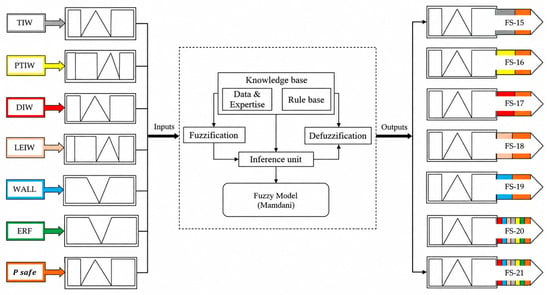
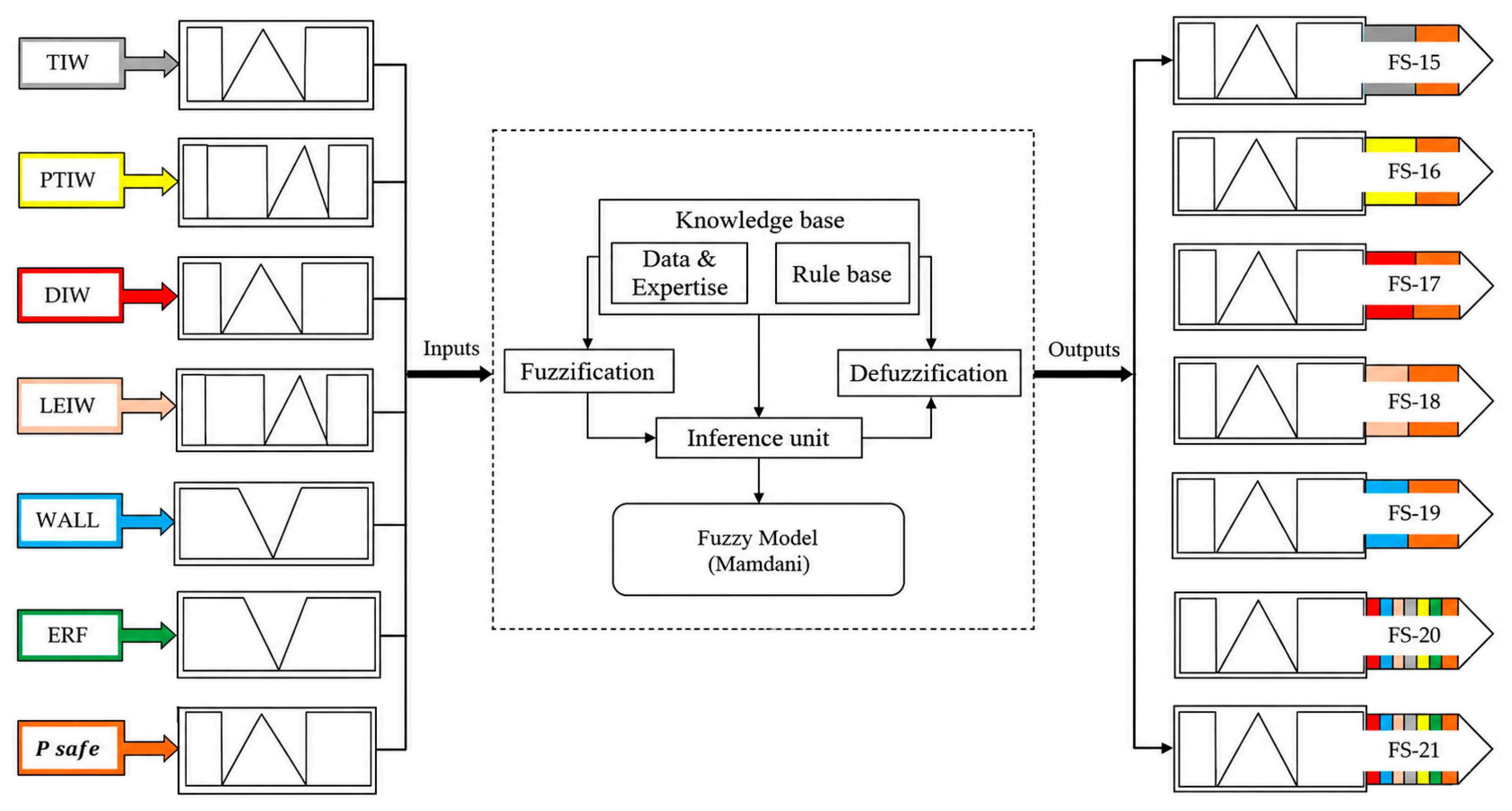
For subsystem 3, the data were divided and normalized, and the initial model architecture was defined. Goodness-of-fit tests and graphical analysis helped us to understand the behavior of input variables under adverse conditions. This was based on simulations of possible combinations of associated variables. Seven normalized variables within discrete ranges were represented by membership functions according to their behavior, along with five failure scenarios (See Table 6).

Table 6. Parameters for the linguistic variables of subsystem 3.

Variable (Inputs)	Linguistic Label	Membership Function	Interval
TIW—Nominal thickness of the internal wall of the pipeline (mm).	Low loss	1-Gamma	(0, 0.01, 4.99, 5.00)
	Considerable loss	Trapezoidal	(4.99, 5.01, 14.99, 15.00)
	High loss	Gamma	(14.99, 15.01, 19.99, 20.00)
PTIW—Percentage of thinning of the internal wall of the pipeline (%).	Low weight loss	1-Gamma	(0, 0.01, 29.99, 30.00)
	Significant weight loss	Trapezoidal	(29.99, 30.01, 59.99, 60.00)
	High weight loss	Gamma	(59.99, 60.01, 99.99, 100.00)
DIW—Defects in the internal wall of the pipeline (mm).	Low discontinuity	1-Gamma	(0, 0.01, 1999.99, 2000.00)
	Considerable discontinuity	Trapezoidal	(1999.99, 2000.01, 3999.99, 4000.00)
	High discontinuity	Gamma	(3999.99, 4000.01, 7999.99, 8000.00)
LEIW—Length of the encrustation on the inner wall of the pipeline (mm).	Small (low risk of fracture)	1-Gamma	(0, 0.01, 999.99, 1000.00)
	Considerable risk of fracture	Triangular	(999.99, 1500.00 2000.00)
	Wide (high risk of fracture)	Gamma	(1999.99, 2000.01, 2999.99, 3000.00)
WALL—Corrosive damage to the internal (+1) or external (−1) wall of the pipeline (+/-).	Internal (+)	1-Gamma	(0, 0.01, 00.99, 1.00)
	External (-)	Gamma	(0, −0.01, −00.99, −1.00)
ERF—Estimated repair factor for a pipe with metal loss indicators (1:1).	<1 (low ERF)	1-Gamma	(0, 0.01, 00.99, 1.00)
	>1 (high ERF)	Gamma	(00.99, 1.01, 2.99, 3.00)
P safe—Maximum safe pressure for a pipeline with metal loss indicators (Kg/cm2).	Low	1-Gamma	(0, 0.01, 19.99, 20.00)
	Reliable	Triangular	(19.99, 45.00, 60.00)
	Critical	Gamma	(59.99, 60.01, 80.50, 90.50)
Variable (Outputs) Failure Scenarios
FS-15—Failure by TIW (%).	Minimal (low operational risk)	1-Gamma	(0, 0.1, 24.99, 25.00)
	Considerable	Trapezoidal	(24.99, 25.01, 74.99, 75.00)
	Critical (high operational risk)	Gamma	(74.99, 75.01, 99.99, 100.00)
FS-16—Failure by PTIW (%).	Minimal (low operational risk)	1-Gamma	(0, 0.1, 19.99, 20.00)
	Considerable	Trapezoidal	(19.99, 20.01, 64.99, 65.00)
	Critical (high risk of fracture)	Gamma	(64.99, 65.01, 99.99, 100.00)
FS-17—Failure by DIW (%).	Minimal (low operational risk)	1-Gamma	(0, 0.1, 29.99, 30.00)
	Considerable	Trapezoidal	(29.99, 30.01, 64.99, 65.00)
	Critical (high operational risk)	Gamma	(64.99, 65.01, 99.99, 100.00)
FS-18—Failure by LEIW (%).	Minimal (low operational risk)	1-Gamma	(0, 0.1, 39.99, 40.00)
	Considerable	Trapezoidal	(39.99, 40.01, 79.99, 80.00)
	Critical (high operational risk)	Gamma	(79.99, 80.01, 99.99, 100.00)
FS-19—Failure by WALL (%).	Low corrosive concentration	1-Gamma	(0, 0.1, 29.99, 30.00)
	Considerable concentration	Trapezoidal	(29.99, 30.01, 69.99, 70.00)
	Wide corrosive concentration	Gamma	(69.99, 70.01, 99.99, 100.00)
FS-20—Failure by ERF (%).	ERF-Low (minimal operational risk)	1-Gamma	(0, 0.1, 24.99, 25.00)
	ERF- Considerable risk of fracture	Trapezoidal	(24.99, 25.01, 59.99, 60.00)
	ERF-High (critical operational risk)	Gamma	(59.99, 60.01, 99.99, 100.00)
FS-21—Failure due to mechanical deterioration in a section of the pipeline (%).	Minimal (low operational risk)	1-Gamma	(0, 0.1, 29.99, 30.00)
	Considerable	Trapezoidal	(29.99, 30.01, 59.99, 60.00)
	Critical (high operational risk)	Gamma	(59.99, 60.01, 99.99, 100.00)

The fuzzy model analyzed a database with 4651 mechanical integrity observations, each described by seven input variables. It produced 32,557 scalar measurements that were organized, normalized, and split into training sets (19,535 cases, 60%), validation sets (6511 cases, 20%), and testing sets (6511 cases, 20%). A total of 972 inference rules were evaluated, corresponding to the Cartesian product of the linguistic categories assigned to the seven input variables. Sensitivity, consistency, and redundancy analyses identified rules with negligible activation and equivalent consequents. These rules were developed by consensus with 18 Level 1 and 2 certified technicians from Pemex Logístic and DTsi México. They specialize in AMPP standards, direct internal corrosion assessment (NACE SP0206-2006, NACE SP0208-2008) [15], cathodic protection systems, and the evaluation of coatings and corrosion inhibitors (NRF-005-Pemex-2007) [18]. Figure 10 presents the architecture of the third fuzzy system and the interaction between the input variables and the modeled failure scenarios.

Figure 10. Architecture of the third fuzzy model.

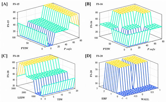
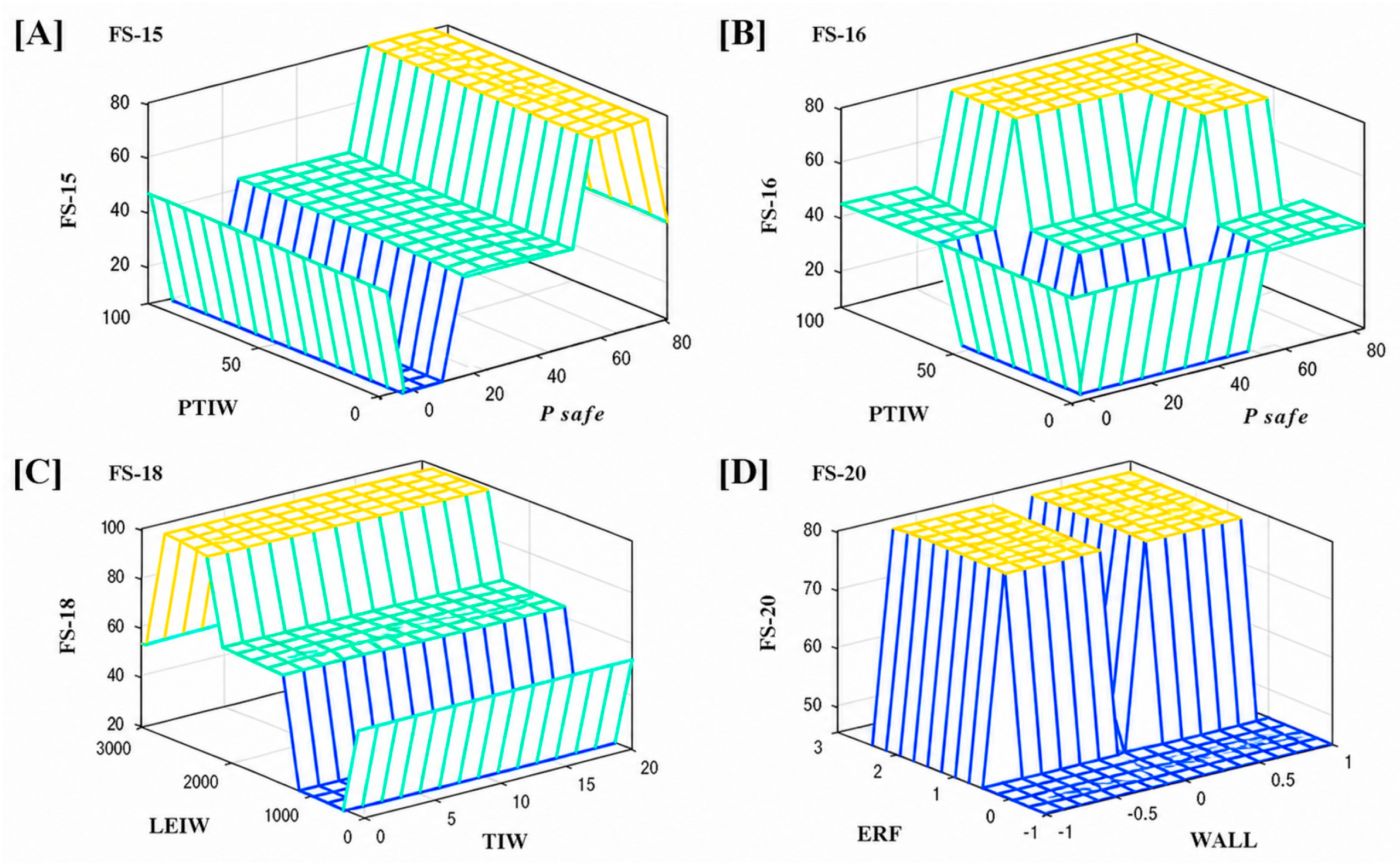
The reliability of subsystem 3 was validated using real system data and fuzzy model estimates to identify variability in the normalized outputs, similar to subsystem 1, with variance ranges between 0.93 and 4.77. The regression analysis showed strong agreement between experimental and predicted ỹ (t) = FS values, with an RMSE of 94.5%, MAE 92.1% and an adjusted R² of 94.0%. The standard error of the regression was 0.11261, indicating small deviations between predicted and observed values. Most observations were close to the regression line and within the 96.7% prediction interval. Figure 11 shows the response surface plots. [A] At low Psafe values, the FS-15 output stays between low and intermediate levels and is sensitive to PTIW. As Psafe rises to a critical region, the output abruptly increases and reaches a high level near 80. Beyond this threshold, PTIW’s effect diminishes, and FS-15 remains in a critical state. This shows Psafe is the dominant variable activating the high state of FS-15. [B] The FS-16 output shows a low output region when both variables are at certain lower intervals, surrounded by intermediate response zones. The combination of high PTIW and/or Psafe values leads to an upward trend, showing no single variable acts completely independently. [C] The FS-18 output has three clearly differentiated activation levels that increase stepwise: low, intermediate, and high. For low LEIW values, FS-18 stays around 20–40; as LEIW increases, the response moves to an intermediate region near 50–60 and finally reaches a high plateau near 100. Although TIW shifts some transitions, LEIW has the greatest influence on the output. [D] The FS-20 surface shows binary behavior. At low ERF values, the output stays near 40 for much of the WALL interval. When ERF exceeds a threshold, FS-20 abruptly changes to a high region near 80. Thus, ERF is the main activation variable, while WALL conditions the response’s specific configuration.

Figure 11. Validation and comparison of the fuzzy model of subsystem 3; FS 15 = PTIW vs P Safe (A); FS 16 = PTIW vs P Safe (B); FS 18 = LEIW vs TIW (C); FS 20 = ERF vs WALL (D).

3.1.7. Subsystem 4—Metallographic Analysis

This section presents the metallographic analysis of an out-of-service underground pipeline with over 75 years of operation to manage generational knowledge of corrosive patterns in land-based pipelines. The module integrates metallographic analysis, chemical etching, roughness analysis, ultrasonic thickness measurement, and tensile testing. The physical and chemical characteristics were compared against current national and international regulations enabling a specific characterization of API L X65 steel [24,25,26,27].

The study sample was extracted from a segment of a 24″ Ø pipeline with a wall thickness between 8 and 11 mm, located in the municipality of Esperanza, Puebla, Mexico. The extraction took place in June 2023 after an emergency response to a hydrocarbon spill. Visually, the sample showed cracks, dents, generalized corrosion, and residuals of a protective coating designed for high-humidity and corrosive environments.

The longitudinal and transverse metallographic probes extracted from the segment were encapsulated in bakelite at 190 °C and 23 kN for 9 min. They were progressively polished with sandpapers of different grit sizes and finally polished with a 0.3 μm alumina solution at 300 RPM until a mirror-like surface was obtained. To reveal the steel microstructure, chemical etching with 1% Nital was applied for 25 s per probe.

Scanning electron microscopy (SEM) analysis at magnifications of up to 50 μm revealed in the API L X65 steel a ferritic–pearlitic microstructure with heterogeneous phase distribution, where pearlite acts as a cathode relative to ferrite, promoting localized dissolution of the material. The determined pearlite phase percentage was 1.039%, a condition that makes the material susceptible to stress corrosion cracking processes.

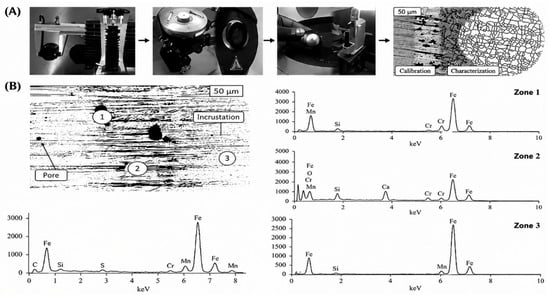
Grain size was calculated using the linear intercept method in accordance with ASTM E-112 standard, yielding an ASTM grain size No. 9 (Figure 12A).

Figure 12. (A) Methodology for extraction and preparation of the metallographic sample, micrographic process, and chemical composition of the steel by zones (B). Source: Based on [25].

The chemical composition analysis (Figure 12B) identified the steel as a high-carbon alloy (6.33 wt%) with iron as the main component (90.07 wt%), obtained at 20.0 kV. The chemical elements were uniformly distributed throughout the analyzed matrix, as detailed in Section [B1] for zones 1, 2, and 3. The chemical composition of the sample is presented in Table 7.

Table 7. Chemical components with reference to weights and atoms.

Element	Weight (%)	Atoms (%)
CK	6.33	20.62
Si K	0.96	1.79
Cr K	0.71	0.94
Mn K	1.93	1.22
Fe K	90.07	75.43
Total	100.00	100.00

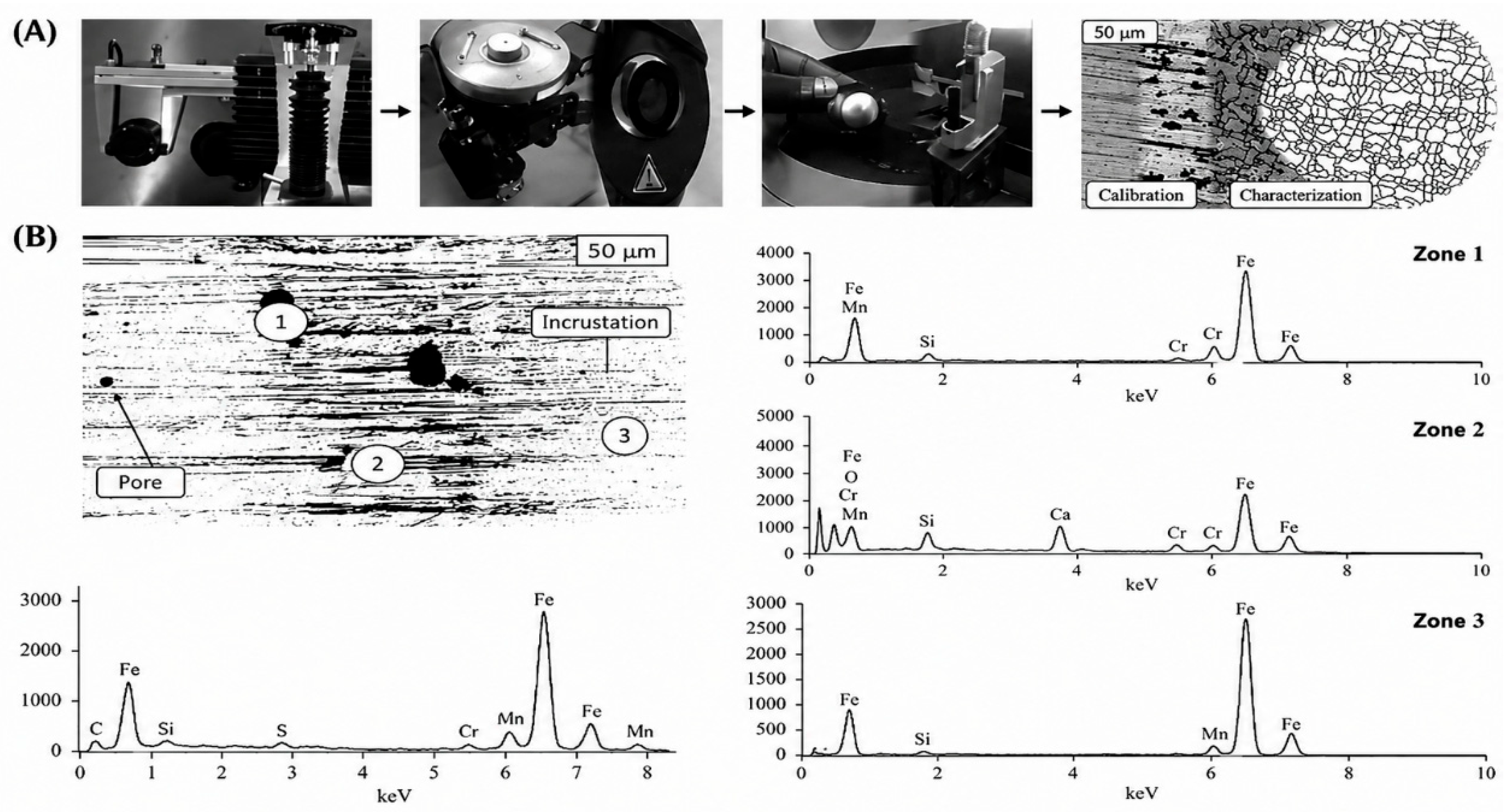
The tensile test was carried out to obtain the mechanical properties and determine the steel grade [26]. Illustration [A] in Figure 13 shows the dimensions under the ASTM E8/E8M standard of two probes used in these tests and the results obtained continuously [27]. Table 8 shows the length, width, and thickness measurements for each probe before testing, as well as their final characteristics. Probes 1 and 2 exhibit pitting or cracks from corrosion, indicating material fatigue. Six probes were used; only two representative probes are presented due to similar results and paper length constraints.

Figure 13. Graphs related to the tensile test. (A) Probe dimensions under ASTM E8/E8M standard; (B) elongation–time relationship for Probe 1 (4.09 mm over 83 s); (C) load–deformation relationship; (D) yield and ultimate tensile strength results for both probes. Source: Based on [25,27].

Table 8. Probe characteristics.

Units	Thickness (mm)	Width (mm)	Calibrated Length (mm)
T01	3.050	13.200	50.000
T02	3.060	13.200	50.000
Final Characteristics:
Probe ID	Max. Thickness (mm)	Max. Width (mm)	Max. Length
T01	2.40	10.28	56.00
T02	2.45	10.30	56.10

Probe 1: This probe shows a linear elongation–time relationship [B]. Over 83 s, it elongates up to 4.09 mm. Illustration [C] shows the load–deformation relationship for the same probe. The tensile test results showed the sample has a yield strength of 394 megapascals (MPa) and a tensile strength of 501 MPa [D] on average.

Probe 2: The elongation–time graph for this probe is also linear, likely because it is an isotropic material [C]. Minimal variation in results was obtained, with a yield strength of 404 MPa and an ultimate tensile strength of 517 MPa [D]. The overall results for both probes are shown in Table 9.

Table 9. Results of the tensile test.

Probe ID	Elongation (%)	Yield Strength		UTS		Ơy/UTS
		MPa	Psi	MPa	Psi
T01	4.09	394	57,144	501	72,663	0.78
T02	5.6	404	58,595	517	74,984	0.78
Average	4.8	399	58,870	509	73,824	0.78

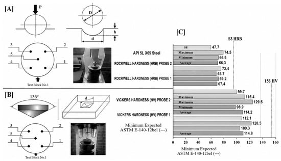
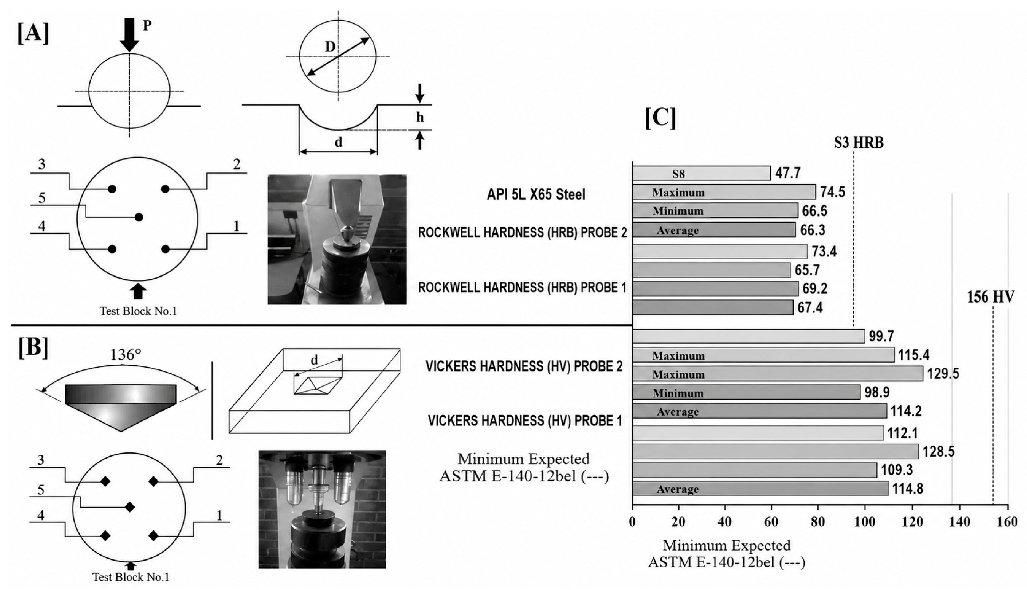
Vickers and Rockwell hardness measurements were performed on API L X65 steel according to ASTM E-92 and ASTM E-18 standards, using a 1/16′′ ball indenter with a load of 30 Kp for 15 s [27]. The results showed negative percentage differences of 26.9% and 19.8% relative to the reference values in ASTM E-140, indicating mechanical degradation of the material, as illustrated in Figure 14.

Figure 14. Rockwell and Vickers hardness tests. Results showing negative percentage differences of 26.9% Vickers (A) and 19.8% Rockwell (B) with respect to standard reference values. (C) Rockwell (HRB) and Vickers (HV) hardness test results for API 5L X65 steel.

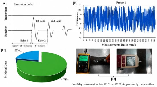
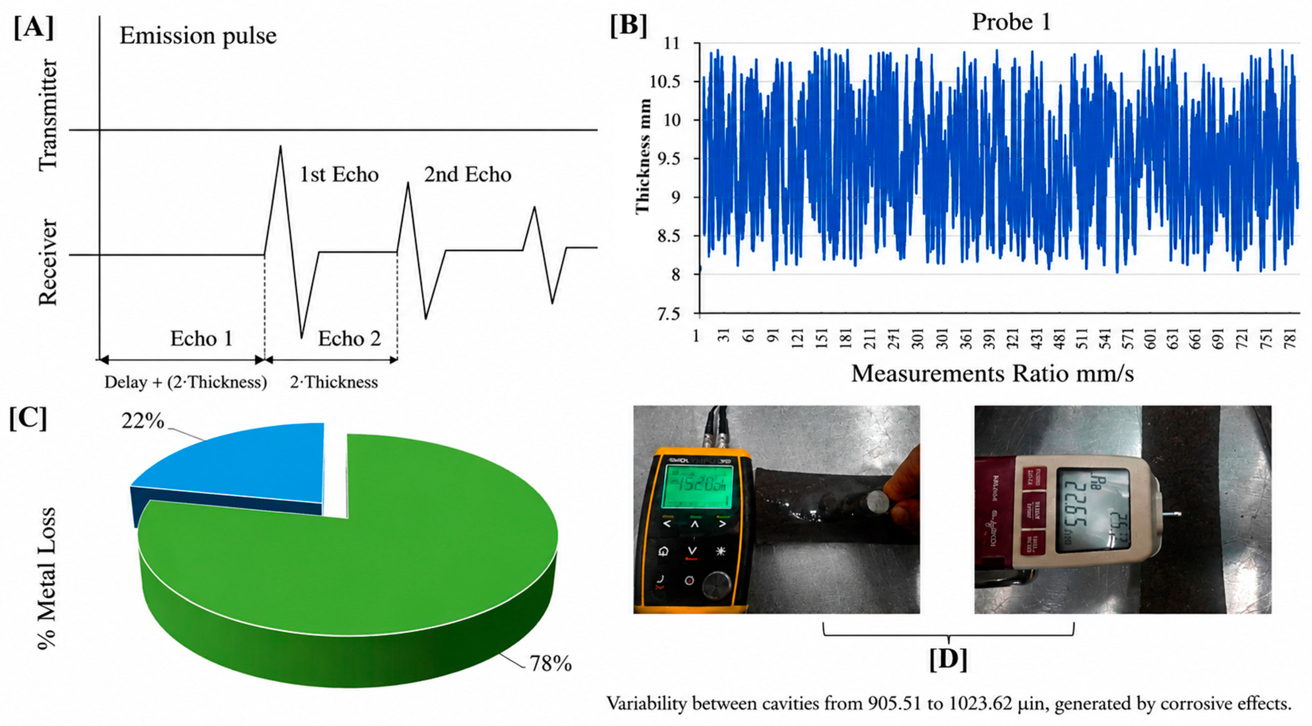
Ultrasonic thickness measurement is done by timing how long an acoustic wave takes to travel the distance. The operating principle is illustrated in image [A] of Figure 15. The experiment used a QS5 device with various probes (7.87″ and 1.96″), with a manufacturer-specified inter-layer thickness of 11 mm. The ultrasonic device maintains a nominal speed of 1.20 mm/second in longitudinal measurements.

Figure 15. Corrosion analysis by ultrasound and surface roughness. (A) Operating principle of ultrasonic thickness measurement; (B) ultrasonic measurement results for Probe 1; (C) metal loss indicators of 22%; (D) microgeometry of surfaces (cavity variability 905.51–1023.62 μin).

With a perimeter of 39.37″, 800 measurements were obtained showing variability caused by diverse cavities in the material from advanced corrosion. Figure 15 illustrates ultrasonic results for Probe 1 [B] and metal loss indicators of 22% [C] compared to manufacturer specifications. Length measurements defined the microgeometry of surfaces for each probe after structural fatigue, using a Mitutoyo SJ-201 profilometer, identifying cavity variability from 905.51 to 1023.62 micro-inches (μ in) caused by corrosive effects [D].

3.1.8. Design of the Tolerance Mechanisms of Subsystem 4

For subsystem 4, the data were divided and normalized, and the initial model architecture was defined. Goodness-of-fit tests and graphical analysis helped us to understand the behavior of input variables under adverse conditions. This was based on simulations of possible combinations of associated variables. Seven normalized variables within discrete ranges were represented by membership functions according to their behavior, along with five failure scenarios (See Table 10).

Table 10. Parameters for the linguistic variables of subsystem 4.

Variable (Inputs)	Linguistic Label	Membership Function	Interval
SYSSP—Specific yield strength of steel for a pipeline (MPa).	Minimum	1-Gamma	(0, 0.01, 449.99, 450.00)
	Average	Trapezoidal	(449.99, 450.01, 599.99, 600.00)
	Maximum	Gamma	(599.99, 600.01, 749.99, 750.00)
IPDF—Internal pressure established by the pipeline design factor (Kg/cm2).	Low	1-Gamma	(0, 0.01, 19.99, 20.00)
	Adequate	Trapezoidal	(19.99, 20.01, 59.99, 60.00)
	Reliable	Gamma	(59.99, 60.01, 80.50, 90.50)
GSSP—Grain size of steel for pipeline—ASTM E-112 (1:1).	Large	1-Gamma	(0, 0.01, 3.99, 4.00)
	Average	Trapezoidal	(3.99, 4.01, 10.99, 11.00)
	Small	Gamma	(10.99, 11.01, 13.99, 14.00)
FPPS—Ferrite–pearlite phase of pipeline steel (%).	Heterogeneous (high risk of fracture)	1-Gamma	(0, 0.01, 49.99, 50.00)
	Homogeneous (low risk of fracture)	Gamma	(49.99, 50.01, 99.99, 100.00)
PSG—Pipeline steel grade according to ASTM E8/E8M (MPa).	Minimum	1-Gamma	(0, 0.01, 534.99, 535.00)
	Average	Trapezoidal	(534.99, 535.01, 759.99, 760.00)
	Maximum	Gamma	(759.99, 760.01, 984.99, 985.00)
MCSH—Mechanical characterization of steel hardness using ASTM E-92, 18 and 140 (HRB).	Low hardness	1-Gamma	(0, 0.01, 50.99, 51.00)
	Average hardness	Trapezoidal	(50.99, 51.01, 85.99, 86.00)
	Maximum hardness	Gamma	(85.99, 86.01, 109.99, 110.00)
MCC—Alteration of the pipeline microstructure due to corrosive effects between cavities (μin).	Low	1-Gamma	(0, 0.01, 599.99, 660.00)
	Considerable	Trapezoidal	(599.99, 660.01, 1049.99, 1050.00)
	High	Gamma	(1049.99, 1050.01, 1599.99, 1600.00)
Variable (Outputs) Failure Scenarios
FS-22—Failure due to exceeding the specific elastic limit of the pipeline steel (%).	Minimal (low operational risk)	1-Gamma	(0, 0.1, 24.99, 25.00)
	Considerable	Trapezoidal	(24.99, 25.01, 74.99, 75.00)
	Critical (high risk of fracture)	Gamma	(74.99, 75.01, 99.99, 100.00)
FS-23—Failure due to exceeding the internal pressure established by the pipeline design factor (%).	Minimal (low operational risk)	1-Gamma	(0, 0.1, 19.99, 20.00)
	Considerable	Trapezoidal	(19.99, 20.01, 64.99, 65.00)
	Critical (high risk of fracture)	Gamma	(64.99, 65.01, 99.99, 100.00)
FS-24—Failure due to alteration in the grain size of the pipeline (%).	Minimal (low operational risk)	1-Gamma	(0, 0.1, 29.99, 30.00)
	Considerable	Trapezoidal	(29.99, 30.01, 64.99, 65.00)
	Critical (high risk of fracture)	Gamma	(64.99, 65.01, 99.99, 100.00)
FS-25—Failure due to alteration in the chemical composition of the pipeline material (%).	Minimal (low operational risk)	1-Gamma	(0, 0.1, 39.99, 40.00)
	Considerable	Trapezoidal	(39.99, 40.01, 79.99, 80.00)
	Critical (high risk of fracture)	Gamma	(79.99, 80.01, 99.99, 100.00)
FS-26—Failure due to alterations in the physical and elastic properties of the pipeline material (s/mm).	Low elongation time (high operational risk)	1-Gamma	(0, 0.1, 59.99, 60.00)
	Average elongation time	Trapezoidal	(59.99, 60.01, 95.99, 96.00)
	Desirable elongation time (minimum operational risk)	Gamma	(95.99, 96.01, 139.99, 140.00)
FS-27—Failure due to cracking and cavities in material thicknesses (%).	Minimal (low operational risk)	1-Gamma	(0, 0.1, 24.99, 25.00)
	Considerable	Trapezoidal	(24.99, 25.01, 59.99, 60.00)
	Critical (high risk of fracture)	Gamma	(59.99, 60.01, 99.99, 100.00)
FS-28—Failure due to micro-geometric alteration of pipeline material (%).	Minimal (low operational risk)	1-Gamma	(0, 0.1, 24.99, 25.00)
	Considerable	Trapezoidal	(24.99, 25.01, 59.99, 60.00)
	Critical (high risk of fracture)	Gamma	(59.99, 60.01, 99.99, 100.00)

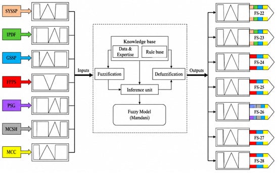
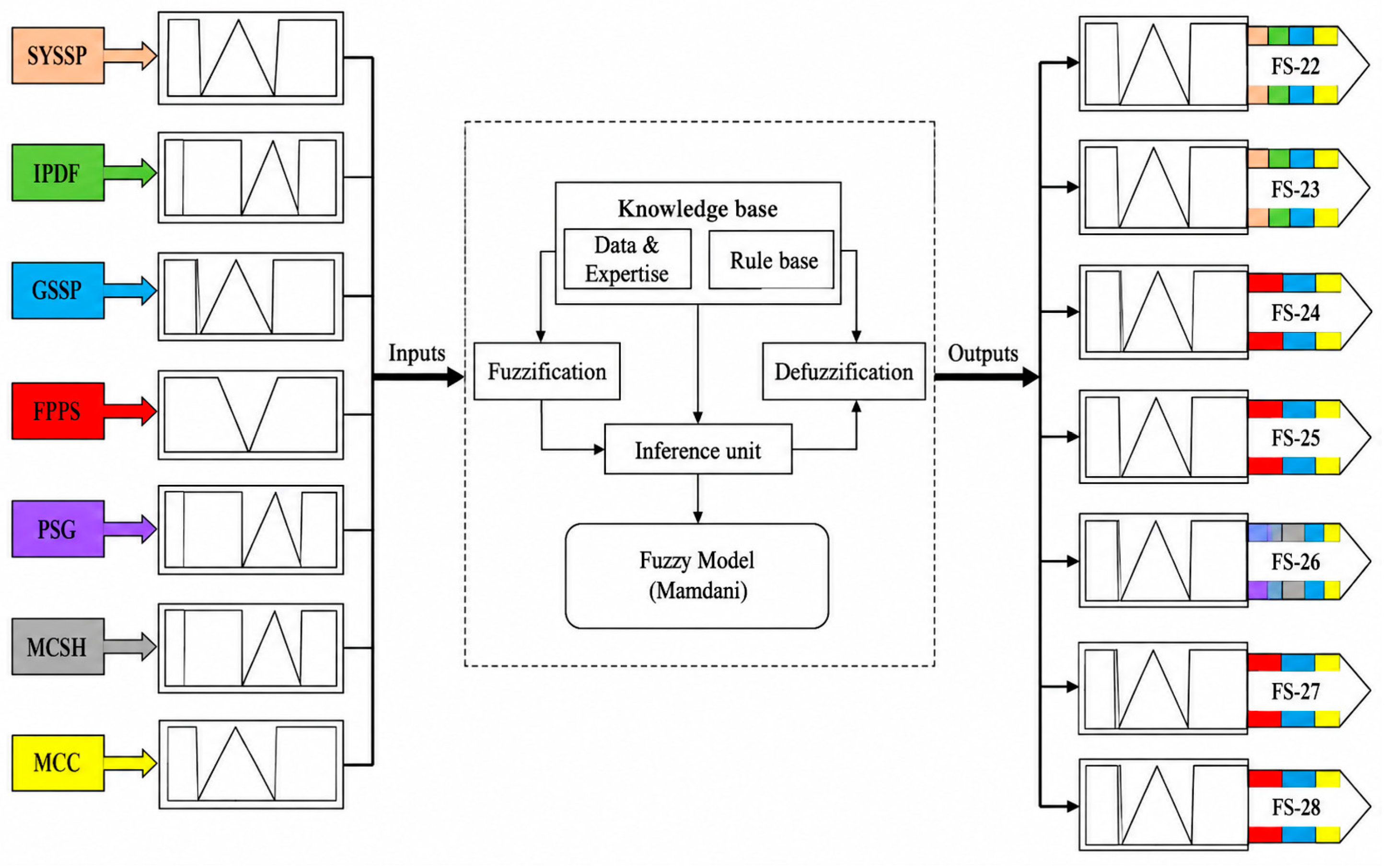
The fuzzy model interpreted a database with 354 metallographic observations, each described by seven input variables. This produced 2478 scalar measurements that were organized, normalized, and divided into training sets (1486 cases, 60%), validation sets (496 cases, 20%), and testing sets (496 cases, 20%). A total of 2187 inference rules were evaluated, corresponding to the Cartesian product of the linguistic categories assigned to the seven input variables. Sensitivity, consistency, and redundancy analyses identified rules with negligible activation and equivalent consequents. These rules were developed by consensus with 18 Level 1 and 2 certified technicians from Pemex Logístic and DTsi México. They specialize in AMPP standards, direct internal corrosion assessment (NACE SP0206-2006, NACE SP0208-2008) [15], cathodic protection systems, and the evaluation of coatings and corrosion inhibitors (NRF-005-Pemex-2007) [18]. Figure 16 presents the architecture of the fourth fuzzy system and the interaction between the input variables and the modeled failure scenarios.

Figure 16. Architecture of the fourth fuzzy model.

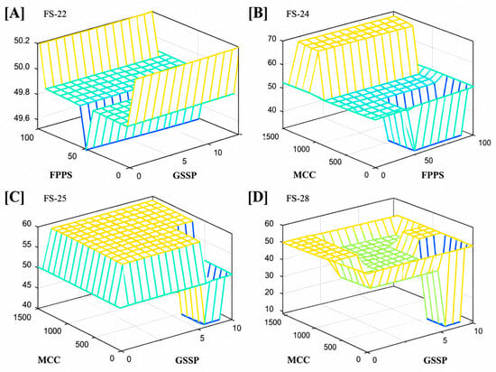
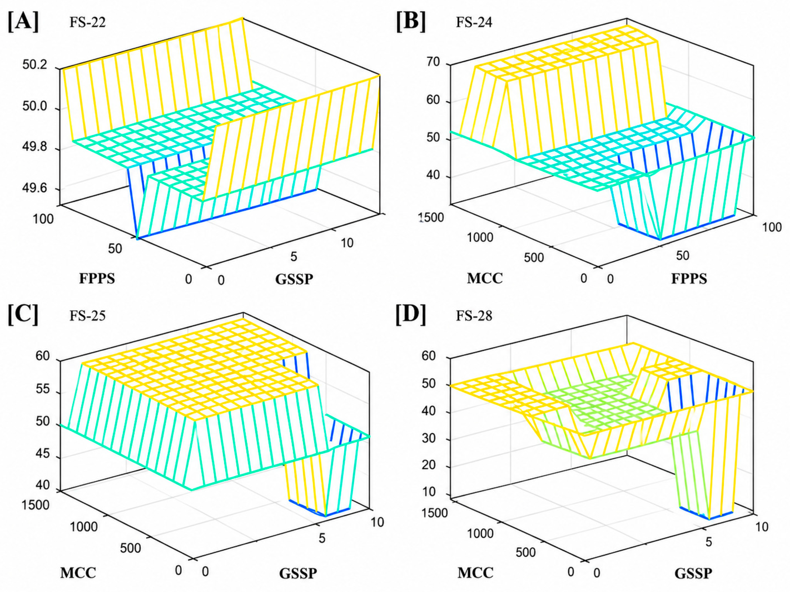
The reliability of subsystem 4 was validated using real-system data and fuzzy model estimates to identify variability in normalized outputs, similar to subsystem 1, with variance ranges between 1.02 and 3.90. The regression analysis showed strong agreement between experimental and predicted ỹ (t) = FS values, with an RMSE of 97.6%, MAE 95.9% and an adjusted R² of 95.1%. The standard error of the regression was 0.01759, indicating small deviations between predicted and observed values. Most observations were close to the regression line and within the 98.2% prediction interval. Figure 17 shows the response surface diagrams. Graph [A] FS-22 remains nearly constant around 50 across almost the entire domain. Its variation is small, suggesting the fault is activated or deactivated gradually as the FPPS and GSSP indicators change, indicating both variables have limited influence. [B] The activation of FS-24 shows three clearly differentiated regions. MCC has the greatest influence on its activation, while FPPS determines the minimum response zone. [C] FS-25 shows MCC predominates in triggering the fault, while GSSP mainly modulates it, decreasing to about 40% without significant impact. [D] FS-28 exhibits complex behavior with a wide response range. It has a central region of intermediate values near 30–45, surrounded by upper zones near 50–55. The surface geometry shows a pronounced nonlinear interaction: the effect of GSSP changes according to the MCC level, and vice versa.

Figure 17. Validation and comparison of the fuzzy model of subsystem 4; FS 22 = FPPS vs. GSSP (A); FS 24 = MCC vs. FPPS (B); FS 25 = MCC vs. GSSP (C); FS 28 = MCC vs. GSSP (D).

4. Design of the Diagnostic System

4.1. Detection, Isolation and Quantification of Failure Scenarios

Detecting faults in complex processes without available mathematical models is difficult; however, modeling and optimizing their behavior using AI is a prominent alternative today. Detecting fault scenarios allows for the diagnosis of nonlinear processes based on input/output data under normal operating conditions, enabling the quantification and isolation of faults in the system. This allows for the recovery of degraded operational phases through supervised reconfiguration.

The fault-signature matrix (FSM) is a tool used in the fault detection and isolation stage. Its function is to relate each possible system fault to the pattern of residuals, symptoms, or indicators expected when that fault occurs. Each row represents a residual, indicator, or symptom, and each column represents a possible fault.

$$\mathit{FSM}=\left[\begin{array}{ccc}{S}_{11}& \dots & S_{1m}\\ ⋮& \ddots & ⋮\\ S_{n1}& \dots & S_{\mathit{nm}}\end{array}\right]$$

(4)

where:

• R_i = residual or diagnostic indicator
• a_i = residual activation
• F_j = failure considered
• S_ij = expected response of the residual R_i to the failure F_j

S = |S_ij | ∈ {0,1}^mxn

(5)

$$S_{ij}=\left\{\begin{array}{c}1, \mathit{if} \mathit{residual} R_i \mathit{is} \mathit{activated} \mathit{by} \mathit{failure} F_j\\ 0, \mathit{The} \mathit{residual} \mathit{does} \mathit{not} \mathit{respond} \mathit{to} \mathit{the} \mathit{failure}\end{array}\right.$$

R_i (t) = y_i (t) − ŷ_i (t)

(6)

$${\mathit{a}}_{\mathit{i}}=\left\{\begin{array}{l}1, \left|{\mathit{R}}_{\mathit{i}}\right|>{\mathit{T}}_{\mathit{i}},\\ 0,\left|{\mathit{R}}_{\mathit{i}}\right|\le {\mathit{T}}_{\mathit{i}},\end{array}\right.$$

(7)

where:

• T_i = diagnostic threshold

This methodology, based on a set of consistency indicators called analytical redundancy relationships (ARRs) and high-gain dynamic state observers, was applied to reconstruct the evolution of the detected fault. These relationships are derived from the connections between the system elements (failure scenario).

For example:

If r¹, r³, r⁵, r⁷ ≠ 0 Then = FS-1

If r², r³, r⁶, r⁷ ≠ 0 Then = FS-2

The matrix contains, in coded form, the dependency of a given failure scenario (matrix column) on each residual (matrix row). Fault isolation consists of finding which of the fault signatures in the matrix most closely approximates the signature found experimentally. The diagnostic signature breadth used in this report is based on the count of residuals activated by each failure scenario out of a total of 28 possible, as shown in Table 11. The greater the number of activated residuals, the greater the propagation of the fault throughout the system and the more difficult its operational isolation becomes.

Table 11. Failure matrix of the pipeline.

	Failure Scenarios
Residuals		1	2	3	4	5	6	7	8	9	10	11	12	13	14	15	16	17	18	19	20	21	22	23	24	25	26	27	28
	1	1		1	1		1	1	1	1
	2		1	1	1	1		1	1	1
	3	1	1	1	1	1	1	1								1	1	1	1	1	1	1	1	1	1	1	1	1	1
	4			1	1	1	1	1		1	1	1	1	1	1	1	1	1	1	1	1	1	1	1	1	1	1	1	1
	5	1		1	1	1		1	1	1
	6		1	1	1		1	1	1	1
	7	1	1	1	1			1	1	1
	8			1	1				1	1
	9			1	1					1						1	1	1	1	1	1	1	1	1	1	1	1	1	1
	10			1	1					1	1	1	1	1	1
	11			1	1					1	1	1	1	1	1
	12			1	1				1	1	1	1	1	1	1
	13										1	1	1	1	1
	14										1	1	1	1	1
	15			1	1				1	1	1	1	1	1	1								1	1	1	1	1	1	1
	16			1	1				1	1	1	1	1	1	1	1	1						1	1	1	1	1	1	1
	17			1	1				1	1	1	1	1	1	1	1	1	1					1	1	1	1	1	1	1
	18			1	1				1	1	1	1	1	1	1	1	1	1	1				1	1	1	1	1	1	1
	19			1	1				1	1	1	1	1	1	1	1	1	1	1	1			1	1	1	1	1	1	1
	20			1	1				1	1	1	1	1	1	1	1	1	1	1	1	1		1	1	1	1	1	1	1
	21			1	1				1	1	1	1	1	1	1	1	1	1	1	1	1	1	1	1	1	1	1	1	1
	22			1	1				1	1	1	1	1	1	1	1	1	1	1	1	1	1	1	1	1	1	1	1	1
	23			1	1				1	1	1	1	1	1	1	1	1	1	1	1	1	1	1	1	1	1	1	1	1
	24			1	1				1	1	1	1	1	1	1	1	1	1	1	1	1	1	1	1	1	1	1	1	1
	25			1	1				1	1	1	1	1	1	1	1	1	1	1	1	1	1	1	1	1	1	1	1	1
	26			1	1				1	1	1	1	1	1	1	1	1	1	1	1	1	1	1	1	1	1	1	1	1
	27			1	1				1	1	1	1	1	1	1	1	1	1	1	1	1	1	1	1	1	1	1	1	1
	28			1	1				1	1	1	1	1	1	1	1	1	1	1	1	1	1	1	1	1	1	1	1	1

Table 12 presents the 28 scenarios ordered from highest to lowest number of activated residuals, with their assigned diagnostic signature breadth, and the fault matrix allows us to visualize that scenarios 3, 4, and 9 have a very close interaction with the entire system:

Table 12. Diagnostic signature breadth classification criteria.

[A]
Level	Activated Residuals	System Percentage	Operational Implication
Critical	24–28 residuals	≥86%	Affects practically the entire system. Difficult isolation.
High	18–23 residuals	64–82%	Wide propagation, requires priority intervention.
Medium	8–17 residuals	29–61%	Localized impact. Correctable with focused corrective action.
Low	1–7 residuals	≤25%	Fault contained and isolable. Low systemic impact.
[B]
Scenario	Description of Failure Scenarios	Subsystem	Residuals	Impact %	Diagnostic signature breadth
FS-3	Operational communication problem of the upstream or downstream station.	1	26	93%	Critical
FS-4	Failure due to exceeding the maximum safe operating pressure for a pipe with a metal loss indicator.	1	26	93%	Critical
FS-9	Leak due to mechanical deterioration (material fracture)	1	25	89%	Critical
FS-8	Leak at pipeline location (hydrocarbon theft)	1	21	75%	High
FS-10	Voltage rectifier failure, potential variability and electrical bridges	2	20	71%	High
FS-11	Failure in anode bed, anodes, cathodes, connections and conductors	2	20	71%	High
FS-12	Failure in mechanical pipeline coating	2	20	71%	High
FS-13	Failure due to corrosive aggressiveness of the soil	2	20	71%	High
FS-14	Failure due to corrosive soil resistivity	2	20	71%	High
FS-22	Failure due to exceeding the specific elastic limit of the pipeline steel	4	17	61%	Medium
FS-23	Failure due to exceeding the internal pressure established by the pipeline design factor	4	17	61%	Medium
FS-24	Failure due to alteration in the grain size of the pipeline	4	17	61%	Medium
FS-25	Failure due to alteration in the chemical composition of the pipeline material	4	17	61%	Medium
FS-26	Failure due to alterations in the physical and elastic properties of the pipeline material	4	17	61%	Medium
FS-27	Failure due to cracking and cavities in material thicknesses	4	17	61%	Medium
FS-28	Failure due to micro-geometric alteration of pipeline material	4	17	61%	Medium
FS-15	Failure by TIW (internal wall thickness of pipeline)	3	16	57%	Medium
FS-16	Failure by PTIW (wall thinning due to corrosion)	3	16	57%	Medium
FS-17	Failure by DIW (metal inclusions in internal wall)	3	15	54%	Medium
FS-18	Failure by LEIW (internal wall width of pipeline)	3	14	50%	Medium
FS-19	Failure by WALL (internal or external corrosive damage)	3	13	46%	Medium
FS-20	Failure by ERF (estimated pipeline repair factor)	3	12	42%	Medium
FS-21	Failure due to mechanical deterioration in a section of the pipeline	3	11	39%	Medium
FS-7	Failure in pipeline instrumentation and safety equipment	1	7	25%	Low
FS-1	Failure in dynamic equipment at upstream pumping station	1	4	14%	Low
FS-2	Failure in dynamic equipment at downstream pumping station	1	4	14%	Low
FS-5	Failure in upstream flow sensor or actuator	1	4	14%	Low
FS-6	Failure in downstream flow sensor or actuator	1	4	14%	Low

Diagnostic signature breadth represents the amplitude of the signature relative to interconnections with other subsystems, indicating diagnostic redundancy, potential propagation, and low isolation capability. However, greater residual activation does not necessarily mean greater physical damage. Conversely, a fault generating significant residuals can trigger multiple simultaneous faults, potentially causing the system to spiral out of control.

4.2. Key Findings

Scenario FS-3 is the only one that activates all 26 residuals, confirming the fault ma-trix observation that scenarios FS-3, FS-4, and FS-9 interact closely with the entire system. Both FS-3 and FS-4 belong to subsystem 1, which serves as a cross-cutting monitoring and control layer for all other subsystems. A failure in this subsystem compromises the overall diagnostic capability of the PTS.

The seven scenarios of subsystem 4 (FS-22–FS-28) exhibit a systemic impact through 17 activated residuals (61% of the system). Pipeline material properties (yield strength, composition, grain size, and microstructure) are fundamental conditions governing the behavior of all other subsystems. A metallurgical alteration propagates as a critical failure signature through the residuals in the matrix.

Structural scenarios FS-15–FS-21 exhibited progressively narrower signatures, decreasing from 16 to 11 activated residuals. This pattern suggests increasing diagnostic specificity rather than broader systemic propagation. Structural defects in the pipeline wall (TIW, PTIW, DIW, LEIW, WALL, ERF, and P Safe) are interrelated with each other and with variables in other subsystems as deterioration progresses. This makes late-stage failures significantly more difficult to isolate.

Localized failures are represented by low-impact scenarios such as FS-1, FS-2, FS-5, FS-6, and FS-7, which trigger between four and seven residuals, less than 25% of the failure matrix. Their failure signature is unique and well-defined, facilitating diagnostic isolation and reducing operational response time.

Implementing the diagnostic system allows early identification of failure scenarios by comparing observed and theoretical signatures. This is essential for modeling neuro-fuzzy tolerant control, which facilitates operational decision-making and activates specific tolerance mechanisms for each detected failure. It provides a robust tool for continuous monitoring and proactive management of pipeline integrity.

4.3. Limitations and Scope

This work is a new, comprehensive methodological contribution to monitoring and managing corrosion in a pipeline transport system through intelligent modeling of isolated parameters and variables that jointly influence the pipeline’s operational performance. However, its scope is limited by technical, operational, and contextual conditions to consider when interpreting results and planning implementation.

The system’s geographic and operational scope was developed and validated specifically for the Pemex Logística Nuevo Teapa-Tula pipeline (24″ and 30″ diameter, totaling 572 km), with emphasis on segments 9 and 8, covering 90 km along the Veracruz-Puebla border due to their high rates of vandalism.

The models were trained using historical data from 2010–2024, so their accuracy depends on the quality and continuous updating of databases in SAP and SCADA systems. Parameter recalibration is necessary when incorporating new data sources or extending to other sections of the national pipeline network.

The fuzzy logic-based tolerance mechanisms were built on the cognitive knowledge of specialists. While this adds to the system’s robustness, it creates dependence on the availability of expert personnel. The diagnostic system assumes a single failure, so scenarios with multiple simultaneous failures could exceed its current capacity. Ultrasonic inspection processed 4651 anomalies, identifying 12% as requiring priority attention with an ERF > 0.8. Detecting incipient failures in topographically difficult-to-access areas remains an operational challenge.

Although the system’s modular architecture facilitates adaptation to other industrial contexts, direct transfer to pipelines with metallurgical characteristics, hydrocarbon compositions, or geographic conditions substantially different from the studied pipeline requires a specific validation phase. The corrosive behavior models were built from Mexican crude oil blends—naphthenic, paraffinic, and asphaltic—which limits their applicability to hydrocarbons with significantly different physicochemical profiles.

The IMS was designed based on a predictive fault-tolerant control system with offline data, providing the foundation for online adaptive control. Currently, it is a decision-support tool that complements but does not replace the technical judgment of specialized personnel. Its gradual implementation through pilot sectors has trained new operating personnel in system reconfigurations during failures.

This article presents the first stage of the development and validation of the IMS; the second work will present the modeling, testing, and optimization of neuro-fuzzy control through the integration of genetic algorithms, as well as a cost–benefit analysis of the impact of failure scenarios through Monte Carlo simulation.

5. Discussion

The fault-signature matrix revealed a hierarchical pattern of failure propagation. Scenario FS-3 activated all 26 residuals. FS-4 and FS-9 also showed extensive interaction with other subsystems, confirming the transversal role of operational communication, pressure control, and monitoring functions. Metallurgical scenarios FS-22–FS-28 activated 17 residuals, or 61% of the matrix. Structural scenarios FS-15–FS-21 showed a decreasing from 16 to 11 activated residuals. In contrast, FS-1, FS-2, FS-5, FS-6, and FS-7 remained localized, activating fewer than 25% of the residuals and presenting more distinguishable signatures. These results indicate that diagnostic signature breadth depends not only on the initiating event but also on its capacity to propagate across operational, corrosion-protection, structural, and material domains.

The dominant signatures align with the physical mechanisms governing aged pipeline systems. Operational failures may reduce observability or cause pressure and flow deviations that promote hydraulic transients, cavitation, and cyclic stresses. At the same time, low soil resistivity, aggressive physicochemical conditions, coating degradation, and cathodic-protection deficiencies favor electrochemical dissolution and localized metal loss. This degradation appears in the progression of wall-thickness, corrosion-depth, defect-width, wall-loss, and estimated-repair-factor scenarios. At the material scale, changes in grain size, microstructure, mechanical properties, and defect population reduce the capacity of API L X65 steel to redistribute stresses, facilitating crack initiation and propagation. The matrix thus captures a coupled deterioration process where electrochemical damage alters structural resistance and operational loading accelerates defect evolution.

These findings complement international studies that have generally addressed corrosion prediction, structural integrity, or metallurgy as separate problems. BBN–GIS models have achieved high accuracy in predicting external corrosion depth. Probabilistic models validated against inline inspections have closely reproduced measured wall loss [15,18]. Likewise, metallurgical studies have shown the influence of microstructure, MnS inclusions, carbides, and corrosive environments on HIC, SSCC, and crack initiation in pipeline steels [16,17]. However, those approaches mainly provide condition or risk estimates without explicitly linking their outputs to system-wide fault propagation. The present results extend this knowledge by showing how operational, electrochemical, structural, and metallurgical anomalies interact within a unified diagnostic architecture. Nevertheless, direct performance superiority cannot yet be claimed because the present model and the cited approaches use different databases, outputs, and validation criteria.

A central contribution is the integration of historical SCADA, SAP, cathodic-protection, soil, ultrasonic-inspection, and metallurgical data with expert knowledge. Data-driven information anchors the rules in observed pipeline behavior. Specialist knowledge represents nonlinear interactions and rare but safety-critical events that may be underrepresented in historical databases. This hybrid construction improves interpretability because each diagnosis can be traced to activated variables, rules, and residuals, unlike purely black-box predictions. It also preserves operational knowledge accumulated by experienced personnel and converts heterogeneous information into comparable failure signatures. Consequently, the matrix provides more than a severity ranking. It establishes a structured basis for fault isolation, intervention prioritization, and subsequent fault-tolerant control.

From an operational perspective, widespread signatures such as FS-3, FS-4, FS-9, FS-8, and FS-10–FS-14 should receive priority because they may compromise both pipeline integrity and diagnostic capability. Localized signatures can support targeted maintenance. However, the results are limited to the studied 572 km network and depend on historical data quality, expert-defined membership functions, and the current single-fault assumption. Generalization requires recalibration and external validation in independent pipeline sections with different soils, coatings, operating regimes, and material histories. Future work should evaluate simultaneous and evolving failures, quantify diagnostic performance through sensitivity, specificity, F1-score, false-alarm rate, and detection delay, and prospectively validate the signatures using synchronized SCADA, CIPS, and inspection data. These steps will determine whether the proposed framework can reliably support online diagnosis and neuro-fuzzy reconfiguration under real operating conditions.

6. Conclusions

This study developed an interpretable fuzzy-logic framework integrating operational, cathodic-protection, mechanical-integrity, and metallurgical information from a 572 km aged pipeline network. Four Mamdani inference systems represented 28 failure scenarios through a unified fault-signature matrix. The models showed strong agreement with observed behavior, with adjusted (R²) values of 0.924, 0.946, 0.940, and 0.951 for the four subsystems.

The fault-signature matrix revealed clear differences in diagnostic propagation. FS-3 and FS-4 activated 26 of 28 residuals (93%), while FS-9 activated 25 (89%), showing critical system-wide influence. FS-10–FS-14 each activated 20 residuals (71%), and metallurgical scenarios FS-22–FS-28 activated 17 (61%). Structural scenarios FS-15–FS-21 decreased from 16 to 11 activated residuals (57–39%), while localized scenarios FS-1, FS-2, FS-5, FS-6, and FS-7 activated only four to seven residuals (14–25%), aiding fault isolation.

Overall, the framework provides a quantitative and interpretable basis for distinguishing localized from system-wide degradation, prioritizing maintenance, and supporting operator decision-making. Its applicability is limited to the analyzed network, historical data quality, expert-defined membership functions, and mainly single-failure scenarios. Future work should validate the framework under simultaneous and evolving failures and assess sensitivity, specificity, F1-score, false-alarm rate, and detection delay before implementing online neuro-fuzzy fault-tolerant control.

References

- Breton, T.; Sanchez-Gheno, J.C.; Alamilla, J.L.; Alvarez-Ramirez, J. Identification of failure type in corroded pipelines: A Bayesian probabilistic approach. J. Hazard. Mater. 2010, 179, 628–634. [Google Scholar] [CrossRef] [Scilit] [PubMed]
- Caleyo, F.; Alfonso, L.; Espina-Hernández, J.H.; Hallen, J.M. Criteria for performance assessment and calibration of in-line inspections of oil and gas pipelines. Meas. Sci. Technol. 2007, 18, 1787–1799. [Google Scholar] [CrossRef] [Scilit]
- Canavese, G.; Scaltrito, L.; Ferrero, S.; Pirri, C.F.; Cocuzza, M.; Pirola, M.; Corbellini, S.; Ghione, G.; Ramella, C.; Verga, F.; et al. A novel smart caliper foam pig for low-cost pipeline inspection-Part A: Design and laboratory characterization. J. Pet. Sci. Eng. 2015, 127, 311–317. [Google Scholar] [CrossRef] [Scilit]
- Braswell, G. Artificial Intelligence Comes of Age in Oil and Gas. J. Pet. Technol. 2013, 65, 50–57. [Google Scholar] [CrossRef] [Scilit]
- Lin Cao, A.; Jun Zhu, Q.; Tao Zhang, S.; Rong Hou, B. BP neural network predictive model for stray current density of a buried metallic pipeline. Anti-Corros. Methods Mater. 2010, 57, 234–237. [Google Scholar] [CrossRef] [Scilit]
- Cai, B.; Liu, Y.; Liu, Z.; Tian, X.; Zhang, Y.; Ji, R. Application of bayesian networks in quantitative risk assessment of subsea blowout preventer operations. Risk Anal. 2013, 33, 1293–1311. [Google Scholar] [CrossRef] [Scilit] [PubMed]
- Castellanos, V.; Albiter, A.; Hernández, P.; Barrera, G. Failure analysis expert system for onshore pipelines. Part-I: Structured database and knowledge acquisition. Expert Syst. Appl. 2011, 38, 11085–11090. [Google Scholar] [CrossRef] [Scilit]
- Canyurt, O.E.; Ozturk, H.K. Application of genetic algorithm (GA) technique on demand estimation of fossil fuels in Turkey. Energy Policy 2008, 36, 2562–2569. [Google Scholar] [CrossRef] [Scilit]
- Velázquez, J.C.; Valor, A.; Caleyo, F. Statistical study of localized internal corrosion defects in oil and gas pipelines through sampling inspection. Process Saf. Environ. Prot. 2024, 186, 566–576. [Google Scholar] [CrossRef] [Scilit]
- Xu, Y.; Zheng, C.; Yi, G.; Ma, H.; Ju, D.; Zhang, J.; Hu, X. Sensitivity to hydrogen induced cracking, and corrosion performance of an X65MS pipeline steel in H2S containing environment. J. Pipeline Sci. Eng. 2026, 6, 100280. [Google Scholar] [CrossRef] [Scilit]
- Quispe-Avilés, J.M.; Imata-Condori, R.; Mamani-Quiñones, G.A.; Canahua-Loza, H.; Gonzales-Condori, E.G.; Ariza-Echeverri, E.A. Analysis of cracks caused by hydrogen damage in HSLA X70 in sour gas media using conventional and non-destructive techniques. Gas Sci. Eng. 2026, 145, 205778. [Google Scholar] [CrossRef] [Scilit]
- Cid-Galiot, J.J.; Aguilar-Lasserre, A.A.; Rodriguez-Jarquín, J.P.; Villanueva-Vasquez, D.; Posada-Gómez, R.; Juárez-Martínez, U. Fault-Tolerance Techniques and Global Positioning Systems Based on Artificial Intelligence for the Analysis of Corrosion Impact on the Pipelines of Oil and Gas Industry. J. Press. Vessel Technol. 2021, 143, 020801. [Google Scholar] [CrossRef] [Scilit]
- Pemex. Procedimiento Para la Operación de la Estación de Rebombeo No. 5 ‘A’ Mendoza Oleoducto 24″–30″ Ø Nuevo Teapa–Venta de Carpio–Tula-Salamanca 583-51540-PEO-04.pdf; Pemex: Mendoza, Veracruz, Mexico, 2012. [Google Scholar]
- NRF-047-PEMEX-2007; Diseño, Instalación Y Mantenimiento de los Sistemas de Protección Catódica. Comité de Normalización de Petróleos Mexicanos y Organismos Subsidiarios: México City, Mexico, 2007.
- Kulikov, V.P.D.; Khodak, M.; Efimov, M. Reporte Final UHR-Oleoducto 30″ D.N., Cd. Mendoza-Venta de Carpio, Sección: Cd. Mendoza-Maltrata, 9.7 km; Weatherford: Ciudad Mendoza, Veracruz, Mexico, 2011. [Google Scholar]
- ASME B31G; Manual for Determining the Remaining Strength of Corroded Pipelines Supplement to ASME B31 Code for Manual for Determining the Remaining Strength of Corroded Pipelines. ASME: New York, NY, USA, 1991.
- Pemex. Petróleos Mexicanos; Pemex: Mendoza, Veracruz, Mexico, 2020; pp. 1–98. [Google Scholar]
- Refinación, P. FILOSOFÍA OPERATIVA DEL OLEODUCTO NUEVO TEAPA-VENTA DE CARPIO-TULA-SALAMANCA 24″ 30″; Pemex: Mendoza, Veracruz, Mexico, 2011; Available online: https://www.pemex.com (accessed on 19 May 2026).
- Dtsi. Reporte de Estudio CIPS Realizado al Oleoducto 24″ Ø Nuevo Teapa–Tula PXR-OP-SCC-SUD-GCM-L-13-14; Dtsi: Mendoza, Veracruz, Mexico, 2016. [Google Scholar]
- Vieira, R.E.; Kesana, N.R.; Shirazi, S.A.; McLaury, B.S. Experiments for sand erosion model improvement for elbows in gas production, low-liquid loading and annular flow conditions. In Proceedings of the CORROSION 2014, San Antonio, TX, USA, 9–13 March 2014. [Google Scholar]
- ASTM E112-13; Standard Test Methods for Determining Average Grain Size. ASTM International: West Conshohocken, PA, USA, 2013; pp. 1–28.
- ASTM E18−16; Standard Test Methods for Rockwell Hardness of Metallic Materials. ASTM International: West Conshohocken, PA, USA, 2016; pp. 1–38.
- ASTM G1-90; Standard Practice for Preparing, Cleaning, and Evaluating Corrosion Test Specimens. ASTM International: West Conshohocken, PA, USA, 1999.
- ASTM E140-12b; Standard Hardness Conversion Tables for Metals Relationship Among Brinell Hardness, Vickers Hardness, Rockwell Hardness, Superficial Hardness, Knoop Hardness, Scleroscope Hardness, and Leeb Hardness. ASTM International: West Conshohocken, PA, USA, 2012. [CrossRef] [Scilit]
- ASTM E112-96; Standard Test Methods for Determining Average Grain Size. ASTM International: West Conshohocken, PA, USA, 2004; pp. 1–26. Available online: https://store.astm.org/e0112-25.html (accessed on 26 May 2026).
- ASTM E8; ASTM E8/E8M Standard Test Methods for Tension Testing of Metallic Materials; ASTM International. West Conshohocken, PA, USA, 2010.
- Bassam, A.; Ortega-Toledo, D.; Hernandez, J.A.; Gonzalez-Rodriguez, J.G.; Uruchurtu, J. Artificial neural network for the evaluation of CO2 corrosion in a pipeline steel. J. Solid State Electrochem. 2009, 13, 773–780. [Google Scholar] [CrossRef] [Scilit]
Disclaimer/Publisher’s Note: The statements, opinions and data contained in all publications are solely those of the individual author(s) and contributor(s) and not of MDPI and/or the editor(s). MDPI and/or the editor(s) disclaim responsibility for any injury to people or property resulting from any ideas, methods, instructions or products referred to in the content. |
© 2026 by the authors. Licensee MDPI, Basel, Switzerland. This article is an open access article distributed under the terms and conditions of the Creative Commons Attribution (CC BY) license.