


Abstract
Airborne laser scanning (ALS) and UAV-mounted LiDAR sensors have become well-established tools for identifying and mapping archaeological features across varying scales and contexts. Numerous algorithms have been developed over the years for generating Digital Terrain or Features Models (DTMs/DFMs), which provide an accurate representation of the ground or structures’ surface, serving as the foundation for subsequent archaeological analyses. In this study, we report the developed multi-level multi-resolution (MLMR) methodology, based on machine/deep learning methods, for DFM generation through point cloud semantic segmentation. The work also compares different approaches and the impact of the resolution on their performance. To this end, each approach’s performance is evaluated with a series of quantitative and qualitative analyses, with an eye on hardware limitations and time constraints. Three test sites from Mediterranean and Alpine environments, with manually annotated ground truth data, are used for the evaluation of each methodological approach.
1. Introduction
Airborne laser scanning (ALS) and unmanned aerial vehicle (UAV)-mounted light detection and ranging (LiDAR) sensors have become well-established tools for identifying and mapping archaeological features at varying scales and in diverse contexts. Their ability to penetrate forest canopy enables archaeologists to detect otherwise invisible structures [1,2,3,4]. As these technologies have become more accessible and point densities have increased, the resulting data volumes have grown substantially, necessitating effective automated methods for extracting meaningful archaeological information from point clouds.
To this end, numerous algorithms have been developed over the years to generate digital terrain models (DTMs), which provide an accurate representation of the ground surface and serve as the foundation for subsequent archaeological analysis. DTM analysis represents a crucial step in archaeological LiDAR workflows, enabling the detection of potential archaeological anomalies in under-canopy areas that would otherwise remain invisible in aerial imagery.
By design, a DTM is a representation of the bare-earth surface, free of any other objects standing on it, such as buildings, vegetation, or cars. However, an archaeological DTM has specific requirements that differ from a standard DTM. For comprehensive detection of archaeological features, a DTM needs to be free of vegetation, but structures, standing walls, roads, channels, earthworks, and any other standing archaeological features should survive any filtering and be represented in the final model. This archaeology-specific elevation model has been defined as an “archaeological digital elevation model” or called Digital Feature Model (DFM) [5]. This concept has recently gained interest, and several archaeology-specific pipelines have been proposed for its generation and use [6,7,8].
However, DTM/DFM generation is a complex procedure requiring numerous assumptions and decisions, starting from the project planning, where data acquisition parameters (flight height, pulse density, etc.), seasonal conditions, terrain slope, and forest characteristics must be considered, to the choice of analytical workflow for processing, where numerous steps along the processing workflow can heavily influence the final output [9,10].
While multiple operations influence the final DFM outcome, including raster interpolation methods, point cloud ground filtering represents one of the most critical steps, as it directly affects the archaeological interpretability of the data. In this context, traditional filters are not designed to retain standing archaeological features, and challenging conditions such as abrupt elevation changes, dense forest, or shrubbery cover hamper their ability to extract an accurate ground surface with fixed settings. In such cases, manual point cloud segmentation is often required to prevent loss of archaeological information during filtering. This is an extremely time-consuming procedure that becomes unfeasible at a large scale in densely forested areas.
In that sense, machine learning (ML) approaches for semantic segmentation, which learn discriminative patterns directly from labelled examples, can be trained to retain both ground and archaeological features in the final output, avoiding extensive adaptive strategies and parameter tuning, and offering a viable and more flexible alternative to traditional filtering, especially in complex, densely forested, and mixed environments.
To this end, inspired by previous approaches applied to the heritage domain [11,12], a multi-level multi-resolution (MLMR) framework was proposed for archaeological point cloud semantic segmentation, employing Random Forest (RF) [13] or Point Transformer (PT) [14] as pipeline backbone [8,15].
The MLMR methodology applies a modular approach to point cloud semantic segmentation, subdividing the task into two specialised steps. At first, it extracts a DFM at a coarser level (L1), then maps archaeological above-ground features at a finer level of granularity (L2).
Building upon our prior work [8,15], this study revises the MLMR methodology by introducing a train–test consistency strategy to train the pipeline’s second level on data that more closely resembles the real L1 output rather than ideal ground truth (GT).
The innovative aspects of the proposed method are:
- The use of a train–test consistency strategy for L2 training inside the MLMR framework.
- The removal of any manual correction procedure between the two levels of the methodology.
To evaluate the performance of the proposed pipeline, controlled comparisons across three test sites in Mediterranean and Alpine environments are conducted at different resolutions. We compare:
- MLMR methodology with RF vs. PT backbones.
- Hierarchical MLMR methodology vs. a segmentation approach in which all classes are predicted in a single stage (from now on referred to as “end-to-end” approach).
Each experimental comparison is analysed using quantitative methods, with standard ML metrics calculated and compared against a manually annotated GT, and qualitative comparisons by visual inspection of the results.
Following the literature review presented in Section 2, Section 3 presents the experimental setup; Section 4 presents the results with quantitative comparisons; and Section 5 provides a discussion, including a qualitative analysis. Finally, Section 6 presents conclusions, current limitations, and future research directions.
2. Related Works
Since the early 2000s, the analysis of topographic surfaces derived from LiDAR has significantly impacted the study and documentation of archaeological landscapes, becoming an invaluable source of information for archaeologists worldwide. Following pioneering archaeological applications in Germany and the United Kingdom [16,17,18,19], the number of archaeological studies utilising LiDAR has increased steadily and its usage has expanded to Europe, North America, Central America, and Southeast Asia, with over 200 studies demonstrating the technology’s fundamental role in landscape understanding [4].
LiDAR has proven particularly successful in heavily forested environments, where its ability to penetrate the canopy enables archaeologists to reveal landscapes otherwise invisible to aerial photography and even field surveys, where limited spatial perspective, reduced ground visibility, and subtle topographic relief make the detection of archaeological features very challenging.
2.1. LiDAR Applications in Archaeology
Geographically, most archaeological LiDAR studies have been conducted in Europe and the Americas; outside these two regions, Southeast Asia stands out as an exception, with extensive surveys in Cambodia. Within this global distribution, tropical and subtropical environments yield the most remarkable results, with numerous studies revealing complex urbanised landscapes concealed by dense vegetation [20,21,22], including valuable contributions from local scholars [23].
In recent years, the application of ALS to archaeology has yielded some of its most spectacular results in Mesoamerica, revolutionising Maya archaeology. Entire archaeological landscapes, with complex settlements and imposing structures, have been discovered in the Maya lowlands, significantly impacting the understanding of Maya settlement patterns and territorial organisation [22,24,25,26]. The landmark study by Canuto et al. [21], analysing LiDAR data covering more than 2000 km2 of lowland Guatemala and identifying more than 60,000 archaeological features, exemplifies the magnitude of the technology’s impact; an impact further demonstrated by subsequent studies revealing new evidence of regional spatial settlement patterns and organisation in Maya society [27,28]. Similarly, in Southeast Asia, LiDAR surveys have uncovered previously concealed urban networks beneath dense forest canopy, most notably around the Angkor Wat complex in Cambodia [20,29,30,31], confirming LiDAR’s role as a key technology for archaeology in tropical environments.
In stark contrast to Mesoamerica and Southeast Asia, where standing features ranging from several metres to tens of metres in height are not uncommon, European archaeological features exhibit limited vertical relief and are mostly embedded in the ground. Consequently, European studies employ LiDAR mostly to analyse topography, where even subtle variations, often associated with anthropogenic activity, can aid in detecting and mapping archaeological features. In Europe, the use of LiDAR data in archaeology is unevenly distributed, and it is typically correlated with the availability of open data provided by public agencies, with Italy [32,33,34,35], the United Kingdom [36,37,38], and Spain [39,40,41] producing the largest number of studies (4).
While publicly available data facilitates the widespread adoption of this technology in archaeology, with large projects documenting archaeological features at vast scales [39,42,43,44], recent high-resolution acquisition campaigns for archaeological purposes enable higher levels of detail in landscape analysis [7,10]. Specifically, the development of full-waveform LiDAR sensors [45] and their recent integration with UAVs enable the acquisition of high-resolution datasets, reaching point densities of hundreds of points per square metre, significantly increasing the level of detail achievable in archaeological analysis [8,15].
2.2. Archaeological LiDAR Data Processing
While its widespread application and impact in archaeology are clear and uncontested, LiDAR use in archaeology requires careful consideration.
A LiDAR workflow requires great care at each step, beginning from the planning phase, where particular attention must be given to vegetation cover, as it influences pulse penetration and, consequently, the quality of the resulting DFM. Several studies examine how different vegetation types affect the detectability of archaeological features [46,47,48], though the influence of acquisition date in relation to the vegetative cycle remains largely unexplored, with Doneus et al. [7] representing, to our knowledge, the only study to examine this temporal aspect in depth. Following the planning phase, several processing steps (system calibration, data acquisition, georeferencing, flight strip adjustment, and registration) are required to generate the final point cloud, each influencing its quality [10]. However, after point cloud registration, three processing stages are particularly critical for the detectability of archaeological features: point cloud classification/filtering, DTM/DFM interpolation, and visualisation.
Many studies over the past 20 years have focused on the latter, employing different visualisation techniques (VTs) such as hillshade, slope, sky view factor, and openness to improve the visibility of archaeological features [49,50,51], proving to be highly effective for the analysis of archaeological landscapes. However, VTs alone do not address the limitations of traditional manual prospection and interpretation approaches for processing large datasets [52], which are becoming increasingly evident as data volumes continue to grow. To this end, automated workflows that combine DTMs/DFMs with a variety of visualisation techniques to detect archaeological features have been developed over the years. From pipelines using algorithms such as template-matching, automated feature extraction, and object-based image analysis (OBIA) [53,54], the field has progressively shifted toward ML algorithms, with the studies of Guyot et al. [55] and Niculiță [56], where the RF algorithm is employed to identify burial mounds, exemplifying this shift. More recently, however, the rapid advancement of deep learning (DL) neural networks largely supplanted these standard ML approaches. The studies of Trier et al. [57] and Verschoof-van der Vaart and Lambers [58] use R-CNNs (Regions-based Convolutional Neural Networks) for the automated detection of multiple classes of archaeological objects in LiDAR data in Norway and in the Netherlands, while Berganzo-Besga et al. [59] combine multi-scale relief model visualisation with YOLOv3, an R-CNN-based DL algorithm, to perform DTM-based shape detection of archaeological tumuli with high accuracy, demonstrating the potential of this technology in the field.
While VTs have long been the subject of scholarly attention in the field, archaeological-specific interpolation methods for DTM/DFM generation are considered only briefly in a handful of studies [10,60]. The lack of archaeological interest can be attributed to two main reasons: first, the notion that visualisation techniques and classification/ground-point filtering are the main factors influencing the detectability of archaeological features; second, the reliance of most archaeological pipelines for LiDAR data processing on black-box approaches.
Despite this lack of attention, interpolation is an important factor in DFM generation, significantly impacting the visibility of archaeological features, as off-terrain structures such as earthworks and walls are highly sensitive to interpolation artefacts and smoothing. Few studies compare different interpolators specifically for archaeological applications. Triangulation with linear interpolation (TLI) is considered the most suitable for LiDAR dense point clouds in a study by De Boer et al. [61], due to its limited smoothing effect, while recent studies [62,63] advocate Kriging as the better option, especially at low point densities. The comprehensive study by Štular et al. [60] delves deeper into the topic and compares six interpolators available from free or low-cost software on four test sites in Europe, all presenting challenging conditions such as sharp discontinuities and vegetation on steep slopes, concluding that no interpolator is clearly the best on all occasions and that hybrid interpolators can achieve the best results.
However, before the final stages of interpolation and visualisation can be undertaken, point cloud ground filtering/segmentation is required to separate DFM points from unwanted data. This step is among the most critical stages in the processing workflow because it directly determines which and how many archaeological features are retained in the final DFM [10]. To this end, many ground filtering algorithms have been developed over the years, ranging from triangulated irregular networks [64] to progressive morphological filters [65] to more recent cloth-simulation approaches [66].
In a standard archaeological LiDAR processing workflow, domain experts typically use existing ground filtering algorithms available in open-source and/or proprietary software and, in some cases, refine the results with manual filtering operations. This operation is conducted using various software packages, both commercial (LAStools1, TerraScan2) and open-source (PDAL3, CloudCompare4), with comparative assessments available in the general remote sensing literature [67,68] and archaeological-specific reviews [37,69].
A recent study by Doneus et al. [10] examines ground filtering in challenging Mediterranean environments, revealing significant parameter sensitivity across diverse archaeological sites. Filtering involves a fundamental trade-off: aggressive filtering removes vegetation but risks losing archaeological features, while conservative filtering preserves structures but retains vegetation noise. This compromise is manageable in deciduous forests with sparse undergrowth, but densely vegetated evergreen environments pose greater challenges, particularly when combined with highly variable topography where fixed-parameter approaches fail. Recognising these context-dependent challenges, Doneus et al. [70] developed a spatially adaptive filtering pipeline in which expert users test multiple algorithms on sample areas through an accessible interface, selecting optimal approaches for each zone, while preserving a human-in-the-loop methodology to leverage domain knowledge alongside computational tools.
Štular and Lozić [69] compare available ground filtering algorithms, finding that all filters struggle with extreme vegetation conditions and steep slopes, and, surprisingly, that older, established filters often outperform newer ones. A key finding of the study is that, although most filters retain fully embedded and, to a lesser extent, partially embedded archaeological features, none fully preserve standing structures because ground filters, by design, filter out non-terrain objects. Consequently, retaining standing features requires considerable manual classification effort.
To fill this gap, ML methods may offer a viable, more flexible alternative to traditional algorithms in diverse, densely vegetated environments, enabling the detection and classification of archaeological features that traditional algorithms struggle to distinguish. This is particularly relevant for tropical and subtropical environments (e.g., Mesoamerica, Southeast Asia), where large datasets comprising numerous above-ground archaeological structures may benefit greatly from this approach, as well as for temperate and Mediterranean forests in Europe, where subtle, low-relief features can be confused with natural terrain. However, direct application of ML/DL approaches to 3D archaeological point clouds remains rare. To the best of our knowledge, Richards-Rissetto et al. [71] represent the first application in the field, employing the PointConv architecture for feature detection on archaeological point clouds. However, their study performs region-level detection rather than point-level semantic segmentation, leaving point-level semantic segmentation for Digital Feature Model (DFM) generation largely unexplored.
3. Methodology
This section presents the MLMR methodology, including the newly introduced sequential training–test consistency strategy, in which L2 is trained on L1’s predicted outputs rather than GT labels. Following the hierarchical framework description, we detail the datasets used in the experiments, the employed algorithms/architectures, the training setup, and the metrics used to evaluate the results.
3.1. Multi-Level Multi-Resolution Approach (MLMR)
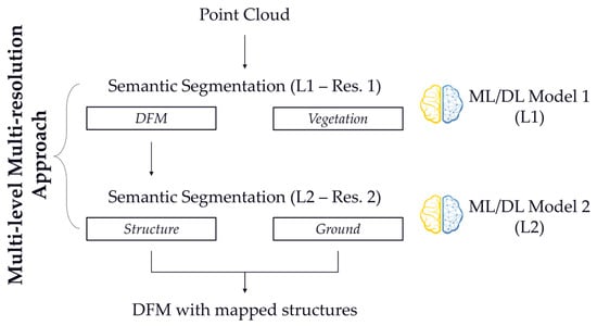
The MLMR approach (Figure 1) is a hierarchical framework comprising two consecutive binary semantic segmentation stages performed progressively from coarser to finer resolution. This design reduces computational overhead by processing full-resolution data only at the final stage, shortens training times, and enables task-specific optimisation at each stage, maintaining fine-scale accuracy while improving computational efficiency. The semantic segmentation task is decomposed into two stages:
Figure 1.
The MLMR approach scheme.
- Level 1 (L1)—Vegetation Filtering: At the first level, the model is trained on GT labels to distinguish vegetation from non-vegetation at a lower resolution. This progressive filtering substantially reduces the dataset from its original size (76% reduction in the tested datasets) before the more challenging structure detection stage, improving the effective class ratio for structures among the remaining points (from ~3% to ~12% in the tested datasets) and substantially alleviating the class imbalance for the critical second stage.
- Level 2 (L2)—Structure Detection: After reprojecting L1’s predictions to a finer resolution and filtering out the predicted vegetation, at the second level, the ML algorithm is trained to distinguish structures from ground. L2 is trained on L1’s predicted labels applied to training and validation sets rather than GT. Inspired by cascade architectures in object detection [72], this train–test consistency strategy addresses the distributional mismatch problem. During inference, L2 receives L1’s imperfect predictions, making training on L1’s outputs more representative of deployment conditions than training on GT.
The MLMR hierarchy employed in this study builds upon previous implementations while introducing key refinements. We adopt a vegetation-first approach from Mazzacca et al. [15], minimising error propagation, leveraging vegetation’s distinctive geometric signature (high vertical extent and anisotropy) to perform the simpler binary task first and enabling fully automatic inference without manual correction between pipeline stages. However, we introduce a novel training strategy, unlike prior work [8,15], in which both levels are trained on GT labels. In this study, L2 training is performed on L1’s predictions to improve robustness against upstream errors.
3.2. Class Selection
Following previous studies [8,15] and the typical needs of archaeologists when processing LiDAR data over under-canopy heritage sites, the proposed pipeline is built around the segmentation of three classes (structure, vegetation, and ground), with the classes ground and structure functioning as the basis for the DFM generation.
Although a DFM, by definition, contains only archaeological structures (excluding modern ones), in this study, modern and archaeological structures are grouped together inside the structure class for several reasons:
- The need to avoid potential loss of archaeological features by adding further complexity to the segmentation task, particularly given that the structure class, in general, is already severely underrepresented in archaeological LiDAR datasets.
- The inherent difficulty of defining this distinction in geometric terms, as it requires stylistic-interpretative considerations and conservation state assessments, is that it cannot be readily translated into neural network training parameters.
- The scarcity of modern structures in forested environments, which, in conjunction with the previous two points, considerably limits the advantages of an automated approach compared to manual expert assessment.
3.3. Datasets
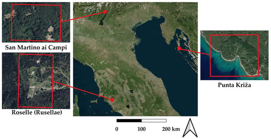
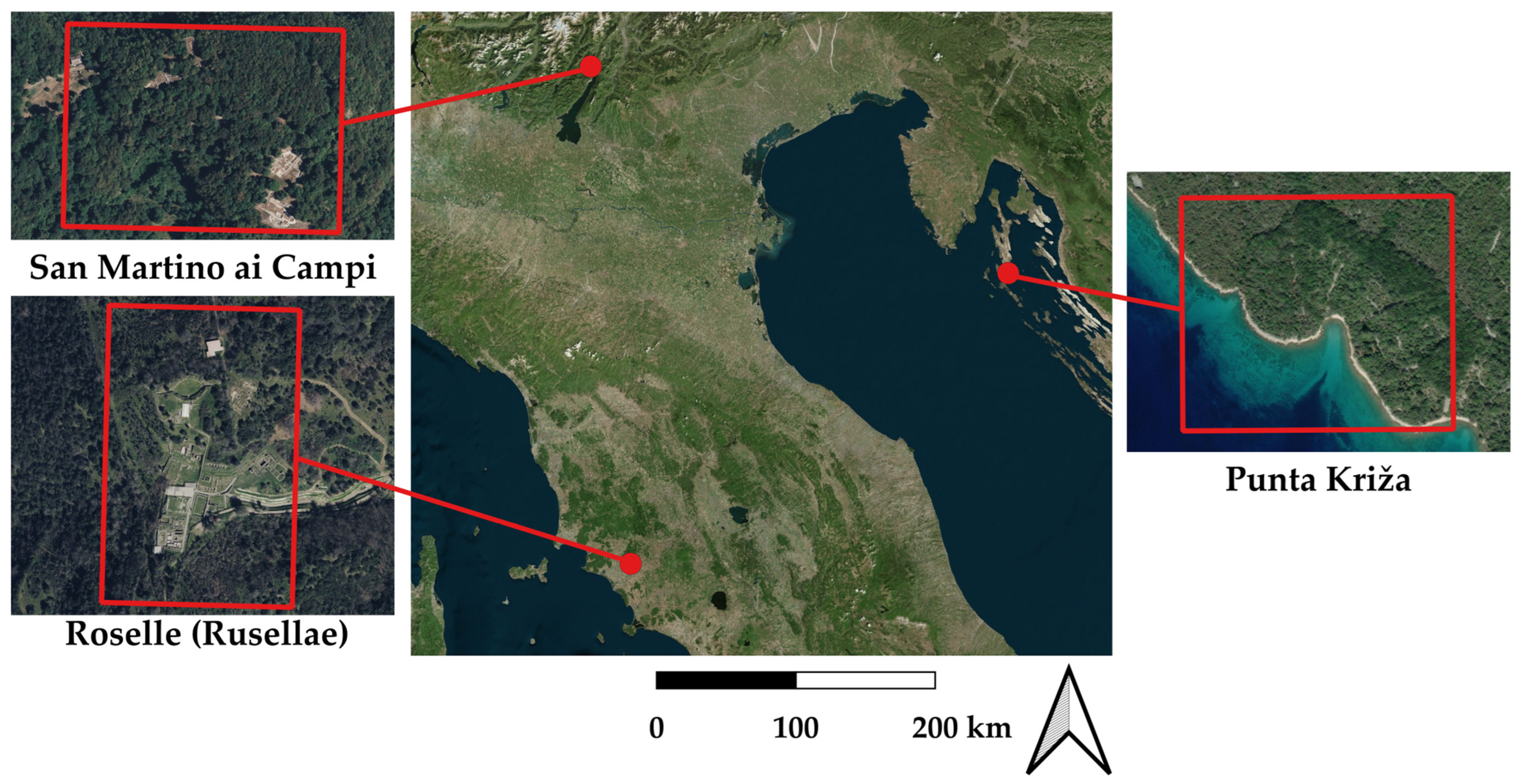
Three datasets are used in the experiments (Figure 2), acquired with different aerial sensors, platforms, and pulse densities (Table 1) over archaeological contexts with distinct geomorphological settings and varying vegetation types and densities (Table 2). Each dataset is annotated into the three selected classes (structure, vegetation, ground) by domain experts, with annotations validated through published studies [8,15,73,74].
Figure 2.
Locations of the study areas used in this paper and close-view panels illustrating the extent of the areas (© Microsoft Bing Maps).
Table 1.
Datasets acquisition characteristics.
Table 2.
Characteristics of the datasets.
3.3.1. Dataset 1: San Martino ai Campi
A UAV LiDAR acquisition of the San Martino ai Campi archaeological site in the Italian Alps: Set in a densely forested alpine environment with steep slopes and rocky terrain, the site contains a multi-period archaeological record from the Late Iron Age to the Middle Ages, predominantly featuring low-lying and standing walls [75]. The data, acquired by Alto Drones in 2021 using a RIEGL miniVUX-3 UAV-mounted sensor (Frangarto, Italy), covers ~0.45 km2 at a pulse density of ~500 points/m2. A manually annotated 200 × 250 m subset (~0.05 km2) is selected for this study.
3.3.2. Dataset 2: Roselle (Rusellae)
A UAV LiDAR acquisition of the ancient Etruscan and Roman city of Rusellae (from now on referred to as “Roselle”) in Tuscany [8]: Set in a hilly Mediterranean environment with dense vegetation and shrubbery, the area (including the Moscona and Roselle sites) contains prominent archaeological features spanning prehistory through the Medieval period [76]. Acquired in 2021 with a RIEGL miniVUX-3 by Alto Drones (Frangarto, Italy) at ~750 points/m2 over ~5.5 km2, a manually annotated 400 × 260 m subset (~0.1 km2) of the data, encompassing the Roman forum, surrounding areas, and a city wall section, is selected for the experiments.
3.3.3. Dataset 3: Punta Križa
An ALS acquisition of the Punta Križa promontory, located at the southern end of Cres Island, in Kvarner Bay between the Istria Peninsula and Vinodol–Velebit coast (Croatia), the area features dry valleys, dolines, and fluted rocks with varied vegetation cover, representing a rich archaeological context spanning from the Mesolithic/Neolithic to the present [73,74]. Acquired in 2012 with a RIEGL VQ-820-G hydrographic laser scanner (Airborne Technologies, Wiener Neustadt, Austria) at ~16 points/m2 over ~30 km2 as part of a green laser archaeological survey campaign. An annotated subset of 380 × 300 m (~0.11 km2) is used in the experiments. The study area comprises predominantly low-lying stone walls beneath mixed vegetation. This dataset differs significantly from the previous two in point density, sensor type, and geomorphological context, enabling evaluation of methodology generalisation across diverse acquisition conditions and archaeological feature types.
3.4. Data Preparation and Pre-Processing
The three datasets are combined and spatially partitioned into training (~30%), validation (~15%), and test (~55%) sets, with portions from each dataset manually selected for each split in CloudCompare4 to ensure representation of all acquisition conditions and archaeological context. This allocation reflects the data-limited conditions characteristic of archaeological LiDAR applications [70] and is consistent with heritage point cloud segmentation approaches [77,78]. The dataset exhibits severe class imbalance characteristics, typical of archaeological landscapes in densely forested environments: vegetation (~74%), ground (~23%), and structure (~3%).
3.4.1. Data Subsampling
To ensure fair comparison across resolution levels, all multi-resolution point clouds are generated using a custom C++ adaptation of PDAL3’s voxel-centroid nearest-neighbour (VCNN) filtering. This method partitions the space into voxels at the target resolution and retains only the point closest to each voxel’s centroid. This preserves all original point attributes (e.g., intensity, return number) without the smoothing effects of mean-based voxelization.
The 0.3 m resolution represents the finest scale tested. However, the Punta Križa dataset, with 16 pulses/m2 and ground sampling distance (GSD) slightly below 0.5 m, operates at the limit of its native capability at this resolution. Doneus et al. [74] validated 0.5 m as the reliable DFM resolution given a ground-point density of 5.5 points/m2 after filtering; consequently, 0.3 m exceeds this threshold. We deliberately process Punta Križa at 0.3 m without synthetic upsampling or interpolation to avoid introducing artefacts, allowing assessment of model robustness under suboptimal point-density conditions. The 0.3 m results for Punta Križa should therefore be interpreted with appropriate caution.
3.4.2. Features Preprocessing
Because the sensor types differ, intensity values across all three datasets are normalised to the 0–1 range to ensure compatibility despite varying intensity scales, using an in-house C++ script. However, the green laser wavelength used in dataset 3 differs fundamentally from the near-infrared wavelengths used in the other two datasets, potentially limiting the cross-dataset discriminative utility of intensity as a feature. The return number and number of returns features are combined into a single echo ratio feature (Equation (1)), providing a normalised measure (0 < Echo Ratio ≤ 1) representing the point’s position within the return sequence, where values approaching 1 indicate early returns (typically from vegetation canopy) and lower values indicate later returns (typically from ground surfaces).
All experiments use normalised intensity and echo ratio as input features to ensure fair comparison across architectures and methodological approaches.
3.5. Experimental Setup
Two comparisons are performed across multiple spatial resolutions (0.3 m, 0.5 m, and 1.0 m), recording training times and calculating evaluation metrics on ground truth test portions of the point clouds to assess the efficiency and accuracy of each approach.
The first comparison (Section 4.1) evaluates whether replacing the RF backbone with the PT architecture improves MLMR performance. Three MLMR configurations are tested: (1) L1 1.0 m → L2 0.5 m; (2) L1 1.0 m → L2 0.3 m; (3) L1 0.5 m → L2 0.3 m. These configurations balance computational efficiency at L1 with preservation of fine-scale archaeological features at L2.
The second comparison (Section 4.2) investigates whether hierarchical task decomposition provides advantages over end-to-end segmentation when using modern DL architectures. The three MLMR configurations are evaluated against end-to-end PT segmentation at three resolutions (0.3 m, 0.5 m, 1.0 m). Both approaches use identical PT hyperparameters, isolating the effect of hierarchical decomposition from architectural or training differences.
3.5.1. MLMR Backbones
For testing the MLMR approach, we employ two supervised backbones, trained using identical training and validation splits:
- Random Forest (RF): A traditional ML algorithm based on an ensemble of classification trees trained on handcrafted geometric features (Section 3.5.2), where the best solution among each prediction is selected through voting. Each tree in the ensemble represents an individual classifier and is trained on a random subset of the training data. RF demonstrated strong performance in archaeology and heritage applications [15,79,80]. In our experiments, a customised version of the Random Forest 4 Point Cloud Classification (RF4PCC) framework [81] is used.
- Point Transformer (PT): A DL architecture that learns feature representations directly from 3D coordinates and point attributes, applying self-attention mechanisms locally within point neighbourhoods. This enables each point to attend directly to surrounding points and capture long-range dependencies more effectively than fixed convolutional kernels, thereby enabling efficient processing of large scenes containing millions of points. PT is chosen because it has demonstrated success and replicability across various scenarios [14], including heritage [82,83,84,85] and archaeology [8].
3.5.2. Random Forest Training Configuration
A custom version of the RF4PCC classifier [81] is implemented using RAPIDS cuML5 to run the algorithm on a GPU. The algorithm is configured with 200 estimators, a maximum tree depth of 15, a minimum number of samples for splitting of 20, and a number of features per split set equal to the square root of the total number of features (Weinmann et al., 2015). The model is trained with 36 handcrafted geometric features, comprising nine feature types (anisotropy, height above, height below, linearity, neighbours, omnivariance, planarity, surface variation, and verticality) calculated at four spatial radii (0.8 m, 1.2 m, 2.0 m, and 3.0 m), following standard practice for traditional ML approaches in point cloud classification [81,86]. The full feature set is provided to the algorithm at both hierarchical levels (L1 and L2, Section 3.1) without prior feature selection, relying on the RF’s inherent ability to identify the most discriminative features. RF processing is executed on an NVIDIA RTX A6000 GPU (48 GB VRAM).
3.5.3. Point Transformer Training Configuration
PT is trained with uniform hyperparameters across all resolutions, except for the training sample size, which is scaled relative to the point density to maintain consistent physical coverage, since the sampler uses a k-Nearest Neighbours (kNN) approach rather than a fixed spatial window. Each training sample comprises spatially contiguous local patches: 20,000 points at 0.3 m resolution, 8000 at 0.5 m resolution, and 2000 at 1.0 m resolution. These counts are calculated to maintain spatial windows of approximately 40–50 m in open terrain across all resolutions, expanding to approximately 60 m for dataset 3 at 0.3 m due to its lower point density, ensuring an appropriate context for detecting characteristic archaeological features. In densely vegetated areas, the multi-layered canopy increases local point density, resulting in smaller spatial extents (15–25 m) for the same point count while maintaining consistent point-level context for the network.
Training employs a fixed per-step point budget of 40,000 points with two gradient accumulation steps, yielding an effective budget of 80,000 points per weight update. Given the resolution-dependent sample sizes, this translates to effective batch sizes of 4, 10, and 40 samples per weight update for the 0.3 m, 0.5 m, and 1.0 m resolutions, respectively. This configuration stabilises memory usage and hardware requirements across training and resolutions, ensuring full GPU utilisation. For the tests, the same graphics processing unit (GPU) utilised to run the RF-based pipeline (Section 3.5.2) is employed.
Different from Zhao et al. [14], AdamW [87] is implemented as the optimiser, with a learning rate of 0.001 and weight decay of 0.0001, training for 300 epochs. Model checkpoints are saved throughout the training, and the model with the highest average intersection over union (IoU) score on the validation set is selected as the final model.
For loss calculation, a combination of weighted cross-entropy and Lovász-Softmax losses [88] is adopted in place of the original cross-entropy loss. Class weights are computed using clamped inverse-frequency weighting to ensure adequate learning of the minority structural class and stable learning. Due to the scarce representation of the structure class, no dropout layers are employed to preserve the model’s capacity to learn from limited examples of this critical class.
Data augmentation is applied during training to further improve generalisation capabilities. Training samples are augmented with random rotation around the vertical axis (0–360°), limited pitch and roll rotations (±15°), and random horizontal flips.
3.5.4. Evaluation Metrics
For evaluation of results, all predictions are interpolated onto the 0.3 m test point cloud using nearest-neighbour interpolation in CloudCompare4. Evaluating at this finest resolution preserves maximum detail for small-scale archaeological features and meets the end-use requirement to maintain fine-grained detail in the final DFM. This approach ensures that all methods are compared over an identical set of points, regardless of their processing resolution.
Standard metrics are computed using an in-house Python 3.8 script based on scikit-learn6, by comparing test-split predictions with ground truth annotations. Precision (Equation (2)), recall (Equation (3)), and intersection over union (IoU; Equation (4)) are calculated for each class, with average IoU serving as the overall performance indicator. Particular attention is given to the structure class, which is of greatest archaeological interest.
where Tp (true positive), Tn (true negative), Fp (false positive), and Fn (false negative) are derived from the confusion matrix. The average IoU is calculated as the unweighted average of per-class IoU values.
4. Results
4.1. Comparison 1: Random Forest vs. Point Transformer Backbone
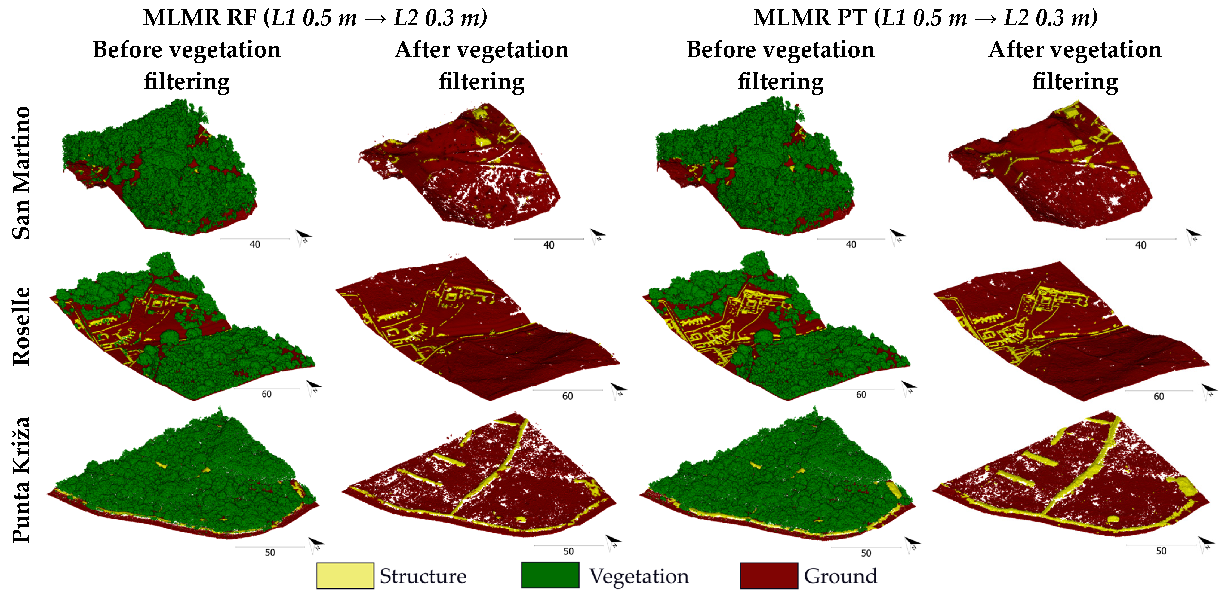
The comparison between RF and PT (Table 3 and Table 4 and Figure 3) shows an improvement in accuracy upon passing from the ML to the DL backbone. While at L1 (Table 3), the class scores for the non-vegetation (DFM) and vegetation classes are comparable, with RF slightly behind PT at both resolutions. At L2 (Table 4), PT significantly outperforms RF in structure detection (IoU scores of 51.77%, 51.83%, 56.32% vs. 33.48%, 36.53%, 46.03% respectively). Despite these results, RF achieves good overall performance at L1, particularly given its much shorter training time.
Table 3.
L1 metrics are computed on the test set, which comprises manually selected portions from all three datasets.
Table 4.
L2 metrics are computed on the test set, comprising manually selected portions from all three datasets, with the remaining post-L1 vegetation merged into the ground class in the GT to isolate L2 performance. * visuals in Figure 3.
Figure 3.
Results of both MLMR pipelines (L1 0.5 m → L2 0.3 m) on all three test sets. Scale bars in metres.
4.2. Comparison 2: MLMR Framework vs. End-to-End Approach
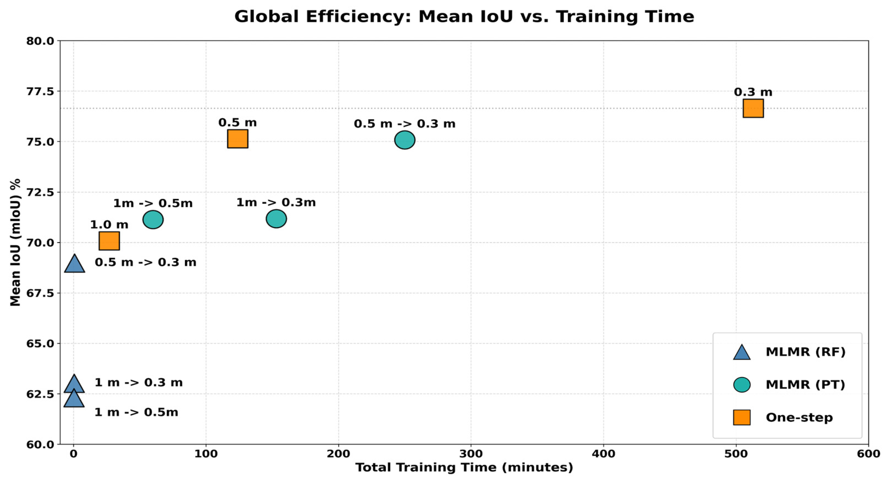
The comparison between the MLMR framework and the end-to-end approach with the PT backbone (Table 5) shows both approaches reaching similar average IoU scores, with the best MLMR configuration (L1 0.5 m → L2 0.3 m, 75.08% avg IoU) requiring 4 h 10 min compared with the 8 h 33 min needed for the best end-to-end approach (0.3 m).
Table 5.
MLMR and end-to-end approaches metrics were computed on the test set, comprising manually selected portions from all three datasets.
For both methods, the class structure yields the lowest scores. At the same time, the segmentation of ground and vegetation achieves high IoU scores, with the ground class IoU values ranging from 75.51% to 83.41% and the vegetation class IoU values ranging from 92.13% to 95.12%.
Processing at 1 m resolution significantly hampers results for both pipelines. The end-to-end approach at 1 m achieves the worst overall performance (70.08% average IoU, 42.59% structure IoU), while the MLMR pipelines using 1 m resolution at L1 reach intermediate structure class IoU scores (44.52–44.70%). Increasing resolution from 1 m to 0.5 m yields a substantial improvement in structure IoU for both approaches, as visible in the structure class IoU scores of the end-to-end approach configurations at 0.5 m and 0.3 m (51.92% and 51.42% respectively), and of the MLMR PT (L1 0.5 m → L2 0.3 m) configuration (50.64%). Surprisingly, the highest structure IoU is achieved by the end-to-end approach at 0.5 m resolution (51.92%, 2 h 4 min), outperforming both the 0.3 m end-to-end result (51.42%) and the best MLMR configuration (50.64%), making it the most cost-effective solution.
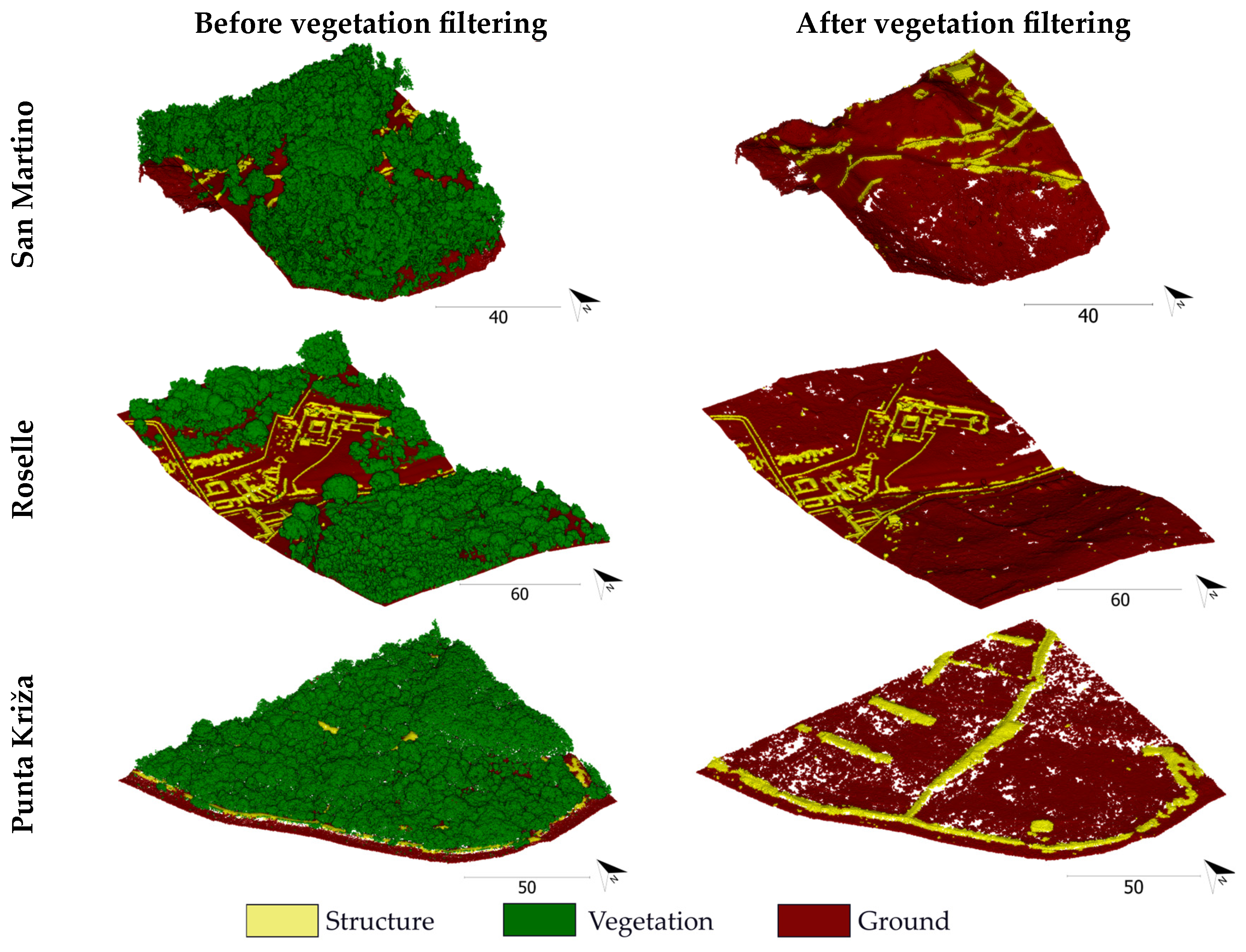
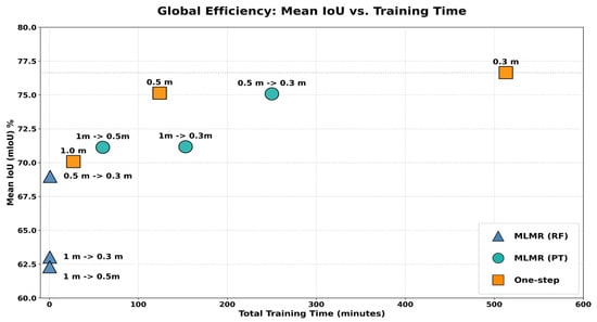
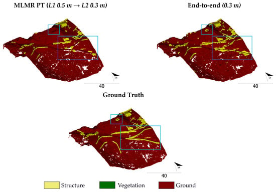
Figure 4 shows visual classification results across all three datasets for the end-to-end configuration at the highest resolution, whereas the full picture of the performance/cost combination for all configurations of both approaches is shown in Figure 5.
Figure 4.
Results of the end-to-end approach at 0.3 m resolution on all three test sets. Scale bars in metres.
Figure 5.
Efficiency of both MLMR (RF and PT) and end-to-end (PT) approaches, comparing average IoU scores with training time.
5. Discussions
Building on the results presented in Section 4, this discussion section analyses their implications for archaeological DFM workflows, with supporting visual examples.
5.1. Random Forest vs. Point Transformer
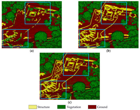
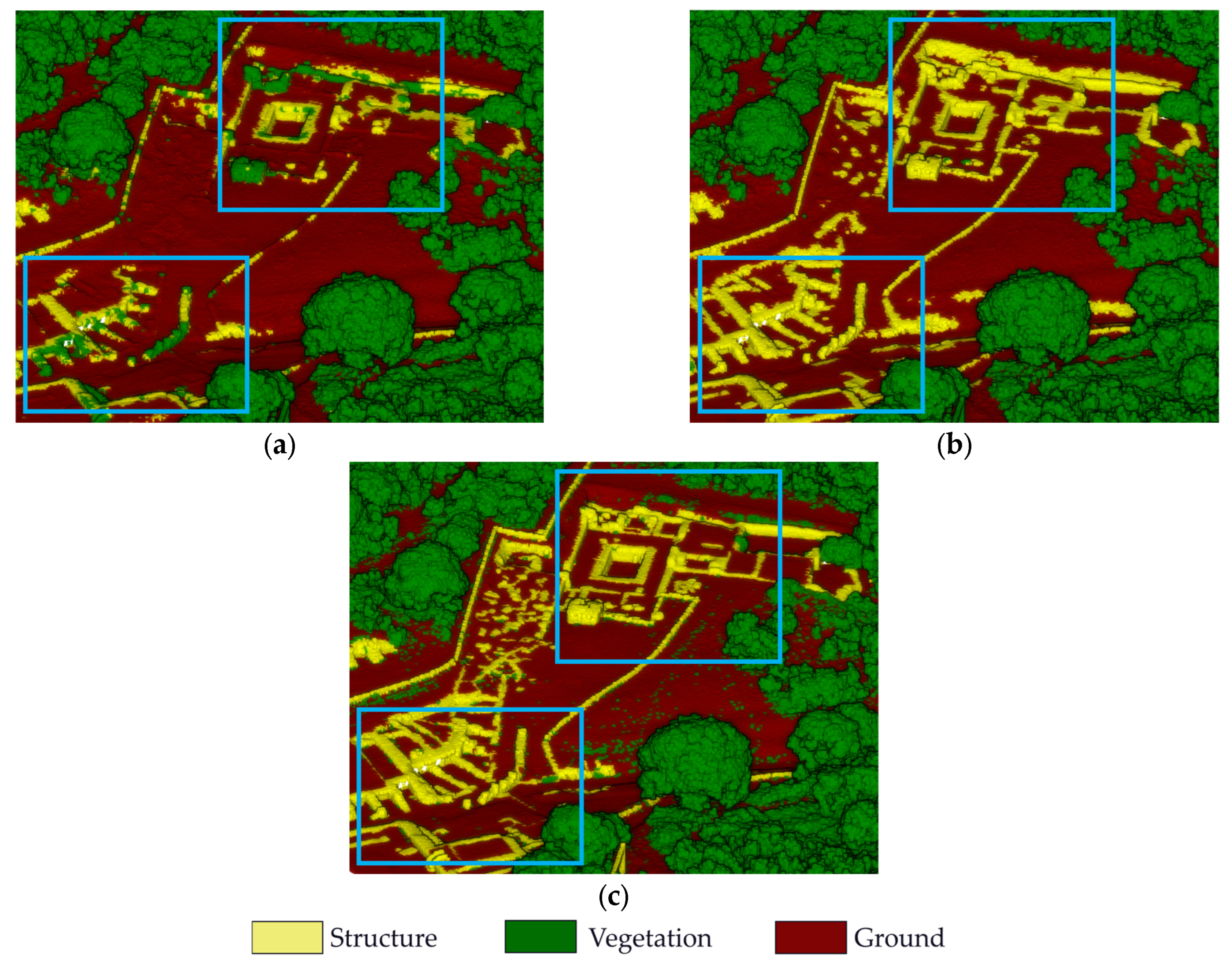
The accuracy gap between PT and RF highlights the limits of the standard ML configurations with handcrafted geometric features. RF-based configurations work well for segmenting classes with consistent geometric signatures, such as vegetation and ground, but struggle with the variable geometric patterns of archaeological structures. While more thorough feature selection could improve RF results, PT’s self-attention mechanism appears to better capture spatial relationships, resulting in improved performance on this challenging class. This is evident in Figure 6, where points belonging to the structure class in the GT (Figure 6c) are frequently misclassified as vegetation in the MLMR RF pipeline (Figure 6a), while they are, for the most part, correctly segmented in the MLMR PT pipeline (Figure 6b).
Figure 6.
Visual comparison between the RF MLMR (L1 0.5 m → L2 0.3 m) and the PT MLMR (the L1 0.5 m → L2 0.3 m) segmentation results for the structure class on the Roselle dataset: (a) MLMR RF prediction; (b) MLMR PT prediction; (c) GT. Blue boxes indicate the main classification errors and differences.
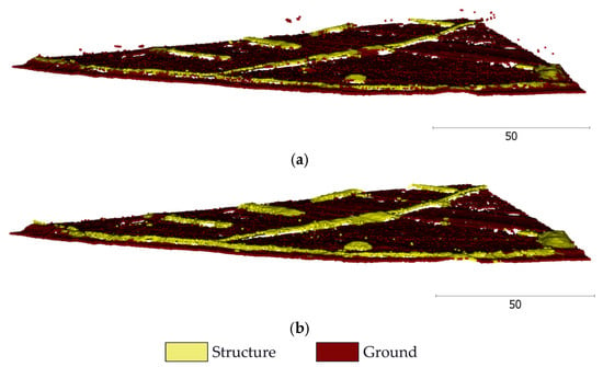
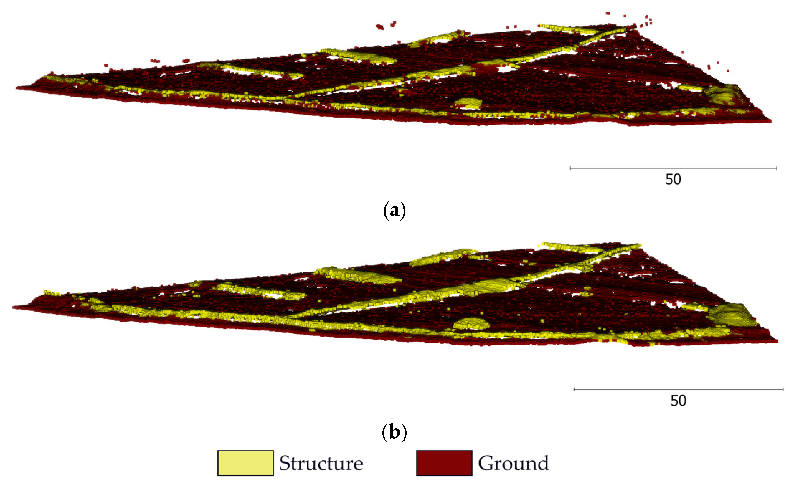
Another noteworthy limitation is that RF-based approaches exhibit higher surface noise after vegetation filtering (Figure 7a) compared to PT-based approaches (Figure 7b). This limitation hinders the possibility of extending MLMR with RF to large-scale applications, as extensive manual corrections or post-processing are required to produce a clean DFM.
Figure 7.
MLMR L1 0.5 m → L2 0.3 m results after vegetation filtering on the Punta Križa dataset: (a) RF prediction, (b) PT prediction. Scale bars in metres.
Despite these limitations, RF’s minimal training overhead (less than a minute compared to several hours for high-resolution PT configurations) and efficient ground and vegetation segmentation make RF a viable choice for exploratory studies where time and hardware constraints prevent the use of DL architecture.
5.2. MLMR vs. End-to-End Approach
Having established PT’s accuracy superiority, we next examine whether its hierarchical MLMR implementation offers advantages over an end-to-end processing pipeline.
The comparison between the MLMR framework and the end-to-end approach reveals distinct performance characteristics (Table 5). End-to-end segmentation achieves optimal results at the 0.5 m resolution, with higher resolutions increasing computational cost for minimal accuracy gain, even causing slight accuracy loss for the structure class. This suggests that, for the studied datasets, 0.5 m resolution provides an optimal balance between geometric detail and spatial consistency for structure detection, while 0.3 m processing reaches diminishing returns. Multiple factors may influence these outcomes. The heterogeneous point density across test sites (16 pts/m2 for Punta Križa vs. 500–750 pts/m2 for San Martino and Roselle) may contribute to this pattern. The Punta Križa dataset approaches its resolution limits at 0.3 m and, given that its optimal resolution for DFM interpolation has been reported at 0.5 m by Doneus et al. [74], the sparse point distribution at 0.3 m could hamper the architecture’s capability to understand the scene correctly, leading to lower performance than expected at the finer resolution.
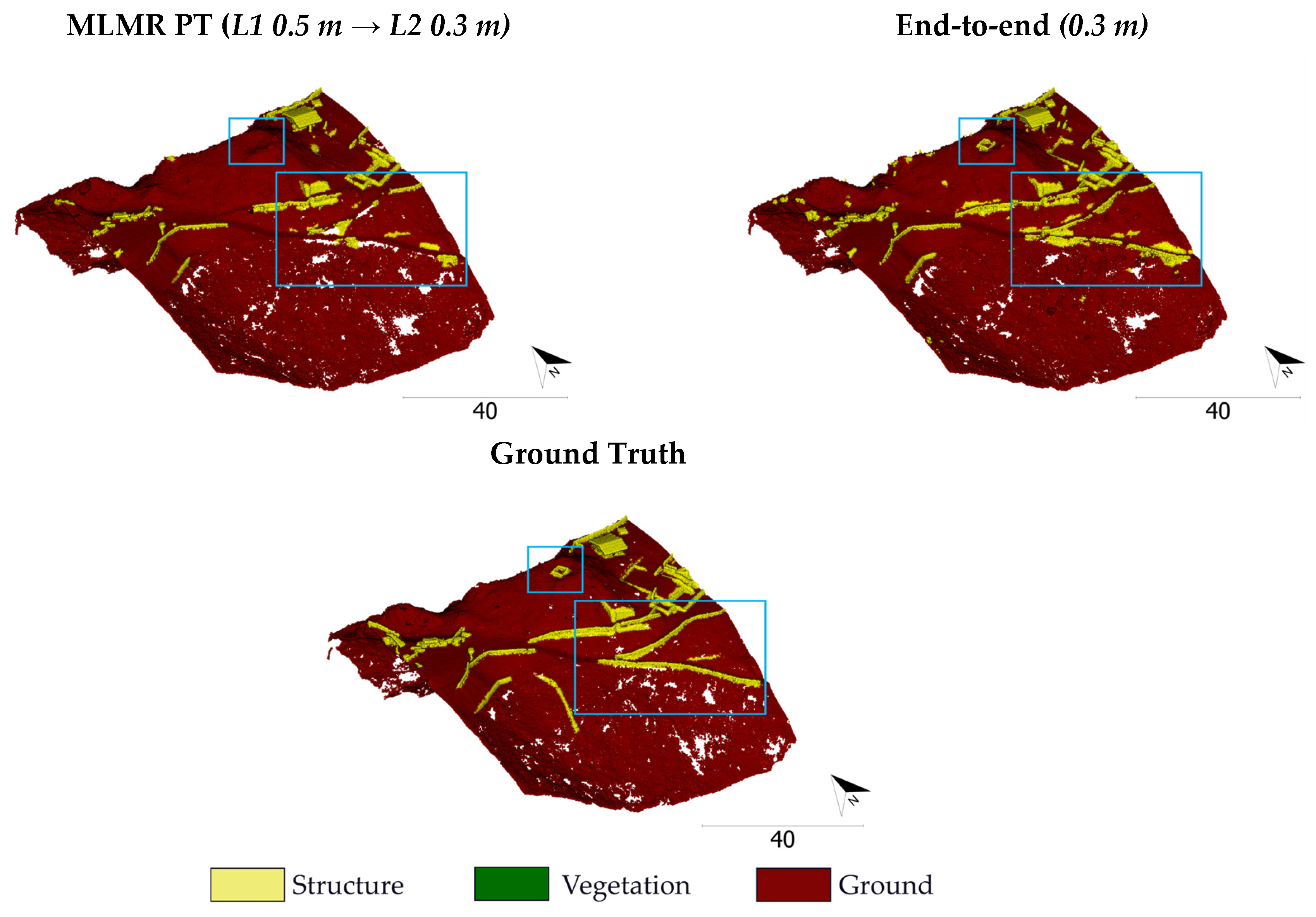
For the MLMR approach, while L1 achieves high vegetation segmentation accuracy, comparable to the end-to-end results, the use of a hard filtering procedure across pipeline levels results in some archaeological structures being misclassified as vegetation and filtered out. This is further demonstrated by the higher precision (66–70% compared to end-to-end’s 59–68%) but lower recall scores (56–64% for MLMR vs. 61–71% for end-to-end) on the structure class in comparison with the end-to-end approach, deriving from errors leaking from L1 results, despite the use of the training–test consistency strategy. This precision-recall trade-off is evident in Figure 8, where end-to-end predictions exhibit higher surface noise but better structure retention than MLMR.
Figure 8.
Comparison of DFM with structures prediction vs. ground truth. Blue boxes indicate the main classification errors and differences.
One advantage of the modular structure of the MLMR pipeline is that, by filtering vegetation at L1 (~74% of points), L2 processes drastically fewer points while focusing on the archaeologically critical distinction between structure/ground classes. While in this study, no improvement in structure detection is visible above the 0.5 m threshold, in cases where very subtle archaeological features require higher resolution, the modular nature of the approach could reduce time and hardware constraints while achieving results comparable to processing the whole point cloud at a higher resolution.
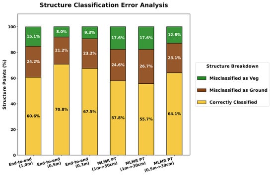
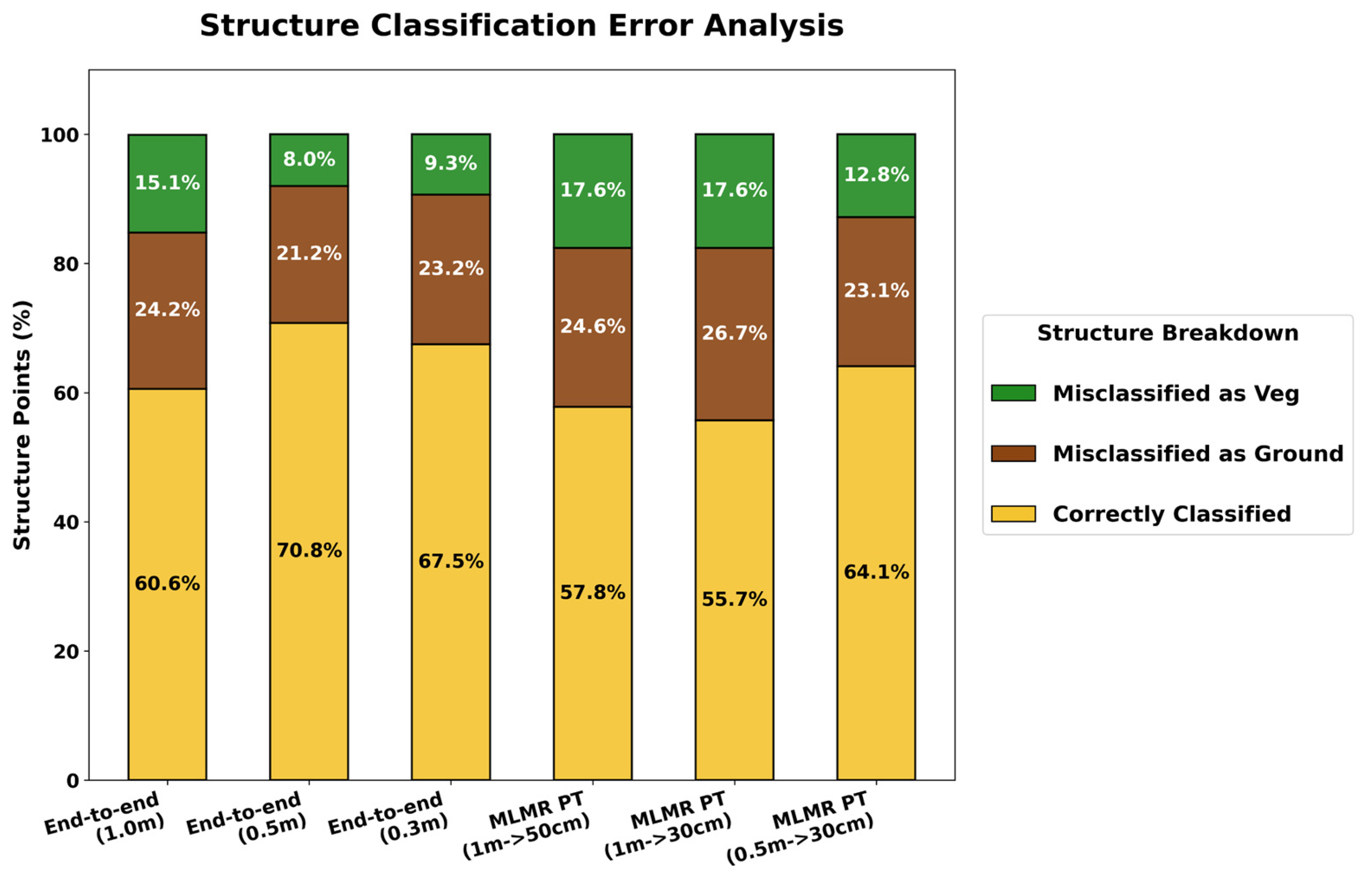
Both approaches yield similar results for the structure class, with most misclassifications occurring with the ground class, as shown in Figure 9. This suggests that the challenging nature of this task is not related to the use of either the MLMR or the end-to-end approach to process the data, but rather to the similarity in geometry between the two classes.
Figure 9.
Structure points misclassification was calculated from the confusion matrix of the six DL configurations’ predictions on the test set.
Although these results show trade-offs between the two methodologies, it is worth mentioning that some aspects of the MLMR approach have not been fully explored within the current experimental setup.
To ensure a fair comparison, this study uses the same architecture for both approaches, but this is not necessarily the best configuration for the MLMR approach; adopting other architectures or a combination of architectures at each pipeline level could better exploit the methodology’s modular structure. Moreover, uniform hyperparameters are employed across all configurations. However, MLMR’s modular architecture enables task-specific optimisation opportunities not explored here, such as specialised loss functions (e.g., Focal Loss for the structure class), class weights, or level-specific feature selection, which could potentially narrow the performance gap while keeping the computational advantage, given the fundamental data reduction at L1.
6. Conclusions
Building upon the results of our prior work, in this study, we propose an MLMR approach for the generation of archaeological DFMs with already mapped archaeological structures, alongside a novel train–test consistency strategy to train the second level of the pipeline. To assess the methodology’s performance, two comparisons are performed across diverse datasets with varying acquisition conditions and archaeological features: first, the hierarchical MLMR approach is tested using different backbones (RF and PT) and evaluated through quantitative and qualitative analyses. Second, the MLMR approach is compared against an end-to-end approach, where all classes are predicted in a single passage (both using the same PT backbone) to evaluate the trade-offs between the two methodologies.
The first comparison reveals substantial improvements when using PT as the MLMR backbone over RF, boosting semantic segmentation accuracy at both pipeline levels, especially for the structure class at L2. This improvement comes at a computational cost, with RF notably more efficient in terms of training time.
The comparison between the hierarchical MLMR and end-to-end approaches shows that both pipelines achieve similar results at similar resolutions, albeit with a precision-recall trade-off in structure mapping. MLMR achieves a higher precision but lower recall, while the end-to-end approach trades precision for a higher recall. While overall results are very close, the most cost-effective approach for this dataset is the end-to-end approach at 0.5 m, achieving the highest structure class IoU with half the training time of the highest-scoring MLMR approach and less than one-fourth the time of the end-to-end approach at 0.3 m resolution. These results show that increasing resolution can result in substantial computational expense with minimal accuracy gains.
While the end-to-end approach at 0.5 m offers the best balance of accuracy and efficiency on these specific datasets, MLMR can be advantageous at finer resolutions (0.3 m) when greater detail for archaeological analysis is needed, or when interpretability, progressive validation, and specific segmentation strategies for each level are considered:
- Interpretability allows identification of the stage at which errors occur, enabling targeted improvements.
- Progressive validation allows validating L1 outputs before committing to L2 processing.
- Specific segmentation strategies allow for maximising each level of the pipeline.
Future research should address limitations and opportunities identified in this study:
- Comparative evaluation across multiple DL architectures (KPConv, PointNet++, Superpoint Transformer, etc.) is necessary to assess their performance on archaeological LiDAR data and identify which architectures are most suitable for each pipeline level.
- Task-specific optimisation of MLMR levels with specialised loss functions, sampling strategies, batch sizes, and adaptive class weights could maximise outcomes at each level.
- The exploration of modular generalisability, where an L1 model trained on diverse vegetation types could be applied to new datasets without retraining, substantially reduces data requirements while leaving archaeological-specific segmentation to L2.
- Evaluation of segmentation outcomes through analysis of generated DFM rasters, assessing archaeological feature detection, mapping accuracy, and microrelief visibility.
Author Contributions
Conceptualisation, G.M. and F.R.; methodology, G.M.; software, G.M.; validation, G.M.; formal analysis, G.M.; investigation, G.M.; resources, F.R.; data curation, G.M.; writing—original draft preparation, G.M.; writing—review and editing, G.M. and F.R.; visualisation, G.M.; supervision, F.R.; project administration, F.R.; funding acquisition, F.R. All authors have read and agreed to the published version of the manuscript.
Funding
This research received no external funding.
Data Availability Statement
Datasets employed in the paper are available on demand for research purposes.
Acknowledgments
Authors are thankful to Prof. Michael Doneus—Department of Prehistoric and Historical Archaeology of the University of Vienna (Austria) and to Prof. Stefano Campana—Department of History and Cultural Heritage of the University of Siena (Italy) for sharing the Punta Križa and Roselle datasets for this research.
Conflicts of Interest
The authors declare no conflicts of interest.
Abbreviations
The following abbreviations are used in this manuscript:
| ALS | Airborne Laser Scanning |
| DL | Deep Learning |
| DFM | Digital Feature Model |
| DTM | Digital Terrain Model |
| GPU | Graphics Processing Unit |
| GT | Ground Truth |
| IoU | Intersection over Union |
| L1 | Level 1 |
| L2 | Level 2 |
| UAV | Unmanned Aerial Vehicle UAV |
| LiDAR | Light Detection And Ranging |
| ML | Machine Learning |
| MLMR | Multi-Level Multi-Resolution |
| RF | Random Forest |
| PT | Point Transformer |
| VT | Visualisation Technique |
Notes
| 1 | LAStools, rapidlasso GmbH. http://rapidlasso.com/LAStools. |
| 2 | TerraScan, Terrasolid Ltd., Helsinki, Finland. https://terrasolid.com. |
| 3 | PDAL: Point Data Abstraction Library. https://pdal.io. |
| 4 | CloudCompare. https://www.cloudcompare.org. |
| 5 | RAPIDS cuML: https://github.com/rapidsai/cuml. |
| 6 | scikit-learn: https://scikit-learn.org. |
References
- Opitz, R.S.; Cowley, D.C. Interpreting archaeological topography: Lasers, 3D data, observation, visualisation and applications. In Interpreting Archaeological Topography: 3D Data, Visualisation and Observation; Oxbow Books: Oxford, UK, 2013; pp. 1–12. [Google Scholar]
- Campana, S.R. Mapping the Archaeological Continuum: Filling ‘Empty’ Mediterranean Landscapes; Springer: New York, NY, USA, 2018. [Google Scholar]
- Johnson, K.M.; Ouimet, W.B. An observational and theoretical framework for interpreting the landscape palimpsest through airborne LiDAR. Appl. Geogr. 2018, 91, 32–44. [Google Scholar] [CrossRef] [Scilit]
- Vinci, G.; Vanzani, F.; Fontana, A.; Campana, S. LiDAR applications in archaeology: A systematic review. Archaeol. Prospect. 2025, 32, 81–101. [Google Scholar] [CrossRef] [Scilit]
- Pingel, T.J.; Clarke, K.; Ford, A. Bonemapping: A LiDAR processing and visualization technique in support of archaeology under the canopy. Cartogr. Geogr. Inf. Sci. 2015, 42, 18–26. [Google Scholar] [CrossRef] [Scilit]
- Štular, B.; Lozić, E.; Eichert, S. Airborne LiDAR-derived digital elevation model for archaeology. Remote Sens. 2021, 13, 1855. [Google Scholar] [CrossRef] [Scilit]
- Doneus, M.; Banaszek, Ł.; Verhoeven, G.J. The impact of vegetation on the visibility of archaeological features in airborne laser scanning datasets from different acquisition dates. Remote Sens. 2022, 14, 858. [Google Scholar] [CrossRef] [Scilit]
- Cirigliano, G.P.; Mazzacca, G.; Remondino, F.; Liverani, P.; Cantoro, G.; Maschner, H.; Campana, S. Drone-Based High-Resolution LiDAR for Undercanopy Archaeology in Mediterranean Environment: Rusellae Case Study (Italy). Archaeol. Prospect. 2025, 32, 644–655. [Google Scholar] [CrossRef] [Scilit]
- Hyyppä, H.; Yu, X.; Hyyppä, J.; Kaartinen, H.; Kaasalainen, S.; Honkavaara, E.; Rönnholm, P. Factors affecting the quality of DTM generation in forested areas. Int. Arch. Photogramm. Remote Sens. Spat. Inf. Sci. 2005, 36, 85–90. [Google Scholar]
- Doneus, M.; Mandlburger, G.; Doneus, N. Archaeological ground point filtering of airborne laser scan derived point-clouds in a difficult mediterranean environment. J. Comput. Appl. Archaeol. 2020, 3, 92–108. [Google Scholar] [CrossRef] [Scilit]
- Teruggi, S.; Grilli, E.; Russo, M.; Fassi, F.; Remondino, F. A hierarchical machine learning approach for multi-level and multi-resolution 3D point cloud classification. Remote Sens. 2020, 12, 2598. [Google Scholar] [CrossRef] [Scilit]
- Zhang, K.; Teruggi, S.; Fassi, F. Machine learning methods for Unesco Chinese heritage: Complexity and comparisons. Int. Arch. Photogramm. Remote Sens. Spat. Inf. Sci. 2022, 46, 543–550. [Google Scholar] [CrossRef] [Scilit]
- Chehata, N.; Guo, L.; Mallet, C. Airborne lidar feature selection for urban classification using random forests. In Laserscanning; ISPRS: Paris, France, 2009. [Google Scholar]
- Zhao, H.; Jiang, L.; Jia, J.; Torr, P.H.; Koltun, V. Point transformer. In Proceedings of the IEEE/CVF International Conference on Computer Vision, Montreal, QC, Canada, 10–17 October 2021; IEEE Computer Society: Washington, DC, USA, 2021; pp. 16259–16268. [Google Scholar]
- Mazzacca, G.; Grilli, E.; Cirigliano, G.P.; Remondino, F.; Campana, S. Seeing among foliage with lidar and machine learning: Towards a transferable archaeological pipeline. Int. Arch. Photogramm. Remote Sens. Spat. Inf. Sci. 2022, 46, 365–372. [Google Scholar] [CrossRef] [Scilit]
- Holden, N. Digital airborne remote sensing: The principles of LIDAR and CASI. AARGNews 2001, 22, 23. [Google Scholar]
- Sittler, B. Revealing historical landscapes by using airborne laser scanning. Int. Arch. Photogramm. Remote Sens. Spat. Inf. Sci. 2004, 36, 258–261. [Google Scholar]
- Devereux, B.J.; Amable, G.S.; Crow, P.; Cliff, A.D. The potential of airborne lidar for detection of archaeological features under woodland canopies. Antiquity 2005, 79, 648–660. [Google Scholar] [CrossRef] [Scilit]
- Bofinger, J.; Kurz, S.; Schmidt, S. Ancient Maps-modern data sets: Different investigative techniques in the landscape of the Early Iron Age princely hill fort Heuneburg, Baden-Wurttemberg. BAR Int. Ser. 2006, 1568, 87. [Google Scholar]
- Evans, D.H.; Fletcher, R.J.; Pottier, C.; Chevance, J.B.; Soutif, D.; Tan, B.S.; Im, S.; Ea, D.; Tin, T.; Kim, S.; et al. Uncovering archaeological landscapes at Angkor using lidar. Proc. Natl. Acad. Sci. USA 2013, 110, 12595–12600. [Google Scholar] [CrossRef] [Scilit]
- Canuto, M.A.; Estrada-Belli, F.; Garrison, T.G.; Houston, S.D.; Acuña, M.J.; Kováč, M.; Marken, D.; Nondédéo, P.; Auld-Thomas, L.; Castanet, C.; et al. Ancient lowland Maya complexity as revealed by airborne laser scanning of northern Guatemala. Science 2018, 361, eaau0137. [Google Scholar] [CrossRef] [Scilit]
- Estrada-Belli, F.; Gilabert-Sansalvador, L.; Canuto, M.A.; Šprajc, I.; Fernandez-Diaz, J.C. Architecture, wealth and status in Classic Maya urbanism revealed by airborne lidar mapping. J. Archaeol. Sci. 2023, 157, 105835. [Google Scholar] [CrossRef] [Scilit]
- Sánchez Polo, A.; Álvarez Litben, R. Un paisaje monumental prehispánico en la Alta Amazonía ecuatoriana: Primeros resultados de la aplicación de Lidar en el valle del Upano. Strata. Rev. Ecuat. Arqueol. Paleontol. 2023, 1, e3. [Google Scholar]
- Chase, A.F.; Chase, D.Z.; Weishampel, J.F.; Drake, J.B.; Shrestha, R.L.; Slatton, K.C.; Awe, J.J.; Carter, W.E. Airborne LiDAR, archaeology, and the ancient Maya landscape at Caracol, Belize. J. Archaeol. Sci. 2011, 38, 387–398. [Google Scholar] [CrossRef] [Scilit]
- Chase, A.F.; Chase, D.Z.; Awe, J.J.; Weishampel, J.F.; Iannone, G.; Moyes, H.; Yaeger, J.; Brown, M.K.; Shrestha, R.L.; Carter, W.E.; et al. Ancient Maya regional settlement and inter-site analysis: The 2013 west-central Belize LiDAR survey. Remote Sens. 2014, 6, 8671–8695. [Google Scholar] [CrossRef] [Scilit]
- Garrison, T.G.; Houston, S.; Firpi, O.A. Recentering the rural: Lidar and articulated landscapes among the Maya. J. Anthropol. Archaeol. 2019, 53, 133–146. [Google Scholar] [CrossRef] [Scilit]
- Auld-Thomas, L.; Canuto, M.A.; Morlet, A.V.; Estrada-Belli, F.; Chatelain, D.; Matadamas, D.; Pigott, M.; Díaz, J.C.F. Running out of empty space: Environmental lidar and the crowded ancient landscape of Campeche, Mexico. Antiquity 2024, 98, 1340–1358. [Google Scholar] [CrossRef] [Scilit]
- Estrada-Belli, F.; Canuto, M.A.; Šprajc, I.; Fernandez-Diaz, J.C. New regional-scale Classic Maya population density estimates and settlement distribution models through airborne lidar scanning. J. Archaeol. Sci. 2025, 66, 105288. [Google Scholar] [CrossRef] [Scilit]
- Evans, D. Airborne laser scanning as a method for exploring long-term socio-ecological dynamics in Cambodia. J. Archaeol. Sci. 2016, 74, 164–175. [Google Scholar] [CrossRef] [Scilit]
- Chevance, J.B.; Evans, D.; Hofer, N.; Sakhoeun, S.; Chhean, R. Mahendraparvata: An early Angkor-period capital defined through airborne laser scanning at Phnom Kulen. Antiquity 2019, 93, 1303–1321. [Google Scholar] [CrossRef] [Scilit]
- Klassen, S.; Carter, A.K.; Evans, D.H.; Ortman, S.; Stark, M.T.; Loyless, A.A.; Polkinghorne, M.; Heng, P.; Hill, M.; Wijker, P.; et al. Diachronic modeling of the population within the medieval Greater Angkor Region settlement complex. Sci. Adv. 2021, 7, eabf8441. [Google Scholar] [CrossRef] [Scilit]
- Forlin, P. Airborne LiDAR data analysis within the Alpine landscapes of Trentino: A methodological approach. Post-Class. Archaeol. 2012, 2, 247–268. [Google Scholar]
- Bernardini, F.; Vinci, G.; Horvat, J.; De Min, A.; Forte, E.; Furlani, S.; Lenaz, D.; Pipan, M.; Zhao, W.; Sgambati, A.; et al. Early Roman military fortifications and the origin of Trieste, Italy. Proc. Natl. Acad. Sci. USA 2015, 112, E1520–E1529. [Google Scholar] [CrossRef] [Scilit]
- Vinci, G.; Bernardini, F. Reconstructing the protohistoric landscape of Trieste Karst (north-eastern Italy) through airborne LiDAR remote sensing. J. Archaeol. Sci. 2017, 12, 591–600. [Google Scholar] [CrossRef] [Scilit]
- Sánchez, J.G. Archaeological LiDAR in Italy: Enhancing research with publicly accessible data. Antiquity 2018, 92, e4. [Google Scholar] [CrossRef] [Scilit]
- Bewley, R.H.; Crutchley, S.P.; Shell, C.A. New light on an ancient landscape: Lidar survey in the Stonehenge World Heritage Site. Antiquity 2005, 79, 636–647. [Google Scholar] [CrossRef] [Scilit]
- Crutchley, S.; Crow, P. Using Airborne LiDAR in Archaeological Survey: The Light Fantastic; Historic England: London, UK, 2018.
- Cowley, D.; Banaszek, Ł.; Geddes, G.; Gannon, A.; Middleton, M.; Millican, K. Making LiGHT work of large area survey? Developing approaches to rapid archaeological mapping and the creation of systematic national-scaled heritage data. J. Comput. Appl. Archaeol. 2020, 3, 109–121. [Google Scholar] [CrossRef] [Scilit]
- Cerrillo-Cuenca, E.; Bueno-Ramírez, P. Counting with the invisible record? The role of LiDAR in the interpretation of megalithic landscapes in south-western Iberia (Extremadura, Alentejo and Beira Baixa). Archaeol. Prospect. 2019, 26, 251–264. [Google Scholar] [CrossRef] [Scilit]
- Menéndez Blanco, A.; García Sánchez, J.; Costa-García, J.M.; Fonte, J.; González-Álvarez, D.; Vicente García, V. Following the Roman Army between the Southern Foothills of the Cantabrian Mountains and the Northern Plains of Castile and León (North of Spain): Archaeological applications of remote sensing and geospatial tools. Geosciences 2020, 10, 485. [Google Scholar] [CrossRef] [Scilit]
- Rodríguez González, E.; Paniego Díaz, P.; Celestino Pérez, S. Lost Landscape: A Combination of LiDAR and APSFR Data to Locate and Contextualize Archaeological Sites in River Environments. Remote Sens. 2021, 13, 3506. [Google Scholar] [CrossRef] [Scilit]
- Evans, D.; Fletcher, R. The landscape of Angkor Wat redefined. Antiquity 2015, 89, 1402–1419. [Google Scholar] [CrossRef] [Scilit]
- Fontana, G. Italy’s hidden hillforts: A large-scale Lidar-based mapping of Samnium. J. Field Archaeol. 2022, 47, 245–261. [Google Scholar] [CrossRef] [Scilit]
- Sánchez, J.G.; Donnellan, L.; Fonte, J.; Stümpel, A.E.; Bintliff, J. Drone and airborne lidar in Greece: A Mediterranean perspective on processing techniques and cultural landscapes. J. Greek Archaeol. 2025, 10, 197–214. [Google Scholar] [CrossRef] [Scilit]
- Doneus, M.; Briese, C.; Fera, M.; Janner, M. Archaeological prospection of forested areas using full-waveform airborne laser scanning. J. Archaeol. Sci. 2008, 35, 882–893. [Google Scholar] [CrossRef] [Scilit]
- Crow, P.; Benham, S.; Devereux, B.J.; Amable, G.S. Woodland vegetation and its implications for archaeological survey using LiDAR. Forestry 2007, 80, 241–252. [Google Scholar] [CrossRef] [Scilit]
- Inomata, T.; Pinzón, F.; Ranchos, J.L.; Haraguchi, T.; Nasu, H.; Fernandez-Diaz, J.C.; Aoyama, K.; Yonenobu, H. Archaeological application of airborne LiDAR with object-based vegetation classification and visualization techniques at the lowland Maya site of Ceibal, Guatemala. Remote Sens. 2017, 9, 563. [Google Scholar] [CrossRef] [Scilit]
- Banaszek, Ł. It takes all kinds of trees to make a forest. Using historic maps and forestry data to inform airborne laser scanning based archaeological prospection in woodland. Archaeol. Prospect. 2020, 27, 377–392. [Google Scholar] [CrossRef] [Scilit]
- Doneus, M. Openness as visualization technique for interpretative mapping of airborne lidar derived digital terrain models. Remote Sens. 2013, 5, 6427–6442. [Google Scholar] [CrossRef] [Scilit]
- Kokalj, Ž.; Hesse, R. Airborne Laser Scanning Raster Data Visualization: A Guide to Good Practice; Založba ZRC: Ljubljana, Slovenia, 2017; Volume 14. [Google Scholar]
- Kokalj, Ž.; Somrak, M. Why not a single image? Combining visualizations to facilitate fieldwork and on-screen mapping. Remote Sens. 2019, 11, 747. [Google Scholar] [CrossRef] [Scilit]
- Bennett, R.; Cowley, D.; De Laet, V. The data explosion: Tackling the taboo of automatic feature recognition in airborne survey data. Antiquity 2014, 88, 896–905. [Google Scholar] [CrossRef] [Scilit]
- Schneider, A.; Takla, M.; Nicolay, A.; Raab, A.; Raab, T. A template-matching approach combining morphometric variables for automated mapping of charcoal kiln sites. Archaeol. Prospect. 2015, 22, 45–62. [Google Scholar] [CrossRef] [Scilit]
- Meyer, M.F.; Pfeffer, I.; Jürgens, C. Automated detection of field monuments in digital terrain models of Westphalia using OBIA. Geosciences 2019, 9, 109. [Google Scholar] [CrossRef] [Scilit]
- Guyot, A.; Hubert-Moy, L.; Lorho, T. Detecting Neolithic burial mounds from LiDAR-derived elevation data using a multi-scale approach and machine learning techniques. Remote Sens. 2018, 10, 225. [Google Scholar] [CrossRef] [Scilit]
- Niculiță, M. Geomorphometric methods for burial mound recognition and extraction from high-resolution LiDAR DEMs. Sensors 2020, 20, 1192. [Google Scholar] [CrossRef] [Scilit]
- Trier, Ø.D.; Reksten, J.H.; Løseth, K. Automated mapping of cultural heritage in Norway from airborne lidar data using faster R-CNN. Int. J. Appl. Earth Obs. Geoinf. 2021, 95, 102241. [Google Scholar] [CrossRef] [Scilit]
- Verschoof-van der Vaart, W.B.; Lambers, K. Applying automated object detection in archaeological practice: A case study from the southern Netherlands. Archaeol. Prospect. 2022, 29, 15–31. [Google Scholar] [CrossRef] [Scilit]
- Berganzo-Besga, I.; Orengo, H.A.; Lumbreras, F.; Carrero-Pazos, M.; Fonte, J.; Vilas-Estévez, B. Hybrid MSRM-based deep learning and multitemporal sentinel 2-based machine learning algorithm detects near 10k archaeological tumuli in North-Western Iberia. Remote Sens. 2021, 13, 4181. [Google Scholar] [CrossRef] [Scilit]
- Štular, B.; Lozić, E.; Eichert, S. Interpolation of airborne LiDAR data for archaeology. J. Archaeol. Sci. 2023, 48, 103840. [Google Scholar] [CrossRef] [Scilit]
- De Boer, A.G.; Laan, W.N.; Waldus, W.; Van Zijverden, W.K. LIDAR-based surface height measurements: Applications in archaeology. In Beyond Illustration: 2D and 3D Digital Technologies as Tools for Discovery in Archaeology; Frischer, B., Dakouri-Hild, A., Eds.; BAR Publishing: Oxford, UK, 2008; pp. 76–84. [Google Scholar]
- Fernandez-Diaz, J.C.; Carter, W.E.; Shrestha, R.L.; Glennie, C.L. Now you see it… now you don’t: Understanding airborne mapping LiDAR collection and data product generation for archaeological research in Mesoamerica. Remote Sens. 2014, 6, 9951–10001. [Google Scholar] [CrossRef] [Scilit]
- Lozić, E.; Štular, B. Documentation of archaeology-specific workflow for airborne LiDAR data processing. Geosciences 2021, 11, 26. [Google Scholar] [CrossRef] [Scilit]
- Axelsson, P. DEM generation from laser scanner data using adaptive TIN models. Int. Arch. Photogramm. Remote Sens. 2000, 33, 110–117. [Google Scholar]
- Zhang, K.; Chen, S.C.; Whitman, D.; Shyu, M.L.; Yan, J.; Zhang, C. A progressive morphological filter for removing nonground measurements from airborne LIDAR data. IEEE Trans. Geosci. Remote Sens. 2003, 41, 872–882. [Google Scholar] [CrossRef] [Scilit]
- Zhang, W.; Qi, J.; Wan, P.; Wang, H.; Xie, D.; Wang, X.; Yan, G. An easy-to-use airborne LiDAR data filtering method based on cloth simulation. Remote Sens. 2016, 8, 501. [Google Scholar] [CrossRef] [Scilit]
- Sithole, G.; Vosselman, G. Experimental comparison of filter algorithms for bare-Earth extraction from airborne laser scanning point clouds. ISPRS J. Photogramm. Remote Sens. 2004, 59, 85–101. [Google Scholar]
- Meng, X.; Currit, N.; Zhao, K. Ground filtering algorithms for airborne LiDAR data: A review of critical issues. Remote Sens. 2010, 2, 833–860. [Google Scholar] [CrossRef] [Scilit]
- Štular, B.; Lozić, E. Comparison of filters for archaeology-specific ground extraction from airborne LiDAR point clouds. Remote Sens. 2020, 12, 3025. [Google Scholar] [CrossRef] [Scilit]
- Doneus, M.; Höfle, B.; Kempf, D.; Daskalakis, G.; Shinoto, M. Human-in-the-loop development of spatially adaptive ground point filtering pipelines—An archaeological case study. Archaeol. Prospect. 2022, 29, 503–524. [Google Scholar] [CrossRef] [Scilit]
- Richards-Rissetto, H.; Newton, D.; Al Zadjali, A. A 3D point cloud deep learning approach using lidar to identify ancient maya archaeological sites. In Proceedings of the 2021 28th CIPA Symposium “Great Learning & Digital Emotion”, Beijing, China, 28 August–1 September 2021. [Google Scholar]
- Cai, Z.; Vasconcelos, N. Cascade R-CNN: High quality object detection and instance segmentation. IEEE Trans. Pattern Anal. Mach. Intell. 2019, 43, 1483–1498. [Google Scholar] [CrossRef] [Scilit]
- Doneus, M.; Doneus, N.; Briese, C.; Pregesbauer, M.; Mandlburger, G.; Verhoeven, G. Airborne laser bathymetry–detecting and recording submerged archaeological sites from the air. J. Archaeol. Sci. 2013, 40, 2136–2151. [Google Scholar] [CrossRef] [Scilit]
- Doneus, M.; Doneus, N.; Cowley, D. Confronting complexity: Interpretation of a dry stone walled landscape on the island of Cres, Croatia. Land 2022, 11, 1672. [Google Scholar] [CrossRef] [Scilit]
- Bellosi, G.; Granata, A.; Pisu, N.; Christie, N.J.; Baker, P. The late antique and early medieval habitat and church on the Monte S. Martino, Riva del Garda district, north Italy. Mediev. Settl. Res. 2013, 28, 9–17. [Google Scholar]
- Campana, S. Emptyscapes: Filling an ‘empty’Mediterranean landscape at Rusellae, Italy. Antiquity 2017, 91, 1223–1240. [Google Scholar] [CrossRef] [Scilit]
- Pierdicca, R.; Paolanti, M.; Matrone, F.; Martini, M.; Morbidoni, C.; Malinverni, E.S.; Frontoni, E.; Lingua, A.M. Point cloud semantic segmentation using a deep learning framework for cultural heritage. Remote Sens. 2020, 12, 1005. [Google Scholar] [CrossRef] [Scilit]
- Matrone, F.; Grilli, E.; Martini, M.; Paolanti, M.; Pierdicca, R.; Remondino, F. Comparing machine and deep learning methods for large 3D heritage semantic segmentation. ISPRS Int. J. Geo-Inf. 2020, 9, 535. [Google Scholar] [CrossRef] [Scilit]
- Grilli, E.; Özdemir, E.; Remondino, F. Application of machine and deep learning strategies for the classification of heritage point clouds. Int. Arch. Photogramm. Remote Sens. Spat. Inf. Sci. 2019, 42, 447–454. [Google Scholar] [CrossRef] [Scilit]
- Croce, V.; Caroti, G.; De Luca, L.; Jacquot, K.; Piemonte, A.; Véron, P. From the semantic point cloud to heritage-building information modeling: A semiautomatic approach exploiting machine learning. Remote Sens. 2021, 13, 461. [Google Scholar] [CrossRef] [Scilit]
- Grilli, E.; Remondino, F. Machine learning generalisation across different 3D architectural heritage. ISPRS Int. J. Geo-Inf. 2020, 9, 379. [Google Scholar] [CrossRef] [Scilit]
- Bassier, M.; Mazzacca, G.; Battisti, R.; Malek, S.; Remondino, F. Combining image and point cloud segmentation to improve heritage understanding. Int. Arch. Photogramm. Remote Sens. Spat. Inf. Sci. 2024, 48, 49–56. [Google Scholar] [CrossRef] [Scilit]
- Sánchez-Aparicio, L.J.; Santamaría-Maestro, R.; Sanz-Honrado, P.; Villanueva-Llauradó, P.; Aira-Zunzunegui, J.R.; González-Aguilera, D. A holistic solution for supporting the diagnosis of historic constructions from 3D point clouds. Remote Sens. 2025, 17, 2018. [Google Scholar] [CrossRef] [Scilit]
- Betsas, T.; Tsarpalis, H.; Georgopoulos, A. Assessing Generalization Capability of 3D Semantic Segmentation Algorithms using 3D Point Clouds of Cultural Heritage. Int. Arch. Photogramm. Remote Sens. Spat. Inf. Sci. 2025, 48, 111–118. [Google Scholar] [CrossRef] [Scilit]
- Betsas, T.; Murtiyoso, A.; Grussenmeyer, P.; Georgopoulos, A. Exploring Point Transformers on 3D Semantic Segmentation of Javanese Architectures. Int. Arch. Photogramm. Remote Sens. Spat. Inf. Sci. 2026, 48, 57–64. [Google Scholar] [CrossRef] [Scilit]
- Weinmann, M.; Jutzi, B.; Hinz, S.; Mallet, C. Semantic point cloud interpretation based on optimal neighborhoods, relevant features and efficient classifiers. ISPRS J. Photogramm. Remote Sens. 2015, 105, 286–304. [Google Scholar] [CrossRef] [Scilit]
- Loshchilov, I.; Hutter, F. Decoupled weight decay regularization. arXiv 2017, arXiv:1711.05101. [Google Scholar]
- Berman, M.; Triki, A.R.; Blaschko, M.B. The lovász-softmax loss: A tractable surrogate for the optimization of the intersection-over-union measure in neural networks. In Proceedings of the IEEE Conference on Computer Vision and Pattern Recognition, Salt Lake City, UT, USA, 18–23 June 2018; IEEE: Piscataway, NJ, USA, 2018; pp. 4413–4421. [Google Scholar]

Disclaimer/Publisher’s Note: The statements, opinions and data contained in all publications are solely those of the individual author(s) and contributor(s) and not of MDPI and/or the editor(s). MDPI and/or the editor(s) disclaim responsibility for any injury to people or property resulting from any ideas, methods, instructions or products referred to in the content. |
© 2026 by the authors. Licensee MDPI, Basel, Switzerland. This article is an open access article distributed under the terms and conditions of the Creative Commons Attribution (CC BY) license.