


Highlights
What are the main findings?
- All models substantially outperformed the Naïve benchmark, with TCN outperforming GRU.
- GARCH-GRU hybrid model achieved the lowest forecast errors but performed similarly to .
What are the implications of the main findings?
- Volatility dynamics are important for forecasting FTSE/JSE Top 40 returns.
- Greater model complexity does not necessarily improve predictive accuracy.
Abstract
Forecasting equity returns remains challenging because financial markets exhibit nonlinear dynamics, volatility clustering, and complex temporal dependencies that are difficult to capture using a single modelling approach. Traditional statistical models can capture dependence and volatility dynamics, while deep learning models are capable of learning nonlinear temporal patterns. This study evaluates the forecasting performance of traditional statistical models (ARIMA and GARCH), deep learning models (TCN and GRU), and hybrid models (ARIMA-TCN, ARIMA-GRU, GARCH-TCN, and GARCH-GRU) for forecasting the FTSE/JSE Top 40 index in South Africa. Daily closing prices comprising 4159 observations from 2010 to 2026 were analysed, with model performance evaluated on log returns using MSE, RMSE, and MAE, with the Naïve model used as a benchmark. The results show that all competing models substantially outperformed the Naïve benchmark, while the TCN outperformed the standalone GRU. GARCH-based models also demonstrated strong forecasting performance, highlighting the relevance of volatility dynamics in forecasting equity returns. Although GARCH-GRU recorded the lowest MSE, RMSE, and MAE among the models evaluated, its performance was very similar to that of the GARCH (2,2) model. The Diebold-Mariano test further showed no statistically significant difference in predictive accuracy between GARCH-GRU and (DM = 0.9495; p = 0.3424). These findings indicate that GARCH-GRU and provide statistically comparable forecasting performance, suggesting that the additional complexity of the hybrid framework does not necessarily result in a significant improvement in predictive accuracy. This study contributes to the financial forecasting literature by providing empirical evidence from an emerging African equity market and demonstrating the importance of volatility modelling and complementary statistical–deep learning approaches for forecasting FTSE/JSE Top 40 log returns.
1. Introduction
Forecasting equity prices remains one of the most challenging problems in financial economics because financial markets are inherently dynamic, nonlinear, stochastic, and highly volatile. Stock prices are influenced by numerous interacting macroeconomic, firm-specific, and behavioural factors whose relationships evolve over time, making accurate predictions exceptionally difficult. Nevertheless, reliable stock market forecasts are indispensable for portfolio allocation, risk management, derivative pricing, algorithmic trading, and policy formulation. Improved forecasting accuracy enhances investment decisions, market efficiency, and financial stability, thereby attracting sustained interest from researchers and practitioners alike.
Traditional econometric models have long served as the foundation of financial time-series forecasting. Models such as the Autoregressive Integrated Moving Average (ARIMA) developed by [1] and Generalised Autoregressive Conditional Heteroskedasticity (GARCH) pioneered by [2] have been widely employed because of their ability to model linear temporal dependence and volatility clustering, two fundamental characteristics of financial returns [3]. While these models provide statistically interpretable frameworks and have demonstrated considerable success in modelling financial time series, they rely on assumptions that often limit their ability to capture the complex nonlinear dynamics, structural changes, and higher-order interactions that characterise contemporary financial markets [4].
Recent advances in artificial intelligence (AI) have transformed financial forecasting by introducing powerful deep learning architectures capable of modelling highly complex nonlinear relationships. Recurrent neural network architectures, including Long Short-Term Memory (LSTM) and Gated Recurrent Unit (GRU) networks, have demonstrated remarkable ability to learn long-term temporal dependencies from large-scale sequential financial data. Unlike conventional statistical models, these architectures require fewer assumptions regarding the underlying data-generating process and can automatically extract hierarchical features that improve predictive performance. However, despite their flexibility, deep learning models often struggle to explicitly model important statistical properties of financial time series, including autocorrelation, conditional heteroscedasticity, and volatility persistence, which remain strengths of traditional econometric approaches [5].
These drawbacks have motivated growing interest in hybrid forecasting frameworks that integrate both the traditional statistical and econometric models with deep learning techniques. By integrating the strengths of both approaches, hybrid models enable econometric models to capture linear relationships and volatility dynamics while leveraging the superior nonlinear learning capabilities of deep neural networks. Such integration has consistently demonstrated improved forecasting accuracy, robustness, and generalisation compared with standalone statistical or machine learning (ML) models across a range of financial applications [6]. Despite these advances, important gaps remain in the empirical evaluation of specific hybrid statistical–deep learning models in emerging financial markets. There is limited comparative evidence on the effectiveness of combining GARCH with GRU and TCN architectures for modelling and forecasting volatility in the South African equity market. Although hybrid models have been increasingly applied in emerging markets, it remains unclear whether the potential benefits of integrating conditional volatility modelling with nonlinear temporal-learning approaches are consistent across different market environments. This is particularly relevant for the FTSE/JSE Top 40, where changing volatility dynamics and structural characteristics may influence the relative performance of econometric, deep-learning, and hybrid models.
The South African equity market, represented by the FTSE/JSE Top 40 index, provides an important setting for evaluating advanced forecasting methodologies. As the benchmark index of the Johannesburg Stock Exchange, the FTSE/JSE Top 40 captures the performance of the country’s largest listed companies and serves as a key indicator for domestic and international investors. Given the increasing complexity and volatility of emerging financial markets, developing forecasting models capable of accurately capturing both linear and nonlinear market dynamics has become increasingly important.
This study develops and evaluates hybrid forecasting models that combine traditional statistical techniques with deep learning architectures to forecast the FTSE/JSE Top 40 index. Furthermore, compares the predictive performance of individual statistical and econometric models including ARIMA and GARCH, standalone deep learning models (TCN, GRU), and their hybrid counterparts using multiple forecast accuracy measures. By providing comprehensive empirical evidence from an emerging market, the study contributes to the growing literature on financial time-series forecasting by assessing the effectiveness and robustness of hybrid forecasting models in a South African context. The findings are expected to offer practical guidance for investors, portfolio managers, financial institutions, and policymakers seeking more reliable forecasting models for investment and risk management decisions in South Africa.
The remainder of the paper is organised as follows. Section 2 reviews the literature on equity price forecasting, with particular emphasis on traditional econometric models, deep learning techniques, and hybrid forecasting frameworks. Section 3 describes the data, model development, and research methodology employed to evaluate the forecasting performance of the proposed models. Section 4 presents and discusses the empirical results, including the comparative forecasting performance of the individual and hybrid models. Finally, Section 5 concludes the paper by summarising the key findings, outlining the study’s contributions, and suggesting directions for future research.
2. Literature Review
2.1. Traditional Econometric Models for Stock Price Forecasting
Forecasting stock prices has long been a central topic in financial economics because of its importance for investment decision-making, portfolio optimisation, and risk management. Traditional econometric models, particularly the ARIMA and GARCH models, have been extensively applied to financial time series owing to their ability to model linear dependence and volatility clustering. Although these models provide statistically interpretable forecasting frameworks, their underlying linear assumptions limit their ability to capture the nonlinear and highly dynamic behaviour of financial markets [7]. Consequently, forecasting performance often deteriorates during periods of heightened market uncertainty and structural change, motivating the adoption of more flexible ML techniques.
2.2. Deep Learning Approaches to Stock Price Forecasting
Recent advances in deep learning have significantly transformed financial forecasting by enabling models to learn complex nonlinear relationships directly from historical market data. Recurrent neural network architectures, particularly LSTM and GRU, have attracted considerable attention because of their ability to model long-term temporal dependencies.
However, the empirical evidence regarding the relative performance of deep learning architectures remains inconclusive. Ref. [8] found that GRU outperformed both LSTM and Bidirectional LSTM (BiLSTM) in forecasting IBM stock prices, achieving superior prediction accuracy while requiring substantially lower computational time. Similarly, ref. [9] reported that GRU consistently outperformed Recurrent Neural Network (RNN) and LSTM models when forecasting Tesla stock prices because of its computational efficiency and fewer trainable parameters. In contrast, ref. [10] demonstrated that LSTM achieved the highest forecasting accuracy (94%) compared with GRU and Transformer models, attributing its superior performance to its ability to capture long-term dependencies under varying market conditions. These mixed findings suggest that the predictive performance of deep learning models depends on market characteristics, forecasting horizons, and data complexity rather than on a universally superior architecture.
More recently, TCNs have emerged as an alternative to recurrent neural networks by modelling long-range temporal dependencies through dilated causal convolutions. Ref. [11] demonstrated that TCN achieved an average forecasting accuracy of approximately 94% when predicting stock price movements on the Indonesia Stock Exchange. Unlike recurrent architectures, TCNs offer faster training, stable gradient propagation, and greater parallelisation, making them increasingly attractive for financial forecasting applications.
2.3. Hybrid Statistical and Deep Learning Models
Recognising the complementary strengths of econometric and deep learning models, recent research has increasingly focused on hybrid forecasting frameworks that combine statistical modelling with AI. These hybrid models exploit the ability of traditional statistical techniques to capture linear trends and volatility dynamics while allowing deep learning architectures to model nonlinear temporal relationships. Several studies consistently demonstrate the superiority of hybrid models over standalone approaches. Ref. [12] showed that an ARIMA-GRU model produced more accurate forecasts of SBI Bank stock prices than individual models by effectively capturing both linear and nonlinear temporal structures. Similarly, ref. [7] reported that ARIMA-LSTM and ARIMA-GRU significantly improved the prediction of the Shanghai Stock Exchange Composite index relative to their individual counterparts.
The integration of volatility models with deep learning algorithms has also produced promising results. Ref. [13] combined GARCH with LSTM, GRU, and Transformer models to forecast Airtel stock prices and found that all hybrid models outperformed standalone models, with GARCH-LSTM yielding the highest forecasting accuracy. Similarly, ref. [14] proposed an ARIMA-TCN framework that consistently achieved lower RMSE values than standalone ARIMA, TCN, and LSTM models across multiple datasets, demonstrating the robustness of convolutional architectures within hybrid forecasting systems.
More comprehensive hybrid frameworks have also been proposed. Ref. [15] combined ARIMA, GARCH, LSTM, GRU, and Transformer models using both sequential and ensemble architectures to forecast major international equity indices. Their ensemble hybrid achieved the highest directional accuracy (81%) and lowest forecasting error, while sequential hybrids exhibited greater robustness during periods of market turbulence. Furthermore, the incorporation of SHAP explainability techniques improved the interpretability of hybrid forecasts by quantifying the contribution of statistical and deep learning components.
2.4. Attention Mechanisms and Emerging Hybrid Architectures
Although deep learning models have demonstrated superior predictive performance, they often suffer from limited interpretability, computational complexity, and inefficient weighting of historical observations [16,17]. These limitations have motivated the development of attention mechanisms, which dynamically assign importance weights to relevant historical information during forecasting. Ref. [18] developed a hybrid WOA-TCN-Attention-ARIMA-GARCH framework that successfully modelled both long-term temporal dependencies and volatility dynamics in Apple stock prices, outperforming competing forecasting models. Similarly, ref. [17] proposed an attention-guided GARCH-LSTM model for forecasting volatility in South African telecommunication stocks and demonstrated that attention mechanisms produced more stable and consistent forecasts across multiple companies. Collectively, these studies suggest that attention-based architecture represents a promising direction for improving hybrid financial forecasting models, although they typically require greater computational resources, extensive hyperparameter optimisation, and more complex model calibration.
2.5. Research Gap and Contribution
The literature demonstrates progression from traditional statistical models to deep-learning and hybrid forecasting approaches. While ARIMA and GARCH remain useful for modelling linear dependence and volatility clustering, deep-learning architecture such as GRU and TCN provide greater flexibility in capturing nonlinear and complex temporal patterns. Hybrid approaches seek to exploit the complementary strengths of these modelling paradigms. However, empirical evidence indicates that model performance is not consistent across datasets and market environments, suggesting that the effectiveness of a particular architecture depends on the characteristics of the underlying financial series, market conditions, and model specification.
Despite the growing literature on hybrid financial forecasting, three specific gaps remain relevant to the present study. First, there is limited empirical evidence comparing GARCH-based and deep-learning approaches within the South African equity market, particularly using the FTSE/JSE Top 40 index. Second, existing studies often examine individual hybrid combinations, whereas relatively few provide a systematic comparison of traditional statistical models, standalone deep-learning models, and multiple hybrid architectures within a common empirical framework. Third, there is limited evidence on whether combining GARCH with different deep-learning architectures, specifically GRU and TCN, provides consistent forecasting improvements relative to their corresponding standalone models in the South African market.
These gaps are important because GARCH, GRU, and TCN employ fundamentally different mechanisms for learning financial dynamics (particularly equity markets). GARCH explicitly models conditional variance and volatility clustering, whereas GRU and TCN learn temporal and nonlinear patterns directly from the data. Consequently, their relative forecasting performance may vary according to the volatility characteristics, temporal dependencies, and market conditions represented in the sample. A direct comparison of these approaches can therefore provide useful evidence on whether the additional complexity of deep-learning and hybrid architecture translates into improved forecasting performance.
Unlike previous studies that typically focus on a single hybrid configuration or compare a limited number of forecasting models, this study evaluates GARCH, GRU, TCN, GARCH-GRU, and GARCH-TCN within a unified empirical framework using the FTSE/JSE Top 40 index. A further distinguishing feature is the integration of GARCH-derived conditional volatility information as an input feature to the deep-learning architectures, rather than treating GARCH and deep learning solely as independent competing approaches. This design enables the study to examine whether explicitly modelling volatility dynamics and subsequently incorporating the resulting volatility information into nonlinear temporal-learning architectures provides additional forecasting value. The study therefore extends existing evidence by providing a controlled, market-specific assessment of whether the combination of econometric volatility information with different deep-learning architectures produces consistent forecasting gains in an emerging equity market.
Accordingly, the contribution of this study lies in three areas. Firstly, it provides market-specific empirical evidence on the relative forecasting performance of statistical, deep-learning, and hybrid approaches for the FTSE/JSE Top 40 index. Secondly, it provides a systematic comparison of GARCH, GRU, TCN, GARCH-GRU, and GARCH-TCN within a common modelling and evaluation framework, thereby enabling a more direct assessment of the value added by hybridisation. Thirdly, it examines whether GARCH-derived conditional volatility information enhances the predictive capability of different deep-learning architectures, thereby providing evidence on whether the benefits of hybridisation are consistent across GRU and TCN architectures.
The contribution of the study is therefore not to claim that hybrid models are universally superior, but to provide empirical evidence on their relative effectiveness in the specific context of the South African equity market. The findings contribute to the broader literature by demonstrating whether and under what circumstances integrating econometric volatility information with nonlinear temporal-learning architectures can improve financial forecasting in an emerging market.
3. Methodology
This section discusses the dataset, preliminary analysis, and methodological framework employed in this study.
3.1. Data Preparation
3.1.1. Data and Data Source
The study is quantitative in nature and employs secondary data. The dataset comprises 4159 daily observations of the FTSE/JSE Top 40 index, covering the period from 4 January 2010 to 24 August 2026. The data were obtained from Markets | IRESS. The study period was selected based on the availability of data. The FTSE/JSE Top 40 closing prices are quoted in South African rand (ZAR) and represented as index value. For the empirical analysis, logarithmic returns (log returns) were computed from the closing price series. Traditional statistical models, namely the ARIMA and GARCH, were employed to capture the linear dependence and volatility characteristics of the series. These models were compared with deep learning models, namely TCN and GRU, which are capable of learning complex nonlinear relationships from sequential data. Hybrid models combining ARIMA and GARCH with TCN and GRU were subsequently developed to exploit the complementary strengths of statistical, econometric and deep learning approaches. The study used R version 3.6.1 and Python 3.12 as programming languages. The dataset was divided chronologically into 70% training and 30% testing sets. The same training and testing periods were used for all forecasting models, including ARIMA, GARCH, TCN, GRU, ARIMA-TCN, ARIMA-GRU, GARCH-TCN, and GARCH-GRU, to ensure a consistent and comparable out-of-sample evaluation.
3.1.2. Preliminary Data Analysis
Preliminary data analysis was conducted to examine the characteristics of the dataset prior to model estimation. Exploratory data analysis (EDA) was performed to understand the distribution of the data, identify patterns and anomalies, and assess key statistical properties, including stationarity, autocorrelation, conditional heteroscedasticity, and normality, thereby informing the selection of appropriate forecasting models. Time series plots were used to examine trends and volatility behaviour, while the Autocorrelation Function (ACF) and Partial Autocorrelation Function (PACF) plots were employed to identify serial dependence and provide preliminary guidance for model specification. Stationarity was initially assessed using the ACF and PACF plots and subsequently achieved through first differencing of the series. Additional diagnostic tests were performed to evaluate the statistical properties of the stationary series. The ARCH-LM test develop by [19] was used to examine the presence of conditional heteroscedasticity, the Ljung–Box test proposed by [20] was employed to assess serial correlation, and the Jarque–Bera test [21] was conducted to determine whether the series followed a normal distribution. The results of these diagnostic tests informed the selection of appropriate statistical, deep learning, and hybrid forecasting models.
3.1.3. Data Preprocessing
For the deep learning GRU and TCN and hybrid models, the input log-return values were normalised using Min-Max scaling prior to model training. After forecasting, the predicted values were inverse transformed to the original log-return scale before calculating the error metrics. Therefore, all performance metrics reported in the study are based on FTSE/JSE Top 40 log returns. This ensures that the ARIMA, GARCH, deep learning, and hybrid models are evaluated consistently using the same forecasting target and error measures.
3.2. ARIMA Model
For the past 30 years, ARIMA models have been widely used in many fields to predict time series. The ARIMA model, introduced by Box and Jenkins in the early 1970s, became a proven and reliable method for predicting time series data [1]. The ARIMA model is used in this study to model the linear dynamics of the FTSE/JSE Top 40 index. The general form of is given as follows:
where are polynomials in terms of degrees of freedom and and respectively; and represents the backward shift operator. The Box–Jenkins methodology adopted in this study consists of three iterative phases: model identification, parameter estimation, and diagnostic assessment. During the model identification phase, ACF and PACF are evaluated to determine the appropriate autoregressive (AR) and moving average (MA) components, thus facilitating the specification of the ARIMA model. The parameter estimation phase involves estimating the model coefficients using Maximum Likelihood Estimation (MLE) and determining the parameter values that maximise the probability of observed data. After parameter estimation, competing ARIMA models are compared using Akaike Information Criterion (AIC), and the model with the lowest AIC is chosen as the most parsimonious representation of the time series. Finally, a diagnostic evaluation is conducted to assess the adequacy of the selected model by examining whether residuals meet the assumptions of normality and white noise behaviour. The best competing ARIMA model is selected using the AIC computed as follows:
where is the sample size, and is the ML estimate of . Choosing the best model at this stage is essential for ensuring precise forecasts while preventing overfitting [22].
3.3. GARCH Model
The univariate ARCH model was introduced by [19], with the GARCH model proposed by [2] as its extension computed to model time-varying volatility. Assume is the log return at time . The conditional mean equation can be specified as:
where denotes the conditional mean, is the innovation term and where is the conditional standard deviation and is an independently and identically distribution innovation with zero mean and unit variance. The process is given as follows:
where , , , and to ensure that the conditional variance remains positive. The parameter measures the immediate impact of past shocks on current volatility, whereas captures the persistence of volatility from the previous period. For the process to have a finite unconditional variance, the persistence condition is required. When is close to one, volatility shocks are highly persistent, indicating that periods of elevated volatility tend to persist over time [23]. Suppose from then the random variable has a model if the following is true:
The parameters of a model can be estimated using the Maximum Likelihood Estimation (MLE) method, which optimises the likelihood function to find the values that best fit the observed data.
3.4. Temporal Convolutional Network (TCN)
The Temporal Convolutional Network (TCN) is a convolution-based deep learning architecture designed for sequential forecasting [24]. It employs causal convolutions and dilated convolutions to preserve temporal ordering while capturing long-term dependencies efficiently. Residual connections improve gradient propagation and enable the network to learn deeper feature representations. According to [25], the main principles of TCNs are that the network’s output has the same length as the input sequence, and they prevent leakage of information from future to the past by using causal convolutions. To satisfy the causal convolutions, the first layer of TCN is a 1-dimensional fully convolutional network, where every middle layer is the same size as the input layer, and zero paddings of size are added to make subsequent layers the same size as previous ones. For dilated convolutions, TCN only convolutes the input from the current time and previous time. The dilated convolutions are used in TCN to allow for both very deep networks and very long effective histories [26]. For a 1-dimensional time series and a filter , the operation of dilated convolution on elements of the time series is defined as follows:
where denotes the convolutional operation, is the filter size, is the dilation factor and explains the direction of the past. Therefore, the dilation is equal to utilising a fixed step size between each two adjacent filter taps.
3.5. Gated Recurrent Unit (GRU)
The GRU was proposed by [27]. The GRU is a recurrent neural network architecture designed to capture long-term temporal dependencies while reducing computational complexity compared with LSTM networks. The model utilises update and resets gates to regulate information flow, thereby mitigating the vanishing gradient problem commonly encountered in recurrent networks. The activation of the GRU at time is a linear interpolation between the previous activation and the candidate activation :
where an update gate decides how much the unit updates its activation, or content. The update gate is computed by:
The candidate activation is computed as in [28]:
where is a set of reset gates and is an element-wise multiplication. The reset gate is computed similar to the update gate:
3.6. Hybrid Models
To improve forecasting performance, hybrid models were constructed by combining the strengths of statistical and deep learning approaches. ARIMA was used to model the linear component of the time series, while TCN and GRU were applied to model the remaining nonlinear residuals, resulting in the ARIMA-TCN and ARIMA-GRU models. Similarly, GARCH captured volatility dynamics before the residuals were modelled using TCN and GRU, producing the GARCH-TCN and GARCH-GRU hybrid models. The two approaches are specified separately because ARIMA models the conditional mean of the return series, whereas GARCH models the conditional variance. For the ARIMA-TCN and ARIMA-GRU models, ARIMA was first employed to capture the linear dependence in the log-return series. The residuals obtained from the fitted ARIMA model were then used as the input to the TCN or GRU to capture nonlinear patterns that remained unexplained by the linear model. The hybrid forecasting framework can be expressed as:
where represents the linear component estimated by ARIMA and denotes the nonlinear component estimated using TCN or GRU. For the GARCH-TCN and GARCH-GRU models, the GARCH model is used to capture the time-varying conditional volatility of the log-return series. As specified in Section 3.3, the GARCH model provides the conditional volatility, , which contains information about the prevailing volatility conditions in the series. The estimated conditional volatility is then incorporated as an additional input feature into the TCN or GRU models. For the GARCH-GRU model, the contribution of the GARCH-derived volatility is incorporated into the latent representation of the recurrent component. Specifically, the hidden-state transformation may be expressed as:
where is the return-based input feature, is the previous hidden state, denotes the conditional volatility estimated from GARCH model, and are corresponding weight matrices, is the coefficient associated with the GARCH derived volatility feature and is the bias term. The term allows the prevailing volatility conditions estimated by GARCH to influence the latent representation learned by the GRU, while the remaining terms capture the feature-dependent temporal dynamics of the return series. Similarly, for the GARCH-TCN, the GARCH model is first estimated on the log-return series to capture its time-varying conditional volatility. The resulting conditional volatility, , is then incorporated as an additional input feature into the TCN. The input vector to the TCN can therefore be represented as:
where represents the return-based input features and represents the GARCH-estimated conditional volatility. The TCN subsequently applies causal and dilated convolutions to the combined return and volatility information to learn nonlinear temporal dependencies.
3.7. Model Evaluation
The forecasting performance of all models was evaluated using out-of-sample forecasts. Three commonly used accuracy measures were employed, namely, Mean Squared Error (MSE), Root Mean Squared Error (RMSE) and Mean Absolute Error (MAE). The accuracy measures are computed using the following equations respectively:
where is the observed value, is the forecast value, and is the number of observations in the testing sample. The model producing the smallest values of MSE, RMSE, and MAE was considered to have the best forecasting performance. For the statistical models, one-step-ahead forecasts were generated across the 30% testing period using a rolling forecasting approach. At each step, only information available up to that point was used. The same testing observations were used to evaluate the hybrid and deep learning models, ensuring a consistent and comparable assessment of forecasting performance across all models. The study further employed the Diebold–Mariano (DM) test developed by [29] to statistically compare the forecast accuracy of the competing models. The DM test was then applied selectively to the leading-performing models to determine whether the observed differences in forecast accuracy were statistically significant. The DM test statistic is computed using the following equation:
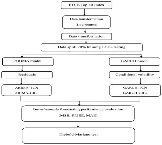
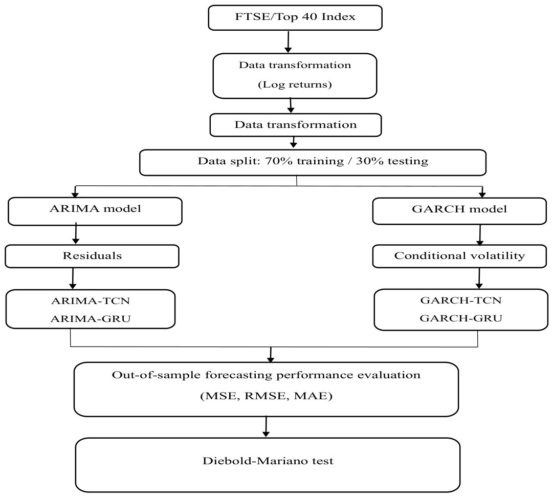
where is the average loss differential between the two models; denotes the estimated autocovariance of the loss differential at lag ; represent the truncation lag and is the number of forecasts (sample size). The methodology flowchart is presented in Figure 1.
Figure 1.
Methodology flowchart.
4. Discussion of Results
This section of the study presents the results of the data analysis, and discussions of the results obtained from the findings. The findings are presented using tables and figures. Table 1 displays the results for descriptive statistics, which summarise and explain the dataset used in the study.
Table 1.
Descriptive Statistics for the FTSE/JSE Top 40 index.
Table 1 presents the descriptive statistics for the FTSE/JSE Top 40 index and its daily log returns. The dataset contains 4159 index observations and 4158 log-return observations. The index has a mean of 53,052.01 and a median of 48,766.71, with positive skewness 0.99, indicating a right-skewed distribution. The standard deviation of 20,179.61 also indicates substantial variation in index levels.
The log returns have a mean of 0.0004 and a standard deviation of 0.0115, indicating that daily returns are centred close to zero. The returns are slightly negatively skewed −0.2838 and exhibit high kurtosis 8.6537, indicating the presence of heavy tails and extreme observations. These characteristics are typical of financial return series and provide support for applying volatility and nonlinear forecasting models.
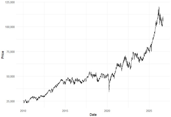
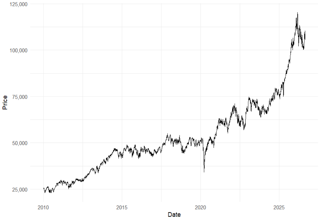
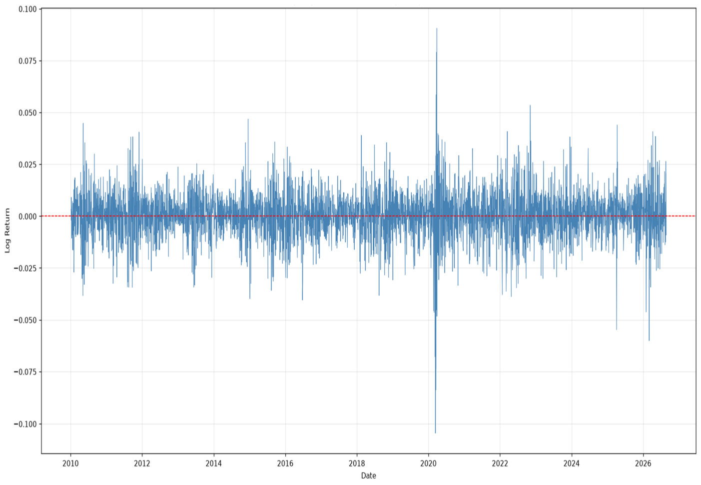
Figure 2 illustrates the daily closing values of the FTSE/JSE Top 40 index over the period from 2010 to 2026. The series exhibits pronounced time-varying behaviour, characterised by a clear upward trend and substantial price fluctuations. The index increases from around 25,000 in 2010 to approximately 50,000 by 2015, followed by periods of fluctuations between 2015 and 2020. A sharp decline is evident around early 2020, after which the index recovers and resumes an upward trajectory, reaching approximately 75,000 by 2024. The index then experiences a substantial increase during 2025 and early 2026, reaching a peak of around 120,000 before declining to approximately 100,000 by August 2026. The changing mean level and persistent upward trend provide evidence of non-stationarity in the price series. In addition, the varying magnitude of price movements suggests time-varying market dynamics. These characteristics indicate that the series requires transformation before modelling. Accordingly, the daily log-return series is used in Figure 3 to assess stationarity, serial dependence, and volatility characteristics.
Figure 2.
Graphical representation of the actual data.
Figure 3.
Daily log returns of FTSE/JSE Top 40 closing stock prices.
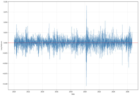
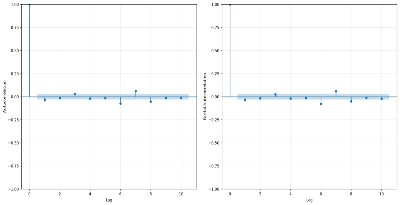
Figure 3 shows that the daily log returns fluctuate around zero, indicating a more stable mean. The series also displays periods of high and low fluctuations, suggesting changes in market volatility over time. Figure 4 presents the ACF and PACF plots of the log-return series, which are used to assess the presence of serial dependence.
Figure 4.
ACF and PACF of the daily log returns.
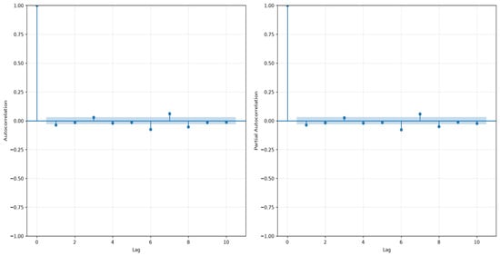
Figure 4 presents the ACF and PACF plots of the daily log-return series. Most of the lagged autocorrelations fall within the confidence intervals, indicating limited serial dependence in the log returns. Table 2 presents the results of the ARCH-LM, Ljung–Box, and Jarque–Bera tests, which further assess volatility clustering, serial correlation, and the normality of the log-return series.
Table 2.
The results for ARCH LM, Ljung–Box and JB tests.
Table 2 presents the diagnostic test results for the FTSE/JSE Top 40 log-return series. The ARCH-LM test is significant χ2 = 1021.047, p < 0.001, indicating the presence of ARCH effects and volatility clustering. The Ljung–Box test is also significant χ2 = 65.416, p < 0.001, indicating significant serial dependence in the returns. The Jarque–Bera test is significant χ2 = 5577.582, p < 0.001, rejecting the assumption of normality and indicating non-normal, heavy-tailed return behaviour. These findings motivate the use of models capable of capturing volatility dynamics and nonlinear patterns in the FTSE/JSE Top 40 series. Accordingly, the study compares traditional statistical models ARIMA and GARCH, deep learning models TCN and GRU, and hybrid models ARIMA-TCN, ARIMA-GRU, GARCH-TCN, and GARCH-GRU to identify the most effective approach for forecasting the South African equity market.
Table 3 presents the parameter estimates for the selected model fitted to the log-return series of the FTSE/JSE Top 40 index. The optimal ARIMA specification was identified using the procedure, with model selection based on the AIC. The procedure selected as the preferred specification. The estimated AR and MA coefficients represent the temporal dependence captured in the log-return series. The selected model was subsequently subjected to residual diagnostic tests to assess its adequacy for forecasting.
Table 3.
ARIMA model.
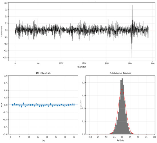
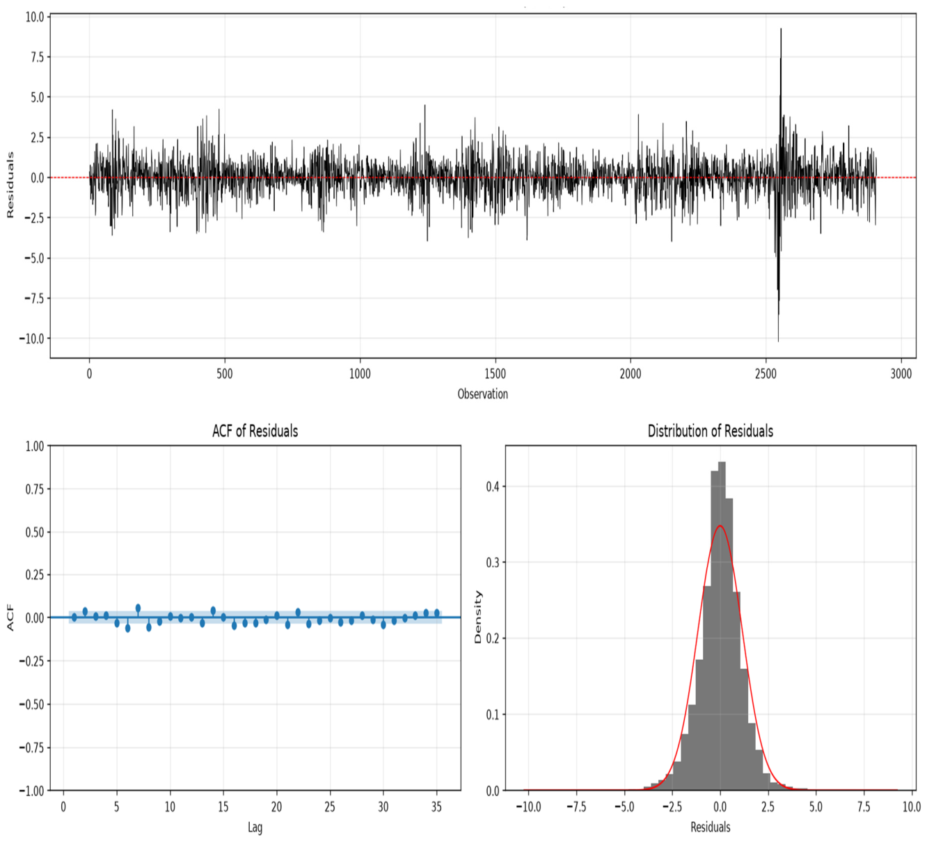
Figure 5 presents the diagnostic checks for the model. The residual time series fluctuates around zero, suggesting that the model adequately captures the underlying trend and linear dependence in the data. However, several pronounced spikes are observed, particularly towards the end of the sample, indicating the presence of extreme observations or market shocks that are not fully explained by the model. The residual ACF shows several autocorrelation coefficients outside the 95% confidence bounds, indicating that some serial correlation remains in the residuals. Nevertheless, the residual distribution departs noticeably from normality, with heavy tails and extreme observations, which are common characteristics of financial time series. Overall, the diagnostics indicate that the ) model captures a key component of the conditional mean, but some dependence and large fluctuations remain. Consequently, the study employs the GARCH model to investigate the conditional variance and capture the volatility dynamics inherent in the FTSE/JSE Top 40 index, with the results presented in Table 4.
Figure 5.
Diagnostic checks for model.
Table 4.
Results of the parameter estimates.
Table 4 presents the parameter estimates for the model fitted to the daily log returns of the FTSE/JSE Top 40 index. GARCH specifications, including , and were also estimated and compared using the AIC. Based on the model comparison, the model was selected as the preferred specification.
Table 4 further shows that the estimated ARCH coefficients α1 = 0.0681 and α2 = 0.1044) are positive and statistically significant, indicating that recent market shocks significantly influence current conditional volatility. The second-order GARCH coefficient β2 = 0.7526 is also positive and statistically significant, indicating substantial volatility persistence. However, the first-order GARCH coefficient β1 = 0.0269 is not statistically significant. The combined persistence parameter, , is close to but below unity, suggesting that volatility shocks are highly persistent but gradually dissipate over time. The model achieved an AIC value of 2.8999. Overall, the results indicate strong and persistent volatility dynamics in the FTSE/JSE Top 40 index. The residual diagnostic results of the fitted model is presented in Table 5 to assess whether the model has adequately captured the remaining conditional heteroscedasticity.
Table 5.
The results for robustness checks.
Table 5 presents the results of the residual diagnostic tests. The ARCH-LM test produced a chi-squared statistic of 10.9626 with a p-value of 0.3604, indicating no significant remaining ARCH effects in the residuals. The Ljung–Box test yielded a chi-squared statistic of 23.4498 with a p-value of 0.4364, suggesting that the residuals do not exhibit significant serial correlation and can therefore be regarded as white noise. These results indicate that the model adequately captures the volatility clustering and serial dependence in the data. However, the Jarque–Bera test produced a chi-squared statistic of 155.0452 with a p-value of <0.0000, rejecting the null hypothesis of normality. This indicates that the residuals remain non-normally distributed, reflecting the heavy-tailed characteristics and extreme movements commonly observed in financial return data. Overall, the diagnostic results support the adequacy of the model in capturing the volatility dynamics of the FTSE/JSE Top 40 index. The results for the TCN model are presented in Figure 6 and Table 6.
Figure 6.
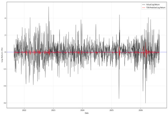
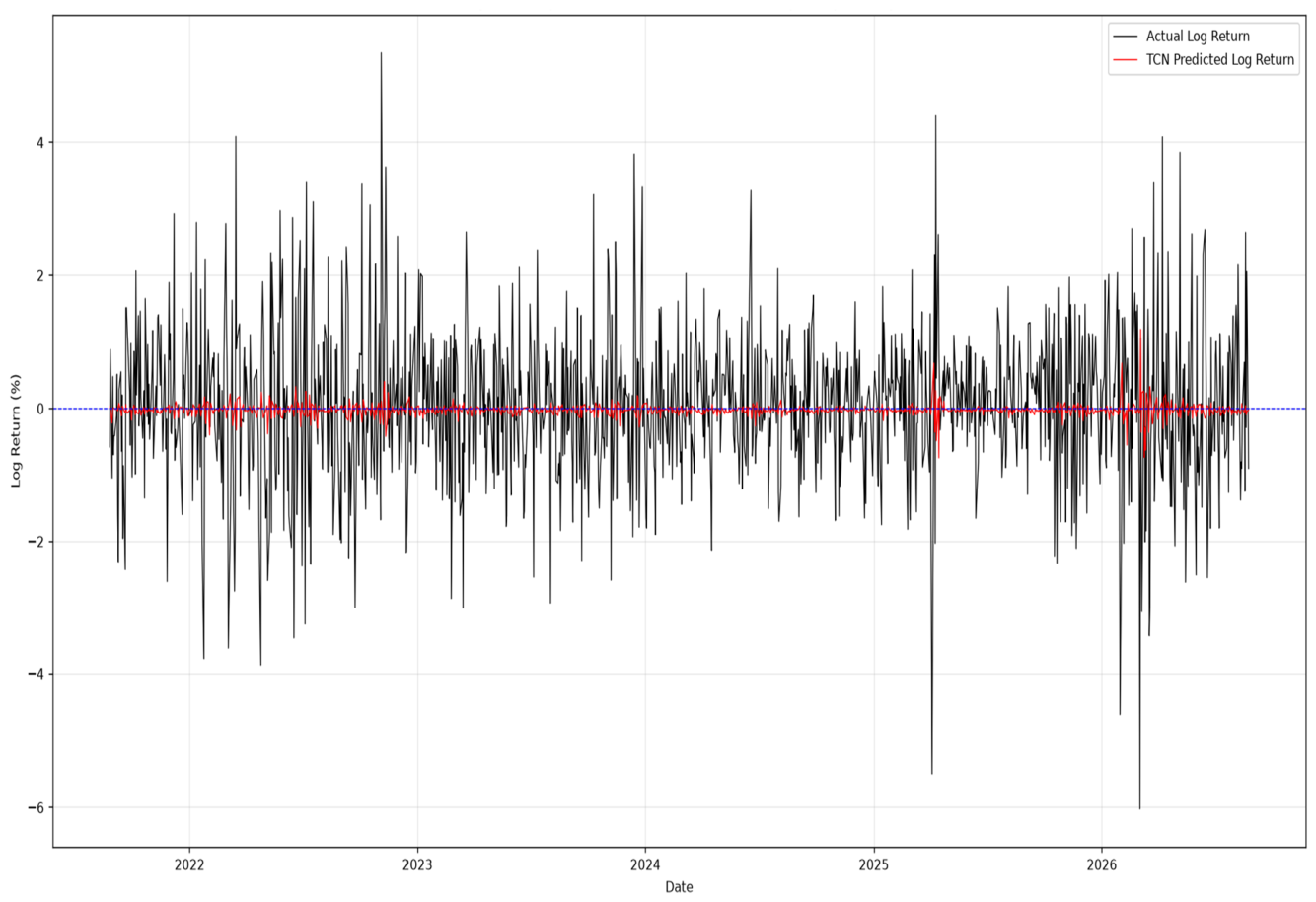
TCN rolling one-step-ahead forecast vs. actual FTSE/JSE Top 40 log returns.
Table 6.
TCN accuracy measures.
Figure 6 illustrates the rolling one-step-ahead forecasting performance of the TCN model for the FTSE/JSE Top 40 log returns. The model uses 3 temporal convolutional layers with 32, 64, and 32 filters, respectively, a kernel size of 3, and dilation factors of 1, 2, and 4 to capture temporal dependencies across different time scales. Residual connections are used between the temporal blocks, with a 10-day input window and a batch size of 32. The model is trained for 50 epochs using the Adam optimiser with a learning rate of 0.001 and a dropout rate of 0.2.
As shown in Figure 6, the actual log returns exhibit substantial short-term fluctuations and volatility throughout the test period, whereas the TCN forecasts remain close to zero and display less variation. This indicates that the model captures the general central tendency of the return series but has limited ability to reproduce the magnitude of individual return movements and volatility spikes.
Table 6 presents the accuracy measures of the TCN model for forecasting the FTSE/JSE Top 40 log returns. The model recorded an RMSE of 1.1543, an MSE of 1.3324, and an MAE of 0.8568. These results indicate the forecasting error associated with the TCN model over the test period, with the MAE showing that the average absolute forecasting error was approximately 0.8568% in log-return terms. These findings are consistent with those of [11], who reported that TCN models achieve high forecasting accuracy by effectively learning long-range temporal dependencies while maintaining stable training performance. The results for GRU are presented in Figure 7 and Table 7.
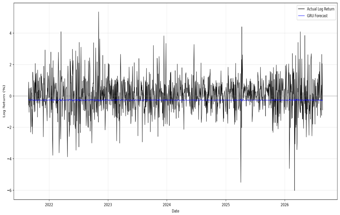
Figure 7.
GRU rolling one-step-ahead forecast vs. actual FTSE/JSE Top 40 log returns.
Table 7.
GRU accuracy measures.
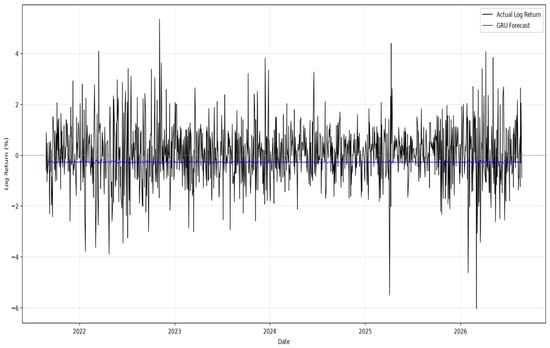
Figure 7 illustrates the rolling one-step-ahead forecasting performance of the GRU model for the FTSE/JSE Top 40 log returns. The GRU architecture consists of two recurrent layers with 64 hidden units, designed to capture temporal dependencies in the return series. A 10-day input window and a batch size of 32 are used. The model is trained for 50 epochs using the Adam optimiser with a learning rate of 0.001 and a dropout rate of 0.2. Overall, the results indicate that the GRU provides limited forecasting accuracy for the highly volatile FTSE/JSE Top 40 log returns.
Table 7 shows that the model achieved an MSE of 1.4161, RMSE of 1.1900, and MAE of 0.8978 on the test set. The rolling one-step-ahead forecasts indicate that the GRU captures some of the short-term temporal structure in the FTSE/JSE Top 40 log-return series; however, the small variation in the predicted returns compared with the observed returns suggests that the model has limited ability to capture the magnitude of larger movements. Overall, the results indicate that the GRU provides limited forecasting accuracy for the highly volatile FTSE/JSE Top 40 log returns. Figure 8 represents the actual vs. predicted forecasts of the ARIMA and GARCH-based hybrid models.
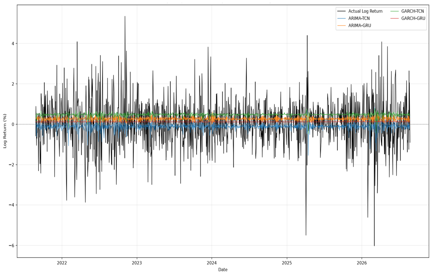
Figure 8.
The actual vs. predicted forecasts of the ARIMA and GARCH-based hybrid models.
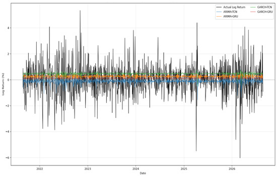
Figure 8 presents the actual FTSE/JSE Top 40 log returns alongside the forecasts generated by the four hybrid models. The actual return series exhibits substantial volatility and several pronounced positive and negative shocks, whereas the model forecasts remain considerably smoother and are concentrated around the conditional mean of the return process. This behaviour is consistent with the difficulty of predicting individual financial return innovations, which are characterised by substantial noise and time-varying volatility. Among the hybrid models, GARCH-GRU generally produces forecasts at a slightly higher level than the other models, while GARCH-TCN displays a somewhat distinct forecast profile. However, the visual differences between the models are relatively small compared with the magnitude of the realised returns. Therefore, the figure provides qualitative evidence of forecast behaviour but does not, by itself, establish predictive superiority. Forecasting performance was assessed using two complementary approaches: benchmarking against the Naïve model and formal statistical testing using the DM test. The Naïve model served as the benchmark against which all competing forecasting models were evaluated, providing a baseline for determining whether the models offered improvements over a simple forecasting strategy.
Table 8 compares the forecasting performance of the competing models against the Naïve benchmark using MSE, RMSE, and MAE. The Naïve benchmark, which uses the previous observed log return as the one-step-ahead forecast, records an MSE of 2.6342, RMSE of 1.6230, and MAE of 1.2351, providing a relatively demanding benchmark for evaluating the forecasting models. All the competing models substantially improve upon the Naïve benchmark across all three error measures. The GARCH-GRU model achieves the best overall forecasting performance, recording the lowest MSE of 1.3216, RMSE of 1.1496, and MAE of 0.8552, representing a substantial reduction in forecasting error relative to the Naïve benchmark. The standalone GARCH model performs very similarly, with an MSE of 1.3223, RMSE of 1.1499, and MAE of 0.8566, while the TCN records an MSE of 1.3324, RMSE of 1.1543, and MAE of 0.8568. The ARIMA-TCN and ARIMA-GRU models also outperform the Naïve benchmark, with MSE values of 1.3509 and 1.3589, respectively. The standalone ARIMA model records an MSE of 1.3652, RMSE of 1.1684, and MAE of 0.8691, whereas the GRU records an MSE of 1.4161, RMSE of 1.1900, and MAE of 0.8978. The GARCH-TCN model records the highest error among the competing models, with an MSE of 1.5016, RMSE of 1.2254, and MAE of 0.9231, although it still substantially outperforms the Naïve benchmark.
Table 8.
Forecasting performance of the competing models against the Naïve benchmark.
Overall, the results demonstrate that incorporating time-series dynamics and volatility information provides considerably greater predictive accuracy than simply using the previous observed return. In particular, the superior performance of GARCH-GRU suggests that combining conditional volatility modelling with the GRU’s ability to capture nonlinear temporal dependencies provides an effective approach for forecasting FTSE/JSE Top 40 log returns. The superior performance of the GARCH-GRU model is consistent with the findings of [11], who reported that hybrid GARCH-deep learning models outperform standalone statistical and deep learning approaches in forecasting stock prices by effectively capturing both volatility persistence and nonlinear market behaviour. Similarly, ref. [13] found that hybrid statistical–deep learning models generate more accurate and robust forecasts than individual modelling approaches because they simultaneously account for conditional heteroscedasticity and complex temporal dependencies. Table 9 present the results for GARCH-GRU vs. using the DM test.
Table 9.
DM test results.
The DM test produced a DM statistic of 0.9495 and a p-value of 0.3424. Since the p-value is greater than the significance level 0.05, the null hypothesis of equal predictive accuracy is not rejected. Therefore, although the forecasting results may show that GARCH-GRU performs better than in terms of MSE, RMSE, or MAE, the difference is not statistically significant according to the DM test. In other words, the results do not provide sufficient statistical evidence to conclude that GARCH-GRU has superior predictive accuracy to . The observed improvement in the point forecast metrics may therefore reflect sampling variation rather than a statistically reliable difference in forecasting performance.
5. Conclusions and Recommendations
This study evaluated the forecasting performance of traditional econometric models, deep learning models, and hybrid forecasting frameworks for the FTSE/JSE Top 40 index. Specifically, the study compared ARIMA and GARCH models with TCN and GRU architectures, together with four hybrid models: ARIMA-TCN, ARIMA-GRU, GARCH-TCN, and GARCH-GRU. The objective was to determine whether combining traditional statistical modelling with deep learning techniques could improve out-of-sample forecasting accuracy in the South African equity market. The empirical results showed that model performance differs across the forecasting approaches, with the hybrid models producing competitive results relative to the standalone models. The ARIMA and GARCH models provided a statistical representation of the dependence and volatility characteristics of the return series, while the TCN and GRU models are designed to capture nonlinear temporal relationships. Among the standalone deep learning models, the TCN produced lower MSE, RMSE, and MAE than the GRU, indicating stronger forecasting performance for the test-period log returns. Nevertheless, the GRU remained competitive, particularly when combined with GARCH volatility information. This is consistent with [6,7], who found that TCN-based architectures can provide an effective balance between predictive performance and computational efficiency in financial time-series forecasting.
The hybrid results provide further evidence that combining complementary modelling approaches can provide competitive forecasting performance. The GARCH-GRU model recorded an MSE of 1.3216, RMSE of 1.1496, and MAE of 0.8552, while the standalone model produced very similar values of 1.3223, 1.1499, and 0.8566, respectively. The small differences between the two models indicate that their forecasting performance is very similar based on the point forecast measures. Although the GARCH-GRU model records marginally lower errors, the results do not indicate a meaningful forecasting advantage over . The performance of these models highlights the relevance of incorporating volatility information when forecasting financial return dynamics. This finding is supported by [11], who demonstrated the value of combining GARCH-based volatility modelling with deep learning techniques. The findings are also consistent with [5,10,12], who reported that integrating traditional statistical models with deep learning architectures can exploit the complementary strengths of statistical and nonlinear forecasting methods.
The comparison with the Naïve benchmark provides further evidence of the value of the forecasting approaches considered in this study. The Naïve benchmark recorded an MSE of 2.6342, RMSE of 1.6230, and MAE of 1.2351, which were substantially higher than those of all the competing models. This indicates that all the models considered in the study provide considerably greater forecasting accuracy than simply using the previous observed log return as the one-step-ahead forecast. The results therefore demonstrate that incorporating time-series dependence, volatility dynamics, and nonlinear relationships provides a substantial improvement over the Naïve forecasting approach. In particular, the close performance of GARCH-GRU and , combined with their substantial improvement over the Naïve benchmark, suggests that volatility-based modelling is particularly relevant for forecasting FTSE/JSE Top 40 log returns.
The DM test revealed that there is no statistically significant difference in predictive accuracy between GARCH-GRU and . The small differences observed in their MSE, RMSE, and MAE values should consequently not be interpreted as evidence that one model is statistically superior to the other. Instead, the findings indicate that GARCH-GRU and provide statistically comparable forecasting performance for the FTSE/JSE Top 40 log returns.
The results also highlight that hybridisation does not automatically guarantee improved forecasting performance. For example, the GARCH-TCN model recorded the highest MSE RMSE and MAE among the competing models, whereas GARCH-GRU and produced substantially lower errors. Similarly, the ARIMA-based hybrid models did not consistently outperform their standalone counterparts. These findings indicate that the effectiveness of a hybrid framework depends not only on the inclusion of statistical information, but also on how that information interacts with the underlying neural network architecture. Thus, the results provide a more nuanced assessment of hybrid forecasting rather than if greater model complexity necessarily produces superior forecasts.
The performance of the GARCH-based models further highlights the relevance of volatility dynamics in financial forecasting. Financial return series commonly exhibit volatility clustering and time-varying variance, which may not be fully captured by models focused solely on temporal or nonlinear relationships. Incorporating GARCH-generated volatility information provides an additional representation of these characteristics, while the neural network component can model more complex temporal relationships. The comparable performance of GARCH-GRU and , together with their substantial improvement over the Naïve benchmark, suggests that modelling conditional volatility provides an important contribution to forecasting performance. This finding is consistent with [13], who emphasised the potential of hybrid statistical–deep learning models to provide robust forecasting frameworks, and with [4], who argued that hybrid approaches can benefit from combining complementary modelling paradigms.
This study contributes to the financial forecasting literature in three main respects. First, it provides a comparative evaluation of traditional statistical, deep learning, and hybrid forecasting models using data from the South African equity market. Second, it extends the application of hybrid statistical–deep learning approaches to an emerging African market, where empirical evidence remains comparatively limited. Third, the study provides a systematic comparison based on out-of-sample MSE, RMSE, and MAE, supplemented by the DM test, allowing forecasting performance to be assessed using both error-based and statistical measures.
The findings also have practical implications for financial forecasting and decision support. The results demonstrate that the forecasting models considered in this study provide substantial improvements over the Naïve benchmark. In particular, the comparable performance of GARCH-GRU and suggests that both approaches can provide useful forecasts of FTSE/JSE Top 40 log returns. Importantly, the DM test indicates that the additional complexity of the GARCH-GRU framework does not produce a statistically significant improvement over the standalone model. This highlights the importance of considering statistical significance alongside conventional forecasting error measures when selecting forecasting models. Such forecasts may support portfolio management, risk assessment, and investment decision-making. However, the results should not be interpreted as implying that one model will always be superior under all market conditions. Forecasting performance may vary across market regimes, datasets, forecasting horizons, and asset classes. Several limitations should also be acknowledged. The analysis focuses on the FTSE/JSE Top 40 index and primarily uses historical market information. Variables such as macroeconomic conditions, investor sentiment, trading volume, and firm-specific information are therefore not explicitly incorporated. In addition, although several statistical, deep learning, and hybrid architectures were considered, more recent attention-based and Transformer-based approaches were outside the scope of the present study.
Future research could extend the framework by incorporating macroeconomic indicators, technical indicators, news sentiment, trading information, and other alternative data sources. Attention-based and Transformer architectures could also be investigated to determine whether they provide additional forecasting benefits [15,16]. Further comparisons across different African and international equity markets would provide additional evidence regarding the robustness and generalisability of the findings.
Overall, the findings indicate that the forecasting models considered in this study substantially outperform the Naïve benchmark, demonstrating the value of incorporating time-series and volatility dynamics when forecasting FTSE/JSE Top 40 log returns. Although GARCH-GRU records slightly lower MSE, RMSE, and MAE values than , the DM test indicates that this difference is not statistically significant. Therefore, GARCH-GRU and should be regarded as having statistically comparable forecasting performance rather than one being superior to the other. The findings consequently suggest that volatility-based approaches provide competitive forecasting performance, while the lack of a significant difference between the GARCH-GRU and models demonstrate that increased model complexity does not necessarily translate into statistically significant forecasting improvements.
Author Contributions
Conceptualization, J.T.T., P.M.L.S., S.N. and D.M.; methodology, J.T.T.; formal analysis, P.M.L.S.; data curation, J.T.T.; writing—original draft, J.T.T., P.M.L.S., S.N. and D.M.; writing—review & editing, J.T.T. and P.M.L.S. All authors have read and agreed to the published version of the manuscript.
Funding
This research received no external funding.
Data Availability Statement
The study employed secondary data obtained from IRESS. The data is also publicly available from Investing.com (South Africa Top 40 Index (JTOPI)—Investing.com ZA, https://za.investing.com/indices/ftse-jse-top-40 (accessed on 24 August 2026)).
Conflicts of Interest
The authors declare no conflicts of interest.
Abbreviations
The following abbreviations are used in this manuscript:
| ACF | Autocorrelation Function |
| AI | Artificial Intelligence |
| AIC | Akaike Information Criterion |
| AR | Autoregressive |
| ARIMA | Autoregressive Integrated Moving Average |
| BiLSTM | Bidirectional LSTM |
| DM | Diebold–Mariano |
| EDA | Exploratory data analysis |
| GARCH | Generalised Autoregressive Conditional Heteroskedasticity |
| LSTM | Long Short-Term Memory |
| GRU | Gated Recurrent Unit |
| MA | Moving Average |
| MAE | Mean Absolute Error |
| ML | Machine Learning |
| MLE | Maximum Likelihood Estimation |
| MSE | Mean Squared Error |
| PACF | Partial Autocorrelation Function |
| RMSE | Root Mean Squared Error |
| RNN | Recurrent Neural Network |
| TCN | Temporal Convolutional Network |
References
- Box, G.; Jenkins, G.M. Analysis: Forecasting and Control; Holden-Day: San Francisco, CA, USA, 1976; Volume 10. [Google Scholar]
- Bollerslev, T. Generalized Autoregressive Conditional Heteroskedasticity. J. Econ. 1986, 31, 307–327. [Google Scholar] [CrossRef] [Scilit]
- Mehtarizadeh, H.; Mansouri, N.; Mohammad Hasani Zade, B.; Hosseini, M.M. Stock Price Prediction with SCA-LSTM Network and Statistical Model ARIMA-GARCH. J. Supercomput. 2025, 81, 366. [Google Scholar] [CrossRef] [Scilit]
- Cheng, C.; Li, C.; Weng, G. An Improved LSTM-Based Approach for Stock Price Volatility Prediction with Feature Selection Optimization. Artif. Intell. Mach. Learn. Rev. 2023, 4, 1–15. [Google Scholar]
- Osman, E.G.A. Integrating Deep Learning and Econometrics for Stock Price Prediction: An Empirical Study of LSTM and Traditional Time Series Models. Mach. Learn. Appl. 2025, 22, 100730. [Google Scholar] [CrossRef] [Scilit]
- Makridakis, S.; Spiliotis, E.; Assimakopoulos, V.; Semenoglou, A.-A.; Mulder, G.; Nikolopoulos, K. Statistical, Machine Learning and Deep Learning Forecasting Methods: Comparisons and Ways Forward. J. Oper. Res. Soc. 2023, 74, 840–859. [Google Scholar] [CrossRef] [Scilit]
- Si, Y.; Nadarajah, S.; Zhang, Z.; Xu, C. Modeling Opening Price Spread of Shanghai Composite Index Based on ARIMA-GRU/LSTM Hybrid Model. PLoS ONE 2024, 19, e0299164. [Google Scholar] [CrossRef] [Scilit] [PubMed]
- Pirani, M.; Thakkar, P.; Jivrani, P.; Bohara, M.H.; Garg, D. A Comparative Analysis of ARIMA, GRU, LSTM and BiLSTM on Financial Time Series Forecasting. In Proceedings of the 2022 IEEE International Conference on Distributed Computing and Electrical Circuits and Electronics (ICDCECE); IEEE: New York, NY, USA, 2022; pp. 1–6. [Google Scholar]
- Wang, Q. Stock Prediction under GRU, LSTM and GNN. In Proceedings of the 2024 IEEE 2nd International Conference on Image Processing and Computer Applications (ICIPCA); IEEE: New York, NY, USA, 2024; pp. 460–464. [Google Scholar]
- Xiao, J.; Deng, T.; Bi, S. Comparative Analysis of LSTM, GRU, and Transformer Models for Stock Price Prediction. In Proceedings of the International Conference on Digital Economy, Blockchain and Artificial Intelligence, Guangzhou, China, 23–25 August 2024; ACM: New York, NY, USA, 2024; pp. 103–108. [Google Scholar]
- Harefa, V.N.; Saepudin, D. Prediction of Stock Price Movements on the Indonesia Stock Exchange (IDX) Based on Company Fundamental Ratios Using the Temporal Convolutional Network (TCN) Method. In Proceedings of the 2025 International Conference on Information and Communication Technology (ICoICT); IEEE: New York, NY, USA, 2025; pp. 1–6. [Google Scholar]
- Shabbeer, M.; Pravalika, M.; Pitchai, R.; Madhubabu, C. Arima-Gru Hybrid Model for Stock Exchange Forecast. In Proceedings of the 2023 9th International Conference on Smart Computing and Communications (ICSCC); IEEE: New York, NY, USA, 2023; pp. 41–44. [Google Scholar]
- Mutinda, J.K.; Langat, A.K. Stock Price Prediction Using Combined GARCH-AI Models. Sci. Afr. 2024, 26, e02374. [Google Scholar] [CrossRef] [Scilit]
- Chen, X.; Zheng, X.; Liu, B.-X. Stock Price Forecasting Model Based on ARIMA-TCN. In Proceedings of the 2025 8th World Conference on Computing and Communication Technologies (WCCCT); IEEE: New York, NY, USA, 2025; pp. 425–431. [Google Scholar]
- Nwanegbo, I.M.; Daniel, J.; Pauline, A. Hybrid Deep Learning and Econometric Models for Forecasting Equity Returns. Int. J. Financ. Manag. Econ. 2024, 7, 833–840. [Google Scholar] [CrossRef] [Scilit]
- Lipton, Z.C. The Mythos of Model Interpretability: In Machine Learning, the Concept of Interpretability Is Both Important and Slippery. Queue 2018, 16, 31–57. [Google Scholar] [CrossRef] [Scilit]
- Nhlapho, W.; Atemkeng, M.; Ndogmo, J.-C. An Attention-Guided Hybrid Statistical and Deep Learning Modeling for Enhanced Time Series Forecasting: A Case Study of South African Telecommunication Companies. Sci. Afr. 2025, 30, e02950. [Google Scholar] [CrossRef] [Scilit]
- Wang, P.; Wang, Z. Stock Prediction Based on TCN-ARIMA-GARCH Model with Intelligent Optimization Algorithm. In Proceedings of the 2024 International Conference on Digital Society and Artificial Intelligence, Qingdao China, 24 May 2024; ACM: New York, NY, USA, 2024; pp. 225–232. [Google Scholar]
- Engle, R.F. Autoregressive Conditional Heteroscedasticity with Estimates of the Variance of United Kingdom Inflation. Econom. J. Econom. Soc. 1982, 50, 987–1007. [Google Scholar] [CrossRef] [Scilit]
- Ljung, G.M.; Box, G.E. On a Measure of Lack of Fit in Time Series Models. Biometrika 1978, 65, 297–303. [Google Scholar] [CrossRef]
- Jarque, C.M.; Bera, A.K. Efficient Tests for Normality, Homoscedasticity and Serial Independence of Regression Residuals. Econ. Lett. 1980, 6, 255–259. [Google Scholar] [CrossRef] [Scilit]
- Tsoku, J.T.; Metsileng, D.; Botlhoko, T. Modelling South African Gold Sales Using SARIMA, GARCH and Neural Networks. Mathematics 2026, 14, 1289. [Google Scholar] [CrossRef] [Scilit]
- Bowerman, B.L.; O’Connell, R.T.; Koehler, A.B. Forecasting, Time Series, and Regression: An Applied Approach; Duxbury Press: London, UK, 2005. [Google Scholar]
- Lara-Benítez, P.; Carranza-García, M.; Luna-Romera, J.M.; Riquelme, J.C. Temporal Convolutional Networks Applied to Energy-Related Time Series Forecasting. Appl. Sci. 2020, 10, 2322. [Google Scholar] [CrossRef] [Scilit]
- Bai, S.; Kolter, J.Z.; Koltun, V. An Empirical Evaluation of Generic Convolutional and Recurrent Networks for Sequence Modeling. arXiv 2018, arXiv:1803.01271. [Google Scholar]
- Zanghieri, M.; Benatti, S.; Burrello, A.; Kartsch, V.; Conti, F.; Benini, L. Robust Real-Time Embedded EMG Recognition Framework Using Temporal Convolutional Networks on a Multicore IoT Processor. IEEE Trans. Biomed. Circuits Syst. 2019, 14, 244–256. [Google Scholar] [CrossRef] [Scilit] [PubMed]
- Cho, K.; Van Merriënboer, B.; Bahdanau, D.; Bengio, Y. On the Properties of Neural Machine Translation: Encoder–Decoder Approaches. In Proceedings of the SSST-8, Eighth Workshop on Syntax, Semantics and Structure in Statistical Translation; Association for Computational Linguistics: Stroudsburg, PA, USA, 2014; pp. 103–111. [Google Scholar]
- Bahdanau, D.; Cho, K.; Bengio, Y. Neural Machine Translation by Jointly Learning to Align and Translate. arXiv 2014, arXiv:14090473. [Google Scholar]
- Diebold, F.X.; Mariano, R.S. Comparing Predictive Accuracy. J. Bus. Econ. Stat. 2002, 20, 134–144. [Google Scholar] [CrossRef] [Scilit]

Disclaimer/Publisher’s Note: The statements, opinions and data contained in all publications are solely those of the individual author(s) and contributor(s) and not of MDPI and/or the editor(s). MDPI and/or the editor(s) disclaim responsibility for any injury to people or property resulting from any ideas, methods, instructions or products referred to in the content. |
© 2026 by the authors. Licensee MDPI, Basel, Switzerland. This article is an open access article distributed under the terms and conditions of the Creative Commons Attribution (CC BY) license.