Pooling Beats Structure on Short Annual Panels: Parameter Sharing and the Forecast Accuracy of Evolutionary Models for Compositional Time Series

Highlights

What are the main findings?

• Sharing parameters across countries reduces forecast error by 15.3% to 27.8% across three Eurostat panels, an effect larger than the gap between the best structural model and the best statistical benchmark.
• Replicator–mutator structure does not by itself improve accuracy; it ties the random walk with drift, which it nests as a special case, to educational attainment and loses to a no-change forecast on municipal waste routes. Pooled kernel and neural benchmarks finish mid-field on every panel.

What are the implications of the main findings?

• On short annual panels of official statistics, estimating evolutionary models country by country is the single choice most damaging to out-of-sample accuracy; a validation-selected parameter-sharing regime corrects it, and a simulation grid shows that the gain hinges on limited cross-country parameter heterogeneity.
• The shrinkage weight and the mutation rate are tuning parameters rather than structural constants and should be selected by walk-forward optimisation inside the training window; the estimated congestion parameters keep their economic reading, increasing returns in attainment and congestion in waste routes.

Abstract

Many economic time series are compositions: educational attainment shares, waste treatment routes, energy mixes, and sectoral employment. Forecasters usually move such series to log-ratio coordinates and apply generic methods that impose no economic restriction on how the parts move. Evolutionary game theory supplies one: replicator dynamics make the growth rate of a share proportional to its payoff advantage, which is the logic of imitation, diffusion and congestion that economics itself uses to explain why shares move. We turn that restriction into a forecast function with $K+1$ parameters for a $K$-part composition; estimate it under three parameter-sharing regimes, namely country-specific, fully pooled and validation-shrunk; and race it against classical log-ratio benchmarks, a non-evolutionary Dirichlet comparator and two pooled machine-learning benchmarks in an expanding-window, rolling-origin design on three Eurostat panels. The evolutionary restriction does not buy accuracy: its best specification ties the random walk with drift on educational attainment and loses to persistence on municipal waste routes. What moves accuracy is the sharing regime. Moving from country-specific estimation to the best sharing regime cuts the mean absolute scaled error by 27.8% on attainment and by 15.3% to 19.8% on the waste panels, more than the gap between the best structural and the best statistical model, and the same ordering reappears in the Dirichlet family. The estimated congestion parameters carry the economics the restriction was built for, increasing returns in attainment and congestion in waste routes, while a simulation grid shows the sharing gain reversing once cross-country heterogeneity is appreciable. We close with a walk-forward procedure for tuning the shrinkage weight and the mutation rate.

1. Introduction

A large share of the quantities that economists forecast are not levels but shares. The educational composition of the working-age population, the split of municipal waste across treatment routes, the fuel mix of an electricity system, the distribution of employment across contract types: in each case the object of interest is a vector of non-negative parts that sums to one. Such vectors live on the unit simplex, and forecasting them with methods designed for unconstrained series risks predictions that are negative, that fail to add up, or that drift outside the feasible region at long horizons.

The standard response, following Aitchison [1,2], is to move to log-ratio coordinates, forecast there with a generic method, and map the result back. This solves the coherence problem completely and cheaply. What it does not do is impose any economic content. A vector autoregression in log-ratio coordinates treats the composition as an arbitrary multivariate process; nothing in its structure says that a part should grow when the activity it represents is doing comparatively well.

Economics has a natural candidate for exactly that restriction. Replicator dynamics, introduced by Taylor and Jonker [3] and developed into the standard apparatus of evolutionary game theory by Hofbauer and Sigmund [4], Weibull [5] and Sandholm [6], make the growth rate of a share proportional to the gap between its payoff and the population average payoff. Its behavioural microfoundations are well understood: it arises from imitation of successful others under bounded rationality [7] and from payoff-monotone revision protocols more generally [6]. Adding mutation, in the sense of Nowak, Komarova and Niyogi [8] and Komarova [9], introduces a small flow toward strategies that are not currently doing well, which can be read as experimentation, entry, or simply the failure of imitation to be perfect. Section 2 shows that this restriction is not an import from biology: the logistic diffusion curve, the substitution model of technological change and the congestion game are all special cases of it, and economics has been using them to explain moving shares for seventy years.

Why this matters is a question about practice rather than about theory. Evolutionary and replicator specifications are now routinely fitted to shares taken from official statistics, and the standard reporting pattern in that applied literature is an in-sample fit, estimated unit by unit, with the model judged by how closely the fitted path tracks the observed one. Nothing in that pattern tells a user whether the restriction helps on data that have not yet been seen, which is the only sense in which a forecasting model earns its keep, and nothing tells the user whether the effort spent on specifying payoffs would be better spent elsewhere. Two questions are therefore open, and the paper is organised around them. First, does an economic restriction on how shares move buy out-of-sample accuracy against the generic transformations that applied compositional forecasting actually uses? Second, if it does not, where does accuracy in this data environment come from instead? The answer to the second question is what makes the answer to the first useful, because it identifies the design margin a practitioner can still move.

We treat the question as a forecasting question, with a rolling-origin design, a panel of benchmarks, scale-free losses and formal tests of equal predictive ability. The answer is not the one the framing invites. The restriction does not pay for itself in accuracy: its best specification ties the random walk with drift on educational attainment, which turns out to be the special case of the evolutionary map with no frequency dependence and no mutation, and it loses to a no-change forecast on municipal waste routes. What pays is parameter sharing. Across three Eurostat panels, the spread within the structural family generated purely by how parameters are shared across countries is 18.1% to 38.5% in mean absolute scaled error, whereas the gap between the best structural specification and the best benchmark is 1.3% on one panel and 11.5% to 13.1% on the others. Moving from country-specific estimation to the best sharing regime reduces error by 27.8% on attainment and by 15.3% and 19.8% on the two waste panels, and the same ordering reappears when a non-evolutionary Dirichlet transition model is estimated under identical regimes.

It is worth saying plainly what is new here and what is not. Replicator–mutator dynamics, parameter pooling, shrinkage and the bias-variance trade-off that governs them are all established, and this paper introduces none of them. What it contributes is the controlled comparison itself: an economic restriction, a non-evolutionary simplex-native likelihood model and a set of classical log-ratio benchmarks are estimated under identical pooling regimes, at identical rolling origins, under identical losses and with identical treatment of zero parts, so that the model-class margin and the parameter-sharing margin are measured on one scale and can be read off one table. That comparison does not appear to have been made for compositional time series, and it is what allows the ordering claim to be stated at all. The claim is bounded: a simulation grid shows the ordering reversing once cross-country parameter heterogeneity is appreciable, so the result is a statement about data environments in which estimation uncertainty dominates heterogeneity, which is where short annual official panels appear to live.

The paper is organised so that the economics comes first and the technicalities last. Section 2 explains why an evolutionary restriction makes sense for compositional forecasts and gives three theoretical examples. Section 3 states the forecast function in a single equation, places the benchmarks in the same notation, defines the sharing regimes and describes the data and the evaluation protocol. Section 4 reports one coherent set of results and reads it through economic intuition. Section 5 places the result at the intersection of the economics and the forecasting literature and states its scope. Section 6 proposes a walk-forward procedure for tuning the parameters that the evidence identifies as tuning devices. Section 7 concludes. Appendix A collects the simplex geometry, the stability analysis, the estimation and benchmark details, the inferential procedures and the Monte Carlo evidence; the Supplementary Materials hold the horizon-by-horizon accuracy tables, the win-rate analysis, the estimated parameters and the robustness checks.

2. Why an Evolutionary Restriction Makes Economic Sense

2.1. What the Restriction Encodes

Let $x_t=\left(x_{1,t},\dots ,x_{K,t}\right)$ be the shares of $K$ alternatives at date $t$. The replicator restriction says that the share of alternative $k$ grows between $t$ and $t+1$ in proportion to how much better it pays than the population average, and the mutator term says that a small fraction of every share is reallocated uniformly regardless of payoff. Three economic readings of this restriction are standard, and each of them is a reason to expect it to describe the compositions that official statistics report.

The first reading is imitation. Schlag [7] showed that a population of boundedly rational agents who sample one other agent and switch to that agent’s alternative with a probability proportional to the payoff difference generates replicator dynamics in the large-population limit; Fudenberg and Levine [10] and Young [11] develop the same idea into a theory of learning in populations, and Sandholm [6] shows that any payoff-monotone revision protocol produces dynamics of the replicator class. When households choose between attainment levels, or firms and municipalities between disposal routes, the relevant decision-makers observe the outcomes of others and move toward what works, and imitation of the successful is the mechanism through which aggregate shares move.

The second reading is selection among routines. Nelson and Winter [12] built evolutionary economics on the observation that the market share of a technique or a firm grows with its relative profitability, so that the composition of an industry is the outcome of a selection process rather than of a representative optimiser. The replicator equation is the reduced form of that process: the growth rate of a share equals its payoff advantage, with no agent required to know the payoffs of alternatives it does not currently use.

The third reading is diffusion. With two alternatives and a constant payoff gap $\delta$, the replicator restriction implies that the log-odds of the two shares grows linearly, $\mathrm{l}\mathrm{n}\left(x_{1,t+1}/x_{2,t+1}\right)=\mathrm{l}\mathrm{n}\left(x_{1,t}/x_{2,t}\right)+\delta$, which is the logistic curve. Griliches [13] fitted exactly this curve to the diffusion of hybrid corn across American states and read its slope as the profitability of adoption; Fisher and Pry [14] proposed the same linear log-odds law as a general model of technological substitution and used it to forecast the replacement of one technology by another. Both are replicator dynamics under another name, and both have been forecasting devices from the start. The $K$-part map used in this paper is their multi-alternative generalisation with two additions: a congestion term that lets the payoff of an alternative depend on how many already use it, and a mutation term that keeps every alternative alive.

The congestion term is where the economics of the composition is encoded. Payoffs are linear in the composition with an alternative-specific intercept and a common congestion parameter, ${\pi }_k\left(x\right)={\alpha }_k-\gamma x_k$. A positive $\gamma$ means that an alternative becomes less attractive the more of the population uses it, which is congestion, crowding, or diminishing returns to a route, and it makes an interior rest point of the map locally stable, as Appendix A.2 shows in closed form. A negative $\gamma$ means increasing returns, so that adoption is self-reinforcing: this is the lock-in mechanism of Arthur [15], under which historical accident can select among several stable long-run compositions, and it renders the interior rest point unstable and moves the attractors toward the faces of the simplex. The sign of a single parameter therefore separates two families of economic stories, and Section 4 shows that the data sort the panels between them in the way the stories predict.

2.2. Three Theoretical Examples

The first example is educational attainment. Consider the working-age population sorted into low, medium and tertiary attainment. If the payoff to a level rose only with its scarcity, the composition would settle at an interior rest point, and the share of the tertiary level would stop growing once its wage premium was competed away. The theory of directed technical change says otherwise: Acemoglu [16] shows that a larger supply of skilled workers enlarges the market for skill-complementary technologies and can raise rather than lower the skill premium, so that the payoff to an attainment level increases with the share that already holds it. Peer effects in schooling and the co-evolution of attainment with the occupational structure that rewards it point the same way. In the notation of the map, this is $\gamma <0$: the attainment composition should trend monotonically toward the tertiary corner along an S-shaped path, and the estimated congestion parameter on the attainment panel should be negative. Section 4.2 reports that it is negative for 23 of 33 countries.

The second example is municipal waste. Treated waste is split across recycling, incineration and landfill. Each route has a marginal cost that rises with the load it carries: recycling capacity is limited by sorting and reprocessing plants, incineration by furnace capacity, landfill by remaining volume and by gate fees and taxes that increase with use. A municipality that observes the marginal cost of each route directs waste to the cheapest one at the margin, so the share of a route grows when its cost is below the average, which is the replicator restriction with $\gamma >0$. The rest point of the map is the route mix at which marginal costs are equalised across the routes in use, the condition familiar from congestion games and traffic assignment, and policy shocks such as a landfill tax enter as shifts in the intercepts ${\alpha }_k$. The estimated congestion parameter on the waste panels should be positive, and Section 4.2 reports medians of 0.109 and 0.244.

The third example is the fuel mix of an electricity system, or any other technology substitution. Fisher and Pry [14] showed that once a new technology has captured a few per cent of a market, the log-odds of its share grows at a steady rate until it dominates; the replicator map with a constant payoff gap reproduces this exactly, and the congestion term adds the one feature the logistic lacks: a mechanism by which the substitution can stop short of complete displacement when the incumbent retains a cost advantage at low load. The same reasoning applies to employment shares across contract types or sectors, where the payoff to a form of employment depends on relative wages and on how crowded the form already is. None of these compositions is in the data used below, but they are the compositions to which the applied literature fits replicator specifications, and the point of the examples is that the restriction is not an analogy but the reduced form of the economic stories that are told about these series anyway.

2.3. Parameter Sharing as an Economic Prior

The restriction has a second economic implication that the applied literature usually ignores. The map has $K-1$ intercepts, one congestion parameter and one mutation rate, hence $K+1$ free parameters, against $m\left(m+1\right)$ for the conditional mean of a first-order vector autoregression in $m=K-1$ log-ratio coordinates. The promise of the restriction as a forecasting device is therefore variance reduction: it buys fewer parameters with economic structure. Whether the purchase pays is an empirical question, and it is the first question of the paper. But the same logic applies to how the parameters are estimated. The intercepts measure the relative attractiveness of alternatives, which plausibly differs across countries with different institutions and prices; the congestion parameter and the mutation rate measure the technology of adjustment, how strongly payoffs respond to crowding and how imperfectly agents imitate, which plausibly does not. Countries drawing on a common statistical system, a common regulatory space and, for the waste panels, a common set of directives are therefore natural candidates for sharing the parameters of adjustment, and the choice between estimating the map country by country or pooling it across countries is itself an economic prior about heterogeneity. Griliches [13] already faced this choice when he fitted separate logistic curves state by state and then explained the differences in their slopes by profitability; Garcia-Ferrer, Highfield, Palm and Zellner [17] and Zellner and Hong [18] showed that shrinking country-specific coefficients toward a pooled mean improves international forecasts. Section 3.3 turns this prior into three sharing regimes, and Section 4 shows that the choice among them moves accuracy more than the restriction itself.

3. Materials and Methods

3.1. The Forecast Function

Let $x_{i,t}$ be the composition of unit $i$ at date $t$, with $K$ strictly positive parts summing to one. The structural forecast at horizon $h$ from origin $t$ is the $h$-fold iterate of a single one-step map,

$${\widehat{x}}_{i,t+h\mid t}=F^h\left(x_{i,t};\theta \right), F_k\left(x;\theta \right)=\left(1-\mu \right)\hspace{0.17em}{\displaystyle \frac{x_k\mathrm{e}\mathrm{x}\mathrm{p}\left({\alpha }_k-\gamma x_k\right)}{{\displaystyle {\sum }_{j=1}^K}{x}_j\mathrm{e}\mathrm{x}\mathrm{p}\left({\alpha }_j-\gamma x_j\right)}}+{\displaystyle \frac{\mu }{K}}, {\alpha }_K=0,$$

(1)

with parameter vector $\theta =\left({\alpha }_1,\dots ,{\alpha }_{K-1},\gamma ,\mu \right)$. Every symbol in Equation (1) has a role. The intercepts ${\alpha }_k$ are the relative attractiveness of alternative $k$ against the reference alternative $K$; the normalisation ${\alpha }_K=0$ is required because only payoff differences matter. The congestion parameter $\gamma$ makes the attractiveness of an alternative depend on its own current share, with the sign interpretation of Section 2.1. The selection step reweights the current shares by exponential fitness, which keeps every iterate strictly inside the simplex and is numerically stable when the map is iterated five steps ahead; a selection intensity multiplying the payoffs is not separately identified from the scale of $\left(\alpha ,\gamma \right)$ and is normalised to one. The mutation rate $\mu$ mixes the selected composition toward the uniform composition $1/K$, so that no alternative ever dies out and, in forecasting terms, so that multi-step forecasts are shrunk toward the centre of the simplex. 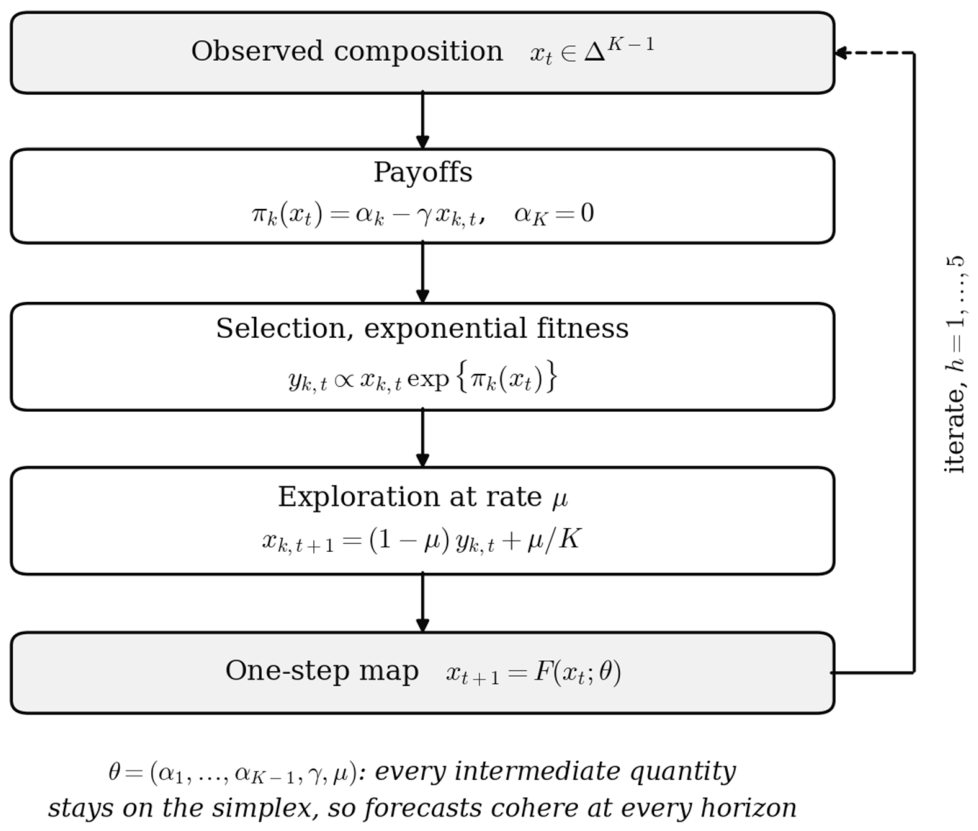Figure 1 sets out one application of the map in schematic form, from the observed composition through payoffs, selection and exploration to the next composition, together with the recursion that produces multi-step forecasts. Every intermediate quantity is a composition, so the forecasts cohere at every horizon without renormalisation.

The same map is easier to compare with the benchmarks in log-ratio coordinates. With $\mu =0$, taking the log-ratio of any part to the reference part on both sides of Equation (1) gives

$$\mathrm{l}\mathrm{n}{\displaystyle \frac{{\widehat{x}}_{k,t+1\mid t}}{{\widehat{x}}_{K,t+1\mid t}}}=\mathrm{l}\mathrm{n}{\displaystyle \frac{x_{k,t}}{x_{K,t}}}+{\alpha }_k-\gamma \left(x_{k,t}-x_{K,t}\right), k=1,\dots ,K-1.$$

(2)

Equation (2) says that the structural model is a random walk with drift in additive log-ratio coordinates whose drift is state-dependent: the constant part ${\alpha }_k$ is the drift of the classical benchmark, the term $-\gamma \left(x_{k,t}-x_{K,t}\right)$ is the frequency-dependent correction that the economics adds, and the mutation term of Equation (1) is a shrinkage of the whole vector toward the barycentre. The random walk with drift is therefore the special case $\gamma =0$, $\mu =0$, and the no-change forecast is the special case $\alpha =0$, $\gamma =0$, $\mu =0$. This nesting is what makes the results of Section 4 interpretable: the evolutionary restriction can only beat these two benchmarks if the curvature $\gamma$ and the smoothing $\mu$ are worth their estimation cost on the data at hand.

The parameters are estimated by conditional least squares in the geometry of the simplex. Writing $d_A\left(u,v\right)=\parallel \mathrm{c}\mathrm{l}\mathrm{r}\left(u\right)-\mathrm{c}\mathrm{l}\mathrm{r}\left(v\right){\parallel }_2$ for the Aitchison distance, the Euclidean distance between centred log-ratio images, the estimator at origin $t_0$ is

$$\widehat{\theta }=\mathrm{a}\mathrm{r}\mathrm{g}\underset{\theta }{\mathrm{m}\mathrm{i}\mathrm{n}}\hspace{0.25em}\sum _{i\in \mathcal{S}}\hspace{0.25em}\sum _{t<t_0}{d}_A{\left(x_{i,t+1},\hspace{0.17em}F\left(x_{i,t};\theta \right)\right)}^2,$$

(3)

where $\mathcal{S}$ is the set of units whose training data enter the objective, and it is through $\mathcal{S}$ that the sharing regime of Section 3.3 enters. The mutation rate is estimated on the logistic scale $\tilde{\mu }=\mathrm{l}\mathrm{n}\left(\mu /\left(1-\mu \right)\right)$ so that the parameter vector is unconstrained, and the optimiser, the starting values and the treatment of zero parts are described in Appendix A.3. Multi-step forecasts are produced by iterating the estimated map from the last observed composition, which yields a coherent path on the simplex at every horizon.

3.2. The Benchmarks in the Same Notation

Every benchmark has the same structure as Equation (1): a one-step map, iterated $h$ times, applied to the composition or to its log-ratio image. Writing $z_t=\mathrm{a}\mathrm{l}\mathrm{r}\left(x_t\right)$ for the additive log-ratio coordinates, $z_k=\mathrm{l}\mathrm{n}\left(x_k/x_K\right)$, the classical benchmarks forecast

$${\widehat{x}}_{t+h\mid t}={\mathrm{a}\mathrm{l}\mathrm{r}}^{-1}\left(G^h\left(z_t;\varphi \right)\right),$$

(4)

where in Equation (4), $G$ is the benchmark’s one-step map in log-ratio coordinates and $\varphi$ its parameter vector, and the inverse transform returns the forecast to the simplex, so that every forecast in the paper, structural or statistical, lies on the simplex by construction.

Table 1. Forecast functions, parameter vectors and free parameter counts by model and composition size. $z=\mathrm{a}\mathrm{l}\mathrm{r}\left(x\right)$ has $m=K-1$ coordinates; every map is iterated $h$ times and, where it operates on $z$, mapped back to the simplex by the inverse transform. VAR counts refer to the conditional mean. The two machine-learning benchmarks are non-parametric maps whose hyperparameters are listed in place of a parameter vector.

Model	One-Step Map	Parameters	K = 3	K = 4
No change	$z^{\prime }=z$	none	0	0
Random walk with drift	$z^{\prime }=z+\delta$	$\delta$	2	3
ARIMA, per coordinate	${z_k}^{\prime }$ = ARIMA(p, d, q) in $z_k$	order-dependent	varies	varies
Exponential smoothing, per coordinate	${z_k}^{\prime }$ = ETS with optional damped trend	order-dependent	varies	varies
VAR, lag order by AIC	$z^{\prime }=c+A_1 z+\dots +A_p z_{\left\{-p+1\right\}}$	c, A_1, …, A_p	6 (p = 1)	12 (p = 1)
Dynamic Dirichlet	$x^{\prime } ~$ Dirichlet $(\phi m(x\left)\right),$ $m\left(x\right)$ = C(exp $\left(\rho clr\right(x) + c))$	$c, \rho , \phi$	4	5
Replicator–mutator, Equation (1)	$x^{\prime }=F(x; \theta )$	$\alpha , \gamma , \mu$	4	5
Support vector regression, pooled	$z^{\prime }$ = SVR(z), radial basis kernel	$\left(C, \epsilon \right)\in \left\{1, 10\right\}\times \left\{0.05, 0.1\right\}$	tuned	tuned
Perceptron, pooled	$z^{\prime }$ = MLP(z), one hidden layer	(width, penalty) $\in \{4, 8\}$ $\times \{0.001, 0.1\}$	tuned	tuned
Equal-weight combination	clr average of five classical benchmarks and the pooled structural map	none	0	0

lists the one-step map and the parameter vector of each competitor and counts the free parameters at $K=3$ and $K=4$. The no-change benchmark repeats the last observed composition. The random walk with drift extrapolates the average log-ratio change over the training window. Univariate ARIMA and exponential smoothing models are fitted per coordinate with orders and trend components selected by corrected Akaike information [19]. A vector autoregression is fitted to the full log-ratio vector with lag order chosen by Akaike information. The dynamic Dirichlet comparator is a non-evolutionary transition model specified directly on the simplex, in the tradition of Grunwald, Raftery and Guttorp [20] and of the Dirichlet autoregressive models developed from it [21]: the next composition is Dirichlet distributed about a mean that follows a first-order recursion linear in the Aitchison geometry, with $K-1$ location parameters, a scalar persistence parameter and a precision, hence exactly $K+1$ free parameters, so that the comparison between the two dynamic families is not confounded with a difference in parameter counts; its estimation is described in Appendix A.4. Two pooled machine-learning benchmarks, a support vector regression with a radial basis kernel [22] and a single-hidden-layer perceptron [23], are fitted coordinate-wise to the pooled one-step log-ratio transitions of all countries in the training window and iterated exactly like the structural map, with their hyperparameters selected by walk-forward validation inside the training window; the equal-weight combination averages the five classical benchmarks and the pooled structural model in centred log-ratio coordinates. Appendix A.4 gives the implementation details, the fallback rules and the invariance of each benchmark to the choice of log-ratio reference.

The parameter counts explain why the restriction is worth testing. At $K=3$ the structural model has four parameters against six for the conditional mean of a first-order vector autoregression; at $K=4$ it has five against twelve, because the autoregressive parameterisation is quadratic in the number of coordinates while the structural one is linear in the number of parts. On a panel of $N$ units, the totals are $4N$ under country-specific estimation, 4 under full pooling and $4N+4$ under the shrunk regime at $K=3$, which is the arithmetic behind the sharing margin.

3.3. Parameter Sharing and Walk-Forward Selection

Let $\theta$ collect the parameters of Equation (1) in the unconstrained parameterisation. For a panel of units $i=1,\dots ,N$ three regimes are considered. Under the country-specific regime, ${\widehat{\theta }}_i$ is estimated on unit $i$’s training window alone, so that $\mathcal{S}=\left\{i\right\}$ in Equation (3). Under the pooled regime, a single ${\widehat{\theta }}_{\mathrm{p}\mathrm{o}\mathrm{o}\mathrm{l}}$ is estimated on all units’ training data jointly, $\mathcal{S}=\{1,\dots ,N\}$. Under the shrunk regime, the forecast for unit $i$ uses the convex combination

$${\theta }_i\left(\lambda \right)=\lambda \hspace{0.17em}{\widehat{\theta }}_i+\left(1-\lambda \right)\hspace{0.17em}{\widehat{\theta }}_{\mathrm{p}\mathrm{o}\mathrm{o}\mathrm{l}}, \lambda \in \{0,0.5,1\},$$

(5)

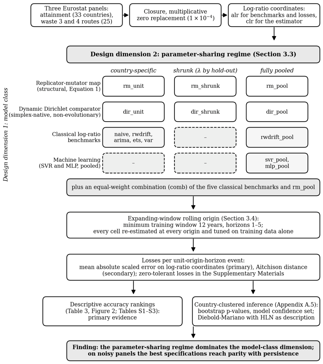
with $\lambda$ chosen for each unit and each origin by walk-forward validation; the training window is split into an estimation segment and a validation segment at its end, and both endpoints are estimated on the estimation segment; the candidate weights are scored on the validation segment, and the winner is re-estimated on the full training window before forecasting. The evaluation sample is never touched. Because the combination is taken in the unconstrained parameterisation, the implied mutation rate remains in the unit interval by construction. The words are used precisely below: the pooling regime is the design margin with three settings; parameter sharing covers the two settings that estimate anything in common; full pooling is the fully pooled endpoint alone. The dynamic Dirichlet comparator is estimated under the same three regimes with the same walk-forward selection, and the drift benchmark is estimated with country-specific and with pooled drift, the latter being the grand mean of one-step log-ratio changes across all countries in the training window, so that at least one purely statistical benchmark also varies its sharing regime. The two machine-learning benchmarks exist only in the pooled regime, for the reason given in Appendix A.4.

3.4. Data and Evaluation Protocol

Three panels are constructed from Eurostat online datasets, restricted to the longest run of consecutive annual observations from 2000 onward with at least eighteen years, and with the European Union and euro area aggregates removed so that every unit is a country. The attainment panel uses population by educational attainment level for ages 25 to 64, both sexes, in per cent (Eurostat online data code edat_lfse_03), partitioned into ISCED 2011 levels 0 to 2, 3 to 4, and 5 to 8; the three parts are an exact partition. The waste panels use municipal waste by treatment operation in thousands of tonnes (Eurostat online data code env_wasmun). The three-route version partitions treated municipal waste into recycling, including composting and digestion, incineration, including energy recovery, and landfill and other disposal, which together account for 99.6% of reported treated municipal waste on average and are reclosed to sum to one within every country-year; the four-route version splits recycling into material recycling and composting with digestion, giving a four-part composition on the same countries and years and allowing the parameter-count advantage of Table 1 to be exercised.

Table 2. Panel descriptives. Zero cells are parts reported as zero and subject to multiplicative replacement.

Panel	Parts	Countries	Years	Observations	Zero Cells	Origins	Target Years
Attainment	3	33	2000–2025	834	0 (0.0%)	438	2012–2025
Waste, 3 routes	3	25	2000–2024	609	111 (6.1%)	309	2012–2024
Waste, 4 routes	4	25	2000–2024	609	163 (6.7%)	309	2012–2024

gives the descriptives. The contrast between the panels is deliberate: attainment compositions are strongly and monotonically trending across Europe over this period, as the low-attainment share falls and the tertiary share rises, whereas municipal waste routes are noisier, subject to reporting revisions, and contain genuine structural zeros for countries that operate no incineration capacity. Zero parts are replaced multiplicatively before any log-ratio operation, with the replaced mass set to ${10}^{-4}$ in proportion units, identically for every model.

The evaluation is an expanding-window rolling origin. For each unit, every model is re-estimated at every origin using only data up to that origin, starting from a training window of twelve observations, and forecasts are produced for horizons one through five, truncated at the end of the sample. This applies to the structural model in full: the shrinkage weight, the pooled parameter vector and the unit-specific parameter vector are all recomputed at every origin from training data alone, as are the hyperparameters of the machine-learning benchmarks. Two losses are computed. The primary loss is the mean absolute scaled error of Hyndman and Koehler [24], computed on log-ratio coordinates, averaged over coordinates, and scaled by the in-sample mean absolute one-step no-change error of the corresponding training window, which makes it comparable across panels of different volatility; the secondary loss is the Aitchison distance between realised and predicted composition. Pairwise comparisons use the Diebold-Mariano statistic [25] with the small-sample correction of Harvey, Leybourne and Newbold [26] as descriptive evidence; every inferential statement rests on a bootstrap that resamples whole countries with replacement, which is the relevant clustering for a panel of national statistics, and on the model confidence set of Hansen, Lunde and Nason [27] computed at the 10% level by resampling complete country loss histories. With 25 to 33 country clusters, these p-values are approximations, so the substantive conclusions rest on the descriptive rankings and borderline test outcomes are treated with caution. Appendix A.5 gives the details, and Appendix A.6 tests the whole apparatus on simulated data of known provenance before it is applied to the real panels.

4. Results

4.1. One Table: The Sharing Margin Against the Model-Class Margin

Table 3. Mean absolute scaled error averaged over horizons one to five, all models and panels. rm and dir denote the replicator–mutator model of Equation (1) and the dynamic Dirichlet comparator; unit, pool and shrunk denote the country-specific, fully pooled and shrunk regimes of Section 3.3; rwdrift_pool is the drift benchmark with pooled drift, svr_pool and mlp_pool the pooled machine-learning benchmarks and comb the equal-weight combination. On the attainment panel, a dagger marks the nine models that the country-clustered model confidence set retains at every horizon. The sharing gain is the reduction from the country-specific regime to the better of the two sharing regimes; the model-class gap is the distance between the best structural specification and the best non-structural model on that panel.

Model	Attainment	Waste, 3 Routes	Waste, 4 Routes
rm_unit	1.564	3.196	2.796
rm_pool	1.129 †	2.992	2.503
rm_shrunk	1.167 †	2.706	2.242
dir_unit	1.455	2.530	2.368
dir_pool	1.119 †	2.769	2.537
dir_shrunk	1.139 †	2.393	2.198
Random walk with drift	1.115 †	2.780	2.363
rwdrift_pool	1.134 †	3.251	2.603
No change (naive)	2.140	2.417	2.011
ARIMA	1.151 †	2.898	2.506
Exponential smoothing	1.451	2.581	2.182
VAR	1.634	5.283	3.171
svr_pool	1.325 †	3.176	2.279
mlp_pool	1.456	3.001	2.430
comb	1.153 †	2.767	2.080
Sharing gain, replicator–mutator	27.8%	15.3%	19.8%
Sharing gain, dynamic Dirichlet	23.1%	5.4%	7.2%
Model-class gap	1.3%	13.1%	11.5%

contains the whole result. It reports the mean absolute scaled error averaged over horizons one to five for every model on every panel, with the two dynamic families arranged by sharing regime, and it closes with the two margins the paper is built to compare: the reduction in error from moving a family from country-specific estimation to its best sharing regime, and the gap between the best structural specification and the best non-structural model. 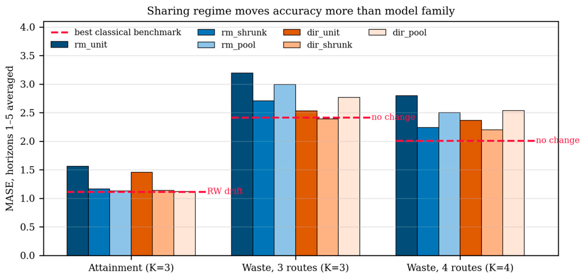Figure 2 draws the two dynamic families from the same table. Horizon-by-horizon tables, the win-rate analysis, the estimated parameters and the robustness checks under the Aitchison distance, the opposite log-ratio reference and alternative zero replacements are in the Supplementary Materials; none of them changes the ordering read here.

Three facts are visible at once. First, on every panel and in both dynamic families the country-specific regime is the worst specification of its family, and the gain from moving to the best sharing regime is large: 27.8% for the structural model on attainment, 15.3% and 19.8% on the waste panels, and 23.1%, 5.4% and 7.2% for the Dirichlet comparator. Second, the gap between the best structural specification and the best non-structural model is 1.3% on attainment and 13.1% and 11.5% on the waste panels, so on attainment the sharing decision is worth more than twenty times the structural-versus-statistical decision, and on the waste panels the two are of comparable magnitude, with the sharing margin the larger on both. In no case is the model class the dominant consideration. Third, the best sharing regime is not the same everywhere: on attainment it is full pooling, on both waste panels it is the validation-selected shrunk specification, and full pooling there is worse than shrinkage for the structural family and worse than country-specific estimation for the Dirichlet family and for the drift benchmark. The robust finding is therefore that an appropriately selected parameter-sharing regime improves accuracy, not that full pooling is uniformly beneficial; the title’s pooling is shorthand for this parameter-sharing margin.

The statistical support is as follows. On the attainment panel, the country-clustered model confidence set contains the same nine models at every horizon: the drift benchmark, the pooled drift benchmark, ARIMA, the equal-weight combination, the pooled support vector regression and the pooled and shrunk specifications of both dynamic families; in contrast, the no-change forecast, exponential smoothing, the VAR, the perceptron and both country-specific dynamic specifications are excluded throughout. Against the random walk with drift, the corrected Diebold-Mariano statistics for the shrunk structural model range from $-1.45$ to $-0.87$ across horizons, with country-clustered bootstrap p-values between 0.168 and 0.478. The structural model is therefore statistically indistinguishable from the best available forecast on this panel, without being better than it. On the waste panels, the no-change benchmark is never eliminated: it is alone in the set at horizon one on the three-route panel, the shrunk Dirichlet comparator enters from horizon two on the three-route panel and from horizon three on the four-route panel, and the sets widen with the horizon to as many as eleven of the fifteen models at horizon five, which is what resampling twenty-five country clusters can be expected to resolve. On the three-route panel, the shrunk Dirichlet comparator finishes marginally ahead of the no-change benchmark under the primary loss, 2.393 against 2.417, but the ordering reverses under the Aitchison distance, and country-clustered tests cannot distinguish the two, so the accurate statement is parity between persistence and the best simplex-native specification rather than dominance in either direction. Against the no-change benchmark, the structural model is significantly worse at the shortest horizons on both waste panels and insignificantly worse thereafter.

4.2. Economic Reading of the Ordering

Each row of Table 3 has an economic explanation, and the explanations are the same ones that motivated the restriction in Section 2.

The attainment panel is a diffusion process of the Griliches and Fisher-Pry kind: the low-attainment share falls, and the tertiary share rises monotonically in every country, and in log-ratio coordinates the paths are close to straight lines. On such data the random walk with drift, which extrapolates the average log-ratio change, is nearly the right model, and Equation (2) explains why the pooled structural model ties it rather than beats it. The structural map is the drift benchmark plus a frequency-dependent correction $-\gamma \left(x_k-x_K\right)$ plus a shrinkage toward the barycentre; when the log-ratio paths are already straight, the correction has little to add, and the two additional parameters are paid for in estimation variance. The pooled structural model at 1.129 and the pooled drift benchmark at 1.134 sit within half a per cent of each other, as the nesting predicts. The estimated congestion parameter nevertheless carries the economics of Section 2.2: its full-sample median on the attainment panel is $-0.074$; it is negative for 23 of 33 countries; and for eleven of the 33 countries the estimated map admits more than one numerically located rest point, so that the same dynamics imply different long-run attainment compositions from different starting points. That is the increasing-returns story of directed technical change and peer effects, read off a forecasting model estimated for a different purpose, and the stability analysis of Appendix A.2 confirms that negative $\gamma$ is exactly the condition under which the interior rest point of the map becomes unstable, and the attractors move toward the faces of the simplex. The reading is conjectural in one respect: nothing in the estimation ties $\gamma$ to auxiliary country-level information such as returns to education or intergenerational mobility, and testing it against such data is a study of its own.

The waste panels are congestion processes with noise. The estimated congestion parameter is positive, with medians of 0.109 on the three-route panel and 0.244 on the four-route panel, so that treatment routes crowd as capacity constraints and rising marginal disposal costs would imply, and the interior rest point of the map is locally stable for every positive estimate, as Appendix A.2 shows. But the year-to-year movement of the route mix around that rest point is dominated by reporting revisions and by structural zeros, and on such data the no-change forecast, which is the special case of Equation (2) with no drift and no curvature, is the hardest model to beat: every dynamic model, structural or statistical, estimates a direction of movement from twelve to twenty-five noisy observations and pays for it when the direction does not materialise. The Supplementary Materials make the mechanism explicit. On the 6.1% and 8.7% of forecast events whose realised composition contains a replaced zero, persistence of the replaced value is almost exactly right and every interior-valued dynamic model pays a large log-ratio penalty; on the zero-free majority of events the ranking inverts and the shrunk Dirichlet comparator is ahead of the no-change benchmark on both panels. The no-change benchmark’s lead on the waste panels is thus earned almost entirely on structural zeros, and the interesting forecasting problem on these panels is the zero-free interior, where the best simplex-native dynamic model is already ahead.

The sharing margin has the oldest explanation in forecasting: the bias-variance trade-off, with an economic gloss. At twelve to twenty-five annual observations per country, the sampling variance of four or five country-specific parameters swamps whatever heterogeneity bias pooling introduces, and the prior of Section 2.3, that the technology of adjustment is common across countries drawing on one regulatory and statistical space while the intercepts are not, is what the shrunk regime implements when it selects between the endpoints. That the Dirichlet family reproduces the sign of the effect, at a materially smaller size on the waste panels, shows that the margin belongs to the data environment rather than to the evolutionary restriction: it measures the value of information sharing in short panels, not a property of replicator dynamics. That full pooling hurts the Dirichlet model and the drift benchmark on the waste panels, and that the walk-forward selection chooses full pooling on roughly half of the unit-origins and no pooling on roughly a third, shows that the degree of sharing is a tuning decision that the data must be allowed to make, which is the subject of Section 6.

Two further results belong in the coherent set because they bound it. The machine-learning benchmarks land mid-field on every panel, ahead of country-specific structural estimation on attainment but behind the frontier of pooled specifications, and near the bottom on the three-route waste panel: the pooled sample of several hundred transitions is large enough for them to exploit but not large enough to reward flexibility over a four-parameter map. And the mutation rate is not a behavioural constant. Appendix A.3 shows that multiplicative observation noise on the simplex induces an inward drift with the same signature as mutation, so that the least-squares criterion loads measurement error onto $\widehat{\mu }$, and the Supplementary Materials report that imposing $\mu =0$ improves accuracy in every one of the nine panel-by-regime cells, by 0.9% to 17.2%, without changing any ordering. The estimated exploration rate should be read as a smoothing device selected on training data, which is the reading Section 6 builds on.

5. Discussion

5.1. The Result in the Forecasting Literature

The forecasting literature predicted the shape of this result before the data were seen, and the value of the exercise is in having measured it on compositional panels under a controlled design. Three of its strands are directly involved. The first is the long insistence, from the competitions of Makridakis and co-authors [28,29,30] to the survey of Petropoulos and co-authors [31], that simple methods are hard to beat and that claims of accuracy must be established with proper protocols. That an economic restriction ties the drift benchmark to trending data and loses to persistence on noisy data is neither surprising nor discreditable in that light; it is the expected outcome of testing a restriction out of sample rather than in sample.

The second strand is cross-learning and panel forecasting. The M4 and M5 competitions established that methods fitting one model to many series outperform series-by-series estimation; Montero-Manso and Hyndman [32] supply the formal argument for why global models can dominate local ones even on heterogeneous collections; Semenoglou and co-authors [33] document the accuracy of cross-learning methods; and Salinas and co-authors [34] give a prominent neural implementation. The panel-econometrics side of the same argument is older. Garcia-Ferrer, Highfield, Palm and Zellner [17] and Zellner and Hong [18] showed in the 1980s that shrinking country-specific coefficients toward a pooled mean improves international growth forecasts, and that estimator is the linear ancestor of Equation (5); Hoogstrate, Palm and Pfann [35] established that pooled estimates dominate in mean squared forecast error precisely when the time dimension is short relative to parameter heterogeneity; Baltagi [36] surveys the accumulated evidence that pooled and shrinkage estimators outforecast their heterogeneous counterparts in short panels; Liu, Moon and Schorfheide [37] give the modern empirical-Bayes treatment; and Pesaran, Pick and Timmermann [38] show that the advantage of pooling grows with estimation uncertainty and falls with heterogeneity, and that combinations of individual and pooled forecasts are the most reliable choice across configurations. The sharing result of Table 3 is the same economics in a nonlinear, simplex-valued setting with a handful of parameters, and the simulation grid of Appendix A.6 reproduces the ordering these papers predict: under the model’s own data-generating process, the best sharing regime beats country-specific estimation in every cell with homogeneous units, by 1.9% to 10.6%, while any appreciable heterogeneity hands the race to country-specific estimation at every sample length and noise level considered. The empirical dominance of sharing on the real panels is therefore not a small-sample artefact within the structural world; it indicates that the variance reduction obtained under misspecification and measurement noise outweighs a degree of parameter heterogeneity that would be decisive if the model were literally true.

The third strand is forecast combination. Timmermann [39] catalogues when combination pays and why equal weights are hard to beat; Claeskens, Magnus, Vasnev and Wang [40] show that estimating combination weights destroys the very optimality that motivates them; and Wang, Hyndman, Li and Kang [41] review the field. The Supplementary Materials report that win rates and mean losses diverge on the attainment and three-route panels, with the model that wins the most individual forecast events not being the model with the lowest mean loss, which is the classic signature of loss profiles that differ across event types and the classic argument for combination over selection. The equal-weight combination tested here finishes 3.4% behind the best single model on attainment and on the four-route waste panel and 15.6% behind on the three-route panel, and beats it nowhere, which is what the combination puzzle predicts when one of the components is already close to optimal; weighted or selective combination is a hypothesis for future work rather than a recommendation of this paper. The nonlinear and machine-learning strand completes the picture: Teräsvirta [42] concludes that carefully specified nonlinear models beat linear ones only intermittently, Zhang, Patuwo and Hu [23] catalogued how sensitive neural forecasters are to specification and sample length, Hewamalage, Bergmeir and Bandara [43] document how much data recurrent architectures need before they become competitive, and Zeng and co-authors [44] show a one-layer linear model matching transformer-based forecasters on standard benchmarks, while Medeiros, Vasconcelos, Veiga and Zilberman [45] and Smyl [46] show machine-learning methods winning when data are pooled on a scale annual official statistics cannot supply. The mid-field placement of the two pooled machine-learning benchmarks in Table 3 is consistent with every strand of that evidence.

5.2. The Result in Economics

For the evolutionary economics the restriction came from, the result has three implications. The first concerns practice. An author who estimates an evolutionary model country by country and reports in-sample fit is making the choice that the evidence identifies as most damaging to out-of-sample performance on panels like these, and the fix, a validation-selected sharing regime, improved accuracy on every panel. The compositional data analysis tradition [2,47,48,49] and its recent likelihood-based branch [21,50,51,52] supply the geometry and the coherence, but they are agnostic about where the dynamics come from; the evolutionary tradition [9,10,11] supplies the dynamics but has almost never asked them to forecast. The design used here joins the two under the protocol of the forecasting literature, and the joint answer is that the economics survives as interpretation while the accuracy comes from sharing.

The second implication concerns interpretation. The sign of the congestion parameter sorted the panels exactly as the theoretical examples of Section 2.2 predicted: negative under the increasing returns of directed technical change and peer effects in attainment, and positive under the congestion of capacity-constrained disposal routes; moreover, the multistability of the attainment map is the lock-in of Arthur [15] appearing in a forecasting model. These are the conclusions the applied literature draws from in-sample fits, and the point of the present design is that they survive a protocol that the fits themselves would not have survived: the estimates are interpretable even though the restriction that produced them does not forecast better than its own special cases. The mutation rate is the exception, and Appendix A.3 shows why: exploration and measurement noise leave the same second-order signature on the simplex, so no prior, penalty or profile likelihood restores a behavioural reading of $\widehat{\mu }$ from public aggregates; only auxiliary knowledge of the measurement process, such as design-based sampling variances of the underlying surveys, could do so.

The third implication concerns what a negative result is for. Once the structural and statistical families are known to sit within about one per cent of each other on the attainment panel, the fifteen to twenty-eight per cent attached to the parameter-sharing decision stops being one result among many and becomes the only design choice in this environment with a first-order effect on out-of-sample accuracy, and it is the choice the applied literature currently makes by default and in the more expensive direction. A study that had found the restriction to pay would have left that margin undiscovered.

5.3. Scope and Limitations

The scope of the claim should be stated exactly, because the evidence supporting it is narrow in five respects. The panels are three, drawn from two subject domains and a single statistical producer; the frequency is annual; the country series are short, with a minimum training window of twelve observations and at most twenty-six at the final origin; the cross-section is twenty-five to thirty-three national units; and the comparator set is the classical log-ratio family, one simplex-native likelihood model and two pooled machine-learning benchmarks, with recurrent and transformer-based forecasters excluded for the scale reasons given in Appendix A.4. What the evidence supports is accordingly a conditional statement: in short annual compositional panels of official statistics, where per-unit estimation uncertainty is large relative to genuine cross-unit parameter heterogeneity, the choice of parameter-sharing regime moves out-of-sample accuracy more than the choice between an evolutionary restriction and a generic log-ratio benchmark. Appendix A.6 marks the boundary of that condition from the other side, since moderate or strong heterogeneity reverses the ranking in every cell of the grid, and Pesaran, Pick and Timmermann [38] give the analytical reason. Whether the ordering survives at higher frequency, on longer histories, in other domains or against cross-learning competitors at scale is an open empirical question, and the title of the paper names the regime studied here rather than a law of compositional forecasting.

Five limitations qualify the findings. First, and most seriously, the mutation parameter is not separately identified from observation noise, for the reason given above; for the forecasting purpose of the paper, the defect is contained, because $\mu$ enters the evaluation only as a smoothing device selected on training data and judged out of sample, and the Supplementary Materials verify that imposing $\mu =0$ leaves every conclusion intact. Second, the waste panels contain 6.1% and 6.7% zero cells, which the multiplicative replacement handles identically for all models but which inflates every log-ratio loss and is part of why no dynamic model succeeds there; the zero-tolerant losses reported in the Supplementary Materials, computed on the raw share scale, show the pooled Dirichlet model overtaking persistence under the Jensen-Shannon divergence on both waste panels, so the ranking of persistence against the best simplex-native model is the one conclusion that does not survive every treatment, and it is reported as parity for that reason. Third, the payoff specification is deliberately minimal; a richer structure with strategy-specific congestion or covariates entering the intercepts would add parameters and, on the evidence of Table 3, would need to be pooled to be useful, and covariates would change the exercise from unconditional to conditional forecasting. Fourth, for the minority of units with strongly negative congestion estimates, forecasts are launched inside basins of attraction whose boundaries move with the parameter estimates, so estimation error can relocate the configuration toward which the iterated map travels; the short horizons used here and the damping factor $1-\mu$ keep the risk contained, but longer-horizon use in the increasing-returns regime should be preceded by the stability audit that Appendix A.2 makes mechanical. Fifth, the shrinkage of Equation (5) is discrete selection over a coarse grid with one weight for the whole parameter vector, not hierarchical partial pooling; a proper hierarchical estimator that shrinks each parameter separately is the first extension the next section motivates.

6. Tuning the Parameters by Walk-Forward Optimisation

The evidence of Section 4 identifies two parameters of the structural forecast function as tuning devices rather than structural constants: the shrinkage weight $\lambda$, whose selected value varies across units and origins, and the mutation rate $\mu$, whose freely estimated value contributes variance without predictive content. A third dial, the degree of sharing applied to different blocks of the parameter vector, is implicit in the prior of Section 2.3. All three are natural objects for walk-forward optimisation, the sequential procedure in which tuning parameters are chosen on a validation segment inside the training window, applied to the next out-of-sample period, and re-chosen as the window advances. The design of this paper already uses that procedure for $\lambda$ and for the hyperparameters of the machine-learning benchmarks; what follows generalises it to the structural model and states what the evidence says about each dial.

The procedure is as follows. At origin $t_0$ the training window of unit $i$ is split into an estimation segment and a validation segment consisting of its last $q$ years; the rule used for the machine-learning benchmarks here, a quarter of the window with a minimum of two years, is a reasonable default. On the estimation segment, the country-specific and pooled parameter vectors are estimated by Equation (3) for every candidate value of the tuning vector $\left(\lambda ,\mu \right)$, with $\lambda$ on a grid in the unit interval and $\mu$ either fixed at zero, fixed at a grid value, or freely estimated. Each candidate is scored on the validation segment by the multi-horizon loss actually used for evaluation, the scaled error averaged over the horizons the forecaster will be asked to produce, so that the selection criterion and the evaluation criterion coincide. The winning candidate is then re-estimated on the full training window and used to forecast horizons one to five from $t_0$; the window is advanced by one year, and the procedure repeats, so that the tuning vector is re-optimised at every origin and no forecast uses information beyond its origin. Because the search is nested inside the rolling origin, the resulting accuracy is an honest out-of-sample measure of the tuned forecaster, and because the same nesting is applied to every competitor, the comparison remains fair.

The evidence bounds what each dial can deliver. For the shrinkage weight, the walk-forward selection over the coarse grid $\{0,0.5,1\}$ chose full pooling on 49.1%, 49.5% and 50.5% of the unit-origins on the three panels, no pooling on 27.4%, 32.4% and 31.7%, and the intermediate weight on the remaining 23.5%, 18.1% and 17.8%. Refining the grid to eleven points in the unit interval moved accuracy by a few percent and in both directions, from 2.706 to 2.621 and from 2.242 to 2.216 on the waste panels but from 1.167 to 1.206 on attainment, and it redistributed weight away from the corners without eliminating them, the endpoints being chosen in 58% to 66% of unit-origins against 77% to 82% under the coarse grid; the selected weight also switched between adjacent origins more often under the fine grid, 36% to 44% of the time against 17% to 23%. The lesson for a walk-forward implementation is that the candidate set should be kept coarse when the validation segment is short, because a rich menu adds selection noise that a validation window of a few years cannot resolve, and that the corner frequencies describe what such a window can resolve rather than a natural division of countries into homogeneous and heterogeneous types.

For the mutation rate, the evidence is one-sided. Fixing $\mu =0$ improved accuracy in all nine panel-by-regime cells, by 0.9% to 17.2%, with the largest gains for the country-specific regime on the waste panels, exactly where the recovery experiment of Appendix A.6 predicts the estimated rate to be least reliable; imposing the cross-country median instead helped the country-specific regime but hurt the pooled one, whose own estimated smoothing level is smaller. A walk-forward search should therefore always include $\mu =0$ in the candidate set and treat the freely estimated rate as one candidate among others, and it should expect the selection to favour zero or a small fixed value on panels this short. The third dial, parameter-specific sharing, is not implemented here and is the natural next step: the prior of Section 2.3 suggests pooling the adjustment parameters $\gamma$ and $\mu$ while allowing the intercepts to vary, which a walk-forward search can test by letting the shrinkage weight differ between the two blocks, and a hierarchical random-coefficient formulation of the map with second-level variances estimated across countries would replace the grid search with a proper estimator. Two cautions apply to any such extension. The validation segment must be taken from the end of the training window, never from its interior, because the losses that matter are those of forecasts launched from the most recent state; and an expanding window is preferable to a fixed-length rolling window on panels of twelve to twenty-six observations, because the variance cost of discarding early observations dominates the bias cost of structural change at these lengths, though a fixed-length window becomes the right choice once the history is long enough for the trade-off to reverse.

7. Conclusions

We specified a discrete-time replicator–mutator map as a forecast function for compositional time series, showed that it nests the random walk with drift and the no-change forecast as special cases, estimated it under three parameter-sharing regimes, and evaluated it, together with a non-evolutionary dynamic Dirichlet comparator under the same regimes, against classical log-ratio benchmarks, a pooled drift benchmark, two pooled machine-learning benchmarks and an equal-weight combination on three Eurostat panels with a rolling-origin design, scale-free losses, country-clustered tests of equal predictive ability and model confidence sets.

The evolutionary restriction does not pay for itself in accuracy. It matches the best benchmark on educational attainment, where it enters the model confidence set at every horizon, and it loses to a no-change forecast on municipal waste routes, as does every other dynamic model except the shrunk dynamic Dirichlet comparator, which reaches parity there. What does pay is parameter sharing: moving from country-specific estimation to the best sharing regime, full pooling on attainment and validation-selected shrinkage on the waste panels, reduces scaled error by 15.3% to 27.8% across the three panels, an effect larger than the one separating the best structural model from the best benchmark, and it reappears with the same sign in a non-evolutionary family. The estimated congestion parameters nevertheless sort the panels as the economics predicts, with increasing returns in attainment and congestion in waste routes, so the restriction earns its keep as interpretation rather than as accuracy.

For applied researchers using evolutionary dynamics on panels of official statistics, the operative message is that the parameter-sharing decision deserves at least as much attention as the specification of payoffs, that the shrinkage weight and the mutation rate should be selected by walk-forward optimisation inside the training window rather than fitted in sample, and that out-of-sample evaluation should be the standard rather than the exception. Two boundaries travel with that message. The comparison is against classical log-ratio benchmarks, one simplex-native likelihood model and two pooled machine-learning benchmarks rather than against cross-learning methods at the scale of long and wide corpora, and the panels are short, annual and drawn from a single statistical producer; a simulation grid shows the ordering reversing once cross-country parameter heterogeneity is appreciable. Within those boundaries the ordering is clear, tested and reproducible; outside them it is a hypothesis. The contribution is accordingly not the failure of one restriction but the relocation of the design margin: in this data environment the question worth asking of a compositional forecasting model is not which dynamics it imposes, but how much of its parameter vector is estimated in common across units.