Multiscale Visibility Forecasting over Complex Terrain Using High-Temporal-Resolution WRF Fields and a Physics-Informed Spatial Prior

Highlights

What are the main findings?

• A coarse-to-fine WRF-ConvLSTM framework enables 1-km hourly visibility forecasting up to 12 h over complex terrain.
• A CVIS-derived physics-informed spatial prior improves fine-scale reconstruction despite its limited standalone forecasting performance.

What are the implications of the main findings?

• High-temporal-resolution WRF fields and physics-informed spatial priors provide complementary dynamic and spatial information.
• The framework provides a practical approach to continuous visibility forecasting in data-sparse mountainous regions.

Abstract

Atmospheric visibility is an important meteorological variable affecting transportation, tourism, and agricultural production. Guizhou Province, located in the eastern Yunnan-Guizhou Plateau, has complex terrain and high humidity and is prone to fog-related low-visibility events. To meet the need for refined forecasts over complex terrain while reducing the cost of direct high-resolution forecasting over large areas, this study integrates high-temporal-resolution WRF (Weather Research and Forecasting) forecasts with deep learning to develop a multiscale model that combines coarse-scale spatiotemporal prediction with fine-scale spatial reconstruction. It provides hourly, spatially continuous visibility forecasts across Guizhou. The following results are established: (1) Multiscale WRF-ConvLSTM (MS-WRF-ConvLSTM) improves low-visibility forecasting compared with other models. For the next 12 h, R ranges from 0.59 to 0.73 and RMSE from 0.81 to 1.01 km, while categorical scores indicate reliable event identification and stable performance across lead times. (2) By integrating multiscale information and learning regional spatial relationships, the model improves spatial continuity and local detail, making it suitable for refined forecasting over complex terrain. (3) Ablation experiments confirm the contributions of the multiscale structure, high-temporal-resolution data, and CVIS spatial constraint. Although CVIS has limited direct predictive accuracy, its spatial prior improves fine-scale reconstruction and balances accuracy with spatial detail. (4) SHAP analysis identifies historical visibility, elevation, slope, wind direction, dew-point temperature, air temperature, and specific humidity as important predictors. Learned spatial relationships among cities further improve regional visibility prediction.

1. Introduction

Atmospheric visibility is generally defined as the maximum horizontal distance at which the outline of a target can be discerned by the human eye under specific meteorological conditions [1]. It is influenced by aerosol composition, meteorological conditions, precipitation, and boundary-layer structure, and can decrease markedly during heavy rainfall, dust events, fog, and haze. Fog is a common weather phenomenon in Guizhou, and the resulting reduction in visibility affects socioeconomic activities and residents’ daily lives [2]. Persistent low-visibility events can cause widespread flight delays [3], temporary highway closures, direct economic losses, and safety risks. Therefore, accurate visibility forecasting is essential for improving meteorological services and transportation safety.

Current visibility forecasting methods mainly include physically based numerical models, empirical statistical methods, and rapidly developing machine-learning approaches. Numerical models simulate fog formation and evolution by resolving atmospheric physical and dynamical processes and provide key variables such as the extinction coefficient, relative humidity, droplet number concentration, and liquid/ice water content [4]. These variables are commonly used in visibility parameterization schemes [5]. Kunkel proposed the K84 scheme, which relates liquid/ice water content to visibility [6] and improves the accuracy of visibility estimation. The National Oceanic and Atmospheric Administration (NOAA) developed the FSL scheme [7], which has been widely applied in operational aviation meteorology. This scheme estimates visibility using near-surface air temperature, dew-point temperature, relative humidity, and empirical coefficients. Empirical statistical methods use regression and correlation analyses of observations to quantify relationships between visibility and relevant factors and subsequently develop regional empirical models. Previous studies have successfully identified the effects of multiple factors on visibility using statistical analyses [8]. However, these methods have limited applicability under complex weather conditions.

With the rapid development of machine learning and deep learning, data-driven models have become an important means of capturing nonlinear relationships between visibility and multiple influencing factors. Peláez-Rodríguez et al. [9] developed a deep-learning ensemble model for low-visibility events associated with radiation and orographic fog. Their model outperformed individual deep-learning models, conventional machine-learning methods, and meteorological benchmarks. Zhu et al. [10] used hourly observations from Urumqi International Airport to establish relationships between meteorological variables and visibility, thereby developing a visibility regression model for operational airport guidance. Lu et al. [11] proposed an intelligent offshore visibility forecasting method combining a temporal convolutional network (TCN) with transfer learning to address limited observations and complex weather conditions. The method achieved satisfactory performance in the Qiongzhou Strait.

Nevertheless, existing visibility forecasting studies still have several limitations. Many studies [12] focus on single-station forecasts and primarily capture temporal variations, with limited ability to predict spatially continuous regional visibility fields. In complex terrain, low-visibility events exhibit strong locality and spatial heterogeneity because their formation and evolution are jointly affected by terrain, moisture transport, and local circulation [13]. High-spatial-resolution meteorological fields are therefore required. However, directly applying such data to large-area forecasting substantially increases computational costs and model training time. Achieving continuous spatial prediction while retaining local details and controlling computational costs remains a major challenge.

Guizhou Province is located in the eastern Yunnan-Guizhou Plateau and is characterized by extensive mountainous and valley terrain. Complex moisture transport, orographic lifting, and local circulation contribute to frequent low-visibility events. Compared with those over plains, these events show stronger locality and spatial heterogeneity, and conventional meteorological stations cannot fully represent regional visibility variations [3]. High cloud cover also limits the application of satellite remote-sensing data to visibility forecasting [14,15]. Consequently, high-spatiotemporal-resolution visibility forecasting is particularly important for Guizhou.

This study focuses on low-visibility forecasting over the complex terrain of Guizhou and proposes a coarse-to-fine multiscale visibility forecasting framework that integrates the Weather Research and Forecasting (WRF) model with deep learning. Coarse-scale spatiotemporal prediction reduces the computational burden of direct high-resolution forecasting over large areas, while spatial prior information derived from multisource data is incorporated into fine-scale reconstruction to generate spatially continuous visibility forecasts for the next 12 h. The proposed model is compared with conventional deep-learning forecasting models to evaluate differences in predictive performance. Typical low-visibility events and SHapley Additive exPlanations (SHAP) are further used to identify the key factors affecting the formation and evolution of low visibility in Guizhou. By integrating high-spatiotemporal-resolution numerical simulations with multisource data, this study provides methodological and data support for refined visibility forecasting over complex terrain.

2. Data and Methods

2.1. Data and Study Area

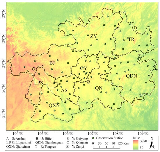
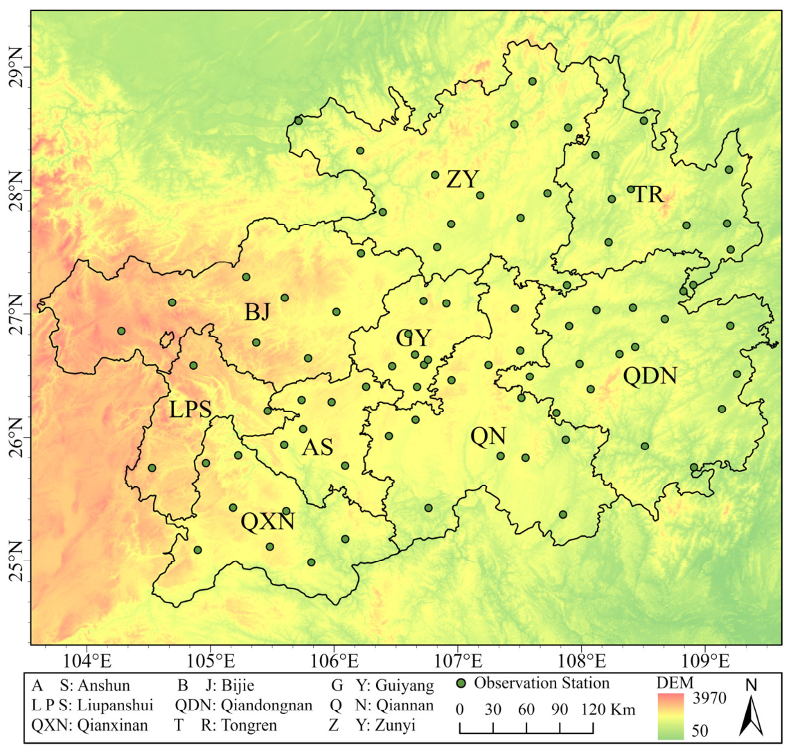
This study covers the entire Guizhou Province, China. Owing to the combined effects of complex terrain, large elevation variations, and regional weather systems, low-visibility events associated with frontal, orographic, and radiation fog occur frequently in the study area, significantly affecting transportation, socioeconomic activities, and public travel safety. For low-visibility forecasting, a multisource meteorological and geographical dataset covering 2022–2024 was collected and constructed. The dataset mainly comprises Final Operational Global Analysis (FNL) fields, Global Forecast System (GFS) fields, land-surface data, and hourly observations from surface meteorological stations across Guizhou. The NCEP FNL data were primarily used to provide initial and boundary conditions for historical case simulations (https://gdex.ucar.edu/datasets/d083002/, (accessed on 1 August 2026)), whereas the GFS data were used to provide meteorological boundary conditions for operational forecasts and predictions at future lead times (https://gdex.ucar.edu/datasets/d084001/, (accessed on 1 August 2026)). The land-surface data include land cover, elevation, and slope. Land-cover data were obtained from the MCD12Q1 product, elevation data were obtained from the Shuttle Radar Topography Mission (SRTM) dataset [16], and slope was derived from the elevation data. Hourly observations from surface automatic weather stations included air temperature, relative humidity, wind speed, and minimum visibility. A total of 84 stations were distributed across all cities and districts in Guizhou Province, with a relatively high station density in the central and eastern regions and a lower density in the high-elevation mountainous areas of the west. This distribution was closely associated with topographic variability and local conditions for station installation. Overall, the station network provided adequate coverage to characterize spatial variability across different terrain settings. The spatial distribution of the stations is shown in Figure 1.

Figure 1. Spatial distribution of observation stations.

Because the datasets differ in spatial resolution and grid alignment, their direct use as model inputs may introduce spatial mismatch errors. To ensure spatial consistency, all meteorological fields and land-surface datasets were uniformly preprocessed and resampled to a spatial resolution of 1 km, thereby producing a gridded dataset consistent with the model input requirements.

2.2. Research Method

2.2.1. Multiscale Joint Visibility Forecasting Framework

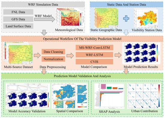
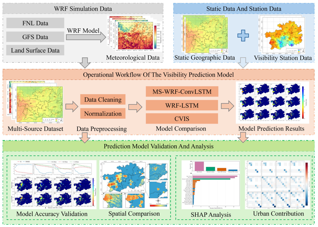
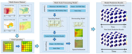
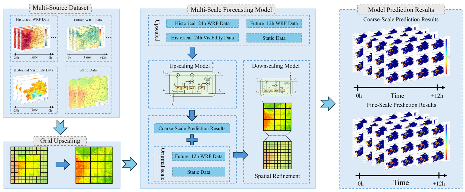
Owing to its complex terrain and humid climate, Guizhou Province experiences persistently high cloud cover, which limits the continuity and availability of satellite remote-sensing data for monitoring and early warning of low-visibility events [3]. In addition, automatic visibility observation stations are relatively sparse across the region, making it difficult to establish a refined prediction network covering the entire province [15]. To address these limitations, a multisource dataset for 12-h visibility forecasting over Guizhou was constructed by integrating WRF forecast fields, station-based visibility observations, static geographical data, and CVIS-derived visibility fields. Two deep-learning models were subsequently developed. The first is the proposed Multiscale WRF-ConvLSTM (MS-WRF-ConvLSTM) model, which adopts a two-stage structure consisting of coarse-scale spatiotemporal prediction and fine-scale spatial reconstruction. WRF meteorological fields, static geographical information, and CVIS-derived visibility fields are incorporated into the fine-scale reconstruction stage, enabling the model to account for the temporal evolution, spatial structure, and physical constraints of visibility. The second is a conventional LSTM model used as a baseline to quantify the improvement provided by the multiscale spatiotemporal fusion approach. Finally, the resulting 12-h visibility forecasts over Guizhou were evaluated in terms of predictive accuracy, spatial differences, SHAP-based feature contributions, and intercity contributions, as illustrated in Figure 2.

Figure 2. Flowchart of the Visibility Forecasting Process.

2.2.2. WRF Model Simulation Configuration

The model data used in this study were generated using the WRF model at a temporal resolution of 10 min. FNL analyses were used to drive WRF simulations for the preceding 24 h, while GFS forecasts provided the input boundary conditions for simulations covering the subsequent 12 h. The simulations covered Guizhou Province from 1 January 2022 to 31 December 2024. The physical parameterization schemes followed those adopted by Zhu et al. [17], who investigated the effects of improved WRF static data on quasi-stationary frontal fog simulations over complex terrain. Their configuration was designed to improve the simulation of frontal fog, making it well aligned with the visibility prediction objectives of the present study. Its applicability to Guizhou Province has also been explored in previous research. This configuration was therefore adopted to generate high-resolution meteorological fields tailored to complex terrain and fog processes, providing more reliable air temperature, humidity, and wind fields for subsequent machine learning model training. The specific physical parameterization schemes are listed in Table 1.

Table 1. WRF model configuration and parameter settings.

Model Information	Setting
Model version	WRF V4.3.3
d01, d02, d03 Number of grids	(83, 82), (127, 118), (235, 205)
d01, d02, d03 spatial resolution	27 km, 9 km, and 3 km
Physical parameterization scheme	YSU, Grell-3, RRTM, Dudhia, Noah, Purdue Lin
Meteorological fields	FNL reanalysis data GFS forecast data

2.2.3. CVIS Visibility Algorithm

To provide spatial-distribution constraints for the MS-WRF-ConvLSTM model, prior visibility fields were calculated using the CVIS algorithm and WRF output variables. The CVIS algorithm was proposed by Bang et al. [18] by combining the FSL and SW99 algorithms, with the minimum of their respective visibility estimates selected as the final result. A previous study [19] compared the performance of several conventional numerical-model-based visibility algorithms over China and found that CVIS achieved markedly higher accuracy than the other algorithms. The CVIS algorithm is formulated as follows:

$$FSL =6000\times {\displaystyle \frac{T2-TD2}{{RH2}^{1.75}}}$$

(1)

$$SW99={\displaystyle \frac{-\mathrm{l}\mathrm{n}\left(0.02\right)}{144.7{CW}^{0.88}+1.1{RW}^{0.75}+163.9{CI}^{1.00}+10.4{SN}^{0.78}}}$$

(2)

$$CVIS=\min \left(FSL,SW99\right)$$

(3)

Here, T2 and TD2 denote the 2-m air temperature and 2-m dew-point temperature, respectively, while RH2 represents the 2-m relative humidity. The variables CW, RW, CI, and SN represent the water contents of cloud water, rainwater, cloud ice, and snow, respectively.

2.2.4. Development of the Coarse-to-Fine Joint Forecasting Model

Because low-visibility events accounted for only a small proportion of the samples, a piecewise scaling approach was adopted to improve the model’s ability to learn from these events. Visibility values within 0–1 km were mapped to the normalized interval of 0–0.7, whereas values within 1–30 km were compressed into the interval of 0.7–1.0. Model predictions were subsequently transformed back to the original visibility range of 0–30 km using the inverse mapping. By allocating 70% of the normalized range to visibility values within 0–1 km, this transformation amplified numerical differences among low-visibility samples in the loss function, thereby increasing their relative weight during training and enhancing the model’s sensitivity to changes in low visibility. The scaling and inverse mapping equations are given below:

$${VIS}_{scale} = \{\begin{array}{l}0.7 \times VIS, 0\le VIS\le 1\\ 0.7 + {\displaystyle \frac{0.3(VIS - 1)}{30 - 1}}, 1<VIS<30\end{array}$$

(4)

$$VIS=\{\begin{array}{l}{\displaystyle \frac{{VIS}_{scale}}{0.7}}, 0 \le {VIS}_{scale} \le 0.7\\ 1+{\displaystyle \frac{30-1}{0.3}}\left({VIS}_{scale}-0.7\right), 0.7<{ VIS}_{scale} \le 1\end{array}$$

(5)

where $VIS\left(Km\right)$ denotes the actual visibility, and ${VIS}_{scale}$ denotes the scaled visibility.

The deep learning models used in this study are described below.

• ConvLSTM forecasting model

ConvLSTM is a spatiotemporal sequence modeling method that integrates convolutional neural networks (CNNs) with long short-term memory (LSTM) networks. Convolutional operations are used to capture local spatial correlations, whereas the recurrent structure, memory cells, and gating mechanisms of LSTM are employed to represent temporal evolution. ConvLSTM therefore combines spatial feature extraction with temporal dependency modeling. Compared with conventional CNN or LSTM models, ConvLSTM can simultaneously capture long-term temporal dependencies and spatial structures, making it suitable for forecasting meteorological variables with pronounced spatiotemporal continuity.

Given the large spatial extent of Guizhou Province, direct long-sequence, large-area, high-resolution spatiotemporal forecasting would require substantial computation and GPU memory and may reduce training stability. A joint forecasting scheme consisting of coarse-scale prediction and fine-scale reconstruction was therefore developed. First, the multisource meteorological data were spatially aggregated, and multiple spatial statistics were calculated within each window, reducing the spatial dimensions of the raster data over Guizhou to one-tenth of their original size. The coarse-scale model then used the aggregated WRF data from the preceding 24 h, interpolated station observations from the preceding 24 h, WRF forecasts at future target times, and static geographical variables to predict the minimum, maximum, and mean visibility over the coarse-resolution grid for the subsequent 12 h. The fine-scale model subsequently used the coarse-scale forecasts as constraints and combined them with WRF forecasts and static land-surface data at the original spatial resolution for each future target time. The spatial distribution of CVIS-derived visibility was further used to reconstruct the coarse-scale forecasts and generate fine-scale visibility predictions. This two-stage framework reduces the computational complexity of direct high-resolution forecasting over a large area while retaining fine-scale spatial structures and improving the spatial detail of regional visibility forecasts. The proposed multiscale joint forecasting model is referred to as the Multiscale WRF-ConvLSTM (MS-WRF-ConvLSTM) model, and its workflow is shown in Figure 3.

Figure 3. Schematic diagram of the multiscale integrated forecasting framework of the MS-WRF-ConvLSTM model.

2.

Baseline LSTM Forecasting Model

To provide a comparison with the joint spatiotemporal modeling approach of MS-WRF-ConvLSTM, a visibility forecasting model based on multisource data and a conventional LSTM architecture, referred to as WRF-LSTM, was developed. WRF-LSTM does not explicitly represent the spatial structure among adjacent grid cells or perform multiscale spatial reconstruction. Instead, it extracts pixel values corresponding to station locations from the multisource dataset to construct a station-based sample dataset covering Guizhou Province. The model uses WRF data and station observations from the preceding 24 h, WRF forecasts for the subsequent 12 h, and static geographical variables as inputs to predict visibility at the corresponding grid cells over the next 12 h, thereby producing pixel-scale visibility forecasts.

2.2.5. Evaluation Metrics

A holdout validation strategy was adopted to evaluate the accuracy of the WRF-LSTM and MS-WRF-ConvLSTM models. Data from 2022 to 2023 were used for model training, data from January to September 2024 were used as the test set, and data from October to December 2024 were used as the event-based validation set. The performance of the WRF meteorological model was evaluated hourly against observations from surface meteorological stations.

The accuracy of the WRF simulations was assessed using the root-mean-square error (RMSE), mean bias (MB), and correlation coefficient (R). For the visibility forecasting models, R and RMSE were used to evaluate continuous visibility predictions, whereas the threat score (TS), recall (also referred to as the hit rate), and bias score (BS) were used to evaluate categorical visibility forecasts. The corresponding equations are given below.

$$RMSE=\sqrt{{\displaystyle \frac{{\displaystyle {\sum }_{i=1}^n}{(x_i-y_i)}^2}{n}}}$$

(6)

$$MB={\displaystyle \frac{{\displaystyle {\sum }_{i=1}^n}(x_i-y_i)}{n}}$$

(7)

$$R={\displaystyle \frac{{\displaystyle {\sum }_{i=1}^n}(x_i-\overline{x})(y_i-\overline{y})}{\sqrt{{\displaystyle {\sum }_{i=1}^n}{(x_i-\overline{x})}^2}\sqrt{{\displaystyle {\sum }_{i=1}^n}{(y_i-\overline{y})}^2}}}$$

(8)

$$TS={\displaystyle \frac{TP}{TP+FP+FN}}$$

(9)

$$Recall={\displaystyle \frac{TP}{TP+FN}}$$

(10)

$$BS={\displaystyle \frac{TP+FP}{TP+FN}}$$

(11)

Here, $x_i$ denotes the observed value at a meteorological station, and $x_i$ represents the mean of the station observations. Similarly, $y_i$ denotes the model-predicted value, and $\overline{y}$ represents the mean of the model predictions. TP denotes the number of cases in which both the model prediction and the observation indicate a positive event; FN denotes the number of cases in which the model prediction is negative while the observation is positive; and FP denotes the number of cases in which the model prediction is positive while the observation is negative.

3. Results and Analysis

3.1. Evaluation of Meteorological Model Performance

Meteorological station observations were used to evaluate the performance of the daily 12-h WRF forecasts during 2022–2024 for T2, 10-m wind speed (WS10), 10-m wind direction (WD10), RH2, and hourly precipitation (PRE) (Table 2), thereby assessing the reliability and applicability of the model data. For T2, the RMSE of the WRF simulations was 2.30 K, which was comparable to values reported in previous studies [20,21,22]. The mean bias (MB) was −0.21 K, meeting the recommended criterion of ±0.5 K [23], and the correlation coefficient was relatively high (R = 0.83), indicating that WRF effectively reproduced regional temperature variations. For WS10, the RMSE was 2.0 m/s, meeting the recommended criterion of RMSE ≤ 2.0 m/s [23], while the correlation coefficient was 0.49, supporting the reliability of the wind-speed simulations. For WD10, the RMSE was below 60°, the MB was within ±10°, and the correlation coefficient was 0.50. These results met the wind direction performance criteria adopted in previous research for regions with complex terrain [24]. Although no explicit performance benchmark is currently available for RH2, its RMSE, MB, and R values were comparable to those reported in previous studies [25,26], indicating that WRF adequately reproduced the variations in relative humidity. For hourly precipitation, the RMSE and MB were 0.21 and 0.03, respectively, indicating relatively small errors and limited systematic bias. Simulated and observed precipitation were positively correlated, although the correlation was weak (R = 0.32). This is attributable to the localized nature and spatial heterogeneity of precipitation [27,28].

Table 2. Performance evaluation of the WRF model.

Feature Factor	RMSE	MB	R
T2 (K)	2.30	−0.21	0.83
WS10 (m/s)	2.00	0.99	0.49
WD10 (degree)	59.93	5.19	0.50
RH2 (%)	14.26	−4.33	0.75
PRE (mm/h)	0.21	0.03	0.32

Overall, the WRF simulations showed good performance for air temperature, wind speed, wind direction, relative humidity, and hourly precipitation, adequately representing the meteorological characteristics of Guizhou and supporting their use in subsequent applications.

3.2. Correlation Analysis and Selection of Model Predictors

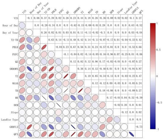
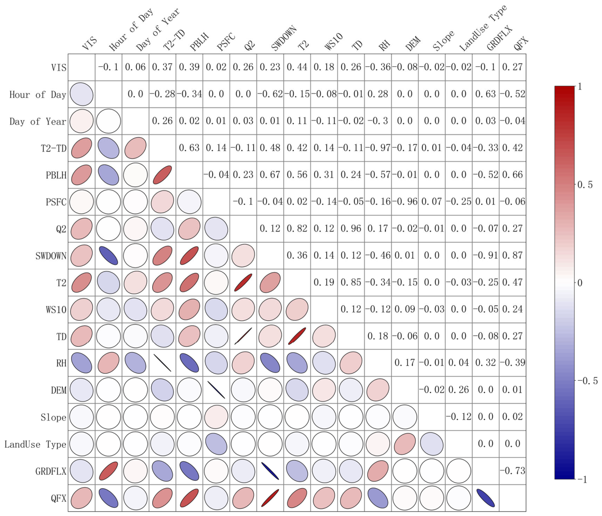
To examine the relationships between visibility and multiple WRF output variables, land-surface data, and temporal variables, Pearson’s correlation analysis was performed, and the results are shown in Figure 4. Day of year, dew-point depression, planetary boundary layer height, surface pressure, specific humidity, surface shortwave radiation flux, 2-m air temperature, 10-m wind speed, 2-m dew-point temperature, and water vapor flux were significantly positively correlated with target visibility (p < 0.001). In contrast, hour of day, 2-m relative humidity, elevation, ground heat flux, slope, and land use were significantly negatively correlated with visibility (p < 0.001). Among these variables, 2-m air temperature had the highest absolute correlation with visibility (r = 0.44), whereas slope and land use had the lowest absolute correlations (r = −0.01 and −0.04, respectively), indicating weak linear relationships.

Figure 4. Correlation heatmap of WRF-derived features. In an ellipse plot, a flatter ellipse indicates a stronger correlation, while a rounder one indicates a weaker correlation. Its color and orientation show whether the correlation is positive or negative.

Previous studies have reported positive relationships between visibility and variables such as 2-m air temperature, 2-m dew-point temperature, 10-m wind speed, and boundary layer height [29,30], consistent with the present results. Higher relative humidity promotes the hygroscopic growth of particles and the formation of fog droplets [31], thereby enhancing atmospheric extinction and reducing visibility. Elevation was also negatively correlated with visibility, indicating that high-elevation areas in Guizhou do not necessarily experience better visibility. This relationship may be associated with orographic lifting, moisture convergence, and cloud and fog activity over complex mountainous terrain. By contrast, the effects of slope and land-use type are spatially heterogeneous and nonlinear and should be considered together with terrain relief, temperature and humidity conditions, and local circulation [32]. Accordingly, their absolute Pearson’s correlation coefficients were below 0.1. Day of year and hour of day were included to represent the seasonal and diurnal variations in visibility. Although day of year was positively correlated with visibility and hour of day was negatively correlated, both variables are periodic. Their correlation coefficients therefore represent only the overall linear relationships within the samples and should not be interpreted as monotonic temporal increases or decreases in visibility.

Previous studies have shown that historical visibility observations can reflect preceding atmospheric conditions and the persistence of visibility evolution [33]; model inputs can therefore improve forecasting accuracy. Accordingly, station-based visibility observations over a preceding time window were introduced as an initial visibility predictor to enhance the model’s representation of temporal continuity and short-term variations. However, constraints related to station distribution and data availability limited the representation of different land-use types among the selected stations. The resulting lack of sample diversity may limit the broader applicability and generalization of the visibility forecasting model. Land-use data were therefore used solely to update the underlying surface characteristics in WRF and were not included as static predictors in the visibility forecasting model.

Based on the correlation analysis and considering both the relevance and physical interpretability of each variable, day of year, hour of day, T2, TD2, planetary boundary layer height (PBLH), surface pressure (PSFC), RH2, WD, WS, specific humidity (Q2), downward shortwave radiation flux at the surface (SWDOWN), elevation, slope, and historical visibility were ultimately selected as input features. These variables represent temporal variations, near-surface thermal conditions, atmospheric moisture, boundary layer structure, and terrain characteristics, thereby providing a relatively comprehensive description of the major processes affecting visibility and an effective basis for model development.

3.3. Forecast Performance and Spatial Adaptability of the Multiscale Model

3.3.1. Evaluation of Forecasting Model Performance

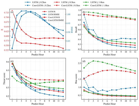
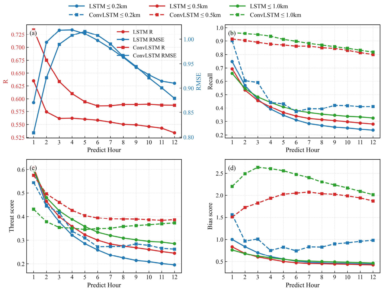
Selected high-visibility (VIS > 1 km) and low-visibility (VIS ≤ 1 km) events in 2024 were used for model validation. The forecasting capability of MS-WRF-ConvLSTM over the complex terrain of Guizhou was evaluated through comparison with WRF-LSTM. The validation results for high-visibility events are presented in Table 3, while those for low-visibility events and different visibility categories are shown in Figure 5. The key metrics are summarized in Table S1 in the Supplementary Materials.

Table 3. Comparison of forecasting accuracy for high-visibility events.

Predict Hour	MS-WRF-ConvLSTM					WRF-LSTM
	R	RMSE	TS	Recall	BS	R	RMSE	TS	Recall	BS
1	0.78	4.49	0.78	0.79	0.79	0.48	3.57	0.76	0.93	1.16
2	0.78	5.20	0.70	0.71	0.71	0.48	4.91	0.73	0.92	1.19
3	0.76	5.29	0.67	0.67	0.68	0.51	5.90	0.74	0.93	1.19
4	0.76	5.34	0.66	0.67	0.67	0.54	6.63	0.76	0.94	1.18
5	0.76	5.43	0.68	0.68	0.69	0.56	7.20	0.78	0.95	1.17
6	0.76	5.50	0.70	0.70	0.71	0.57	7.65	0.79	0.95	1.16
7	0.76	5.58	0.71	0.72	0.73	0.57	8.01	0.81	0.96	1.14
8	0.76	5.61	0.73	0.74	0.75	0.57	8.30	0.82	0.96	1.13
9	0.76	5.66	0.75	0.75	0.76	0.57	8.52	0.83	0.97	1.12
10	0.76	5.69	0.76	0.77	0.78	0.56	8.69	0.84	0.97	1.12
11	0.76	5.70	0.78	0.79	0.80	0.55	8.85	0.85	0.97	1.11
12	0.75	5.72	0.80	0.80	0.81	0.54	8.99	0.86	0.97	1.11

Figure 5. Verification of visibility-category forecasting performance. Continuous prediction accuracy, including (a) the R and RMSE metrics; (b) recall; (c) TS score; and (d) BS score.

For high-visibility events, MS-WRF-ConvLSTM showed good numerical fitting ability and stable performance across forecast lead times. Its R values ranged from 0.75 to 0.78, consistently exceeding the range of 0.48–0.57 obtained by WRF-LSTM. The RMSE ranged from 4.49 to 5.72 km and was lower than that of WRF-LSTM at all lead times except the first two forecast hours, indicating better representation of visibility variations and greater stability across lead times. In the categorical evaluation, MS-WRF-ConvLSTM achieved TSs of 0.70–0.80, recall values of 0.67–0.80, and BS values of 0.67–0.81. Although some low bias remained, the model maintained stable identification performance for high-visibility events.

The predictive performance for low-visibility events was further evaluated. WRF-LSTM achieved R values of 0.53–0.63 and RMSE values of 0.87–1.02 km, whereas MS-WRF-ConvLSTM achieved R values of 0.59–0.73 and RMSE values of 0.81–1.01 km. Overall, MS-WRF-ConvLSTM showed higher correlations and lower prediction errors, indicating that the combination of multiscale WRF features and the ConvLSTM architecture improves the representation of the spatiotemporal evolution of low-visibility events. The performance of both models decreased with increasing forecast lead time, consistent with the progressive accumulation of forecast errors in numerical weather prediction and deep-learning models [34].

Low-visibility events were further classified into three categories: VIS ≤ 200 m, VIS ≤ 500 m, and VIS ≤ 1000 m. MS-WRF-ConvLSTM maintained relatively stable identification performance across these categories. The hit rates for VIS ≤ 500 m and VIS ≤ 1000 m decreased from 0.91 to 0.80 and from 0.96 to 0.82, respectively, while that for VIS ≤ 200 m decreased from 0.90 to 0.40, indicating that the model retained some forecasting capability for severe low-visibility events at longer lead times. The threat scores (TSs) generally decreased with increasing forecast lead time. Nevertheless, MS-WRF-ConvLSTM maintained relatively high TS values for VIS ≤ 500 m and VIS ≤ 1000 m and showed reasonable stability for VIS ≤ 200 m except during the initial forecast period. The bias scores (BSs) further revealed systematic errors in the predicted frequencies of different low-visibility categories. WRF-LSTM generally produced BS values below 1 for all categories, indicating a tendency toward underforecasting. MS-WRF-ConvLSTM showed some overforecasting for VIS ≤ 500 m and VIS ≤ 1000 m, whereas its BS values for VIS ≤ 200 m were generally close to 1, indicating a relatively accurate representation of the frequency of severe low-visibility events. Overall, MS-WRF-ConvLSTM effectively represented the spatiotemporal variations of low-visibility events of different intensities over the complex terrain of Guizhou and maintained relatively stable performance across forecast lead times.

Furthermore, the model developed in this study achieved substantially higher forecast accuracy than that reported in previous research for Guizhou Province [3]. That study developed a U2-Net visibility forecasting model primarily using CMA-GD numerical forecasts and CLDAS gridded observations. However, in situ observations from multiple stations were not fully integrated into model training, which may have limited forecast accuracy. In comparison, the present model achieved better overall performance at identical or comparable visibility thresholds and forecast lead times. This improvement can be largely attributed to the joint use of high-resolution WRF meteorological predictors and observations from multiple stations, enabling the model to learn systematic discrepancies between numerical model outputs and surface observations and to better capture the combined effects of temperature, humidity, wind, and precipitation on visibility variations over the complex terrain of Guizhou Province.

3.3.2. Analysis of Regional Forecast Differences over Complex Terrain

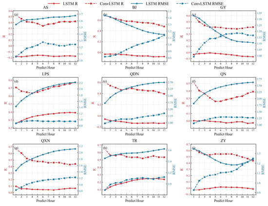
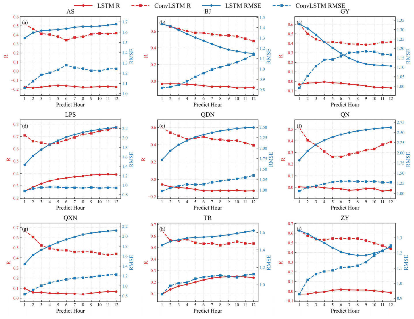
To examine regional differences in visibility prediction accuracy across the complex terrain of Guizhou Province in greater detail, model predictions were evaluated against station observations using the province’s nine prefecture-level administrative divisions as statistical units. Because the observation stations are distributed and managed according to administrative boundaries, this approach provides a reasonable number of samples within each unit and facilitates comparisons of WRF performance across different parts of the province. Guizhou is generally characterized by an elevation gradient descending from west to east, with a mosaic of plateaus, mountains, hills, and river valleys. Consequently, its prefecture-level divisions differ markedly in topography, elevation, underlying surface conditions, and local circulation. Although administrative boundaries do not strictly correspond to topographic or climatic zones, analyses at this administrative level can nevertheless capture, to some extent, the spatial heterogeneity of model errors over complex terrain.

The R and RMSE results (Figure 6) show that MS-WRF-ConvLSTM maintained relatively stable forecasting performance across all prefecture-level regions. In Liupanshui, where low-visibility events occur frequently, the model achieved R values of 0.68–0.75, indicating good agreement with observed visibility variations. This performance may be related to the greater number of low-visibility samples in this region, which provided sufficient information for model training [35]. In Anshun, Bijie, Guiyang, Qiandongnan, Qiannan, and Zunyi, where WRF-LSTM yielded negative R values, MS-WRF-ConvLSTM maintained favorable correlations and relatively low prediction errors. These regions feature complex terrain comprising mountains, hills, river valleys, and local basins. Topographic variations can locally modulate near-surface winds, moisture transport, cold-air pooling, and boundary-layer stability, resulting in pronounced spatial heterogeneity in visibility [36]. Limitations in WRF spatial resolution and boundary-layer parameterization prevent the full representation of small-scale terrain features and the associated local dynamical and thermodynamic processes [37]. Moreover, the conventional WRF-LSTM model primarily captures temporal dependencies and has a limited capacity to represent spatial relationships among stations, potentially reducing correlations in regions with strong spatial heterogeneity. By contrast, MS-WRF-ConvLSTM jointly extracts multiscale spatial features and temporal evolution patterns, thereby mitigating the effects of complex terrain and local biases in the input fields on visibility predictions.

Figure 6. Comparison of R and RMSE for the two models across the nine prefecture-level regions. Panels (a–i) correspond to different cities.

The categorical evaluation results (Supplementary Figures S1–S3) further demonstrate that MS-WRF-ConvLSTM maintained stable identification performance for low-visibility events across different regions and visibility categories. Although WRF-LSTM achieved higher recall in some regions, its relatively low TS values indicate that the higher hit rates were accompanied by more false alarms. In contrast, MS-WRF-ConvLSTM achieved a better balance among hits, misses, and false alarms. The BS results show that WRF-LSTM substantially overforecast VIS ≤ 200 m events in several regions, including Qiandongnan and Qiannan, whereas the BS values of MS-WRF-ConvLSTM were generally concentrated within 0.9–1.5, indicating closer agreement between the predicted and observed event frequencies. Considering R, RMSE, recall, TS, and BS together, MS-WRF-ConvLSTM exhibited stable and comprehensive forecasting performance across the prefecture-level regions of Guizhou, demonstrating its adaptability to local spatial differences in visibility over complex terrain.

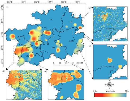
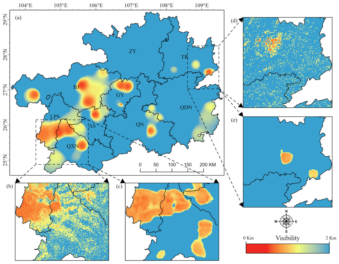
To further evaluate the model’s ability to represent local spatial features, a forecast at lead hour 5 was selected for spatial comparison (Figure 7). The WRF-LSTM prediction exhibited a pronounced scattered distribution and relatively weak spatial continuity. This is mainly because WRF-LSTM predicts individual-pixel time series and makes limited use of spatial relationships among neighboring pixels. In contrast, MS-WRF-ConvLSTM simultaneously extracts temporal evolution and spatial neighborhood features through the ConvLSTM architecture, producing a more spatially continuous forecast field that is more consistent with the station-interpolated visibility distribution. Prediction biases and limited spatial continuity in WRF-LSTM were particularly evident in cities such as Anshun and Bijie, which are characterized by complex terrain, sparse observation networks, and pronounced variability in local meteorological conditions. These deficiencies may be attributed to the limited ability of the WRF input data to fully represent the effects of complex terrain and underlying surface conditions on local visibility. Furthermore, conventional LSTM primarily captures temporal dependencies and has a limited capacity to represent spatial relationships among stations and spatial heterogeneity, resulting in poorer spatial prediction performance. These results indicate that MS-WRF-ConvLSTM can more effectively represent local differences and spatial variations in visibility over the complex terrain of Guizhou, demonstrating better spatial forecasting capability and regional adaptability.

Figure 7. Comparison of spatial details among different visibility forecasting models. (a) Station-interpolated visibility field at the selected forecast time. (b,d) Forecasts from the WRF-LSTM model. (c,e) Forecasts from the MS-WRF-ConvLSTM model.

3.4. Ablation Analysis of the Multiscale Model Architecture and CVIS Constraint

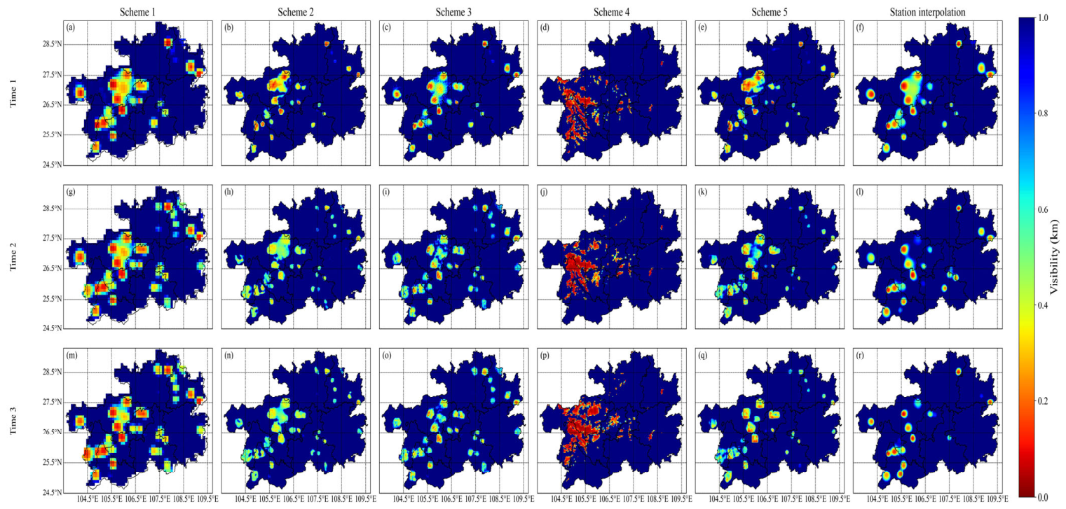
To evaluate the validity of the proposed multiscale visibility forecasting architecture, the effect of input temporal resolution and the contributions of individual model components were evaluated by comparing low-visibility (VIS ≤ 200 m) forecasts from different model schemes. The proposed model uses high-temporal-resolution WRF data and consists of coarse-scale and fine-scale forecasting components, which generate visibility fields at their respective spatial scales. The fine-scale model also incorporates the CVIS-derived visibility field as a spatial constraint to improve the representation of local low-visibility structures. Accordingly, the forecasting performance of the coarse-scale model, the fine-scale model with and without the CVIS spatial constraint, and the CVIS algorithm itself was compared to assess the effectiveness of the multiscale architecture and CVIS constraint. The evaluation results are presented in Table 4 and summarized in Table S1 in the Supplementary Materials. Schemes 1–4 use meteorological data at 10-min intervals, whereas Scheme 5 uses hourly meteorological data. Specifically, Scheme 1 represents the coarse-scale forecasting model; Scheme 2 represents the CVIS-constrained multiscale forecasting model; Scheme 3 represents the multiscale model without the CVIS constraint; Scheme 4 represents the visibility diagnosed directly using the CVIS algorithm; and Scheme 5 represents the CVIS-constrained multiscale model driven by hourly meteorological data. Notably, the CVIS algorithm in Scheme 4 estimates visibility from WRF outputs using empirical parameterizations developed in previous studies. Its applicability may be affected by the study period, regional climate, terrain, and errors in simulated hydrometeors [38], potentially resulting in biases in the diagnosed location, spatial extent, and intensity of fog.

Table 4. Accuracy comparison of numerical visibility forecast products.

Predict Hour	Scheme 1		Scheme 2		Scheme 3		Scheme 4		Scheme 5
	R	RMSE	R	RMSE	R	RMSE	R	RMSE	R	RMSE
1	0.25	0.12	0.32	0.12	0.26	0.14	0.16	0.45	0.26	0.16
2	0.21	0.16	0.30	0.17	0.24	0.17	0.20	0.45	0.21	0.21
3	0.17	0.18	0.25	0.19	0.18	0.20	0.15	0.45	0.17	0.25
4	0.16	0.20	0.25	0.21	0.19	0.22	0.14	0.46	0.17	0.27
5	0.15	0.22	0.23	0.21	0.17	0.23	0.09	0.49	0.17	0.29
6	0.16	0.22	0.22	0.22	0.17	0.24	0.13	0.47	0.18	0.30
7	0.17	0.23	0.21	0.22	0.17	0.26	0.06	0.49	0.19	0.31
8	0.18	0.23	0.21	0.23	0.18	0.26	0.16	0.48	0.19	0.32
9	0.19	0.24	0.21	0.23	0.19	0.27	0.09	0.48	0.20	0.33
10	0.19	0.25	0.22	0.24	0.19	0.28	0.08	0.49	0.21	0.34
11	0.21	0.27	0.23	0.25	0.21	0.30	0.05	0.50	0.22	0.35
12	0.23	0.29	0.24	0.25	0.23	0.32	0.00	0.51	0.23	0.36

The performance statistics indicate that Scheme 2 performed favorably in forecasting low visibility. Specifically, Scheme 1 yielded R values of 0.15–0.25 and RMSE values of 0.12–0.29, suggesting that the coarse-scale model captured some variability in low visibility, although forecast errors remained. Scheme 2 refined the coarse-scale forecasts using the CVIS outputs as a spatial constraint, achieving R values of 0.21–0.32 and RMSE values of 0.12–0.25. Scheme 3, which omitted the CVIS constraint from the fine-scale model, showed poorer overall performance than Scheme 2, with R values of 0.17–0.26 and RMSE values of 0.14–0.32. Scheme 5, in which the temporal resolution of the WRF input data was reduced to hourly intervals, also exhibited some deterioration in performance relative to Scheme 2, with R values of 0.17–0.26 and RMSE values of 0.16–0.36. Scheme 4 performed the worst, yielding R values of 0.00–0.20 and RMSE values of 0.45–0.51, indicating a limited ability to capture low-visibility variations and relatively large overall errors.

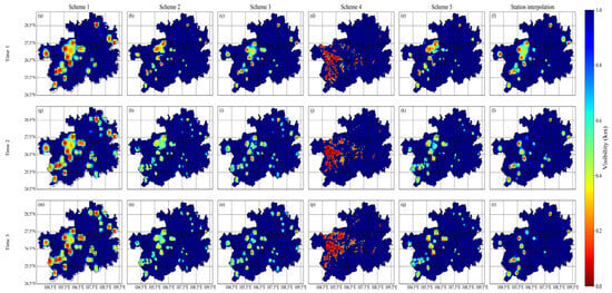
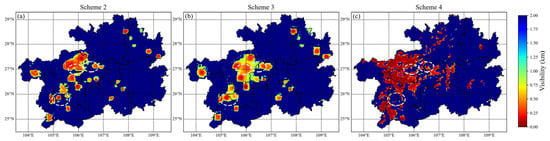
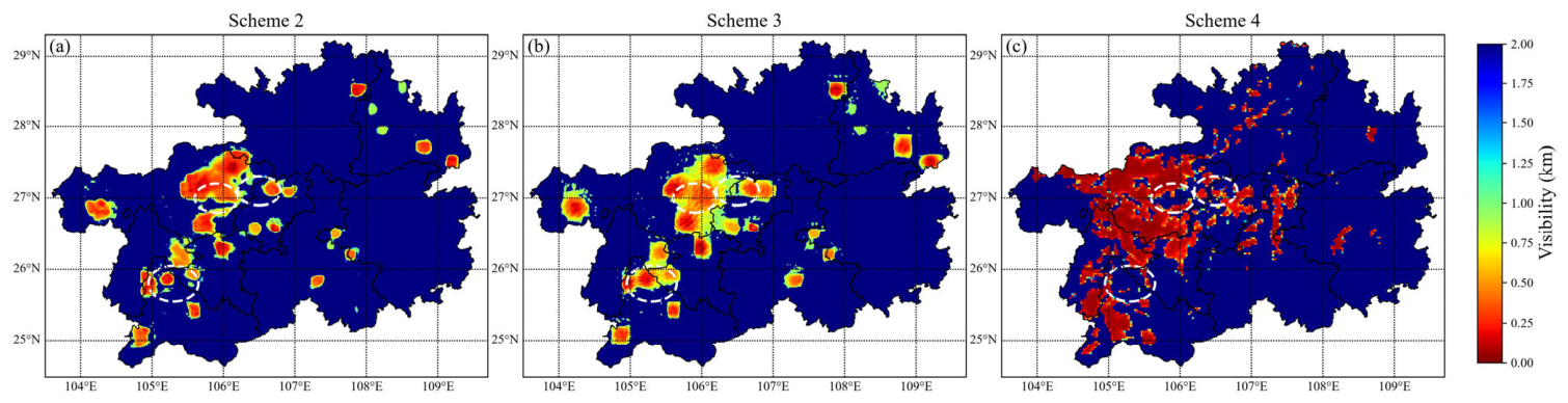
Interpolated station observations were further introduced as a spatial reference field to compare the visibility distributions predicted by the five schemes, as shown in Figure 8. The interpolated observations indicate that low-visibility areas were mainly concentrated in western Guizhou and localized parts of central Guizhou, with a distinct patchy distribution reflecting strong spatial heterogeneity over complex terrain. Except for Scheme 4, all schemes reproduced the main spatial distribution of low-visibility areas and showed good overall agreement with the station-interpolated field. Scheme 1, representing the coarse-scale forecast, captured the principal low-visibility areas. However, its relatively low input resolution produced an overly smooth forecast field and weakened the representation of local low-visibility centers and boundary variations. In contrast, Schemes 2, 3, and 5 used fine-scale forecasting structures and therefore represented spatial details more effectively. Among them, Scheme 2 showed the closest agreement with the station-interpolated field in terms of the locations, extents, and spatial patterns of low-visibility areas and effectively recovered local variations in the observed field. Further comparison in Figure 9 shows that Schemes 2 and 4 produced similar local low-visibility structures within the areas marked by white dashed circles and identified several fine-scale low-visibility centers, whereas Scheme 3 failed to recover these local spatial features effectively.

Figure 8. Spatial distributions produced by different schemes. Panels (a–r) compare the results of Schemes 1–5 with the station-interpolated fields at three different times, respectively.

Figure 9. Comparison of spatial details associated with the CVIS constraint. Panels (a–c) show the results of Schemes 2–4, respectively, and the white circles indicate the comparison areas.

Overall, Scheme 2 maintained relatively high numerical forecasting accuracy while providing more refined spatial reconstruction, achieving a better balance between prediction accuracy and the representation of spatial details.

3.5. Model Performance During Low-Visibility Events

To objectively evaluate the forecasting capability of MS-WRF-ConvLSTM during an actual low-visibility event, a typical event over Guizhou Province from 12:00 on 8 December to 03:00 on 10 December 2024 was selected for case validation. At the beginning of the event, low visibility mainly occurred in Liupanshui and eastern Bijie and gradually expanded eastward, reaching its first maximum spatial extent at 21:00 on 8 December. The affected area subsequently decreased. From 06:00 on 9 December, widespread low visibility redeveloped across the study area and continued to expand, reaching its maximum extent at approximately 15:00. The low-visibility area persisted until approximately 19:00 and then gradually weakened, becoming localized by 03:00 on 10 December.

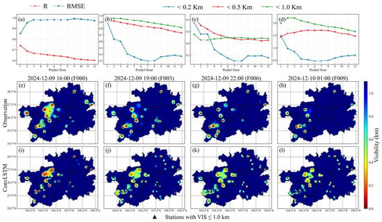
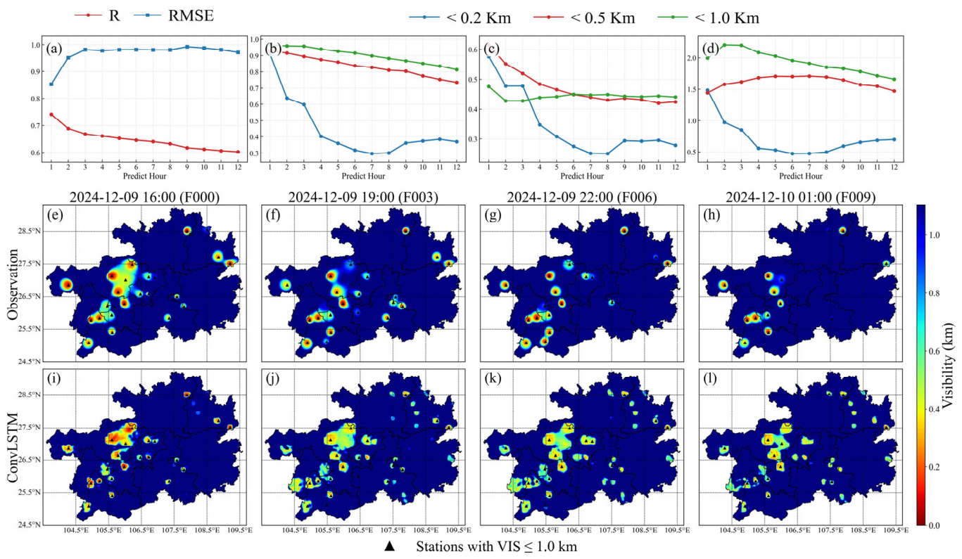
The forecasting performance of MS-WRF-ConvLSTM for this event is shown in Figure 10. Overall, the model maintained relatively stable forecasting performance. In terms of numerical accuracy (Figure 10a), R values mainly ranged from 0.60 to 0.74, while RMSE values ranged from 0.85 to 0.99 km. These results indicate that the model effectively represented temporal variations in near-surface visibility, although some magnitude errors remained. The categorical metrics (Figure 10b–d) show that the model maintained high and relatively stable identification performance for VIS ≤ 0.5 km and VIS ≤ 1.0 km, with recall and threat score decreasing only gradually as forecast lead time increased. For the extremely low-visibility category of VIS ≤ 0.2 km, recall and TS were relatively high during the first 3 h but decreased markedly at lead times of 4–12 h. This result indicates that the model effectively identified extremely low-visibility events at short lead times, but its ability to represent the persistence of extremely low values weakened with increasing lead time. The BS results further reveal differences in forecast bias among the visibility categories. Events with VIS ≤ 0.5 km and VIS ≤ 1.0 km were generally overforecast, whereas events with VIS ≤ 0.2 km gradually shifted toward underforecasting during the middle and later forecast periods.

Figure 10. Verification of the MS-WRF-ConvLSTM model for the low-visibility event. Panels (a–d) show the R and RMSE, recall, TS, and BS metrics, respectively. Panels (e–h) show the station-interpolated visibility fields at the corresponding times. Panels (i–l) show the spatial forecasts generated by the MS-WRF-ConvLSTM model initialized at 16:00 on 9 December 2024.

The observed spatial distributions (Figure 10e–l) show that low-visibility areas were mainly concentrated in western and west-central Guizhou and underwent pronounced spatial evolution at different forecast lead times. The model reproduced the primary locations of low-visibility areas and their temporal evolution, particularly over Liupanshui, Bijie, Guiyang, and surrounding areas, where the low-visibility centers and their outward expansion were reasonably represented. The model also captured the gradual improvement in visibility during the later stage of the event. The predicted low-visibility areas contracted over time, consistent with the observed evolution. However, the forecast fields exhibited some spatial smoothing compared with the observations. The intensity of extremely low visibility near several stations was underestimated, while the spatial extent of low visibility was overestimated in some peripheral areas.

The errors described above can be attributed to the natural conditions of the study region and the limited spatial resolution of the meteorological model. Western and west-central Guizhou exhibit substantial topographic relief, with mountains and valleys strongly modulating near-surface winds, moisture transport, and cold-air pooling. Under weak winds, high humidity, and stable boundary-layer conditions, valleys and low-lying areas are prone to moisture accumulation and near-surface temperature inversions [36], leading to localized patches of dense fog. However, the model’s limited spatial resolution prevents these small-scale terrain-induced dynamical and thermodynamic processes from being fully resolved [39]. Consequently, smoothing in the model outputs and subsequent spatial predictions can lead to overestimation of local visibility and underestimation of the severity of dense fog.

Supplementary Figures S4 and S5 further present continuous forecasts during the key stages of this event. Supplementary Figure S4 shows the rapid development and spatial expansion of low visibility, whereas Supplementary Figure S5 presents its maintenance and gradual dissipation. The model correctly reproduced the overall spatial evolution during both stages. The temporal evaluation metrics and spatial comparisons collectively demonstrate that MS-WRF-ConvLSTM effectively captured the formation, development, maintenance, and weakening of this low-visibility event, as well as the locations and evolution of the affected areas. These results indicate that the model is suitable for short-term low-visibility forecasting over complex terrain.

3.6. Analysis of Model Feature Importance and Spatial Associations

The SHapley Additive exPlanations (SHAP) method is based on game theory [40] and quantifies the marginal contribution of each input feature to model predictions, allowing its relative importance and direction of influence to be assessed. To evaluate the ability of MS-WRF-ConvLSTM to represent the factors affecting visibility over the complex terrain of Guizhou, SHAP was used for model interpretation. The contributions of historical visibility, WRF meteorological fields, and static variables were analyzed over the full sample, and a target-source administrative-region SHAP contribution matrix was constructed for a typical low-visibility event to examine spatial associations between regional input information and predictions for the target region. These associations should be interpreted as statistical relationships rather than evidence of physical transport processes.

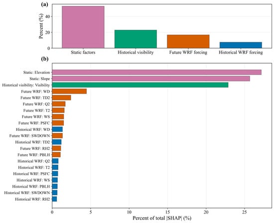
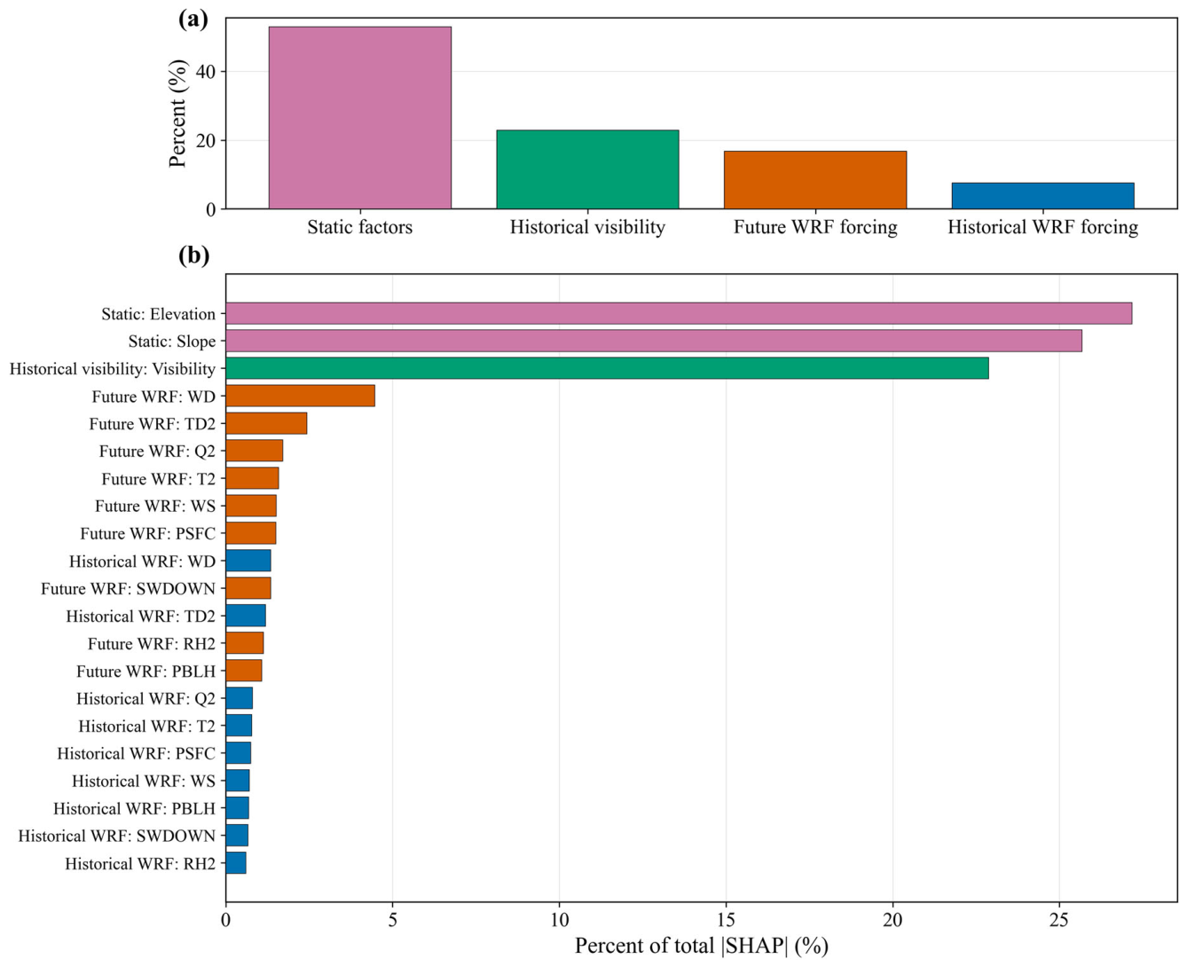
Figure 11 presents the SHAP contributions of the input features. Among the four input branches, static variables accounted for the largest contribution, approximately 54%, followed by historical visibility and future WRF forecasts, which contributed approximately 23% and 16%, respectively. Historical WRF meteorological fields accounted for approximately 7%. Elevation and slope were the most influential static features, indicating that the complex terrain of Guizhou plays an important role in the spatial variability of visibility. Terrain affects the formation and distribution of low visibility by regulating local moisture convergence, cold-air pooling, and boundary-layer conditions. Historical visibility also made a substantial contribution, reflecting the persistence and state dependence of low-visibility events [33].

Figure 11. Statistical analysis of feature contributions in the MS-WRF-ConvLSTM model. Panel (a) shows the contributions of the four input branches, and panel (b) shows the contributions of the individual input features.

Among the WRF meteorological variables, wind direction made a relatively large contribution in both the future and historical meteorological fields. Thermodynamic and moisture-related variables, including 2-m dew-point temperature, 2-m specific humidity, and 2-m air temperature, were also important. These results indicate that the model considers not only local temperature and moisture conditions but also information related to airflow transport and topographic pathways. Over the mountainous terrain of Guizhou, changes in wind direction can alter moisture transport pathways, valley ventilation, and the locations of cold-air convergence, thereby affecting the formation and spatial evolution of low-visibility events [41]. The SHAP analysis demonstrates that MS-WRF-ConvLSTM identifies terrain, thermodynamic, moisture, and transport-related features associated with the formation and evolution of low visibility over Guizhou. This physical plausibility further supports the model’s applicability to spatiotemporal visibility forecasting over complex terrain.

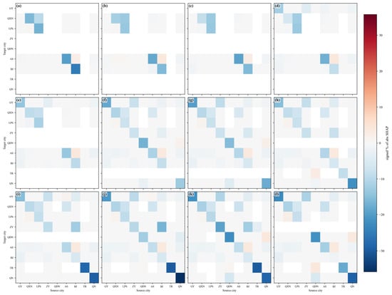
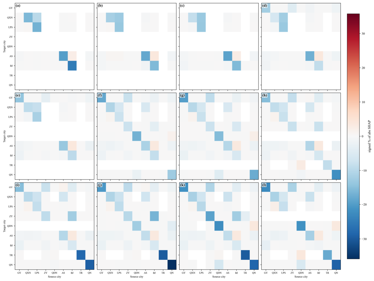
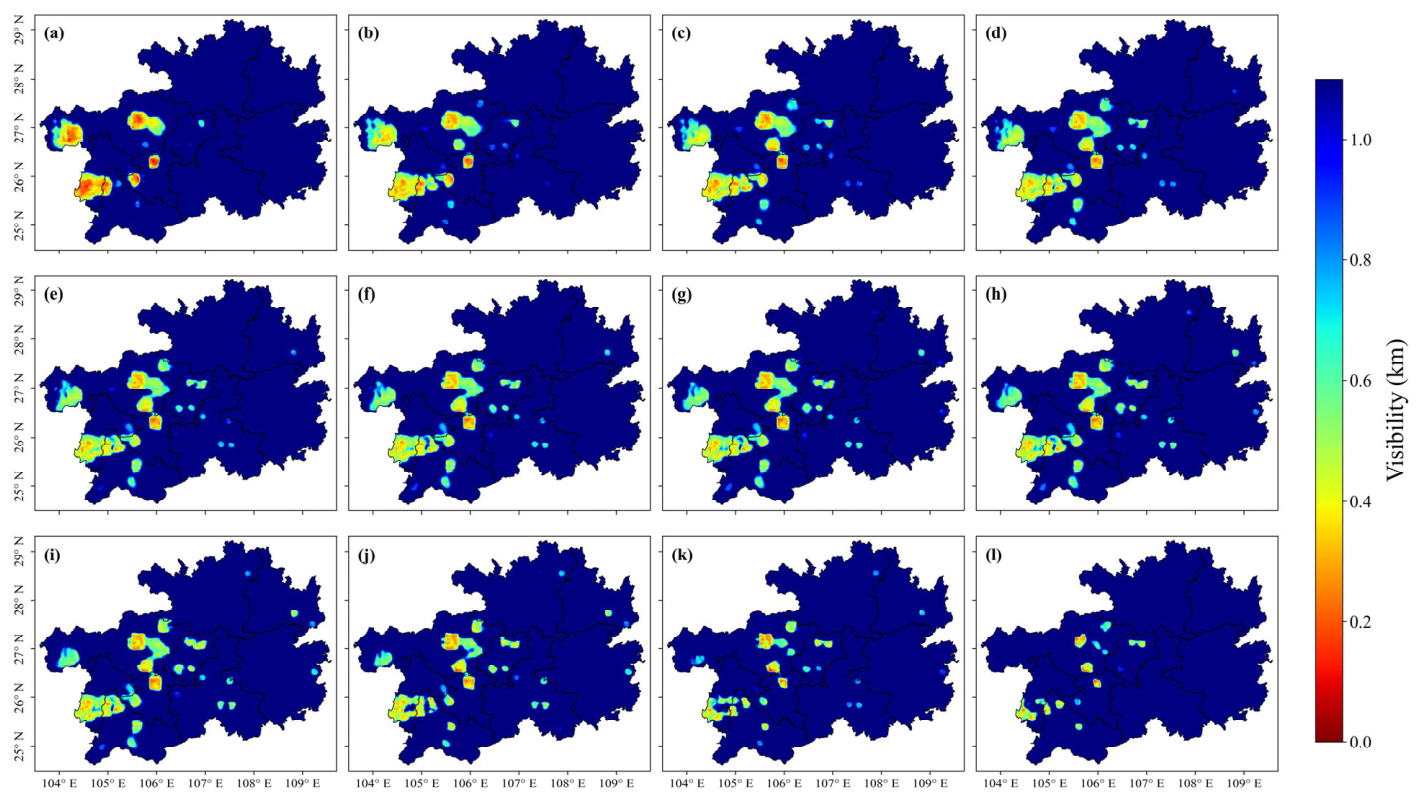
To further examine the spatial forecasting capability of MS-WRF-ConvLSTM, a typical event initialized at 16:00 on 8 December 2024 was selected, and SHAP contribution analysis was conducted at the administrative-region scale (Figure 12). During the early forecast period, contributions from most cities were predominantly negative, indicating that historical information mainly reduced the predicted visibility. This pattern shows that the model captured the persistence of the low-visibility event. As forecast lead time increased, positive contributions from some city pairs gradually increased after approximately the seventh forecast hour, consistent with the gradual contraction of the low-visibility area shown in Figure 13h–l.

Figure 12. Heatmaps of regional-scale feature contributions. Panels (a–l) correspond to forecast lead times of 1–12 h, respectively.

Figure 13. Twelve-hour visibility forecasts initialized at 16:00 on 8 December 2024. Panels (a–l) correspond to forecast lead times of 1–12 h, respectively.

The strongest spatial contributions were mainly concentrated near the diagonal of the heatmap, indicating that predictions for each target city largely depended on its own historical state. This result demonstrates the model’s effective use of local persistence information. However, notable contributions also appeared in some off-diagonal regions, including the positive contribution from BJ to AS at forecast hour 1 and the negative contribution from LPS to QXN at forecast hour 2. These patterns indicate that the model uses historical relationships among different regions rather than relying solely on the characteristics of each target city. Therefore, MS-WRF-ConvLSTM can learn cross-regional spatial dependencies and represent spatial associations in visibility variations over the complex terrain of Guizhou.

It should be noted that spatial SHAP contributions represent the relative influence of regional input information on model predictions and do not necessarily correspond to actual atmospheric transport processes. They are therefore used only as supporting evidence for evaluating the model’s ability to learn spatial associations and should not be directly interpreted as physical propagation pathways of low visibility.

4. Discussion

4.1. Role of the Coarse-to-Fine Framework in Visibility Forecasting over Complex Terrain

The multiscale forecasting model developed in this study decomposes large-area visibility forecasting into two stages: coarse-scale spatiotemporal prediction and fine-scale spatial reconstruction. It therefore does not improve forecasting performance merely by increasing the resolution of the input data. The ablation experiments showed that the coarse-scale model achieved high numerical accuracy at a relatively low spatial resolution but inadequately represented local low-visibility centers and their surrounding details. After CVIS prior information was introduced into the fine-scale reconstruction, the model recovered more local spatial structures while retaining the overall evolution of the visibility field. This framework reduces the computational cost of direct long-sequence, large-area, high-resolution forecasting while maintaining relatively high visibility prediction accuracy. WRF-LSTM mainly predicts individual-pixel time series and consequently produces relatively scattered forecast fields. In contrast, MS-WRF-ConvLSTM uses spatial relationships among neighboring regions, resulting in more stable correlations and error levels across the prefecture-level regions of Guizhou. For Guizhou, where terrain varies markedly and low-visibility events are highly localized, this coarse-to-fine task decomposition captures both regional-scale evolution and local-scale spatial differences. This capability is the main reason why the multiscale model outperforms the single-pixel time-series model.

4.2. Roles of the CVIS Physical Spatial Prior and High-Temporal-Resolution WRF Forecast Fields

Analysis of the spatial differences among the ablation schemes showed that Scheme 1 achieved relatively high numerical forecasting accuracy but produced outputs at a coarse spatial resolution. It therefore could not fully represent local differences and fine-scale structures in low-visibility fields over complex terrain, requiring spatial downscaling to obtain high-resolution forecasts. Schemes 2 and 3 both reconstructed fine-scale fields from coarse-scale predictions but differed in whether the CVIS spatial constraint was included. Scheme 2 used the CVIS-derived visibility field as a prior for local spatial distributions, providing an explicit constraint for fine-scale reconstruction. Consequently, it maintained a relatively high correlation and markedly outperformed Scheme 3, which did not include this constraint. Notably, the main value of the CVIS field lies not in its direct numerical forecasting accuracy but in the physically meaningful spatial patterns it provides for fine-scale reconstruction. When used independently for visibility diagnosis, CVIS showed low correlations and large errors relative to station observations. However, incorporating its spatial distribution into the fine-scale model substantially improved performance compared with Scheme 3. Spatial comparisons also showed that removing the CVIS constraint weakened some local high- and low-value centers and spatial gradients. WRF meteorological fields alone are therefore insufficient to fully represent local visibility variations over complex terrain, whereas CVIS provides additional high-resolution spatial prior information. This prior does not replace the model prediction but guides the model during training to learn spatial patterns consistent with the observations, thereby improving the representation of local structures and fine-scale features while preserving the overall evolution of the visibility field.

Scheme 5 used WRF meteorological fields with a lower temporal resolution and showed a marked decrease in visibility forecasting accuracy compared with Scheme 2. Its ability to represent local details also weakened, and some rapidly changing areas exhibited spatial smoothing. These results indicate that high-temporal-resolution meteorological forcing provides richer information on dynamic variations and helps the model capture the rapid evolution of visibility.

Overall, the CVIS spatial prior and high-temporal-resolution WRF meteorological forcing play complementary roles. CVIS is derived from WRF thermodynamic and moisture-related variables and provides a high-resolution reference for local spatial structures, whereas the 10-min WRF meteorological fields provide denser information on spatiotemporal evolution.

5. Conclusions

A multisource dataset was constructed using WRF meteorological fields, station-based visibility observations, and static geographical data from 2022 to 2024. Based on the ConvLSTM architecture, a multiscale joint forecasting model centered on coarse-scale spatiotemporal prediction and fine-scale spatial reconstruction was developed to generate spatially continuous, high-resolution visibility forecasts over Guizhou Province for the subsequent 12 h. Model performance was evaluated using typical low-visibility events, and SHAP analysis was applied to examine the importance of input features and intercity contribution patterns. The main conclusions are as follows:

• MS-WRF-ConvLSTM improved the forecasting accuracy of low-visibility events. On the 2024 validation dataset, it outperformed WRF-LSTM in both numerical and categorical forecasting, achieving R values of 0.59–0.73 and RMSE values of 0.81–1.01 km. For the VIS ≤ 200 m, VIS ≤ 500 m, and VIS ≤ 1000 m categories, MS-WRF-ConvLSTM produced higher hit rates and more stable TS values. Its BS values were generally close to 1, indicating that the predicted frequency of severe low-visibility events was closer to the observations and demonstrating more balanced event identification and greater stability across forecast lead times.
• MS-WRF-ConvLSTM showed stable and comprehensive performance at the prefecture level and in predicting spatial distributions. Its regional R and RMSE values were consistently better than those of WRF-LSTM. Higher TS and BS values, mainly within 0.9–1.5 across visibility categories, indicate a better balance among hits, misses, and false alarms. In addition, the ConvLSTM representation of spatial relationships among neighboring pixels enhanced the continuity and local detail of the predicted fields, producing distributions closer to the station-interpolated fields and making the model more suitable for refined visibility forecasting over complex terrain.
• The ablation experiments confirmed the effectiveness of the multiscale architecture, high-temporal-resolution meteorological data, and CVIS spatial constraint. High-temporal-resolution inputs improved the model’s ability to represent the rapid evolution of low visibility. Although the coarse-scale model achieved relatively high numerical accuracy, its spatial resolution was limited. Introducing the CVIS constraint enabled high-resolution spatial reconstruction while maintaining relatively high correlations and markedly improved performance compared with the unconstrained scheme. Despite the limited direct prediction accuracy of CVIS, its physically based spatial prior improved the representation of local low-visibility distributions and provided a better balance between forecasting accuracy and fine-scale spatial detail.
• SHAP analysis showed that MS-WRF-ConvLSTM effectively integrated terrain, historical visibility, and meteorological information. Static variables made the largest contribution, accounting for approximately 54%, while elevation, slope, historical visibility, and wind direction were among the most important features. The model also learned spatial associations among different cities, demonstrating its ability to represent spatiotemporal visibility variations over the complex terrain of Guizhou.

References

- Hyslop, N.P. Impaired visibility: The air pollution people see. Atmos. Environ. 2009, 43, 182–195. [Google Scholar] [CrossRef] [Scilit]
- Hu, J.; Sun, S.; Wang, R. Research on the influence of light source characteristics on traffic visual distance in foggy areas at night. Build. Environ. 2022, 212, 108818. [Google Scholar] [CrossRef] [Scilit]
- He, D.; Wang, Y.; Tang, Y.; Kong, D.; Yang, J.; Zhou, W.; Li, H.; Wang, F. Improvement in the Forecasting of Low Visibility over Guizhou, China, Based on a Multi-Variable Deep Learning Model. Atmosphere 2024, 15, 752. [Google Scholar] [CrossRef] [Scilit]
- Weston, M.J.; Piketh, S.J.; Burnet, F.; Broccardo, S.; Denjean, C.; Bourrianne, T.; Formenti, P. Sensitivity analysis of an aerosol-aware microphysics scheme in Weather Research and Forecasting (WRF) during case studies of fog in Namibia. Atmos. Chem. Phys. 2022, 22, 10221–10245. [Google Scholar] [CrossRef] [Scilit]
- Long, Q.; Wu, B.; Mi, X.; Liu, S.; Fei, X.; Ju, T. Review on parameterization schemes of visibility in fog and brief discussion of applications performance. Atmosphere 2021, 12, 1666. [Google Scholar] [CrossRef] [Scilit]
- Kunkel, B.A. Parameterization of droplet terminal velocity and extinction coefficient in fog models. J. Appl. Meteorol. Climatol. 1984, 23, 34–41. [Google Scholar] [CrossRef] [Scilit]
- Doran, J.; Roohr, P.; Beberwyk, D.; Brooks, G.; Gayno, G.; Williams, R.; Lewis, J.; Lefevre, R. The MM5 at the Air Force Weather Agency-New products to support military operations. In Proceedings of the 8th Conference on Aviation, Range, and Aerospace Meteorology, Dallas, TX, USA, 10–15 January 1999. [Google Scholar]
- Won, W.-S.; Oh, R.; Lee, W.; Kim, K.-Y.; Ku, S.; Su, P.-C.; Yoon, Y.-J. Impact of fine particulate matter on visibility at incheon international airport, South Korea. Aerosol Air Qual. Res. 2020, 20, 1048–1061. [Google Scholar] [CrossRef] [Scilit]
- Peláez-Rodríguez, C.; Pérez-Aracil, J.; de Lopez-Diz, A.; Casanova-Mateo, C.; Fister, D.; Jiménez-Fernández, S.; Salcedo-Sanz, S. Deep learning ensembles for accurate fog-related low-visibility events forecasting. Neurocomputing 2023, 549, 126435. [Google Scholar] [CrossRef] [Scilit]
- Zhu, L.; Zhu, G.; Han, L.; Wang, N. The application of deep learning in airport visibility forecast. Atmos. Clim. Sci. 2017, 7, 314. [Google Scholar]
- Lu, Z.; Zheng, C.; Yang, T. Application of offshore visibility forecast based on temporal convolutional network and transfer learning. Comput. Intell. Neurosci. 2020, 2020, 8882279. [Google Scholar] [CrossRef] [Scilit] [PubMed]
- Peláez-Rodríguez, C.; Pérez-Aracil, J.; Casanova-Mateo, C.; Salcedo-Sanz, S. Efficient prediction of fog-related low-visibility events with Machine Learning and evolutionary algorithms. Atmos. Res. 2023, 295, 106991. [Google Scholar] [CrossRef] [Scilit]
- Gu, L.-M.; Zeng, X.-M.; Li, C.-M.; Wang, N.; Shao, S.-B.; Ullah, I. A numerical simulation of a fog event in the Sichuan basin, china: The sensitivity to terrain elevations. Atmosphere 2024, 15, 1546. [Google Scholar] [CrossRef] [Scilit]
- Yu, L.; Zhuge, X.; Yuan, W.; Gao, N.; Li, J.; Fu, Y.; Chen, F.; Yao, B.; Tang, F.; Kan, W. Cloud characteristics over the Yunnan-Guizhou plateau as observed by MODIS and Himawari-8. Int. J. Climatol. 2023, 43, 8072–8085. [Google Scholar] [CrossRef] [Scilit]
- Pu, Z.; Pardyjak, E.R.; Hoch, S.W.; Gultepe, I.; Hallar, A.G.; Perelet, A.; Beal, R.; Carrillo-Cardenas, G.; Li, X.; Garcia, M. Cold fog amongst complex terrain. Bull. Am. Meteorol. Soc. 2023, 104, E2030–E2052. [Google Scholar] [CrossRef] [Scilit]
- Farr, T.G.; Kobrick, M. Shuttle Radar Topography Mission produces a wealth of data. Eos Trans. Am. Geophys. Union 2000, 81, 583–585. [Google Scholar] [CrossRef] [Scilit]
- Zhu, W.; Yang, J.; Zhang, Y.; Du, X.; Li, L.; Qi, D. Effect of Refined WRF Static Data on Simulation of Quasi-stationary Front Frontal Fog. Plateau Mt. Meteorol. Res. 2024, 44, 81–89. [Google Scholar] [CrossRef]
- Bang, C.-H.; Lee, J.-W.; Hong, S.-Y. Predictability experiments of fog and visibility in local airports over Korea using the WRF model. J. Korean Soc. Atmos. Environ. 2008, 24, 92–101. [Google Scholar]
- Gao, R.; Li, X.; Shi, X. Comparative study on three algorithms of the visibility in Qingdao offshore areas based on WRF model. J. Mar. Meteorol. 2018, 38, 28–35. [Google Scholar]
- Qiao, X.; Guo, H.; Tang, Y.; Wang, P.; Deng, W.; Zhao, X.; Hu, J.; Ying, Q.; Zhang, H. Local and regional contributions to fine particulate matter in the 18 cities of Sichuan Basin, southwestern China. Atmos. Chem. Phys. 2019, 19, 5791–5803. [Google Scholar] [CrossRef] [Scilit]
- Dai, X.; Wang, J.; Wu, C.; Wan, C.; Liu, Z.; Li, Y.; Ye, F.; Zhang, Y. Spatially comprehensive estimation of hourly PM2.5 concentration in a cloud-covered basin based on remote sensing and meteorological models. Atmos. Environ. 2025, 359, 121374. [Google Scholar] [CrossRef] [Scilit]
- Xian, Y.; Zhang, Y.; Liu, Z.; Wang, H.; Xiong, T. Characterization of winter PM2.5 source contributions and impacts of meteorological conditions and anthropogenic emission changes in the Sichuan Basin, 2002–2020. Sci. Total Environ. 2024, 947, 174557. [Google Scholar] [CrossRef] [Scilit] [PubMed]
- Emery, C.; Liu, Z.; Russell, A.G.; Odman, M.T.; Yarwood, G.; Kumar, N. Recommendations on statistics and benchmarks to assess photochemical model performance. J. Air Waste Manag. Assoc. 2017, 67, 582–598. [Google Scholar] [CrossRef] [Scilit] [PubMed]
- Rzeszutek, M.; Kłosowska, A.; Oleniacz, R. Accuracy assessment of WRF model in the context of air quality modeling in complex terrain. Sustainability 2023, 15, 12576. [Google Scholar] [CrossRef] [Scilit]
- Hou, T.; Yu, S.; Jiang, Y.; Chen, X.; Zhang, Y.; Li, M.; Li, Z.; Song, Z.; Li, P.; Chen, J. Impacts of chemical initial conditions in the WRF-CMAQ model on the ozone forecasts in eastern China. Aerosol Air Qual. Res. 2022, 22, 210402. [Google Scholar] [CrossRef] [Scilit]
- Li, J.; Yu, S.; Chen, X.; Zhang, Y.; Li, M.; Li, Z.; Song, Z.; Liu, W.; Li, P.; Xie, M. Evaluation of the WRF-CMAQ model performances on air quality in China with the impacts of the observation nudging on meteorology. Aerosol Air Qual. Res. 2022, 22, 220023. [Google Scholar] [CrossRef] [Scilit]
- Ebert, E.E. Fuzzy verification of high-resolution gridded forecasts: A review and proposed framework. Meteorol. Appl. A J. Forecast. Pract. Appl. Train. Tech. Model. 2008, 15, 51–64. [Google Scholar] [CrossRef] [Scilit]
- Zhu, K.; Yu, B.; Xue, M.; Zhou, B.; Hu, X.M. Summer season precipitation biases in 4 km WRF forecasts over southern China: Diagnoses of the causes of biases. J. Geophys. Res. Atmos. 2021, 126, e2021JD035530. [Google Scholar] [CrossRef] [Scilit]
- Zhang, J.; Zhao, P.; Wang, X.; Zhang, J.; Liu, J.; Li, B.; Zhou, Y.; Wang, H. Main factors influencing winter visibility at the xinjin flight college of the civil aviation flight university of China. Adv. Meteorol. 2020, 2020, 8899750. [Google Scholar] [CrossRef] [Scilit]
- Luan, T.; Guo, X.; Guo, L.; Zhang, T. Quantifying the relationship between PM 2.5 concentration, visibility and planetary boundary layer height for long-lasting haze and fog-haze mixed events in Beijing. Atmos. Chem. Phys. 2018, 18, 203–225. [Google Scholar] [CrossRef] [Scilit]
- Liu, N.; Luo, T.; Han, Y.; Yang, K.; Zhang, K.; Wu, Y.; Weng, N.; Li, X. Analysis of the atmospheric visibility influencing factors under sea-land breeze circulation. Opt. Express 2022, 30, 7356–7371. [Google Scholar] [CrossRef] [Scilit] [PubMed]
- Lal, A.K.; Kunchala, R.K.; Mohan, M. Impact of Land Use Land Cover (LULC) on the physical processes of a dense fog episode: A case study using WRF model from the National Capital Region, India. Atmos. Environ. 2025, 343, 121014. [Google Scholar] [CrossRef] [Scilit]
- Dietz, S.J.; Kneringer, P.; Mayr, G.J.; Zeileis, A. Low-visibility forecasts for different flight planning horizons using tree-based boosting models. Adv. Stat. Climatol. Meteorol. Oceanogr. 2019, 5, 101–114. [Google Scholar] [CrossRef] [Scilit]
- Bi, K.; Xie, L.; Zhang, H.; Chen, X.; Gu, X.; Tian, Q. Accurate medium-range global weather forecasting with 3D neural networks. Nature 2023, 619, 533–538, Correction in Nature 2023, 621, E45. [Google Scholar] [CrossRef] [Scilit] [PubMed]
- Johnson, J.M.; Khoshgoftaar, T.M. Survey on deep learning with class imbalance. J. Big Data 2019, 6, 27. [Google Scholar] [CrossRef] [Scilit]
- Li, X.; Pu, Z. Turbulence effects on the formation of cold fog over complex terrain with large-eddy simulation. Geophys. Res. Lett. 2022, 49, e2022GL098792. [Google Scholar] [CrossRef] [Scilit]
- Boutle, I.; Finnenkoetter, A.; Lock, A.; Wells, H. The London Model: Forecasting fog at 333 m resolution. Q. J. R. Meteorol. Soc. 2016, 142, 360–371. [Google Scholar] [CrossRef] [Scilit]
- Song, J.I.; Yum, S.S.; Gultepe, I.; Chang, K.-H.; Kim, B.-G. Development of a new visibility parameterization based on the measurement of fog microphysics at a mountain site in Korea. Atmos. Res. 2019, 229, 115–126. [Google Scholar] [CrossRef] [Scilit]
- Jayakumar, A.; Rajagopal, E.; Boutle, I.A.; George, J.P.; Mohandas, S.; Webster, S.; Aditi, S. An operational fog prediction system for Delhi using the 330 m Unified Model. Atmos. Sci. Lett. 2018, 19, e796. [Google Scholar] [CrossRef] [Scilit]
- Lundberg, S.M.; Lee, S.-I. A unified approach to interpreting model predictions. Adv. Neural Inf. Process. Syst. 2017, 30, 4768–4777. [Google Scholar]
- Yan, S.; Wang, H.; Liu, X.; Zu, F.; Liu, D. Effect of the boundary layer low-level jet on fast fog spatial propagation. Atmos. Chem. Phys. 2023, 23, 13987–14002. [Google Scholar] [CrossRef] [Scilit]
Disclaimer/Publisher’s Note: The statements, opinions and data contained in all publications are solely those of the individual author(s) and contributor(s) and not of MDPI and/or the editor(s). MDPI and/or the editor(s) disclaim responsibility for any injury to people or property resulting from any ideas, methods, instructions or products referred to in the content. |
© 2026 by the authors. Licensee MDPI, Basel, Switzerland. This article is an open access article distributed under the terms and conditions of the Creative Commons Attribution (CC BY) license.