


Highlights
What are the main findings?
- A Student-t copula with Student-t marginals removes both the thin marginal tails and the zero tail dependence inherent in the Gaussian Cholesky innovations of the Society of Actuaries liability-driven-investment scenario generator, sharpening extreme-risk estimates while leaving central projections unchanged; it is a more general form of the benchmark, of which the Gaussian model is a special case.
- Relative to this copula specification, the Gaussian benchmark understates 99% expected-shortfall capital by about 11%, a shortfall whose direction is robust across bootstrap resampling.
What are the implications of the main findings?
- Gaussian scenario generators can materially understate capital requirements under joint yield–currency stress, which a Student-t copula corrects by capturing the extreme co-movements that Gaussian dependence omits.
- The framework transfers to any market with monthly data and supports reproducible expected-shortfall capital and regulatory scenario analysis under IFRS 17 and Basel III.
Abstract
Pension funds and insurers in emerging markets size long-horizon capital with economic scenario generators (ESGs)—econometrically, simulators of a multivariate predictive density. The production benchmark draws its innovations by Gaussian Cholesky factorization, forcing thin marginal tails and zero joint tail dependence, so it cannot generate the simultaneous yield and currency shocks that dominate emerging-market stress; as supervisors move market-risk capital to expected shortfall, a density blind to joint extremes understates the number they now act on. We retain the three-layer liability-driven-investment cascade but replace its innovation engine with a Student-t copula over Student-t marginals, a more general specification of which the Gaussian benchmark is a special case, and validate it on Indonesian data from February 2010 to May 2026. A boundary-corrected bootstrap test rejects the Gaussian dependence structure; the heavy-tailed engine is the better-calibrated joint density forecast both in sample and in real-time rolling evaluation, with a scoring advantage that is clear in sample and small in real time; and the Gaussian default understates 99% expected-shortfall capital by about 11%, a direction that is robust across bootstrap resamples and across truncation and tail-heaviness settings, though imprecise in magnitude. Framed as a density forecast and judged by calibration and proper scores, the copula engine is better calibrated and more prudent, pricing the joint extremes the Gaussian default omits.
1. Introduction
Emerging-market economies face tightly coupled sources of financial risk, shaped by global business cycles, commodity-price swings, capital-flow reversals, and domestic structural frictions [1]. For insurers, pension funds, and other liability-driven investors, these conditions complicate capital planning and asset–liability management over multi-year horizons [2], and they bind hardest where structural change, policy intervention, and macroeconomic volatility run highest [3]. Regulation has moved in the same direction. Basel III and the Fundamental Review of the Trading Book shift market-risk capital from value-at-risk (VaR) to expected shortfall (ES), precisely to capture losses beyond the VaR threshold [4]. Solvency II and IFRS 17, in turn, require insurers to value liabilities and capital under adverse but plausible forward-looking scenarios rather than historical averages [5,6]. A generator that cannot produce joint tail events understates the expected shortfall these regimes now mandate.
Economic scenario generators (ESGs) are the field’s response. An ESG produces internally consistent stochastic projections of macroeconomic variables, interest rates, and asset returns under one probabilistic structure, supporting stress testing, capital allocation, and long-horizon investment analysis [7,8]. In econometric language, an ESG is a device for multivariate density forecasting: conditional on the information set, it characterizes the joint predictive distribution of future states, and its Monte Carlo paths are draws from that density rather than deterministic point forecasts [9,10]. This reframing matters because the object a supervisor or LDI manager ultimately acts on, expected-shortfall capital, is a nonlinear functional of the tail of that joint density. A model can forecast the conditional mean well and still misprice capital if its predictive density carries the wrong tail. The natural tools for judging an ESG are therefore those of density-forecast evaluation: the probability integral transform for calibration [11], and proper scoring rules for the joint distribution and its tails [12,13,14].
A widely adopted design principle in modern ESGs is hierarchical consistency, in which macroeconomic variables serve as the primary stochastic drivers and asset models are specified conditionally on them. This principle is formalized in the Society of Actuaries’ Liability-Driven Investment Benchmark Model, a modular ESG anchored by a macroeconomic core and complemented by asset and liability modules [7]. The benchmark, like most production cascades, draws its innovations by Gaussian Cholesky factorization: with , where L is the Cholesky factor of the innovation covariance. That single device is a joint distributional assumption because it imposes Gaussian marginals and a Gaussian copula. The Gaussian marginals restrict every shock to thin tails. The Gaussian copula has zero asymptotic tail dependence: as McNeil, Frey, and Embrechts [8] show, the probability that two variables are extreme together vanishes in the tail, however strong their correlation. In advanced markets, these restrictions are questionable; in emerging markets, where heavy-tailed innovations and clustered joint extremes are common [1,15,16], they are difficult to defend. The literature repairs the two failures separately, in three strands that this paper joins. The first replaces the marginal law: heavy-tailed VAR innovations and regime-switching designs [17] address marginal tails and time-varying volatility but leave the Gaussian dependence intact. The second models dependence directly. Copulas are standard in market-risk aggregation [18,19] and have been applied recently to emerging-market energy and equity portfolios [20,21], and the family extends to pair-copula constructions [22] and skew-elliptical laws [23]; these models are usually fitted to asset returns alone rather than inside a scenario cascade with a stress layer, a yield-curve mapping and a liability metric. The third strand supplies the evaluation standard: calibration by the probability integral transform [11] and sharpness by proper scoring rules [12,13], applied to macroeconomic and financial forecasts [9,10] but rarely to actuarial scenario generators. The common industry remedy, swapping Gaussian draws for unit-variance Student-t draws, addresses only marginals, and we show its effect on tail quantiles reverses sign with the reporting level. No existing emerging-market ESG repairs both failures inside an architecture practitioners already use and prices the repair in regulatory capital evaluated as a density forecast. This is the gap, and the contribution combines the three strands: a heavy-tailed copula engine inside the cascade practitioners already run, tested against its Gaussian boundary and judged as a density forecast.
This study builds and validates exactly that engine and applies it to Indonesia, a representative emerging market. Indonesia has an active inflation-targeting central bank, a deepening local-currency government bond market that is heavily foreign-held and therefore sensitive to global risk appetite, and pronounced commodity and currency exposure. These features concentrate the joint yield–currency tail risk the framework targets [3]. We retain the three-layer cascade, augment its conditional-mean layer with an optional stationary error-correction term that preserves a long-run yield-curve equilibrium (a feature the Indonesian curve exhibits over the sample), and replace the innovation engine with a Student-t copula over Student-t marginals fitted at their estimated scale. The framework nests three engines, the SoA-Gaussian benchmark (M1), a marginal-t intermediate (M2), and the full t-copula (M3), which are three competing density forecasts whose capital gap decomposes exactly into a marginal part (M1→M2) and a dependence part (M2→M3). A Student-t marginal and a t-copula both reduce to their Gaussian counterparts as their degrees of freedom grow. The construction is therefore a strict generalization of the benchmark, not an alternative to it: it reproduces the Gaussian generator when the innovations are light-tailed and tail-independent and departs from it only when the data show heavy tails or joint extremes. Adopting it is, in this sense, conservative.
This paper is intentionally positioned at the boundary between actuarial economic scenario generation and econometric density forecasting. The three-layer cascade is actuarial in origin because its purpose is LDI capital measurement rather than short-horizon point prediction; the contribution, however, is econometric. We replace the Gaussian Cholesky innovation law with an estimable heavy-tailed copula density, test the Gaussian copula against a boundary alternative, preserve cointegrating yield-curve structure through an error-correction term, and evaluate the resulting predictive distribution by probability-integral-transform calibration, a proper multivariate scoring rule, and expected-shortfall capital. The vector autoregression (VAR) and the stress logit are therefore not presented as novel forecasting models; they are transparent conditional-mean and stress-labelling layers within which the distributional innovation is isolated and priced.
Four contributions follow. First, we formulate the ESG as a multivariate density forecast and make the innovation distribution, not the conditional mean, the object of evaluation (Section 2 and Section 2.5). Second, we provide three analytic results that motivate the design: a standardization compression factor, an exact quantile-ratio characterization of when the unit-variance overlay backfires, and the strict positivity of t-copula tail dependence at every finite degree of freedom (Section 3); these are not new distributional theory but tail-risk diagnostics that bear directly on capital. Third, we validate on 196 months of real, un-interpolated Indonesian data, quantifying the Gaussian engine’s capital understatement at about 11% at the point estimate, reporting its bootstrap distribution, and evaluating the engines as density forecasts both in sample and in real-time rolling evaluation at one-, twelve- and twenty-four-month horizons, where the t-copula is the better-calibrated forecast (Section 4). Fourth, we give a six-step implementation protocol that transfers the framework to any jurisdiction with monthly market data (Section 2.6). Section 5 discusses implications and limitations, and Section 6 concludes this paper.
2. Methodology
We present a general three-layer economic scenario generator and isolate its innovation distribution as the object of study. The framework is specified for an arbitrary collection of macro-financial variables; the variables used in the empirical study and the justification for choosing them are deferred to Section 4 so that the model is motivated on theoretical rather than data-specific grounds. The construction follows the hierarchical principle of the Society of Actuaries liability-driven-investment (LDI) Benchmark Model [7]: a macro-financial block is the primary stochastic driver, and a stress-regime layer and an asset and yield-curve mapping are specified conditionally on it. This section sets out the three layers and their dependencies, the innovation engine that is the paper’s contribution, and the estimation and validation protocol; every symbol is defined at first use, together with its unit.
2.1. State Vector and the Three-Layer Architecture
Let denote the macro-financial state vector in period t, a column vector of K variables each rendered stationary by an appropriate transform: a first difference for a level series, a log return for a price series, or a growth rate for a flow. Every component is therefore a stationary, mean-reverting quantity expressed in its own natural unit, for example, a yield change in basis points or an asset log return in percent. A fixed selection matrix () extracts a named coordinate so that is the j-th component of . The three layers form a recursive chain: Layer 1 generates the state, Layer 2 reads a stress-regime label off the state, and Layer 3 maps the state to the observable term structure and asset prices.
Layer 1: state dynamics. The conditional mean of the state follows a first-order vector autoregression, optionally augmented by a stationary error-correction term that encodes a long-run economic relationship among the underlying levels, i.e.,
Here, is an intercept vector in the units of ; is the (dimensionless) autoregressive coefficient matrix, whose entry is the one-period response of variable i to variable j; is a scalar error-correction term, a stationary, mean-zero combination of lagged levels that is positive when the long-run relationship is stretched in one direction and negative in the other; is the vector of speed-of-adjustment loadings, in units of x per unit of ; and is a zero-mean innovation vector, in units of , with a contemporaneous joint distribution (). Equation (1) has two structural parts: a first-order vector-autoregressive term () for the conditional mean and an error-correction term () for long-run structure among the levels. The vector autoregression is the standard reduced-form model for the joint conditional mean of a macro-financial system, as developed by Lütkepohl [24]; it places no exclusion restrictions on contemporaneous interactions and coincides with the linear projection of the state on its own past. The error-correction term encodes cointegration, a stable long-run equilibrium among non-stationary levels. We retain it for a specific reason: when the levels share a long-run equilibrium, differencing each one separately discards that information, whereas reintroduces it and pulls the system back toward equilibrium [24]. Setting removes the term and recovers the pure first-difference VAR of the production benchmark. The distribution () of is left unspecified here and is the subject of Section 2.2. Because the conditional mean is linear, it is tail-neutral, so alone governs the tail behaviour of the generated scenarios.
Layer 2: stress-regime label. Conditional on the state, a binary stress regime (, with denoting a stress period) has an occurrence probability given by a logistic model in lagged leading indicators that are, themselves, functions of the Layer-1 state, i.e.,
Here, is the conditional stress probability; is a vector of m leading indicators observable at and reconstructed from the state path, each in its own unit; is an intercept on the log-odds scale; is the coefficient vector, in log-odds per unit of the corresponding indicator; is the logistic link mapping the linear index to a probability; and is the information set at . Equation (2) specifies the stress regime as a logistic model whose linear index is built from lagged leading indicators (). We use financial leading indicators—specifically, the slope of the yield curve and a measure of financial volatility—for an established reason. Estrella and Mishkin [25] and Kauppi and Saikkonen [26] find these variables to be among the most robust predictors of subsequent economic stress. The term spread is informative because it embeds market expectations of future short rates and the monetary-policy stance. Layer 2 is conditional on Layer 1 and introduces no new stochastic driver. It attaches a stress probability and, hence, a regime label, to each already-simulated state path, and the cascade uses that label for regime-dependent reporting rather than for generation of the state.
Layer 3: asset and yield-curve mapping. Conditional on the same simulated state, the observable term structure is reconstructed by an affine factor mapping; the yield at tenor () is affine in a small number of curve factors:
Equation (3) represents each tenor yield as an affine function of a small number of common curve factors. This affine factor structure is the standard low-dimensional description of the yield curve: Litterman and Scheinkman [27] showed that a few factors interpretable as level, slope, and curvature explain almost all of the variation in observed yields, and the parsimonious parametric form of Nelson and Siegel [28] is built on the same factors. The levels required by in (1) and by the factors in (3) are recovered from the simulated changes by accumulation, i.e., , which closes the recursion.
The three layers play distinct but linked roles. Layer 1 is the only stochastic engine: it generates the state path and is the sole point at which the innovation () and, hence, the entire distributional content of the generator enters. Layer 2 and Layer 3 are deterministic measurement maps of that state: Layer 2 reads a stress-regime probability off it, and Layer 3 reads the observable term structure off it. The dependence therefore runs in one direction, i.e., , so a single innovation draw propagates deterministically into the regime label, and the yield curve and the three layers cannot disagree; they form one internally consistent system rather than three separate models.
Table 1 collects the recurring symbols with their meanings and units for reference.
Table 1.
Notation.
Figure 1 summarizes the architecture and isolates the single object of study. Layer 1 is estimated, and its residuals () are extracted; the innovation engine is the law chosen for those residuals, branching into the Gaussian benchmark (M1), the marginal-t intermediate (M2), and the t-copula (M3). The chosen engine drives a forward simulation of Layer 1, and the layers then run as a chain: Layer 1 → Layer 2 → Layer 3, each consuming the previous layer’s output, so the stress label and the yield curve are deterministic functions of the same simulated state. Only the law of differs across engines; everything downstream is shared, and the simulated paths feed a balance-sheet mapping that returns the expected-shortfall capital and the density-forecast diagnostics.
Figure 1.
The three-layer cascade and the three innovation engines. Layer 1 is estimated, and its residuals () are extracted; the innovation engine is the distribution chosen for those residuals (M1, Gaussian; M2, marginal-t; M3, t-copula), the only component that differs across engines. The chosen engine simulates Layer 1 forward, and the state then passes in sequence through Layer 2 (stress-regime label) and Layer 3 (yield-curve map), feeding the LDI balance-sheet map and the out-of-sample density diagnostics. Formatting conventions: bold text names the object of each block; the dashed rectangle encloses the three interchangeable innovation engines, which are the only components that differ across M1, M2 and M3; and the colours distinguish those engines only.
Figure 2 makes the cascade concrete on the Indonesian data. Panel (a) is the estimated correlation structure of the Layer-1 innovations: the positive yield–currency correlation () and the level–slope link (), together with the equity–currency and oil–currency couplings, are the joint structure the copula must reproduce and that the Gaussian engine flattens in the tail. Panel (b) shows the Layer-2 market-stress probability over the sample; it rises sharply at each flagged episode, the 2013 taper tantrum, the 2015 commodity slump, the 2020 pandemic, and the 2024–2026 episodes, and the area under the ROC curve is . Panel (c) shows a sample of the Layer-3 simulated ten-year-yield scenarios with their median and 5–95% range, propagated through the full conditional-mean dynamics. Panel (d) is the engine comparison that motivates the whole exercise: the model-implied probability that the yield and the currency both land in their joint adverse tail. Both engines sit above the independence benchmark () because they share the correlation, but the t-copula assigns markedly more joint mass deep in the tail— against the Gaussian’s at the level—while the two are closer in the body; this is the dependence channel that the capital results below quantify.
Figure 2.
The fitted three-layer cascade on Indonesian data. (a) Layer 1: correlation matrix of the seven innovations (ten-year yield–exchange rate correlation of and level–slope correlation of ; equity negatively correlated with both yields and the currency). (b) Layer 2: fitted market-stress probability from the logit on the lagged term spread and lagged VIX, with realized stress months (red) and the sample mean (dashed); area under the ROC curve of . (c) Layer 3: t-copula ten-year-yield scenarios with graded percentile bands (1–99%, 5–95%, and 25–75%) and three labelled sample paths (adverse, central, and benign), with observed history running into the May 2026 anchor. (d) Model-implied joint adverse-tail probability that the yield and the currency fall together for the Gaussian and t-copula engines against the independence benchmark (; versus at the level). In panel (c) the grey line is the observed history before the projection origin, now named in the legend. In panel (d) the downward arrows in the axis label denote an adverse move in each variable, the grey bars are the independence benchmark , and every bar carries its value. Panel (d) evaluates each engine under its own fitted dependence, so its Gaussian column uses the Pearson correlation of the innovations (), whereas the joint-tail comparison in Section 4.9 holds the copula correlation fixed at for both engines; the two therefore answer different questions.
2.2. The Innovation Engine
The contribution is the distribution () of the innovation () in (1). According to Sklar’s theorem, this joint law factors into marginal distributions and a copula that couples them (McNeil et al. [8]), and the three engines differ only in that factorization. The benchmark engine (M1) is Gaussian Cholesky: with and , where is the covariance matrix of and L is its lower-triangular Cholesky factor. This is equivalent to Gaussian marginals coupled by a Gaussian copula. Such a copula has a pairwise tail-dependence coefficient of for every pair, where is the limiting probability that one component is extreme, given that another is [8]. The proposed engine (M3) instead draws . The dependence vector ) follows a Student-t copula with a correlation matrix of and copula degrees of freedom of , and each marginal () is Student-t with tail index and scale . The scale () is the maximum-likelihood scale parameter, not the standard deviation; the implied standard deviation is for . We call fitting at scale preservation to contrast it with the common unit-variance overlay, which rescales each marginal to a standard deviation of one and thereby compresses its scale by the factor of Theorem 1. The intermediate engine (M2), with t marginals under a Gaussian copula, turns the framework into an identification device. Writing for the capital functional, the total gap obeys the exact identity of . Because M2 differs from M1 only in the marginals and M3 differs from M2 only in the copula, the first bracket is the marginal-tail contribution, and the second is the dependence contribution. Finally, tail dependence is invariant to marginal transformations, so no marginal correction can close the M2→M3 gap; it is a copula property, quantified for the t-copula in Theorem 2 (Section 3).
2.3. Choice of Dependence Structure: Alternatives and Rationale
The Student-t copula is one of several dependence structures that could replace the Gaussian copula. We set out the alternatives and the reasons for our choice.
Vine (pair-copula) constructions [22] are the most flexible: they build a K-dimensional density from bivariate blocks and allow for a different family, including asymmetric families, for each pair. Here, that flexibility is costly. Each of the 21 pairs needs a family choice that is hard to justify in advance for macro-financial innovations, 196 monthly observations are few for selection and estimation on that scale, and no simple vine reduces to the Gaussian-Cholesky benchmark along a single parameter boundary, so the production model would no longer be nested, and the capital comparison would lose its ceteris paribus reading.
Skew-elliptical families—in particular, the multivariate skew-t [23]—add the tail asymmetry that a symmetric t-copula cannot represent. The residual diagnostics do show moderate skewness (reported in Section 4), and we treat symmetry as a limitation of the specification. We defer the extension for two reasons. The failure of the benchmark documented here is the absence of joint tail mass, which the symmetric t-copula repairs with one parameter, and the two opposite-signed balance sheets of Section 4.9 bracket the direction in which asymmetry could matter, so the sign of the capital result does not depend on tail symmetry.
Regime-switching dependence [17] generates crisis states endogenously and is the natural choice when dependence shifts discretely, but it adds a full parameter set per regime, which a sample of this length cannot support at ; Section 5.5 keeps it as the extension for economies where regime breaks dominate. Dynamic-correlation and time-varying copulas [18] relax the static R. As Section 5.5 argues, the full-sample copula is a conservative summary of a strengthening dependence regime, so the static choice biases the measured capital gap downward rather than upward.
We choose the Student-t copula for four reasons. It nests the production benchmark, since the Gaussian copula is the limit (), so the benchmark can be tested rather than discarded (Section 2.4). It is parsimonious: one parameter governs the joint tail, which suits a 196-month sample. Its tail dependence is available in closed form (Theorem 2), so the capital mechanism can be checked analytically rather than only by simulation, and it has a simple economic reading because a t-copula is a Gaussian copula mixed over a common volatility multiplier, i.e., with : joint extremes arrive through a market-wide shock, which is the mechanism emerging-market crises display.
2.4. Generality: The Benchmark as a Special Case
The proposed engine is strictly more general than the classical Gaussian benchmark and contains it as a special case. The M1 benchmark is recovered exactly from M3 along three boundaries: the conditional mean drops the error-correction term (); each marginal loses its excess kurtosis, since as ; and the dependence loses its tail clustering, since the t-copula converges to the Gaussian copula as , for which the tail-dependence coefficient is according to Theorem 2. Symbolically, , with M2 as the intermediate that relaxes only the marginals. The generalization is, in this sense, conservative: any joint behaviour the benchmark can represent, the proposed engine can also represent at the corresponding boundary parameter values, so adopting it cannot worsen the in-sample fit.
What the proposed engine can represent and the benchmark cannot is the simultaneous arrival of extremes. For any finite , the t-copula assigns strictly positive probability to the joint tail in which two variables are extreme together, whereas the Gaussian copula assigns that event asymptotically zero probability, however strong the pairwise correlation; this is the structural contrast made precise in Theorem 2. Because expected-shortfall capital is a functional of exactly this joint tail, the benchmark’s tail capital is, by construction, insensitive to the severity of admitted joint extremes, while the proposed engine’s is not. Whether the added generality is necessary or merely available is then an empirical question, which Section 4 settles by estimating the degrees of freedom and testing the Gaussian boundary directly.
2.5. Scenario Generation as Multivariate Density Forecasting
Conditional on the information set (), the Layer-1 dynamics in (1), together with the innovation engine, define a multi-step joint predictive density (), and the Monte Carlo paths are draws from this density rather than deterministic forecasts [9,10]. The three engines (M1, M2, and M3) are therefore three competing density forecasts that share a conditional mean and a correlation structure and differ only in the law of the innovations. The downstream capital figure is a nonlinear functional of this joint density: expected shortfall and LDI funding loss depend on joint, multi-period transformations of yields and the exchange rate that no marginal summary recovers. We therefore evaluate the engines on the basis of two complementary criteria. Calibration is assessed by a multivariate probability integral transform (PIT). For each out-of-sample month, we compute the squared Mahalanobis radius () of the realized innovation and rank it among the simulated radii under each engine; a well-calibrated joint forecast then yields uniform PIT values [11]. We also report the univariate PIT on the capital-relevant exchange-rate margin. Sharpness subject to calibration is assessed by a proper scoring rule. For the multivariate forecast, we use the energy score, the multivariate generalization of the continuous ranked probability score [13]; it is strictly proper and rewards a forecast that is both calibrated and concentrated [12]. We prefer it to the multivariate logarithmic score for a practical reason: in dimensions, the log score requires the predictive density, itself, to be estimated from the simulated paths, and that density estimate, rather than the model, then drives the comparison, whereas the energy score is computed directly from the simulated sample and remains strictly proper. The benchmark in every comparison is M1, the Gaussian engine inside the same cascade, so a score difference reflects the innovation law alone, with the conditional mean, the correlation structure and all downstream mappings held fixed. We report the energy score under two norms, Euclidean and Mahalanobis (covariance-standardized), so that the comparison does not depend on the differing scales of the seven variables. We then test the out-of-sample score differential for significance with a Diebold–Mariano test. Coverage backtesting of a single VaR quantile [29] evaluates only one point of the density; the energy score evaluates the entire joint predictive distribution, and a tail-weighted score [14] that upweights large joint yield–currency moves targets the region that drives capital. Section 4.6 reports the PIT, the energy score, its significance, and the tail-weighted comparison.
2.6. Estimation and Validation Protocol
Estimation is two-step and deliberately transparent. (i) Unit-root tests on the yield levels and the spread determine whether a stationary spread-reversion term enters (1). (ii) Layer 1 is estimated by least squares; scale-preserving t marginals are fitted to the residuals by maximum likelihood, with bootstrap intervals for each . (iii) The residuals are mapped to uniforms by their fitted marginal CDFs; the copula correlation (R) is obtained by Kendall- inversion, and the copula degrees of freedom () by profile maximum likelihood, with a bootstrap interval. Specifically, pairwise; R is then projected to the nearest valid correlation matrix by flooring its eigenvalues at and renormalizing the diagonal, and the profile likelihood for is maximized over by bounded scalar optimization. (iv) The Gaussian copula, which sits on the parameter boundary (), is tested by a parametric-bootstrap likelihood ratio because the statistic is not asymptotically [30,31]. (v) The engines are evaluated by in-sample and rolling out-of-sample VaR coverage [29] and by the out-of-sample PIT and energy score (Section 2.5). (vi) M1, M2, and M3 are simulated under stated plausibility bounds, and the capital gap, its M1→M2→M3 decomposition, and its bound sensitivity are reported; a residual bootstrap of the full pipeline (resample the Layer-1 residuals, refit marginals and copula, and recompute capital) gives a confidence interval for the headline understatement that propagates parameter uncertainty, not merely simulation noise. All simulations use named seeds, score comparisons use common random numbers across engines, and every reported number is regenerated end to end by the replication notebook provided as Supplementary Materials. A plausibility bound at level q truncates each simulated innovation at its own model-implied marginal quantiles before the balance-sheet mapping, capping individual draws at an analyst-chosen severity while leaving the dependence structure intact. The full pipeline runs in minutes on a dataset of this size, and the replication notebook regenerates every number and figure end to end. Algorithm 1 states the procedure compactly.
The two steps estimate the marginals first and the copula second, with the fitted marginal CDFs held fixed in the second step. This is the inference-functions-for-margins principle of Joe [32], whose rank-based version is analysed by Genest, Ghoudi and Rivest [33]. The copula estimator stays consistent and asymptotically normal, but its asymptotic variance carries a correction for first-stage estimation error, so likelihood inference that ignores the first stage can be size-distorted. We address this by simulation rather than by an asymptotic correction: the bootstrap null in step (iv) is generated at the level of the raw residuals, and the whole two-step procedure is re-estimated on every null sample, so the null distribution contains the first-stage error. Section 4.5 reports that null distribution and a check on the size of the test.
| Algorithm 1 Student-t copula ESG: estimation, simulation, and evaluation |
| Require: monthly state (K variables); horizon h; paths S; plausibility level q // Estimation
|
3. Distributional Diagnostics and Tail-Risk Implications
The three results below are elementary properties of the Student-t family and its copula rather than new distributional theory; we collect them because each bears directly on the capital question, fixing the precise sense in which a Gaussian or a unit-variance engine misprices the tail.
3.1. Marginal Tails: Compression and the Quantile Ratio
Theorem 1 (Standardization compression factor).
Let with . The unit-variance standardized draw () has a scale ratio of relative to , with for finite , as , and as .
Proof.
Since , its standard deviation is ; unit-variance standardization multiplies X by , so the scale of the standardized draw relative to a standard normal is
Corollary 1.
if and only if .
Proof.
. □
Scale is not tail extremity: the t tail is polynomial, so the standardized t quantile must eventually exceed the Gaussian one.
Proposition 1 (Quantile ratio of the unit-variance overlay).
For , let be the ratio of the unit-variance t quantile to the Gaussian quantile (both negative, so ). For each fixed , Q is continuous in α with and ; according to the intermediate value theorem, there exists at least one crossover level () at which , with (the overlay less extreme than Gaussian) just below and in the far tail. Across , the map of is monotone decreasing on in our numerical evaluation, so the crossover is unique.
Proof.
Continuity is inherited from the quantile functions. As , and both , and according to the inverse-function rule, their ratio tends to , where is the standard density; hence, , where is the value at zero of the unit-variance density. Because a unit-variance Student-t is more peaked at the centre than the unit-variance Gaussian (equal variance, but heavier tails force higher central density), , so . As , the polynomial t tail forces to grow as while grows only as , so the ratio diverges and . The existence of follows from the intermediate value theorem; uniqueness is verified numerically over the stated range. □
The numerical magnitudes make the hazard concrete: at , , , and for , , 3 and 5; at , ; at , .
At the 5% level, the unit-variance overlay is less extreme than the Gaussian baseline for every ; at 1%, the ordering reverses near ; in the far tail, the t overlay always dominates. A correction whose effect changes sign with the reporting level is hazardous, which is why the framework prescribes scale preservation. Figure 3 places the estimated Indonesian degrees of freedom on this curve.
Figure 3.
The compression factor () with the estimated Indonesian degrees of freedom (estimated in Section 4) overlaid. Every lies below the Gaussian scale (), so a unit-variance t overlay compresses every marginal. Inflation () sits at the boundary of the critical zone below the threshold () of Corollary 1, where the compression exceeds one half. Scale-preserving marginals remove the compression at every . The shaded band marks , the region in which the unit-variance overlay thins rather than inflates the 5% quantile, and the orange markers are the estimated ; both are now named in the legend, and the marker labels are placed with leader lines so that they no longer overlap.
3.2. Joint Tails: The t-Copula Tail-Dependence Coefficient
Theorem 2
(t-copula tail dependence [31]). Under a bivariate t-copula with correlation of and degrees of freedom, the coefficient of lower (and upper) tail dependence is for every finite , with as .
Proof.
With , independent of the correlated bivariate normal, the conditional law of , given , is with location and scale . By exchangeability,
since dominates , the argument converges to , which is finite, so , and it diverges as , so . □
The same latent representation gives the mass in the opposite corner (one variable at its lower extreme, the other at its upper) by replacing with . For the positively correlated yield–FX pair (, ), this opposite-corner coefficient is , which is small but strictly positive, whereas the Gaussian copula assigns exactly zero limiting mass to both corners.
The capital simulations of Section 4.9 truncate each simulated innovation at its marginal q-quantile, the plausibility bound of Section 2.6. The next result states what the bound does to the joint tail.
Proposition 2 (Truncation and the joint tail).
Let follow a copula (C) with a joint survival function of and tail-dependence coefficient of , and fix a truncation level (). (i) (Censoring, as implemented.) If each margin is censored at its q-quantile, i.e., , then for every reporting level (), the joint exceedance event is unchanged draw by draw, i.e.,
so every joint exceedance probability at levels is invariant to the bound; only the magnitudes assigned to censored draws—at most, a fraction () of the sample per pair—change. The censored copula places no mass above level q, so its asymptotic tail-dependence coefficient is degenerate, while all finite-level joint probabilities relevant to 99% and 99.5% capital are preserved. (ii) (Conditioning.) If, instead, the vector is truncated by conditioning on , then for each fixed ,
and since while the numerator differs from by, at most, , it follows that as , at a rate of ; taking after recovers λ.
Proof.
(i) Censoring maps any to q, and by assumption, so a censored coordinate exceeds the threshold of if and only if the original did, while coordinates with are unchanged. The indicators are therefore identical draw by draw. (ii) The stated event differs from only on the set where some , whose probability is, at most, , and the denominator obeys according to Bonferroni. Both bounds vanish as , which gives the limit and the rate. □
For the fitted yield–currency pair (, ) and two million simulated copula draws, the joint 1% exceedance probability is the same before and after censoring at , at 0.00233, and the conditioning version differs from the unconditional probability by a factor of 0.947, within the bound of part (ii)—here, . The bound therefore leaves the dependence channel untouched at the reporting levels and governs only how severe the deepest joint draws are allowed to be, which is why capital under the t engine varies with q while capital under the Gaussian engine, whose deep joint tail is empty, does not. Section 4.9 reports the capital of both engines and quantifies how the bound interacts with the copula degrees of freedom.
Remark 1 (The Gaussian benchmark as a special case).
The three results above make the nesting of Section 2.4 precise. As , the tail-dependence coefficient of Theorem 2 satisfies , so the t-copula converges to the Gaussian copula; and as each , the compression factor of Theorem 1 satisfies , so each Student-t marginal converges to a Gaussian with the same scale. Consequently, if the innovations were, in fact, Gaussian, the maximum-likelihood estimates would drive and to large values, and the fitted M3 engine would reproduce the Gaussian benchmark (M1) to within sampling error: the proposed model reproduces a genuinely Gaussian world in the limit of (with ). The construction is therefore a strict generalization of the benchmark rather than an alternative to it; heavy tails and tail dependence are admitted when the data call for them and switch off smoothly when they do not, and the boundary test of Section 2.4 is exactly the test of whether the Gaussian special case is tenable.
3.3. Implication: Decomposition of Capital Gaps
Because is invariant to marginal transformations, the M2→M3 capital gap cannot be closed by any marginal correction; and because the Gaussian engine assigns zero limiting mass to every joint corner, its tail capital is insensitive to how deep a tail the simulation admits. The validation exploits both implications: the nested decomposition isolates the dependence effect, and the bound sensitivity of capital reveals where in the tail it lives.
4. Empirical Results: Indonesian Case Study
4.1. Data and Instantiation of the Framework for Indonesia
We instantiate the general framework of Section 2 for Indonesia, a representative emerging market with an active inflation-targeting central bank, a deepening but heavily foreign-held local-currency government bond market, and pronounced commodity and currency exposure, all of which concentrate the joint yield–currency tail risk the framework targets [3]. Indonesia is used here for four features that generate that tail. It is a G20 economy with the world’s fourth-largest population; its local-currency government bond market is deep enough to price a full sovereign curve at monthly frequency and carries substantial foreign ownership, which transmits global risk appetite into domestic yields; its currency floats; and its terms of trade are commodity-linked. Each feature recurs, to a varying degree, across the major emerging markets to which the protocol of Section 2.6 transfers, and Section 5.4 discusses how the estimates should change where the features differ. The estimation sample is monthly from February 2010 to May 2026, the most recent month available at the time of estimation; all observations are realized historical data, not projections.
The state vector () of Equation (1) is given as components spanning the real, nominal, and financial dimensions of the business cycle at a genuinely monthly frequency:
namely the monthly change in year-on-year CPI inflation (, percentage points); the change in the one-year and ten-year government yields (, basis points); the USD/IDR, Jakarta Composite, and WTI crude log returns (, percent); and the change in the VIX (, index points). The error-correction term of (1) is the demeaned ten-year-minus-one-year yield spread, i.e., ; the Layer-2 leading indicators of (2) are ; and the Layer-3 factors of (3) are the level () and the slope (), exercised through the two key-rate tenors () that enter the capital calculation. A tenor-complete curve with a curvature factor is a routine extension that does not affect the distributional comparison.
The variable choices are grounded in macro-financial and LDI modelling practice rather than selected ad hoc. Inflation is the principal driver of nominal benefit escalation and the central determinant of nominal liability discounting, and it is embedded in the nominal sovereign yields off which liabilities are priced [34]; it is the inflation-led macro core. The short and long yields enter because liability present values are discounted at sovereign yields and the investable universe is priced off the same curve [35], with the one-year yield carrying the policy-rate-driven front end and the ten-year yield carrying the duration-bearing long end. The exchange rate, equity index, oil price, and VIX span the remaining LDI risk factors: currency, domestic risk premia, commodity terms of trade for a commodity exporter, and global risk appetite. Two clarifications follow. First, the generator projects nominal sovereign yields, the discount rates applied to nominal insurance and pension liabilities; an explicitly inflation-linked liability is accommodated as a deterministic real-rate overlay on the simulated nominal curve, leaving the innovation engine unchanged. Second, the four genuinely quarterly or annual Indonesian aggregates (real GDP growth, private consumption growth, gross fixed capital formation, and unemployment) are deliberately excluded from the monthly state because, at quarterly or annual frequency, they can enter a monthly model only through interpolation, which manufactures the smooth, thin-tailed dynamics whose absence is the subject of this paper; they are used instead as an external, frequency-honest cross-check in Section 5.
Yield-curve and exchange-rate data are sourced from LSEG Refinitiv under licence; the monthly CPI series is from the Indonesian statistics agency; equity, commodity, and volatility series are from public market feeds. All series are observed at month end. Every one of the seven transformed variables is jointly determined to be stationary by the Augmented Dickey–Fuller (ADF) and Kwiatkowski–Phillips–Schmidt–Shin (KPSS) tests, and every one rejects normality according to the Jarque–Bera test ( throughout). The sample spans the 2013 taper tantrum, the 2015 commodity slump, the 2020 pandemic, and the 2023–2026 episodes, giving the heavy-tail and dependence estimates a broad and recent window.
The fitted cascade is traced end to end in Figure 2, which reads the three layers as one connected mechanism: the Layer-1 innovation correlations (panel a), the Layer-2 stress probability over 2010–2026 (panel b), the Layer-3 simulated yield scenarios (panel c), and the engine comparison in the joint tail (panel d). This section quantifies each in turn. Table 2 first separates the general framework components from their fitted Indonesian values.
Table 2.
Framework summary: general definition and Indonesian values.
4.2. Stationarity, Yield Mean Reversion, and the Spread Factor
All seven transformed series are stationary: the ADF test rejects the unit-root null for every variable (for example, for and for the return series), and the KPSS test does not reject stationarity for any variable (Table 3). The yield levels require separate treatment, and we test them directly. Over the 2010–2026 sample, the Indonesian government yields are, themselves, mean-reverting rather than integrated: the ADF test rejects the unit root for the three-, five-, and ten-year levels (, , and ) and is borderline for the one-year level (), while the KPSS test does not reject stationarity for any tenor. The sample contains episodes that could shift the level of yields—among them, the taper tantrum, the pandemic and the 2022–2023 tightening—so the mean-reversion evidence might reflect a break rather than reversion. We therefore add the Zivot–Andrews test [36], which allows one endogenously dated break in the intercept and keeps the unit root as the null. Allowing the break does not overturn the long-end result: the ten-year level rejects the unit root at the 5% level (statistic of , ), the five-year is borderline (, ), and the three- and one-year levels do not reject ( and ). The break is dated April 2013 for the three-, five- and ten-year tenors, shortly before the taper tantrum, and June 2019 for the one-year. The reading is unchanged: the long end, which carries the spread-reversion loading in Layer 1, reverts to its mean even when a break is allowed, while the policy-driven front end is close to integrated, so a stationary spread term rather than a claim about levels is the appropriate model input. Consistent with this, a Johansen trace test with a restricted constant returns full rank among the four tenors, the algebraic signature of jointly stationary levels rather than of cointegration among integrated series. We therefore do not claim cointegration of yields; the correct reading is that the curve reverts to a slowly moving level under Indonesia’s inflation-targeting regime. The economically meaningful stationary object is the term spread, whose mean reversion is strong and precisely estimated: regressing the monthly change in the ten-year-minus-one-year spread on its lagged level gives a reversion coefficient of (), corresponding to a half-life of about four months. We exploit this by entering the demeaned spread as a stationary curve-steepness regressor in the Layer-1 conditional mean (1); it is a level-reversion term, not an error-correction term for integrated variables. Its loading is significant and stabilising on the ten-year-yield equation (, ): when the long yield is high relative to the short yield, the curve flattens back. Including this term lifts the fitted from a heavier value in a specification without it to here, so the capital understatement reported below is conservative relative to that alternative. Re-estimating Layer 1 without the spread term leaves the marginal degrees of freedom and the headline capital gap materially unchanged, confirming the term is a refinement of the conditional mean rather than a driver of the distributional result.
Table 3.
Unit-root diagnostics. ADF rejects the unit root (5% critical value ); KPSS does not reject stationarity (5% critical value of ). The transformed state variables are stationary, and the yield levels are mean-reverting over the sample.
4.3. Layer-1 Dynamics and System Stability
The estimated Layer 1 is dynamically stable: the maximum modulus of the companion-matrix eigenvalues is , well inside the unit circle. This companion-matrix condition, not the behaviour of any individual series, is the correct stationarity criterion for a VAR system [24]: the system is mean-reverting even though the underlying yield levels are near-integrated because the cross-equation dynamics and the error-correction term impose system-level mean reversion. A parsimonious first-order specification is adopted because the 196-month sample affords roughly observations per equation parameter at one lag; deeper lag structures dissipate that information without materially changing the residual distribution that is this paper’s object.
Because the estimated speed of adjustment could be specific to one part of the sample, we refit Layer 1 on two sub-samples split at the end of 2019. The spread-reversion loading on the ten-year yield change is with before 2020 and with from 2020 onwards, against with on the full sample; the companion matrix stays stable in every window, with a maximum eigenvalue modulus of 0.305 before 2020 and 0.403 afterwards. The full-sample loading is therefore not an artefact of the post-2020 monetary-policy episode. It is the reverse: the term is supported by the pre-2020 data and is imprecisely estimated in the 77 observations available afterwards, so we treat the loading as data-supported over most of the sample and weakly identified in the short recent window. This does not affect the comparisons in this paper because M1, M2 and M3 share the conditional mean, so the innovation law is compared with the Layer-1 coefficients held fixed. Sub-period ADF tests point the same way as the break test of Section 4.2: the ten-year level rejects the unit root at the 5% level in both sub-samples ( and ), while the one-year level rejects in neither.
4.4. Marginal Student-t Diagnostics
Table 4 reports the marginal fits. Every innovation is heavy-tailed, with degrees of freedom between and . Inflation, itself, is among the heaviest (), sitting at the boundary of the critical zone of Corollary 1; the exchange rate () and the VIX change () are comparably heavy. This is the empirical core of the paper: the Gaussian innovation assumption is rejected not only for the financial variables but for the macro fundamental itself. The framework’s scale-preserving marginals avoid the compression hazard of Proposition 1 at every .
Table 4.
Marginal Student-t diagnostics for the Layer-1 innovations; is the maximum-likelihood scale parameter (the implied standard deviation is ); bootstrap 95% intervals for from 400 resamples.
4.5. Copula Estimation and the Gaussian-Copula Test
The estimated copula degrees of freedom are , the bootstrap 95% interval is , finite and well away from the Gaussian case. Economically, the copula’s single mixing variable acts as a market-wide volatility multiplier that hits all seven innovations at once; means the multiplier spikes often enough that an extreme month in one variable rarely arrives alone. Because the Gaussian copula sits on the parameter boundary (), the likelihood-ratio statistic is not asymptotically [30]. In the theory of Self and Liang, a single parameter on the boundary gives the null mixture (), an atom at zero mixed with a one-degree chi-square. The statistic used here differs in one respect: the Gaussian copula is the limit () and is not attained inside the bounded search interval of , so under the null, the profiled statistic is small and usually slightly negative rather than exactly zero, with 74% of null samples non-positive. This is the finite-interval counterpart of the atom at zero, and it is why the null distribution is obtained by parametric bootstrap rather than taken from the mixture. We simulate 200 samples from the null model at the level of the raw residuals, fitted Student-t marginals coupled by the fitted Gaussian copula, and re-estimate the complete two-step procedure of Section 2.6 on each. Figure 4 shows the result: the null lies between and with a 95th percentile of , and the observed exceeds every replication, so . Repeating the exercise with the marginals held fixed, simulating directly on the copula scale gives almost the same null (95th percentile of , maximum of ), and the two-step statistics exceed the fixed-margin critical values in 10.5%, 5.5% and 1.5% of samples against nominal sizes of 10%, 5% and 1%, so the two-step design does not distort the size of the test.
Figure 4.
Bootstrap null distribution of the Gaussian-copula likelihood-ratio statistic. (a) The 200 replications, with the complete two-step procedure re-estimated on each null sample. The mass sits at small, mostly slightly negative values because the Gaussian copula is the unattained limit of the bounded profile. The dashed line is the 95th percentile (), and the red line is the observed , which exceeds every replication (). (b) The same null overlaid with the null computed with the fitted marginals held fixed; the two nearly coincide.
The key pair, the ten-year yield and the exchange rate, carries and against the Gaussian copula’s structural zero.
4.6. Density-Forecast Evaluation, out of Sample
The ESG is evaluated as a density forecast under two designs over the same 75 months, February 2020 to April 2026. In the first, all parameters are estimated once on the full sample, and the fitted one-step innovation density is scored against the realized innovations of those months, with 6000 draws per month and common random numbers across engines. This measures how well the estimated distribution describes the joint data at full parameter precision and is the distributional counterpart of the boundary test. In the second, the whole pipeline is re-estimated at each origin on the trailing 120 months using only information available at that date: the Layer-1 coefficients with the spread demeaned by the window mean, the seven marginals, the copula correlation and the copula degrees of freedom. This measures whether the advantage survives real-time estimation error.
Under the first design, the t-copula density is clearly better. Its mean Euclidean energy score is , against for the Gaussian benchmark; the gap is significant (Diebold–Mariano statistic of , ; block-bootstrap 95% interval for the mean differential of ), it widens under a scale-free Mahalanobis norm (statistic , ), and a tail-weighted score that upweights large joint yield–currency moves also favours the t-copula (statistic , ). Calibration separates the engines: under the multivariate radial-Mahalanobis probability integral transform, the t-copula is calibrated (Kolmogorov–Smirnov ), while the Gaussian benchmark is not (), and the univariate exchange-rate PIT of the t-copula is also calibrated ().
Under the second design, the margin is much smaller (Figure 5; Table 5, first row). The direction is the same: the mean energy score is for the t-copula, against for the Gaussian, an improvement of , but it is not significant (Diebold–Mariano , Euclidean; , Mahalanobis; tail-weighted ). The calibration difference survives: the Gaussian PIT is rejected at the 5% level (Kolmogorov–Smirnov , with the U-shape of an under-dispersed forecast), and the t-copula PIT is not (). One reason for the smaller margin is that each window estimates the marginal tail indices and from 119 residuals, so the real-time engine carries estimation error in the parameters that distinguish it, and windows ending before 2020 exclude the pandemic months that inform the tails. We therefore rest the distributional case on the boundary test, the in-sample density fit and the calibration comparison rather than on real-time scoring. Statistical significance is not the only yardstick. The same dependence structure raises 99% expected-shortfall capital by about 11% and makes the same-severity reverse-stress scenario about 14% costlier (Section 4.9 and Section 5), which are magnitudes supervisors act on. A single-quantile VaR backtest, by contrast, has little power at this sample length: over the 75 evaluation months, neither engine records a 1% lower-tail exceedance on the two yield variables against an expectation of about 1.5, so the count cannot separate them.
Figure 5.
Real-time rolling out-of-sample evaluation, with the whole pipeline re-estimated on a trailing 120-month window at each origin. (Top): multivariate radial-Mahalanobis PIT histograms over the 75 one-month-ahead forecasts against the uniform target (dashed); the Gaussian engine (left) is rejected (Kolmogorov–Smirnov ), and the t-copula (right) is not (). (Bottom): energy-score improvement of the t-copula over the Gaussian benchmark by horizon, with HAC-robust Diebold–Mariano p-values.
Table 5.
Rolling out-of-sample density-forecast evaluation by horizon. All parameters are re-estimated on a trailing 120-month window at each origin. Columns M1 and M3 are mean energy scores of the h-month cumulative state vector (: the innovation vector). Diebold–Mariano (DM) entries are the statistic with the p-value in parentheses, computed with HAC variance to lag h, under the Euclidean norm, the Mahalanobis norm and a tail-weighted score that upweights large joint yield–currency moves; a positive statistic favours the t-copula. PIT p-values at are descriptive because overlapping horizons induce serial dependence.
Multi-Step Horizons
At and , the object evaluated is the h-month cumulative state vector, the sum of the seven components over the horizon, which, for the yield coordinates, is the h-month level change and, for the return coordinates, is the cumulative log return. At each origin, the rolling-window model simulates 3000 full Layer-1 paths per engine, with the spread-reversion term propagated through the simulated levels, and the simulated aggregates are scored against the realized ones; 64 origins are available at , and 52 are available at . Monthly origins overlap at , so the score differentials are serially dependent, and the Diebold–Mariano tests use a heteroskedasticity-and-autocorrelation-consistent variance to lag h; the PIT sequence is dependent, by construction, at these horizons, so its Kolmogorov–Smirnov p-values are descriptive rather than valid tests. Table 5 reports the results. The mean scores differ by less than a third of a percent in either direction at both horizons, and none of the three scoring rules—Euclidean, Mahalanobis or tail-weighted—separates the engines at either horizon. The single significant entry, at under the Mahalanobis norm, nominally favours the Gaussian engine, but 52 overlapping 24-month horizons leave roughly two independent blocks and an unstable long-run variance, so we draw no conclusion from its direction. The pattern is what theory predicts: sums of 12 or 24 innovations approach Gaussianity in their central body, the engines share the conditional mean, and aggregate scores are dominated by that body. The engines differ in the joint tails of the monthly co-movements within the path, which the horizon aggregate averages over but which set the tail of the capital distribution. The score-based case for the copula therefore rests on the monthly horizon and on calibration, and the capital case rests on the dependence estimates and the tail functional itself (Section 4.9).
4.7. Simulated Scenario Paths: Agreement in the Body, Divergence in the Tail
Figure 6 shows the simulated ten-year-yield scenarios from the two engines, propagated through the full Layer-1 dynamics from the May 2026 anchor, with twelve representative paths overlaid on the predictive bands ( paths, innovations bounded at the 99.99% marginal quantile). The reading is deliberately honest. Because the engines share a conditional mean and a correlation structure, the median paths and the body of the fan are almost indistinguishable; the divergence is in the individual trajectories, where the t-copula admits sharper month-to-month moves and reaches a little farther into the tails (a 99th-percentile single-month jump of percentage points against the Gaussian’s ). The marginal fan, by construction, still cannot display the joint-tail clustering across yields and the currency that the copula adds, which is why the capital effect below exceeds what the yield fan alone suggests. The figure establishes the necessary precondition that the engines agree in the centre and differ in the tail and shows the raw scenario set rather than a smoothed envelope alone. Consistent with the stochastic nature of the model, these are probabilistic conditional paths, not point forecasts; any directional reading of the median is a central tendency under the estimated dynamics, conditional on the historical relationships remaining representative.
Figure 6.
Simulated ten-year-yield scenarios from the two engines, propagated through the full Layer-1 dynamics from the May 2026 anchor over 24 months ( paths). Twelve representative paths (thin) overlay the predictive bands, which are, from darkest to lightest, 25–75%, 10–90%, 5–95% and 1–99%; the median is bold, and observed history is black. The t-copula’s 99th-percentile single-month yield jump is percentage points, against the Gaussian’s .
4.8. Market-Stress Layer
Indonesia’s official recession record is too sparse for monthly regime estimation: the only post-1998 official recession is the COVID-19 contraction. An ESG stress layer needs the richer chronology of market stress. We therefore define a market-stress indicator () when the trailing three-month equity return falls below or the trailing three-month rupiah depreciation exceeds . This flags 15 of 196 months, across the 2013 taper tantrum, 2015, COVID-19, and the 2023–2026 episodes. The definition uses outcome variables only; the predictors in (2) are the lagged term spread and the lagged VIX, both excluded from the definition, so the layer is free of mechanical circularity. Table 6 reports the fit. Both predictors carry the expected signs; the VIX is individually significant (), the slope is marginally not, and the area under the ROC curve is , in line with the term-spread recession literature [25,26,37]. The market-stress chronology is corroborated by independently constructed recession indicators: of the fifteen flagged stress months, fourteen fall within three months of an externally defined recession episode (the market-stress indicator and the external flag correlate at over the common sample), so the layer tracks recognized stress episodes rather than reflecting an idiosyncratic threshold choice. The stress layer is retained to preserve the operational structure of the SoA cascade and to label each simulated path by its conditional market-stress probability. Because the contribution of this paper is the innovation distribution, the headline capital comparison holds the stress layer fixed across M1, M2, and M3, so the reported gap isolates the marginal-tail and copula-dependence channels rather than the stress classifier. The stress probabilities provide the regime labelling through which an LDI user can report capital, conditional on the stress state. For regulatory exercises that require explicit crisis scenarios, the baseline set should be supplemented with exogenously specified stress paths.
Table 6.
Layer-2 market-stress logit ( on lagged predictors; after lagging, 15 stress months).
4.9. LDICapital Understatement
The downstream object is the 12-month funding profit and loss of a generic LDI balance sheet with asset key-rate durations , liability duration (), FX-linked liability share (), and convexities . With all yield changes in decimals and the FX return in decimals,
Cross-convexity terms between the short and long rate are assumed to be negligible. The sign of the duration gap () determines which joint quadrant of (yield change, FX return) space is the loss corner and, therefore, which part of the copula’s joint-tail mass the balance sheet is exposed to. We evaluate (4) for two opposite-signed balance sheets, with all quantities expressed per unit of net asset value (NAV), so the figures are scale-free and read as a fraction of the book. Portfolio A is a pension-style book and liability-duration heavy, with and convexities of ; the long liability duration of ten years and a roughly four-year asset duration reflect the typical asset–liability duration gap of an emerging-market life insurer or pension fund, and the convexities scale with the square of duration as standard. Its loss corner is falling long yields with rupiah depreciation, the opposite corner for the positively correlated yield–FX pair. Portfolio B reverses the duration gap; its loss corner, rising yields with depreciation, is the same-direction corner where . The two signs bracket the range of real balance sheets, so the result does not hinge on one duration configuration.
Table 7 reports the result at the 99.99% plausibility bound (innovations truncated at model-implied marginal quantiles; mean of three seeds at ). The Gaussian engine understates Portfolio A’s 99% expected-shortfall capital by and its 99.5% capital by ; the understatement for the opposite-signed Portfolio B is . The gap is monotone in the plausibility bound, at the 99.9% bound and at the 99.999% bound, while the Gaussian engine’s own capital is essentially invariant to the bound. This monotonicity is the signature of the dependence channel: the simultaneous extreme scenarios that distinguish the copulas live in the deepest admitted joint tail, which the Gaussian copula assigns vanishing mass regardless of the bound. The M1→M2 step (Gaussian to marginal-t) accounts for most of the gap at this bound, confirming that the marginal correction matters first and the dependence correction compounds it deeper in the tail. To gauge estimation uncertainty rather than simulation noise, we bootstrap the entire pipeline (resample the Layer-1 residuals, refit marginals and copula, and recompute capital). The understatement is positive in of resamples, with a median of and a mean of , but the interval is wide, at . The honest reading is that the direction of the effect, the Gaussian engine under-pricing tail capital, is robust, while its magnitude is imprecisely estimated at a sample of 196 months; the point estimate is economically meaningful but should be reported with this uncertainty, and it sharpens mechanically as the sample lengthens.
Table 7.
Convexity-adjusted LDI funding risk (IDR billion per 1000 NAV; mean of three seeds, ; 99.99% plausibility bound). Negative values are losses.
Proposition 2 implies that the bound acts on the severity of the deepest draws rather than on the frequency of exceedances. Figure 7 maps the ES99 understatement over and for both balance sheets, with the fitted t marginals held fixed, so the column is engine M2, and movement along a row isolates dependence. The understatement is positive over the whole grid for both portfolios, with minima of for Portfolio A and for Portfolio B, so the result does not depend on the bound or on the value of within or beyond its confidence interval. The two channels separate by portfolio geometry. For Portfolio B, whose loss corner lies on the positively dependent diagonal, every finite- column exceeds the Gaussian-copula column by four to eleven percentage points—– against at the baseline bound, which isolates the dependence channel. For Portfolio A, whose loss corner is the opposite corner, where the t-copula coefficient is about (Section 3), the profile across is flat to non-monotone—– at the baseline bound—and the understatement comes mainly from the marginals, which is why the M1→M2 step dominates the decomposition in Table 7. The understatement also rises with q in every column, including : a looser bound admits deeper marginal draws, and with between and , the marginals alone move capital, while the Gaussian engine’s own capital stays insensitive to the bound. Across the columns that span the bootstrap interval , the Portfolio-A understatement at the baseline bound runs from to , around the point estimate.
Figure 7.
ES99 understatement of the Gaussian engine (in %) by plausibility bound (q, rows) and copula degrees of freedom (, columns), with the fitted Student-t marginals held fixed; is the Gaussian copula of engine M2. (a) Portfolio A, whose loss corner is the opposite corner of the positively correlated yield–FX pair. (b) Portfolio B, whose loss corner lies on the positively dependent diagonal. The understatement is positive over the whole grid for both books.
Figure 8 visualizes both halves of the result. The left panel shows the capital ladder: M1 sits below M2 and M3 at both the 99% and 99.5% levels. The right panel shows why: the simulated t-copula joint density of the ten-year yield change and the FX return concentrates along the positively correlated diagonal and spills beyond the Gaussian 99% iso-density ellipse into both joint corners, and that joint mass, invisible to any marginal diagnostic, is what the Gaussian engine cannot reproduce.
Figure 8.
(Left): expected-shortfall capital by engine (Portfolio A); M1 sits below M2 and M3 at both the 99% and 99.5% levels. (Right): the simulated t-copula joint density of the ten-year yield change and the FX return (hexbin, log count) against the Gaussian 99% iso-density ellipse; the t-copula concentrates more mass on the positively correlated diagonal and extends farther into the joint corners than the Gaussian ellipse admits.
Where the Gap Lives: Joint Tail Frequencies
Table 8 makes the dependence channel concrete. At the estimated yield–FX correlation of , we compute, under each engine’s copula, the probability that the two innovations land in their adverse tails in the same month and compare it with the rank-based empirical frequency over the 196 sample months. Three facts stand out. First, both engines sit far above independence, whose joint 1% mass is : correlation carries most of the co-movement, which is why the engines agree in the body. Second, they diverge exactly where capital is set: under the estimated model, the t-copula assigns 6% more joint mass than the Gaussian at the 10% level, 14% more at 5%, and 43% more at 1%. These are model-implied probabilities, not observed frequencies; the empirical column has too few joint exceedances at the 1% level to estimate such a probability directly, so the deep-tail comparison is necessarily between the fitted copulas. Third, the conditional reading is sharpest. Given a 1% yield extreme, the t-copula puts the model-implied chance of a simultaneous currency extreme at 24%, against the Gaussian’s 16%, and as the threshold moves deeper, the Gaussian conditional probability decays to zero, while the t-copula’s is floored at the tail-dependence coefficient of .
Table 8.
Joint adverse-tail probabilities for the (, ) pair: probability that both innovations exceed their upper tails in the same month. Model columns are Monte Carlo values ( draws) at ; the empirical column uses the rank-based probability integral transform of the 196 months (joint counts in parentheses). The independence benchmark is .
4.10. Tail Marginal Fit
Figure 9 shows tail quantile–quantile plots for the two heaviest-tailed variables, the inflation change () and the exchange rate (). For both, the Gaussian reference under-reaches in the tails: the most extreme observations sit well outside the Gaussian quantiles, while the fitted Student-t places them on the diagonal. This is the marginal counterpart of the capital understatement, and it pairs with Figure 3: inflation, the macro fundamental, is, itself, one of the variables in the critical zone of Corollary 1.
Figure 9.
Tail quantile–quantile plots for the inflation change (left) and FX return (right) standardized innovations against Gaussian (circles) and fitted Student-t (triangles) references. The line is the perfect-fit reference. The Gaussian reference under-reaches the extreme observations; the Student-t tracks them. The red dashed line is the reference along which an exactly fitting distribution would lie.
5. Discussion
5.1. Implications for Regulators and Practitioners
For supervisors and LDI managers in emerging markets, the prescription follows the framework directly. Pretest the yield levels for unit roots before differencing: in our Indonesian application, the levels are mean-reverting, and a stationary spread-reversion term both fits the dynamics and softens the measured long-yield tail, so omitting that structure mis-specifies the conditional mean and overstates the distributional problem. Estimate per innovation, including for inflation, and avoid the unit-variance overlay whenever any is small (Proposition 1); prescribe scale-preserving marginals. Test the Gaussian copula by bootstrap likelihood ratio; where it is rejected, treat Gaussian-engine capital as a lower bound and require disclosure of capital across plausibility bounds because the bound sensitivity is where the dependence risk lives and the Gaussian engine’s insensitivity to the bound is, itself, the diagnostic. Report the capital gap with its parameter-uncertainty interval rather than as a point. At this sample length, the direction is robust, but the magnitude is wide (Section 4.9), and Figure 7 shows how the figure moves over the plausible range of , so a supervisor can read the sensitivity instead of relying on a single number. Evaluate the generator as a density forecast, reporting PIT calibration and a proper score rather than a single VaR coverage number. Finally, the two-portfolio comparison shows the gap is not an artefact of one balance-sheet sign: books whose loss corner aligns with the positively dependent diagonal are exposed to the channel directly, while pension-style books face it through the opposite corner, where the Gaussian zero is still wrong, just less so.
5.2. Using the Generator: Scenario Analysis for Risk Management
An economic scenario generator is not an end in itself; it is the engine behind three standard risk-management tasks, and the choice of innovation distribution changes each. The first is regulatory and economic capital: the expected-shortfall figures of Section 4.9 are exactly what a solvency regime or an internal model reports, and the 99%/99.5% understatement carries straight into the required capital. The second is asset–liability and funding-ratio projection: the fan charts of Figure 6 are the planning object an LDI manager reads, with the median giving the expected path of the yield used to discount liabilities and the band giving the plausible range of funding outcomes over the horizon; the t-copula’s wider tail band is a wider and more realistic distribution of funding shortfalls. The third is reverse stress testing and own-risk assessment: rather than positing an ad hoc shock, the manager draws the adverse joint scenario implied by the model at a chosen severity and reads off the balance-sheet impact.
We illustrate the third use concretely. Taking Portfolio A over a twelve-month horizon and conditioning on the 0.5% worst-loss tail, the generator returns a representative adverse joint scenario. Under the Gaussian engine, it is a fall in the ten-year yield of about 390 basis points, accompanied by a rupiah depreciation, costing roughly 345 per 1000 of net asset value. Under the t-copula the same-severity scenario pairs a comparable yield move with a markedly deeper currency shock, a depreciation of about , and costs roughly 392 per 1000, about more. The difference is not a heavier marginal: it is the joint tail, the model’s recognition that a severe domestic-rate move and a severe currency move tend to arrive together in an emerging market. A reverse stress test run on the Gaussian engine would hand the risk committee a scenario that is too mild on precisely the dimension, i.e., currency, that emerging-market stress episodes hit hardest and would under-provision against it. Presenting the adverse scenario alongside its probability and its balance-sheet cost, rather than a single capital number, is the practical form in which the density-forecasting view pays off.
Excluding GDP growth, consumption, investment, and unemployment from the monthly state is a frequency-honesty choice, not a denial of their relevance, and we verify the market-based state against them at their true frequency. Over the common 2011–2026 sample, the market-stress months carry significantly lower contemporaneous quarterly GDP growth than non-stress months ( against , a -point gap; point-biserial correlation of , ), and the simulated stress chronology aligns with independently constructed recession indicators: it correlates with an externally defined recession flag, and fourteen of the fifteen flagged stress months fall within three months of such an episode. Because these aggregates exist only at quarterly or annual frequency, building them into a monthly model would require interpolation that manufactures smooth, thin-tailed innovations, the precise artefact this paper diagnoses; their role is therefore as an external check, which the market-based state passes, rather than as monthly inputs. This separation is, itself, a methodological point: for monthly LDI capital, the right state is the one that is genuinely observed monthly and that prices the liabilities, and inflation supplies the macro core at that frequency.
5.3. What the Density-Forecasting View Changes
Relative to the Gaussian benchmark engine (M1), which is the production default, the analysis changes the econometrics and the tail rather than the central tendency. The two engines share the conditional mean and the median scenarios, and the stress layer carries the same predictive content under either (area under the ROC curve of ). What changes is that the yield levels are correctly treated as mean-reverting, the Gaussian copula is rejected by a boundary-corrected test, the generator is evaluated as a multivariate density forecast by proper scores and the probability integral transform, and the cost of the Gaussian innovation is quantified with its uncertainty. The contribution is therefore not a new conditional-mean model but a corrected and tested innovation distribution placed inside an architecture practitioners already use.
The estimates also show that the added generality is necessary, not merely available. The benchmark is the special case of the estimated model in which the marginals and the copula are Gaussian (Section 2.4). The data place the model away from that case on both boundaries. The marginal degrees of freedom are finite and small (), the copula degrees of freedom are finite (, with a bootstrap interval well away from the Gaussian case), and the boundary-corrected test rejects the Gaussian copula (, ). Thus, the Gaussian benchmark is a restricted special case that the Indonesian data reject, and the capital understatement of about measures the price of imposing that rejected restriction. The single behaviour that distinguishes the engines, the simultaneous yield–currency extreme that the t-copula admits ( for the key pair) and the Gaussian copula forbids (), is also the behaviour expected-shortfall capital is most sensitive to, which is why a difference confined to the joint tail moves the capital figure.
5.4. Generalisability to Other Emerging Markets
The six-step protocol transfers to any market with monthly sovereign-curve, currency and risk-factor data. What do not transfer automatically are the estimated quantities: the marginal tail indices; the copula degrees of freedom; and, hence, the size of the Gaussian understatement. Three structural features govern how they should change.
Foreign ownership of local-currency debt creates the joint yield–currency tail. When global risk appetite deteriorates, foreign holders sell local bonds and repatriate the proceeds, so yields rise and the currency depreciates together in stress [1,3]. Markets with higher foreign ownership should therefore show stronger yield–FX dependence, a larger fitted and a larger capital understatement, while markets funded mainly by domestic institutions should sit closer to the Gaussian boundary. The boundary test of Section 4.5 settles which case applies.
Capital controls attenuate the flow channel, so the same global shock produces smaller measured co-movement, a smaller estimated and a smaller measured gap. Controls can also convert continuous co-movement into latent discrete risk and reserve depletion, followed by a step devaluation. A copula estimated on the controlled sample then understates the true joint tail because the sample contains few realizations of the discrete event, and the appropriate complement is an explicit devaluation overlay or regime-switching dynamics rather than a heavier historical copula.
Under a hard peg or a heavily managed float, measured currency volatility is compressed until the regime breaks, so both the fitted FX marginal and the fitted joint tail are thin in tranquil samples. In such economies, the framework should be applied as the protocol plus an exogenous regime-break scenario, not as a historical-copula capital number on its own. Commodity exposure works through the same flow channel: for exporters, terms-of-trade shocks hit the currency and domestic risk premia together [15,16] and thicken the joint tail, while for importers, the oil coordinate reverses sign but the machinery is unchanged. The Indonesian configuration of substantial foreign ownership, an open capital account, a floating currency and commodity-linked terms of trade sits near the upper end of the range over which the understatement should vary. The 11% figure is an estimate for that configuration rather than a constant of emerging markets, and the protocol is designed to re-estimate it market by market.
5.5. Scope and Extensions
Three boundaries delimit the contribution, each pointing to a defined extension. First, the dependence structure is static by design; because the yield–FX correlation strengthens across the sample, the full-sample copula is a conservative summary of the recent regime, and a dynamic conditional-correlation copula would sharpen the time profile without overturning the level of the gap. Second, estimation is two-step, and the copula correlation uses Kendall inversion; both trade a small efficiency loss for transparency, and a joint state-space estimator is the natural refinement. Third, the LDI mapping is duration-and convexity-based and loads on two tenors; tenor-complete books should add a curvature factor [28], though the capital illustration here is unaffected because (4) uses only the modelled tenors. The out-of-sample window is short, so the deep-tail evidence rests on the in-sample boundary-corrected test and the joint-tail probabilities rather than on out-of-sample tail rejection; this is a property of the available history, not of the method, and it will resolve mechanically as the sample lengthens. Richer crisis coverage can be obtained either through exogenous regulatory stress overlays or through a Markov-switching VAR [17] that generates crisis states endogenously.
6. Conclusions
We have proposed a Student-t copula economic scenario generator for emerging-market liability-driven investment, framed explicitly as a multivariate density forecast and built inside the three-layer cascade practitioners already use, with an inflation-led macro-financial Layer 1 whose conditional mean includes a stationary yield-spread reversion term. The framework nests three engines, so capital gaps decompose into marginal and dependence parts, and three analytic results formalize why marginal-only fixes are insufficient and why the unit-variance fix, in particular, is hazardous. On 196 months of real, un-interpolated Indonesian data, every variable, including inflation, rejects normality, and a boundary-corrected bootstrap test rejects the Gaussian copula. In sample, the t-copula density fit attains a better proper score (Diebold–Mariano , and more so under a scale-free Mahalanobis norm) and, unlike the Gaussian benchmark, a calibrated multivariate probability integral transform. In real-time rolling evaluation, the calibration difference persists (Kolmogorov–Smirnov against ), while the score advantage at the monthly horizon is positive but not significant at this sample length and disappears under 12- and 24-month aggregation, as the convergence of aggregates towards Gaussianity predicts. The Gaussian engine understates 99% expected-shortfall LDI capital by about 11% at the point estimate; this direction is robust across bootstrap resamples, though its magnitude is imprecise, and median scenarios are unaffected. Under the estimated model, joint 1% yield–currency extremes occur 43% more often than under the Gaussian copula, and the conditional probability of one extreme given the other is floored near ten percent, where the Gaussian engine drives it toward zero. Several limitations bound these findings: the dependence structure is static, estimation is two-step, the recession record limits the stress layer to market-defined stress, and the out-of-sample window is short. None overturns the central result. In this Indonesian validation, the choice of innovation distribution materially affects regulatory capital, and the Gaussian default understates it; framed as a density forecast and evaluated by proper scores, the t-copula engine is both better calibrated and more prudent, and it transfers to other emerging markets through the six-step protocol.
Supplementary Materials
The following supporting information can be downloaded at: https://www.mdpi.com/article/10.3390/forecast8050081/s1. Notebook S1: ESG_tCopula_EndToEnd.ipynb, a one-click replication notebook that reproduces every reported number in the paper, supplied together with its executed copy containing all outputs; Script S1: make_figures.py, which regenerates every figure from the same fitted quantities; Dataset S1: the derived monthly series used as model inputs (the transformed seven-variable state, the yield levels, and the volatility level). The notebook additionally reproduces every analysis added in revision: the Zivot–Andrews break tests, the full two-step bootstrap null and its size study, the truncation invariance check, the sensitivity heatmaps for both portfolios, and the rolling multi-horizon out-of-sample evaluation. The licensed LSEG Refinitiv source series are not redistributed; see the Data Availability Statement.
Author Contributions
Conceptualization, F.A.-M. and N.S.; methodology, F.A.-M. and N.S.; software, F.A.-M.; validation, F.A.-M. and N.S.; formal analysis, F.A.-M.; data curation, F.A.-M.; writing—original draft preparation, F.A.-M.; writing—review and editing, N.S.; visualization, F.A.-M.; supervision, N.S.; funding acquisition, N.S. All authors have read and agreed to the published version of the manuscript.
Funding
This work was supported by the Indonesian Endowment Fund for Education (LPDP) on behalf of the Ministry of Higher Education, Science, and Technology under the EQUITY Program (Contract No. 4298/B3/DT.03.08/2025).
Data Availability Statement
Yield-curve and exchange-rate data are sourced from LSEG Refinitiv under licence and are available from the authors with the permission of LSEG. The monthly CPI series is from the Indonesian statistics agency (BPS), and equity, commodity, and volatility series are from public market feeds; these are available in the public domain. Derived series and the full replication notebook are provided as Supplementary Materials with this article and are archived on Zenodo at https://doi.org/10.5281/zenodo.22551053 (accessed on 31 August 2026).
Acknowledgments
During the preparation of this manuscript, the authors used generative AI tools to assist with language editing and code organization; the authors reviewed and edited the output and take full responsibility for the content.
Conflicts of Interest
The authors declare no conflicts of interest.
References
- Chakraborty, G.; Chandrashekhar, G.R.; Balasubramanian, G. Measurement of Extreme Market Risk: Insights from a Comprehensive Literature Review. Cogent Econ. Financ. 2021, 9, 1920150. [Google Scholar] [CrossRef] [Scilit]
- Sherris, M. Solvency, Capital Allocation, and Fair Rate of Return in Insurance. J. Risk Insur. 2006, 73, 71–96. [Google Scholar] [CrossRef] [Scilit]
- Gadanecz, B.; Miyajima, K.; Shu, C. Emerging Market Local Currency Sovereign Bond Yields: The Role of Exchange Rate Risk. Int. Rev. Econ. Financ. 2018, 57, 371–401. [Google Scholar] [CrossRef] [Scilit]
- Basel Committee on Banking Supervision. Minimum Capital Requirements for Market Risk; Technical report; Bank for International Settlements: Basel, Switzerland, 2019. [Google Scholar]
- Koliai, L. Extreme Risk Modeling: An EVT-Pair-Copulas Approach for Financial Stress Tests. J. Bank. Financ. 2016, 70, 1–22. [Google Scholar] [CrossRef] [Scilit]
- Borio, C. The Financial Cycle and Macroeconomics: What Have We Learnt? J. Bank. Financ. 2014, 45, 182–198. [Google Scholar] [CrossRef] [Scilit]
- Society of Actuaries. Economic Scenario Generators: A Practical Guide and the SOA Liability-Driven Investment Benchmark Model; Technical report; Society of Actuaries Research Institute: Schaumburg, IL, USA, 2019. [Google Scholar]
- McNeil, A.J.; Frey, R.; Embrechts, P. Quantitative Risk Management: Concepts, Techniques and Tools; Princeton University Press: Princeton, NJ, USA, 2005. [Google Scholar]
- Tay, A.S.; Wallis, K.F. Density Forecasting: A Survey. J. Forecast. 2000, 19, 235–254. [Google Scholar]
- Gneiting, T.; Katzfuss, M. Probabilistic Forecasting. Annu. Rev. Stat. Its Appl. 2014, 1, 125–151. [Google Scholar] [CrossRef] [Scilit]
- Diebold, F.X.; Gunther, T.A.; Tay, A.S. Evaluating Density Forecasts with Applications to Financial Risk Management. Int. Econ. Rev. 1998, 39, 863–883. [Google Scholar] [CrossRef] [Scilit]
- Gneiting, T.; Raftery, A.E. Strictly Proper Scoring Rules, Prediction, and Estimation. J. Am. Stat. Assoc. 2007, 102, 359–378. [Google Scholar] [CrossRef] [Scilit]
- Gneiting, T.; Stanberry, L.I.; Grimit, E.P.; Held, L.; Johnson, N.A. Assessing Probabilistic Forecasts of Multivariate Quantities, with an Application to Ensemble Predictions of Surface Winds. TEST 2008, 17, 211–235. [Google Scholar] [CrossRef] [Scilit] [PubMed]
- Diks, C.; Panchenko, V.; van Dijk, D. Likelihood-Based Scoring Rules for Comparing Density Forecasts in Tails. J. Econom. 2011, 163, 215–230. [Google Scholar] [CrossRef] [Scilit]
- Wang, Z.R.; Chen, X.H.; Jin, Y.B.; Zhou, Y.J. Estimating Risk of Foreign Exchange Portfolio: Using VaR and CVaR Based on GARCH-EVT-Copula Model. Phys. A Stat. Mech. Its Appl. 2010, 389, 4918–4928. [Google Scholar] [CrossRef] [Scilit]
- Karmakar, M.; Shukla, G.K. Managing Extreme Risk in Some Major Stock Markets: An Extreme Value Approach. Int. Rev. Econ. Financ. 2015, 35, 1–25. [Google Scholar] [CrossRef] [Scilit]
- Hamilton, J.D. A New Approach to the Economic Analysis of Nonstationary Time Series and the Business Cycle. Econometrica 1989, 57, 357–384. [Google Scholar] [CrossRef] [Scilit]
- Patton, A.J. Modelling Asymmetric Exchange Rate Dependence. Int. Econ. Rev. 2006, 47, 527–556. [Google Scholar] [CrossRef] [Scilit]
- Huang, J.J.; Lee, K.J.; Liang, H.; Lin, W.F. Estimating Value at Risk of Portfolio by Conditional Copula-GARCH Method. Insur. Math. Econ. 2009, 45, 315–324. [Google Scholar] [CrossRef] [Scilit]
- Tian, C.; Tansuchat, R.; Sriboonchitta, S. Regime-Aware Stock Index Forecasting Under Latent Market States: A Hybrid Statistical Learning Framework with Cross-Market Validation. Forecasting 2026, 8, 50. [Google Scholar] [CrossRef] [Scilit]
- Iung, A.M.; Cyrino Oliveira, F.L.; Marcato, A.L.M.; Pereira, G.A.A. Evaluating the Potential of Copulas for Modeling Correlated Scenarios for Hydro, Wind, and Solar Energy. Forecasting 2025, 7, 7. [Google Scholar] [CrossRef] [Scilit]
- Aas, K.; Czado, C.; Frigessi, A.; Bakken, H. Pair-Copula Constructions of Multiple Dependence. Insur. Math. Econ. 2009, 44, 182–198. [Google Scholar] [CrossRef] [Scilit]
- Azzalini, A.; Capitanio, A. Distributions Generated by Perturbation of Symmetry with Emphasis on a Multivariate Skew t-Distribution. J. R. Stat. Soc. Ser. B (Stat. Methodol.) 2003, 65, 367–389. [Google Scholar] [CrossRef] [Scilit]
- Lütkepohl, H. New Introduction to Multiple Time Series Analysis; Springer: Berlin, Germany, 2005. [Google Scholar] [CrossRef]
- Estrella, A.; Mishkin, F.S. Predicting U.S. Recessions: Financial Variables as Leading Indicators. Rev. Econ. Stat. 1998, 80, 45–61. [Google Scholar] [CrossRef] [Scilit]
- Kauppi, H.; Saikkonen, P. Predicting U.S. Recessions with Dynamic Binary Response Models. Rev. Econ. Stat. 2008, 90, 777–791. [Google Scholar] [CrossRef] [Scilit]
- Litterman, R.; Scheinkman, J. Common Factors Affecting Bond Returns. J. Fixed Income 1991, 1, 54–61. [Google Scholar] [CrossRef] [Scilit]
- Nelson, C.R.; Siegel, A.F. Parsimonious Modeling of Yield Curves. J. Bus. 1987, 60, 473–489. [Google Scholar] [CrossRef] [Scilit]
- Kupiec, P.H. Techniques for Verifying the Accuracy of Risk Measurement Models. J. Deriv. 1995, 3, 73–84. [Google Scholar] [CrossRef] [Scilit]
- Self, S.G.; Liang, K.Y. Asymptotic Properties of Maximum Likelihood Estimators and Likelihood Ratio Tests Under Nonstandard Conditions. J. Am. Stat. Assoc. 1987, 82, 605–610. [Google Scholar] [CrossRef]
- Demarta, S.; McNeil, A.J. The t Copula and Related Copulas. Int. Stat. Rev. 2005, 73, 111–129. [Google Scholar] [CrossRef] [Scilit]
- Joe, H. Multivariate Models and Dependence Concepts. In Monographs on Statistics and Applied Probability; Chapman & Hall: London, UK, 1997; Volume 73. [Google Scholar]
- Genest, C.; Ghoudi, K.; Rivest, L.P. A Semiparametric Estimation Procedure of Dependence Parameters in Multivariate Families of Distributions. Biometrika 1995, 82, 543–552. [Google Scholar] [CrossRef]
- Gürkaynak, R.S.; Sack, B.; Wright, J.H. The U.S. Treasury Yield Curve: 1961 to the Present. J. Monet. Econ. 2007, 54, 2291–2304. [Google Scholar] [CrossRef] [Scilit]
- Wirjanto, F.A.; Ferdinand, F.V.; Haryani, C.A. Recursive Clustering and SHAP-Based Interpretability for Rural Bank Credit Prediction in Indonesian Provinces. In Proceedings of the 22nd International Conference on Electrical Engineering/Electronics, Computer, Telecommunications and Information Technology (ECTI-CON), Bangkok, Thailand, 20–23 May 2025. [Google Scholar] [CrossRef] [Scilit]
- Zivot, E.; Andrews, D.W.K. Further Evidence on the Great Crash, the Oil-Price Shock, and the Unit-Root Hypothesis. J. Bus. Econ. Stat. 1992, 10, 251–270. [Google Scholar] [CrossRef] [Scilit]
- Nyberg, H. Dynamic Probit Models and Financial Variables in Recession Forecasting. J. Forecast. 2010, 29, 215–230. [Google Scholar] [CrossRef] [Scilit]
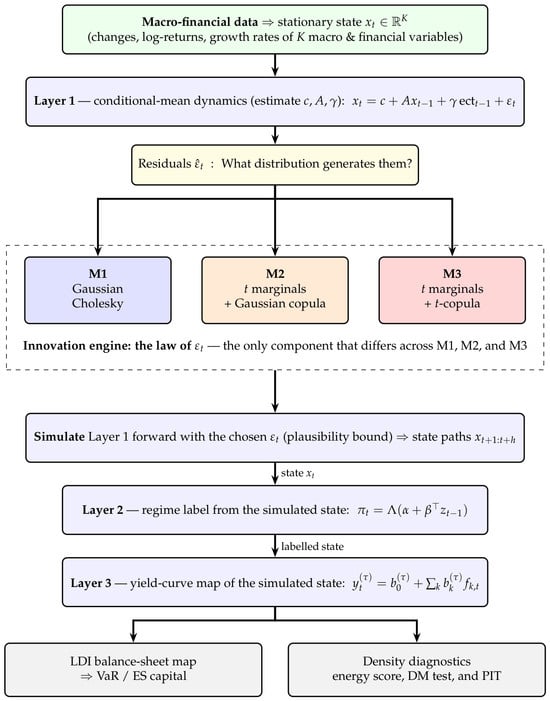
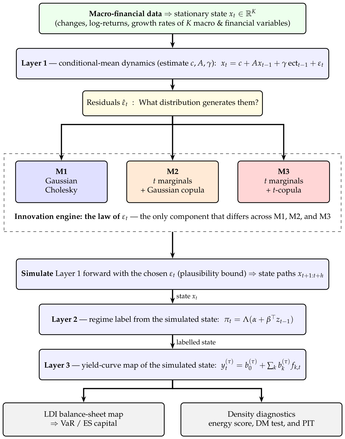
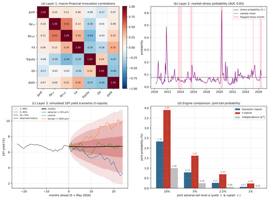
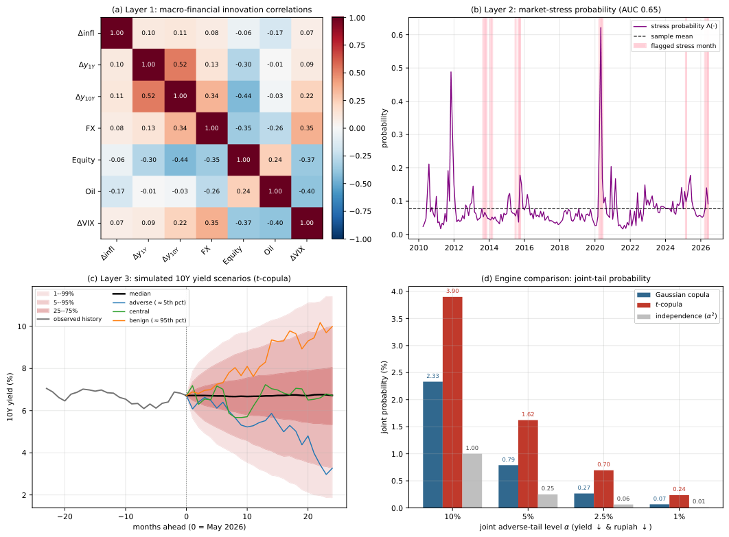
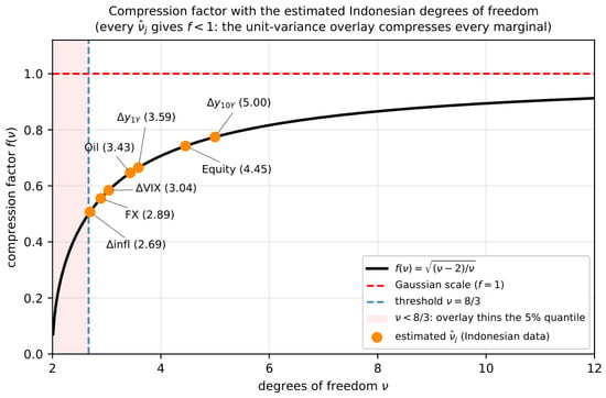
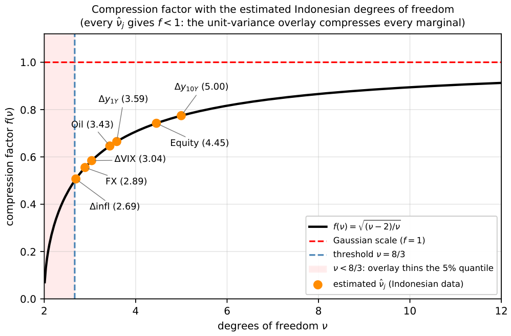
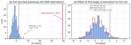
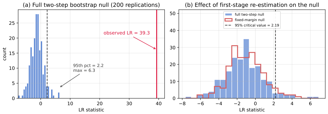
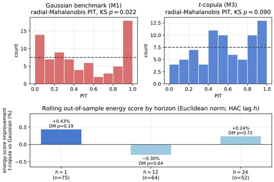
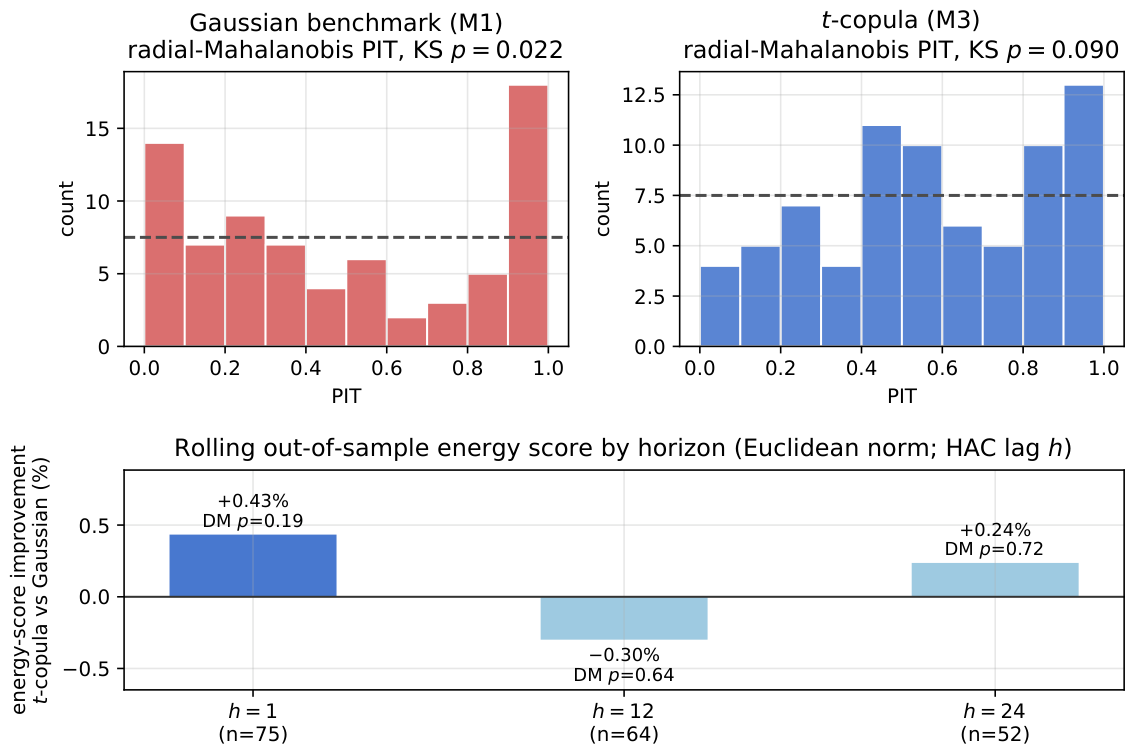
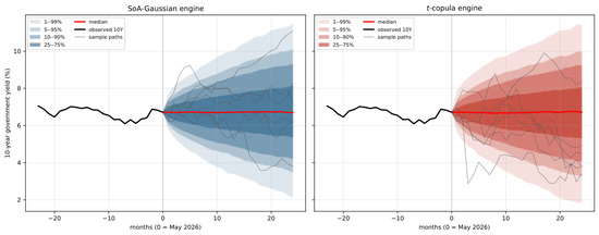
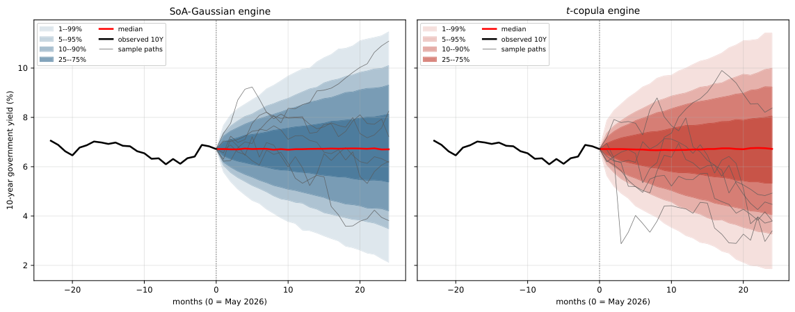
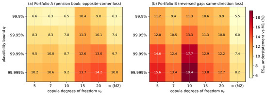
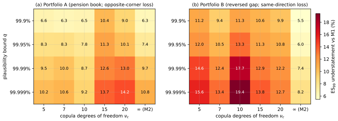
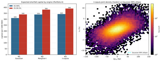
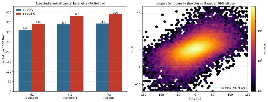
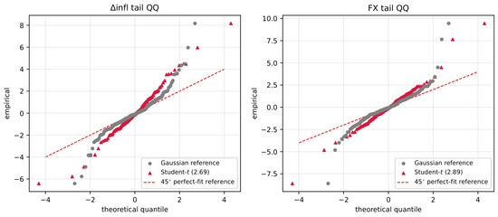
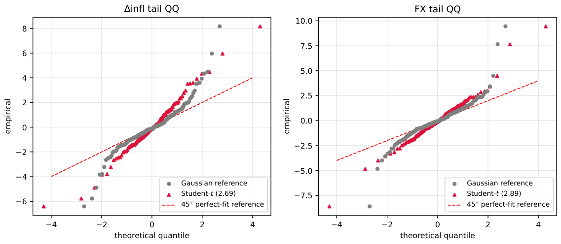

Disclaimer/Publisher’s Note: The statements, opinions and data contained in all publications are solely those of the individual author(s) and contributor(s) and not of MDPI and/or the editor(s). MDPI and/or the editor(s) disclaim responsibility for any injury to people or property resulting from any ideas, methods, instructions or products referred to in the content. |
© 2026 by the authors. Licensee MDPI, Basel, Switzerland. This article is an open access article distributed under the terms and conditions of the Creative Commons Attribution (CC BY) license.