


Highlights
What are the main findings?
- A causal filter strategy based on the NOTEARS-Linear-based Prediction Model (NLBPM) improved return-based performance by restricting trading to periods in which specific directed edges to the target were detected.
- NLBPM with a causal filter applied in the data period examined in this study outperformed both NLBPM without filtering and the benchmark LSTM in terms of monthly average return.
What are the implications of the main findings?
- Because NLBPM is interpretable, the causal structures inferred by the model can be used not only for prediction but also for designing trading strategies.
Abstract
In the highly volatile cryptocurrency market, trading decision support based on price prediction remains a challenging task. Although machine learning and deep learning techniques have been widely applied to cryptocurrency price prediction, many existing approaches rely on correlation-based black-box models, which limits interpretability and robustness. In this study, we employed a NOTEARS-Linear-based Prediction Model (NLBPM) that directly incorporated causal structures inferred through a causal discovery method as structural constraints within the prediction model. Unlike conventional approaches that focus primarily on minimizing prediction error, the NLBPM emphasized return maximization as its objective function, thereby prioritizing practical economic value. Using Bitcoin as a case study, we constructed a model to predict the direction of price movement four hours ahead and evaluated its performance using a rolling-window scheme with a one-month sliding window. Analysis of the inferred causal structures showed that the returns improved when trades were executed only during rolling-window trials in which specific directed edges to the target variable were detected. Based on this finding, we proposed a causal filter strategy that restricts trading to periods in which specific directed edges to the target variable are detected. In the data period analyzed in this study, the selected edge was the one from the opening price (Open) to the target variable. Backtesting experiments incorporating a transaction fee of 0.1% demonstrated that, while the benchmark LSTM model achieved a negative monthly average return of −3.20% and the NLBPM without filtering yielded −0.72%, the NLBPM with the Open filter attained a higher monthly average return of 10.35%. This study supports the usefulness of using inferred causal structure for cryptocurrency trading decision support.
1. Introduction
Since the advent of Bitcoin, cryptocurrencies built upon blockchain technology have rapidly evolved from decentralized means of value exchange into a major asset class in global financial markets [1]. However, cryptocurrency markets depend on a wide range of complex factors, including macroeconomic indicators, market sentiment, regulatory policies, and mining difficulty, and consequently exhibit extremely high price volatility compared with traditional financial assets [2,3,4]. While such characteristics offer investors opportunities for substantial returns, they also entail a high risk of severe capital losses. As a result, accurately and robustly predicting cryptocurrency price movements has become a critically important yet challenging problem in both academic research and financial practice.
A wide variety of approaches for cryptocurrency price prediction have been proposed to date, including statistical models, machine learning (ML), and deep learning (DL) techniques. Several comprehensive survey papers have systematically reviewed the effectiveness and limitations of these approaches. Early surveys [5] noted that statistical models suffer from limited predictive performance in cryptocurrency markets, due to their reliance on strong statistical assumptions and the lack of clearly observable seasonality. In contrast, machine learning techniques have been positioned as important predictive tools capable of learning complex relationships from market data. More recent surveys [6] have highlighted that, in addition to classical ML models, DL models such as recurrent neural networks (RNNs), Long Short-Term Memory (LSTM), gated recurrent units (GRUs), and deep reinforcement learning (DRL) are effective in handling nonlinearity and long-term dependencies, and may become core technologies in future research. These studies also report that integrating heterogeneous data sources—such as social media sentiment and macroeconomic indicators—can further improve predictive performance. Another comprehensive review [7] reports that although DL models often achieve high prediction accuracy, they are not universally superior, and hybrid deep learning architectures such as ConvLSTM, LSTM–GRU, and MRC–LSTM have emerged as mainstream approaches to overcome the limitations of single models. Furthermore, the development toward novel architectures, including Transformer-based models, has been identified as a promising research direction. Nevertheless, despite extensive research efforts, cryptocurrency price prediction remains highly complex, and important challenges regarding practical effectiveness in real-world trading applications remain unresolved.
With respect to statistical approaches, linear models such as the Autoregressive Integrated Moving Average (ARIMA) model [8,9] are effective in capturing short-term autocorrelation structures in the conditional mean of price series, while Generalized Autoregressive Conditional Heteroskedasticity (GARCH) models [10] have been widely employed to model volatility clustering through time-varying conditional variance. However, cryptocurrency markets are characterized by strong nonstationarity and abrupt price fluctuations, which often violate the linearity and distributional assumptions underlying these models, thereby limiting their adaptability to structural changes in market dynamics.
To overcome the limitations of statistical models, various ML-based models have been employed, including Support Vector Machines (SVMs) [11], Artificial Neural Networks (ANNs) [12], Random Forests (RFs) [13], XGBoost [14], and LightGBM [15], with several comparative studies evaluating these models [16,17]. These models are well suited for modeling nonlinear relationships and have demonstrated improved predictive accuracy compared with traditional statistical approaches. However, their performance heavily depends on feature engineering, leading to substantial variability in prediction accuracy. Moreover, a fundamental limitation of many machine learning models is their limited ability to handle large-scale sequential time series data, making it difficult to effectively learn long-term temporal dependencies.
DL-based models have thus been regarded as one of the most promising solutions to address these challenges. Among them, LSTM networks [18,19,20,21] and their variants, such as bidirectional LSTM (Bi-LSTM) and GRU [22,23], have been most frequently applied to cryptocurrency price prediction. The LSTM architecture is particularly well suited for capturing long-term dependencies in sequential data and has proven effective in modeling temporal patterns in financial time series. Unlike conventional machine learning models, LSTM networks naturally handle time-ordered data. Furthermore, techniques such as dropout and batch normalization are often employed to mitigate overfitting and improve generalization performance. Research on hybrid deep learning models extending LSTM has also progressed, and CNN–LSTM-based architectures, such as ConvLSTM [24,25], have been reported to achieve strong predictive performance.
More recently, Transformer-based models that leverage attention mechanisms have been proposed as alternatives to LSTM-based sequence modeling approaches [26,27,28]. While LSTM processes data sequentially, Transformers operate in a parallel manner and employ self-attention mechanisms to directly capture dependencies between distant elements within a sequence. This property improves computational efficiency and allows the model to capture abrupt changes in market sentiment and long-term trend shifts more rapidly. Although Transformer-based models are still under extensive empirical investigation, their ability to process multiple data points simultaneously has been shown to be particularly advantageous for high-frequency trading data and for integrating multimodal information, such as price series and textual data.
Despite these advances, three fundamental challenges remain in cryptocurrency price prediction using ML and DL models.
First, many existing methods rely primarily on correlations among variables, leading to an inherent overdependence on correlation-based prediction. Cryptocurrency markets are highly sensitive to regulatory changes and macroeconomic shocks, and thus exhibit multiple regimes whose statistical properties evolve over time [29,30]. Under such non-stationary environments, ML and DL models that learn correlations among numerous variables tend to overfit transient correlation structures and noise specific to the training period, resulting in degraded generalization performance. In fact, it has been reported that, in univariate cryptocurrency time series forecasting, complex ML and DL models do not consistently outperform simple naive models, and that their predictive performance deteriorates substantially when the parameters of the time window and forecast horizon change [31]. This observation is consistent with studies demonstrating that the predictive performance of DL models can theoretically degrade substantially in nonstationary time series where data distributions change over time [32]. These findings suggest that correlation-based prediction models face fundamental limitations in cryptocurrency markets characterized by nonstationarity and regime shifts. Given the limitations of correlation-based prediction, adopting a prediction framework based on a causal perspective can serve as one effective solution.
Second, ML and DL models suffer from low interpretability due to their model complexity. This issue is referred to as the black-box problem [33,34]. As a result, the difficulty in providing a clear basis for predictions may hinder the practical use of prediction models in financial practice, where accountability is required. Recent studies have applied Shapley Additive Explanations (SHAP)—an Explainable AI (XAI) method—to cryptocurrency price forecasting. Specifically, SHAP has been used to post hoc explain the features contributing to predictions in hybrid CNN–LSTM models [35]. However, as long as prediction models are trained based on correlations, there remains a risk that they learn spurious correlations; in such cases, even the application of XAI methods may lead to misleading explanations. Therefore, rather than explaining prediction outcomes post hoc, learning causal information as the internal structure of prediction models can serve as one potential solution for providing reliable explanations.
To address the limitations of correlation-based models and the black-box problem, a limited number of studies have recently reported methods that utilize causal information in cryptocurrency markets. Unlike correlations, causal relationships are relatively stable under changing market environments, and thus have been pointed out as being useful for robust and interpretable prediction [36]. Luo et al. [36] incorporated a causality matrix estimated from time-series data into a Graph Neural Network as a graph structure and applied it to Bitcoin price prediction. Their approach reported improved predictive performance by augmenting correlation-based graph representations with indicators of causal influence derived from temporal dependencies. However, while a causality matrix is useful as a quantitative measure of influence among variables, it differs from structural equation-based causal models that explicitly assume causal directionality and acyclicity. Amirzadeh et al. [37] constructed a network of causal dependencies among variables using Dynamic Bayesian Networks (DBNs), which are state transition models, and performed directional prediction of price movements based on probabilistic transitions.
Because DBNs represent conditional dependencies among variables using directed acyclic graphs (DAGs), they possess a certain degree of causal interpretability. Nevertheless, the edges in DBNs represent influence relationships conditioned on temporal transitions and latent states, rather than explicitly assuming causal effects as structural equations that describe the data-generating process. As a result, it is not necessarily straightforward to intuitively interpret the magnitude of each variable’s causal impact on prediction outcomes in the form of path coefficients. On the other hand, when broadening the scope to financial forecasting including stock markets, some studies have utilized causal discovery methods for feature selection [38] and feature engineering [39] with the aim of identifying intrinsically important variables prior to incorporating them into prediction models. From the above survey, prediction models incorporating causal information in the cryptocurrency market are still in their early stages, leaving considerable room for further research.
Third, in current cryptocurrency price prediction research, there is a practical issue that improvements in the statistical predictive performance do not necessarily translate into securing trading profitability. Otabek and Choi [6], through a systematic review of prior studies, pointed out that improvements in prediction error and classification performance do not necessarily lead to improved trading profitability. Shintate and Pichl [40] reported that, in trend prediction classification for high-frequency Bitcoin time series using DL models, their model achieved high performance in terms of F1-score; however, when the predicted outcomes were applied as a simple trading rule based on up/down/static signals, returns during the test period did not outperform a Buy-and-Hold strategy. This provides an example showing that improving predictive performance does not necessarily directly lead to improved trading profitability. One underlying reason for this gap is the fundamental inconsistency between error minimization as the optimization objective during model training and profit maximization as the trader’s objective. Therefore, to construct cryptocurrency prediction models that are suitable for financial practice, a key challenge lies in whether profit maximization can be incorporated as an explicit optimization objective from the training stage.
In this study, to overcome the limitations of existing cryptocurrency price prediction models, we employed a prediction model that directly incorporated causal structures inferred through a causal discovery method as structural constraints. This model performed predictions based on causal paths, thereby ensuring high interpretability and enabling causal explanations of market mechanisms underlying price movements. Furthermore, in optimizing the prediction model, we departed from the conventional objective of minimizing prediction error and instead emphasized return maximization as the objective function. In addition, this study proposed a trading strategy by analyzing characteristics of the inferred causal structure. Through this study, we demonstrate the effectiveness of the proposed strategy as a trading decision support method that aims to simultaneously achieve high interpretability and high returns, an aspect that has not been sufficiently examined in prior studies.
2. Materials and Methods
2.1. Data
In this study, Bitcoin (BTC), the most representative cryptocurrency with the largest market size and liquidity, was selected as the target asset. The price data consisted of BTC/USDT 4-h candlestick data (six observations per day) obtained from the Binance cryptocurrency exchange, covering the period from March 2018 to September 2025.
Financial price prediction generally employs both fundamental indicators, which are based on corporate financial conditions and macroeconomic trends, and technical indicators, which are derived by applying mathematical transformations to historical market data. In this study, only technical indicators were used. This is because fundamental indicators often include irregularly updated information and qualitative components, making them difficult to apply to prediction models that require regular, time-aligned inputs. In contrast, technical indicators are quantitative and regularly updated time-series data; therefore, they are suitable for constructing sequential prediction models. The features used in the prediction model included basic price information and major technical indicators. Because such price information and technical indicators are relatively easy for general investors to obtain, they are also suitable for examining a prediction framework based on widely accessible market data.
The target variable was defined as a binary variable representing the direction of price movement at the next time step (four hours ahead). Specifically, an upward movement in the closing price relative to the current closing price was labeled as 1, whereas a downward movement or no change was labeled as 0.
A total of 20 features were prepared for predicting the target variables: five price-related variables (Open, High, Low, Close, and Volume) and 15 technical indicators, as listed in Table 1. The technical indicators were classified into four categories: trend indicators, oscillator indicators, volatility indicators, and momentum indicators.
Table 1.
Features used to predict the direction of price movements.
2.2. Causal-Structure-Based Prediction Model
2.2.1. Architecture of the Prediction Model (NLBPM)
In this study, a prediction model was constructed to predict the direction of price movement at time (four hours ahead) based on basic price information and technical indicators at time . The prediction model was implemented using the DAGClassifier class provided by the CausalNex library [41], which integrates causal discovery with a classification task and is therefore well suited for predictions based on causal structures. For causal discovery within DAGClassifier, the NOTEARS algorithm (Non-combinatorial Optimization via Trace Exponential and Augmented Lagrangian for Structure Learning) [42] is employed. The prediction model learns a directed acyclic graph (DAG), in which dependencies among variables are represented by directed edges with no cyclic paths. In causal discovery, acyclicity is a crucial requirement that prevents contradictory structures, such as cases where variable A causes B while B simultaneously causes A. Although DAGClassifier is originally designed to employ nonlinear models based on multilayer perceptrons (MLPs), this study adopted a linear causal model, namely NOTEARS-Linear, by configuring the DAGClassifier class without hidden layers, to reduce computational cost and improve interpretability. The resulting model is referred to as the NOTEARS-Linear-based Prediction Model (NLBPM). While financial time series exhibit strong autocorrelation, this study explicitly defines a temporal structure by predicting the target variable at time from features at time , thereby avoiding contemporaneous ambiguity. Although NOTEARS assumes i.i.d. data, this formulation alleviates potential violations by enforcing a strict temporal ordering between inputs and the target variable. Importantly, in this study, NOTEARS is employed as a structural constraint within a prediction model rather than purely for causal discovery, which distinguishes this approach from standard causal discovery settings and aligns it with common practices in ML-based financial forecasting where lagged features are routinely utilized.
It should be acknowledged, however, that enforcing temporal ordering addresses contemporaneous ambiguity but does not fully resolve the non-i.i.d. nature of the samples used for DAG structure estimation, as financial time series exhibit autocorrelation and volatility clustering that persist across observations. In this study, two practical measures are adopted to mitigate this concern. First, the rolling-window scheme with a fixed 15-month training window provides a local stationarity approximation: by re-estimating the DAG structure independently in each RW trial, the model adapts to evolving market conditions rather than relying on a single structure estimated over the full sample period. Second, L1 regularization applied to the weighted adjacency matrix promotes sparse edge selection, reducing the risk of overfitting to transient autocorrelation patterns specific to the training window. Nevertheless, we recognize that time-series-specific causal discovery methods, such as DYNOTEARS [43], would be more theoretically appropriate for handling autocorrelated observations. However, these methods produce causal graphs with explicit lag terms, where multiple directed edges are estimated for each variable across different time lags. While this richer temporal structure may better capture the dynamics of financial time series, it also increases the complexity of the causal filter design, as the filter condition must be defined over combinations of lagged edges rather than a single directed edge. Given that interpretability and simplicity of the causal filter are central to the trading strategy proposed in this study, we adopt NOTEARS-Linear as a practical compromise that provides directly interpretable edge weights at a single time lag. Exploring time-series-specific causal discovery methods and their implications for causal filter design remains an important direction for future work.
Figure 1 shows a schematic illustration of the architecture of NLBPM. The input layer consists of variables, including features at time and a binary target variable representing the direction of price movement at time . The notation denotes the value of feature for sample , and denotes the corresponding target value. To stabilize training, continuous variables were standardized to have zero mean and unit variance.
Figure 1.
Schematic illustration of the architecture of NLBPM.
The reconstruction layer reconstructs the input data using an estimated weighted adjacency matrix and a node-wise bias vector . A structural constraint (Tabu constraint) was imposed to ensure that the target variable remained a leaf node, explicitly prohibiting edges directed from the target variable to features. This constraint concentrates gradient signals on causal inflows into the target variable (i.e., contributions to the prediction), resulting in edge weights in that reflect the importance of each feature with respect to the target variable. Although the prediction model shares a similar formulation with linear structural equation models (SEMs), it differs from conventional SEMs in that DAG constraints ensuring acyclicity are directly incorporated and edge weights are estimated through continuous optimization.
During the inference phase, the learned is used for data reconstruction while treating the target variable as unobserved (i.e., without using observed target values). For sample , the reconstructed target value is computed as
where denotes the edge weight from feature to the target variable. The predicted probability of an upward price movement is then given by through the sigmoid function . Finally, a binary decision on the direction of price movement is output by applying a threshold of 0.5 to , where 1 indicates an upward movement, and 0 indicates a downward movement.
2.2.2. DAG Discovery Using NOTEARS
Traditionally, DAG discovery has been treated as a combinatorial optimization problem. Representative methods such as the PC algorithm and Fast Causal Inference (FCI) search for graph structures by repeatedly conducting conditional independence tests among variables; however, these approaches suffer from severe scalability issues, as the computational cost increases exponentially with the number of variables. In contrast, NOTEARS [42] is a groundbreaking method in the field of causal discovery that formulates DAG learning as a continuous optimization problem.
In NOTEARS, acyclicity is imposed on the weighted adjacency matrix by defining a continuously differentiable constraint function as follows:
Here, denotes the trace of a matrix, denotes the Hadamard product, represents the matrix exponential, and is the number of variables (including the target variable and the features ). This function mathematically represents the total number of directed paths in the graph, and the condition constitutes a necessary and sufficient condition for the extracted structure to be a strict DAG. This formulation enables efficient DAG discovery using gradient-based optimization methods.
For practical implementation, NOTEARS adopts an approximation of the acyclicity constraint using a matrix polynomial to improve computational efficiency. Specifically, the constraint function is approximated as follows:
where denotes the identity matrix.
2.2.3. Objective Function and Optimization of NLBPM
In the NLBPM, the learning process is formulated as a continuous optimization problem with an equality constraint to simultaneously achieve causal structure estimation and predictive performance optimization. Let denote the feature matrix, denote the binary target vector, denote the weighted adjacency matrix, and denote the node-wise bias vector. Under this setting, the optimization problem is defined as
The first and second terms respectively represent the data-fitting loss and an L1 regularization term, where denotes the regularization coefficient. To suppress overfitting and promote sparse edge selection, L1 regularization is applied to .
As the data-fitting loss, a squared reconstruction loss is applied to the continuous feature variables, which consist of price information and technical indicators, while binary cross-entropy (LogLoss) is applied to the binary target variable representing the direction of price movement. The loss function is defined as
The first and second terms respectively represent the reconstruction error of the full feature matrix and the classification error of the target variable. Here, denotes the squared Frobenius norm, and denotes the reconstructed feature matrix. The predicted value of the target variable is converted into a probability through the sigmoid function when computing the LogLoss.
To solve this equality-constrained optimization problem, the Augmented Lagrangian Method is employed. The constrained problem is transformed into the unconstrained objective:
where the third and fourth terms correspond to the DAG constraint. The penalty parameter and the Lagrange multiplier are automatically updated during training. At each iteration, is dynamically increased based on the convergence behavior of the acyclicity constraint , while is cumulatively updated according to the constraint residual. This procedure accelerates convergence toward acyclicity while maintaining predictive performance, thereby ensuring convergence to a DAG structure. The minimization of is performed using the L-BFGS-B algorithm, a quasi-Newton method suitable for differentiable optimization.
2.3. Model Optimization and Performance Evaluation Using Walk-Forward Analysis
2.3.1. Design of the Rolling-Window Scheme
In this study, to adapt to changes in the cryptocurrency market environment and to evaluate the robustness of the prediction model, a walk-forward analysis based on a rolling-window (RW) scheme was adopted. As illustrated in Figure 2, RW trials were performed by sliding the entire window forward by one month at each iteration. A total of 48 RW trials were conducted over a four-year period. These 48 RW trials were used for internal comparison and for selecting strategy settings, including the fixed-length training window, during the exploratory phase of trading strategy design. Therefore, these results should be interpreted not as the final confirmatory evaluation of the proposed method, but as an exploratory procedure. The final evaluation of the prediction model and trading strategy was conducted in the backtesting experiment described later.
Figure 2.
Schematic illustration of the rolling-window scheme.
In each RW trial, Step A (Hyperparameter Optimization) was first executed, followed by Step B (Performance Evaluation), as described below. The test period spanned from October 2020 to September 2024, with each RW trial using a one-month test interval. The validation period consisted of the one-month interval immediately preceding the test interval. For the training period, a fixed-length window scheme was introduced. The training period was defined as a fixed-length window ending two months prior to the test interval, and the window length was varied from 12 to 30 months in three-month increments (12, 15, 18, 21, 24, 27, and 30 months), resulting in seven window configurations.
- Step A: Hyperparameter Optimization
In Step A, the NLBPM was trained using data from the training window. During the subsequent one-month validation interval, trading simulations were conducted according to the trading rules described later, based on four-hour-ahead price direction prediction signals. The hyperparameter optimized in this step was the L1 regularization coefficient . The hyperparameter search was performed through iterative trials using the Bayesian optimization framework Optuna [44]. As the search algorithm in Optuna, the Tree-structured Parzen Estimator (TPE) was employed. TPE probabilistically estimates promising regions of the parameter space based on the outcomes of previous trials, enabling efficient exploration.
A key characteristic of this study is the direct maximization of return-based performance such as the monthly average return described below, rather than conventional metrics such as classification performance. Figure 3 illustrates a schematic overview of the NLBPM optimization process. Optuna repeatedly executed a cycle consisting of DAG structure learning, price direction prediction, and return calculation. By feeding back the resulting returns, Optuna estimated values expected to yield higher returns and identified the corresponding optimal weighted adjacency matrix . Finally, a return-maximizing model was obtained.
Figure 3.
Schematic illustration of the NLBPM optimization process.
- Step B: Performance Evaluation
In Step B, the optimal value of identified in Step A was fixed, and the NLBPM was retrained accordingly. To reflect recent market dynamics, the validation interval used in Step A was incorporated into the retraining data. The retrained model was then evaluated over the one-month test interval using trading simulations based on the predefined trading rules.
2.3.2. Trading Rules
The trading rules adopted in this study execute trades mechanically according to the flow illustrated in Figure 4, based on the price direction predicted by the NLBPM. Specifically, trading decisions are made according to the conditions described below, depending on the current Bitcoin position state (no position or holding a position).
Figure 4.
Trading decision flow based on price direction prediction.
When no position is held, a buy order is executed if an upward signal is predicted, in order to capture potential price increases. Conversely, if a downward signal is predicted, no trade is executed, and the no-position state is maintained to avoid downside risk. When a position is held, no trade is executed if an upward signal is predicted, and the existing position is maintained without additional purchases, assuming that the price increase will continue. If a downward signal is predicted, a sell order is executed, and the entire position is immediately liquidated to realize profits or limit losses. Under these trading rules, the strategy always selects either full investment (full buy) or full liquidation (full sell); position scaling and partial liquidation are not permitted. This constitutes a long-only strategy, as the model can only take buy positions and does not engage in short-selling.
The trading capital was reset to a fixed amount at the beginning of each RW trial. This capital reset was adopted to compare RW trials under the same initial conditions and to statistically evaluate the effectiveness of the monthly returns generated by the prediction model and trading strategy. Because cumulative performance is strongly dependent on a single realized path, this study placed greater emphasis on standardized month-level evaluation than on cumulative path-based evaluation.
Trading simulations were conducted under fee-adjusted trading conditions that incorporated transaction fees for both buy and sell transactions. Specifically, according to the transaction fee table of Binance [45], four levels of one-way transaction fees—0.00% (no fee), 0.06%, 0.08%, and 0.10%—were considered to examine the impact of transaction costs on returns.
In this study, the analysis focused on prediction using price information and technical indicators that are relatively easy for general investors to obtain. Because modeling other execution-related costs, such as slippage, bid–ask spread, and market impact, requires more detailed market microstructure information beyond such data, these factors were not incorporated into the present trading simulation. The reported returns are based on simplified trading assumptions and may therefore be optimistic compared to real trading conditions; however, this does not imply that they are meaningless for supporting decision-making. In cryptocurrency price prediction studies based primarily on OHLCV (Open, High, Low, Close, and Volume) data, it is difficult to fully replicate real trading conditions, which remains a common challenge in this research field. It should also be noted that, for highly liquid trading pairs such as BTC/USDT on major exchanges, the typical bid–ask spread for retail-sized orders corresponds to a slippage considerably lower than the transaction fees applied in this study. The transaction fee of 0.10% adopted in this study therefore already substantially exceeds the combined cost of the exchange fee and realistic slippage, serving as a conservative estimate of execution costs.
2.3.3. Evaluation Metrics for Predictive Performance
In this study, return-based metrics were adopted as the primary evaluation criteria for predictive performance, as they provide an economically meaningful criterion for decision-making, rather than conventional statistical classification metrics. In addition, classification metrics were used as secondary evaluation criteria. This evaluation framework enabled a comprehensive assessment of predictive performance.
Return-based metrics were computed based on the trading results obtained from all RW trials. The return-based metrics used in this study were the monthly average return and win rate.
Let denote the return obtained in RW trial . The monthly average return is defined as:
In this study, returns are aggregated arithmetically across RW trials because each RW trial is treated as an independent evaluation period with a fixed initial capital. Therefore, the monthly average return represents the average performance across independent trials rather than compounded portfolio growth over time.
To evaluate the frequency of positive returns, an indicator variable is defined for each RW trial as follows:
Using this indicator, the win rate is then calculated as:
Classification metrics were derived from the confusion matrix, which consists of True Positive (TP), True Negative (TN), False Positive (FP), and False Negative (FN) components. Based on these components, Accuracy, Precision, Recall, and F1-score were computed. Accuracy represents the proportion of correctly predicted upward and downward movements. Precision measures the proportion of actual upward movements among those predicted as upward, while Recall indicates the proportion of correctly predicted upward movements among all actual upward movements. The F1-score is defined as the harmonic mean of Precision and Recall.
Each classification metric was computed for each RW trial . Let denote a classification metric obtained in RW trial ; the monthly average classification performance is then calculated as:
2.4. Trading Strategy Based on Characteristic Directed Edges in the Inferred Causal Structure
In this study, in contrast to a baseline trading strategy that uniformly executes trades according to predefined trading rules whenever prediction signals are generated, a causal filter strategy based on the causal structures inferred by the NLBPM was proposed to improve returns.
Under the causal filter strategy, trading was conducted only for RW trials in which specific directed edges to target variables were detected in the inferred causal structures. The specific directed edges used as filters were determined in advance during the exploratory phase for trading strategy design, prior to backtesting experiments. To evaluate the effectiveness of the proposed causal filter strategy, return-based performance was compared between scenarios with and without the application of the causal filter.
The candidate filters were defined by all directed edges from individual features to the target variable, and their return-based performance across the exploratory phase RW trials was fully evaluated and reported to ensure transparency of the selection process. Candidate filters were assessed based on win rate, the number of active RW trials, and consistency of return improvement over the no-filter baseline. The selected filter was fixed prior to the backtesting experiment and was not modified based on backtesting outcomes.
It should be emphasized that the causal filter is not an externally imposed market-timing rule but an intrinsic output of the NLBPM framework. Specifically, the filter activates solely based on whether a directed edge to the target variable is detected in the causal graph estimated by NLBPM during each RW trial; it is therefore inseparable from the causal discovery process itself. Because the benchmark model LSTM does not perform causal structure estimation, it is fundamentally incapable of generating an equivalent filter. Accordingly, the comparison between NLBPM with the causal filter and LSTM represents a comparison of two complete and self-contained trading systems with inherently different capabilities, which is the intended scope of evaluation in this study.
2.5. Benchmark Model
To comparatively evaluate the effectiveness of the proposed NLBPM, a deep learning model, namely, LSTM, was adopted as a benchmark. LSTM is a type of recurrent neural network (RNN) that is well suited for learning long-term dependencies in time-series data. By introducing a memory cell together with three gating mechanisms—the forget gate, input gate, and output gate—LSTM is able to retain long-term temporal information.
LSTM has been widely used in cryptocurrency price prediction. However, due to its strong nonlinearity and complex internal structure, LSTM suffers from the black-box problem, making it difficult to interpret the rationale behind its predictions. In this respect, LSTM fundamentally differs from the NLBPM, which is designed as an interpretable prediction model based on causal structures.
The hyperparameter settings of the LSTM used in this study were based on those reported in a related study [46]. In particular, the input sequence length (timesteps), which affects predictive performance and determines how far back past observations are referenced at prediction time, was explored in this study. Within the same rolling-window scheme used for the NLBPM, several timesteps—6 (1 day), 18 (3 days), 30 (5 days), and 42 (7 days)—were evaluated, and the timesteps value that maximized returns was selected.
In addition to LSTM, a Buy-and-Hold strategy was employed as a market benchmark to assess whether the returns of the proposed strategy exceed those obtainable from the overall market movement. Under the Buy-and-Hold strategy, Bitcoin was purchased at the beginning of each one-month test interval and held until the end of the interval, following the same rolling-window evaluation framework used for the other models.
2.6. Design of the Backtesting Experiment
In this study, a backtesting experiment was conducted to examine whether the proposed causal filter strategy remained effective when applied to future unseen data. With the causal filter strategy fixed, the same rolling-window scheme as that used in the exploratory phase for trading strategy design, incorporating training, validation, and test intervals, was applied to evaluate trading performance. The overall test interval used in the backtesting experiment covered one year from October 2024 to September 2025 (12 months in total), and this period was completely excluded from the exploratory phase for trading strategy design. Because return-based optimization may be sensitive to validation-period market regimes, this fully excluded 12-month period was used as an additional robustness check.
3. Results
3.1. Return-Based Performance of NLBPM
The predictive performance of financial market models is highly dependent on the length of the data period used for training. If the training period is too short, the model may fail to capture sufficient market patterns; conversely, if it is too long, outdated information that deviates from recent market structures may be incorporated, potentially leading to a degradation in predictive performance. To identify an appropriate fixed-length training window for the NLBPM, this study compared seven fixed-length windows at three-month intervals: 12, 15, 18, 21, 24, 27, and 30 months.
For each fixed-length window, 48 rolling-window (RW) trials were conducted by sliding the window forward in one-month increments. In each RW trial, returns were computed by executing the trading rules defined in this study. Predictive performance was evaluated using return-based metrics as the primary criteria and classification metrics as secondary criteria. In addition, to approximate trading conditions, four levels of one-way transaction fees—0.00% (no fee), 0.06%, 0.08%, and 0.10%—were applied based on the transaction fee table of Binance [45].
Table 2 presents the return-based performance of NLBPM across different fixed-length windows. The evaluation metrics include the monthly average return, win rate, and monthly average number of trades under each transaction fee rate. In addition, Figure 5 visualizes the impact of transaction fee variations on the monthly average return. The results indicated that, regardless of the transaction fee level, the highest monthly average return was achieved when a window length of 15 months was employed. In particular, under a commonly applied transaction fee of 0.10%, only the 12-month window and the 15-month window maintained positive monthly average returns. In contrast, all window lengths of 18 months or longer yielded negative returns, with the lowest value observed for the 27-month window. These findings demonstrate that the choice of training window length has an important impact on trading performance.
Table 2.
Return-based performance of NLBPM across different fixed-length windows.
Figure 5.
Monthly average returns of NLBPM under different transaction fee rates across different fixed-length windows.
Focusing on the win rate, the 12-month window achieved the highest value at 50.00%, exceeding those of the 15-month window and the 21-month window. However, the 15-month window records the highest monthly average return, suggesting that a higher win rate does not necessarily translate into greater overall returns. This result implies that, although the 15-month window has a lower win rate than the 12-month window, it may better capture a trade pattern characterized by larger gains per trade or more effectively controlled losses. Since the primary objective of this study is return maximization, particular emphasis is placed on the monthly average return as the main performance indicator.
An examination of the monthly average number of trades executed based on the prediction signals revealed a clear increasing trend in trading frequency as the fixed-length window becomes longer, rising from 19.67 trades for the 12-month window to 26.52 trades for the 30-month window. Under the trading rules adopted in this study, no new trade is executed as long as the prediction signal continues in the same direction. Therefore, an increase in the number of trades indicates more frequent reversals of prediction signals. When a shorter fixed-length window is used, prediction signals tend to persist in a single direction for longer periods. In contrast, longer fixed-length windows appear to react more sensitively to minor market fluctuations, leading to more frequent switches between upward and downward predictions. Consequently, an increase in the monthly average number of trades is considered to lead to the accumulation of transaction fees, thereby reducing the monthly average returns. Indeed, for longer fixed-length windows (the 27-month and 30-month settings), the difference in monthly average return between the 0% and the 0.10% transaction fee conditions exceeded 5%. By contrast, under the 15-month window, where the monthly average number of trades remains relatively restrained, the corresponding reduction in return was limited to approximately 4%. These findings indicate that the 15-month window demonstrates superior resilience to transaction costs. Based on these results, the 15-month fixed-length window, which exhibited the highest returns even after accounting for transaction costs, was selected as the most promising window length in the exploratory phase for trading strategy design and was adopted in the subsequent backtesting experiment.
3.2. Price Direction Classification Performance of NLBPM
Table 3 presents the price direction classification performance of NLBPM across different fixed-length windows. The evaluation metrics include the monthly average Accuracy, Precision, Recall, and F1-score computed over 48 RW trials. The results showed that the monthly average Accuracy remained relatively stable across fixed-window length settings, ranging from 52.6% to 52.8%. In contrast, notable differences were observed in the monthly average Precision and Recall depending on the fixed-window length. The highest Precision value of 0.566 was achieved with the 12-month and 21-month windows, whereas it decreased to 0.540 for the 24-month window, corresponding to a difference of 0.026. Furthermore, the monthly average Recall and F1-score exhibited a decreasing trend from the 15-month to the 24-month window, followed by a recovery for longer windows. The 30-month window achieved the highest monthly average F1-score of 0.527 across all settings. These results indicate that classification metrics vary in a non-monotonic manner with respect to the length of the training window.
Table 3.
Price direction classification performance of NLBPM across different fixed-length windows.
A comparison of the classification performance with the return-based performance shown in Table 2 revealed that higher classification performance does not necessarily translate into higher returns. For example, although the 30-month window achieved the highest F1-score, it recorded a large negative monthly average return under the transaction fee of 0.1%. This discrepancy can be attributed to several factors. First, conventional classification metrics treat prediction errors equally. Second, under the long-only trading strategy adopted in this study, false positive predictions generate actual trading losses, whereas false negative predictions only result in missed opportunities. Furthermore, classification metrics do not account for the magnitude of price movements or whether the realized return exceeds transaction costs. In real financial trading, correct predictions during large price movements and the ability to secure return margins exceeding transaction costs play a decisive role in determining overall profitability.
3.3. Causal Structures Inferred by NLBPM
The causal structures inferred in all 48 RW trials under the 15-month fixed-length window setting were analyzed to detect the direct causes (parent nodes) of the target variable. The frequency with which directed edges from each feature to the target variable were detected is reported in Supplementary Material S1. Notably, RSI_7 (7-period Relative Strength Index) was detected as a parent node of the target variable in 46 out of 48 trials (95.8%), demonstrating an exceptionally high occurrence rate. This finding suggests that NLBPM robustly captures the influence of oscillator-based indicators reflecting market overbought and oversold conditions. In contrast, the appearance frequencies of parent nodes other than RSI exhibit considerable variability.
Figure 6 illustrates the causal graphs corresponding to the top four RW trials that achieved the highest monthly average returns (1st: 27.28%, 2nd: 22.96%, 3rd: 19.65%, 4th: 18.97%). These high-performing graphs share commonalities. A notable common characteristic is the differentiated role of RSI depending on its period length. In all four cases, the short-term RSI_7 consistently exhibited a negative weight to the target variable, whereas the medium-term RSI_14 consistently showed a positive weight. Another notable finding was that the Open (opening price) appeared as a parent node of the target variable in all four high-return trials. This result suggests that restricting trading to RW trials in which a directed edge from the Open to the target variable is present is effective for achieving high monthly returns. The Open filter was therefore selected based on the following criteria evaluated during the exploratory phase: (1) It achieved the highest win rate (59.26%) among candidate filters with a sufficient number of active trading RW trials. (2) It was active in 27 out of 48 RW trials, providing substantially greater statistical reliability than filters active in only a small number of trials—for instance, the EMA_200 filter recorded a higher monthly average return (5.01%) but was active in only 2 trials, making its result potentially dependent on specific market conditions. (3) It showed consistent return improvement over the no-filter baseline. All candidate filter results are fully reported in Supplementary Material S1, ensuring transparency of the selection process. The selected filter was fixed prior to the backtesting experiment and was not modified based on backtesting outcomes.
Figure 6.
Causal graphs for the top four RW trials that achieved the highest monthly average returns. The red node indicates the target variable. Green and red values represent positive and negative weights. Thick edges denote the directed edges between the target variable and its parent nodes.
3.4. Trading Strategy Based on Inferred Causal Structure
Among the 48 RW trials, there are periods in which achieving positive returns is difficult. Avoiding trading during such periods can serve as an effective means of improving returns. Therefore, this study proposes a trading strategy that decides whether to execute trades for each RW trial based on insights obtained from the causal structures inferred by NLBPM. In this study, we define a causal filter strategy as an approach that restricts trading to RW trials in which specific causal relationships (directed edges) are detected. The return-based performance obtained by applying various causal filters, defined by directed edges from individual features to the target variable, is reported in Supplementary Material S1. Among these filters, executing trades only in RW trials in which a directed edge from the Open (opening price) to the target variable existed demonstrated high and consistent returns. This condition is referred to as the Open filter.
Table 4 compares the return-based performance of NLBPM without filtering, NLBPM with the Open filter, and LSTM under a fixed-length window of 15 months, a transaction fee rate of 0.1%, and the trading rules adopted in this study, based on 48 RW trials. For the LSTM, multiple input sequence lengths (timesteps) were evaluated (see Supplementary Material S2), and the results with timesteps set to 18 (three days), which achieved the highest performance, are shown. As a result, NLBPM without filtering achieved a win rate of 41.67% and a monthly average return of 0.36%. NLBPM with the Open filter achieved a win rate of 59.26% and a monthly average return of 3.34%. On the other hand, LSTM recorded the lowest values for both return-based metrics, with a win rate of 33.33% and a negative monthly average return of −2.86%. However, the Open filter should be interpreted as the best-performing filter in the present exploratory phase for trading strategy design, rather than as a universally optimal filter.
Table 4.
Return-based performance of prediction models under a 0.1% transaction fee.
Table 5 compares the price direction classification performance of prediction models under the same conditions. For NLBPM without filtering, the monthly average Accuracy, Precision, Recall, and F1-score were 0.526, 0.561, 0.581, and 0.521, respectively. When the Open filter was applied, these values became 0.527, 0.576, 0.579, and 0.524. The application of the Open filter led to improvements in all classification metrics except recall. On the other hand, LSTM exhibited lower classification performance than both NLBPM without filtering and NLBPM with the Open filter across all metrics.
Table 5.
Price direction classification performance of prediction models.
3.5. Backtesting Experiment
In the backtesting experiment, the one-year period immediately following the exploratory phase for trading strategy design was treated as a completely unseen test period. A total of 12 RW trials were conducted to examine the effectiveness of the causal filter strategy, using the Open filter selected in the exploratory phase for trading strategy design. In each RW trial, a one-month validation interval for hyperparameter optimization and a one-month test interval for performance evaluation were applied, following the same framework as in the exploratory phase for trading strategy design. The hyperparameters determined in the exploratory phase for trading strategy design were fixed throughout the backtesting experiment, with a fixed window length of 15 months for NLBPM and a timestep set to 18 for the LSTM model.
Table 6 presents the return-based performance of NLBPM without filtering, NLBPM with the Open filter, and LSTM under a transaction fee rate of 0.1%. When the Open filter was applied, trades were executed in four RW trials, no losing RW trials were observed, and the monthly average return reached 10.35%, indicating favorable performance. In contrast, both NLBPM without a filter and LSTM recorded win rates of only 41.67%, and their monthly average returns were negative.
Table 6.
Return-based performance of prediction models under a 0.1% transaction fee in the backtesting experiment.
To examine whether the returns of the proposed strategy exceed those obtainable from the overall market trend, a Buy-and-Hold benchmark was additionally evaluated under the same rolling-window framework, in which Bitcoin was purchased at the beginning of each one-month test interval and sold at the end. As shown in Table 6, the Buy-and-Hold benchmark achieved a monthly average return of 5.57% with a win rate of 66.67%, indicating that the backtesting period included both bullish and bearish months. Over the same period, NLBPM (Open Filter) achieved a monthly average return of 10.35%, exceeding the Buy-and-Hold benchmark. This suggests that the returns of the proposed strategy are not merely attributable to the overall upward market trend during the backtesting period. In contrast, both NLBPM (No Filter) and LSTM underperformed the Buy-and-Hold benchmark, indicating that the causal filter strategy, rather than the prediction model alone, was the key contributor to outperforming the market benchmark.
The Open filter was active in only four of the 12 RW trials, reflecting the sparse-trading nature of the strategy. The number of RW trials in which the Open filter is active also depends on the market conditions under which the corresponding directed edge is detected, and therefore does not simply increase with a longer test period. Accordingly, the reported win rate of 100% indicates that all four RW trials in which the filter was active had positive returns. The causal filter strategy is an event-driven approach in which trades are executed only when specific causal structures are detected. As a result, the number of trading instances is not determined by the length of the evaluation period, but by the frequency with which the corresponding causal conditions are satisfied. Therefore, even over a longer period, the number of trading instances may remain limited. In this sense, the reported results reflect the behavior of a selective trading mechanism that restricts trades to specific market conditions. Therefore, these results should not be interpreted as statistically reliable estimates, but rather as illustrative outcomes under the given conditions. These findings suggest that the Open filter may help restrict trades to RW trials with more favorable return outcomes during the backtesting period, thereby contributing to more efficient return maximization. However, the Open filter should be interpreted as the specific filter selected in the exploratory phase for trading strategy design, rather than as a universally optimal filter. Detailed causal structures inferred in each RW trial during the backtesting experiment are provided in Supplementary Material S3.
Table 7 presents the classification performance of NLBPM without filtering, NLBPM with the Open filter, and LSTM under a transaction fee rate of 0.1%. The NLBPM with the Open filter achieved the highest performance across all metrics, with a monthly average accuracy of 0.526, precision of 0.533, recall of 0.652, and an F1-score of 0.582. NLBPM without filtering also exhibited relatively strong classification performance, whereas LSTM showed consistently lower values around 0.5 for all metrics. These results follow the same ranking order as shown in the return-based performance.
Table 7.
Price direction classification performance of prediction models in the backtesting experiment.
To further examine whether this outperformance reflects predictive skill or favorable market timing, we additionally computed the Buy-and-Hold return restricted to the same four months in which the Open filter was active. During these four months, the Buy-and-Hold return averaged 15.93%, exceeding the Open filter’s 10.35%. This indicates that the four months selected by the Open filter were months in which the overall market rose, and we therefore acknowledge that the outperformance of the Open filter over the full-period Buy-and-Hold benchmark partly reflects favorable market timing in addition to predictive skill. We note, however, that the ability to selectively trade during these favorable months, while avoiding the months in which the market declined, is itself a result of the causal filter derived from the NLBPM. Within the same 12 backtesting months, NLBPM (No Filter) and LSTM were exposed to all months and could not capture this favorable timing, both underperforming the Buy-and-Hold benchmark. This contrast suggests that the Open filter’s ability to trade during the upward-trending months was not coincidental, but rather reflects the predictive capability of the causal filter to identify profitable trading periods.
4. Discussion
4.1. Trading Strategy Based on Inferred Causal Structures
The advantage of the NLBPM employed in this study lies in its ability to construct logical and explainable trading strategies based on causal structures inferred directly from data. Crucially, the causal filter strategy is an intrinsic capability of the NLBPM framework: it emerges directly from the causal graph estimated during each RW trial and is not available to models that are not designed to perform causal discovery, such as LSTM. The performance comparison between NLBPM (Open Filter) and LSTM therefore represents a comparison of two complete trading systems with inherently different capabilities. By utilizing these inferred causal structures, a trading strategy can be designed that executes trades only when specific causal relationships (directed edges) are present.
The Open filter, which executes trades only in RW trials in which a directed edge from the opening price (Open) to the price direction (target) was detected, was conceived on the basis of the interpretability provided by NLBPM. The effectiveness of this strategy can be interpreted in the context of the cryptocurrency market environment during the study period (2018–2025), a period in which returns were more likely to be efficiently captured when a strong inferred structural relationship existed between opening prices and subsequent price movements.
Focusing on the sign of the weight associated with the directed edge from the Open to the target variable, a positive weight indicates that higher opening prices increase the likelihood of predicting an upward price movement. This suggests that a higher opening price supports upward momentum and contributes to higher returns. Conversely, a negative weight implies that higher opening prices increase the likelihood of predicting a downward price movement. Under the trading rules adopted in this study, such signals suppress new buy orders and trigger the liquidation of existing positions. Consequently, this mechanism functions as a risk-avoidance signal that helps prevent potential losses in advance. In the backtesting experiments, the edge weight associated with the directed edge from Open to the target variable was consistently negative across all four active RW trials (Supplementary Material S3), suggesting that a relatively high opening price was associated with a higher predicted probability of a subsequent downward price movement during this period—a pattern consistent with short-term mean reversion following gap-up opens in cryptocurrency markets. It should be acknowledged that in a 4-h candlestick framework, the opening price approximates the previous closing price, and this edge may therefore partially reflect first-lag autocorrelation in returns rather than a purely structural causal relationship. Nevertheless, the consistent sign and magnitude of the edge weight across all four backtesting trials suggest that this signal captures a meaningful and reproducible market dynamic, rather than a spurious artifact of the data.
However, because cryptocurrency markets are inherently dynamic, the effectiveness of the Open filter may not persist; candidate filters should be periodically re-examined and updated as market conditions change.
4.2. Causal Roles of Technical Indicators and Interpretation of Weights
Here, we focus on the sign of the weights associated with the directed edges between each feature and the target variable, and discuss how feature variables that appeared with relatively high frequency across RW trials influence the price direction prediction.
Regarding the Relative Strength Index (RSI), the short-term indicator RSI_7 (7-period) consistently exhibited negative weights, whereas the medium-term indicator RSI_14 (14-period) tended to show positive weights. This finding suggests that even for the same technical indicator, different time scales capture distinct market dynamics. An increase in RSI_7 reflects short-term market overheating and can be interpreted as a contrarian signal associated with mean reversion and downward price predictions. In contrast, an increase in RSI_14 appears to reflect not mere overheating but rather the persistence of medium-term trends and momentum, thereby aligning with upward price predictions. These results indicate that by jointly incorporating the same indicator at different time scales, the model is able to simultaneously represent short-term pullback risks and medium-term trend continuation.
For the Exponential Moving Average (EMA), the causal interpretation varied markedly depending on the time horizon. Short- and medium-term EMAs, including EMA_12, EMA_26, and EMA_50, exhibited weights whose signs fluctuated across RW trials. This behavior likely reflects regime changes in the cryptocurrency market, such as transitions between trending and range-bound conditions. In trending markets, these indicators may function as trend-following signals (e.g., buying on pullbacks), whereas in range-bound markets, they may instead act as contrarian signals indicating potential reversals from elevated price levels. In contrast, the long-term indicator EMA_200 consistently showed positive weights. This suggests that when the long-term moving average is upward sloping, a robust upward market bias exists that is relatively insensitive to short-term noise.
For Bollinger Bands (Upper, Lower, and Moving Average), the weights were predominantly negative. For example, the Bollinger Band Upper appears to function not as a trend-following indicator but rather as a mean-reversion signal that reflects the risk of a price pullback associated with elevated price levels. As the price approaches the upper band, the prediction model tends to forecast a downward movement, suggesting that this condition may be interpreted as a precursor to a corrective phase associated with market overheating.
4.3. Comparison of Linear and Nonlinear Models
The results of this study demonstrate that, under identical experimental conditions, the linear NLBPM outperforms the nonlinear LSTM model in terms of both returns and classification performance. It should be noted, however, that the observed performance difference between NLBPM and LSTM reflects not only the linear structure of the model but also the combined effect of the causal structure constraint, the return-maximization objective, and the causal filter strategy.
The outperformance of NLBPM over LSTM suggests that linear models are not necessarily inferior to nonlinear models and may, in fact, be more suitable depending on the characteristics of the data, which is consistent with the findings of Cakici et al. [17]. One plausible explanation lies in the inherently low signal-to-noise ratio characteristic of cryptocurrency time-series data. In such environments, nonlinear models with a large number of parameters are more prone to overfitting noise, leading to degraded generalization performance on unseen data. In contrast, the linear structure of NLBPM imposes strong constraints on variable relationships, effectively acting as a form of regularization that suppresses noise while preserving dominant causal relationships. For prediction models based on causal structures, such as the present study, a linear modeling approach represents a well-suited choice. However, this does not necessarily imply that all complex market behavior should be regarded as noise. In order to capture more complex market patterns that cannot simply be attributed to noise, it may also be worthwhile to consider extending NLBPM to a nonlinear causal model implemented as a multilayer perceptron (MLP) with hidden layers. Extending the comparison to include a NOTEARS-MLP baseline would help isolate the effect of the linear assumption on performance. Similarly, including standard machine learning baselines such as Random Forest, XGBoost, and LightGBM would provide a broader context for evaluating the relative advantage of the causal structure-based approach over conventional correlation-based models. These extensions address different research questions and are therefore beyond the scope of the current study.
4.4. Limitations
Several limitations of this study should be acknowledged. First, the backtesting evaluation of the Open filter rests on only four active trials, since the filter activated in 4 of the 12 backtesting months. While the resulting 100% win rate and 10.35% monthly average return are encouraging, this small sample size limits the statistical power of the evaluation, and these figures should be interpreted as illustrative outcomes under the given conditions rather than as statistically conclusive evidence. The event-driven nature of the causal filter strategy, in which trades are executed only when specific causal structures are detected, inherently constrains the number of active trials, and a longer evaluation period would not necessarily increase it proportionally. Accordingly, the reported results should be regarded as indicative, and further evaluation over longer periods and additional market regimes is needed to establish their robustness.
We also considered computing confidence intervals or bootstrap estimates around the 10.35% monthly average return. However, with only four active trials in the backtesting period, such interval estimates would be too wide to be statistically meaningful and could convey a false sense of precision. We therefore refrain from reporting them, and instead note that the Open filter was evaluated over a larger sample of 27 active trials during the exploratory phase (Supplementary Material S1), which provides additional, though not out-of-sample, support for its return-based performance.
A second limitation concerns the i.i.d. assumption underlying the NOTEARS algorithm. Financial time series exhibit autocorrelation and volatility clustering that violate this assumption. While the rolling-window re-estimation and L1 regularization adopted in this study mitigate the impact of non-stationarity across estimation windows, we acknowledge that these are general-purpose strategies and do not constitute a principled solution to the serial dependence among observations within each estimation window. Because the causal discovery component is central to the proposed framework, this non-i.i.d. violation should be regarded as a known theoretical constraint of the current approach, rather than a fully resolved issue. Time-series-specific causal discovery methods such as DYNOTEARS [43] offer a more principled direction for addressing this constraint.
5. Conclusions
In this study, to simultaneously achieve high interpretability and high returns in cryptocurrency price direction prediction, we employed the NLBPM, which directly incorporates causal structures inferred through the causal discovery method NOTEARS as structural constraints. An advantage of the proposed model is its explicit use of causal structures, which reduces the black-box problem commonly observed in conventional machine learning and deep learning approaches and explains the rationale underlying the predictions. Furthermore, unlike conventional approaches that focus primarily on minimizing prediction error, the NLBPM emphasizes return maximization as its objective function, thereby prioritizing an economically meaningful evaluation criterion for decision-making.
We proposed a causal filter strategy aimed at enhancing returns by utilizing the inferred causal structures. In the exploratory phase for trading strategy design, returns were found to improve when trades were executed only during periods in which a directed edge between the opening price (Open) and the price direction (target) was detected. This approach was defined as the Open filter. In the backtesting experiment with a transaction fee rate of 0.1% under a rolling-window scheme with one-month increments, the NLBPM with the Open filter outperformed both the NLBPM without filtering and the benchmark LSTM. While the LSTM achieved a negative monthly average return of −3.20% and the NLBPM without filtering yielded −0.72%, the NLBPM with the Open filter attained 10.35%. These results demonstrate the effectiveness of utilizing inferred causal information to design trading strategies. It should be noted, however, that cryptocurrency markets are inherently dynamic, and the effectiveness of the Open filter may not persist indefinitely. Accordingly, it is important to periodically re-examine candidate causal filters and update the selected filter in response to changing market conditions. Nevertheless, the framework of incorporating causal structure information into the design of trading strategies has broad applicability and represents a key advantage of the proposed method over conventional black-box models. Overall, the primary contribution of this study lies not only in the comparison with correlation-based prediction models such as LSTM, but also in the internal comparison between the no-filter and causal-filter strategies within the proposed framework. As a result, the Open filter achieved higher monthly average returns than the no-filter setting, suggesting that the causal structure inferred by NLBPM provides added value for trading decision support. In contrast, applying the same filter periods to LSTM would allow it to benefit from the structural information generated by NLBPM and would therefore not constitute a fully fair comparison. As future work, further evaluation under more realistic trading conditions will be necessary, including alternative transaction-cost settings such as fixed-rate or minimum-fee regimes, as well as execution-related costs such as slippage, bid–ask spread, and market impact. It will also be important to investigate whether the proposed framework remains effective for other cryptocurrencies with different liquidity conditions, volatility levels, and market structures. In addition, it may be worthwhile to consider extending NLBPM to a nonlinear causal model based on a multilayer perceptron (MLP) with hidden layers in order to capture complex market patterns that cannot simply be regarded as noise.
At present, in cryptocurrency price prediction research, the development of causal-structure-based prediction models remains at an early stage. This study contributes to the field by proposing and evaluating trading strategy based on causal structures. Causal-structure-based prediction has important implications for decision support, as it enables price prediction while presenting the rationale for predictions through causal graphs. Such frameworks are expected to contribute not only to improving the information literacy of market participants but also to enhancing the overall transparency and trustworthiness of cryptocurrency markets by supporting decision-making processes characterized by explainability, verifiability, and reproducibility.
Supplementary Materials
The following supporting information can be downloaded at: https://www.mdpi.com/article/10.3390/forecast8040058/s1, Supplementary File: Supplementary Material S1: Return-based performance using various causal filters; Supplementary Material S2: Predictive performance of LSTM across different timesteps; Supplementary Material S3: Causal graphs inferred in the backtesting experiment.
Author Contributions
Conceptualization, H.F.; Methodology, H.F.; Software, Y.C.; Validation, Y.C.; Formal Analysis, Y.C.; Investigation, Y.C.; Resources, H.F.; Data Curation, Y.C.; Writing—Original Draft Preparation, Y.C.; Writing—Review & Editing, H.F.; Visualization, Y.C.; Supervision, H.F.; Project Administration, H.F.; Funding Acquisition, not applicable. All authors have read and agreed to the published version of the manuscript.
Funding
This research received no external funding.
Data Availability Statement
The data supporting the findings of this study are contained within the article and the accompanying Supplementary Materials.
Conflicts of Interest
The authors declare no conflicts of interest.
Abbreviations
The following abbreviations are used in this manuscript:
| NOTEARS | Non-combinatorial Optimization via Trace Exponential and Augmented Lagrangian for Structure Learning |
| NLBPM | NOTEARS-Linear-based Prediction Model |
| LSTM | Long Short-Term Memory |
| RW | Rolling-window |
References
- Kang, D.; Ryu, D.; Webb, R.I. Bitcoin as a financial asset: A survey. Financ. Innov. 2025, 11, 101. [Google Scholar] [CrossRef] [Scilit]
- Katsiampa, P. Volatility estimation for Bitcoin: A comparison of GARCH models. Econ. Lett. 2017, 158, 3–6. [Google Scholar] [CrossRef] [Scilit]
- Klein, T.; Pham Thu, H.; Walther, T. Bitcoin is not the new gold—A comparison of volatility, correlation, and portfolio performance. Int. Rev. Financ. Anal. 2018, 59, 105–116. [Google Scholar] [CrossRef] [Scilit]
- Sözen, Ç. Volatility dynamics of cryptocurrencies: A comparative analysis using GARCH-family models. Future Bus. J. 2025, 11, 116. [Google Scholar] [CrossRef] [Scilit]
- Khedr, A.M.; Arif, I.; Raj, P.V.P.; El-Bannany, M.; Alhashmi, S.M.; Sreedharan, M. Cryptocurrency price prediction using traditional statistical and machine-learning techniques: A survey. Intell. Syst. Account. Financ. Manag. 2021, 28, 3–34. [Google Scholar] [CrossRef] [Scilit]
- Otabek, S.; Choi, J. From prediction to profit: A comprehensive review of cryptocurrency trading strategies and price forecasting techniques. IEEE Access 2024, 12, 87039–87064. [Google Scholar] [CrossRef] [Scilit]
- John, D.L.; Binnewies, S.; Stantic, B. Cryptocurrency price prediction algorithms: A survey and future directions. Forecasting 2024, 6, 637–671. [Google Scholar] [CrossRef] [Scilit]
- Bakar, N.A.; Rosbi, S. Autoregressive Integrated Moving Average (ARIMA) Model for Forecasting Cryptocurrency Exchange Rate in High Volatility Environment: A New Insight of Bitcoin Transaction. Int. J. Adv. Eng. Res. Sci. 2017, 4, 130–137. [Google Scholar] [CrossRef] [Scilit]
- Ayaz, Z.; Fiaidhi, J.; Sabah, A.; Ansari, M.A. Bitcoin price prediction using ARIMA model. TechRxiv 2020. [Google Scholar] [CrossRef] [Scilit]
- Naimy, V.; Haddad, O.; Fernández-Avilés, G.; El Khoury, R. The predictive capacity of GARCH-type models in measuring the volatility of crypto and world currencies. PLoS ONE 2021, 16, e0245904. [Google Scholar] [CrossRef] [Scilit] [PubMed]
- Zhao, D.; Rinaldo, A.; Brookins, C. Cryptocurrency price prediction and trading strategies using support vector machines. arXiv 2019, arXiv:1911.11819. [Google Scholar] [CrossRef] [Scilit]
- Tosunoğlu, N.; Abacı, H.; Ateş, G.; Saygılı Akkaya, N. Artificial neural network analysis of the day of the week anomaly in cryptocurrencies. Financ. Innov. 2023, 9, 88. [Google Scholar] [CrossRef] [Scilit] [PubMed]
- Basher, S.A.; Sadorsky, P. Forecasting Bitcoin price direction with random forests: How important are interest rates, inflation, and market volatility? Mach. Learn. Appl. 2022, 9, 100355. [Google Scholar] [CrossRef] [Scilit]
- Hafid, A.; Ebrahim, M.; Rahouti, M.; Oliveira, D. Cryptocurrency price forecasting using XGBoost regressor and technical indicators. In Proceedings of the IEEE International Performance, Computing, and Communications Conference (IPCCC), Orlando, FL, USA, 22–24 November 2024; pp. 1–6. [Google Scholar] [CrossRef] [Scilit]
- Sun, X.; Liu, M.; Sima, Z. A novel cryptocurrency price trend forecasting model based on LightGBM. Financ. Res. Lett. 2020, 32, 101084. [Google Scholar] [CrossRef] [Scilit]
- Akyildirim, E.; Goncu, A.; Sensoy, A. Prediction of cryptocurrency returns using machine learning. Ann. Oper. Res. 2021, 297, 3–36. [Google Scholar] [CrossRef] [Scilit]
- Cakici, N.; Shahzad, S.J.H.; Będowska-Sójka, B.; Zaremba, A. Machine learning and the cross-section of cryptocurrency returns. Int. Rev. Financ. Anal. 2024, 94, 103244. [Google Scholar] [CrossRef] [Scilit]
- Wu, C.H.; Lu, C.C.; Ma, Y.F.; Lu, R.S. A new forecasting framework for bitcoin price with LSTM. In Proceedings of the IEEE International Conference on Data Mining Workshops (ICDMW), Singapore, 17–20 November 2018; pp. 168–175. [Google Scholar] [CrossRef] [Scilit]
- Kwon, D.H.; Kim, J.B.; Heo, J.S.; Kim, C.M.; Han, Y.H. Time series classification of cryptocurrency price trend based on a recurrent LSTM neural network. J. Inf. Process. Syst. 2019, 15, 694–706. [Google Scholar]
- Malsa, N.; Vyas, V.; Gautam, J. RMSE calculation of LSTM models for predicting prices of different cryptocurrencies. Int. J. Syst. Assur. Eng. Manag. 2021. [Google Scholar] [CrossRef] [Scilit]
- Gill, K.S.; Anand, V.; Chauhan, R.; Garg, A.; Gupta, R. Ethereum Cryptocurrency Prediction using ML procedures on Recurrent Neural Network using LSTM Model. In Proceedings of the 3rd International Conference on Smart Generation Computing, Communication and Networking (SMART GENCON), Bangalore, India, 29–31 December 2023; pp. 1–5. [Google Scholar] [CrossRef] [Scilit]
- Hamayel, M.J.; Owda, A.Y. A Novel Cryptocurrency Price Prediction Model Using GRU, LSTM and bi-LSTM Machine Learning Algorithm. AI 2021, 2, 477–496. [Google Scholar] [CrossRef] [Scilit]
- Seabe, P.L.; Moutsinga, C.R.B.; Pindza, E. Forecasting Cryptocurrency Prices Using LSTM, GRU, and Bi-Directional LSTM: A Deep Learning Approach. Fractal Fract. 2023, 7, 203. [Google Scholar] [CrossRef] [Scilit]
- Kilimci, H.; Yıldırım, M.; Kilimci, Z.H. The prediction of short-term Bitcoin dollar rate (BTC/USDT) using deep and hybrid deep learning techniques. In Proceedings of the 5th International Symposium on Multidisciplinary Studies and Innovative Technologies (ISMSIT), Ankara, Turkey, 21–23 October 2021; pp. 633–637. [Google Scholar] [CrossRef] [Scilit]
- Wu, J.; Zhang, X.; Huang, F.; Zhou, H.; Chandra, R. Review of deep learning models for crypto price prediction: Implementation and evaluation. arXiv 2024, arXiv:2405.11431. [Google Scholar] [CrossRef] [Scilit]
- Penmetsa, S.; Vemula, M. Cryptocurrency price prediction with LSTM and transformer models leveraging momentum and volatility technical indicators. In Proceedings of the IEEE 3rd International Conference on Data Science and Computer Application (ICDSCA), Dalian, China, 27–29 October 2023; pp. 411–416. [Google Scholar] [CrossRef] [Scilit]
- Rafi, M.A.; Shaboj, I.; Rasul, I.; Miah, K.; Islam, R.; Ahmed, A. Cryptocurrency volatility forecasting using transformer-based models and On-Chain Metrics. J. Econ. Financ. Account. Stud. 2024, 6, 119–130. [Google Scholar] [CrossRef] [Scilit]
- Mazinani, A.; Davoli, L.; Ferrari, G. Deep Learning Algorithms for Cryptocurrency Price Prediction: A Comparative Analysis. Distrib. Ledger Technol. 2025, 4, 5. [Google Scholar] [CrossRef] [Scilit]
- Agakishiev, I.; Härdle, W.K.; Becker, D.; Zuo, X. Regime switching forecasting for cryptocurrencies. Digit. Financ. 2025, 7, 107–131. [Google Scholar] [CrossRef] [Scilit]
- Pakštaitė, V.; Filatovas, E.; Juodis, M.; Paulavičius, R. Bitcoin Price Regime Shifts: A Bayesian MCMC and Hidden Markov Model Analysis of Macroeconomic Influence. Mathematics 2025, 13, 1577. [Google Scholar] [CrossRef] [Scilit]
- Puoti, F.; Pittorino, F.; Roveri, M. Quantifying cryptocurrency unpredictability: A comprehensive study of complexity and forecasting. In Proceedings of the 4th International Conference on AI-ML Systems (AIMLSystems 2024), Baton Rouge, LA, USA, 8–11 October 2024; pp. 1–8. [Google Scholar] [CrossRef] [Scilit]
- Liu, Y.; Wu, H.; Wang, J.; Long, M. Non-stationary Transformers: Exploring the Stationarity in Time Series Forecasting. arXiv 2022, arXiv:2205.14415. [Google Scholar] [CrossRef] [Scilit]
- Islam, M.Z.; Rahman, M.S.; Sumsuzoha, M.; Sarker, B.; Islam, M.R.; Alam, M.; Shil, S.K. Cryptocurrency Price Forecasting Using Machine Learning: Building Intelligent Financial Prediction Models. Int. J. Account. Econ. Stud. 2025, 12, 255–268. [Google Scholar] [CrossRef] [Scilit]
- Adedigba, D.; Agbolade, D.; Hasan, R. Machine learning approaches to cryptocurrency trading optimization: A comparative analysis of predictive models. Discov. Artif. Intell. 2025, 5, 310. [Google Scholar] [CrossRef] [Scilit]
- Badar, W.; Ramzan, S.; Raza, A.; Fitriyani, N.L.; Syafrudin, M.; Lee, S.W. Enhanced Interpretable Forecasting of Cryptocurrency Prices Using Autoencoder Features and a Hybrid CNN-LSTM Model. Mathematics 2025, 13, 1908. [Google Scholar] [CrossRef] [Scilit]
- Luo, X.; Yin, W.; Xiao, B.; Cao, J. A novel approach of causality matrix embedded into the Graph Neural Network for forecasting the price of Bitcoin. Eng. Appl. Artif. Intell. 2025, 156, 111031. [Google Scholar] [CrossRef] [Scilit]
- Amirzadeh, R.; Thiruvady, D.; Nazari, A.; Ee, M.S. Dynamic Bayesian Networks for Predicting Cryptocurrency Price Directions: Uncovering Causal Relationships. Ann. Data Sci. 2025. [Google Scholar] [CrossRef] [Scilit]
- Yu, K.; Guo, X.; Liu, L.; Li, J.; Wang, H.; Ling, Z.; Wu, X. Causality-based Feature Selection: Methods and Evaluations. ACM Comput. Surv. 2021, 53, 1–36. [Google Scholar] [CrossRef] [Scilit]
- Tang, R. Trading with Time Series Causal Discovery: An Empirical Study. arXiv 2024, arXiv:2408.15846. [Google Scholar] [CrossRef] [Scilit]
- Shintate, T.; Pichl, L. Trend Prediction Classification for High Frequency Bitcoin Time Series with Deep Learning. J. Risk Financ. Manag. 2019, 12, 17. [Google Scholar] [CrossRef] [Scilit]
- CausalNex. A Python Toolkit for Causal Reasoning with Bayesian Networks. Available online: https://github.com/mckinsey/causalnex (accessed on 7 March 2026).
- Zheng, X.; Aragam, B.; Ravikumar, P.; Xing, E.P. DAGs with NO TEARS: Continuous optimization for structure learning. arXiv 2018, arXiv:1803.01422. [Google Scholar] [CrossRef] [Scilit]
- Pamfil, R.; Sriwattanaworachai, N.; Desai, S.; Pilgerstorfer, P.; Georgatzis, K.; Beaumont, P.; Aragam, B. DYNOTEARS: Structure Learning from Time-Series Data. Proc. Mach. Learn. Res. 2020, 108, 1595–1605. [Google Scholar]
- Akiba, T.; Sano, S.; Yanase, T.; Ohta, T.; Koyama, M. Optuna: A Next-generation Hyperparameter Optimization Framework. arXiv 2019, arXiv:1907.10902. [Google Scholar] [CrossRef] [Scilit]
- Binance. Trading Fees. Available online: https://www.binance.com/en/fee/trading (accessed on 7 March 2026).
- Park, J.; Seo, Y.S. A deep learning-based action recommendation model for cryptocurrency profit maximization. Electronics 2022, 11, 1466. [Google Scholar] [CrossRef] [Scilit]
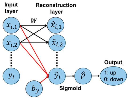
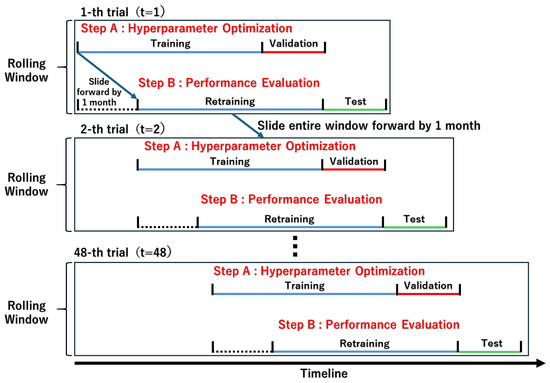
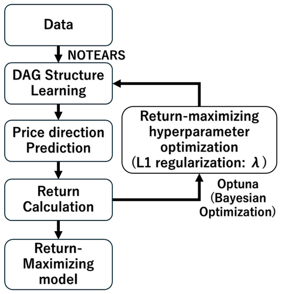
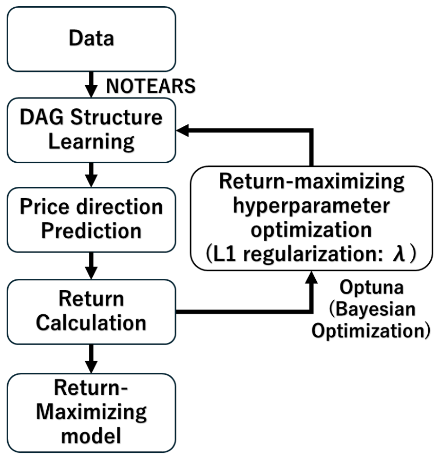
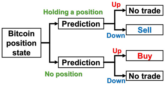
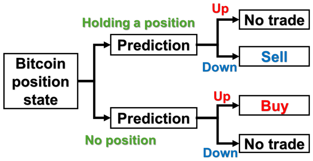
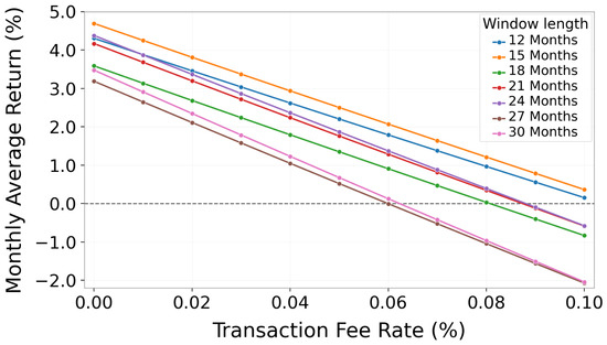
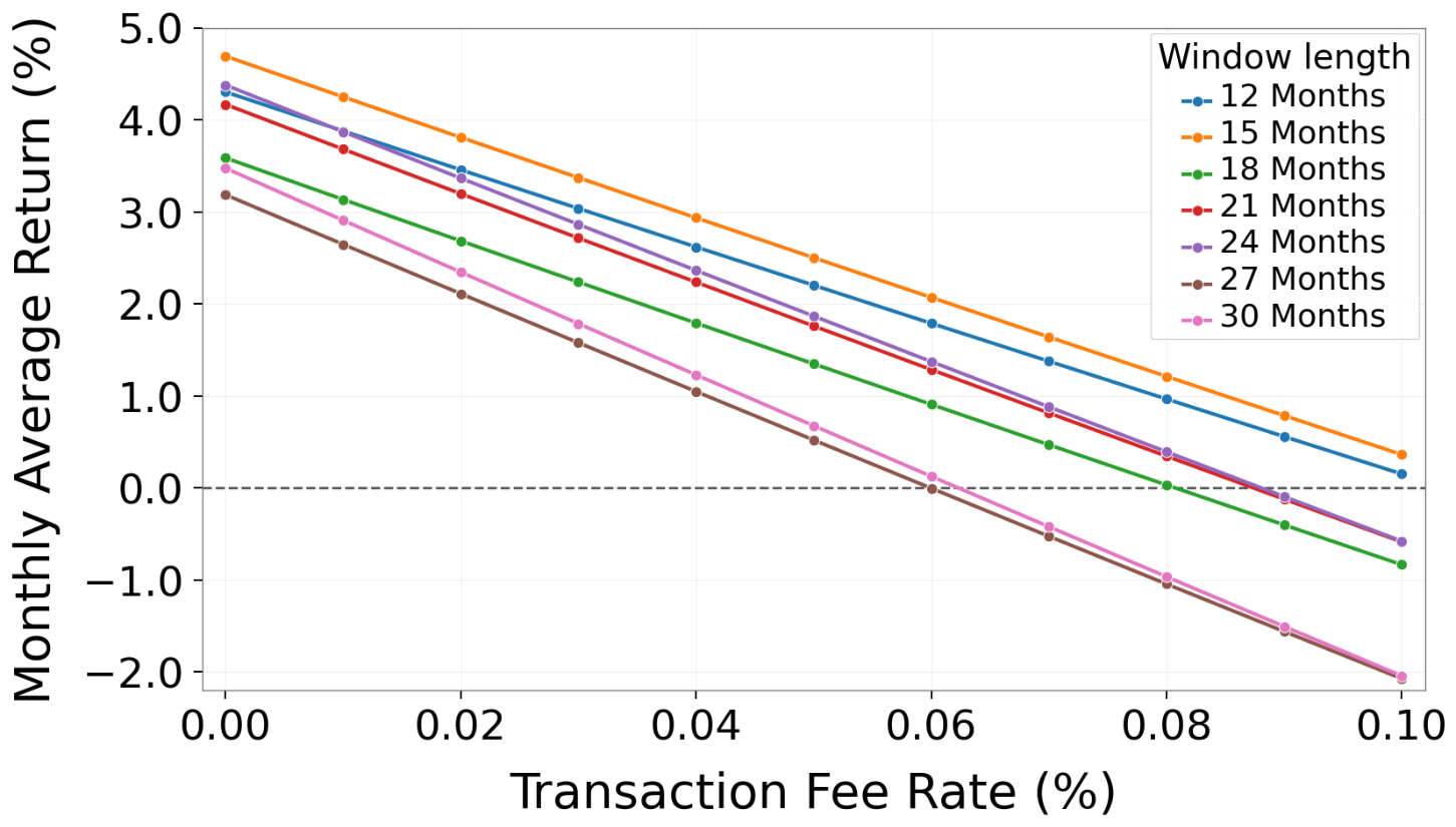
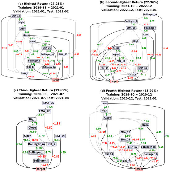
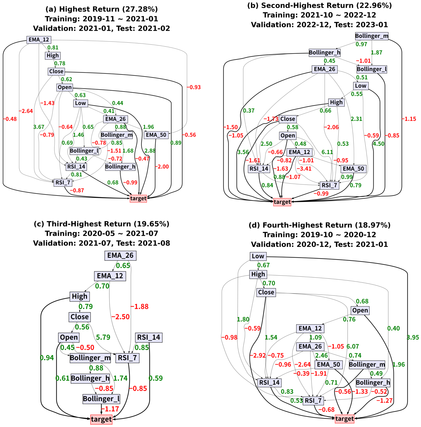

Disclaimer/Publisher’s Note: The statements, opinions and data contained in all publications are solely those of the individual author(s) and contributor(s) and not of MDPI and/or the editor(s). MDPI and/or the editor(s) disclaim responsibility for any injury to people or property resulting from any ideas, methods, instructions or products referred to in the content. |
© 2026 by the authors. Licensee MDPI, Basel, Switzerland. This article is an open access article distributed under the terms and conditions of the Creative Commons Attribution (CC BY) license.