


Highlights
What are the main findings?
- Transfer learning based on the UATL_adaBiGRU technique is robust for the air pollutants prediction task in the data poverty region.
- The proposed uncertainty-aware adaptive TL_adaBiGRU model results are promising for data-scarce regions, as they provide uncertainty quantification and explainable AI capabilities.
What are the implications of the main findings?
- Our study fills an existing gap in the literature through the proposition of an adaptive transfer learning model that is conceptualised on the adaBiGRU technique, which could improve upon legacy-based deep or machine learning systems in South Africa and worldwide.
- Practically, the finding implies that using hybrid model to predict air pollution ensure a more reliable and action-based insight.
Abstract
South Africa faces significant challenges in monitoring air pollution from different provinces due to the sparse nature of the sensor network and heterogeneous pollutant sources. Notably, some provinces continue to record a limited amount of data on air pollution, thus making monitoring in those locations problematic. Fortunately, the capabilities of deep learning models to facilitate effective monitoring in data-scarce locations have been highlighted by researchers; however, these models within the context of transfer learning still lack transparency and uncertainty quantification. Using air pollutants and meteorological factors, this study proposes a transfer learning model for particulate matter (PM2.5) prediction in a data-scarce region. This transfer learning (TL) model leverages an adaptive Bi-directional Gated Recurrent Unit (adaBiGRU) with explainable artificial intelligence (xAI) and uncertainty quantification (UQ) to provide a novel uncertainty-aware adaptation transfer learning (UATL_adaBiGRU) model for a data-scarce location. Variant models based on the adaBiGRU technique, such as the temporal convolution network adaBiGRU (TCN-adaBiGRU) and domain-adversarial neural network adaBiGRU (DANNadaBiGRU), are presented as comparative models. The performance evaluation metrics are root mean squared, R2 score and mean squared error. The R2 score of pre-trained models in source domain is adaBiGRU (0.888), DANN_adaBiGRU (0.7788) and TCN_adaBiGRU (0.876). Furthermore, other comparative TL models include GRU (0.898), MLP (0.802) and adaptive LSTM (0.886). Afterwards, the pre-trained baseline model (adaBiGRU) was fine-tuned in the target domain dataset and the unpromising result contributed to the proposition of the UATL_adaBiGRU model for a data-scarce location, with R2 score of 0.9618. Uncertainty assessment metrics results were also presented for the proposed model. Ablation assessment demonstrates that each component of the UATL_adaBiGRU contributes to enhancing the predictive performance. Again, the Diebold–Mariano (DM) test statistic demonstrates a statistically significant difference between baseline model and UATL_adaBiGRU model. Finally, the local interpretable model-agnostic explanation highlights multi-scaled features as contributing towards the prediction of PM2.5 in the target domain. In view of this result, model fine-tuning is strongly recommended to enhance the robustness of the proposed uncertainty-aware adaption model in data-limited regions in South Africa.
Keywords:
adaptive bi-directional gated recurrent unit (adaBiGRU); explainable artificial intelligence (xAI); temporal convolution network (TCN); Monte Carlo dropout (MCD); uncertainty-aware adaptation transfer learning (UATL); uncertainty quantification (UQ); local interpretable model-agnostic explanation (LIME) 1. Introduction
Air pollution is one of the global environmental risks robbing people of their lives and stretching the health sector’s human resources [1]. It greatly impacts climate change, and causes public health risk and risk to individuals’ health [2]. Over the past decades, considerable efforts have been dedicated to the regulation of air pollutants and monitoring. While countries struggle to deal with the impact of air pollution on their environment, researchers are exploring methods to assess the extent of computational models in air pollution analysis. From practitioners’ perspectives, monitoring air pollution is subject to faulty devices, vandalism of air monitoring devices and others. Though developed nations have the necessary technical expertise and resources to address most unfolding challenges; on the contrary, developing nations may lack the necessary resources to address the challenges.
Currently, there is an increasing reliance on data-driven models to support the automation of air monitoring and analysis processes to find emerging hotspots. While there is no single data-driven model for air quality analysis, there is equally no single model to guarantee the best result, thus leading to open research questions on the extent of data-driven models in air pollution level prediction. The current trend is that, instead of developing a model from scratch, one can adopt a model with a few modifications and then apply it to solve emerging challenges. In this regard, while domain adaptation strategies play an important role in model adaptation, the lack of data to adequately train models hampers its use. For instance, a faulty device is unlikely to generate data to train a model; however, data can be leveraged from another location to facilitate the training of another model. Again, in South Africa, data scarcity challenges are due to vandalism, load shedding, and faulty air monitoring devices, among other factors, which affect regions where air monitoring stations are domiciled [3]. Thus, suggesting the transferability of models from data-rich locations to data-poor locations is imperative. Therefore, transfer learning (TL) is one of the approaches to address data scarcity in different regions. TL can reduce data requirements and speed up model training for a target location [4].
Transfer learning (TL) is a machine learning technique that is framed on knowledge gained and shared to undertake a domain-specific task [5]. This technique has emerged as a data-driven approach to address the frequent data scarcity challenges in air quality prediction. Though the transfer learning technique is affected by domain shift challenges that introduce risk of uncertainties in a target location, it provides some certainty of the model’s performance and generalisation across target locations. Furthermore, researchers suggest that hybridization of models for transferring learning-specific tasks provides a robust model with pre-trained weights from data-rich locations that are fine-tuned to meet the underlying model architecture of a “data-limited” location.
The Centre for Global Change at Sol Plaatje University in the Northern Cape, Kimberley, has identified data insufficiency as a major gap [3,6], which influences its drive to develop effective machine learning-based models for the air pollutants prediction task for data-scarce locations. By leveraging available worldwide global air pollutant data of major cities in the world, an uncertainty-aware adaption transfer learning model is developed for data-scarce locations in South Africa to predict the common air pollutant (that is, PM2.5 concentration). While the explainable artificial intelligence (xAI) technique is integrated into the proposed model to provide explainability and transparency, uncertainty quantification further enhances the trust by providing the range of possible outcomes that might affect the trustworthiness of the transfer learning model, given the domain shift and data scarcity challenges of the target location. This study provides a robust transfer learning methodology to fill the data scarcity gap. The remaining sections are organised as follows: Section 2 presents the literature review, Section 3 presents the methods and materials, Section 4 presents the experimental settings, Section 5 shows the experiment results, Section 6 shows the discussion, and the conclusion and future direction are presented in Section 7.
2. Literature Review
This section reviews xAI and transfer learning models specifically for air pollution prediction in data-scarce locations. The insight gained helps in identifying methodological gaps and proffering practicable solutions with theoretical underpinnings.
2.1. Explainable Artificial Intelligence (xAI) and Transfer Learning Approaches
Explainable AI is principled on enhancing the model’s transparency in any given computational task. While the concept is gaining momentum in several real-world tasks, less is known of its use in transfer learning for data-scarce locations. Artificial intelligence models are known to provide less information about how decisions are arrived at by models, thus making AI models behave like a “black box”. In air pollution applications, stakeholders are keen on knowing the impact of various parameters to arrive at a decision that satisfies multiple stakeholders. One of the challenges associated with deep learning models or artificial intelligence models is their black-box nature, which hampers their general use in organisations. Various xAI models have been proposed to help understand models’ behaviour, and this research seeks to explore those models, especially because of their commonality within the research fraternity.
2.2. Uncertainty Quantification in Transfer Learning Models
Uncertainty quantification provides a clear context for a problem domain in air quality data analysis. When applied in deep learning models, it enhances trust and the use of deep learning models among stakeholders of an organisation [7]. Some of the approaches to improve uncertainty quantification include the use of probability, such as Monte Carlo, and Bayesian methods, to reduce the risk-based decision process of models. Uncertainty risk could arise from the choice of the model’s architecture and parameters, which may create domain shift and introduce bias that could impact models’ reliability in the target domain. In this regard, when the uncertainty quantification approach is introduced in transfer learning, it ensures transparency when models or weights are transferred to data-scarce locations. Normally, the time horizon that exists between the source and target domains could introduce some uncertainty in the model’s behaviour. For instance, while models used in short-range forecasting tend to have low uncertainty, long-range forecasting models have a high level of uncertainty. Thus, this impacts the accuracy of models, in a sense that short-range models have high accuracy, whereas long-range models have low accuracy. Understanding these dynamics gives more insight into model development, leading to the exploration of a more ideal model for any air pollutant predictive task.
2.3. Air Pollution Transfer Learning Models
The transfer learning method helps to address the data limitations in air quality prediction. The idea of transfer learning is based on learning by experience, where the knowledge gained is transferred to solve the prediction task of another similar location. Such knowledge is in the form of models where the task, domain and probabilities are used to represent transfer learning. The ensemble technique is among such models for multiple-sourced transfer learning to mitigate the data shortage or insufficiency issues. Again, transfer learning leverages pre-trained models developed using large-scale datasets to enable the transfer of learned features from one task to another similar task [8]. By using transfer learning, data from one location can be used to predict another location.
Transfer learning has become very crucial in machine learning due to the challenges of machine learning models, which are basically data insufficiency, computational limitations, and a mismatch in the distribution of data [9]. The categories of transfer learning are transductive, inductive, unsupervised, cross-modality and negative or positive. Moreover, each of these categories is grouped into four types of learning: learning by instances, features, parameters, and relations. Multi-layer perception (MLP) is one of such models used to transfer pollutant data across multiple locations to make predictions in another location [4]. Again, models like LSTM, Convolutional Neural Network (CNN) and transfer learning methods have also been proposed [10]. The TL model, such as the TransNet framework, has been used for prediction under data-scarce scenarios while addressing cross-domain adaptability (Mu, Li [11]). Likewise, the transformer-based TL framework (TLT) has been leveraged for long-term water quality prediction (Peng, Wu [12]). In the context of smart buildings, TL has been used to improve energy load prediction, occupancy detection, and building dynamics modelling by leveraging knowledge transfer across related environments, highlighting the potential for efficient control systems (Pinto, Wang [13]).
In transfer learning, when geographic information is required to aid models to effectively capture the spatial features among different monitoring locations [14], the spatial attention module (SAM) is employed for the spatiotemporal feature extraction, whereas the CNN model captures the target domain information and their relationship with other source domains. Furthermore, when transformer models are added to such models, they could capture the long-distance time relationship between similar geographic monitoring locations. In these regards, hybrid ensemble and transfer learning models have played key roles in building resilient transfer learning models for air pollutant prediction if target monitoring stations are data-deficient [15].
Recent studies have explored TL for spatiotemporal modelling and adaptation in data-limited scenarios. For example, a dynamic graph that integrates short- and long-term dependencies in air quality prediction (Chen, Xia [16]), while heterogeneous TL (HTL) with perceptive-pruning and fine-tuning strategies has been applied to handle the challenges posed by low-frequency monitoring stations (Yang, Peng [17]). Moreover, multi-source variational mode TL (MSVMTL) integrates decomposition and clustering strategies to optimise prediction at sites lacking sufficient historical air pollution data (Yao, Ling [18]). Fong, Li [19] indicate that transfer learning and pre-training models provide a surety to address the data insufficiency issues, and when a pre-trained model is applied in a target location, it could effectively predict with a limited amount of data [20]. However, data pipelining models introduce uncertainties which impact the performance of models and reduce trust in model adoption [21]. Basically, a data pipeline explains the flow of data through different stages, including data acquisition, standardisation and its analysis. These uncertainties are either driven by randomness or a lack of knowledge about a domain.
It has been highlighted that more advanced deep learning models are good at prediction but need more data for training, and due to the data deficiency challenges at new monitoring stations, transfer learning can predict air pollutant concentration at new monitoring stations even if data is limited [22]. The nonlinear and non-stationary behaviour of pollutants (PM2.5) makes future prediction challenging in the short term [23]. Thus, the VMD enhanced with the correntropy criterion, SVR and state transition simulated annealing model was proposed to address this nonlinearity and non-stationary behaviour. Though the decomposition approach is effective at capturing local and temporal features, its computational time and model complexity are some challenges. Thus, a deep learning-based system that considers meteorological and air pollutant factors was applied using an arithmetic optimisation algorithm (AOA), double-layer bi-directional GRUs (DBGRU), and a mixture density network (MDN) (Che, Hu [24]). It involves feature selection using maximum information coefficient (MIC), decomposition using the complete ensemble empirical mode decomposition with adaptive noise (CEEMDAN) algorithm, classification, and compression of decomposed components using entropy–Huffman tree compression. The reconstruction of data based on entropy–Huffman tree compression improves accuracy and decreases model training.
While private companies establish air monitoring stations to compensate for data gaps, in practical cases, missing data features cannot be accounted for in air pollution data. While an approach to address this has been suggested [25], data heterogeneity distribution over different networks can be the cause of incomplete data. The general Gaussian mixture model (GMM) approach was proposed to model both private and public data distribution components. Thus, a distributed personalised expectation-maximisation approach based on knowledge transfer (KT-dpEM) was proposed to estimate the parameters of the general GMM. Missing data is imputed based on the posterior conditional mean. It is indicated that due extended time span which monitoring stations are not operational, data would be lost, and this can be addressed with transfer learning [26]. Other proposed transfer learning models include a transfer learning-based stacked BiLSTM (TLS-BiLSTM) model to perform air quality prediction at new air pollution stations [27].
Jairi and Ben-Othman [4] applied MLP as a transfer learning approach to learn across different air pollutants within the same monitoring station using large data on air quality concentrations. They suggested that using transfer learning improves model accuracy and it also requires much less fine-tuning in the target domain. Again, fine-tuning pre-trained models enhance performance of any prediction, thus suggesting that model fine-tuning is task-specific. Ma and Wang [6] suggested deep learning models (LSTM, RNN, weighted LSTM, BiLSTM and GRU) as very vital in selecting an internal feature of data and their correlations. Furthermore, machine learning models such as MLP, SVM and Random Forest Regressors (RF) are helping to design effective air pollutant predictive models. Some literature suggests that RF continues to be the most dominant machine learning model, recording an accuracy of 99% in the air pollution predictive task [28], highlighting the use of DL and ML in creating air pollutant models. Unfortunately, these models are unable to perform optimally when there is limited data available to train them. Thus, when applied to the target location, their performance is problematic. The two-stage attention-based model (TL-AdaBiGRU), which is principled on transfer learning, was proposed to enable model learning from multiple head external attention features and to capture the complex nonlinearity in pollutant data. While Dhole and Ambekar [29] stated that DL models address data limitation problems, the lack of resources or personnel to collect meteorological and environmental data compounds the challenge, thus creating a crippling data-insufficient issue. These challenges further stress the need for an ensemble method for multi-source transfer learning.
In developing nations where limited air monitoring stations are a challenge, the need for a deep citywide multisource data fusion (i.e., FAIRY) model becomes more relevant (Chen, Long [30]). Though this FAIRY model used image data from the multisource, it highlights high-resolution data acquisition for an effective prediction. In this regard, graph based models with time-frequency transformation (that is, Frequency Enhanced Decomposed Temporal Convolution Network (Fed-TCN) (Huang, He [31]) was proposed to enable accurate long-term pattern prediction for different air pollutants, such as PM2.5, PM10, nitrogen dioxide (NO2), carbon monoxide (CO), sulfur dioxide (SO2) and ozone (O3). Research shows a growing trend of the application of DL models for TL, which are summarised in Table 1.
Table 1.
Summary of transfer learning models for air pollution.
While having multiple air monitoring stations provides an avenue to compensate for the data gap, the model’s domain adaptation and uncertainty quantification could facilitate transfer learning and prediction. Several transfer learning models have been highlighted, such as ML [23] and DL (TLS-BiLSTM [27], double-layer bi-directional GRUs (DBGRU) [24]) for different air pollution tasks. Again, this suggests the application of advanced deep learning models for data deficiency in target monitoring stations. Thus, transfer learning [22] or multi-source transfer learning mechanisms [50] are more relevant. Researchers such as Cheng and Fang [32] have hybridized GAN with other models within the context of TL for spatiotemporal predictions. It is revealing that the collective strength of DL and ML models provides a robust approach to dealing with data scarcity issues. While model hybridization compensates for each model’s strength or weakness, it also calls for more transparency in a model’s predictive outcome. It is worth noting that TL models have also been applied in other problem domains (e.g., water, energy and federated learning), which demonstrates their predictive robustness. Table 2 shows the TL models applied in other domains.
Table 2.
Transfer learning models in other research domains.
While our study highlights TL techniques in air pollution tasks and other problem domains, it also highlights methodological challenges (Table 3) for further research.
Table 3.
Methodological gaps, solutions and theoretical underpinnings.
The key insight gained from this review is that the integration of xAI into the TL model provides a unique method for providing experts with some explanation of a model’s prediction for a specific task. Some advantages of TL models can include domain adaptability capability under data scarcity conditions. Transfer learning with fine-tuning is considered a robust technique in air pollution analysis [56]. However, uncertainty quantification remains a non-integral part of TL models, thus making it a challenge to understand the extent to which architectural configuration contributes to TL model fine-tuning in air pollution-related tasks and their geographical data variability. Therefore, TL models should consider such challenges to provide adequate expert knowledge relative to predicting air pollutants. Therefore, a hybrid framework that combines domain adaptation, xAI, and multi-source TL offers theoretical grounds and a practical guide to improve a model’s reliability and actionable insights for environmental decision-making. The literature review acknowledges the existence of several transfer learning models which include GRU, TCN, adaptive LSTM, DANN, and CDAN.
3. Materials and Methods
In this study, a transfer learning (TL) model was proposed, which used knowledge gained in terms of a pre-trained model from a data-rich location to predict the concentration level of air pollutants (that is, PM2.5) in a data-scarce location, without having to train the model in the target location from scratch. This approach helped to generalise the prediction in the target location. Figure 1 shows the TL model development phases which include data acquisition, pre-processing, analysis and visualisation.
Figure 1.
Proposed transfer learning framework.
Based on the framework (Figure 1), the steps to develop the adaptive TL model are as follows: source data preprocessing; model creation and training on data-rich location; evaluation on source data; transfer learning of pre-trained model; model fine-tuning for the target location; uncertainty quantification using Monte Carlo dropout on the target location data; and explainability. The uncertainty estimates generated via MC dropout are employed as uncertainty feedback signals during the target domain adaptation to support the uncertainty-aware transfer learning strategy. In this regard, any high-uncertainty samples are assigned a lower confidence weight during the optimisation stage, while the uncertain prediction regions are identified for an adaptive fine-tuning to enhance the model’s robustness, thus helping to revise the transfer learning framework and help to integrate predictive confidence into the adaptation process rather than treating uncertainty solely as a descriptive metric. During fine-tuning of the transfer learning model, the bidirectional GRU layer was frozen, and the output layer was retrained with a smaller learning rate (0.0005). The layer-freezing strategy for the transfer learning allows retraining of pre-trained knowledge and allows stable feature extraction and adaptation of the final layers. Furthermore, the dense layer with the L2 kernel regularisation strategy was employed. Thus, helping to build the Uncertainty-Aware Robust Model with Regularisation.
Within this study, robustness is principled on the model’s ability to perform reliably well under noisy data, missing features, domain shift and unseen environmental features. On the contrary, lack of feedback mechanism makes a model prone to wrong predictions and possibly overfit transferred knowledge. Thus, the uncertainty-aware adaptation transfer learning (UATL) strategy is a transfer learning strategy that explicitly integrates predictive uncertainty as a feedback mechanism for domain adaptation and optimisation process to enhance the model’s reliability, generality and robustness across heterogeneous domains.
3.1. Dataset
In this paper, two available datasets were used; that is, the dataset from the source (that is, data rich location) and the target location data. The source location dataset consists of hourly air pollution data recorded in 2026 from eight major global hubs. This dataset covered the period from October 2025 to January 2026 (Smog Season, where PM2.5 reached a hazardous level) and contains 17,472 records with zero missing values. The target location dataset (data-scarce location) contains an hourly dataset on Cape Town, South Africa, with zero missing values. The target dataset covered the period of 2025. The target domain dataset included environmental and air pollutant recording, whereas the source domain recorded only air pollutant data. In this research, an input sequence length of 24 past readings was used to ensure adequate training. The PM2.5 concentrations are measured in ug/m3.
Inconsistency in feature dimension space between the source and target domain is a factor that could negatively impact the transfer learning model. To address the inconsistency in the feature space, the study harmonised the data from the source and target domain into a common feature space before model training and transfer. Only the shared air pollutant variables present in both domains were re-trained for transfer learning. Features were normalised and preprocessed independently in each domain to prevent any information leakage between datasets. Additionally, the transfer process was done using parameter transfer to avoid any possible direct data mixing. In this regard, our model was initially pre-trained on the source-domain dataset and subsequently fine-tuned with only the target-domain training dataset. Thus, no target-domain test samples were exposed during the source-domain training process or parameter initialisation, thereby preventing possible data leakage.
3.2. Adaptive Model Formulation
Step 1: Initialisation.
Let , representing the input feature vector at time t, and n is the number of features, which are the air pollutants and meteorological factors from both source and target location. That is, .
: PM2.5 concentration at time t.
Dataset: , , where S is the source (data-rich locations), and T is the target domain (limited data).
Model parameter: learning rate, dropout rate, epochs, CRPS weight.
Step 2: Bidirectional GRU Formulation for backward and forward propagation is expressed as follows:
Thus,
Candidate Hidden state (memory information):
Hidden state update (previous memory and new candidate information):
Step 3: Adaptive attention mechanism focused on attention score (termporal feature importance), adaptive attention weight (that is, the normalised feature importance scores) and adaptive context vector (that is, weighted temporal representation) are expressed by
where represents the BiGRU hidden representation, is the adaptive weighted matrix, v is the trainable attention vector.
Step 4: The transfer knowledge learned in the source region to the target domain is expressed by
where represents the source weight which was transferred to target domain . Strategies to achieve this knowledge transfer includes freezing lower BiGRU layers and fine-tuning the upper layers and the attention layer. This then outputs the initialised target adaBiGRU model’s weights.
The transfer learning technique is based on the adaptive Bi-directional Gated Recurrent Unit (adaBiGRU). This technique helped to capture complex nonlinear relationships in a time series air pollutant dataset. The adaBiGRU is conceptualised on learning from both forward and backward directions within a sequence. It utilises three key strategies: pre-training, fine-tuning and knowledge transfer. Firstly, the pre-trained strategy entailed the training of the transfer learning model in a data-rich location to generate pre-trained weights/models. Secondly, the pre-trained model was then fine-tuned using the limited data in the target location. Lastly, a knowledge transfer strategy referred to when the pre-trained model gained a prior knowledge to understand the underlying patterns, which could improve prediction accuracy in the target domain. The fine-tuning technique focused on the architecture constituents and their hyperparameter value—for example, GRU units, dense units and dropout rates, with their corresponding upper and lower layers. This research innovates transfer learning-based adaBiGRU architecture by combining the bidirectional GRU with adaptive attention weighting to improve the long-term temporal dependency of feature learning and contextualise representation learning for data scarce region. By so doing, enhancing the prediction accuracy in air prediction task. In this research, our strategy was to first pre-train a model on the source dataset to establish the baseline performance weights and then transfer the learning representation of the model’s architecture as weights to the target domain.
3.3. Uncertainty Quantification for Transfer Learning
The uncertainty quantification is an approach to assess the level of confidence in a model to perform an accurate predictive task. The approach relies extensively on statistical methods, thus ensuring an objective assessment of a model. In this study, the approach assesses the confidence level of a model in a new location or target location or data-scarce location. Mostly, transfer learning-based deep learning models often struggle to accurately predict outcomes in new locations due to domain shift or data variability, which limits their application in any air pollution task. By equipping transfer learning models with uncertainty quantification capabilities, they can adjust to the underlying data distribution and learning parameters to handle the domain shift in the target location. One of the approaches to handle uncertainty quantification is the Monte Carlo dropout technique, which employs Bayesian inference by random dropout. Uncertainty quantification is necessary because of either data variability in the target location or the choice of the model’s architecture, missing observation, nonlinear atmospheric dynamics and parameters. While data variability looks at the inherent randomness in the data, the architecture looks at the underlying model structure. Therefore, the proposed model considers the choice of model architecture and its parameters, and gives insight into the impact on the prediction of uncertainty in the target data location. The choice of architecture includes GRU units, dense units, and dropout rate, and how they influence the accuracy of prediction and quantified uncertainty. Thus, the MC dropout approach improves the reliability and interpretability of predictions by estimating both the prediction outputs and its associated confidence levels. The workflow of the MC dropout for uncertainty-aware adaptation is expressed by the following steps:
Step 1: Loading weights for baseline model and training the adaBiGRU model with dropout regularisation to fine-tune in the target domain.
Step 2: Keeping dropout active during inference by introducing Bernoulli-distributed random variables over network weights.
where is the dropout mask and p is the neuron retention probability. Thus, the effective weight matrix is expressed by the following:
where W is the original weight matrix, and w is the stochastic weight matrix.
Step 3: Perform T stochastic forward passes by using
where represents the prediction from the Tth stochastic pass, is the randomly sampled dropout weights. Thus, for each target sample prediction:
Step 4: Compute predictive mean (that is expected pollutant concentration).
where is the predictive mean and T is the number of MC samples.
Step 5: Compute predictive variance.
Thus, larger variance suggests higher uncertainty and lower prediction confidence.
Step 6: Compute predictive uncertainty or standard deviation :
where large indicates low confidence.
Step 7: Estimate uncertainty prediction interval (that is, confidence interval estimation for each prediction)
Step 8: Total uncertainty () estimation is expressed using both the aleatoric uncertainty () (that is, inherent data noise expressed in terms of the Negative Log-Likelihood (NLL) loss) and epistemic uncertainty () (that is, model uncertainty variance estimation from MC dropout, which is the predictive mean in the target domain) components as the sum of the variance as follows:
where aleatoric uncertainty ( is expressed by the following:
Then, epistemic uncertainty is expressed by the following:
Step 9: Confidence weight computation:
where β is the control factor, thus converting the total uncertainty into confidence weighting. These confidence weights were tuned to the target domain to ensure dimensionality match. This fine-tuning incorporates the previously calculated confidence_weights from the source domain to give more importance to samples in target domain where the model is more certain, thereby improving overall predictive performance and robustness. The confidence weight ranges between 0 and 1. The resulting model is saved for evaluation. In this regard, highly uncertain value contributes less during adaptation.
The uncertainty-aware adaptation mechanism, in which the MC dropout-derived predictive uncertainty dynamically weights the target-domain samples during the fine-tuning of the adaBiGRU model, therefore helps to directly link the weight to the uncertainty quantification to the adaptation in the target domain.
Step 10: Uncertainty-aware adaptation fine-tuning (that is, uncertainty-weighted MSE) with confidence weight to optimise loss (MSE) in target domain which is expressed by the following:
Step 11: Compute CRPS as follows:
where , represents each MC dropout prediction and is the single true observed target value of PM2.5. M is the total number of predicted values. In this regard, the first part of the equation measures the accuracy of prediction (in terms of the error between and , while the second part of the equation measures the uncertainty (that is, the average absolute differences between all possible pairs of predictions). A lower CRPS value shows better uncertainty calibration. For example, if the CRPS value is 0 then it indicates better prediction accuracy and more reliable uncertainty.
Step 12: Hybrid loss function () seeks to integrate the CRPS into the uncertainty-aware adaptation expression. Thus, the idea is to optimise not only the prediction accuracy but also the quality of the predicted uncertainty distribution. Thus, the objective loss function is expressed as follows:
where controls the contribution of uncertainty within 10−4 and 10−1. Thus, the model was fine-tuned using this objective function, where nill is the Negative Log-Likelihood, which trains the variance head.
Step 13: Create and train UATL_adaBiGRU model with a hybrid loss for prediction.
Step 14: Reliability scoring (R) of the UATL_adaBiGRU model: , where R ranges from highly reliable prediction (that is, 1) and highly uncertain prediction (that is, 0).
Step 15: Perform evaluation and uncertainty calibration assessment.
Step 16: Perform Diebold–Mariano test with the baseline model.
Step 17: LIME explanation.
Step 18: LIME stability index (Ls) is expressed in terms of Spearman rank correlation as follows:
where K is the number of runs, is Spearman rank correlation and LIME produces a feature importance vector as , where the index is categorised as very stable (>0.90), stable (0.75 and 0.90), moderate (0.50–0.75) and unstable (<0.50).
3.4. Evaluation Metrics
The TL models were evaluated with metrics such as root mean squared error (RMSE), R2 score and mean squared error (MSE). While a negative value suggests that the model is not complex and robust, a positive value (R2 > 0.8) shows a complex and robust model. These metrics are expressed in Equations (28)–(30).
where represents the actual value, y represents the predicted value, and N is the number of samples. Coefficient of determination (R2) explains how well model fit the target data, where is the mean of the actual target value, n represents the number of data points.
Furthermore, uncertainty calibration assessment metrics assessed the UATL_adaBiGRU model’s confidence at prediction, using variables such as average uncertainty, prediction interval coverage probability (PICP), mean prediction interval width (MPIW), Expected Calibration Error (ECE), Negative Log-Likelihood (NLL), and Continuous Ranked Probability Score (CRPS). Table 4 shows the description of the uncertainty calibration assessment metrics.
Table 4.
Description of uncertainty assessment metrics.
The performance of the proposed model was compared with existing models such as GRU, TCN_adaBiGRU, adaptive LSTM, DANN_adaBiGRU and CDAN, which were identified in literature as commonly used transfer learning models. The review of literature provides evidence that the existing TL models lack MC dropout for uncertainty quantification. Our proposed model (UATL_adaBiGRU) filled this gap by integrating MC dropout computation for a reliable and robust transfer learning for data poverty regions. Table 5 shows the existing TL models without MC dropout uncertainty quantification and the assessment metric including MSE, RMSE and R2 score.
Table 5.
Existing TL models without MC dropout.
To ensure the statistical rigour of the proposed model in relation to the comparative models, the Diebold–Mariano test was conducted to assess the predictive accuracy of the two models. LIME stability is computed to quantify the consistency of the explanation in K multiple runs.
4. Experimental Settings
The model was developed using the Python 3.10 environment because of the ease of implementation of machine learning or deep learning TensorFLow libraries on Google Colab. During the experiment, Intel Core i7 was used with 32 GB RAM on Windows 10 operating system. Table 6 shows the hyperparameter settings of the model.
Table 6.
Models hyperparameter settings.
5. Experiment Results
5.1. Data Exploration
Figure 2 and Figure 3 show the distribution of average PM2.5 concentration levels across the cities in the original world air pollution dataset for cities (source dataset).
Figure 2.
Average PM2.5 concentration per city in the source dataset.
Figure 3.
Frequency distributions of air pollutants in the source dataset.
From Figure 3, the blue lines on each histogram explains the density estimation curve of each pollutant to ensure a more visual display of the distribution. It can be observed that the pollutant concentrations are non-normally distributed and exhibit varying degrees of positive skewness. Furthermore, the long right tails show the presence of occasional extreme air pollution episodes, whereas, the dominant peaks at the lower concentrations show the prevalence of normal air quality conditions in each observation.
Figure 4 shows the correlation matrix of air pollutants in the source dataset.
Figure 4.
Correlation matrix of air pollutants.
Figure 5 shows the distribution of air pollutants available on the target location dataset, which is the data-scarce location. It can be observed that, the blue line on each figure which represents the density estimation curve, demonstrates a smoothed estimate of the probability density function of the data in the target domain. Unlike the histogram, which displays frequencies within discrete bins, the density estimates provides a continuous view of the underlying distribution of each air pollutant, thus, making it clearer to identify the distribution curve, the central tendency, the skewness and the potential multimodal patterns in the data.
Figure 5.
Frequency distributions of air pollutants in target location data set.
The analysed uncertainty quantifications are visualised using the mean of prediction and its standard deviation plot and uncertainty histograms.
5.2. Model Evaluation
The baseline models (Table 7) and their performance are assessed using test data from the source domain with MSE, RMSE and R2 score.
Table 7.
Performance metrics of the baseline pre-trained models in the source domain.
From Table 7, it can be observed that the GRU model guaranteed R2 score of 0.898, while adaBiGRU (0.888), DANN-adaBiGRU (0.779), TCN-adaBiGRU (0.876), adaptive LSTM (0.886), and MLP (0.802). The results show that approximately all the R2 scores > 0.8. However, the GRU model demonstrates superiority by a minimal margin. This implies that the models explain approximately 80 per cent of the variance of PM2.5 concentration level in the source dataset. Furthermore, in terms of the RMSE, GRU guaranteed 11.252, adaBiGRU (11.7968), DANN-adaBiGRU (16.5905), TCN-adaBiGRU (12.4370), adaptive LSTM (11.9117) and MLP (15.6977). This result shows how the predictions are far from the actual PM2.5 concentration. Figure 6, Figure 7, Figure 8, Figure 9, Figure 10, Figure 11 and Figure 12 illustrate the models’ prediction vs. the actual PM2.5 in the test data.
Figure 6.
adaBiGRU model prediction vs. actual data.
Figure 7.
Adaptive LSTM model prediction vs. actual data.
Figure 8.
GRU model prediction vs. actual data.
Figure 9.
MLP model prediction vs. actual data.
Figure 10.
TCN attention-enhanced BiGRU model prediction vs. actual data.
Figure 11.
DANN_adaBiGRU model prediction vs. actual data.
Figure 12.
CDAN model prediction vs. actual data.
Furthermore, the study also demonstrates the extent to which the pre-trained model generalises to the target domain data and presents the results in Figure 13, Figure 14, Figure 15, Figure 16, Figure 17, Figure 18 and Figure 19.
Figure 13.
Pre-trained adaBiGRU prediction vs. actual values on target data.
Figure 14.
Pre-trained adaptive LSTM prediction vs. actual values on target data.
Figure 15.
Pre-trained GRU prediction vs. actual values on target data.
Figure 16.
Pre-trained MLP prediction vs. actual values on target data.
Figure 17.
Pre-trained TCN adaBiGRU prediction vs. actual values on target data.
Figure 18.
Pre-trained DANN-enabled adaBiGRU prediction vs. actual values on target data.
Figure 19.
Pre-trained CDAN-enabled adaBiGRU prediction vs. actual values on target data.
During the fine-tuning of pre-trained models in the target domain, the study focused on the model’s architecture and its hyperparameter. Strategies such as layer freezing and regularisation were also employed. In view of this, the models were fine-tuned to evaluate the prediction performance (see Table 8). The fine-tuning enables a systematic exploration of the hyperparameter space to assess each model’s performance and identify the most effective configuration. Table 8 shows the performance of the fine-tuned models.
Table 8.
Performance metrics of the TL models in target domain.
The study adopted the grid search-based approach subject to the hyperparameter setting to fine-tune the adaBiGRU (baseline model) and included also the uncertainty estimation to enhance its performance, thus proposing the enhanced uncertainty-aware adaption adaBiGRU model referred to as UATL_adaBiGRU model. It can be observed that the proposed UATL_adaBiGRU model’s architecture, after the grid search, generated gru_units (64), dense_units (32), dropout_rate (0.1), learning_rate (0.001), batch_size (32), early_stopping_patience (7) and L2_strength (0.001). The R2 score is 0.9618 and the best weight for this architecture configuration was generated. However, the existing models had negative R2 scores. Figure 20 shows the proposed UATL_adaBiGRU model’s prediction vs. actual values in the target domain dataset.
Figure 20.
Fine-tuned UATL_adaBiGRU model’s prediction in the target domain.
After fine-tuning the proposed model in the target domain with the hybrid loss function value, uncertainty assessment was performed (Table 9).
Table 9.
Uncertainty assessment.
Table 9 shows epistemic uncertainty (2.86 × 10⁻³), aleatoric uncertainty (5.406 × 10⁻²), total uncertainty (5.415 × 10⁻²), confidence weight (0.9718) and total loss (1.78 × 10⁻³). It can be observed that the mean epistemic uncertainty is low, indicating that the model is confident about the learned parameters, whereas the mean aleatoric uncertainty suggests that the model has extremely high noise or uncertainty in data. Thus, the mean aleatoric uncertainty is the dominant attribute of the proposed model. The confidence value (0.9718) suggests that the proposed model assigned a high confidence to the prediction. Table 10 shows the uncertainty calibration metrics in terms of prediction interval coverage probability, mean prediction interval width, Expected Calibration Error, Negative Log-Likelihood and mean CRPS.
Table 10.
Uncertainty calibration assessment.
From Table 10, it can be observed that the CRPS is 1.6098, which demonstrates good performance in the target domain and reliable predictive distributions. The UATL-AdaBiGRU model achieved complete interval coverage (PICP ≈ 1.0), suggesting that all the observed PM2.5 concentration values were captured within the prediction range. Contrarily, the corresponding MPIW value was extremely large (~1686 μg/m3), indicating that the uncertainty estimates were overly conservative. Figure 21 shows the time series prediction and coverage probability plot of the UATL_adaBiGRU model.
Figure 21.
Time series prediction and coverage probability plot.
With respect to the time series predictions (Figure 21), it can be observed that the actual PM2.5 predictions fluctuate mostly between 20–80 μg/m3 (represented with a black line), while the predicted mean with uncertainty exhibits the general trend of observation. This result suggests there is no bias; therefore, the UATL_adaBiGRU model’s predictions are within the observed trend and it is learning useful patterns. Furthermore, in respect of the temporal calibration, the MPIW is extremely large, indicating an over-conservation of uncertainty estimates, which may be due to the large log variance. Figure 22 shows the training and validation plot of the UATL_adaBiGRU model.
Figure 22.
UATL_adaBiGRU model’s training and validation loss curve.
From Figure 22, validation loss of 2.658 × 10⁻³ was recorded. It can be observed that the validation loss decreases at each epoch, suggesting a successful fine-tuning with the hybrid loss value. Therefore, effective transfer learning and good convergence performance were achieved without any evidence of model overfitting.
5.3. Explainable AI: LIME Analysis Results of the Model in the Target Location
This section provides the explainable AI’s results (Figure 23, Figure 24, Figure 25, Figure 26, Figure 27, Figure 28, Figure 29 and Figure 30) obtained by the models in the target location. The results provide insight into important variables that influence the model’s prediction in the target location.
Figure 23.
Fine-tuned adaBiGRU LIME explanation of PM2.5 concentration.
Figure 24.
Fine-tuned GRU LIME explanation of PM2.5 concentration.
Figure 25.
Fine-tuned MLP LIME explanation of PM2.5 concentration.
Figure 26.
Fine-tuned adaptive LSTM LIME explanation of PM2.5 concentration.
Figure 27.
Fine-tuned TCN_adaBiGRU LIME explanation of PM2.5 concentration.
Figure 28.
Fine-tuned DANN_adaBiGRU LIME explanation of PM2.5 concentration.
Figure 29.
Fine-tuned CDAN LIME explanation of PM2.5 concentration.
Figure 30.
LIME explanation of UATL_adaBiGRU model.
From Figure 23, it can be observed that the overall predicted value, using adaBiGRU, is 60.97, which shows that the model is influenced by both the orange (positive) and blue (negative) features. This suggests that PM2.5 prediction is strongly influenced by lagged PM10 concentration and the gaseous pollutants (e.g., NO2 and O3). Again, the weekend and hour indicators also reduce predicted PM2.5 concentration in the target location, and this pattern of emission and temporal dynamics impacts the predicted PM2.5 concentration.
Figure 24 shows the LIME explainer for the GRU-based transfer learning model. It can also be observed that the predicted value of PM2.5 is 46.86. Meanwhile, the predicted value ranges from −3.35 (min) to 142.41 (max).
Figure 25 shows the LIME explanation for the MLP transfer learning model. It can be observed that the predicted value is 43.75. The predicted value is enclosed in the range min (8.94) and max (118.18). So, this is a moderate PM2.5 concentration level. It can be suggested that, based on the dataset, PM2.5 may increase on weekends. Again, time-related factors such as late-night hours could be seen as impacting the prediction, which implies that the time-related factor reduces the PM2.5 prediction. Furthermore, PM10 also contributes to both reducing and pushing the prediction of PM2.5 to the predicted value. The over-reliance on time-related factors in this model is a concern, suggesting the lack of robustness of this model.
Figure 26 shows the LIME explanation for the adaptive LSTM-based transfer learning model. It can be observed that the predicted value is 50.33. The predicted value is enclosed in the range min (19.54) and max (133.13). It can be observed that PM10 both pushes and reduces the prediction of PM2.5. Again, time-related and gaseous pollutants (CO, O3 and NO2) contribute to the recorded predicted value.
Figure 27 shows the LIME explanation for TCN_adaBiGRU-based transfer learning model. It can be observed that the predicted value is 35.96. The predicted value is enclosed in the range min (20.30) and max (118.80). PM10 is a key determinant that influences the prediction of PM2.5 of the recorded predicted value both positively and negatively. Again, gaseous pollutants (CO and NO2) contribute to reducing the recorded predicted value, whereas gaseous pollutants (CO, SO2, NO2 and O3) contribute to pushing the prediction up to the recorded value. The results suggest that PM2.5 prediction is strongly influenced by both short-term and long-term lagged PM10 concentration, where PM10 at time (t-1) shows the highest positive contribution. However, lower recent PM10 values (t0–t4) exert a dominant negative influence, resulting in a moderated prediction. Temporal features, particularly day of week, indicate reduced emissions during weekends.
Figure 28 shows the LIME explanation for DANN_adaBiGRU-based transfer learning model. It can be observed that the predicted value is 48.18. The predicted value is enclosed in the range min (19.75) and max (125.86). It can be observed that NO2 contributes to reducing the prediction, whereas air pollutants (PM10,) and (CO, SO2, and NO2) push the prediction of PM2.5 to the recorded level of concentration. Furthermore, time-related factors also contribute to reducing the concentration of PM2.5 in the target location.
Figure 29 shows the LIME explainer of CDAN model. It can be observed that the model relies heavily on the temporal features like day of week and hour of day instead of the air pollutants. These temporal features push the prediction of PM2.5 concentration down.
Figure 30 shows the LIME explainer of the proposed UATL_adaBiGRU model. The integration of LIME explainer gives insight into the mean prediction output (that is, mean_output) to identify the most influential features in the input that contributes to the PM2.5 concentration prediction. It can be observed that both temporal features and air pollutants (e.g., PM10 and Ozone) contributed to pushing the prediction of PM2.5 further downwards. The red vertical bars indicate features that contribute towards pulling down the PM2.5 concentration prediction whereas the green bars are features that contribute to pushing the PM2.5 concentration.
Table 11 provides a summary of the components included on the TL models.
Table 11.
Components of the comparative models.
The LIME was employed as a post hoc explainable and does not influence the model’s training and predictive performance.
Table 12 presents the ablation assessment regarding the contribution of each component to the proposed model’s performance, specific to the target domain.
Table 12.
Ablation assessment of UATL_adaBiGRU model.
Table 12 shows the contribution of components toward predictive performance. The UQ component contributes to the predictive reliability and accuracy of prediction, and the xAI enhances interpretability through feature attribution analysis. In this regard, both the UQ and xAI are intended to improve trustworthiness and transparency. The uncertainty calibration assessment metrics, including CRPS, PICP, MPIW, NILL and ECE, yielded results for the UATL_adaBiGRU model. It can be observed that including the uncertainty estimation strategy enhanced the UATL_adaBiGRU model’s performance, as indicated by RMSE (3.2847), MSE (10.7895) and the R2 score (0.9618). Meanwhile, the hyperparameter tuning strategy also contributed to improving the adaBiGRU model’s performance, yielding RMSE (4.2541), MSE (18.0971) and the R2 score (0.9347). This result suggests that the proposed model is capable of reducing the error between the observed and predicted variable (that is, PM2.5) in the target domain. Meanwhile, the LIME stability index of 0.85 signifies model stability. Furthermore, Table 13 presents the Diebold–Mariano test statistics on the baseline and UATL_adaBiGRU models.
Table 13.
Diebold–Mariano (DM) test.
The Diebold–Mariano (DM) test, as a statistical strategy, was employed to compare the UATL_adaBiGRU with the baseline model (that is, adaBiGRU). With this approach, the statistical significance between both models was computed at p-value < 0.05. To perform the DM test, two hypotheses were expressed as follows:
- Null Hypothesis (H0): Both models have equal prediction accuracy.
- Alternative Hypothesis (H1): One model is significantly more accurate than another.
From Table 13, the result shows a DM statistic of 28.7111, which is extremely high, and a p-value of 0.000. The result suggests rejection of the null hypothesis because of the statistically significant difference in the accuracy between UATL_adaBiGRU and the baseline (adaBiGRU) model at a 0.05 significance level.
6. Discussion
The explainable AI provides the needed insight to stakeholders within the air pollution operation chain. This helps in knowing important variables and how they push the model to make predictions within the target domain. One of the main challenges with the existing transfer learning model is the ability to provide explanations, which benefits its stakeholders and provides some level of transparency on how deep learning models are influenced by input parameters. Mu and Li [11] indicate that cross-domain adaptability of the transfer learning model remains a key issue in air pollution analysis. While several models to address domain shift have been proposed, they are deficient in providing insight into the uncertainty quantification, which limits the utilisation of transfer learning models in air pollution-related tasks. Our approach contributes significantly by providing a spot-on explanation of influential variables with the provision of uncertainty quantification in the target location. The experiment was conducted on different models, both in source and target domains. These models are adaBiGRU (baseline model), MLP, GRU, DANN, CDAN and adaptive LSTM. While experimenting with these models in the source domain, we leveraged a dataset from different cities around the world, where air pollutant data was recorded. The models experimented with in the source domain demonstrated robustness, as shown by their respective R2 scores (Table 7).
After transferring the weights of the model to the target domain, the model’s performance reduced (see Table 8), suggesting a possible impact of domain shift on the models in the target domain. It was evident that the baseline model (adaBiGRU) recorded a negative R2 score, thus suggesting a need to refine its architecture and hyperparameter and integrate an approach that can quantify the uncertainty in the target domain. Our approach brings the uncertainty-aware adaptation adaBiGRU model (UATL_adaBiGRU). This approach integrated the MC dropout approach, including data noise and the model’s limitations in the target domain. Other approaches, such as layer freezing, auto-parameterization and regularisation, contributed to enhancing the baseline model in the target domain.
However, one of the challenges during the model pre-training at the target domain is the dissimilarity of features, in the sense that the target domain dataset had both air pollutants and environmental data variables, whereas the source domain only had air pollutant data. In this regard, it was imperative to ensure feature similarity and develop an efficient model devoid of attribute imbalance. This approach suggests that in real-life deployment, when different kinds of sensor networks are deployed to harness either environmental or air pollutant data or both, our proposed model can intelligently handle these data imbalances between the source-target domain dataset. It is evident that while existing TL models, including the baseline model, guaranteed negative R2 score (see Table 8) in the target domain, the proposed model guaranteed R2 score (0.9618). This finding suggests that integrating strategies including MC dropout and a hybrid loss function to re-train the adaBiGRU model in the target domain contributed to an enhanced performance in the target domain. From a theoretical perspective, the proposed UATL_adaBiGRU model improves sequence learning and adaptive feature weighting and provides uncertainty calibration. In this regard, existing strategies such as layer freezing and learning rate value, among others, are inadequate to enhance the performance of transfer learning models in data scarce regions. The implication of these findings calls for further research that integrates the MC dropout strategy and hybrid loss function into existing transfer learning models. Though the hyper-parameterization approach has been identified to improve models’ learning in feature space, our approach further enhances a model’s performance in transfer learning by minimising the error between the observed and predicted value in any regression-specific task. This approach can also be leveraged in federated learning for any air pollution prediction task.
The UATL_adaBiGRU model guaranteed a confidence weight (0.9718), which further suggests how confident our model was in the target domain. In this regard, the proposed model not only predicts the PM2.5 concentration accurately but also demonstrates some amount of error reduction during prediction. Again, the decomposition of the uncertainty into both epistemic and aleatoric components provide a robust approach to independently assess inherent data noise and models’ challenges. Also, the confidence weighting was instrumental in determining the reliability of the proposed model in the target domain task. Hence, environmental agencies could use the proposed model for uncertainty quantification and to flag unreliable predictions in target domain for common air pollutants. However, since this proposed model needs further testing in real-world applications, the Centre for Global Change in Sol Plaatje University calls for future collaboration with international environmental agencies to drive further research into the operationalisation of these research findings. Our model can serve as a benchmark for future research on transfer learning in sparse and heterogeneous datasets.
Machine learning models are often developed through a pipeline design approach, which introduces uncertainty in the model as data flows from the input stage to the analysis stage, and invariably, this reduces the trustworthiness of deep learning or machine learning models and thereby impacts their performance [21]. The proposed UATL_adaBiGRU model addresses this challenge by providing ablation assessment, which gives some insight on individual model’s contribution towards performance (see Table 12). The ablation assessment result (Table 12) and the Diebold–Mariano test statistics (Table 13) provide evidence on the performance of the baseline and the proposed model. Furthermore, it also demonstrates the robustness of the proposed model in the target domain. Furthermore, it also reveals that the input features that contributed to pushing the PM2.5 concentration prediction downward are multi-scaled temporal features. In this regard, without the xAI component, it could be challenging to gain insight into the multi-scaled behaviour and the multi-pollutant interactions (see Figure 23, Figure 24, Figure 25, Figure 26, Figure 27, Figure 28, Figure 29 and Figure 30).
The methodological limitation of the proposed UATL_adaBiGRU model is the reliance on linear approximation that could inaccurately reflect the complex nature of the deep learning models. Again, domain mismatch and missing environmental variables in source domain may have impacted reliable PM2.5 concentration predictions (Figure 13, Figure 14, Figure 15, Figure 16, Figure 17, Figure 18 and Figure 19) in the target domain. Addressing these methodological limitations could contribute towards developing a reliable and robust strategy for air pollution prediction, thus supporting evidence-based decision-making and effective environmental policy initiatives. While Table 3 lists key methodological gaps in the existing literature, our UATL_adaBiGRU model tends to fill this gap relative to developing an efficient domain adaptation, model explainability and risk quantification model.
It is important to note that existing or conventional attention-based BiGRU models utilise a static weighting mechanism for sequential learning, whereas our approach adopts a more adaptive weighting mechanism for the sequential learning and model fine-tuning process, thus allowing a better capture of temporal feature dependencies and variations in pollutants data. Again, our approach addresses domain heterogeneity through adaptive parameter fine-tuning to improve generalisation in data-limited domains. Finally, integrating uncertainty into a model enables the prediction of air pollutants within their confidence interval estimation—an approach which is lacking in existing transfer learning models. Therefore, our approach differs from the existing attention-based BiGRU models for sequential learning-based systems.
This study on a transfer learning model which integrates uncertainty-aware adaptation assessment metrics such as CRPS and others with total uncertainty (see Table 10) provides a robust framework to evaluate how well the proposed model captures uncertainties in the target domain and to help control the degree of confidence in the model. Our model ensures reliable prediction in terms of how well the probabilities match the observed PM2.5 concentration in the target domain. This approach provides a robust theoretical underpinning for our proposed model, which is one of the key contributions of this study to air quality prediction in data-scarce domains. Though feature mismatch is a major hurdle in transfer learning, fine-tuning only the mean with a confidence weighting strategy enhances domain adaptation, thereby improving the overall predictive performance and robustness of the UATL_adaBiGRU model. The weight adaptation at each epoch in the target domain (Figure 22) to some extent has accounted for any unseen dependencies resulting in effective parameter learning and performance convergence. Therefore, our adaptive transfer mechanism to some extent demonstrated effectiveness in fully bridging the domain adaptation gap. While this demonstrates an effective feedback mechanism to avoid a possible overfitting, it also demonstrates robustness to avoid source-target domain data leakage. On the other hand, the feature-based transfer learning method, which explicitly aligns the source and target feature distributions or learn domain-invariant latent representations, could also provide improved robustness for any heterogeneous air-quality prediction tasks for future work considerations. Despite the robustness of our proposed model, its generalisation across regions to address the transfer learning task should be implemented with caution. Transfer learning can speed up model training [4] provided the source-target domain features are not dissimilar. However, in a dissimilar context, model training in the target domain could be slow due to hyperparameter tuning, and the number of epochs involved. Moreover, an intervention strategy such as early stopping could speed up model training in a target domain.
As illustrated in Table 10, the proposed model demonstrated very strong coverage; moreover, further calibration could improve interval sharpness and its practical usefulness. Despite the proposed model demonstrating strong convergence (Figure 21), its uncertainty estimation analysis shows an overly conservative prediction interval, which suggests additional uncertainty calibration (Figure 21). Moreover, the DM statistic test demonstrates that the UATL_adaBiGRU model’s prediction is more accurate than the baseline (AdaBiGRU) (see Table 13).
Relative to the uncertainty analysis, our findings suggest that the proposed adaptive uncertainty-aware adaptive transfer learning model is not struggling with ‘ignorance’ (epistemic uncertainty is low), but rather with the ‘noise’ or inherent unpredictability in the data itself (aleatoric uncertainty is high). This revelation suggests that future directions should be geared towards improving the predictive precision, and efforts should focus on (1) data quality/resolution, which explores whether more precise sensors or data collection methods could reduce inherent measurement errors; (2) feature engineering that helps in identifying and incorporating additional relevant features that might explain some of the current ‘noise’ (e.g., more granular meteorological data, specific local event indicators) to reduce the aleatoric component; (3) domain expertise knowledge, which suggests further consultation with air quality experts to understand the unmodeled influences that contribute to data variability.
Our study demonstrated some theoretical insight that could be stated that PM2.5 concentration is impacted by PM10 because of shared emission sources and multi-scale temporal dependencies within the short and long term. This theoretical insight is relevant to the results from the LIME explanations (Figure 23, Figure 24, Figure 25, Figure 26, Figure 27, Figure 28, Figure 29 and Figure 30). It is imperative to state that while the LIME explainer gives a local linear approximation of the model’s behaviour, it may not fully capture the complete non-linear decision-making process of the baseline model. While this serves as one of the significant drawbacks of the local post hoc explainability method, the main objective of utilising the LIME method was not to reconstruct the entire internal reasoning mechanisms of the deep learning architectures, but rather to provide a localised interpretation of individual predictions, helping to identify the most influential factor that contributes to a specific prediction outcome. In this regard, while the UATL_adaBiGRU only captures the non-linear temporal relationships using adaptive attention mechanisms, the LIME is a post hoc explanatory tool for the feature contribution analysis at the prediction stage. This notwithstanding, the LIME stability index demonstrates a stable performance (Table 12). Thus, three components form the framework for transfer learning in this study; that is, adaptive mechanism, uncertainty-aware adaption and explainability.
Our study contributes to building a transparent and trustworthy transfer learning model within the context of air pollution prediction. Meanwhile, it is imperative to establish the fact that several transfer learning models have been developed in different contexts and domains, as evident from the literature. For example, a deep learning-based system (Che, Hu [24]) [27] and Table 2 demonstrate the extent to which transfer learning models have been developed. While acknowledging these research outputs, our study fills an existing gap in the literature through the proposition of an uncertainty-aware adaption transfer learning model that is conceptualised on the adaBiGRU technique and MC dropout, which could improve upon legacy-based deep or machine learning systems in South Africa and worldwide. Our study further calls on air pollution system developers and policymakers within the air pollution and environment-monitoring value chain to consider the proposed model, thereby solving the challenges that confront data-scarce regions in South Africa and all data-scarce locations in Southern Africa.
7. Conclusions and Future Direction
In this research, we focused on solving the problem of predicting air pollutants in data-scarce regions using a model trained from data-rich regions and transferred to data-poor domains. While acknowledging the use of the baseline model (adaBiGRU), the UATL_adaBiGRU model’s result is promising, as it provides uncertainty quantification and explainability. This research finding suggests that the UATL_adaBiGRU is robust for the air pollutants prediction task. Again, findings of this study highlight the interaction of multi-scaled factors that contributed to the prediction of the PM2.5 concentration. Future work requires extensive model tuning on different datasets and air pollutant at both source and target domains. Again, future work should also consider this emerging transfer learning model in real-world applications. Additionally, future work should explore the causal relationship analysis of cross-pollutants in the target domain. Again, future work should consider the integration of adaptive Kalman Filter into uncertainty quantification for transfer learning to effectively handle the noise in target domain.
Author Contributions
Conceptualisation, I.E.A. and I.C.O.; methodology, I.E.A.; data curation, I.E.A. and I.C.O.; writing—original draft preparation, I.E.A. and I.C.O.; writing—review and editing, I.C.O.; supervision, I.C.O. All authors have read and agreed to the published version of the manuscript.
Funding
This research is funded by the Centre for Global Change, Sol Plaatje University, Kimberley, South Africa with National Research Foundation (NRF) (Number: 136097).
Data Availability Statement
The raw data supporting the conclusions of this article will be made available by the authors on request. Source Data From: https://www.kaggle.com/datasets/atifkhan12/global-air-pollution-dataset-2025-2026 (accessed on 20 November 2025). Target Dataset From: https://www.kaggle.com/datasets/smeet888/global-air-quality-data15-days-hourly-50-cities (accessed on 20 November 2025).
Conflicts of Interest
The authors declare no conflicts of interest.
References
- European Environment Agency. How Air Pollution Affects Our Health; European Environment Agency: Copenhagen, Denmark, 2025. [Google Scholar]
- Manisalidis, I.; Stavropoulou, E.; Stavropoulos, A.; Bezirtzoglou, E. Environmental and Health Impacts of Air Pollution: A Review. Front. Public Health 2020, 8, 14. [Google Scholar] [CrossRef] [Scilit] [PubMed]
- Agbehadji, I.E.; Obagbuwa, I.C. Spatiotemporal Graph Convolutional Network-Based Long Short-Term Memory Model with A* Search Path Naviga-tion and Explainable Artificial Intelligence for Carbon Mon-oxide Prediction in Northern Cape Province, South Africa. Atmosphere 2025, 16, 1107. [Google Scholar] [CrossRef] [Scilit]
- Jairi, I.; Ben-Othman, S.; Canivet, L.; Zgaya-Biau, H. Enhancing air pollution prediction: A neural transfer learning approach across different air pollutants. Environ. Technol. Innov. 2024, 36, 103793. [Google Scholar] [CrossRef] [Scilit]
- Hassan, H.; Ren, Z.; Zhou, C.; Khan, M.A.; Pan, Y.; Zhao, J.; Huang, B. Supervised and weakly supervised deep learning models for COVID-19 CT diagnosis: A systematic review. Comput. Methods Programs Biomed. 2022, 218, 106731. [Google Scholar] [CrossRef] [Scilit] [PubMed]
- Ma, Z.; Wang, B.; Luo, W.; Jiang, J.; Liu, D.; Wei, H.; Luo, H. Air pollutant prediction model based on transfer learning two-stage attention mechanism. Sci. Rep. 2024, 14, 7385. [Google Scholar] [CrossRef] [Scilit] [PubMed]
- Lawrence, S.; Bhathmanabhan, S. Harnessing deep learning for air pollution forecasting: Trends, techniques, and future prospects. Artif. Intell. Rev. 2026, 59, 104. [Google Scholar] [CrossRef] [Scilit]
- Ezzahra, K.I.F.; Najat, R.; Jaafar, A. Comparative Analysis of Transfer Learning-Based CNN Approaches for Recognition of Traffic Signs in Autonomous Vehicles. In Proceedings of the E3S Web of Conferences; EDP Sciences: Paris, France, 2023. [Google Scholar]
- Niu, S.; Liu, Y.; Wang, J.; Song, H. A Decade Survey of Transfer Learning (2010–2020). IEEE Trans. Artif. Intell. 2020, 1, 151–166. [Google Scholar] [CrossRef] [Scilit]
- Kumar, R.; Singh, J.; Sayeed, M.A. Improving Health Outcomes Through Transfer Learning and LSTM-Driven Air Quality Prediction. In Intelligent Systems Design and Applications; Lecture Notes in Networks and Systems; Springer: Cham, Switzerland, 2024. [Google Scholar]
- Mu, Z.; Li, D.; Zhao, J.; Jiang, H.; Shao, Q. TransNet: A transfer-augmented domain adaptation model for cross-domain water quality index prediction in data-scarce scenarios. Knowl.-Based Syst. 2025, 328, 114220. [Google Scholar] [CrossRef] [Scilit]
- Peng, L.; Wu, H.; Gao, M.; Yi, H.; Xiong, Q.; Yang, L.; Cheng, S. TLT: Recurrent fine-tuning transfer learning for water quality long-term prediction. Water Res. 2022, 225, 119171. [Google Scholar] [CrossRef] [Scilit] [PubMed]
- Pinto, G.; Wang, Z.; Roy, A.; Hong, T.; Capozzoli, A. Transfer learning for smart buildings: A critical review of algorithms, applications, and future perspectives. Adv. Appl. Energy 2022, 5, 100084. [Google Scholar] [CrossRef] [Scilit]
- Lin, S.; Zhang, Y.; Liu, X.; Mei, Q.; Zhi, X.; Fei, X. Incorporating the Third Law of Geography with Spatial Attention Module–Convolutional Neural Network–Transformer for Fine-Grained Non-Stationary Air Quality Predictive Learning. Mathematics 2024, 12, 1457. [Google Scholar] [CrossRef] [Scilit]
- Park, H.; Park, D.Y.; Son, J.J.; Choi, J.H. Cross-building prediction of natural ventilation rate with small datasets based on a hybrid ensembled transfer learning. Build. Environ. 2023, 242, 110589. [Google Scholar] [CrossRef] [Scilit]
- Chen, X.; Xia, H.; Wu, M.; Hu, Y.; Wang, Z. Spatiotemporal hierarchical transmit neural network for regional-level air-quality prediction. Knowl.-Based Syst. 2024, 289, 111555. [Google Scholar] [CrossRef] [Scilit]
- Yang, D.; Peng, X.; Wu, X.; Huang, H.; Li, L.; Zhong, W. Domain perceptive-pruning and fine-tuning the pre-trained model for heterogeneous transfer learning in cross domain prediction. Expert Syst. Appl. 2025, 260, 125215. [Google Scholar] [CrossRef] [Scilit]
- Yao, B.; Ling, G.; Liu, F.; Ge, M.F. Multi-source variational mode transfer learning for enhanced PM2.5 concentration forecasting at data-limited monitoring stations. Expert Syst. Appl. 2024, 238, 121714. [Google Scholar] [CrossRef] [Scilit]
- Fong, I.H.; Li, T.; Fong, S.; Wong, R.K.; Tallón-Ballesteros, A.J. Predicting concentration levels of air pollutants by transfer learning and recurrent neural network. Knowl.-Based Syst. 2020, 192, 10. [Google Scholar] [CrossRef] [Scilit]
- Miriyala, S.S.; Inapakurthi, R.; Mitra, K. Nonlinear system identification of environmental pollutants using recurrent neural networks and Global Sensitivity Analysis. In Statistical Modeling in Machine Learning: Concepts and Applications; Academic Press: Cambridge, MA, USA, 2022; pp. 307–326. [Google Scholar] [CrossRef] [Scilit]
- Blair, J.; Amin, O.; Brown, B.D.; McArthur, S.; Forbes, A.; Stephen, B. The transfer learning of uncertainty quantification for industrial plant fault diagnosis system design. Data-Centric Eng. 2024, 5, e41. [Google Scholar] [CrossRef] [Scilit]
- Sonawani, S.; Patil, K. Predicting air quality in smart city using novel transfer learning based framework. Indones. J. Electr. Eng. Comput. Sci. 2023, 32, 1014–1021. [Google Scholar] [CrossRef] [Scilit]
- Chu, J.; Dong, Y.; Han, X.; Xie, J.; Xu, X.; Xie, G. Short-term prediction of urban PM2.5 based on a hybrid modified variational mode decomposition and support vector regression model. Environ. Sci. Pollut. Res. 2021, 28, 56–72. [Google Scholar] [CrossRef] [Scilit] [PubMed]
- Che, J.; Hu, K.; Xia, W.; Xu, Y.; Li, Y. Short-term air quality prediction using point and interval deep learning systems coupled with multi-factor decomposition and data-driven tree compression. Appl. Soft Comput. 2024, 166, 112191. [Google Scholar] [CrossRef] [Scilit]
- Chen, S.; Liu, Y. Distributed personalized imputation based on Gaussian mixture model for missing data. Neural Comput. Appl. 2024, 36, 14237–14250. [Google Scholar] [CrossRef] [Scilit]
- Zhang, Z.; Zhang, S.; Chen, C.; Yuan, J. A systematic survey of air quality prediction based on deep learning. Alex. Eng. J. 2024, 93, 128–141. [Google Scholar] [CrossRef] [Scilit]
- Ma, J.; Li, Z.; Cheng, J.C.; Ding, Y.; Lin, C.; Xu, Z. Air quality prediction at new stations using spatially transferred bi-directional long short-term memory network. Sci. Total Environ. 2020, 705, 135771. [Google Scholar] [PubMed]
- Agbehadji, I.E.; Obagbuwa, I.C. Systematic Review of Machine Learning and Deep Learning Techniques for Spatiotemporal Air Quality Prediction. Atmosphere 2024, 15, 1352. [Google Scholar] [CrossRef] [Scilit]
- Dhole, A.; Ambekar, I.; Gunjan, G.; Sonawani, S. An ensemble approach to multi-source transfer learning for air quality prediction. In Proceedings of the IEEE 2021 International Conference on Computing, Communication, and Intelligent Systems, ICCCIS 2021; IEEE: New York, NY, USA, 2021. [Google Scholar]
- Chen, L.; Long, H.; Xu, J.; Wu, B.; Zhou, H.; Tang, X.; Peng, L. Deep Citywide Multisource Data Fusion-Based Air Quality Estimation. IEEE Trans. Cybern. 2024, 54, 111–122. [Google Scholar] [CrossRef] [Scilit] [PubMed]
- Huang, H.C.; He, H.D.; Fu, Q.Y.; Pan, J.; Peng, Z.R. A deep learning model incorporating frequency domain information for ultra multi-step air pollutant forecasting: A case study of Shanghai. Atmos. Pollut. Res. 2024, 15, 102247. [Google Scholar] [CrossRef] [Scilit]
- Cheng, M.; Fang, F.; Navon, I.M.; Zheng, J.; Tang, X.; Zhu, J.; Pain, C. Spatio-Temporal Hourly and Daily Ozone Forecasting in China Using a Hybrid Machine Learning Model: Autoencoder and Generative Adversarial Networks. J. Adv. Model. Earth Syst. 2022, 14, e2021MS002806. [Google Scholar] [CrossRef] [Scilit]
- Wu, Z.; Wang, Y.; Zhang, L. MSSTN: Multi-Scale Spatial Temporal Network for Air Pollution Prediction. In Proceedings of the 2019 IEEE International Conference on Big Data (Big Data); IEEE: New York, NY, USA, 2019. [Google Scholar]
- Xie, X.; Wang, Z.; Xu, M.; Xu, N. Daily PM2.5 concentration prediction based on variational modal decomposition and deep learning for multi-site temporal and spatial fusion of meteorological factors. Environ. Monit. Assess. 2024, 196, 859. [Google Scholar] [CrossRef] [Scilit] [PubMed]
- Jamei, M.; Ali, M.; Jun, C.; Bateni, S.M.; Karbasi, M.; Farooque, A.A.; Yaseen, Z.M. Multi-step ahead hourly forecasting of air quality indices in Australia: Application of an optimal time-varying decomposition-based ensemble deep learning algorithm. Atmos. Pollut. Res. 2023, 14, 101752. [Google Scholar] [CrossRef] [Scilit]
- Yang, J.; Ismail, A.W.; Li, Y.; Zhang, L.; Fadzli, F.E. Transfer Learning-Driven Hourly PM2.5 Prediction Based on a Modified Hybrid Deep Learning. IEEE Access 2023, 11, 99614–99627. [Google Scholar] [CrossRef] [Scilit]
- Periasamy, S.; Subramanian, P.; Surendran, R. An intelligent air quality monitoring system using quality indicators and transfer learning based lightweight recurrent network with skip connection. Glob. Nest J. 2024, 26, 1–10. [Google Scholar] [CrossRef] [Scilit]
- Tariq, S.; Loy-Benitez, J.; Nam, K.; Lee, G.; Kim, M.; Park, D.; Yoo, C. Transfer learning driven sequential forecasting and ventilation control of PM2.5 associated health risk levels in underground public facilities. J. Hazard. Mater. 2021, 406, 124753. [Google Scholar] [CrossRef] [Scilit] [PubMed]
- Zhang, Z.; Zeng, Y.; Yan, K. A hybrid deep learning technology for PM2.5 air quality forecasting. Environ. Sci. Pollut. Res. 2021, 28, 39409–39422. [Google Scholar] [CrossRef] [Scilit]
- Tariq, S.; Loy-Benitez, J.; Nam, K.; Kim, S.; Kim, M.; Yoo, C. Deep-AI soft sensor for sustainable health risk monitoring and control of fine particulate matter at sensor devoid underground spaces: A zero-shot transfer learning approach. Tunn. Undergr. Space Technol. 2023, 131, 104843. [Google Scholar] [CrossRef] [Scilit]
- Xu, Y.; Chen, Y. Short-term PM2.5 prediction based on variational mode decomposition and machine learning methods. In Proceedings of the 2022 International Conference on Machine Learning and Knowledge Engineering, MLKE 2022; IEEE: New York, NY, USA, 2022. [Google Scholar]
- Bhanja, S.; Metia, S.; Das, A. A Smart City Air Quality Data Imputation Method Using Markov Weights-Based Fuzzy Transfer Learning. IETE J. Res. 2023, 69, 5755–5763. [Google Scholar] [CrossRef] [Scilit]
- Cheng, M.; Fang, F.; Navon, I.M.; Zheng, J.; Zhu, J.; Pain, C. Assessing uncertainty and heterogeneity in machine learning-based spatiotemporal ozone prediction in Beijing-Tianjin-Hebei region in China. Sci. Total Environ. 2023, 881, 163146. [Google Scholar] [CrossRef] [Scilit] [PubMed]
- Dai, H.; Huang, G.; Wang, J.; Zeng, H. VAR-tree model based spatio-temporal characterization and prediction of O3 concentration in China. Ecotoxicol. Environ. Saf. 2023, 257, 114960. [Google Scholar] [CrossRef] [Scilit] [PubMed]
- Deng, T.; Manders, A.; Jin, J.; Lin, H.X. Clustering-based spatial transfer learning for short-term ozone forecasting. J. Hazard. Mater. Adv. 2022, 8, 100168. [Google Scholar] [CrossRef] [Scilit]
- Dong, L.; Hua, P.; Gui, D.; Zhang, J. Extraction of multi-scale features enhances the deep learning-based daily PM2.5 forecasting in cities. Chemosphere 2022, 308, 136252. [Google Scholar] [CrossRef] [Scilit] [PubMed]
- Du, X.; Yuan, Z.; Huang, D.; Ma, W.; Yang, J.; Mo, J. Importance of secondary decomposition in the accurate prediction of daily-scale ozone pollution by machine learning. Sci. Total Environ. 2023, 904, 166963. [Google Scholar] [CrossRef] [Scilit] [PubMed]
- Aksangür, İ.; Eren, B.; Erden, C. Evaluation of data preprocessing and feature selection process for prediction of hourly PM10 concentration using long short-term memory models. Environ. Pollut. 2022, 311, 119973. [Google Scholar] [CrossRef] [Scilit] [PubMed]
- Han, H.; Bazai, S.U.; Bhatti, M.A.; Basit, A.; Wahid, A.; Bhatti, U.A.; Ghadi, Y.Y.; Algarni, A. Hybrid Climate Forecasting: Variational Mode Decomposition and Convolutional Neural Network with Long-Term Short Memory. Pol. J. Environ. Stud. 2024, 33, 1121–1134. [Google Scholar] [CrossRef] [Scilit] [PubMed]
- Yang, J.; Ismail, A.W. Air Quality Forecasting Using Deep Learning and Transfer Learning: A survey. In Proceedings of the 2022 IEEE Global Conference on Computing, Power and Communication Technologies, GlobConPT 2022; IEEE: New York, NY, USA, 2022. [Google Scholar]
- Park, H.; Park, D.Y.; Noh, B.; Chang, S. Stacking deep transfer learning for short-term cross building energy prediction with different seasonality and occupant schedule. Build. Environ. 2022, 218, 109060. [Google Scholar] [CrossRef] [Scilit]
- Ahn, Y.; Kim, B.S. Prediction of building power consumption using transfer learning-based reference building and simulation dataset. Energy Build. 2022, 258, 111717. [Google Scholar] [CrossRef] [Scilit]
- Qi, P.; Chiaro, D.; Guzzo, A.; Ianni, M.; Fortino, G.; Piccialli, F. Model aggregation techniques in federated learning: A comprehensive survey. Future Gener. Comput. Syst. 2024, 150, 272–293. [Google Scholar] [CrossRef] [Scilit]
- Bavaresco, M.; Gnecco, V.; Pigliautile, I.; Piselli, C.; Bracht, M.; Cureau, R.; De Souza, L.; Geraldi, M.; Vasquez, N.G.; Fabiani, C.; et al. Multi-domain simulation for the holistic assessment of the indoor environment: A systematic review. J. Build. Eng. 2024, 84, 108612. [Google Scholar] [CrossRef] [Scilit]
- Long, M.; Cao, Z.; Wang, J.; Jordan, M.I. Conditional adversarial domain adaptation. In Advances in Neural Information Processing Systems; Curran Associates, Inc.: Red Hook, NY, USA, 2018. [Google Scholar]
- Vrbančič, G.; Jankovic, J.; Podgorelec, V. Transfer Learning with Fine-Tuning for Air Pollution Forecasting. In Proceedings of the Conference: 2025 International Conference on Software, Telecommunications and Computer Networks (SoftCOM), Split, Croatia, 18–20 September 2025; IEEE: New York, NY, USA, 2025. [Google Scholar]
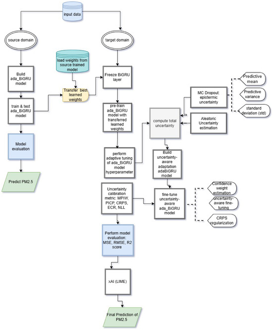
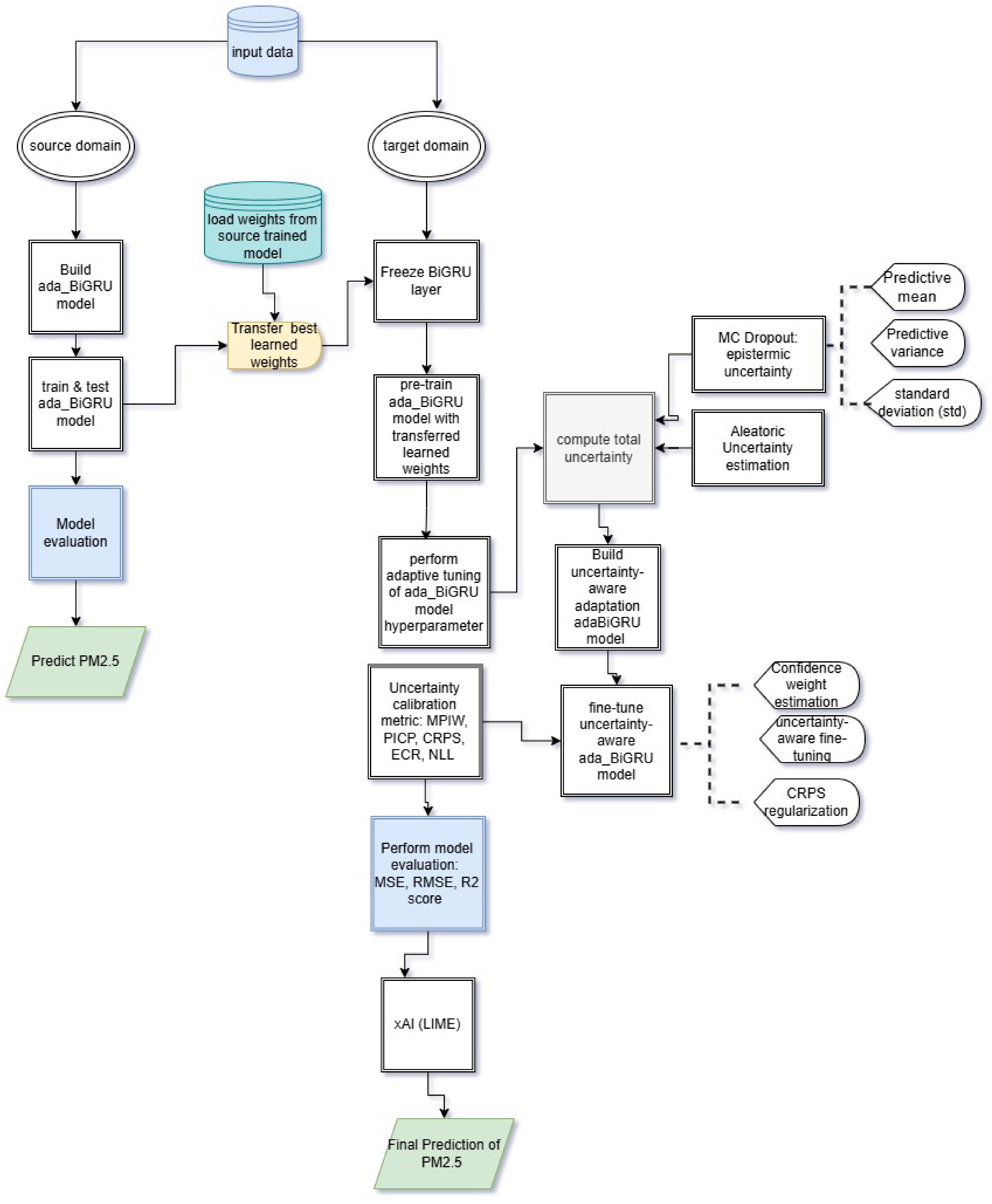
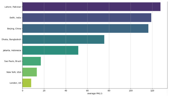
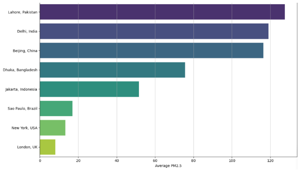
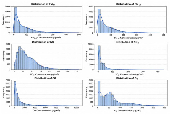
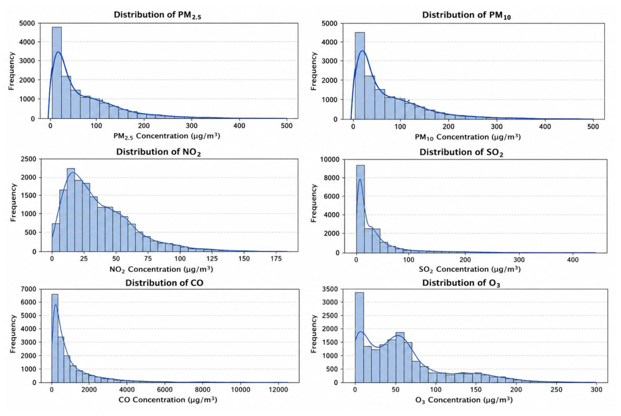
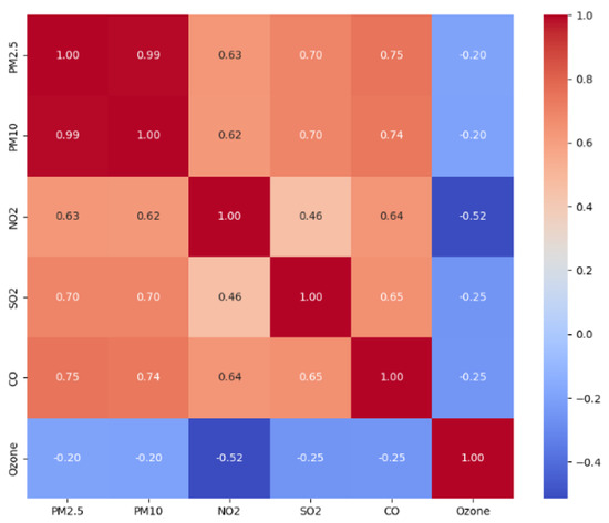
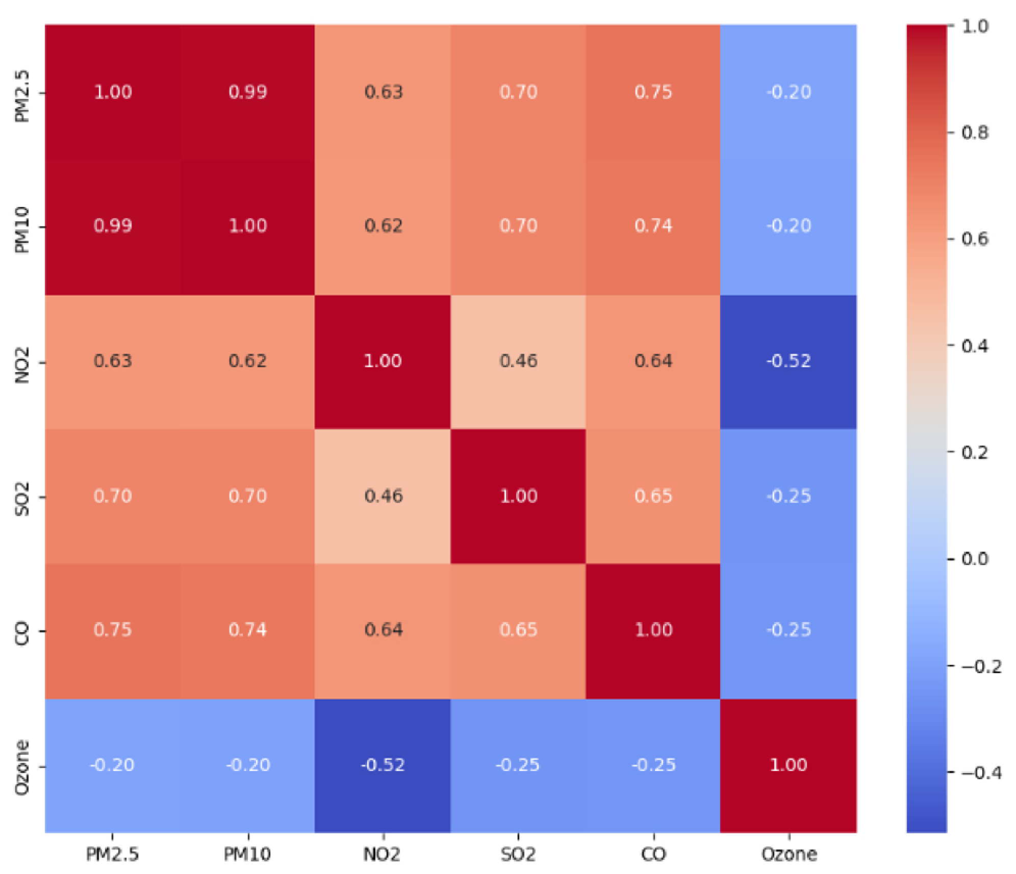
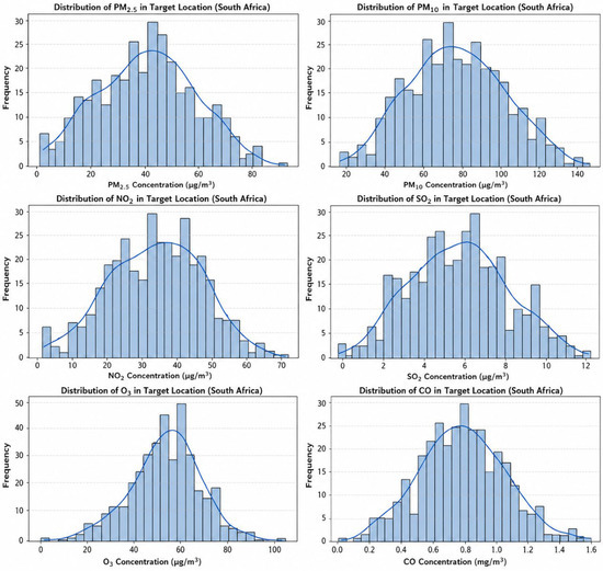
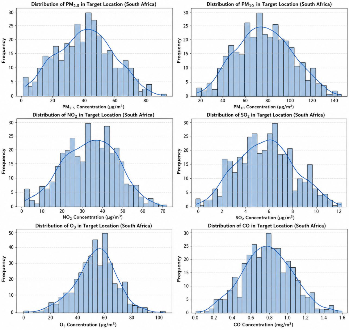
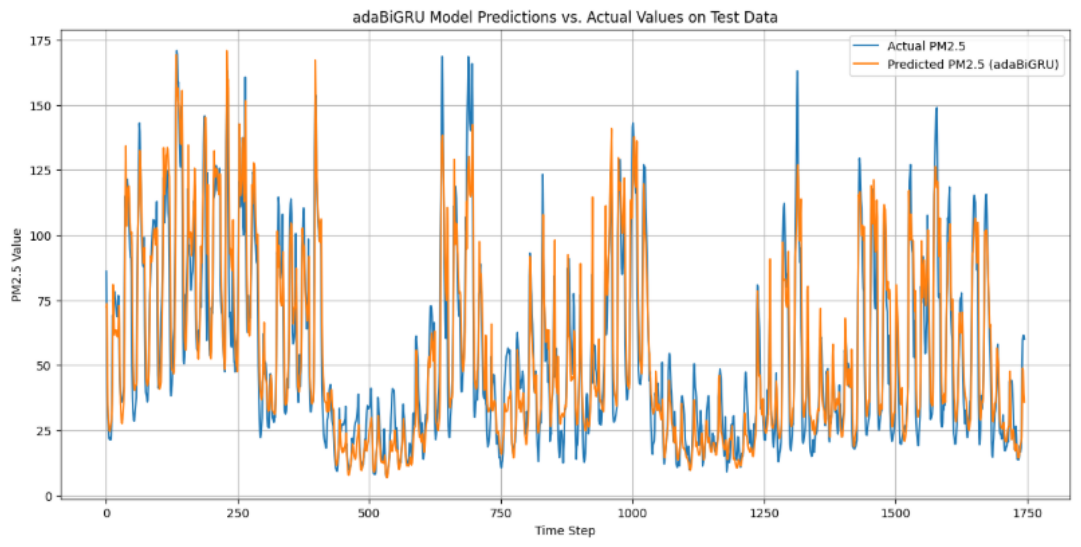
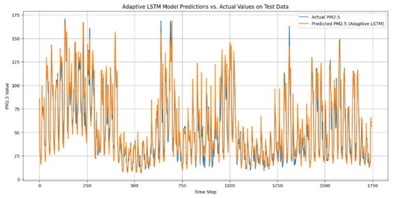
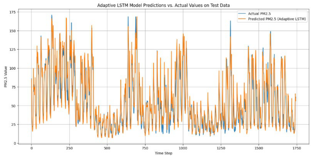
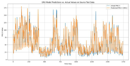
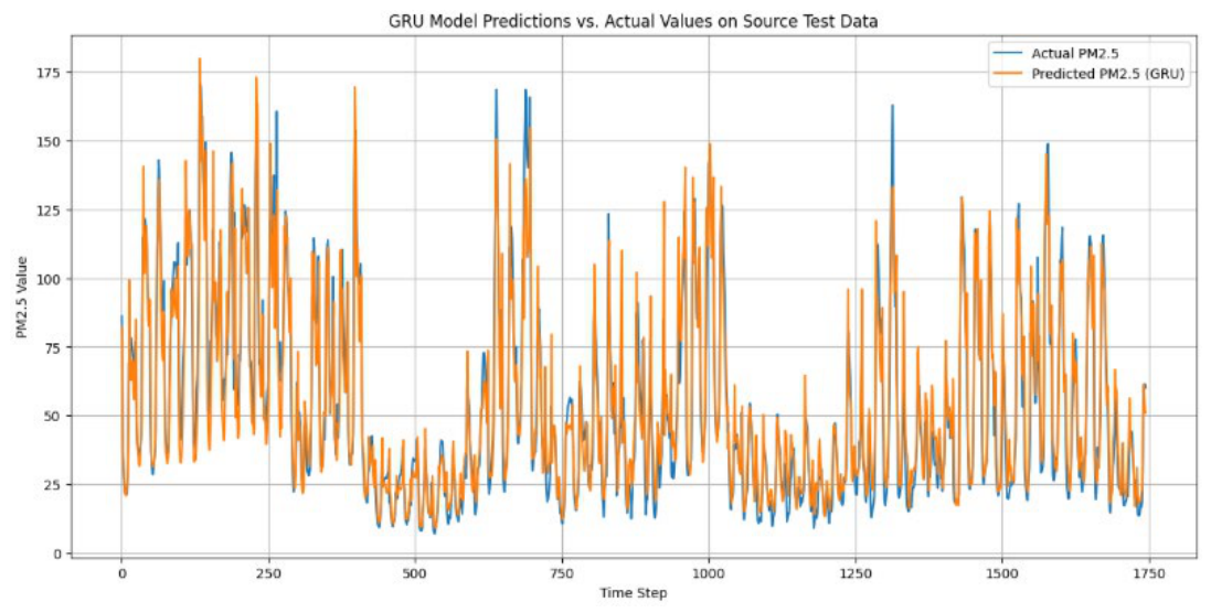
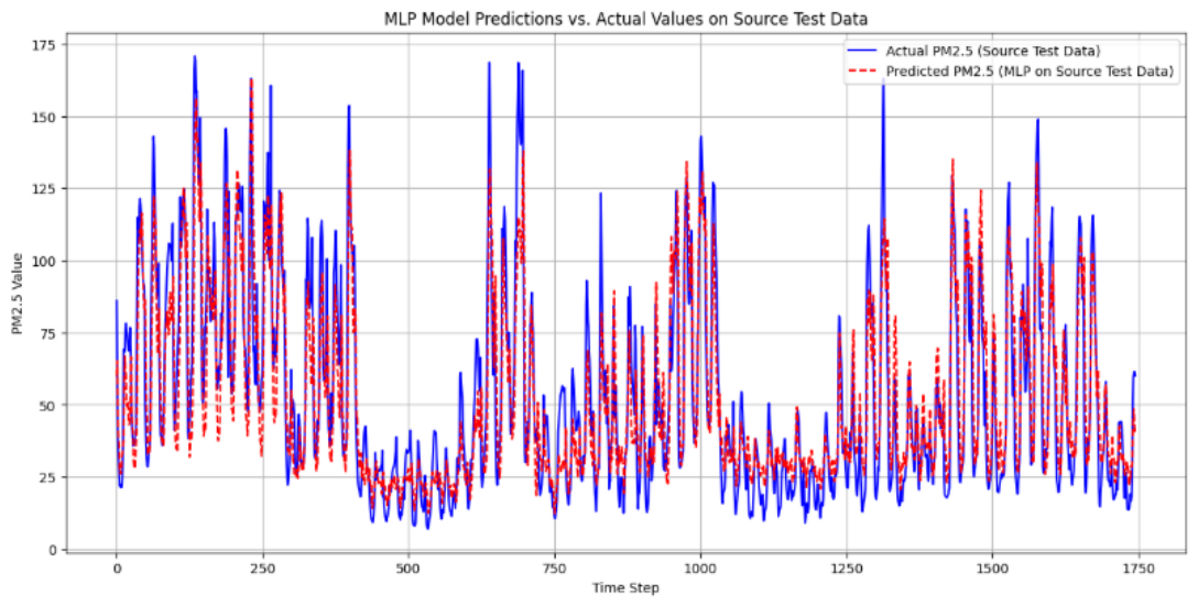
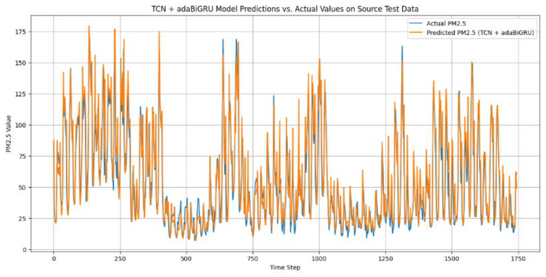
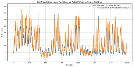
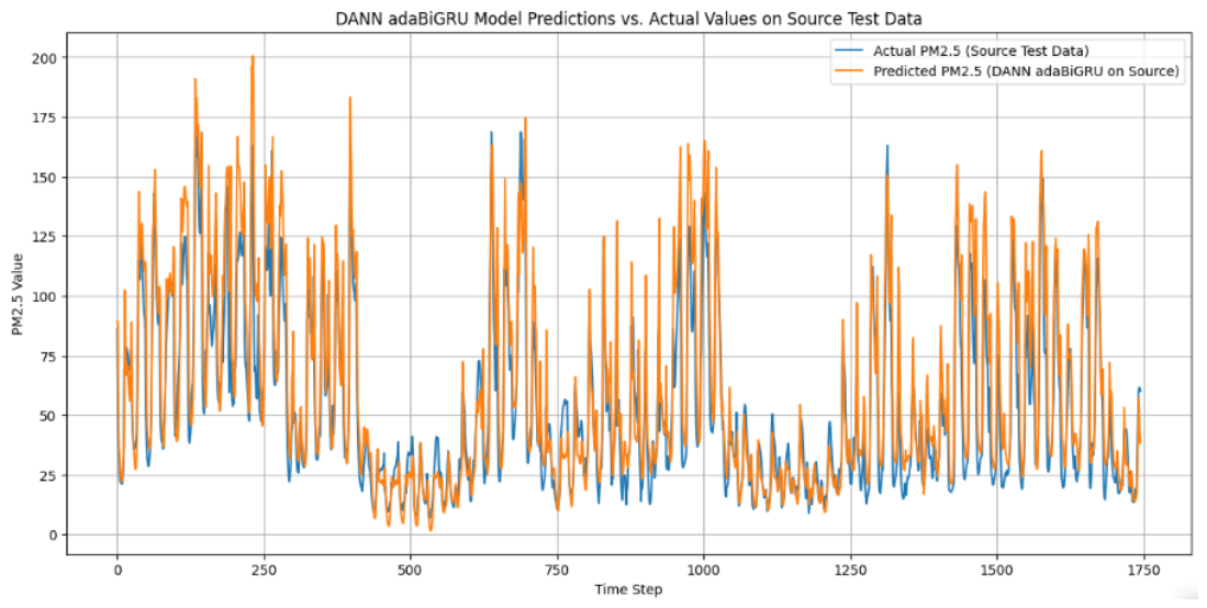
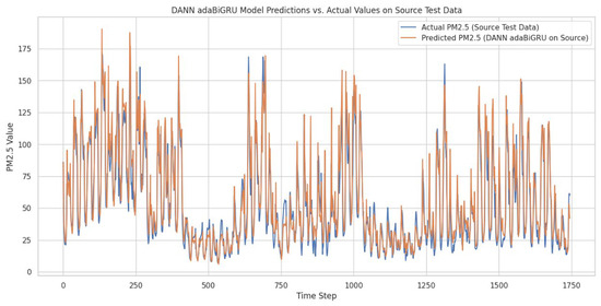
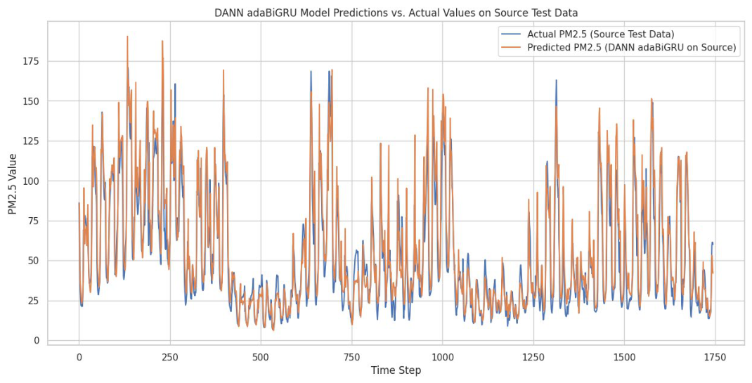
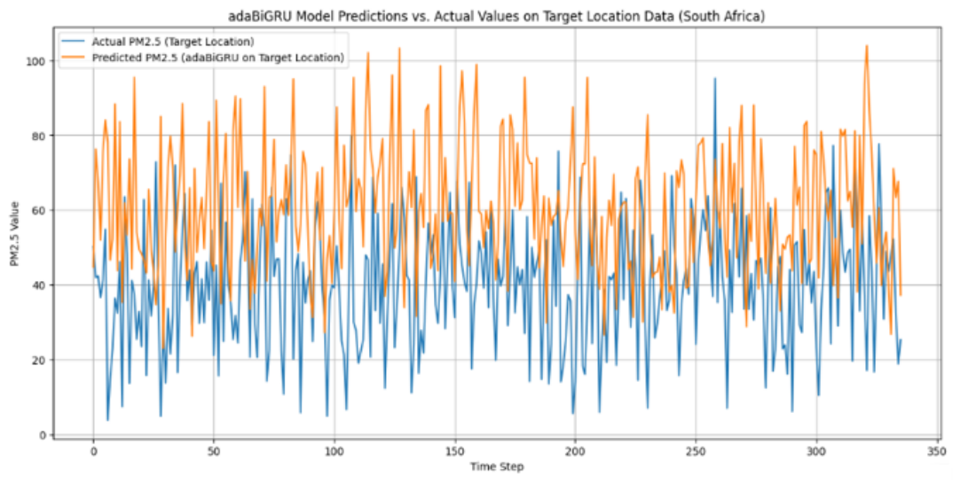
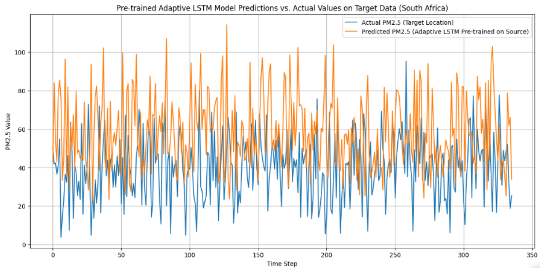
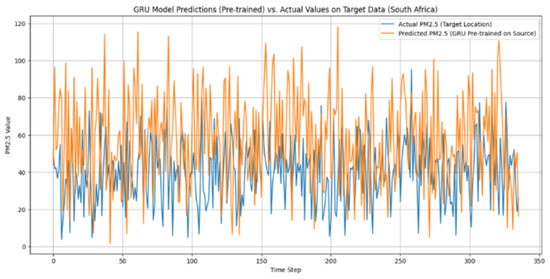
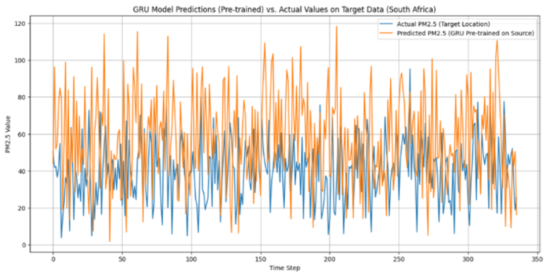
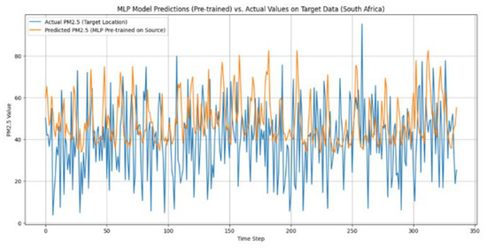
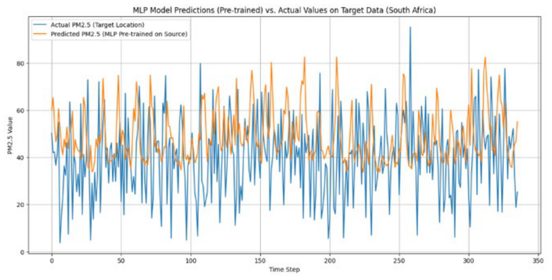
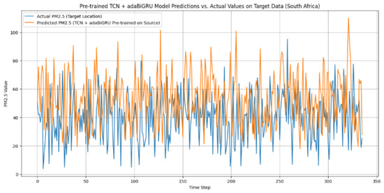
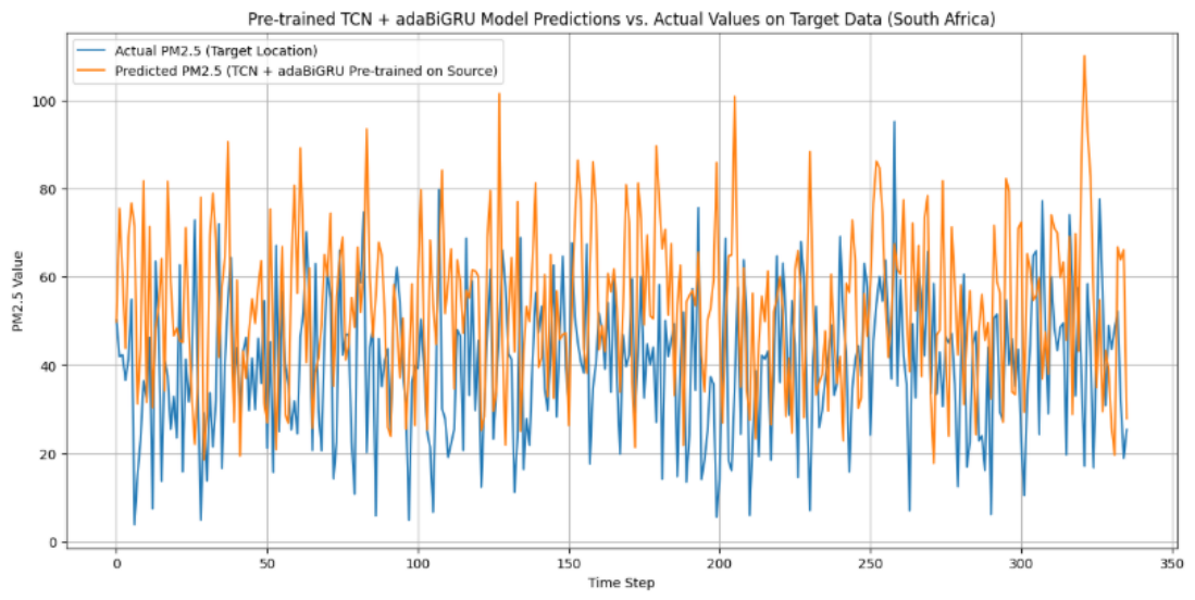
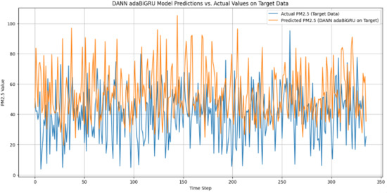
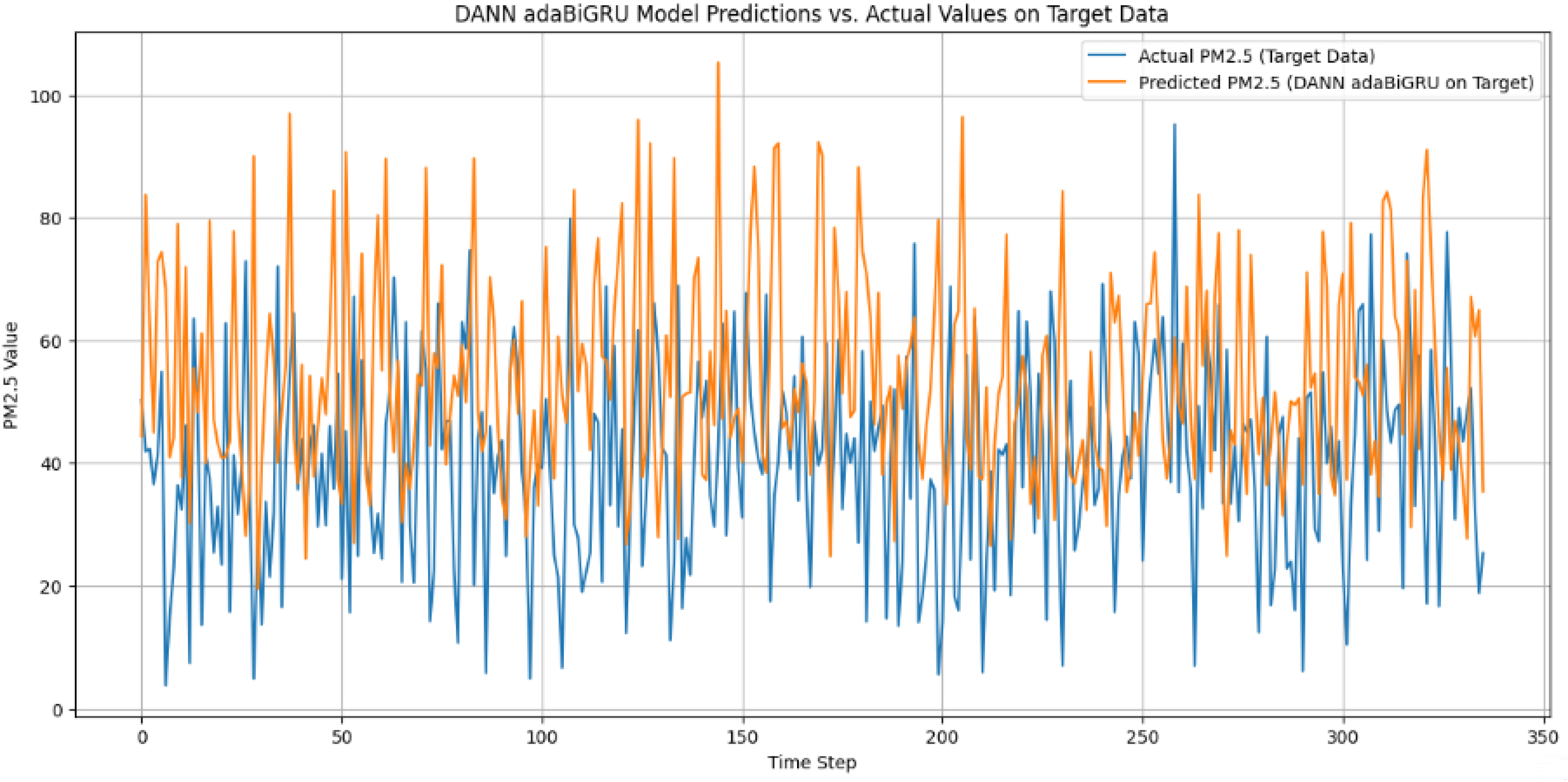
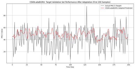
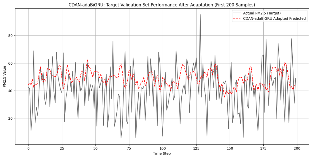
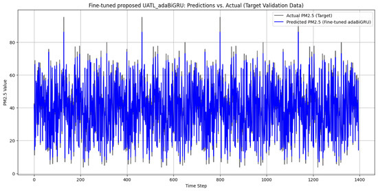
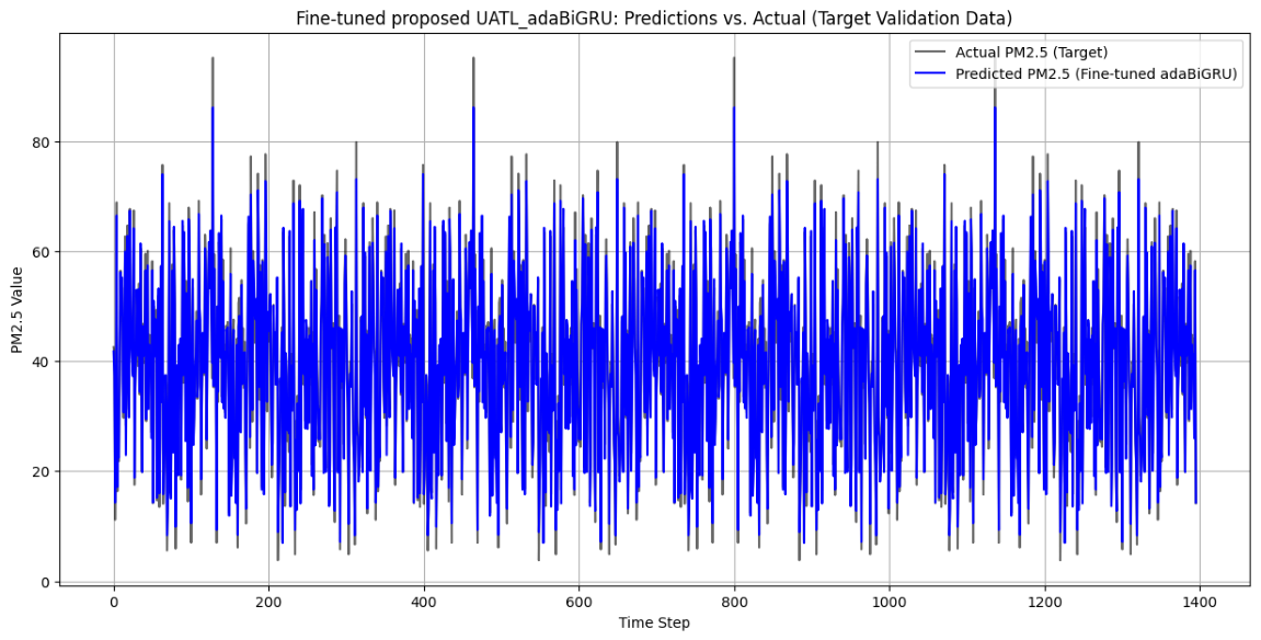
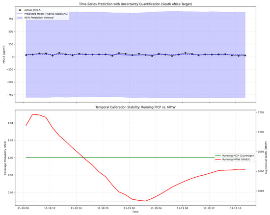
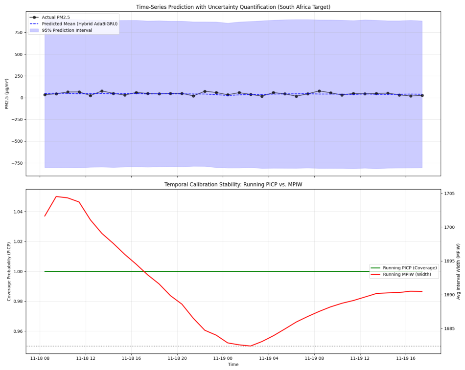
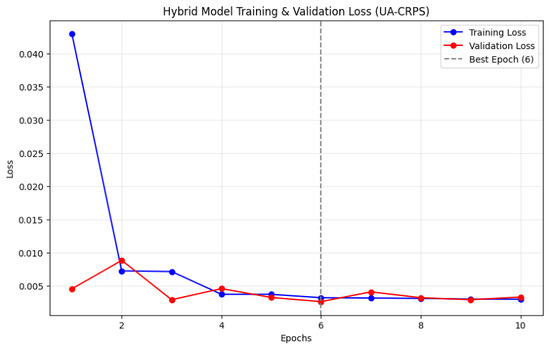
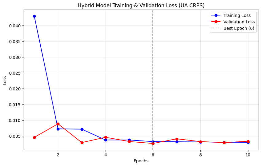
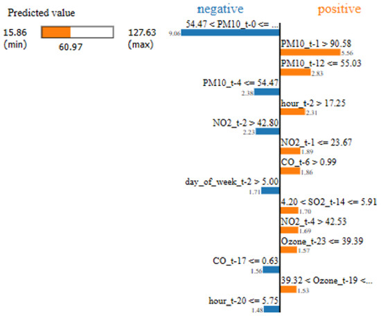
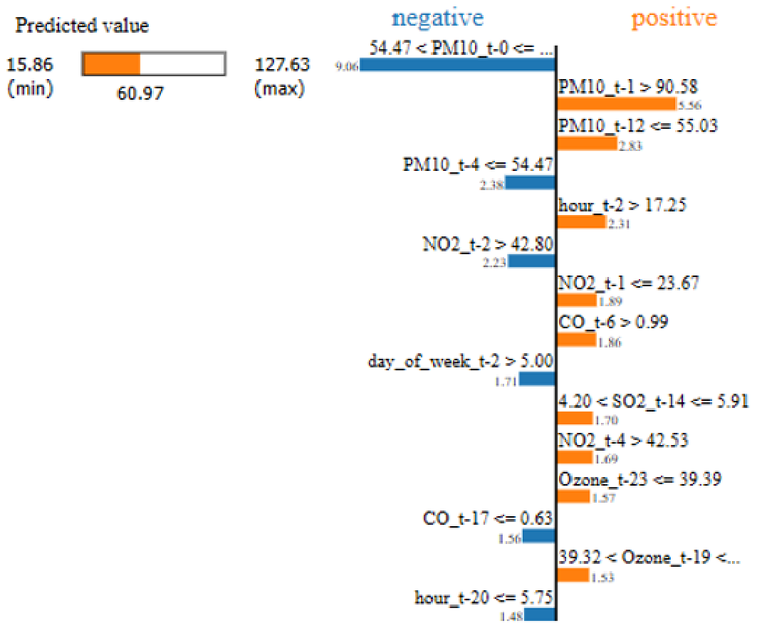
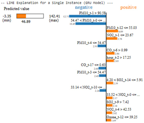
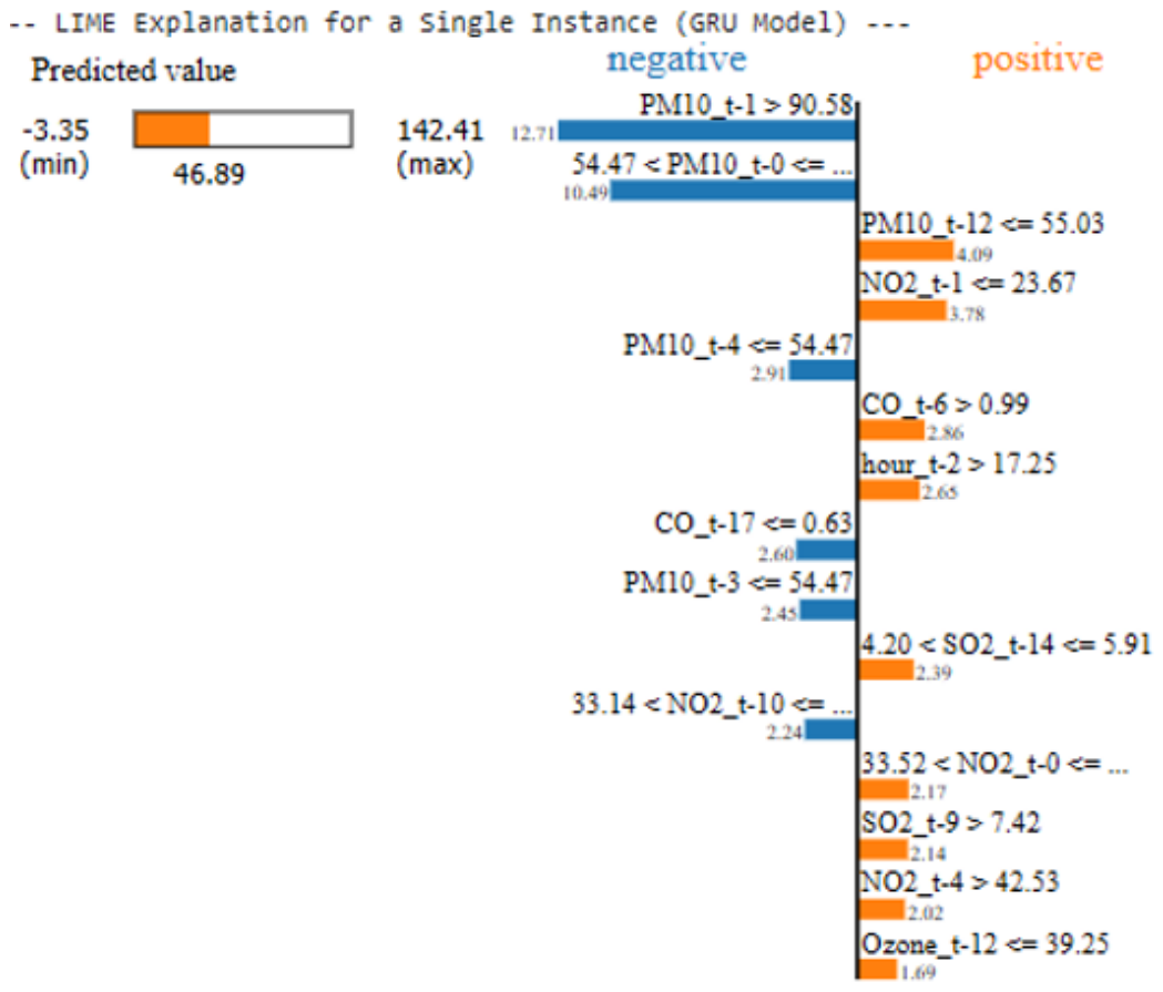
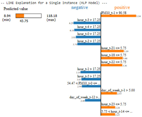
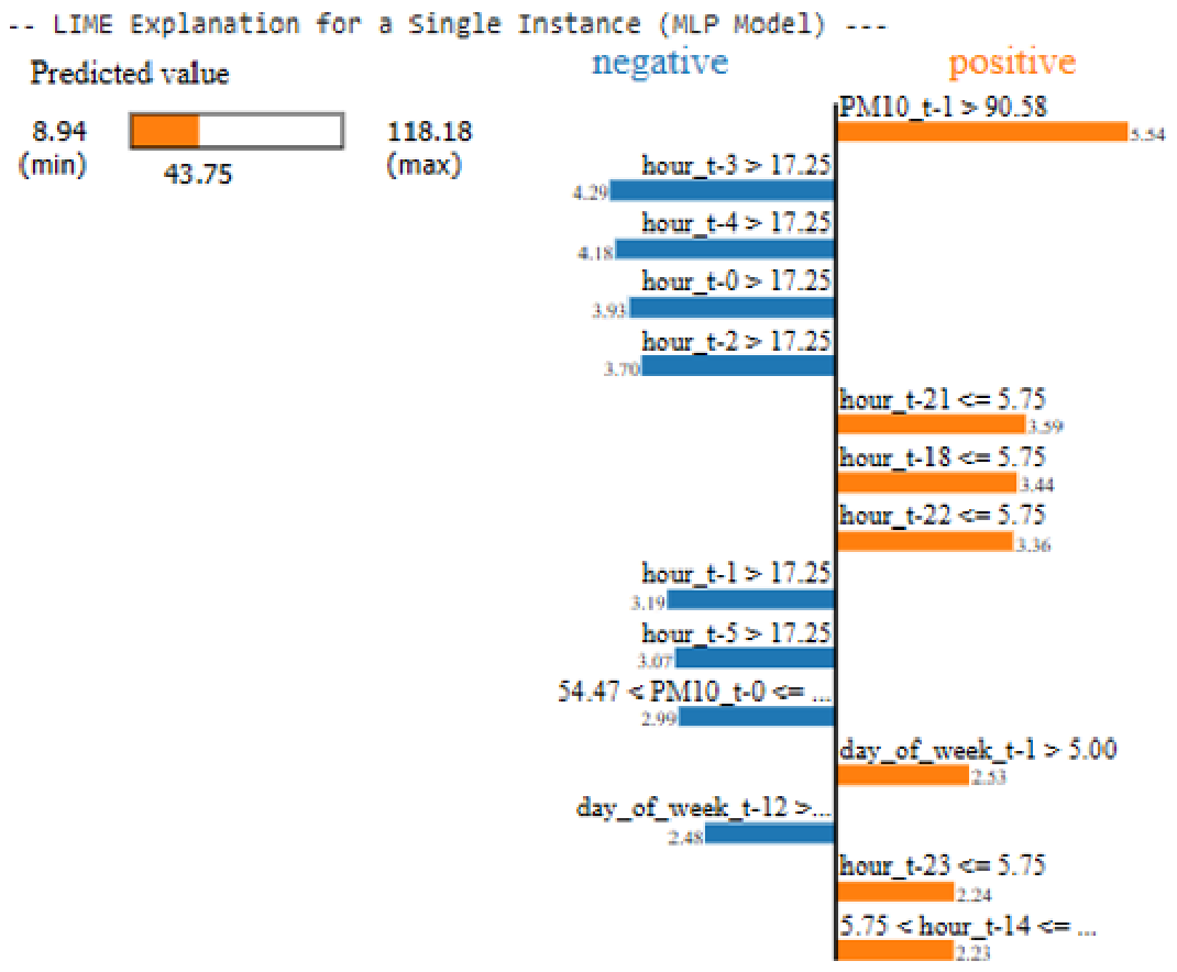
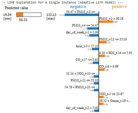
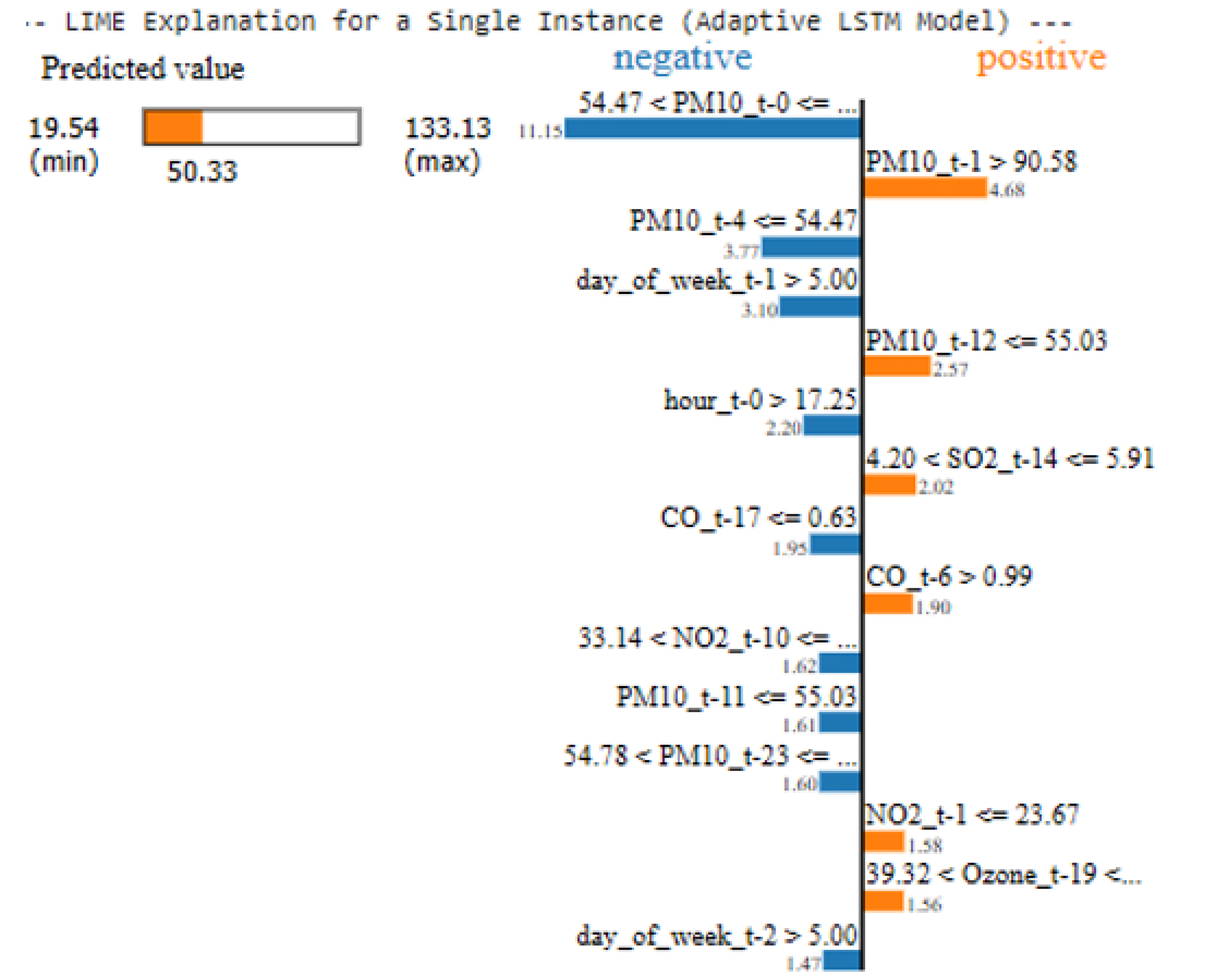
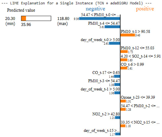
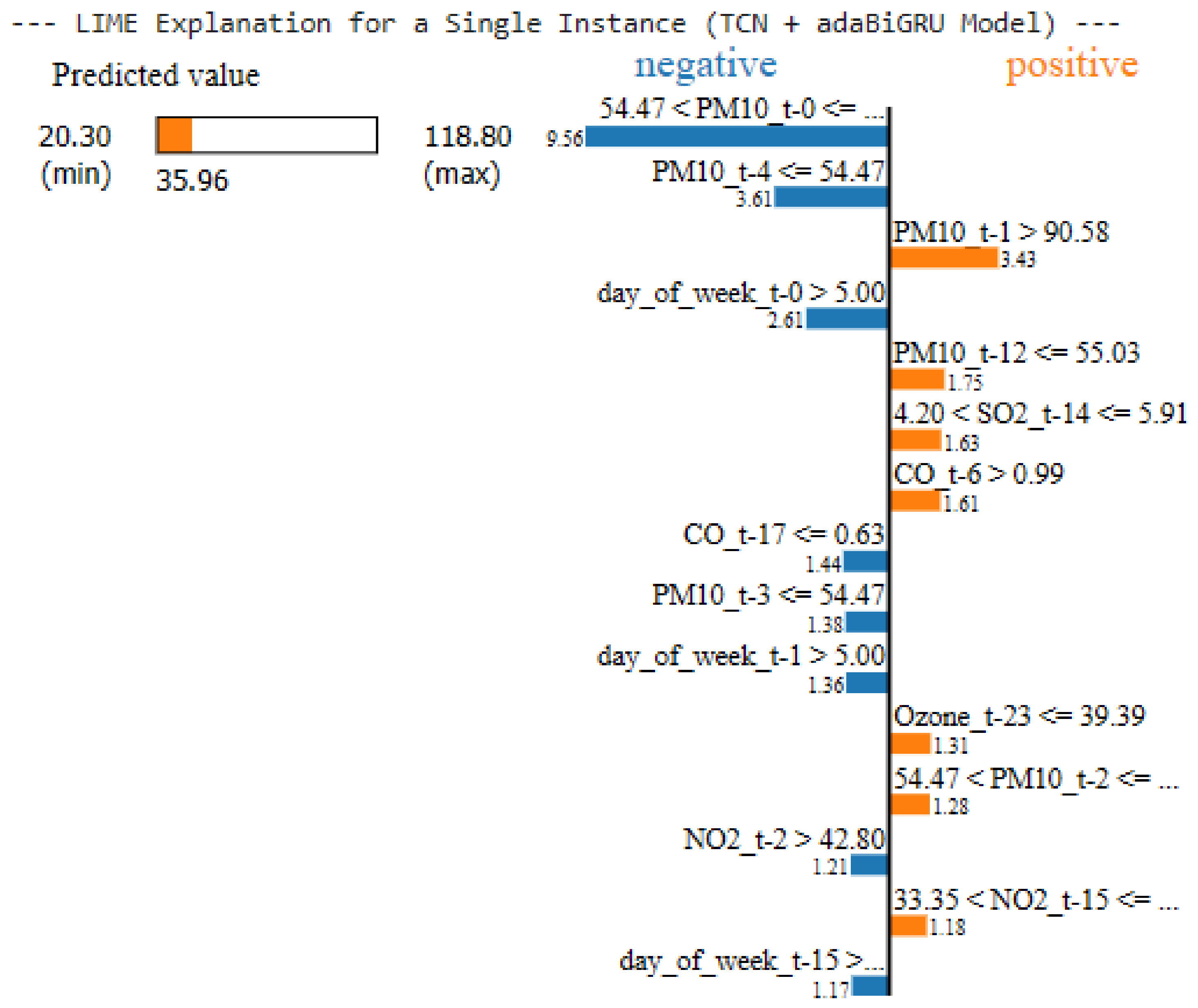
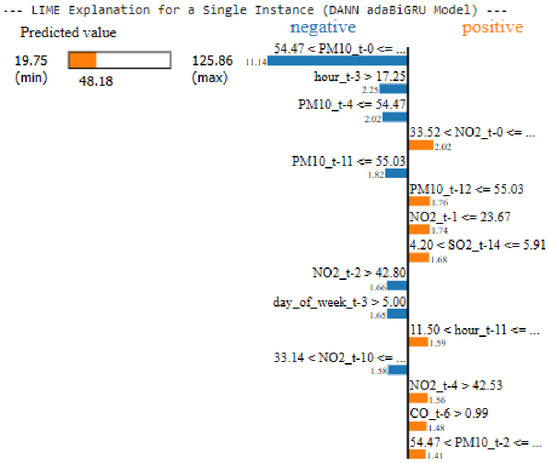
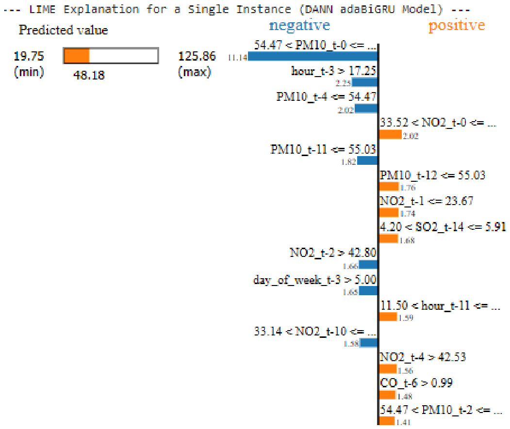
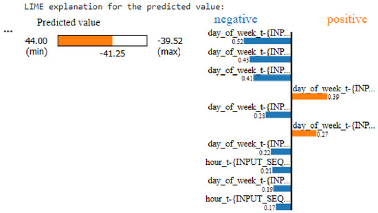
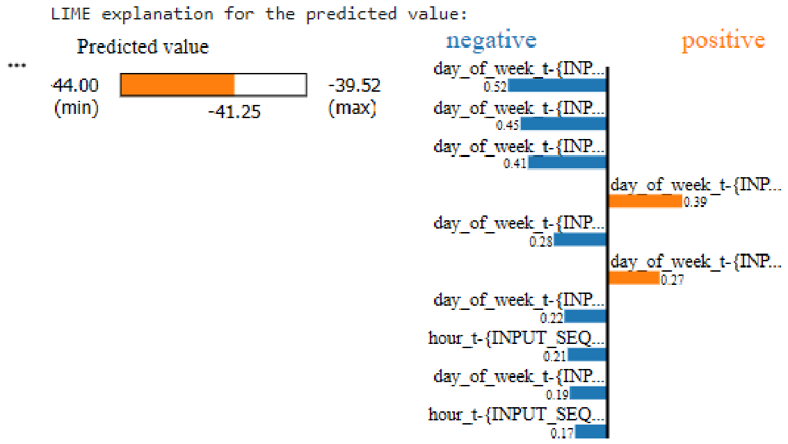
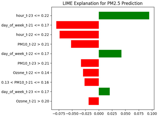
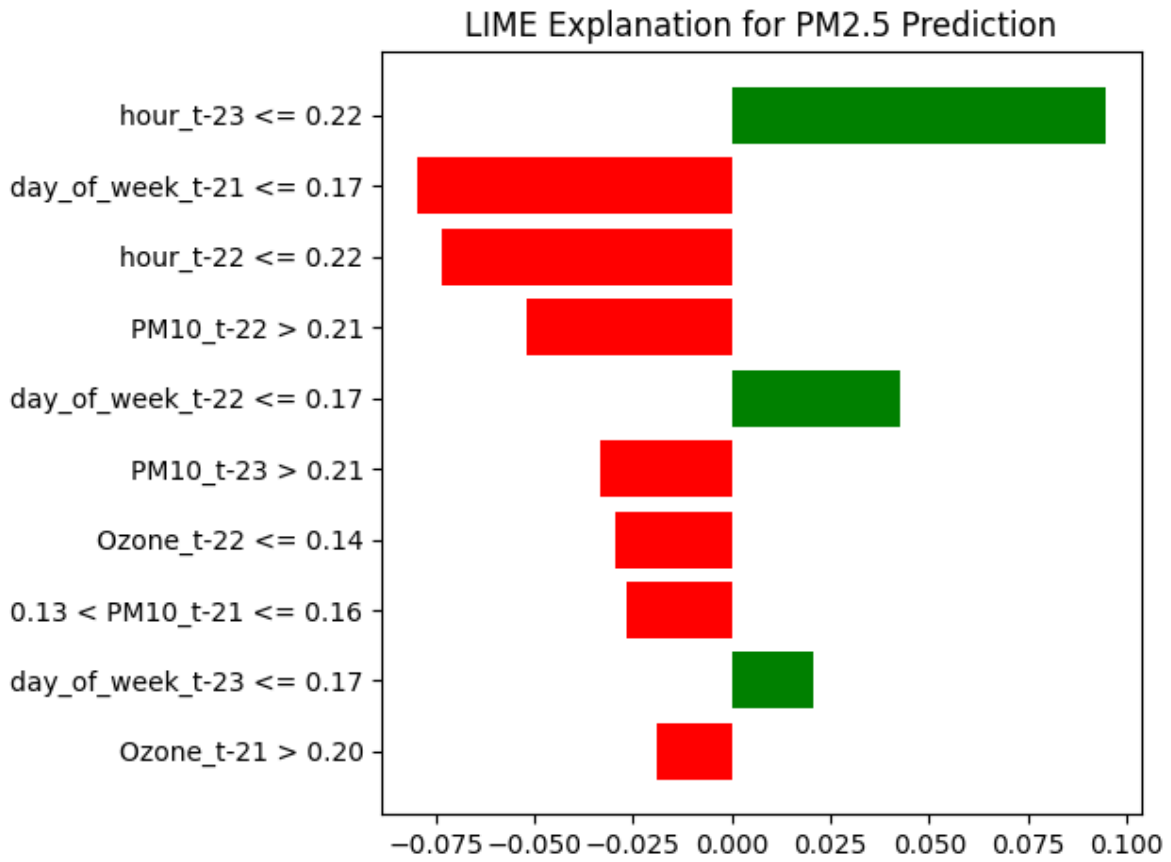

Disclaimer/Publisher’s Note: The statements, opinions and data contained in all publications are solely those of the individual author(s) and contributor(s) and not of MDPI and/or the editor(s). MDPI and/or the editor(s) disclaim responsibility for any injury to people or property resulting from any ideas, methods, instructions or products referred to in the content. |
© 2026 by the authors. Licensee MDPI, Basel, Switzerland. This article is an open access article distributed under the terms and conditions of the Creative Commons Attribution (CC BY) license.