


Highlights
What are the main findings?
- We introduce the generalized BPSARMA model, a new framework for modeling positive seasonal time series that allows the precision parameter to evolve dynamically over time.
- In several empirical applications involving reservoir inflow data, the proposed model often provides competitive or superior out-of-sample forecasting accuracy relative to alternative beta prime-based models, SARIMA, and Holt–Winters exponential smoothing.
What are the implications of the main findings?
- Allowing the precision parameter to vary over time provides a flexible way to capture changing variability in positive time series, potentially improving forecast performance.
- The proposed approach offers a practical forecasting tool for environmental and hydrological applications where the data are strictly positive and display seasonal patterns.
Abstract
This paper proposes a generalized seasonal beta prime autoregressive moving average model with dynamic precision, denoted by BPSARMA, for modeling and forecasting positive-valued seasonal time series. The proposed framework extends the generalized BPARMA model by incorporating stochastic seasonal dynamics in the conditional mean through seasonal autoregressive and moving average components while allowing a flexible autoregressive structure for the conditional precision parameter, thereby accommodating time-varying uncertainty. The model also allows the inclusion of covariates and deterministic seasonal regressors. Parameter estimation is carried out by conditional maximum likelihood, and the main inferential and diagnostic tools are discussed. Monte Carlo simulations are conducted to examine the finite-sample behavior of the estimators and associated inference procedures. The practical usefulness of the proposed approach is illustrated through hydro-environmental time series applications, where its forecasting performance is evaluated using both in-sample and out-of-sample predictive measures. The empirical results indicate that the BPSARMA specification often provides competitive or superior forecasting accuracy relative to competing models, highlighting its usefulness for modeling and prediction in positive seasonal time series.
1. Introduction
Time series assuming values on the positive real line arise naturally in many environmental and hydrological applications. Examples include river discharge, reservoir inflows, rainfall accumulation, pollutant concentrations, and wind speeds. Such variables typically display strong right-skewness and heteroscedastic behavior, with variability increasing with the level of the series. In addition, many environmental processes are subject to pronounced seasonal fluctuations driven by climatic cycles. These features often render classical Gaussian time series models inadequate for capturing both the distributional characteristics and the dynamic structure of the data.
In response to these challenges, increasing attention has been devoted to the development of observation-driven time series models based on non-Gaussian distributions defined on restricted domains. In particular, models built upon flexible continuous distributions supported on the positive real line have proven useful for describing environmental and hydrological processes. Such models offer an important practical advantage: they naturally produce forecasts that respect the support of the data, ensuring that predicted values remain in . Among the distributions suitable for this purpose, the beta prime distribution provides a versatile framework for modeling strictly positive data, as it accommodates a wide range of distributional shapes and allows the variance to vary with the mean in a natural way.
Dynamic models for time series taking values in have been extensively studied in the literature. The ARMA (beta autoregressive moving average) model for such series was introduced by [1] and later extended to accommodate time-varying precision by [2]. A modification of the model to incorporate stochastic seasonality while maintaining fixed precision was proposed by [3]. These models have been successfully applied to the modeling and forecasting of hydro-environmental time series; see, for instance, [4,5].
Recent advances in forecasting have also focused on nonlinear and regime-switching autoregressive structures, as well as Bayesian forecasting approaches. For example, Ref. [6] proposed a double-banded-threshold mixture autoregressive model for capturing complex nonlinear dynamics, while [7] developed Bayesian forecasting procedures for logistic mixture double autoregressive models with explanatory variables. These contributions highlight the growing interest in flexible forecasting frameworks capable of accommodating nonlinear behavior and time-varying dynamics. In contrast, the forecasting framework proposed in this paper is specifically designed for positive-valued seasonal time series and is based on a conditional beta prime distribution with dynamic mean and precision structures. The present contribution therefore complements these recent developments by addressing a different class of forecasting problems involving continuous positive-valued seasonal data.
The beta prime distribution, which is defined on the positive real line, is closely related to the beta distribution, arising as the distribution of the odds transformation of a beta random variable. This connection makes it a natural candidate for modeling positive-valued stochastic processes. In this paper, we develop a dynamic modeling framework based on the beta prime distribution, with particular emphasis on hydro-environmental time series exhibiting pronounced seasonal behavior.
The generalized BPARMA (beta prime autoregressive moving average) class of models for positive-valued time series, based on the beta prime distribution, was introduced by [8]. In that formulation, the conditional mean follows an autoregressive moving-average structure, while the precision parameter evolves dynamically through a first-order autoregressive specification. An important feature of this formulation is that both parameters of the conditional distribution evolve over time through separate dynamic submodels. As a result, temporal changes in the conditional density are governed not only by the mean but also by the precision parameter, allowing the model to capture time-varying variability in a flexible way. In the generalized BPARMA framework, seasonal patterns may be represented through deterministic regressors such as harmonic components and seasonal indicator variables.
Although this approach has proven useful in practice, many environmental time series exhibit seasonal dependence structures that are more complex than those captured by deterministic regressors alone. In particular, environmental processes often display seasonal dynamics that arise from stochastic dependence across seasons, in addition to deterministic periodic components. Moreover, the evolution of the variability of the series may require richer specifications for the precision parameter than a first-order autoregressive structure.
Motivated by these considerations, this article proposes an extension of the generalized BPARMA class that explicitly incorporates seasonal dynamics and a more flexible specification for the precision component. In the proposed model, the conditional mean follows a seasonal autoregressive moving-average structure in addition to the usual nonseasonal dynamics. At the same time, the precision parameter is allowed to follow an autoregressive process of general order, thereby expanding the range of dynamic heteroscedastic patterns that can be captured by the model. The resulting class, which we refer to as the BPSARMA model, also allows the inclusion of nonstochastic regressors, such as harmonic components and indicator variables, providing additional flexibility for representing deterministic seasonal patterns and structural changes.
Seasonality in environmental time series is often represented using one of several alternative approaches, such as seasonal dynamic components, harmonic regressors, or seasonal indicator variables. These strategies are frequently viewed as competing modeling choices. In practice, however, environmental processes may exhibit seasonal patterns that are too complex to be adequately represented by a single mechanism. In this article, we show that these approaches can be used jointly within a unified modeling framework. By extending the generalized BPARMA model to incorporate seasonal autoregressive and moving-average dynamics, the proposed specification allows deterministic seasonal regressors and stochastic seasonal dynamics to coexist in the same model. This combination proves particularly effective for the hydro-environmental series analyzed in this study, which exhibit strong and multifaceted seasonal fluctuations.
Parameter estimation is carried out by conditional maximum likelihood. Closed-form expressions are obtained for the conditional score vector and the conditional Fisher information matrix, facilitating numerical optimization and statistical inference. Diagnostic tools suitable for assessing model adequacy are also discussed. In addition, a Monte Carlo simulation study is conducted to examine the finite-sample performance of the proposed estimators.
The empirical usefulness of the proposed modeling framework is illustrated through five hydro-environmental applications involving monthly inflows to reservoirs associated with hydroelectric power plants located in the five geographic regions of Brazil. Brazil is a country of continental dimensions and is subject to diverse climatic regimes. Consequently, the analyzed series display substantial variability in their temporal behavior while sharing a common feature of strong seasonal fluctuations. Some series also present additional complexities, such as prolonged drought periods or structural changes in their level and variability. In our analysis, seasonal behavior is represented through a combination of three complementary mechanisms: seasonal dynamic components, harmonic regressors, and indicator variables. This strategy allows the model to capture both stochastic and deterministic aspects of seasonal variation.
The proposed model yields high-quality fits and accurate out-of-sample forecasts for all series considered. Its predictive performance is compared with that of several alternative approaches, including the BPSARMA model with fixed precision, the generalized BPARMA model, Gaussian SARIMA (seasonal autoregressive integrated moving average) models, and the Holt–Winters exponential smoothing algorithm. Overall, the results indicate that the proposed specification provides a flexible and effective framework for modeling positive-valued environmental time series exhibiting strong seasonal behavior and time-varying variability.
It is important to distinguish the present setting from the extensive literature on integer-valued time series, including threshold and count autoregressive models such as those developed by [9,10,11]. Those models are designed for discrete-valued count processes and rely on probabilistic mechanisms tailored to integer-valued data, such as thinning operators or count distributions. By contrast, the hydro-environmental series analyzed in this paper consist of continuous positive measurements. This distinction motivates the use of a beta prime conditional distribution together with dynamic structures for both the conditional mean and conditional precision.
The remainder of the paper is organized as follows: Section 2 introduces the proposed model and discusses its main properties. Section 3 presents the conditional maximum likelihood estimation procedure and derives the score vector and Fisher information matrix. Model selection, diagnostic tools, and forecasting are discussed in Section 4. Section 5 reports the results of the Monte Carlo simulation study. Section 6 presents the empirical applications to hydro-environmental time series. Finally, Section 7 concludes the paper.
2. A Seasonal Dynamic Extension of the Generalized BPARMA Model
In this section, we introduce the proposed seasonal dynamic extension of the generalized beta prime autoregressive moving average model. We begin with a brief review of the beta prime distribution and the generalized BPARMA framework of [8]. Building on this foundation, we develop a more flexible specification that incorporates stochastic seasonal dynamics in the conditional mean and allows for higher-order autoregressive structures in the precision submodel. These extensions broaden the range of temporal dependence patterns that can be captured within the beta prime time series framework.
2.1. The Beta Prime Distribution
The beta prime distribution was introduced by [12,13]. Also known as the inverse beta or beta type II distribution, it has support on the positive real line. The beta prime distribution arises as the distribution of the odds ratio associated with the beta distribution: if X follows a beta distribution, then follows a beta prime distribution. Equivalently, it can be expressed as the distribution of the ratio of two independent random variables following standard gamma distributions with unit scale parameter.
Later, Ref. [14] proposed a reparameterization in terms of a mean parameter and a precision parameter , which facilitates interpretation and makes the distribution particularly convenient for regression and time series modeling. Let Y be a random variable following a beta prime distribution, denoted by . The cumulative distribution function and probability density function are given, respectively, by
and
, where , denotes the regularized beta function,
is the incomplete beta function, and is the beta function, with denoting the gamma function. The mean and variance of Y are, respectively,
For all admissible values of and , the beta prime distribution is positively skewed. The skewness coefficient depends on both the mean and precision parameters and is given by
for . It is worth noting that in several traditional two-parameter distributions with support on the positive real line, the skewness coefficient depends only on the corresponding precision parameter, as is the case for the gamma distribution () and the reparameterized Birnbaum–Saunders distribution (). As discussed by [14], the beta prime distribution can exhibit substantially higher levels of skewness than those typically observed for the gamma and inverse Gaussian distributions.
2.2. The Generalized BPARMA Model
Ref. [8] introduced a dynamic model for variables taking values on the positive real line based on the beta prime distribution, referred to as the generalized BPARMA model. In this framework, the authors extended the classical formulation commonly adopted in dynamic models by incorporating a parsimonious dynamic submodel for the precision parameter. Specifically, an autoregressive and moving average structure was considered for the conditional mean, while a first-order autoregressive structure was specified for the conditional precision of the process. As a result, both parameters indexing the distribution evolve over time, providing greater modeling flexibility and allowing the conditional density to change shape throughout the time series.
Let be a time series of random variables such that, for , the conditional distribution of given the past information set , with denoting the -field generated by the information available up to time , is beta prime with mean and precision parameter , that is, . The conditional density of is
with . The conditional mean and conditional variance of are given by and , respectively.
The generalized model consists of two dynamic structures and is defined as
and
where and are scalar parameters, denotes an l-vector of nonstochastic regressors at time t, and is the corresponding vector of coefficients. The parameters correspond to autoregressive terms, while represent moving average parameters. The term denotes the random error on the predictor scale, and corresponds to the ratio between consecutive lagged observations. Moreover, denote the autoregressive and moving-average orders, respectively, with . The functions and are strictly monotonic and twice differentiable link functions, with inverses and also being twice differentiable.
When the series exhibits seasonal fluctuations, harmonic regressors are commonly used to represent periodic patterns. In this case, one may set , where S denotes the seasonal period. These regressors provide a parsimonious way of modeling deterministic seasonal cycles through sinusoidal functions, allowing the model to capture smooth periodic variations in the mean structure of the series. However, this specification assumes that the amplitude and phase of the seasonal pattern remain constant over time. This approach was employed in [8] in the analysis of water flow series from hydroelectric reservoirs.
2.3. The Generalized BPSARMA Model
We now introduce a seasonal dynamic extension of the generalized BPARMA model that increases its flexibility for modeling positive-valued time series. The proposed formulation incorporates stochastic seasonal autoregressive and moving average components in the conditional mean structure while allowing the precision parameter to follow an autoregressive process of arbitrary order. These features enable the model to capture evolving seasonal patterns and the evolution of the conditional precision.
The proposed generalized beta prime seasonal autoregressive moving average model, denoted by , is defined by
and
where B denotes the backshift operator such that, for a nonnegative integer b, . Furthermore, denotes the nonseasonal autoregressive polynomial, while corresponds to the nonseasonal moving average polynomial. The seasonal autoregressive polynomial is , whereas denotes the seasonal moving average polynomial. Here, . The seasonal period of the time series is represented by S and .
Although Equations (2) and (3) are defined for general link functions, throughout this paper, we employ the logarithmic link in both submodels, i.e., and . This choice is natural for positive-valued time series, since it ensures that both the conditional mean and the precision parameter remain positive. Furthermore, the transformation allows the dynamic dependence structure to be modeled on the log scale, where autoregressive and moving-average effects can be interpreted in terms of relative changes rather than absolute changes.
The regressors in the precision submodel are defined as relative increments of the response variable rather than as simple ratios of consecutive observations. This choice preserves the dimensionless nature of the precision covariates, which is important because the precision parameter must be free of measurement units. Indeed, since , a dimensionless ensures that the conditional variance has the appropriate squared measurement units of the response.
In addition, the adopted specification offers practical and interpretative advantages. First, the relative increment can be interpreted as a local growth rate, with zero indicating stability, positive values indicating increases, and negative values indicating decreases. This yields a more natural interpretation of the effect of recent changes on the precision dynamics. Second, unlike simple ratios, relative increments are centered around zero, which improves the interpretation of the intercept and may reduce collinearity with it. Finally, because precision is intended to capture changes in variability, using relative increments provides a more direct link between recent fluctuations in the series and the temporal evolution of the precision parameter. Preliminary empirical and simulation experiments with alternative ratio-based formulations consistently indicated better overall performance for the specification adopted here.
Equation (2) of the model can be written equivalently as
In what follows, we write , , , , and .
This representation makes explicit the dynamic specification adopted for the conditional mean on the transformed scale. In particular, it shows that evolves through a combination of nonseasonal and seasonal autoregressive components together with nonseasonal and seasonal moving-average terms. Expressing the model in this form clarifies its relationship with the generalized BPARMA structure while making the different dynamic contributions to the conditional mean more transparent. Moreover, it highlights how the proposed specification extends the original BPARMA framework by incorporating stochastic seasonal dynamics in the conditional mean while simultaneously allowing for richer temporal dependence in the precision submodel.
The dynamic structure specified for the conditional mean is similar to that adopted in the SARMA (beta seasonal autoregressive moving average) model and in the MKSARMAX (modified Kumaraswamy seasonal autoregressive moving average with exogenous regressors) model; see, respectively, [3,15]. It is important to emphasize, however, that those models were developed for random variables with support restricted to the unit interval. In contrast, the generalized BPSARMA model proposed in this paper is suitable for random variables defined on the positive real line.
An important feature of the proposed specification is that seasonal dynamics are modeled directly through seasonal autoregressive and moving average components. This approach allows seasonal patterns to evolve dynamically over time, rather than being restricted to fixed deterministic cycles. In many empirical applications, seasonality is introduced through harmonic regressors, which impose periodic patterns with constant amplitude and phase. While such representations are convenient, they assume that the seasonal structure remains stable throughout the sample.
In practice, however, seasonal patterns often evolve over time. This is particularly common in hydro-environmental time series, where seasonal fluctuations may change in magnitude, persistence, or timing due to climatic variability, hydrological regulation, or other environmental factors. Capturing these evolving seasonal dynamics is therefore important for an adequate statistical description of the data. The stochastic seasonal structure adopted in the proposed model accommodates such features by allowing the magnitude and persistence of seasonal effects to adjust according to the underlying dynamics of the process. As a result, the model provides a more flexible representation of seasonal behavior than approaches based solely on deterministic harmonic components.
It is also worth noting that the proposed formulation does not preclude the use of deterministic seasonal regressors. Because the model continues to allow the inclusion of covariates in the linear predictor through , harmonic regressors can be incorporated whenever appropriate. Consequently, the framework accommodates hybrid specifications that combine deterministic seasonal effects with stochastic seasonal dynamics.
In addition to incorporating a dynamic structure capable of capturing seasonality in the conditional mean submodel, the proposed model further generalizes the BPARMA formulation in the precision submodel; see Equation (3). The model introduced by [8] adopts a first-order autoregressive dynamic specification for the conditional precision. By contrast, in the formulation developed here, the precision submodel is specified through an autoregressive structure of order . This extension provides greater flexibility for modeling the temporal dynamics of the conditional precision, which reflects the level of uncertainty associated with the response variable.
Fluctuations in the precision parameter translate directly into changes in the conditional variance of the process. By allowing a higher-order autoregressive structure, the proposed specification allows the persistence and propagation of uncertainty levels to be captured more accurately over time. As a result, the model can accommodate richer patterns of temporal variation in conditional variability, yielding a more faithful representation of the evolving uncertainty underlying the observed series.
The model with fixed precision can be viewed as a particular case of the proposed formulation. It is obtained by adopting the identity link for and imposing , for . In this case, the precision parameter remains constant over time. This nested specification highlights that the proposed framework encompasses both time-varying and constant-precision models as special cases.
For ARMA models with fixed precision, consistency and asymptotic normality of the conditional maximum likelihood estimator can be established under conditions analogous to those used in Gaussian ARMA models, namely, requiring the autoregressive and moving-average polynomials to have no common roots and all roots to lie outside the unit circle; see [16]. However, such results do not directly extend to the present generalized BPSARMA formulation, which combines stochastic seasonal components, dynamic precision governed by a higher-order autoregressive structure, and nonlinear link functions in both submodels. In particular, the interaction between seasonal and nonseasonal autoregressive polynomials and the simultaneous evolution of preclude a direct application of the root-restriction arguments used in the simpler setting.
Because the generalized BPSARMA model is specified through conditional mean and precision recursions, inference and forecasting are developed conditionally on the past information set . The usual notion of stationarity retains its conventional meaning as a property of the unconditional joint distribution of the process; however, since the estimation framework is entirely conditional and no analytical characterization of the admissible parameter space is currently available for this model class, stationarity is not operationally enforced during estimation. Instead, numerical stability of the conditional recursions serves as the relevant practical criterion.
No explicit stationarity or invertibility constraints are therefore imposed during the numerical maximization of the conditional log-likelihood. As a pragmatic diagnostic strategy, similarly to [17], autoregressive or moving-average parameter estimates with unusually large magnitudes (particularly exceeding one in absolute value) may be regarded as potential indicators of numerical instability in the conditional recursions for . In the empirical applications presented in this paper, no such signs of instability were detected. We emphasize, however, that this is only an ad hoc diagnostic criterion: unstable behavior in the recursions may still arise even when all estimated coefficients lie within , and, conversely, estimates outside this range do not necessarily imply divergence of the fitted process. As in the related GARMA and dynamic beta regression literature, inference and forecasting are grounded in the conditional specification of the model.
3. Conditional Likelihood Inference
Let denote a realization from a stochastic process, and let denote the w-dimensional parameter vector, where . Let , which represents the minimum number of initial observations required for the conditional likelihood evaluation. The conditional log-likelihood function can be written as
where
We now derive the conditional score vector and the conditional Fisher information matrix, obtained from the first- and second-order derivatives of Equation (4), respectively. To this end, we partition the parameter vector as , where
As before, we consider the error defined on the predictor scale. In what follows, primes denote derivatives.
3.1. Conditional Score Vector
The conditional score vector is obtained from the first-order derivatives of the conditional log-likelihood function given in Equation (4) with respect to the components of the parameter vector .
Let and denote the vectors of partial scores associated with the mean and precision submodels, respectively. We also define the diagonal matrices and , as well as the vectors and . Additionally, let , , , , and be matrices of dimensions , , , , and , respectively, with corresponding elements
The score vector is given by
with components
where denotes an vector of ones. Further details are provided in Appendix A.
The conditional maximum likelihood estimator (CMLE) of , denoted by , is obtained as the solution of the nonlinear system of equations , where denotes a null vector of dimension w. However, this system does not admit a closed-form solution. Consequently, the CMLEs are obtained through iterative computational procedures based on the maximization of the conditional log-likelihood function using Newton or quasi-Newton nonlinear optimization algorithms. For further details, see [18,19].
To implement the iterative procedure, initial values for and must be specified. For , the quantities and are computed using the derivatives with respect to the parameters of the mean and precision submodels, respectively.
3.2. Conditional Information Matrix
To obtain the conditional Fisher information matrix, , it is necessary to compute the second-order derivatives of the conditional log-likelihood given in Equation (4) and their expected values. These results allow the computation of the standard errors of the CMLEs, the construction of asymptotic confidence intervals, and the implementation of hypothesis tests. The matrix corresponds to the conditional Fisher information matrix, obtained as the expectation of the negative Hessian of the conditional log-likelihood.
Let , and . The conditional Fisher information matrix associated with the parameter vector can be expressed as
where , , , , , , , , , , , , , , , , , , , , , , , , , , , , , , , , , , and . For details, see Appendix A.
Under the usual regularity conditions and for sufficiently large n, the CMLE is consistent and asymptotically normally distributed [20]. In particular,
approximately, where denotes the w-dimensional normal distribution, and is the CMLE of .
3.3. Confidence Intervals and Hypothesis Testing
Let denote the s-th component of the parameter vector , the corresponding conditional maximum likelihood estimator contained in , and the s-th element of the main diagonal of the inverse Fisher information matrix evaluated at , for . From the asymptotic normality of the CMLE of , it follows that
approximately. This result can be used to construct asymptotic confidence intervals as well as to perform hypothesis tests on the model parameters.
An asymptotic confidence interval for , with confidence level , , is given by
where denotes the quantile of the standard normal distribution. For further details on asymptotic confidence intervals, see [21].
The asymptotic normality of can also be used to perform hypothesis tests on the parameters indexing the model. Suppose we wish to test against . The z test statistic is given by
Under and for sufficiently large n, z is approximately standard normally distributed. Thus, for a given significance level , is rejected if .
When the interest lies in simultaneously testing multiple parametric restrictions, more general hypothesis tests may be employed, such as the likelihood ratio test [22], the score test [23], and the Wald test [24]. Under and for sufficiently large samples, the statistics associated with these tests are asymptotically -distributed, with degrees of freedom equal to the number of imposed restrictions.
4. Model Selection, Diagnostic Analysis, and Forecasting
In this section, we present the model selection criteria, diagnostic tools, and forecasting procedures adopted for the generalized BPSARMA model. The diagnostic analysis aims to assess whether the fitted model adequately captures the dynamic structure present in the data. If this condition is satisfied, the model can be regarded as suitable for producing reliable out-of-sample forecasts.
4.1. Model Selection
Information criteria are widely used in model selection, particularly when comparing competing specifications within the same model class. For selecting the generalized BPSARMA model, we adopt the modified Bayesian information criterion (MBIC) proposed by [3]. This modified criterion is defined as
where denotes the maximized value of the log-likelihood function. The authors also considered a modified version of the Akaike Information Criterion (MAIC).
4.2. Residuals
Residual analysis constitutes a fundamental step in assessing the adequacy of the estimated model to the observed data. To investigate the fit of the generalized BPSARMA model, we employ the quantile residual, which is widely used in the literature on regression and time series models. This residual is defined as
where denotes the cumulative distribution function of the standard normal distribution and its corresponding quantile function, and represents the conditional cumulative distribution function of the beta prime distribution, conditional on the past information set , evaluated at . Under correct model specification, the quantile residual is asymptotically standard normally distributed [25].
4.3. Portmanteau Tests
Portmanteau-type tests are widely used to assess the adequacy of a fitted model. This assessment is based on jointly verifying whether the first v autocorrelations of the residuals equal zero; that is, the null hypothesis is tested. One of the most commonly used test statistics is the one proposed by [26]. An alternative is the statistic proposed by [27], which is based on the partial autocorrelations of the residuals.
The model is considered adequate if the residual autocorrelations (or partial autocorrelations) do not jointly differ significantly from zero. Otherwise, the fitted specification may be regarded as inadequate, and the fitted model is rejected. Under the null hypothesis, these statistics are asymptotically -distributed with degrees of freedom. Ref. [3] suggests adopting .
4.4. Forecasting
In-sample forecasts for the conditional mean of , with , are given by the fitted conditional means . These forecasts are constructed by setting for and, for , taking . Additionally, the unknown parameters in Equation (2) are replaced by their conditional maximum likelihood estimates, after which the inverse link function is applied. Thus, the in-sample forecast , for , is given by
Similarly, out-of-sample forecasts can also be obtained. The h-step-ahead forecast of the conditional mean, for , is denoted by and is given by
where
5. Simulation Results
In this section, we present Monte Carlo simulation evidence on the finite-sample properties of the CMLEs of the parameters indexing the model. We consider four sample sizes, namely . In each replication, a burn-in period of length 1000 was used; that is, time series of length were generated, and the first 1000 observations were discarded in order to mitigate the influence of initial conditions on the simulated sample paths. The resulting series are denoted by . Each series was generated from the generalized BPSARMA model specified in (2) and (3), using the logarithmic link function in both submodels.
Parameter estimation was performed by numerically maximizing the conditional log-likelihood function. For this purpose, we employed the quasi-Newton limited-memory Broyden–Fletcher–Goldfarb–Shanno algorithm with box constraints (L-BFGS-B), using analytical first derivatives. The initial parameter values were specified as follows: the initial values for , , and were obtained from ordinary least squares estimates of the linear regression of on and , and in this case, the initial value of corresponds to the intercept of the regression; the parameters , and were initialized at zero; the initial value of was obtained as
where is the sample variance of ; and, finally, the coefficients of the precision submodel, , were initialized at , providing simple feasible starting values for the numerical optimization.
The initialization strategy was designed to provide starting values that are consistent with the dynamic structure of the model while maintaining numerical stability during optimization. In particular, the initial values of , , and were obtained from a linear approximation to the conditional mean dynamics on the link-function scale. The moving-average parameters were initialized at zero, a common choice in likelihood-based estimation of ARMA-type models, since reliable preliminary estimates of these parameters are generally unavailable. The initial value of was obtained by matching the sample moments to the variance structure implied by the beta prime distribution. The coefficients of the precision submodel were initialized at , providing a simple and feasible starting configuration while allowing for an initial negative association between recent relative changes in the series and the precision dynamics, which is often observed in preliminary empirical analyses. Alternative initialization strategies, including different fixed starting values for the moving-average parameters and for the coefficients of the precision submodel, were also explored in preliminary numerical experiments. The adopted scheme was retained because it consistently yielded stable convergence and satisfactory optimization performance while remaining computationally simple.
The simulations were carried out using the statistical computing environment [28]. A total of 5000 Monte Carlo replications were conducted, and no convergence failures occurred during the numerical maximization of the log-likelihood function. We adopt the logarithmic link function for both the mean and precision submodels.
In the first simulation scenario, the data were generated from the model. The parameter values were set to , , , , , , , and . These values correspond to the point estimates obtained from fitting the model to real data on inflow to the Estreito reservoir and therefore represent a realistic empirical configuration.
Table 1 reports, for each estimator, the estimated mean (Mean), standard deviation (SD), bias (Bias), and mean squared error (MSE). As expected, both the biases and the mean squared errors decrease as the sample size increases, providing evidence of the consistency of the CMLEs. It is also observed that the parameters , , , and tend to be underestimated. This behavior is consistent with the results reported for the SARMA model in [3].
Table 1.
Monte Carlo results for the CMLEs under the model: mean (Mean), standard deviation (SD), bias (Bias), and mean squared error (MSE); first scenario.
The tendency toward negative bias in the estimators of , , , and is likely a finite-sample effect associated with the estimation of dynamic dependence parameters in ARMA-type models. Similar behavior has been reported for the SARMA model by [3]. The effect is particularly pronounced for the seasonal parameters, whose estimation relies on observations separated by one seasonal cycle. Consequently, the effective amount of information available for estimating and is smaller than that available for the corresponding nonseasonal parameters, leading to larger finite-sample biases. As expected, these biases decrease steadily as the sample size increases.
In addition, the biases of the estimators of the nonseasonal parameters, and , decrease more rapidly than those of the seasonal parameters, and . This finding corroborates the discussion in [29], according to which the estimators of seasonal parameters tend to exhibit larger biases than the remaining estimators. For example, when , the estimated bias of () is (), whereas that of () is (). Overall, the results indicate that the parameters of the generalized BPSARMA model can be estimated with good accuracy, particularly as the sample size increases.
A different pattern is observed for the intercept parameter , whose estimator exhibits a comparatively larger finite-sample bias. This behavior may be attributed, at least in part, to the fact that the intercept is estimated jointly with the autoregressive, moving-average, seasonal, and precision components and therefore reflects the cumulative effect of finite-sample estimation errors in the remaining parameters. Nevertheless, the bias decreases rapidly as the sample size increases, falling from when to when , which provides further evidence of the consistency of the CMLE.
We next present four additional simulation scenarios aimed at evaluating the finite-sample performance of inference for the parameters indexing the proposed model. For these additional scenarios, we considered only the sample sizes . These sample sizes were selected to represent moderate- and large-sample settings, allowing us to evaluate the rate at which the asymptotic properties of the estimators become evident. In addition to the point-estimation results, we report the empirical coverage rates (CRs) of the asymptotic confidence intervals. The adopted specification is the model, under different combinations of the parameter values and , allowing us to investigate distinct levels of seasonal dependence as well as different dynamic regimes in the variable-precision component. Specifically, the parameter values were set to , , , , , , and .
The results for the four additional simulation scenarios are reported in Table 2, Table 3, Table 4 and Table 5. Overall, the point estimators display satisfactory finite-sample performance. In general, the means of the estimates remain close to the corresponding true parameter values, even for the smaller sample size (), indicating relatively small biases. Moreover, these biases systematically decrease as the sample size increases. A substantial reduction in the standard deviations is also observed as n increases. For nearly all parameters, the variability of the estimators when is less than half of that observed for , reflecting considerable gains in precision. Consequently, the mean squared errors decrease markedly across the sample sizes. Taken together, these results indicate that increasing the amount of sample information contributes simultaneously to reducing both bias and variability, which is consistent with the asymptotic behavior expected for the CMLEs and provides favorable empirical support for their use in moderate and large samples.
Table 2.
Monte Carlo results for the CMLEs under the model: mean (Mean), standard deviation (SD), bias (Bias), mean squared error (MSE), and coverage rate (CR); second scenario.
Table 3.
Monte Carlo results for the CMLEs under the model: mean (Mean), standard deviation (SD), bias (Bias), mean squared error (MSE), and coverage rate (CR); third scenario.
Table 4.
Monte Carlo results for the CMLEs under the model: mean (Mean), standard deviation (SD), bias (Bias), mean squared error (MSE), and coverage rate (CR); fourth scenario.
Table 5.
Monte Carlo results for the CMLEs under the model: mean (Mean), standard deviation (SD), bias (Bias), mean squared error (MSE) and coverage rate (CR); fifth scenario.
A comparison across the different simulation scenarios reveals that the estimators of the parameters associated with the precision dynamics ( and ) generally exhibit the largest standard deviations and mean squared errors, particularly in the scenarios where assumes larger values. This suggests that stronger precision dynamics make the estimation of these parameters more challenging in finite samples. Nevertheless, increasing the sample size leads to a substantial reduction in both estimator variability and mean squared error, indicating that these effects are progressively mitigated as more information becomes available.
The coverage rates of the confidence intervals are broadly consistent with the behavior predicted by the asymptotic theory. For , the empirical coverage rates are very close to the nominal level for all parameters and in all scenarios, generally ranging between and slightly above . For , a mild undercoverage is observed for some parameters, particularly those associated with the conditional mean dynamics, with coverage rates ranging approximately from to . However, these deviations from the nominal level are small in magnitude and become progressively less pronounced as the sample size increases, providing empirical support for the adequacy of the asymptotic approximations used for interval estimation.
In summary, the simulation study provides evidence that the conditional maximum likelihood estimators, both point and interval, perform satisfactorily in finite samples. The point estimators generally exhibit small biases, decreasing variability as the sample size increases, and empirical coverage rates close to the nominal level. The results also reinforce the consistency of the point estimators. Overall, the inferential procedures based on the asymptotic normal approximation show adequate performance, particularly for moderate and large sample sizes, yielding confidence intervals with coverage probabilities compatible with those theoretically expected.
6. Hydro-Environmental Applications and Out-of-Sample Forecasting
In this section, we analyze the monthly mean inflow to the reservoirs of five Brazilian hydroelectric power plants. The plants were selected so as to represent the five major geographic regions of the country: Estreito (North), Sobradinho (Northeast), Manso (Central-West), Camargos (Southeast), and Itaipu (South). Reservoir inflow corresponds to the volume of water entering the reservoir from upstream sources and constitutes a key indicator for water resource planning and management. Figure 1 presents the time series plots for the five inflow series: Manso (top panel), Camargos (middle-left panel), Estreito (middle-right panel), Sobradinho (bottom-left panel), and Itaipu (bottom-right panel). All series display pronounced seasonal fluctuations. In this context, and with the aim of improving the efficiency of water resource utilization, the primary objective of this empirical application is to obtain accurate forecasts of future inflow values.
Figure 1.
Monthly inflow time series for the reservoirs of Manso (top panel), Camargos (middle-left panel), Estreito (middle-right panel), Sobradinho (bottom-left panel), and Itaipu (bottom-right panel).
The data were obtained from the Brazilian National Electric System Operator (ONS, https://www.ons.org.br, accessed on 16 March 2026) and are expressed in cubic meters per second (m3 s−1). In all five applications, October 2025 was adopted as the cutoff date. The starting dates vary across reservoirs because, for each case, the longest available historical series was used so as to maximize the information available for estimation. The six most recent observations (from May 2025 to October 2025) were removed from the sample prior to the modeling stage and subsequently used to evaluate the out-of-sample predictive performance of the competing models. The withheld values are: Manso {91.6229, 56.7200, 45.3168, 31.6503, 32.9113, 37.5645}; Camargos {63.0226, 58.7770, 44.1452, 36.0968, 36.1980, 33.3113}; Estreito {3024.2884, 2095.7993, 1656.8719, 1544.5168, 1453.4987, 1743.4229}; Sobradinho {692.5806, 516.6667, 485.8065, 434.8387, 458.0000, 469.3548}; and Itaipu {7066.511, 7084.345, 6073.487, 5890.801, 6760.856, 7012.301}.
Generalized BPSARMA model selection was conducted by considering all combinations of orders , , and . For all fitted models, logarithmic link functions were adopted for both the mean and precision submodels. In addition, exogenous regressors were incorporated, including harmonic components: , for . During the modeling process, the inclusion of harmonic regressors in the generalized BPSARMA specification improved the goodness of fit and enhanced out-of-sample forecasting accuracy. Seasonal dummy variables were also considered in order to further reinforce the modeling of seasonal fluctuations.
The final model selection was based on the MBIC information criterion, the statistical significance of the parameters (assessed through z tests), inspection of the autocorrelation function (ACF) and partial autocorrelation function (PACF) of the residuals, and the Ljung–Box and Monti Portmanteau tests. Whenever components of the conditional mean or precision submodel (including regressors and both nonseasonal and seasonal autoregressive and moving-average terms) were not statistically significant at the level, they were removed from the specification. When more than one non-significant component was present, elimination proceeded sequentially in decreasing order of their p-values.
In order to assess out-of-sample predictive performance, in addition to the proposed model, we also considered the BPSARMA model with fixed precision. We further included the following competing approaches: the generalized BPARMA model with harmonic regressors [8], the Gaussian SARIMA model, and the Holt–Winters exponential smoothing algorithm with both additive and multiplicative seasonality. Analogously to the generalized BPSARMA specification, the BPSARMA model with fixed precision was fitted including harmonic regressors and seasonal dummy variables, with model selection based on the MBIC criterion. The generalized BPARMA model was estimated using the same harmonic regressors and dummy variables, with specification chosen according to the Bayesian Information Criterion (BIC). The SARIMA specification was selected using the auto.arima function from the forecast package in the statistical computing environment, adopting the arguments ic = “bic”, d = 0, and allowdrift = FALSE, thereby allowing models with a linear trend component to be considered. The Holt–Winters method was fitted using the hw function from the same package.
The competing methods were selected to assess different aspects of the proposed forecasting framework. The BPSARMA model with fixed precision allows us to isolate the contribution of dynamically modeling the precision parameter. The generalized BPARMA model provides a comparison with an existing beta prime-based forecasting approach and therefore allows us to assess the gains obtained by incorporating dynamic precision and a richer seasonal structure. The Gaussian SARIMA and Holt–Winters methods were included for a different purpose. Both are widely used forecasting tools in applied time-series analysis and are frequently employed through automated specification and forecasting procedures. Our objective is therefore not to compare the proposed model with fully customized or manually enhanced versions of all competing approaches (for example, by augmenting SARIMA specifications with additional exogenous seasonal regressors), but rather to evaluate whether the additional flexibility of the generalized BPSARMA framework translates into improved predictive performance relative to forecasting methods routinely adopted in practice. Taken together, these comparisons allow us to assess the forecasting performance of the proposed model from two complementary perspectives: first, relative to closely related beta prime-based alternatives under comparable modeling structures, and second, relative to widely used benchmark forecasting methodologies, as they are commonly implemented in practice.
The comparison of the models in the context of out-of-sample forecasting was carried out using standard predictive accuracy measures, namely the relative root mean squared error (RRMSE) and the mean absolute relative error (MARE). These measures are defined as
for , where denotes the j-step-ahead forecast of .
6.1. Manso Water Reservoir Inflow
The Manso Hydroelectric Power Plant, located on the Manso River in the state of Mato Grosso, was built through a partnership between the private sector, represented by the PROMAN consortium—formed by the companies Odebrecht, Servix, and Pesa—and FURNAS, a company administered by Eletronorte (Centrais Elétricas do Norte do Brasil S/A). With an installed capacity of 210 MW, the reservoir covers an area of approximately 427 km2, extending across the municipalities of Chapada dos Guimarães and Nova Brasilândia. In addition to its role in electricity generation, the reservoir plays an important role in regulating the flood and drought regimes of the Cuiabá River, thereby contributing to the mitigation of socioeconomic impacts in the region.
Monthly inflow data for the Manso reservoir from January 2001 to October 2025 were considered, yielding an initial sample of observations. For the purpose of evaluating predictive performance, the last six observations were reserved for out-of-sample validation. Consequently, the sample effectively used for parameter estimation consists of observations.
Table 6 presents descriptive statistics for the time series. The average monthly inflow to the Manso reservoir during the period under analysis is 154.40 m3 s−1. The smallest and largest recorded values (24.41 m3 s−1 and 670.21 m3 s−1) occurred in August 2024 and February 2024, respectively.
Table 6.
Descriptive statistics for the Manso reservoir inflow series.
In order to improve the representation of these seasonal fluctuations, we included an indicator variable for the months from January to April. Specifically, is defined to take the value 1 for these months and 0 otherwise. The inclusion of this regressor led to noticeable improvements in model fit.
In addition, the series appears to exhibit a possible change in its mean level over time. Considering data up to 2014, the average monthly inflow is 170.16 m3 s−1, whereas for the period beginning in 2015, the mean decreases to 133.05 m3 s−1. To account for this structural change, we introduced a second indicator variable, denoted by , defined as 1 for the period from January 2001 to December 2014, and 0 for the subsequent period, that is, from January 2015 to the end of the series.
The selected specification was , including harmonic regressors and , as well as the two dummy variables described above, and . However, the z tests did not reject the null hypotheses for , , and at the level. The corresponding terms were then dropped from the model.
The inclusion of harmonic regressors and seasonal dummy variables was motivated by empirical evidence obtained during the model-building process. It is important to note that the baseline specification already incorporates seasonal dynamics through the seasonal autoregressive and seasonal moving-average dynamics of the generalized BPSARMA model. Therefore, the purpose of introducing harmonic regressors and seasonal dummy variables was not to create seasonality in the model, but rather to determine whether additional deterministic seasonal information could further improve model fit and forecasting performance.
To assess their contribution, we compared three nested specifications sharing the same dynamic structure. Model 1 included only the seasonal dynamic component. Model 2 augmented this specification with harmonic regressors, while Model 3 additionally included seasonal dummy variables. In each case, non-significant terms were sequentially removed at the significance level, and the model was subsequently refitted. The MBIC values of the resulting final models were 2986.9196, 2875.0054, and 2849.7574, respectively. The correlation between the observed and fitted values increased from 0.7544 in Model 1 to 0.8368 in Model 2 and to 0.8580 in Model 3. These results indicate that the seasonal dynamic structure alone does not fully capture the seasonal behavior of the series. Harmonic regressors provide an improvement by representing smooth deterministic seasonal fluctuations, whereas seasonal dummy variables yield an additional gain by accommodating more localized seasonal effects. Furthermore, the specification combining all three mechanisms produced fitted values that more accurately reproduced the observed seasonal peaks. These findings support the view that seasonal dynamic components, harmonic regressors, and seasonal dummy variables act as complementary rather than competing tools for modeling seasonality.
As previously explained, at the model selection stage, we considered all combinations with , , and , yielding a total of 800 candidate specifications. Model comparison was performed using the MBIC criterion. The five specifications with the lowest MBIC values were (MBIC ), (MBIC ), (MBIC ), (MBIC ), and (MBIC ). The MBIC values of the best-performing specifications were very close, indicating that several model structures provide a comparable fit to the data. Nevertheless, the model achieved the smallest MBIC value and was therefore selected as the initial specification. Subsequently, statistical significance was assessed through z tests. The seasonal parameter was removed due to lack of significance (p-value ). After refitting the model, the parameters and were sequentially excluded because their corresponding p-values were and , respectively. Following this sequential elimination procedure, all remaining parameters were statistically significant at the level, yielding the final model reported below.
Table 7 reports the parameter estimates, their corresponding standard errors, z statistics, and p-values, together with selected diagnostic measures for the fitted model. The number of lags (v) used in the Portmanteau tests was set equal to twice the seasonal period. The null hypothesis of no residual autocorrelation is not rejected by either the Ljung–Box or the Monti tests at conventional significance levels. In addition, the Jarque–Bera test for normality applied to the quantile residuals provides no evidence against normality at the significance level. Overall, these results suggest that there is no indication of misspecification in the fitted model.
Table 7.
Parameter estimates and diagnostic statistics for the fitted generalized BPSARMA model; Manso reservoir inflow.
Figure 2 presents diagnostic plots for the fitted generalized BPSARMA model. The upper panels display the residual correlogram and partial correlogram. All residual autocorrelations and partial autocorrelations lie within the asymptotic confidence bands (horizontal dashed lines), indicating the absence of serial correlation in the residuals and corroborating the conclusions drawn from the Portmanteau tests. These graphical findings are in agreement with the Ljung–Box and Monti test results reported in Table 7. Since both tests are applied to the quantile residuals, the large p-values provide no evidence against the null hypothesis of residual serial independence.
Figure 2.
Residual autocorrelation function (top-left), residual partial autocorrelation function (top-right), residuals over time (bottom-left), and normal Q–Q plot of the residuals (bottom-right); fitted generalized BPSARMA model for the Manso reservoir inflow series.
The bottom-left panel shows the residuals plotted over time. The residuals fluctuate randomly around zero, with no evidence of systematic patterns. The bottom-right panel presents the quantile–quantile (Q–Q) plot, where the empirical quantiles of the residuals are compared with the theoretical quantiles of the normal distribution. The close alignment of the points with the reference line suggests that the normal approximation is adequate. These graphical findings are consistent with the results of the Jarque–Bera normality test.
Overall, both the graphical diagnostics and the statistical tests indicate that the fitted model provides an adequate description of the data and is therefore suitable for forecasting purposes. Figure 3 displays the observed time series (gray line) together with the fitted values obtained from the generalized BPSARMA model (black line). The fitted values closely track the dynamics of the observed series, indicating good agreement between observed and model-implied values. For completeness, we also evaluated Pearson-type standardized residuals. The resulting residual ACF and PACF plots showed no significant autocorrelations, and the corresponding Ljung–Box and Monti tests led to the same conclusions as those obtained from the quantile residuals. The results are therefore omitted for brevity.
Figure 3.
Observed time series (gray line) and fitted values from the generalized BPSARMA model (black line); Manso reservoir inflow.
After establishing that the generalized BPSARMA model provides a satisfactory fit to the time series, we proceed with an initial comparison with the BPSARMA model with fixed precision, that is, the specification obtained by imposing , where denotes the -dimensional null vector, and by adopting the identity link function for the precision submodel.
Following the model-building procedure described earlier, an initial specification was selected based on the MBIC criterion. This yielded the model with regressors , , , and . Subsequently, individual z tests were used to assess the statistical significance of the regression coefficients. The parameters and , associated with and , respectively, were removed because their corresponding p-values exceeded the significance level. Thus, the final fixed-precision specification retained only the statistically significant regressors.
Once the fixed-precision benchmark model had been defined, we assessed whether allowing the precision parameter to vary dynamically led to a statistically significant improvement in model fit. For this purpose, we performed a likelihood ratio test comparing the fixed-precision model and the generalized model with dynamic precision. The null hypothesis was , corresponding to constant precision, against the alternative , corresponding to time-varying precision. The resulting p-value was smaller than , providing strong evidence against the fixed-precision assumption and indicating that modeling the precision dynamically yields a significantly better fit.
In addition, the models were compared using information criteria. The generalized BPSARMA model yielded MAIC (MBIC) values of (), whereas the fixed-precision model produced MAIC (MBIC) values of (). Both criteria therefore favor the model with time-varying precision. Overall, the results provide clear evidence in favor of a specification with dynamic precision.
The inclusion of the variables in the precision submodel aims to allow the conditional precision to adapt to the recent relative dynamics of the series. Unlike the previous formulation, which used only ratios of consecutive observations, the present specification is based on relative increments, , thereby distinguishing not only the magnitude but also the direction of recent changes in the process. This provides greater interpretability and flexibility, since increases and decreases in the series may have asymmetric effects on the local variability. In practical terms, this specification allows the model to capture situations in which abrupt increases or decreases in the observed process are associated with distinct levels of uncertainty, leading to a more responsive dynamic representation of the precision parameter.
With respect to the variables , , three situations can be distinguished: , which occurs when ; , that is, when ; and , in which case . In light of the estimates of , , and reported in Table 7, it follows that in situation , the estimated precision tends to increase, whereas in situation , it tends to decrease. In other words, when the value of the series declines (for instance, due to seasonal fluctuations), the estimated precision tends to increase; conversely, when the series rises, the precision tends to decrease.
To illustrate this behavior, consider observation , for which the estimated precision is . It should be noted that the precision at time t depends on past information, in this case on the observed values at times 255, 256, and 257, which are , , and , respectively. Thus, in a decreasing segment of the series, a relatively large value of the estimated precision is obtained. In contrast, consider observation , for which . The observed values of the series at times 179, 180, and 181 are , , and , respectively. In this case, characterized by an increasing pattern in the series, the estimated precision is substantially smaller.
The temporal evolution of the estimated precision is displayed in Figure 4. The pattern is approximately the inverse of that observed in Figure 3, reinforcing the finding that the precision tends to increase during decreasing segments of the series, whereas it tends to decline during increasing segments. In Figure 4, the dashed horizontal line represents the fixed precision estimate from the BPSARMA model with constant precision, equal to , whereas the mean precision obtained from the generalized model is . Moreover, approximately of the precision estimates produced by the generalized model exceed the fixed precision estimate.
Figure 4.
Estimated conditional precisions from the generalized BPSARMA model (solid line) and fixed precision estimate from the constant-precision BPSARMA model (dashed horizontal line); Manso reservoir inflow.
We now turn to the evaluation of out-of-sample forecasts. In addition to the generalized BPSARMA model and the BPSARMA model with fixed precision, we also consider the generalized BPARMA model with harmonic regressors and dummy variables. Furthermore, we include as benchmark methods the Gaussian SARIMA model and the Holt–Winters exponential smoothing algorithm with additive seasonality. The generalized BPARMA model selected with harmonic regressors and dummy variables was the BPARMA model. However, the autoregressive terms of orders 2 and 3 were not statistically significant at the level and were consequently removed from the final specification. The selected SARIMA specification was the model.
Table 8 reports the forecast accuracy measures for prediction horizons ranging from one to six steps ahead, with the best results highlighted in bold. Overall, the generalized BPSARMA model consistently outperforms the competing models according to both accuracy measures across all considered horizons. To illustrate this superior performance, consider the case . The forecasts generated by the generalized BPSARMA model yield an RRMSE of 0.3007, which is lower than that of the competing approaches. The second-best performance is obtained by the generalized BPARMA model, with an RRMSE of 0.4052, indicating a noticeable loss in predictive accuracy when compared to the proposed model.
Table 8.
Out-of-sample forecast accuracy measures for different forecasting horizons; Manso reservoir inflow.
As an additional sensitivity analysis, we fitted a SARIMAX specification to the Manso inflow series using the same harmonic regressors and seasonal dummy variables adopted in the beta prime-based models. Although the additional regressors were individually significant at the 5% level according to z tests, the resulting SARIMAX model did not yield empirical gains over the benchmark SARIMA specification. In particular, the SARIMA model achieved lower information criteria (AIC = 3194.5660; BIC = 3212.7399) than the SARIMAX model (AIC = 3322.5551; BIC = 3355.6459), and slightly higher in-sample correlation between observed and fitted values (0.85 versus 0.84). In the out-of-sample comparison, the SARIMAX forecasts were more accurate than those of SARIMA only for the horizons and , while SARIMA outperformed SARIMAX for the remaining forecasting horizons according to both RRMSE and MARE. These results suggest that the benchmark SARIMA specification used in this study provides a reasonable practical reference.
To further assess forecasting performance, we conducted a rolling-window evaluation. The model structures selected in the full-sample analysis were kept fixed throughout this exercise, and only the model parameters were re-estimated at each forecasting origin. Starting with the first 263 observations, each model was estimated and used to generate a one-step-ahead forecast for the next observation. The estimation sample was then expanded by one observation, and the procedure was repeated until the first 298 observations had been used for estimation. This resulted in 36 pseudo-out-of-sample one-step-ahead forecasts for each competing model, corresponding to the last three seasonal cycles of the series. For brevity, the Holt–Winters method was not included in this supplementary rolling-window analysis.
Rather than focusing on a particular forecast accuracy measure, we recorded, at each forecasting origin, which model produced the smallest absolute prediction error. The generalized BPSARMA model produced the most accurate one-step-ahead forecast in of the comparisons against the BPSARMA model with fixed precision, in of the comparisons against the generalized BPARMA model, and in of the comparisons against the SARIMA model. When all four competing models were considered simultaneously, the generalized BPSARMA model yielded the smallest absolute prediction error in of the forecasting exercises.
These results provide additional evidence that the forecasting gains observed in the six-step-ahead out-of-sample evaluation reported previously, which was based on forecasts generated from the end of the series, are not restricted to a single forecasting origin. However, this rolling-window exercise is intended only as a supplementary robustness check and has a limited scope, as it is restricted to a single empirical application and one-step-ahead forecasts. Therefore, it should not be viewed as a replacement for a systematic rolling-window comparison across all applications and forecast horizons. The main forecasting assessment in this paper remains the multi-step holdout evaluation conducted for all empirical series.
For the sake of brevity and to avoid repetition, the remaining applications are presented more concisely, emphasizing the selected specifications and the six-step-ahead out-of-sample forecasting performance based on the holdout observations at the end of each series.
6.2. Camargos Water Reservoir Inflow
The Camargos Hydroelectric Power Plant is located in the municipality of Itutinga, in the state of Minas Gerais, Brazil, on the Grande River. The plant began operations in 1960 and was the first facility integrated into the Furnas system (Furnas Centrais Elétricas S/A). Its installed capacity is 45 MW. The reservoir covers an area of 73.35 km2 and has a total storage capacity of 792 million cubic meters of water. In addition to electricity generation, the Camargos plant plays an important role in regulating river flows, supporting the operation of other facilities within the Furnas Hydroelectric Complex. It also contributes to the regulation of the water level of Furnas Lake, helping maintain the operational stability of the Brazilian National Interconnected Power System and enhancing the reliability of electricity supply.
The Camargos reservoir data series used in this study begins in January 2000 and comprises observations. The last six observations were reserved for forecast evaluation, leaving observations for model estimation. The average monthly inflow is 104.85 m3 s−1. The minimum value occurred in October 2014, at 22.42 m3 s−1, whereas the maximum was recorded in January 2011, reaching 522.81 m3 s−1. Higher inflows typically occur between December and March, reflecting the seasonal pattern of the series. In 2014, the region experienced a severe drought, during which the lowest value in the series was recorded; see [30]. To account for this exogenous shock, a dummy variable was included in the model specification, denoted by , defined as for observations in 2014 and otherwise. Additionally, a seasonal dummy variable, denoted by , was included to capture the period of lower monthly inflow: specifically, for observations corresponding to the months from May to September, and otherwise.
The selected model was , which incorporates harmonic regressors to capture seasonal patterns. However, no clear seasonal behavior was observed during 2014, a period associated with a severe drought episode. To accommodate this feature, the harmonic terms were interacted with the indicator function , allowing the seasonal component represented by the harmonic regressors to be effectively switched off during the drought period. This specification yields the regressors and . In addition, the model includes the dummy variables and to account for structural changes related to the drought period and other exogenous influences. The first-order nonseasonal autoregressive term was removed from the model due to lack of statistical significance at the level. As before, model adequacy was assessed using the Ljung–Box and Monti tests. The p-values were and , respectively. Hence, there is no evidence of serial residual correlation. The distributional assumption of the residuals was evaluated using the Jarque–Bera test based on quantile residuals, which resulted in a p-value of . We thus conclude that there is no evidence against the normality of the residuals and, consequently, of model misspecification.
For the evaluation of out-of-sample forecasts, we also considered a BPSARMA specification with fixed precision. The selected specification for the latter was , incorporating the regressors , , and . Additionally, a generalized BPARMA model including harmonic regressors and the dummy variable was fitted, for which the specification BPARMA was selected. We also considered a SARIMA model of order as a benchmark.
Table 9 reports the forecast accuracy measures for prediction horizons ranging from one to six steps ahead. According to the RRMSE criterion, the varying-precision BPSARMA model exhibits superior predictive performance for the horizons and 5. In contrast, for and 6, the Holt–Winters multiplicative method outperforms the competing models. When the evaluation is based on the MARE metric, the proposed model provides the best performance for horizons from to 5. For , the Holt–Winters multiplicative method achieves the lowest MARE, followed by the varying-precision BPSARMA model. To illustrate these results, consider the case . The RRMSE associated with the forecasts produced by the proposed model is . The second- and third-best performances are obtained by the Holt–Winters multiplicative method and the SARIMA model, with RRMSE values of and , respectively. These values exceed that of the proposed model by more than , highlighting its superior predictive accuracy.
Table 9.
Out-of-sample forecast accuracy measures for different forecasting horizons; Camargos reservoir inflow.
6.3. Estreito Water Reservoir Inflow
The Estreito Hydroelectric Power Plant is located on the Tocantins River, on the border between the states of Maranhão and Tocantins, encompassing the municipalities of Estreito (MA), Aguiarnópolis (TO), and Palmeiras do Tocantins (TO). The plant is currently operated by the Estreito Energia Consortium (CESTE), formed by the companies Engie, Vale, Alcoa, and InterCement. It has an installed capacity of 1087 MW, a reservoir area of 555 km2, and a normal upstream water level of 156 m.
For model estimation, the effective sample covers the period from January 2002 to April 2025. The interval from May to October 2025 was reserved for the evaluation of out-of-sample forecasts. The average monthly inflow during the observed period was 3238.79 m3 s−1. The series exhibits a range of 13,094.86 m3 s−1, with a minimum value of 762.61 m3 s−1 and a maximum value of 13,857.47 m3 s−1, recorded in September 2016 and January 2021, respectively. The series displays a well-defined seasonal pattern, with higher monthly inflow values typically occurring from January to April. To better capture these seasonal fluctuations, a dummy variable for these months was introduced, denoted by .
The model initially selected was the specification, incorporating the two harmonic regressors and , as well as the dummy variable . However, the dynamic terms associated with the parameters and were removed from the model because they were not statistically significant at the level.
The Ljung–Box and Monti tests yielded p-values of and , respectively, providing no evidence of serial autocorrelation in the residuals. The normality of the residuals was evaluated using the Jarque–Bera test, which produced a p-value of . Taken together, these results indicate no evidence of misspecification in the fitted model.
For the evaluation of out-of-sample forecasts, alternative models were considered in addition to the proposed specification. First, a BPSARMA model with fixed precision was fitted, for which the selected specification was , also incorporating harmonic regressors and the dummy variable. In addition, a generalized BPARMA model of order was estimated, likewise including these regressors. The SARIMA model selected for comparison was .
Table 10 reports the forecast accuracy measures for prediction horizons ranging from one to six steps ahead. According to all the metrics considered, the BPSARMA model with varying precision exhibits superior predictive performance for the horizons and 6. For the horizons and 4, the additive Holt–Winters method provides the most accurate forecasts, followed by the BPSARMA model with varying precision.
Table 10.
Out-of-sample forecast accuracy measures for different forecasting horizons; Estreito reservoir inflow.
6.4. Sobradinho Water Reservoir Inflow
The Sobradinho reservoir is located in the state of Bahia, on the São Francisco River. It extends for approximately 320 km and has a water surface area of about 4214 km2. Its storage capacity reaches 34.1 billion cubic meters when the water level is at 392.5 m, making it one of the largest artificial lakes in the world. The hydroelectric plant associated with the reservoir has an installed capacity of 1050.3 MW. The reservoir is currently operated by Companhia Hidro Elétrica do São Francisco (CHESF).
The time series of inflow to the Sobradinho reservoir spans the period from January 2000 to October 2025. For modeling purposes, the effective sample considered extends up to April 2025, totaling monthly observations. The mean inflow during the analyzed period was 1585.87 m3 s−1, with a minimum value of 234.19 m3 s−1, observed in October 2014, and a maximum value of 6352.29 m3 s−1, recorded in March 2007.
An exploratory inspection of the series suggests a possible level shift between 2013 and 2020, reflected in changes in both the mean level and the variability of the inflow. In particular, during this interval, there is a noticeable reduction in the magnitude of peak inflows, along with a greater concentration of observations at lower levels compared with the preceding and subsequent periods. This behavior may be associated with hydrological, climatic, or operational factors that temporarily affected the dynamics of the series. To account for this feature, the indicator variable was included in the model specification. This variable takes the value 1 for the period from 2013 to 2020 and 0 otherwise, allowing the model to explicitly capture this temporary effect.
We selected the model , which includes harmonic regressors ( and ) together with the indicator variable . The p-values of the Ljung–Box and Monti tests were and , respectively, providing no statistical evidence of residual serial autocorrelation.
Regarding the normality of the residuals, the Jarque–Bera test rejected the null hypothesis of normality at the 5% significance level. An inspection of the quantile residuals revealed that the departure from normality is primarily driven by three observations with unusually large absolute residuals. These residuals are associated with abrupt and atypical fluctuations in the inflow series rather than with systematic patterns affecting a broader portion of the sample. In particular, the two largest absolute residuals occurred during periods in which the series would typically exhibit increasing inflow levels; however, in October 2014 and December 2023, the inflow dropped by more than 30% relative to the previous month. Likewise, the third largest residual occurred in May 2024, when the inflow decreased by more than 70% compared with the previous month. Such abrupt changes are highly unusual in the context of the observed hydrological dynamics. Importantly, despite this departure from normality, the residual ACF and PACF plots do not indicate serial dependence, and both the Ljung–Box and Monti tests fail to reject the null hypothesis of residual independence. Therefore, the available diagnostic evidence suggests that the fitted model adequately captures the dynamic dependence structure of the series, although a few extreme observations generate heavier tails than those expected under the assumed model.
As before, competing models were also considered. First, a BPSARMA model with a constant precision parameter was fitted. The selected specification was , including the harmonic regressors and as well as the seasonal dummy variable. In addition, a generalized BPARMA model incorporating the same harmonic regressors and dummy variable was estimated, yielding the specification BPARMA. As a classical time series benchmark, a SARIMA model of order was also fitted.
Table 11 reports the forecast accuracy measures for horizons ranging from one to six steps ahead. According to both the RRMSE and MARE metrics, the proposed model yields more accurate forecasts than the competing models across all forecast horizons considered.
Table 11.
Out-of-sample forecast accuracy measures for different forecasting horizons; Sobradinho reservoir inflow.
6.5. Itaipu Water Reservoir Inflow
The Itaipu reservoir extends for approximately 170 km along the Paraná River, located in the state of Paraná, Brazil. It has an inundated area of about 1350 km2 and a storage capacity of approximately 29 billion cubic meters. Its energy production index is estimated at 10.4 MW km−2. Consequently, the Itaipu reservoir constitutes a strategic asset not only for electricity generation but also for maintaining ecological balance and supporting the economic development of the surrounding region. In this context, continuous monitoring of the reservoir is essential to ensure both the structural integrity of the dam and the environmental preservation of its surroundings.
The inflow series for the Itaipu reservoir was observed from January 2000 onward, yielding an effective sample of observations. The mean monthly inflow was 10,405.97 m3 s−1. The smallest value recorded was 4688.48 m3 s−1 in July 2021, whereas the largest occurred in January 2010, reaching 22,356.95 m3 s−1.
Visible structural changes can be identified in the behavior of the inflow over time, indicating the presence of distinct regimes. In particular, the initial portion of the sample is characterized by a higher mean level and a greater occurrence of extreme peaks, whereas later periods exhibit a reduction in the mean level together with changes in variability. To account for these features, we include two indicator variables in the model.
The first variable, , is defined as during the first 19 years of the sample (2000–2018) and thereafter, with the aim of capturing the initial regime characterized by higher mean inflow levels. The second variable, , is defined as from 2023 onward and in the preceding periods in order to capture a possible more recent regime associated with additional changes in both the level and the variability of the series. The inclusion of these variables allows regime shifts to be modeled explicitly. Moreover, these dummies contribute to improving model fit and predictive accuracy by accommodating long-run variations that are not captured solely by the autoregressive, seasonal, and harmonic components. When generating out-of-sample forecasts, we set and , thereby assuming that the most recent regime of the series persists beyond the sample period.
We selected the model , incorporating the harmonic regressors, and , as well as the indicator variables and . However, the seasonal autoregressive component of order one was not statistically significant at the level and was therefore removed from the model. A diagnostic analysis was conducted to assess the adequacy of the specification. The p-values of the Ljung–Box and Monti tests were and , respectively, indicating no evidence of serial correlation in the residuals.
As in the modeling of the Sobradinho series presented in Section 6.4, the normality of the residuals was initially rejected by the Jarque–Bera test at the significance level. Nevertheless, the residual diagnostics indicated no evidence of remaining serial dependence, with the Portmanteau Ljung–Box and Monti tests yielding p-values of and , respectively. A more detailed inspection revealed that two residuals with relatively large absolute values were exerting a substantial influence on the outcome of the normality test. These points are associated with atypical and abrupt fluctuations in the time series. Specifically, they occur during periods of declining inflow; however, in June 2013 and July 2015, the inflow increased by more than relative to the immediately preceding month, representing unusually sharp reversals in the local behavior of the series.
In the out-of-sample forecasting evaluation, we also considered a BPSARMA model with fixed precision. In this case, the selected specification was , including the two harmonic regressors and the indicator variables and . Keeping the same set of harmonic regressors and dummy variables, we also fitted a generalized BPARMA model, for which the selected specification was . Additionally, a SARIMA model of order was fitted to the data.
Table 12 presents the out-of-sample forecast accuracy measures for horizons ranging from one to six steps ahead. Considering all evaluation metrics jointly, the proposed model exhibits superior predictive performance for horizons from three to six steps ahead, consistently yielding the lowest values among the models considered. For the one-step-ahead horizon, the BPSARMA model with fixed precision shows the best predictive performance. In contrast, for the two-step-ahead horizon, the SARIMA model achieves relatively better performance compared with the other models analyzed.
Table 12.
Measures of forecast accuracy for different forecast horizons; Itaipu reservoir inflow.
7. Final Remarks
This article develops a flexible modeling framework for positive-valued time series exhibiting pronounced seasonal behavior. The proposed specification extends the generalized BPARMA class by incorporating seasonal autoregressive and moving-average dynamics in the conditional mean structure while allowing for a richer dynamic specification in the precision submodel. In particular, the precision parameter is permitted to follow autoregressive dynamics of arbitrary order, which enhances the model’s ability to capture persistence in conditional variability. The specification also accommodates the inclusion of exogenous regressors, harmonic terms, and seasonal indicator variables, providing multiple mechanisms for representing seasonal patterns.
Inference is conducted by conditional maximum likelihood estimation. Analytical expressions for the conditional score vector and the conditional Fisher information matrix are derived, which simplifies numerical implementation and facilitates standard likelihood-based inference. Diagnostic tools are also discussed to support model checking and adequacy assessment. A Monte Carlo simulation study investigates the finite-sample behavior of the estimators and indicates satisfactory performance in sample sizes typically encountered in applied work.
The empirical analysis examines five hydro-environmental time series corresponding to the monthly inflows of reservoirs associated with hydroelectric power plants located in the five geographic regions of Brazil. These series provide a demanding empirical setting due to their pronounced seasonal patterns and the heterogeneity arising from the country’s diverse climatic regimes. In the empirical applications, seasonality is represented through a combination of seasonal dynamics, harmonic components, and seasonal indicator variables. This integrated specification proves effective in capturing the complex seasonal structures present in the data.
Forecasts generated by the proposed model are evaluated against those obtained from several alternative approaches, including the BPARMA model with fixed precision, the generalized BPARMA model, a Gaussian SARIMA specification, and the Holt–Winters exponential smoothing method. Across the series analyzed, the proposed model typically achieves superior predictive accuracy, highlighting the benefits of jointly modeling seasonal dynamics and time-varying precision within the beta prime framework.
Overall, the results suggest that the proposed model constitutes a useful tool for the analysis and forecasting of positive seasonal time series. In the context of hydroelectric systems, accurate modeling and forecasting of reservoir inflows are essential for operational planning and water resource management. More broadly, the modeling framework introduced here may be applied to a wide range of environmental, hydrological, and economic time series characterized by positive support and strong seasonal variation.
Author Contributions
Conceptualization, K.H.S. and F.C.-N.; Methodology, K.H.S. and F.C.-N.; Software, K.H.S.; Validation, K.H.S. and F.C.-N.; Formal Analysis, K.H.S. and F.C.-N.; Investigation, K.H.S. and F.C.-N.; Resources, K.H.S. and F.C.-N.; Data Curation, K.H.S. and F.C.-N.; Writing—Original Draft Preparation, K.H.S. and F.C.-N.; Writing—Review & Editing, K.H.S. and F.C.-N.; Visualization, K.H.S.; Supervision, F.C.-N.; Project Administration, F.C.-N.; Funding Acquisition, F.C.-N. All authors have read and agreed to the published version of the manuscript.
Funding
This study was financed in part by the Coordenação de Aperfeiçoamento de Pessoal de Nível Superior—Brasil (CAPES)—Finance Code 001. We also gratefully acknowledge partial financial support from Conselho Nacional de Desenvolvimento Científico e Tecnológico–CNPq (grant 304646/2023-7).
Data Availability Statement
Publicly available datasets were analyzed in this study. The data can be obtained from the the Brazilian National Electric System Operator (ONS, https://www.ons.org.br, accessed on 16 March 2026).
Acknowledgments
The authors are grateful to three anonymous reviewers for their careful reading of the manuscript and for their constructive comments and suggestions, which helped improve the quality and clarity of the paper. During the preparation of this manuscript, the authors used ChatGPT (OpenAI, GPT-5.5 version) to assist with language editing, text revision, and improvements in readability. The authors carefully reviewed and edited all generated content and take full responsibility for the final version of the manuscript.
Conflicts of Interest
The authors declare no conflicts of interest.
Abbreviations
The following abbreviations are used in this manuscript:
| BIC | Bayesian Information Criterion |
| ARMA | Beta Autoregressive Moving Average |
| SARMA | Beta Seasonal Autoregressive Moving Average |
| BPARMA | Beta Prime Autoregressive Moving Average |
| BPSARMA | Seasonal Beta Prime Autoregressive Moving Average |
| CMLE | Conditional Maximum Likelihood Estimador |
| MAIC | Modified Akaike Information Criterion |
| MBIC | Modified Bayesian Information Criterion |
| MARE | Mean Absolute Relative Error |
| MKSARMAX | Modified Kumaraswamy Seasonal Autoregressive Moving Average with Exogenous Regressors |
| MSE | Mean Squared Error |
| RRMSE | Relative Root Mean Squared Error |
| SARIMA | Seasonal Autoregressive Moving Average |
| SD | Standard Deviation |
Appendix A
We now present the quantities required to obtain the conditional score vector. To compute the first derivative of the conditional log-likelihood with respect to the ith element of , with , the chain rule is used. We have that
where
and
Here, and , with and , and denotes the digamma function. Recall that . Therefore,
We next obtain closed-form expressions for the derivatives of with respect to each component of the parameter vector . These derivatives have a recursive structure and are given by
for , , , , and .
In the absence of moving average components, whether seasonal or nonseasonal, the quantity and its partial derivatives can be evaluated directly, without the need for recursion.
Next, we obtain a closed-form expression for the derivative of the conditional log-likelihood function with respect to the i-th element of the parameter vector , with . We have that
where
and
Here, e , with . Recall that and, hence,
The derivatives of with respect to the components of are
Next, we present the quantities required to obtain the conditional information matrix. The second derivatives of the conditional log-likelihood function, for , are
and
Under the usual regularity conditions, it holds that and . This follows from the fact that the conditional expectations of Equations (A1) and (A2), given , are equal to and , respectively, almost surely. Therefore,
and
Taking the second derivatives of (A1) and (A2) with respect to and , respectively, we obtain
and
where denotes the trigamma function. Plugging (A6) into (A3) and (A7) into (A4), we obtain, respectively,
and
The cross-derivative is obtained by differentiating (A1) with respect to :
References
- Rocha, A.V.; Cribari-Neto, F. Beta autoregressive moving average models. TEST 2009, 18, 529–545, Erratum in TEST 2017, 26, 451–459. https://doi.org/10.1007/s11749-017-0528-4. [Google Scholar] [CrossRef] [Scilit]
- Scher, V.T.; Cribari-Neto, F.; Bayer, F.M. Generalized βARMA model for double bounded time series forecasting. Int. J. Forecast. 2024, 40, 721–734. [Google Scholar] [CrossRef] [Scilit]
- Bayer, F.M.; Cintra, R.J.; Cribari-Neto, F. Beta seasonal autoregressive moving average models. J. Stat. Comput. Simul. 2018, 88, 2961–2981. [Google Scholar] [CrossRef] [Scilit]
- Costa, E.; Cribari-Neto, F.; Scher, V.T. Test inferences and link function selection in dynamic beta modeling of seasonal hydro-environmental time series with temporary abnormal regimes. J. Hydrol. 2024, 638, 131489. [Google Scholar] [CrossRef] [Scilit]
- Shad, M.; Sharma, Y.D.; Narula, P. Forecasting Southwest Indian monsoon rainfall using the beta seasonal autoregressive moving average (βSARMA) model. Pure Appl. Geophys. 2023, 180, 405–419. [Google Scholar] [CrossRef] [Scilit]
- Li, A.; Yang, K. A novel double-banded-threshold mixture autoregressive model. Stat. Pap. 2025, 66, 140. [Google Scholar] [CrossRef] [Scilit]
- Li, H.; Zhang, Q.; Yang, K. Bayesian forecasting for a logistic mixture double autoregressive model. J. Forecast. 2026, 45, 1665–1680. [Google Scholar] [CrossRef] [Scilit]
- Santos, K.H.; Cribari-Neto, F. A varying precision beta prime autoregressive moving average model with application to water flow data. Environmetrics 2024, 35, e2886. [Google Scholar] [CrossRef] [Scilit]
- Yang, K.; Zhao, Y.; Li, H.; Wang, D. On bivariate threshold Poisson integer-valued autoregressive processes. Metrika 2023, 86, 931–963. [Google Scholar] [CrossRef] [Scilit]
- Yang, K.; Xu, N.; Li, H.; Zhao, Y.; Dong, X. Multivariate threshold integer-valued autoregressive processes with explanatory variables. Appl. Math. Model. 2023, 124, 142–166. [Google Scholar] [CrossRef] [Scilit]
- Weiß, C.H.; Zhu, F. Tobit models for count time series. Scand. J. Stat. 2025, 52, 381–415. [Google Scholar] [CrossRef] [Scilit]
- Keeping, E.S. Introduction to Statistical Inference; Dover Publications: New York, NY, USA, 1962. [Google Scholar]
- McDonald, J.B. Some generalized functions for the size distribution of income. Econometrica 1984, 52, 647–663. [Google Scholar] [CrossRef] [Scilit]
- Bourguignon, M.; Santos-Neto, M.; Castro, M. A new regression model for positive random variables with skewed and long tail. Metron 2021, 79, 33–55. [Google Scholar] [CrossRef] [Scilit]
- Armanini Stefanan, A.; Sagrillo, M.; Palm, B.G.; Bayer, F.M. Modified Kumaraswamy seasonal autoregressive moving average models with exogenous regressors for double-bounded hydro-environmental data. PLoS ONE 2025, 20, e0324721. [Google Scholar] [CrossRef] [Scilit] [PubMed]
- Scher, V.T.; Cribari-Neto, F.; Pumi, G.; Bayer, F.M. Goodness-of-fit tests for βARMA hydrological time series modeling. Environmetrics 2020, 31, e2607. [Google Scholar] [CrossRef] [Scilit]
- Cribari-Neto, F.; Costa, E.; Fonseca, R.V. Numerical stability enhancements in beta autoregressive moving average model estimation. Braz. J. Probab. Stat. 2025, 39, 410–437. [Google Scholar] [CrossRef] [Scilit]
- Press, W.H.; Teukolsky, S.A.; Vetterling, W.T.; Flannery, B.P. Numerical Recipes in C, 2nd ed.; Cambridge University Press: New York, NY, USA, 1992. [Google Scholar]
- Nocedal, J.; Wright, S.J. Numerical Optimization, 2nd ed.; Springer: New York, NY, USA, 2006. [Google Scholar]
- Andersen, E.B. Asymptotic properties of conditional maximum-likelihood estimators. J. R. Stat. Soc. Ser. B Stat. Methodol. 1970, 32, 283–301. [Google Scholar] [CrossRef] [Scilit]
- Pawitan, Y. In All Likelihood: Statistical Modelling and Inference Using Likelihood; Oxford University Press: Oxford, UK, 2001. [Google Scholar]
- Neyman, J.; Pearson, E.S. On the use and interpretation of certain test criteria for purposes of statistical inference: Part I. Biometrika 1928, 20, 175–240. [Google Scholar] [CrossRef] [Scilit]
- Rao, C.R. Large sample tests of statistical hypotheses concerning several parameters with applications to problems of estimation. In Proceedings of the Mathematical Proceedings of the Cambridge Philosophical Society; Cambridge University Press: New York, NY, USA, 1948; Volume 44, pp. 50–57. [Google Scholar]
- Wald, A. Tests of statistical hypotheses concerning several parameters when the number of observations is large. Trans. Am. Math. Soc. 1943, 54, 426–482. [Google Scholar] [CrossRef]
- Dunn, P.K.; Smyth, G.K. Randomized quantile residuals. J. Comput. Graph. Stat. 1996, 5, 236–244. [Google Scholar] [CrossRef] [Scilit]
- Ljung, G.M.; Box, G.E.P. On a measure of lack of fit in time series models. Biometrika 1978, 65, 297–303. [Google Scholar] [CrossRef]
- Monti, A.C. A proposal for a residual autocorrelation test in linear models. Biometrika 1994, 81, 776–780. [Google Scholar] [CrossRef] [Scilit]
- R Core Team. R: A Language and Environment for Statistical Computing; R Foundation for Statistical Computing: Vienna, Austria, 2026. [Google Scholar]
- Melo, M.; Alencar, A. Conway–Maxwell–Poisson seasonal autoregressive moving average model. J. Stat. Comput. Simul. 2022, 92, 283–299. [Google Scholar] [CrossRef] [Scilit]
- Finke, K.; Jiménez-Esteve, B.; Taschetto, A.S.; Ummenhofer, C.C.; Bumke, K.; Domeisen, D.I.V. Revisiting remote drivers of the 2014 drought in South-Eastern Brazil. Clim. Dyn. 2020, 55, 3197–3211. [Google Scholar] [CrossRef] [Scilit] [PubMed]
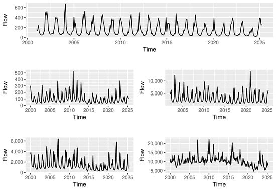
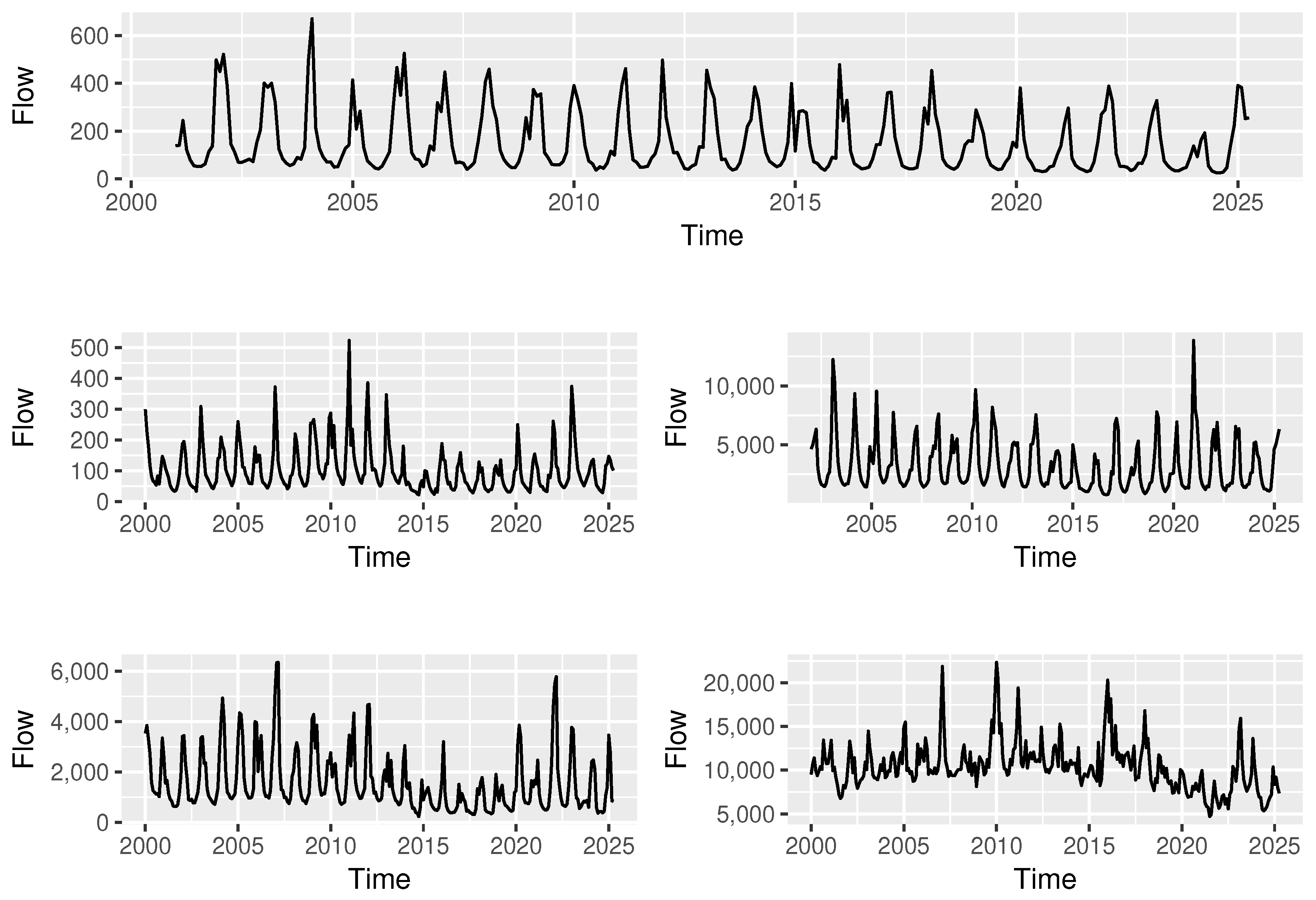
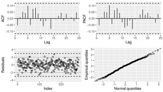
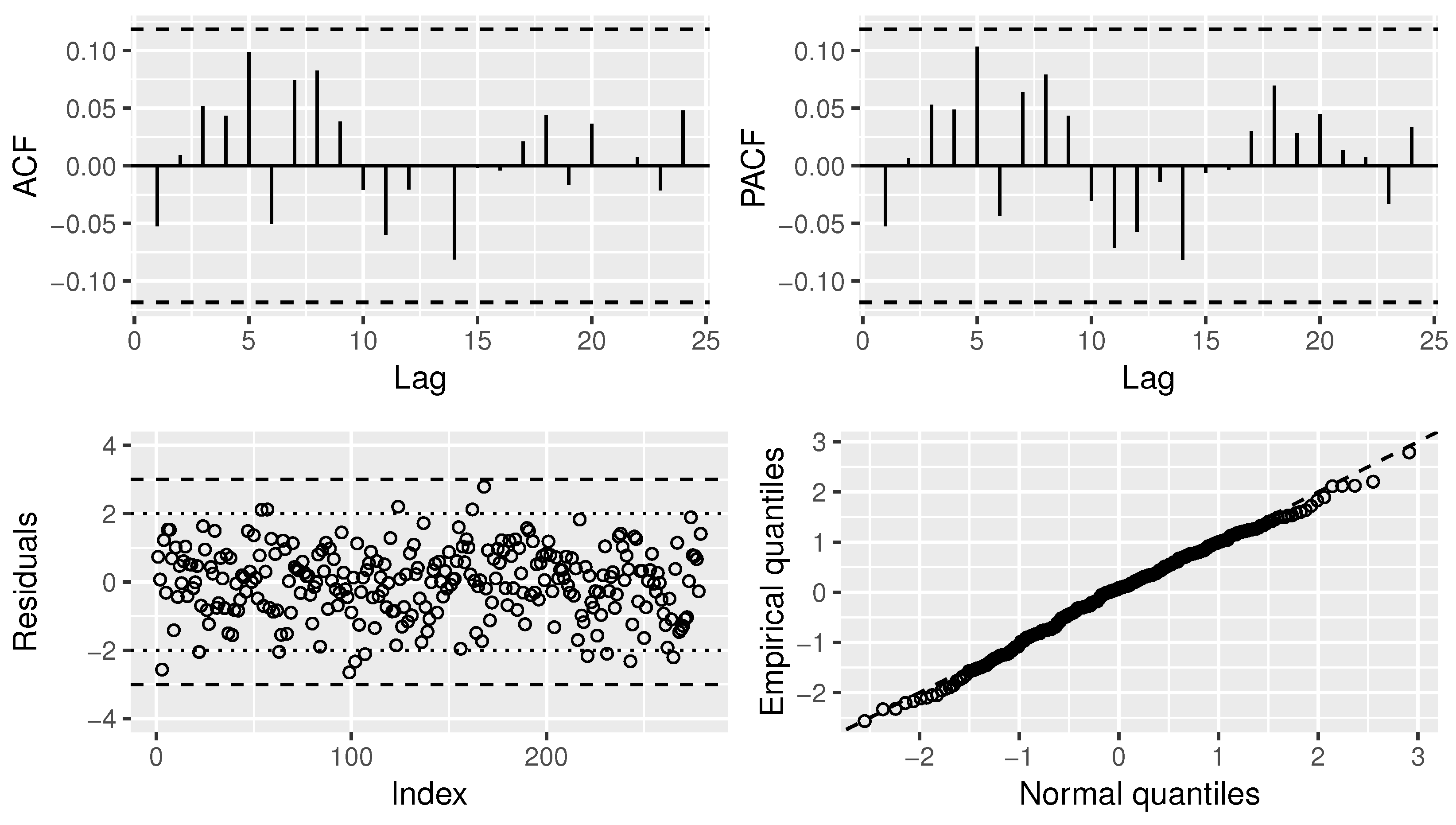
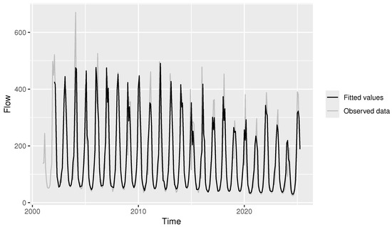
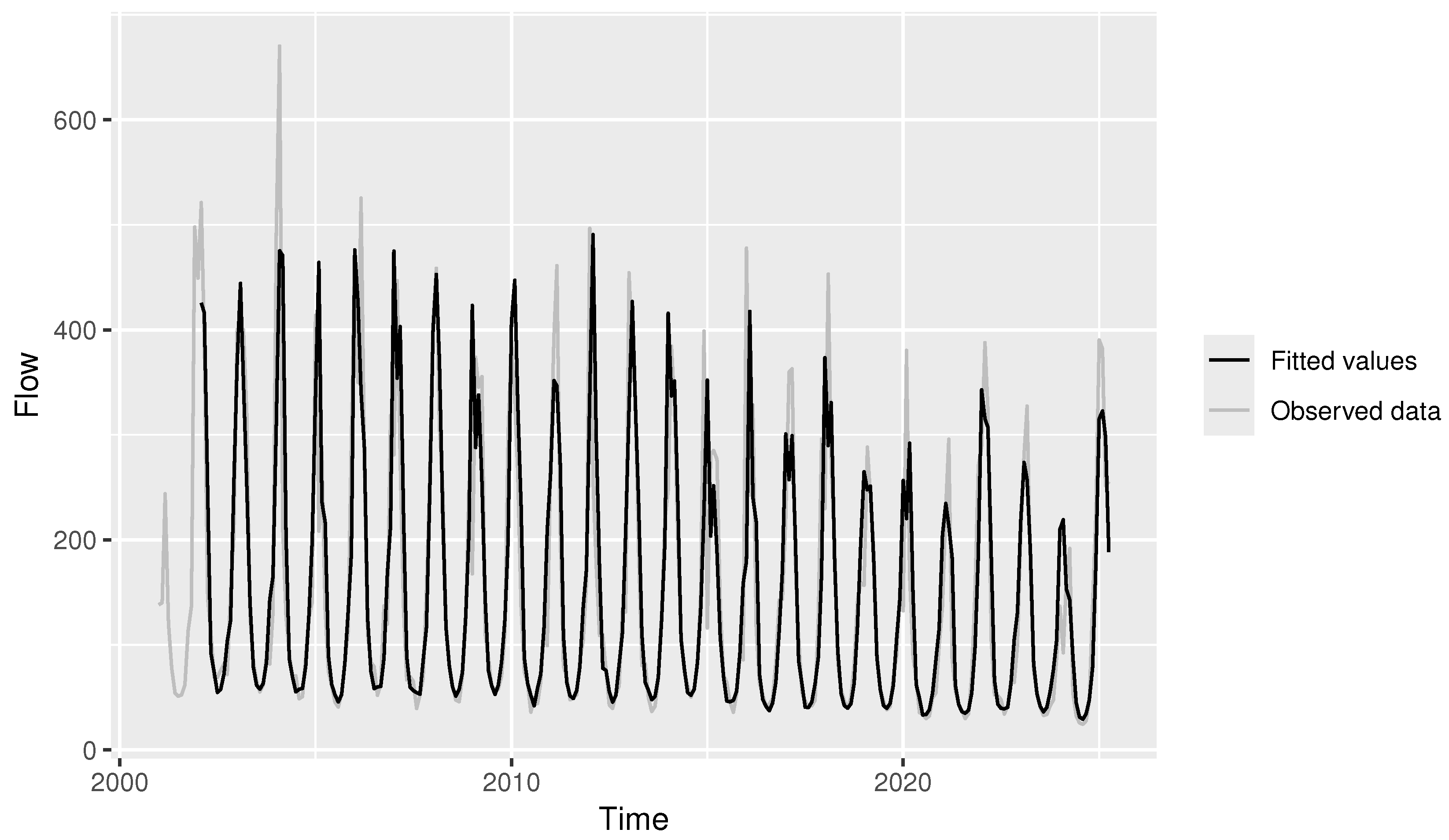
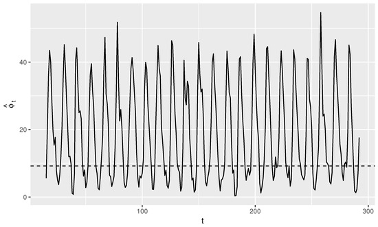
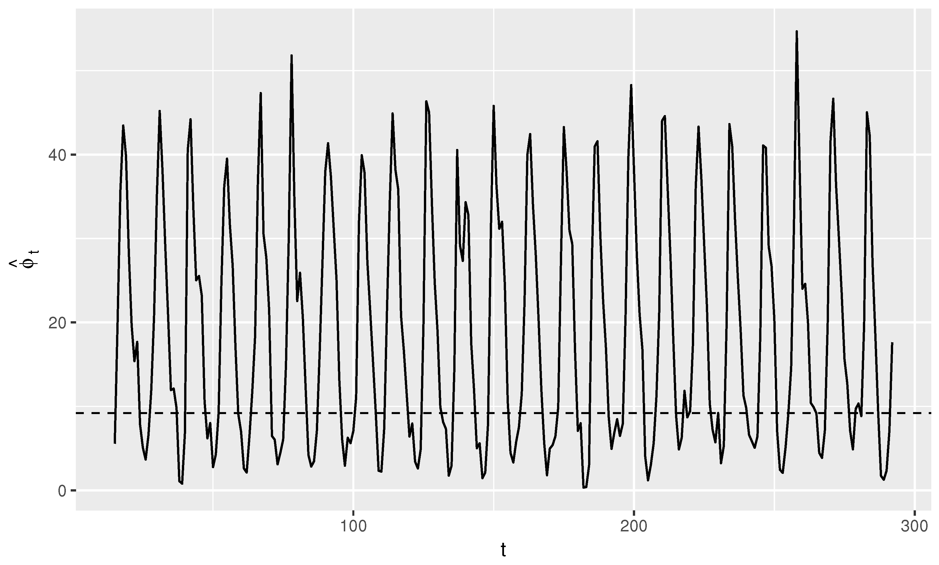

Disclaimer/Publisher’s Note: The statements, opinions and data contained in all publications are solely those of the individual author(s) and contributor(s) and not of MDPI and/or the editor(s). MDPI and/or the editor(s) disclaim responsibility for any injury to people or property resulting from any ideas, methods, instructions or products referred to in the content. |
© 2026 by the authors. Licensee MDPI, Basel, Switzerland. This article is an open access article distributed under the terms and conditions of the Creative Commons Attribution (CC BY) license.