


Abstract
Childhood stunting remains a major public health challenge in India and is influenced by multiple socioeconomic and environmental factors. This ecological study examined district-level correlates of childhood stunting, including Crimes Against Women (CAW), the Multidimensional Poverty Index (MPI), and drought severity, using data from NFHS-5, the National Crime Records Bureau, NITI Aayog’s MPI reports, and the Drought Atlas of India. Spatial autocorrelation and Spatial regression models were applied alongside machine learning approaches and SHAP-based Explainable AI (XAI) interpretation. Childhood stunting exhibited significant spatial clustering (Moran’s I = 0.520, p < 0.001), with hotspots in northern, central, and eastern India. Higher stunting was associated with higher birth order, low maternal BMI, child anaemia, and MPI, and negative associations with iodised salt usage, electricity access, and timely postnatal care. A significant spatial lag parameter (ρ = 0.348) indicated substantial spillover effects. Machine learning models consistently identified MPI, drought severity, and CAW as key predictors. The integrated spatial and machine learning framework identifies key correlates and spatial dependencies of childhood stunting, highlighting the need for region-specific, multisectoral interventions.
1. Introduction
The United Nations adopted the Sustainable Development Goals (SDG Target 2.2) in 2015, aiming to end all forms of malnutrition by 2030 [1]. Globally, during 2022, 148 million (22.3%) children under 5 years were estimated to be stunted (too short for age), 45 million (6.8%) were estimated to be wasted (too thin for height), and 37 million (5.7%) were overweight or living with obesity [2]. Despite sustained global efforts, the 2023 Joint Malnutrition Estimates indicate that progress toward achieving these nutrition targets remains insufficient and requires accelerated action [3].
According to the World Health Organisation (WHO), stunting among children under five in India declined from 41.6% in 2012 to 31.7% in 2022 [4]. To combat malnutrition, the Indian government has implemented programs like the Integrated Child Development Scheme (ICDS) [5], Reproductive and Child Health Program (RCH) [6], National Rural Health Mission (NRHM) [7], Pradhan Mantri Matru Vandana Yojana (PMMVY) [8], Anganwadi Services, targeted schemes for adolescent girls, and POSHAN Abhiyaan [9,10]. However, India still reports the second-highest child stunting in South Asia (38%), after Afghanistan (41%) [11]. With the population projected to increase by 17% from 2022 to 2030, addressing child stunting remains a critical public health priority [12,13,14].
The determinants of stunting are multidimensional, encompassing maternal nutritional status, birth order, household living conditions, access to health services, and exposure to infections [15,16,17,18,19,20,21,22,23]. Emerging evidence further underscores the role of broader structural factors such as climate vulnerability, poverty, and social instability, which often coexist with high levels of child undernutrition [24,25].
Climate-related stressors have been linked to declining food security and heightened nutritional risk across multiple settings [26,27,28,29]. According to UNICEF’s Children’s Climate Risk Index, a substantial proportion of child deaths attributable to climate change are expected to result from undernutrition [30].
The Multidimensional Poverty Index (MPI) captures deprivations in education, health, and living standards that often correspond with spatial patterns of child malnutrition [31,32,33]. Prior studies highlight the strong association between poverty and malnutrition, noting that income-based measures alone are insufficient, and emphasise the need to integrate nutrition indicators within the MPI to better capture the multidimensional nature of deprivation [34,35].
Studies have also documented associations between violence against women and adverse maternal and child outcomes, including compromised nutrition and low birthweight because of domestic violence against women during pregnancy [36,37,38,39].
Given India’s substantial geographic and socio-economic diversity, understanding how these multidimensional district-level characteristics relate to stunting and how they are spatially patterned is essential for designing regionally targeted strategies.
The existing literature indicates that only a limited number of studies have applied spatial analytical methods to examine childhood malnutrition in India, and most have focused primarily on mapping prevalence or identifying regional hotspots [15,16,40]. Few have incorporated spatial lag variables, as the conditions in neighbouring districts may be associated with stunting patterns due to shared socio-economic, environmental, or health-system contexts. The integration of spatial econometric methods with ML remains very limited in malnutrition research, despite their suitability for modelling complex and nonlinear associations. Spatial ML approaches offer enhanced predictive performance when analysing high-dimensional covariates but are often criticised for limited interpretability. Explainable Artificial Intelligence (XAI) techniques, such as SHapley Additive exPlanations (SHAP), provide a principled framework to decompose Machine Learning (ML) predictions and quantify the relative contribution and direction of individual predictors [41,42,43,44]. This study addresses this gap by integrating spatial econometric models, ML algorithms, and XAI to enable robust, interpretable, and spatially informed assessment of childhood stunting determinants.
To the best of our knowledge, no studies in India have simultaneously incorporated spatial lag effects and ML-based predictive interpretation to examine MPI, CAW, drought, and socio-economic determinants as correlates of childhood stunting.
Building on these gaps, the present study (i) investigates the spatial distribution of childhood stunting along with district-level MPI, CAW estimates, and drought severity across India (ii) evaluates the associations between stunting and other multidimensional covariates using spatial econometric models, and (iii) identifies how these variables along with the spatial lag variables, contribute to stunting prediction through spatial machine learning and explainable AI approaches, offering clearer insight into geographically clustered vulnerabilities and supporting more targeted policy responses.
2. Materials and Methods
2.1. Data Sources
This ecological study integrates district-level data from four sources across 692 Indian districts. Data on stunting prevalence (dependent variable) and reliable estimates of key health and nutrition indicators (socioeconomic covariates) were obtained from the National Family Health Survey (NFHS-5), 2019–2021, a comprehensive multi-round survey designed to track health, nutrition, and family welfare metrics [45].
MPI scores (covariate) were sourced from the NITI Aayog Progress Review, based on the Alkire–Foster methodology, and capture deprivations in health, education, and living standards. It utilises 12 indicators, including nutrition, child mortality, maternal health, schooling, and access to basic services like clean water, electricity, and sanitation [46].
District-level relative risks of CAW (covariate) were derived by Pooja et al. [38] using the Besag–York–Mollié model, which accounts for spatial dependence and unstructured heterogeneity. In the study, National Crime Records Bureau (NCRB) data (2020–2022) [47] were analysed using small-area estimation methods and covered multiple CAW categories, including domestic violence, sexual violence against minors, dowry-related offences, rape, abduction, acid attacks, and human trafficking, with overall CAW relative risk computed across the Indian Penal Code and Special and Local Laws.
Drought severity (covariate) was measured using the Standardised Precipitation and Evapotranspiration Index from the Drought Atlas of India, categorising districts into normal, moderate, severe, and extreme drought conditions [48,49,50].
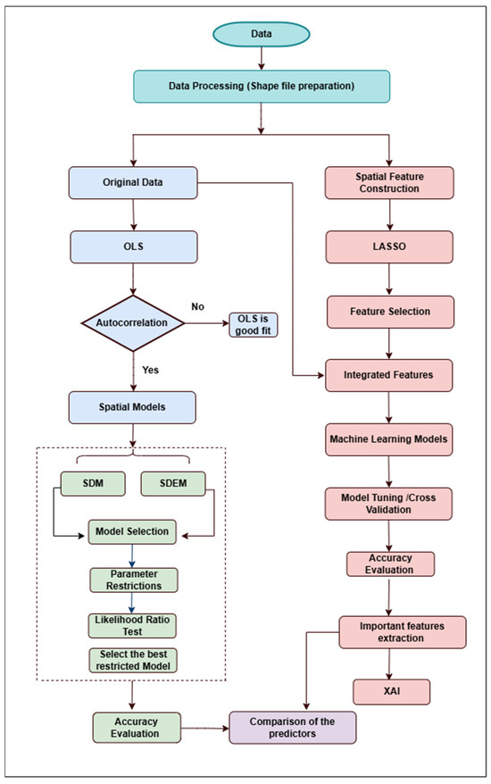
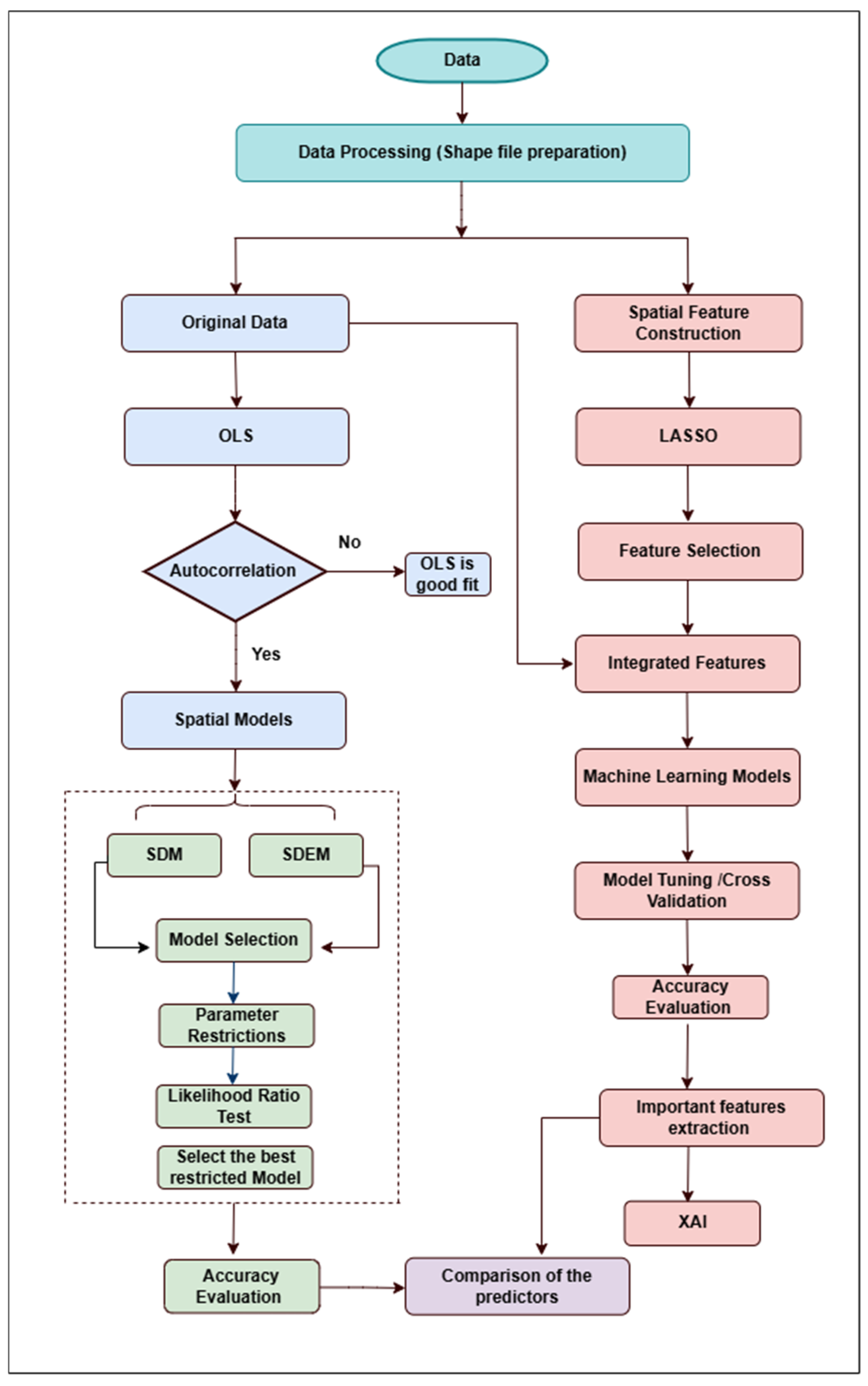
The analytical procedure and modelling approach are depicted in Figure 1.
Figure 1.
Schematic workflow of the study illustrating the analytical framework.
2.2. Spatial Analysis
In the initial phase, the 707-district data were reduced to 692 districts to fit the India shapefile using NFHS-5 district-level data, along with information on CAW, drought, and the MPI [51]. Spatial exploratory data analysis was conducted using Moran’s I and Local Indicators of Spatial Association (LISA) to assess spatial autocorrelation and clustering patterns, implemented via QGIS (v3.38.3) and GeoDa (v1.22) [52,53,54]. An Ordinary Least Squares model was initially applied to identify determinants of childhood stunting, with multicollinearity checked using variance inflation factors (VIF), and residual diagnostics performed using the Jarque-Bera, Breusch-Pagan, and Lagrange Multiplier tests. Upon detecting spatial dependence, spatial econometric models, including the Spatial Durbin model (SDM), Spatial Durbin Error model (SDEM), Spatially Lagged X Model (SLX), Spatial Autoregressive Model (SAR), and Spatial Error Model (SEM), were employed, with model selection guided by the Likelihood Ratio Test (LRT) that simplify the model parameters [55,56,57]. Details provided in the Supplementary File S1.
2.3. Spatial Machine Learning Models and XAI
We then incorporated spatial lag features to capture the influence of neighbouring districts using an ML approach. Random Forest and XGBoost models were then applied using both spatial and spatial lag predictors, following feature selection through the Least Absolute Shrinkage and Selection Operator (LASSO) method [42,43,58,59]. Model interpretability was enhanced using SHAP, which provided transparent insights into how socio-economic characteristics, MPI, drought severity, and CAW indicators contributed to the model’s predictions of childhood stunting [60].
3. Results
3.1. Descriptive Analysis
Descriptive statistics are summarised in Table 1. Descriptive analysis showed that 33.56% of children under five are stunted, with prevalence ranging from a high of 60.6% in Pashchimi Singhbhum (Jharkhand) to a low of 13.2% in Jagatsinghpur (Odisha). Among predictors, the Population living in households with electricity has the highest mean value of 97%, with the minimum at Sitapur (68.35%) in Uttar Pradesh, and nearly 18 districts have the maximum (100%) electric facilities. The average for Households using iodised salt was 95.1%, ranging from Koppal (47.93%) in Karnataka to Khowai (100%) in Tripura. The Population living in households with an improved drinking water source accounted for 93.8%, and 31 of 692 districts had such sources. Nearly 79.2% of Children are receiving postnatal care from a doctor/nurse/LHV/ANM/midwife/other health personnel, whereas the lowest percentage is in Mon (22.6%), Nagaland. The average percentage of Children aged 9–35 months who received a vitamin A dose was 72.5%, with the highest at Mysore (98.1%) in Karnataka and the lowest at Tuensang (27.46%) in Nagaland. Nearly 71.8% of the population lives in households with improved sanitation facilities, with the highest percentage in Malappuram (99.8%) in Kerala and the lowest in Purulia (29.2%) in West Bengal. Children aged 6–59 months who were anaemic accounted for 65.8%, with the highest rate recorded at Leh (95.5%) in Ladakh and the lowest at East Garo Hills (28%) in Meghalaya.
Table 1.
Descriptive statistics and univariate spatial autocorrelation of district-level variables.
3.2. Exploratory Data Analysis
3.2.1. Moran’s Statistic
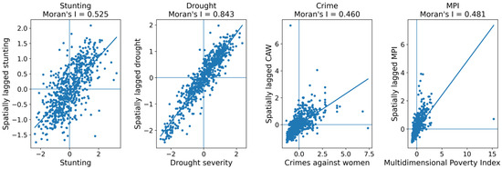
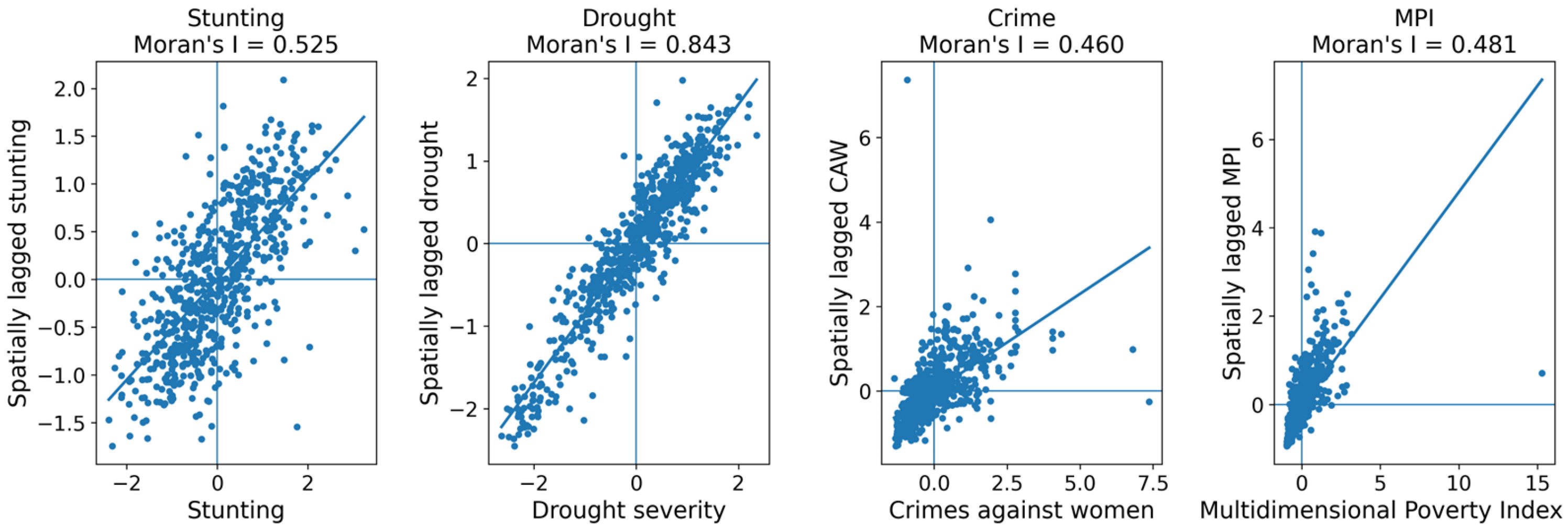
Spatial autocorrelation was assessed using Global Univariate Moran’s I statistic (Table 1). The value for childhood stunting (Moran’s I = 0.525, p < 0.001) indicates a moderate and statistically significant spatial dependency across India. Among the predictors, the highest univariate Moran’s I was observed for drought (0.843), followed by women with BMI below normal (0.729), mothers who consumed iron-folic acid for 180+ days during pregnancy (0.716), and children who received postnatal care (0.709). All these values indicate significant (p < 0.001) strong positive spatial autocorrelation.
Figure 2 presents the Univariate Moran’s Scatterplot: quadrant I groups districts with high values, quadrant III with low values, while quadrants II and IV represent spatial outliers where high and low values are grouped together.
Figure 2.
Univariate Moran’s scatterplots of childhood stunting, drought severity, crime, and MPI.
Bivariate Moran’s I was used to examine spatial correlations between childhood stunting and drought, CAW, and MPI. Moran’s I for stunting and drought was −0.061 (p < 0.05), showing very weak but statistically significant spatial autocorrelation. Stunting and CAW showed a similarly weak negative spatial autocorrelation (Moran’s I = −0.084, p < 0.05). For stunting and MPI, Moran’s I was 0.426 (p < 0.05), reflecting a moderate and significant positive spatial autocorrelation.
3.2.2. Spatial Distribution
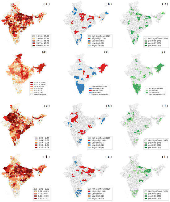
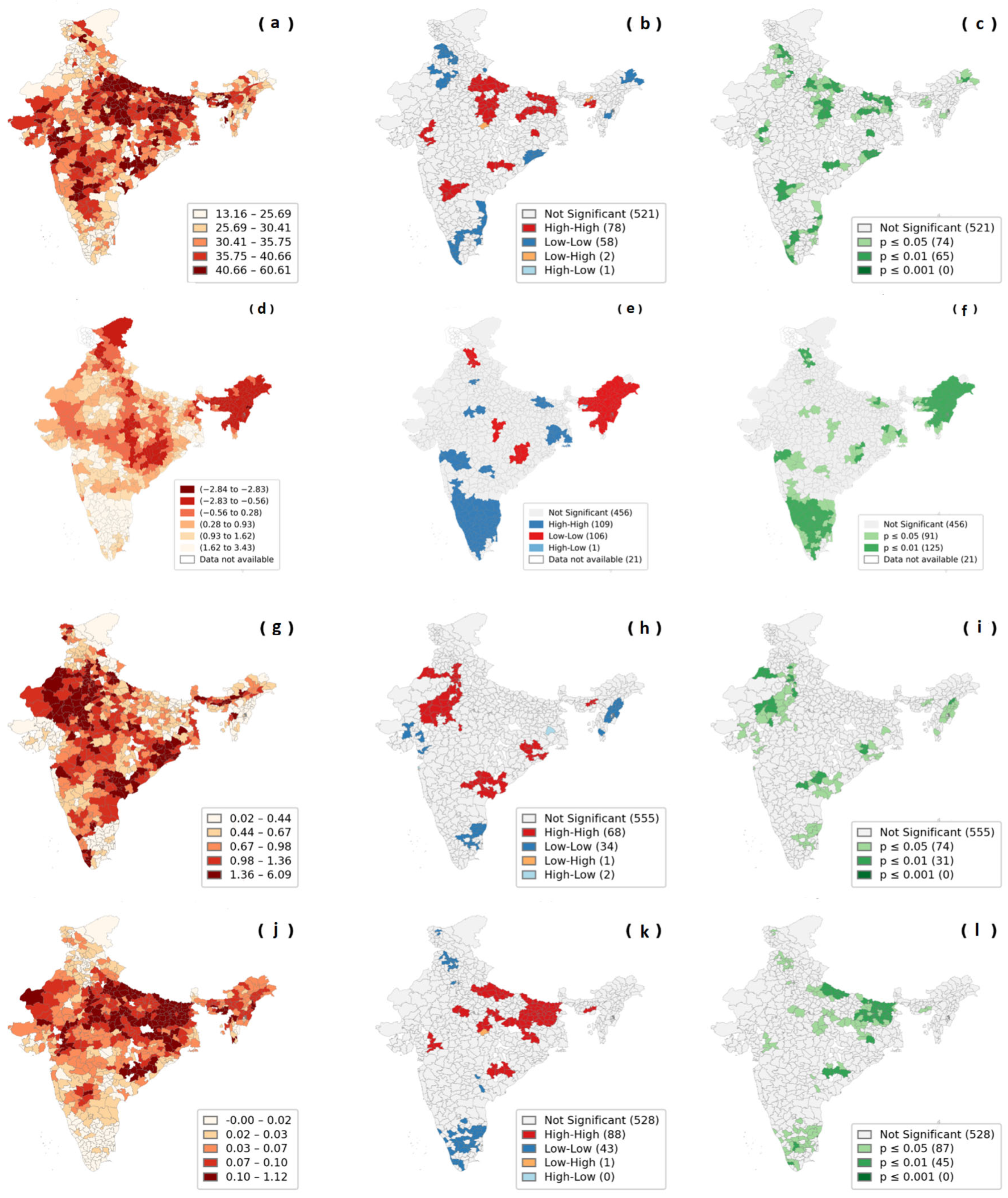
The spatial variation of childhood stunting and its correlates was analysed using spatial maps. Figure 3 presents district-level prevalence, clusters, and their significance.
Figure 3.
Spatial distribution and local spatial autocorrelation of selected factors across 707 districts in India. (a) District level childhood stunting prevalence; (b) LISA cluster map of childhood stunting; (c) LISA significance for childhood stunting; (d) Prevalence of drought severity; (e) LISA cluster map of drought severity; (f) LISA significance for drought severity; (g) Prevalence of crimes against women; (h) LISA cluster map of crimes against women; (i) LISA significance for crimes against women; (j) Prevalence of MPI; (k) LISA cluster map of MPI; (l) LISA significance for MPI.
Stunting: Figure 3a shows the district-level prevalence of childhood stunting across 692 districts, with 78 districts exhibiting the highest stunting rates. Figure 3b,c show that high stunting rates are mainly concentrated in Uttar Pradesh, Bihar, Madhya Pradesh, Gujarat, and Jharkhand, with some parts of Karnataka, Chhattisgarh, Maharashtra, Meghalaya, and Odisha. In contrast, low stunting prevalence is predominantly observed in northern states like Himachal Pradesh and Punjab, and in southern states such as Kerala, Tamil Nadu, and Telangana, reflecting better-performing regions in terms of child stunting
Drought: The district-level prevalence map Figure 3d, shows that 109 of 692 districts experienced the most severe drought conditions. Figure 3e,f illustrate High-High clusters of districts with severe drought surrounded by similarly affected neighbours, primarily concentrated in Northeast India, particularly in Assam and neighbouring states. Additional High-High clusters appear in North India, including parts of Punjab, Haryana, and Uttar Pradesh, and in Central India, particularly in Odisha, Madhya Pradesh, and Chhattisgarh. In contrast, Low-Low clusters of districts with low drought surrounded by similarly less-affected neighbours are mainly located in Southern India, including Tamil Nadu, Karnataka, and Kerala. Some districts in Central India, such as Maharashtra, also exhibit Low-Low clustering.
CAW: The prevalence map for CAW (Figure 3g) identifies 68 districts with the highest CAW rates, predominantly in Northern and Central India. Figure 3h,i highlight hotspots in Uttar Pradesh, Haryana, Rajasthan, and Madhya Pradesh, showing the most significant concentrations of high CAW. Additional elevated CAW levels are observed in parts of Bihar, Gujarat, Chhattisgarh, Maharashtra, and Telangana. Conversely, districts with low CAW rates are concentrated in the Northeast and the South. In the Northeast, Mizoram, Sikkim, and Arunachal Pradesh stand out, while in the South, Kerala, Tamil Nadu, and Andhra Pradesh show the highest concentrations of low-CAW districts. Northern states like Himachal Pradesh and Uttarakhand also exhibit low CAW levels.
MPI: The district-level MPI prevalence map Figure 3j, identifies 88 districts with the highest levels of multidimensional poverty, largely concentrated in North and Western India. These areas are marked by severe deprivations in education, healthcare, and sanitation. Figure 3k,l display High-High clusters prominently found in parts of Uttar Pradesh, Bihar, Meghalaya, Madhya Pradesh, Jharkhand, Odisha, and Chhattisgarh, indicating persistent poverty. In contrast, 43 districts form Low-Low clusters, indicating low MPI surrounded by similarly low-poverty areas.
3.3. Ordinary Least Squares Regression Model
An Ordinary Least Squares regression model was applied to identify key predictors of childhood stunting, using variables with variance inflation factors (VIFs) below 5. Model diagnostics validated the regression assumptions. The Jarque-Bera test confirmed that the residuals were normally distributed (p-value > 0.05), while the Breusch-Pagan test indicated homoskedasticity in the error terms (p-value > 0.05). The Lagrange Multiplier and Robust Lagrange Multiplier tests were both highly significant (p-value < 0.001), indicating spatial dependency in the data.
3.4. Spatial Regression Models
To account for spatial dependency, spatial regression models were applied to identify significant factors associated with childhood stunting. SDM addressed global spatial dependencies, while SDEM focused on local spatial effects. This dual approach allowed a comprehensive analysis of spatial interactions.
Among SDM and SDEM models, the SDM performed better with a lower AIC and higher R2 (AIC = 4344, R2 = 0.6268) compared to the SDEM (AIC = 4348, R2 = 0.6242). Then, to identify the best-fitting spatial model, the SDM was simplified to SLX, SAR, and SEM. LRT showed that the SAR model was the best fit. In the SAR model, 7 of 26 predictors were significantly associated with childhood stunting prevalence. Model details and results are provided in Supplementary File S2. Table 2 presents the estimates for the SDEM, SDM, and SAR models.
Table 2.
Results from spatial econometric models of childhood stunting.
Significant negative associations in the SAR model were observed for electricity (β = −0.19, SE = 0.09, 95% CI: −0.37 to −0.01), iodised salt (β = −0.14, SE = 0.06, 95% CI: −0.26 to −0.02), and postnatal care (β = −0.08, SE = 0.04, 95% CI: −0.16 to −0.002). On average, a 1% increase in these variables may decrease the prevalence of childhood stunting by 0.19%, 0.14%, and 0.08%, respectively. Conversely, significant positive associations were observed for third or higher-order births (β = 0.92, SE = 0.27,95% CI: 0.39 to 1.45), low maternal BMI (β = 0.26, SE = 0.06, 95% CI: 0.14 to 0.38), child anaemia (β = 0.11, SE = 0.04, 95% CI: 0.03 to 0.19), and MPI (β = 12.26, SE = 7.29, 95% CI: −2.03 to 26.55). On average, a 1% increase in these variables may increase stunting prevalence by 0.92%, 0.26%, 0.11%, and 12.26%, respectively.
The significant lag coefficients (ρ = 0.3132 in SDM; ρ = 0.348 in SAR) indicate strong spatial spillover, suggesting that stunting prevalence in a district is statistically associated with stunting levels in neighbouring districts.
3.5. Machine Learning Models
3.5.1. Feature Selection
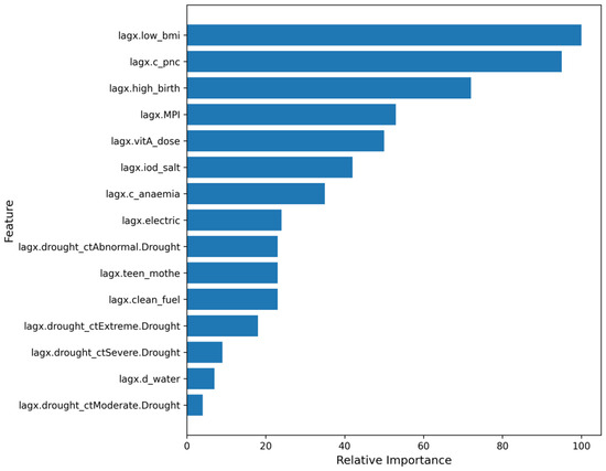
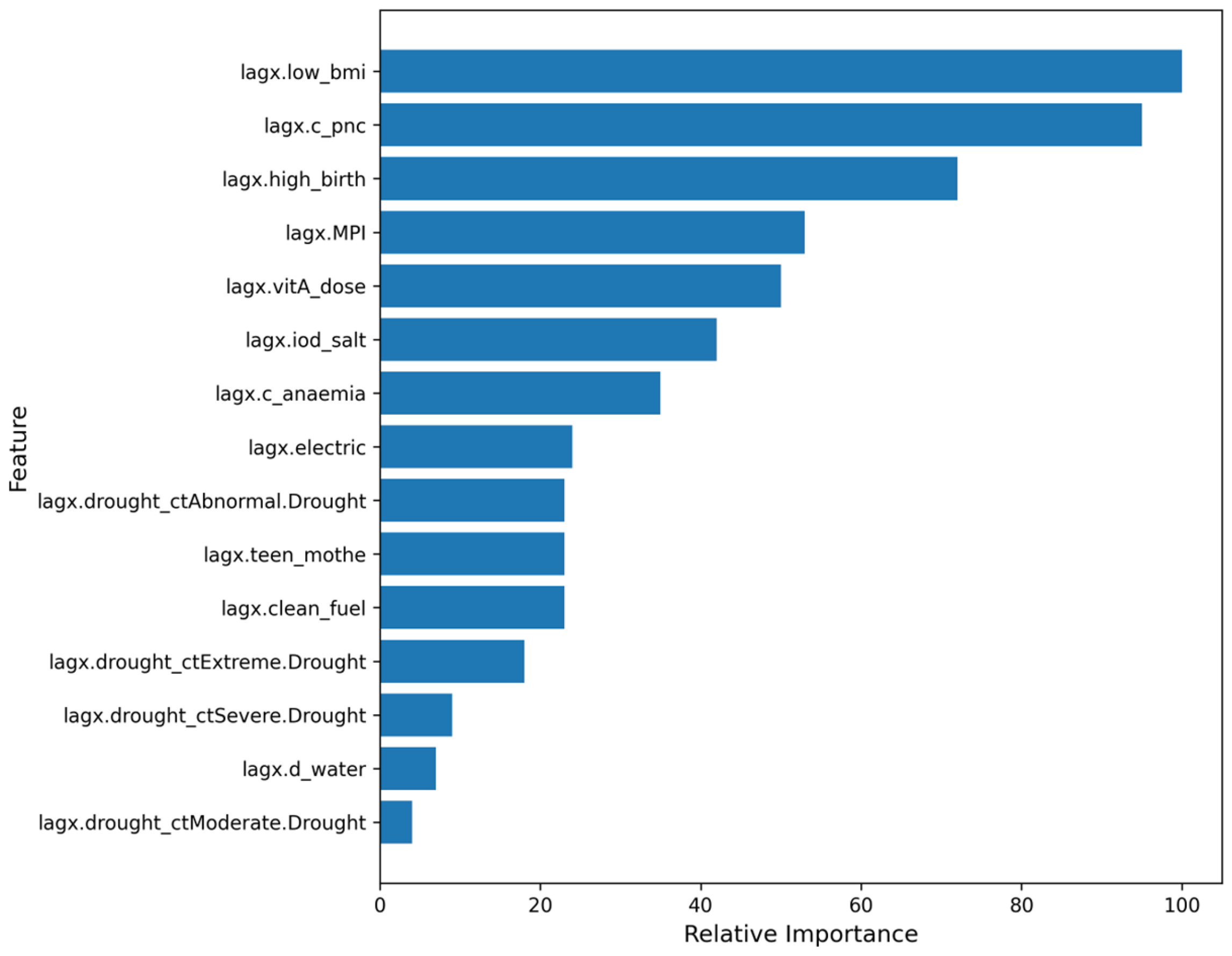
Spatial lag variables were derived from the SLX model to capture neighbourhood dependencies. The most relevant lagged features are selected using LASSO regression, as shown in Figure 4.
Figure 4.
Top 15 spatially lagged variables selected using LASSO regression.
3.5.2. ML Models
After selecting the spatially lagged features, an integrated modelling framework was implemented by combining the original covariates with the selected spatial lag variables in Random Forest and XGBoost models. The dataset was partitioned into training (70%) and independent test (30%) sets, with 10-fold cross-validation applied exclusively to the training data to assess model stability and reduce overfitting.
The Random Forest model was implemented using 500 trees to ensure stable estimation, while other hyperparameters were retained at their default settings to maintain model interpretability in an ecological analysis context in both algorithms. Final model performance was evaluated on the independent test set, and feature importance measures from both models were examined to identify key predictors of childhood stunting.
3.5.3. Variable Importance
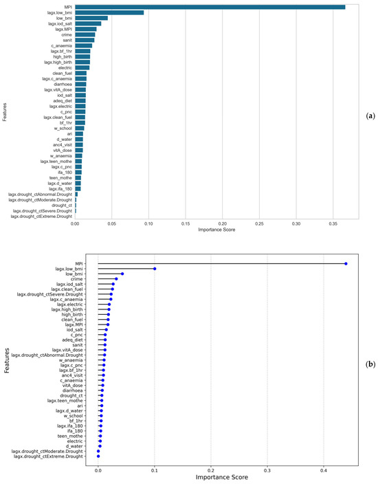
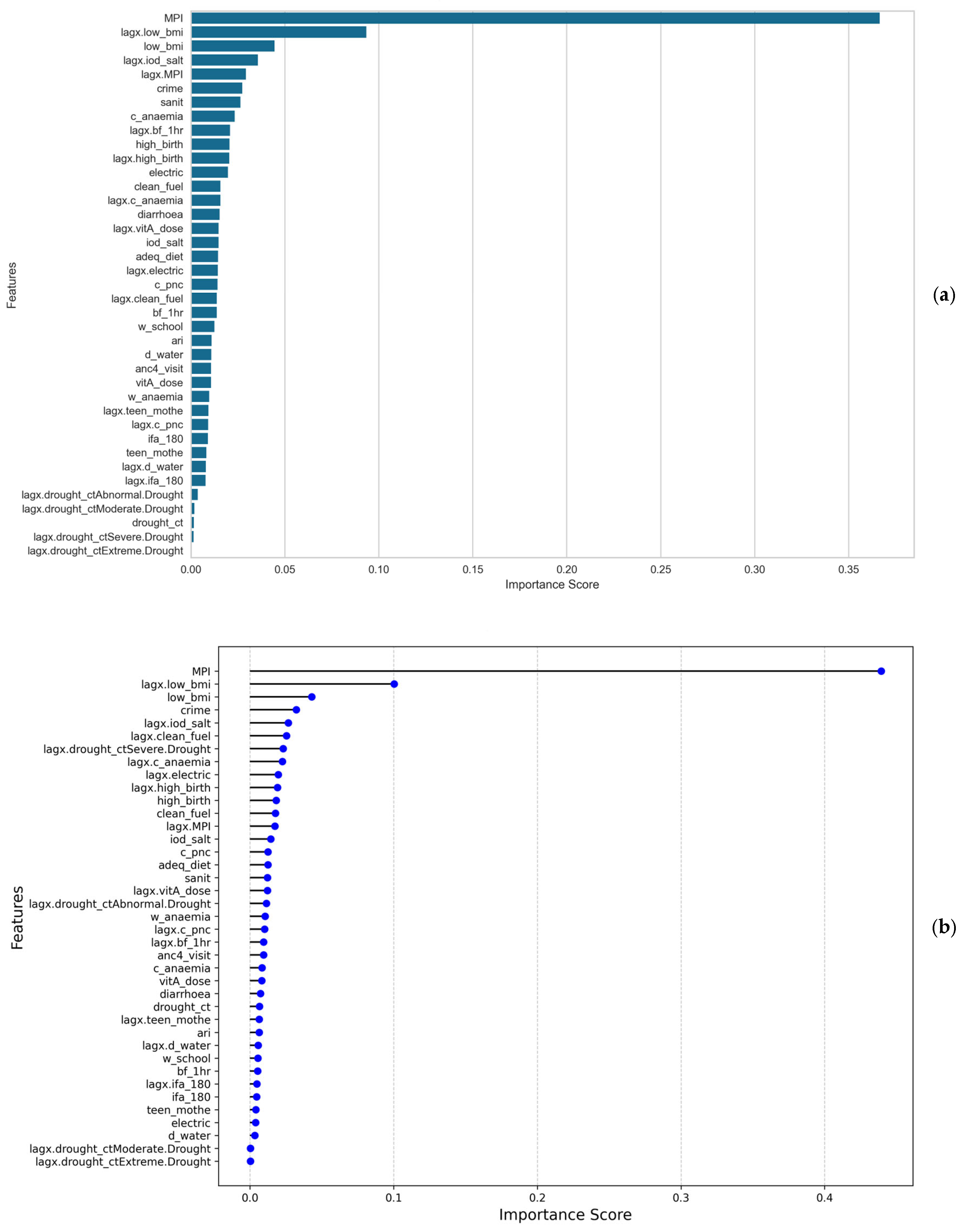
While identifying the important features, both the models consistently highlighted MPI, low BMI, CAW, child anaemia and the infrastructure-related variables, such as access to sanitation, electricity, and clean cooking fuel, as the most significant correlates of stunting prevalence in children. The severe drought variable was an important predictor in the XGBoost model. The important features identified by both algorithms are shown in Figure 5a,b.
Figure 5.
(a) Feature importance from the Random Forest model. (b) Feature importance from the XGBoost model.
3.5.4. Model Evaluation
The Random Forest model could explain approximately 54.8% (R2) of the variance in the target variable. The XGBoost model achieved an R2 score of 0.520, explaining 52.0% of the variance. Akaike Information Criterion (AIC) for the Random Forest model (AIC: 2333.98) was lower compared to the XGBoost model (AIC: 2346.73), indicating a better balance of model complexity and goodness-of-fit for the Random Forest model.
3.6. Explainable Artificial Intelligence
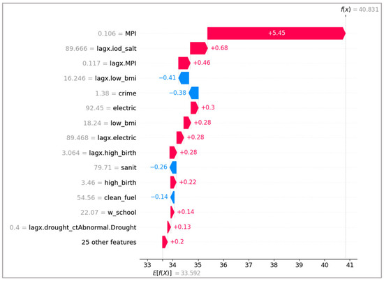
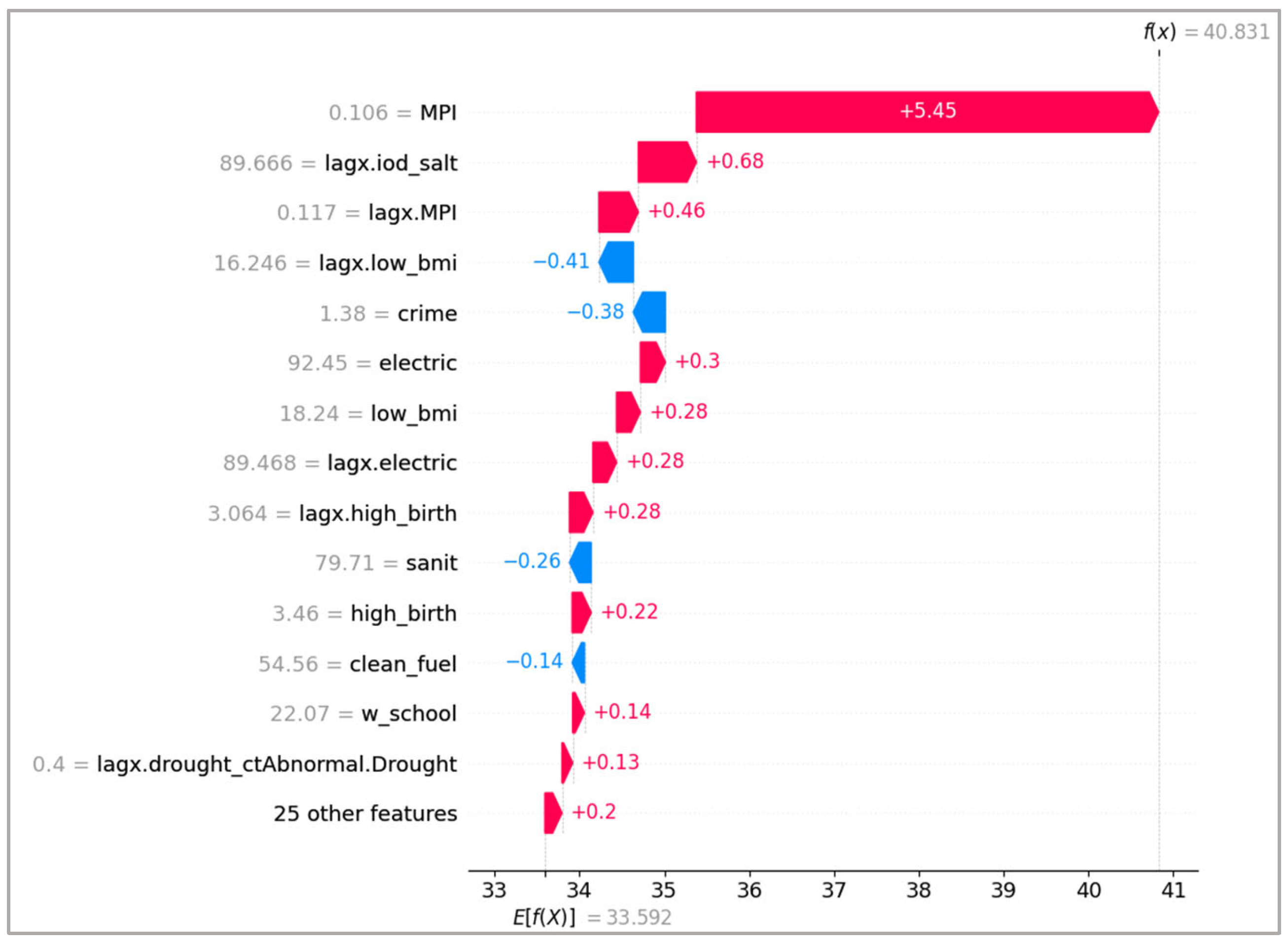
The SHAP analysis decomposed the Random Forest model’s prediction into a baseline and feature-specific contributions. The baseline prediction across districts was 33.592%, while the selected observation had a final predicted stunting level of 40.831%, reflecting a cumulative contribution of +7.239%. Features that increased the predicted value included MPI (+5.45), spatially lagged iodised salt (+0.68), spatially lagged MPI (+0.46), access to electricity (+0.30), women with a below-normal BMI (+0.28), and higher-order birth (+0.28). Smaller contributions from the remaining variables collectively shaped the final model prediction (Figure 6).
Figure 6.
SHAP waterfall plot illustrating feature contributions to model prediction.
4. Discussion
The findings demonstrate pronounced spatial clustering of childhood stunting, with high-prevalence districts concentrated in northern, central, and eastern India [15,17,18,40]. The significant spatial lag coefficients estimated in the SAR and SDM models further indicate substantive spatial spillover effects, implying that stunting levels within a district are statistically associated with those in neighbouring districts. This pattern highlights geographic interdependence and suggests that contextual socio-economic and environmental conditions extend beyond administrative boundaries. These results reinforce the importance of explicitly incorporating spatial structure in nutrition research to ensure valid inference and context-sensitive policy planning [61,62].
Spatial regression models identified several district-level factors significantly associated with childhood stunting. Higher multidimensional poverty, higher birth order, low maternal BMI, and child anaemia were positively associated with increased stunting prevalence [15,16,17,18,19,20,21,22,23,24,25,31,32,33,34,35]. In contrast, improved sanitation, access to electricity, and iodised salt utilisation were associated with lower stunting levels, underscoring the importance of household living conditions and hygiene environments in shaping nutritional outcomes.
Indicators such as drought severity and CAW showed associations in ML models, underscoring the limitations of conventional approaches for capturing complex, nonlinear interactions and for linking environmental and social vulnerability to child nutrition disparities. The role of drought as a significantly associated covariate highlights the need for climate-resilient agricultural and food security policies to mitigate the long-term nutritional consequences of climate variability. Policies aimed at women’s safety, economic empowerment, and access to justice could improve maternal and child health outcomes [26,27,28,29,30,31,32,33,34,35,36,37,38,39,50].
Additionally, the strong association between MPI and stunting, observed in both spatial and ML models, underscores the urgent need for integrated poverty alleviation strategies. Policies should focus on improving access to healthcare, maternal nutrition, education, and sanitation, as these factors directly contribute to reducing childhood malnutrition [62].
The ML models complement spatial regressions by capturing nonlinear relationships and higher-order interactions between spatial and non-spatial variables that are not identifiable within conventional spatial econometric frameworks. Although predictive performance gains between non-spatial and spatial ML models were modest, incorporating spatial lags remains statistically justified, as significant Moran’s I statistics and spatial lag (ρ) coefficients confirm residual spatial dependence in childhood stunting [38,39,40,62]. The presence of spatial autocorrelation violates the independence assumption underlying non-spatial models and indicates potential spatial bias. The spatial model results also demonstrate substantive spillover effects, suggesting that district-level stunting is systematically associated with neighbouring districts, even after controlling locally observed covariates. Thus, incorporating spatial effects strengthens the validity of the estimates and better accounts for geographic dependence, even when improvements in predictive performance are limited [41,42,43]. MPI, drought severity, and CAW emerged as influential contributors to prediction performance, reflecting broader socio-economic and environmental vulnerabilities associated with district-level stunting prevalence [22,27,33,38,39,40,62].
The SHAP analysis enhanced interpretability by decomposing predictions into feature-specific contributions; however, these contributions represent model behaviour rather than causal effects, consistent with recommendations for interpreting explainable AI outputs [41,42,43,44].
Limitations: Despite its strengths, this study has certain limitations. First, the use of district-level aggregated data may bound the importance of within-district heterogeneity in childhood stunting, limiting the ability to identify localised disparities. Second, the spatial weight matrix relies on predefined geographic contiguity, which may not fully reflect social, economic, or environmental interactions across districts. Third, the study doesn’t assess temporal changes or the directionality of observed associations.
5. Conclusions
In summary, the study demonstrated that childhood stunting in India follows distinct spatial patterns shaped by multidimensional socio-economic, social, maternal, environmental, and regional-level characteristics. By integrating spatial econometric models with ML and explainable AI, the analysis reveals important spatial spillover effects and highlights key correlates of district-level stunting patterns. These findings underscore the value of geographically targeted, multisectoral strategies that address shared vulnerabilities across neighbouring districts.
Further exploration using spatial–temporal models or causal inference frameworks may help explain the mechanisms underlying these observed patterns. Additionally, qualitative or mixed-methods research could provide deeper insights into how multidimensional poverty, CAW, and environmental stressors relate to child nutrition at the household and community levels. Strengthening local and regional efforts that consider spatial dependencies may support progress toward reducing undernutrition and advancing national goals aligned with Sustainable Development Goals 2 and 3.
Supplementary Materials
The following supporting information can be downloaded at: https://www.mdpi.com/article/10.3390/stats9020034/s1.
Author Contributions
Design and concept: B.R. and M.G.H.; Data acquisition: B.R.; Data analysis: B.R. and M.G.H.; Data Interpretation: B.R. and M.G.H.; Drafting of the first version of the manuscript: B.R. Conceptualization, B.R. and M.G.H.; methodology, B.R. and M.G.H.; software, B.R.; validation, B.R.; formal analysis, B.R. and B.P.; resources, B.R. and A.K.; writing—original draft preparation, B.R.; writing—review and editing, B.R., M.G.H., A.K., M.A. and Y.M.E.; visualization, B.R.; supervision, M.G.H., A.K., M.A. and Y.M.E. All authors have read and agreed to the published version of the manuscript.
Funding
This work was supported by the Deanship of Scientific Research Vice Presidency for Graduate studies and Scientific Research, King Faisal University, Saudi Arabia [Grant No. KFU261092].
Informed Consent Statement
This study utilises publicly available datasets, including the National Family Health Survey-5, National Crime Records Bureau data, and Drought Index data. Since these datasets are open source and publicly accessible, no separate ethical approval or consent for publication was required.
Data Availability Statement
The original contributions presented in this study are included in the article/Supplementary Materials. Raw data sets are publicly available and can be accessed via the provided weblinks. NFHS 5 District-level Data: https://www.data.gov.in/resource/india-districts-factsheets-national-family-health-survey-nfhs-5-2019-2021-provisional (accessed on 16 July 2025). Drought status: https://zenodo.org/records/8280551 (accessed on 16 July 2025). Multidimensional Poverty Index: https://niti.gov.in/publications/division-reports (accessed on 16 July 2025). District-level relative risks of crime against women: https://doi.org/10.3389/fpubh.2024.1362406. Further inquiries can be directed at the corresponding author(s).
Acknowledgments
The authors are grateful to the reviewers and the journal editor for their valuable comments and suggestions, which have significantly improved the manuscript.
Conflicts of Interest
The author(s) declared no potential conflicts of interest with respect to the research, authorship, and/or publication of this article.
Abbreviations
The following abbreviations are used in this manuscript:
| CAW | Crimes Against Women |
| MPI | Multidimensional Poverty Index |
| ML | Machine Learning |
| XAI | Explainable AI |
| SHAP | SHapley Additive exPlanations |
| NFHS | National Family Health Survey |
| NCRB | National Crime Records Bureau |
| LISA | Local Indicators of Spatial Association |
| SDM | Spatial Durbin Model |
| SDEM | Spatial Durbin Error model |
| SLX | Spatially Lagged X Model |
| SAR | Spatial Autoregressive Model |
| SEM | Spatial Error Model |
| LRT | Likelihood Ratio Test |
| LASSO | Least Absolute Shrinkage and Selection Operator |
References
- United Nations System Standing Committee on Nutrition. Nutrition and the Post-2015 Sustainable Development Goals. Available online: https://www.unnutrition.org/library/briefs/nutrition-and-post-2015-sustainable-development-goals (accessed on 16 July 2025).
- World Health Organisation. Malnutrition Key Facts. 2024. Available online: https://www.who.int/news-room/fact-sheets/detail/malnutrition (accessed on 15 July 2025).
- UNICEF. UNICEF-WHO-The World Bank: Joint Child Malnutrition Estimates (JME). In Levels and Trends in Child Malnutrition, 2023rd ed.; UNICEF: New York, NY, USA, 2023; Available online: https://data.unicef.org/wp-content/uploads/2023/05/JME-2023-Levels-and-trends-in-child-malnutrition.pdf (accessed on 16 July 2025).
- DTE Staff. India’s Child Wasting Rate 18.7% as per Latest UN Inter-Agency Estimates. Available online: https://www.downtoearth.org.in/health/india-s-child-wasting-rate-18-7-as-per-latest-un-inter-agency-estimates-89586 (accessed on 16 July 2025).
- Singh, S.K.; Chauhan, A.; Alderman, H.; Avula, R.; Dwivedi, L.K.; Kapoor, R.; Meher, T.; Menon, P.; Nguyen, P.H.; Pedgaonker, S.; et al. Utilization of Integrated Child Development Services (ICDS) and its linkages with undernutrition in India. Matern. Child Nutr. 2024, 20, e13644. [Google Scholar] [CrossRef] [Scilit] [PubMed]
- Ministry of Health and Family Welfare, Government of India. Reproductive and Child Health (RCH) Portal. Available online: https://rch.mohfw.gov.in/RCH/about-rch.aspx (accessed on 16 July 2025).
- Nandan, D. National rural health mission: Turning into reality. Indian J. Community Med. 2010, 35, 453–454. [Google Scholar] [CrossRef] [Scilit] [PubMed]
- Behera, S. Pradhan Mantri Matru Vandana Yojana (PMMVY): A Review. Int. J. Home Sci. 2023, 9, 11–15. [Google Scholar] [CrossRef]
- Paul, V.K.; Singh, A.; Palit, S. POSHAN Abhiyaan: Making nutrition a Jan Andolan. Proc. Indian Natl. Sci. Acad. 2018, 84, 835–841. [Google Scholar]
- Kapur, K.; Suri, S. Towards a Malnutrition-Free India: Best Practices and Innovations from POSHAN Abhiyaan. Observer Research Foundation. 2020. Available online: https://www.orfonline.org/research/towards-a-malnutrition-free-india-63290 (accessed on 20 July 2025).
- World Bank Group. Tackling Malnutrition in South Asia: 8 Years on. End Poverty in South Asia. 2024. Available online: https://blogs.worldbank.org/en/endpovertyinsouthasia/tackling-malnutrition-south-asia-8-years (accessed on 21 July 2025).
- World Health Organization. WHO Data: India (Country Code 356). 2024. Available online: https://data.who.int/countries/356 (accessed on 30 June 2025).
- United Nations Children’s Fund (UNICEF). UNICEF Conceptual Framework on Maternal and Child Nutrition; UNICEF: New York, NY, USA, 2021; Available online: https://www.unicef.org/nutrition (accessed on 1 July 2025).
- Dijkzeul, D. United Nations Children’s Fund Annual Report 2023. UNICEF. 2023. Available online: https://www.unicef.org/reports/unicef-annual-report-2023 (accessed on 2 August 2025).
- Puri, P.; Khan, J.; Shil, A.; Ali, M. A cross-sectional study on selected child health outcomes in India: Quantifying the spatial variations and identification of the parental risk factors. Sci. Rep. 2020, 10, 6645. [Google Scholar] [CrossRef] [Scilit] [PubMed]
- Nambiar, A.; Agnihotri, S.B.; Arunachalam, D.; Singh, A. Undernutrition among children and its determinants across the parliamentary constituencies of India: A geospatial analysis. J. Biosoc. Sci. 2024, 56, 338–356. [Google Scholar] [CrossRef] [Scilit]
- Khare, S.; Kavyashree, S.; Gupta, D.; Jyotishi, A. Investigation of nutritional status of children based on machine learning techniques using Indian demographic and health survey data. Procedia Comput. Sci. 2017, 115, 338–349. [Google Scholar] [CrossRef] [Scilit]
- Vasu, S.R.; Khare, S.; Gupta, D.; Jyotishi, A. Features Explaining Malnutrition in India: A Machine Learning Approach to Demographic and Health Survey Data. In Proceedings of the International Advanced Computing Conference; Springer: Singapore, 2020; pp. 87–99. [Google Scholar]
- Jain, S.; Khanam, T.; Abedi, A.J.; Khan, A.A. Efficient Machine Learning for Malnutrition Prediction among under-five children in India. In Proceedings of the 2022 IEEE Delhi Section Conference (DELCON); IEEE: New York, NY, USA, 2022; pp. 1–10. [Google Scholar]
- Saroj, R.K.; Yadav, P.K.; Singh, R.; Chilyabanyama, O.N. Machine Learning Algorithms for understanding the determinants of under-five Mortality. BioData Min. 2022, 15, 20. [Google Scholar] [CrossRef] [Scilit]
- Seth, P.; Jain, P. What are the key determinants of child malnutrition in India? Empirical evidence from NFHS-4. Indian Econ. J. 2023, 71, 729–747. [Google Scholar] [CrossRef] [Scilit]
- Joseph, R.; Sawant, V.; Shenai, S.; Paryani, M.; Patil, G. Machine learning based factors affecting malnutrition and anemia among children in india. In Proceedings of the 2022 6th International Conference on Intelligent Computing and Control Systems (ICICCS); IEEE: New York, NY, USA, 2022; pp. 1826–1833. [Google Scholar]
- Kishore, K.K.; Suman, J.V.; Mnikyamba, I.L.; Polamuri, S.R.; Venkatesh, B. Prediction of Malnutrition in Newborninfants Using Machine Learning Techniques; Research Square: Durham, NC, USA, 2023. [Google Scholar]
- Population Council. Children in Indian Districts with High Climate Vulnerability More Likely to Suffer from Malnutrition. New Delhi: Population Council. 2022. Available online: https://popcouncil.org/insight/children-in-indian-districts-with-high-climate-vulnerability-more-likely-to-suffer-from-malnutrition (accessed on 3 August 2025).
- Sabri, B.; Khan, N.A.; Tahir, M.; Khan, M.A.; Khan, M.N. Impact of domestic violence on maternal and child health and well-being in rural India. J. Fam. Violence 2025, 40, 435–450. [Google Scholar] [CrossRef] [Scilit]
- World Food Programme. Climate Crisis and Malnutrition: A Case for Acting Now. Saving Lives, Changing Lives. WFP. 2021. Available online: https://www.wfp.org/publications/climate-crisis-and-malnutrition-case-acting-now (accessed on 30 September 2025).
- Mahapatra, B.; Walia, M.; Rao, C.A.; Raju, B.M.; Saggurti, N. Vulnerability of agriculture to climate change increases the risk of child malnutrition: Evidence from a large-scale observational study in India. PLoS ONE 2021, 16, e0253637. [Google Scholar] [CrossRef] [Scilit]
- Thiede, B.C.; Gray, C. Climate exposures and child undernutrition: Evidence from Indonesia. Soc. Sci. Med. 2020, 265, 113298. [Google Scholar] [CrossRef] [Scilit] [PubMed]
- Thiede, B.C.; Strube, J. Climate variability and child nutrition: Findings from sub-Saharan Africa. Glob. Environ. Change 2020, 65, 102192. [Google Scholar] [CrossRef] [Scilit] [PubMed]
- He, B.J.; Prasad, D.; Pignatta, G.; Jupesta, J. (Eds.) Climate Change and Environmental Sustainability; Springer: Berlin/Heidelberg, Germany, 2022. [Google Scholar]
- D’Attoma, I.; Matteucci, M. Multidimensional poverty: An analysis of definitions, measurement tools, applications and their evolution over time through a systematic review of the literature up to 2019. Qual. Quant. 2024, 58, 3171–3213. [Google Scholar] [CrossRef] [Scilit]
- Das, P.; Ghosh, S.; Paria, B. Multidimensional poverty in India: Patterns of reduction across population subgroups and geographical locations during 2005–2006 and 2019–2021. GeoJournal 2023, 88, 3851–3870. [Google Scholar] [CrossRef] [Scilit]
- Kandapan, B.; Pradhan, J.; Pradhan, I. An individual-specific approach to multidimensional child poverty in India: A study of regional disparities. Child Indic. Res. 2023, 16, 2075–2105. [Google Scholar] [CrossRef] [Scilit]
- Siddiqui, F.; Salam, R.A.; Lassi, Z.S.; Das, J.K. The intertwined relationship between malnutrition and poverty. Front. Public Health 2020, 8, 453. [Google Scholar] [CrossRef] [Scilit] [PubMed]
- Dele, M. Multidimensional Poverty and Its Determinants: Empirical Evidence from Nigeria. Munich Personal RePEc Archive. 2020. Available online: https://mpra.ub.uni-muenchen.de/101842 (accessed on 29 July 2025).
- Pakrashi, D.; Saha, S. Intergenerational consequences of spousal violence: Effect on nutritional status of children. Rev. Econ. Househ. 2024, 22, 67–94. [Google Scholar] [CrossRef] [Scilit]
- Ackerson, L.K.; Subramanian, S. Domestic violence and chronic malnutrition among women and children in India. Am. J. Epidemiol. 2008, 167, 1188–1196. [Google Scholar] [CrossRef] [Scilit]
- Pooja, B.S.; Guddattu, V.; Rao, K.A. Crime against women in India: District-level risk estimation using the small area estimation approach. Front. Public Health 2024, 12, 1362406. [Google Scholar] [CrossRef] [Scilit]
- Guo, C.; Wan, M.; Wang, Y.; Wang, P.; Tousey-Pfarrer, M.; Liu, H.; Yu, L.; Jian, L.; Zhang, M.; Yang, Z.; et al. Associations between intimate partner violence and adverse birth outcomes during pregnancy: A systematic review and meta-analysis. Front. Med. 2023, 10, 1140787. [Google Scholar] [CrossRef] [Scilit]
- Mishra, R.; Bera, S. Geospatial and environmental determinants of stunting, wasting, and underweight: Empirical evidence from rural South and Southeast Asia. Nutrition 2024, 120, 112346. [Google Scholar]
- Zhang, X.; Usman, M.; Irshad, A.U.; Rashid, M.; Khattak, A. Investigating spatial effects through machine learning and leveraging explainable AI for child malnutrition in Pakistan. ISPRS Int. J. Geo-Inf. 2024, 13, 330. [Google Scholar] [CrossRef] [Scilit]
- Liu, X.; Kounadi, O.; Zurita-Milla, R. Incorporating spatial autocorrelation in machine learning models using spatial lag and eigenvector spatial filtering features. ISPRS Int. J. Geo-Inf. 2022, 11, 242. [Google Scholar] [CrossRef] [Scilit]
- Usman, M.; Kopczewska, K. Spatial and machine learning approach to model childhood stunting in Pakistan: Role of socio-economic and environmental factors. Int. J. Environ. Res. Public Health 2022, 19, 10967. [Google Scholar] [CrossRef] [Scilit] [PubMed]
- Rao, B.; Rashid, M.; Hasan, M.G.; Thunga, G. Machine Learning in Predicting Child Malnutrition: A Meta-Analysis of Demographic and Health Surveys Data. Int. J. Environ. Res. Public Health 2025, 22, 449. [Google Scholar] [CrossRef] [Scilit] [PubMed]
- 45. International Institute for Population Sciences (IIPS) and ICF. National family health survey(NFHS-5) India 2019–2021. Demogr. Heal. Surv. 2021, 1–714. Available online: https://dhsprogram.com/methodology/survey/survey-display-541.cfm (accessed on 4 June 2025).
- NITI Aayog, Government of India. National Multidimensional Poverty Index: A Progress Review 2023. Available online: https://niti.gov.in/publications/division-reports (accessed on 10 June 2025).
- National Crime Records Bureau. Crime in India 2020: All Publications Year-Wise. Available online: https://www.ncrb.gov.in/crime-in-india-year-wise.html?year=2020&utm_source=chatgpt.com (accessed on 20 June 2025).
- Chuphal, V.; Kushwaha, D.S.; Aadhar, S.; Mishra, V. Drought Atlas of India, 1901–2020. 2023. Available online: https://zenodo.org/records/8280551 (accessed on 5 June 2025).
- Aadhar, S.; Mishra, V. High-resolution near real-time drought monitoring in South Asia. Sci. Data 2017, 4, 170145. [Google Scholar] [CrossRef] [Scilit]
- Carbone, G.J.; Rhee, J.; Mizzell, H.P.; Boyles, R. A regional-scale drought monitoring tool for the Carolinas. Bull. Am. Meteorol. Soc. 2008, 89, 20–28. [Google Scholar] [CrossRef]
- Kumar, D.K.P. India 2020 District Level Shape Files. Kaggle. 2020. Available online: https://www.kaggle.com/datasets/imdevskp/india-district-wise-shape-files (accessed on 2 January 2025).
- Fischer, M.M.; Wang, J. Spatial Data Analysis: Models, Methods and Techniques. In Science & Business Media; Springer: Berlin/Heidelberg, Germany, 2011. [Google Scholar]
- Anselin, L. Local indicators of spatial association—LISA. Geogr. Anal. 1995, 27, 93–115. [Google Scholar] [CrossRef] [Scilit]
- Choi, M. Book Review: Spatial Analysis in Epidemiology. Healthc. Inform. Res. 2013, 19, 148–149. [Google Scholar] [CrossRef] [Scilit]
- Larch, M.; Walde, J. Lag or error?—Detecting the nature of spatial correlation. In Data Analysis, Machine Learning and Applications: Proceedings of the 31st Annual Conference of the Gesellschaft für Klassifikation e.V., Albert-Ludwigs-Universität Freiburg, 7–9 March 2007; Springer: Berlin/Heidelberg, Germany, 2008; pp. 301–308. [Google Scholar]
- Golgher, A.B.; Voss, P.R. How to interpret the coefficients of spatial models: Spillovers, direct and indirect effects. Spat. Demogr. 2016, 4, 175–205. [Google Scholar] [CrossRef] [Scilit]
- Agiakloglou, C.; Tsimpanos, A. Evaluating the performance of AIC and BIC for selecting spatial econometric models. J. Spat. Econom. 2023, 4, 2. [Google Scholar] [CrossRef] [Scilit]
- Tibshirani, R. Regression shrinkage and selection via the lasso. J. R. Stat. Soc. Ser. B Stat. Methodol. 1996, 58, 267–288. [Google Scholar] [CrossRef] [Scilit]
- Friedman, J.H.; Hastie, T.; Tibshirani, R. Regularization paths for generalized linear models via coordinate descent. J. Stat. Softw. 2010, 33, 1–22. [Google Scholar] [CrossRef] [Scilit] [PubMed]
- Dikshit, A.; Pradhan, B. Interpretable and explainable AI (XAI) model for spatial drought prediction. Sci. Total Environ. 2021, 801, 149797. [Google Scholar] [CrossRef] [Scilit] [PubMed]
- Striessnig, E.; Bora, J.K. Under-five child growth and nutrition status: Spatial clustering of Indian districts. Spat. Demogr. 2020, 8, 63–84. [Google Scholar] [CrossRef] [Scilit]
- Biswas, M. Identifying geographical heterogeneity in associations between under-five child nutritional status and its correlates across Indian districts. Spat. Demogr. 2022, 10, 143–187. [Google Scholar] [CrossRef] [Scilit]

Disclaimer/Publisher’s Note: The statements, opinions and data contained in all publications are solely those of the individual author(s) and contributor(s) and not of MDPI and/or the editor(s). MDPI and/or the editor(s) disclaim responsibility for any injury to people or property resulting from any ideas, methods, instructions or products referred to in the content. |
© 2026 by the authors. Licensee MDPI, Basel, Switzerland. This article is an open access article distributed under the terms and conditions of the Creative Commons Attribution (CC BY) license.