An Adaptive Method to Identify Outliers in Skewed Observations: Application to Assess NAACCR Cancer Registry Data Usage

Abstract

Outlier detection is a fundamental component of data preprocessing and quality monitoring across diverse scientific domains, including engineering, biomedical sciences, and finance. While many variables in controlled environments approximate a normal distribution, real-world data, particularly biological, environmental, and epidemiological measures, are frequently characterized by pronounced right-skewness. To address the shortcomings of conventional methods, this study introduces the Dynamic Threshold for Outlier Detection (DTOD), which reframes outlier detection as a concrete operational workflow. The DTOD framework dynamically adjusts detection thresholds based on a functional relationship between skewness and tail morphology. Validation through large-scale simulation experiments across light-, middle-, and high-skewness levels confirms the method’s versatility. The DTOD proves particularly effective at two ends of the spectrum: enhancing sensitivity for detecting subtle anomalies in light-skewed data while serving as a conservative, high-confidence screening tool that controls false positives in high-skewness environments. In real-world application to North American Association of Central Cancer Registries (NAACCR) data, the method successfully identified outliers with abnormally high unknown tumor size rates in colorectal cancer and maintained a low misclassification rate in highly skewed lung cancer data. Ultimately, the DTOD provides a promising, interpretable solution for improving data quality in skewed scenarios.

1. Introduction

Outlier detection is a fundamental component of data preprocessing and quality monitoring across diverse scientific domains, including engineering, biomedical sciences, and finance. Accurately identifying outliers is an essential step in data cleaning and analysis and is a prerequisite for drawing valid conclusions, as these anomalies can distort descriptive statistics, reduce parameter estimation accuracy, and impair predictive performance. While many variables in controlled environments approximate a normal distribution, real-world data, particularly biological, environmental, and epidemiological measures, are frequently characterized by pronounced right-skewness [1,2,3].

A variety of outlier detection methods have been developed, but each has limitations when applied to skewed data. Conventional distribution-based methods, such as the Z-score [4] or Grubbs’ test [5], assume symmetry and perform poorly in the presence of skewness. Under such conditions, fixed-threshold methods tend to suffer from high false-positive rates in heavily skewed contexts or insufficient sensitivity in lightly skewed scenarios [6,7]. Even robust statistical approaches like the modified Z-score, which replaces mean and standard deviation with median and median absolute deviation (MAD), respectively, while resistant to extreme values, often rely on symmetric cut-offs that may overlook subtle anomalies [7,8]. Leys et al. [8] argued for the superiority of median-based alternatives over mean-based statistics in outlier detection, yet symmetric application remains a limitation. Beyond symmetric robust methods, the statistical literature has established frameworks for skewness-aware outlier detection. Notably, Hubert and Vandervieren [9] introduced the adjusted boxplot, which explicitly constructs asymmetric fences by utilizing the medcouple, a robust measure of skewness. Furthermore, Brys et al. [10] provide a principled robust quantification of skewness that informs such asymmetric adjustments. While these methods and transformation-based approaches offer resistant outlier rules for non-Gaussian data, they typically operate as single-step procedures and often lack the integrated error-control mechanisms and multi-stage refinement necessary for the high-stakes environment of public health registry monitoring. Furthermore, while distance and density-based methods, such as k-nearest neighbor (kNN) distance and Mahalanobis distance, offer flexibility, they are highly sensitive to parameter selection [11,12] and to estimation of the covariance matrix, respectively [13,14], yielding results that may be difficult to interpret. Similarly, machine learning approaches like Isolation Forest (iForest) [15,16,17,18], one-class SVM [19,20,21], and Principal Component Analysis (PCA) [22,23,24,25], though powerful, often lack interpretability, require large datasets, and involve computational burdens [26,27]. These collective limitations highlight a critical need for outlier-detection frameworks that are robust to extreme values and adaptable to the asymmetric distributions inherent in real-world data.

To address these shortcomings, this study introduces the DTOD method that reframes outlier detection as a concrete operational workflow. Unlike single-stage tools, which apply asymmetric fences to raw data, this framework integrates probabilistic trimming to extract a robust underlying distribution before thresholds are set. This workflow dynamically adjusts detection thresholds based on a functional relationship between skewness and tail morphology, validated through large-scale simulations of approximately 30,000 observations across Gamma, Log-Normal, and Weibull distributions. To minimize the influence of anomalies during the estimation phase, the method replaces the mean and standard deviation with robust statistics: the median and the MAD, scaled by a normalization factor of 1.4826. Unlike conventional symmetric bounds, DTOD uses these robust estimators to establish a “no-outlier” reference distribution and then adaptively determines thresholds for the left and right tails based on the empirical skewness of the observed data. This adaptive framework is further refined by the Benjamini–Hochberg (BH) FDR correction to maintain statistical stringency across multi-dimensional datasets.

Hence, the primary objective of this paper is to evaluate the performance and flexibility of the DTOD framework across varying degrees of asymmetry. We utilize a large-scale empirical dataset of 285 registry-year observations from 57 U.S. population-based cancer registries (2016–2020). By focusing on “unknown” tumor size reporting rates, which exhibit light skewness in colorectal cancer and heavy skewness in lung cancer, we provide a rigorous assessment of DTOD’s utility compared to four established benchmarks: the Z-score, IQR, Modified Z-score, and kNN. We demonstrate that DTOD provides a scalable, generalizable framework for enhancing data integrity in complex observational datasets.

2. Materials and Methods

2.1. Robust Parameterization and Characterization of Skewness

To achieve dynamic threshold adjustment, this study systematically characterized the relationship between skewness and tail morphology across a foundational dataset of 30,000 simulated observations. This dataset served as a reliable foundation for subsequent method development and parameter learning, spanning three types of skewed distributions: Gamma, Log-normal, and Weibull (e.g., the shape parameter was randomly sampled from the range (0, 400), allowing skewness to vary across a broad spectrum). For each skewed sample, we constructed a reference-normal distribution matching the sample’s central tendency and scale. The true tail deviation was quantified by comparing the skewed sample’s percentiles against this normal reference. We used robust statistics to characterize central tendency and dispersion, replacing the mean with the median and estimating the standard deviation using the MAD. The MAD was normalized by 1.4826 to ensure consistency with the standard deviation under a normal distribution.

2.2. Dynamic Tail Threshold Adjustment

The core of the DTOD is identifying structural deviations in the tails relative to a reference-normal distribution, which serve as key indicators for dynamic adjustment. To accurately characterize asymmetry, we compared Pearson’s first and second-order skewness coefficients with the moment-based skewness. We found that moment-based skewness exhibited the most stable and consistent functional patterns across different distributions and was thus selected as the standard measure [28,29,30]. To enhance robustness, we modified classical moment-based skewness by substituting these estimators into the central moment calculation:

$$Skewness={\displaystyle \frac{E\left[{\left(X-median\right)}^3\right]}{{\left(MAD\times 1.4826\right)}^3}}$$

Based on this characterization, we defined two indicators representing the standardized difference between the percentiles of the skewed distribution $\left(Q_{skewed}\right)$ and the normal distribution $(Q_{normal}$):

• Left Tail Deviation ($t_1$): the standardized difference between the 2.5th percentile of the skewed distribution and that of the normal distribution.

$$t_1={\displaystyle \frac{Q_{2.5\%,skewed}-Q_{2.5\%,normal}}{std}}$$

• Right Tail Deviation ($t_2$): the standardized difference between the 97.5th percentile of the skewed distribution and that of the normal distribution.

$$t_2={\displaystyle \frac{Q_{97.5\%,skewed}-Q_{97.5\%,normal}}{std}}$$

The standardization factor was derived from the robust dispersion of the “no-outlier” underlying distribution, defined as $1.4826\times MAD$. This ensured that $t_1$ and $t_2$ represent the degree of structural deviations in the left and right tails of the skewed distribution relative to the corresponding normal distribution, serving as key indicators for the subsequent dynamic adjustment of outlier-detection thresholds. Although the simulated tail deviations showed slight numerical variations across the Gamma, Log-normal, and Weibull distributions, the functional relationship between skewness and both $t_1$ and $t_2$ exhibited highly consistent trends, providing the theoretical basis for our adaptive threshold mapping. This consistency suggested that these three distributions could be merged into a unified simulation dataset for model development and analytical validation.

After fully analyzing the empirical relationship between moment-based skewness and $t_1$ and $t_2$, we adopted an ad hoc but data-guided classification of skewness into light, moderate, and high ranges, based on the inflection of patterns observed in Supplementary Figures S4 and S5. For each skewness region, we selected representative magnitudes that provide an appropriate compromise across the different distributions. The resulting rules for tail-adjustment magnitudes are as follows:

• Left Tail Adjustment:

$$t_1=\left\{\begin{array}{c} 0, 0\le skewness<0.5\\ 0.7, 0.5\le skewness<1.5\\ 1.2, 1.5\le skewness<3\\ 1.6, skewness\ge 3\end{array} \right.$$

(1)

• Right Tail Adjustment:

$$t_2=\left\{\begin{array}{c} 0, 0\le skewness<0.5\\ 0.5, 0.5\le skewness<1.3 \\ 1, skewness\ge 1.3\end{array}\right.$$

(2)

2.3. The DTOD Operational Workflow

We first estimated thresholds for identifying outliers in a skewed distribution. The thresholds obtained through Section 2.2 served as the core decision criteria for outlier identification in this study and were applied in subsequent detection procedures. It is important to emphasize that $t_1$ and $t_2,$ which were used to derive thresholds from an ideal simulated distribution without outliers. Therefore, in practical applications, our strategy is as follows: we first aim to extract a subsample that approximates the true underlying distribution by excluding potential outliers from the data to be tested. Based on this subsample, we estimate key parameters, such as skewness, and use the corresponding thresholds to identify outliers. The detailed implementation steps of this method are as follows:

2.3.1. Parameter Estimation

To initiate the outlier-detection process, we first needed to estimate the shape and scale parameters of the skewed distribution, which enabled the two-tailed probability computation for each observation. This served as the basis for assigning weights during probabilistic trimming. Thus, initial shape and scale parameters of a gamma distribution were estimated using the Method of Moments (MoM), which is computationally efficient and less sensitive to extreme values than higher-order moments [31]:

$$shape={\displaystyle \frac{{\mu }^2}{{\sigma }^2}}$$

(3)

$$scale={\displaystyle \frac{{\sigma }^2}{\mu }}$$

(4)

where $\mu$ is the sample mean of the distribution, and ${\sigma }^2$ is the sample variance. While MoM is traditionally sensitive to extreme values, DTOD uses it only after applying an initial trimming step that removes the most influential outliers. In the first stage of the workflow, we relied on robust statistics, the median and MAD, to estimate parameters and minimize the influence of outliers likely to distort mean- and variance-based estimates. Later, the outliers were removed, and the remaining data more closely reflected the underlying “no-outliers” distribution. Under these conditions, the sample mean and variance become stable and reliable. Therefore, MoM was used to estimate the Gamma shape and scale parameters accurately. This sequential design, robust screening followed by MoM on the trimmed data, ensured that the advantages of both approaches were retained while avoiding their weaknesses when used alone.

2.3.2. Two-Tailed Probability Calculation and Probabilistic Trimming

Extreme observations in a dataset can interfere with the accurate estimation of distributional parameters, such as shape and scale, and can cause the overall distribution to shift. This, in turn, may negatively impact the performance of threshold setting and outlier detection. Therefore, to obtain more reliable estimates of the actual data distribution, which is free of outliers, we attempted to remove potential outliers so that the resulting subset more closely approximated the underlying ideal distribution. Based on the initially fitted distribution, two-tailed probabilities $\left(p_i\right)$ were calculated for each observation using the Cumulative Distribution Function (CDF) of the Gamma distribution, $F\left(x_i\right),$ as follows:

$$p_i=min\left\{2\times F\left(x_i\right),\mathrm{ }2\times \left(1-F\left(x_i\right)\right)\right\}, i = 1, 2, 3\dots$$

Weighted probabilistic trimming $(1-p_i)$ was performed to remove potential outliers and to extract a robust subsample that approximates the “no-outlier” underlying distribution. In each iteration, a trimming proportion (initially 4% of the data) was applied, and observations were selected for removal using sampling weights proportional to $1-p_i$. Thus, points with smaller two-tailed probabilities, indicating a higher likelihood of deviation from the fitted distribution, had a higher chance of being trimmed, while central observations were rarely removed. This probabilistic selection avoided a hard cutoff and naturally adapted to the distribution’s shape. After trimming, updated parameters were estimated, and the process was repeated. The iterative procedure stopped when the number of outliers identified in the final screening step matched the proportion trimmed in the preceding iteration, indicating that the algorithm had stabilized.

2.3.3. Re-Estimating Skewness and Parameters on Trimmed Data

After trimming potential outliers, the remaining data were expected to better reflect the underlying distribution. However, since potential outliers influenced the shape and scale parameters used in the initial fit, the estimates might no longer have been accurate. Therefore, skewness, mean, and variance were recalculated on the trimmed data, which were then used to compute the corresponding shape and scale parameters using Equations (3) and (4). These newly estimated parameters $({shape}_{trimmed},{scale}_{trimmed})$ more closely represented the outlier-free distribution.

2.3.4. Constructing an Asymmetric Detection Interval Based on Median and MAD

After removing potential outliers, we aimed to establish a robust detection boundary to identify the remaining extreme values. Using the robust standard deviation ($1.4826\times MAD)$ and the previously established Equations (1) and (2) linking skewness to tail shift adjustments ($t_1$ and $t_2$), we obtain the tail adjustment factors corresponding to the current skewness. The preliminary screening bounds are then defined as:

$$Lower bound=median+\left(-1.96+t_1\right)\times standard deviation,$$

$$Upper bound=median+\left(1.96+t_2\right)\times standard deviation,$$

$$Candidate outliers=\left(data<Lower bound\right)\cup \left(data>Upper bound\right),$$

2.3.5. Recalculating the Two-Tailed Probabilities for Each Candidate Point and Identifying Outliers

After obtaining the set of candidate outliers from the asymmetric screening interval, we conducted a final statistical test to determine whether each candidate outlier differed significantly from the fitted distribution. To improve accuracy, we updated the two-tailed probabilities using the $({shape}_{trimmed},{scale}_{trimmed})$ parameters. We then applied a Type I error-control method to candidate outliers. Points with adjusted p-values less than 0.05 were identified as statistically significant outliers.

After completing all steps, we recommend comparing the number of detected outliers with the number of observations trimmed during the probabilistic trimming phase (Section 2.3.2). If a substantial discrepancy is observed, particularly when the number of detected outliers exceeds the number of trimmed observations, it may indicate that the initial trimming proportion was insufficient to approximate the true distribution effectively. In such cases, the trimming proportion should be adjusted, and Section 2.3.2, Section 2.3.3 and Section 2.3.4 should be iteratively repeated to achieve a more accurate distribution approximation and more robust outlier detection.

This outlier detection procedure effectively accounts for the skewed structure of the data distribution, reducing the risk of misclassification arising from symmetric-distribution assumptions. The complete DTOD operational workflow is formalized in Algorithm 1.

Algorithm 1. DTOD Operational Workflow

Initial Parameter Estimation: Estimate shape and scale parameters via MoM to provide baseline distribution fit. Probabilistic Trimming: Calculate two-tailed probabilities ($p_i$) for each observation; extract a robust subsample using ($1-p_i$) as the trimming weight (default initial trimming rate = 4%). Robust Re-estimation: Recalculate skewness, median, and dispersion (1.4826 × MAD) on the trimmed data to define the “no-outlier” reference. Adaptive Thresholding: Select $t_1$ and $t_2$ based on the trimmed skewness calculated in Step 3, apply the mapping rules defined in Equations (1) and (2), to establish the detection bounds [Lower, Upper]. FDR Control: Update p-values for candidate outliers and apply the BH procedure to control the FDR at α = 0.05. Iterative Refinement: Compare detected outliers to the trimmed proportion; if the count exceeds the trimmed threshold, adjust the trimming rate and repeat steps 2–5 until convergence (until the set of outliers and the number of outliers don’t change).

2.4. Multiple Comparison Correction and False Discovery Rate Control

To test each observation for outliers, we used the BH method for multiple-comparisons correction to balance sensitivity and the false-positive rate. BH controls the FDR, defined as the expected proportion of false positives among all discoveries [32,33].

2.5. Simulation Study

To systematically evaluate the performance of the DTOD under different levels of skewness, we designed a simulation dataset based on the Gamma distribution, with outliers added accordingly. The process consists of three main steps: generating skewed data, constructing and imputing outliers, and random sampling.

2.5.1. Generation of Skewed Data

The gamma distribution served as the primary data-generating model for this study. Skewness was categorized into three levels based on the shape parameter:

$$Light level \left(0.5<skewness\le 1\right):shape\in \left[15,25\right]$$

$$Middle level \left(1<skewness\le 2\right):shape\in \left[1.5,3\right]$$

$$High level \left(skewness>2\right):shape\in \left[0.05,0.4\right]$$

The scale parameter was randomly selected from the range $[0.5,5]$. For each skewness level, we generated 30 datasets with randomly selected shape parameters within the specified range, each containing 200 observations. In total, 90 skewed datasets were created, spanning a wide range of skewness from light to heavy.

2.5.2. Outlier Construction and Imputation

To construct the outlier simulation, we first calculated the 0.1% ($q_{left}$) and 99.9% ($q_{right}$) quantiles of each Gamma dataset to serve as the theoretical means for the outlier distributions. Two normal distributions were then constructed at these tails, using 10% of the Gamma distribution’s standard deviation as the new standard deviation:

$${outliers}_{left} ~ N\left(mean=q_{left}\times k_l,standard deviation=0.1\times std\right)$$

(5)

$${outliers}_{right} ~ N\left(mean=q_{right}\times k_r,standard deviation=0.1\times std\right)$$

(6)

Here, $k$ is an adjustment factor used to shift the center of the normal distributions for outliers, $k\in (0,\mathrm{\infty })$.

A total of 10 outliers were randomly sampled from these two distributions, with the number of points drawn from each side determined by a randomization mechanism to enhance the diversity and unpredictability of the imputation process. Finally, these 10 outliers were combined with the 200 original observations to form a mixed simulation dataset of 210 data points. In this dataset, outliers were labeled as “True” and the original observations as “False” to facilitate quantitative evaluation of the detection methods.

2.5.3. Data Labeling and Representative Sample Selection

After constructing the mixed datasets, we calculated the sample skewness for each dataset using the skewness () function (type 3) from the e1071 R package. These datasets were then categorized into three distinct skewness levels based on their computed skewness values: $Light (0.5<skewness\le 1)$, $Middle (1<skewness\le 2)$, and $High (skewness>2)$. To ensure a comprehensive evaluation, we randomly selected 15 shape parameters at each skewness level, yielding a final set of 45 representative samples. This selection encompasses a broad range of distribution morphologies and outlier structures, providing a robust foundation to assess the stability, sensitivity, and adaptability of the DTOD method across varying intensities of data asymmetry.

2.5.4. Comparison with Traditional Methods and Evaluation

To evaluate the practical performance of the DTOD, we compared it with four classical outlier detection methods: the Z-score, IQR, Modified Z-score, and kNN distance. Methods primarily suited for small sample sizes, such as Grubbs’ test and Dixon’s Q test, were excluded, given our simulation sample size of 210. These benchmark approaches were selected for their interpretability and broad applicability in statistical analysis.

The quantitative assessment relies on five primary metrics: (1) Sensitivity, which measures the proportion of true outliers correctly identified, is defined as $Sensitivity ={\displaystyle \frac{TP}{\left(TP + FN\right)}};$ (2) Specificity, representing the proportion of normal data correctly excluded, which is calculated as $Specificity ={\displaystyle \frac{TN}{\left(TN + FP\right)}}$; (3) Misclassification Rate, which accounts for the total proportion of observations incorrectly classified as either false positives or false negatives, expressed as $Misclassification Rate={\displaystyle \frac{FP + FN}{TP + FP + FN + TN}}$; (4) Balanced Accuracy, which measures the average liability of a model to correctly identify both true outliers and non-outliers, expressed as $Balanced Accuracy={\displaystyle \frac{Sensitivity+Specificity}{2}}$; and (5) Receiver Operating (ROC) Curve, which illustrates how well a method can distinguish between two classes, outlier vs. non-outlier, by showing the trade-off between correctly detecting positives and incorrectly flagging negatives as positives. Its performance is often summarized using Area Under the Curve (AUC), where values closer to 1 indicate stronger overall discrimination.

2.5.5. Implementation Procedure of the DTOD

The DTOD was applied to each simulated dataset using an iterative mechanism designed to enhance stability and robustness as described in Section 2.3. The procedure began with an initial trimming rate of 4% (2% from each tail), which was then dynamically adjusted in subsequent rounds based on the outlier proportion identified in the previous iteration to maintain adaptiveness. Initial decision weights were calculated using the two-tailed probability $\left(p_i\right)$ for each observation.

Each dataset underwent 100 iterations of random trimming and parameter estimation, with p-values recalculated in each step based on updated parameters. For every iteration, the detection results, True Positives (TP), False Positives (FP), False Negatives (FN), and True Negatives (TN), were recorded to compute the average sensitivity, specificity, misclassification rate, balanced accuracy, and ROC analysis for side-by-side comparison with traditional methods.

3. Results

To simulate real-world data complexity, we introduced adjustment factors $k$ (Equations (5) and (6)) to determine the degree of outlier deviation from the main distribution. These values of $k$ were selected to simulate varying severities of outliers across different scenarios:

3.1. First Scenario

We set $k_l=k_r=1$ where the centers of the outlier-generating distributions fall exactly at 0.1% and 99.9% quantiles of the main distribution. This represents an extreme overlap scenario in which the boundaries between outliers and normal data are blurred, making detection difficult.

In the light-skewness dataset, the DTOD achieved a sensitivity of 63.88%, significantly outperforming the Modified Z-score (52.67%), Z-score (1.33%), and kNN (4%) methods. It maintained a high specificity of 96.92%, a low misclassification rate of 4.65%, and the strongest overall classification balance with balanced accuracy of 80.41%, as shown in Supplementary Table S1. Overall, the DTOD demonstrated the most robust performance in this group, showing a strong ability to detect mild outliers in lightly skewed data.

In the middle-skewness data, the DTOD’s sensitivity decreased to 19.49%, lower than that of the Modified Z-score and IQR methods (both 63.33%). Although DTOD maintained a high specificity of 99.08%, its misclassification rate (4.71%) and balanced accuracy (59.29%) indicate reduced detection power in this moderate-skewness setting compared with the Modified Z-score and IQR (balanced accuracy 80.48%), reflecting the conservative behavior and the advantage of the DTOD was less prominent in this moderate setting, as shown in Supplementary Table S2.

In the high-skewness dataset, DTOD achieved a sensitivity of 26.79%, lower than the Modified Z-score (55.33%) and IQR (44.00%), but it maintained an exceptionally high specificity of 99.86%, the highest among all evaluated methods. DTOD also produced the lowest misclassification rate (3.62%) and a balanced accuracy of 63.33%, indicating stable performance under extreme asymmetry as shown in Supplementary Table S3. In contrast, the Modified Z-score and IQR methods exhibited substantially higher false-positive rates, reflected in their lower specificities (73.77% and 88.60%, respectively) and higher misclassification rates (27.11% and 13.52%). Z-score offered a moderate trade-off with specificity of 98.77% and balanced accuracy of 68.73%, while kNN showed minimal sensitivity (0.67%). Overall, these results show that under severe skewness, DTOD prioritizes strict control of false positives, achieving the most stable classification despite reduced sensitivity.

These results confirm the adaptability and stability of the DTOD across complex structures and weak-outlier scenarios, making it especially suitable for handling both mild and highly skewed datasets.

3.2. Second Scenario

We set $k_l=0.6,k_r=1.07$, where the deviation coefficients are adjusted so that outliers slightly shift away from the main distribution boundaries, simulating a “partially embedded” structure common in practical data analysis.

Results are presented in Supplementary Tables S4–S6 for the light-, middle-, and high-skewness groups, respectively. The results reveal a clear pattern across the three skewness conditions. In the light-skewness group, the DTOD demonstrated the strongest performance, achieving markedly higher sensitivity and balanced accuracy than all competing approaches. Its effectiveness was more modest in the middle-skewness group, where it performed slightly above the overall average. In contrast, under high skewness, the method again distinguished itself by attaining the highest specificity, the lowest misclassification rate, and the highest balanced accuracy, indicating notable robustness in more challenging distributional settings.

3.3. Third Scenario

We set $k_l=0.4,k_r=1.2$, further increasing the deviation coefficients. We simulate a more typical outlier structure in which most anomalies are distinct from the tail regions, though some still overlap with the main distribution’s boundaries. The results are presented in Supplementary Tables S7–S9 for the light-, middle-, and high-skewness groups, respectively. We found that the method achieved an excellent balance between high detection accuracy and robustness, maintaining exceptionally high sensitivity and balanced accuracy relative to other methods. In the middle-skewness group, DTOD remained consistent with previous tests, reinforcing the method’s reliability under moderate skewness. In the high-skewness group, DTOD again prioritized data integrity, achieving exceptionally high specificity.

To complement these scenario-specific metrics, we examined mean ROC curves for each skewness level, aggregating results across all three simulation configurations. These mean ROC curves provide a threshold-independent view of each method’s discriminative ability and reduce the variability associated with single-run ROC estimates. Consistent with the Supplementary Tables S1–S9, the ROC curves show that DTOD provides the strongest separation under light skewness (Supplementary Figure S1), exhibits moderate discrimination under middle skewness where boundary ambiguity is greatest (Supplementary Figure S2), and regains robust performance under high skewness through exceptionally low false-positive rates (Supplementary Figure S3). Together, these results confirm that DTOD’s discriminative behavior is primarily governed by underlying distributional asymmetry and remains stable across different outlier-deviation settings.

Analysis of simulation results across varying skewness levels reveals that the DTOD demonstrates distinct advantages in both low- and high-skewness scenarios, though its performance characteristics require different application strategies. The method is highly adaptable and can be applied flexibly to meet specific analytical goals.

In lightly skewed settings, the DTOD exhibits very high sensitivity and strong specificity, enabling precise detection of outliers near the boundary of the primary data distribution. Its reliability in these conditions makes it an effective first-line method for direct outlier removal, enhancing the efficiency of the initial screening stage. Under highly skewed conditions, the DTOD exhibits exceptional robustness, particularly in minimizing misclassification, substantially outperforming conventional approaches. This strong protective effect for normal observation positions it as a valuable secondary screening tool in complex outlier scenarios or high-risk analytical environments. In such contexts, it can refine candidate sets generated by other methods, safeguarding valid data and reducing the risk of unnecessary information loss.

Overall, DTOD adapts well to varying levels of asymmetry and can be strategically deployed to meet task objectives. It can operate independently on mildly skewed data, where outliers are difficult to detect, or in combination with other methods in severely skewed, high-risk environments to enhance detection precision and improve decision safety.

3.4. Application on NAACCR Cancer Registry Data

To validate the practicality of the DTOD in real-world settings, we applied the method to tumor size data from 57 U.S. cancer registries, obtained from the “NAACCR Incidence Data-CiNA Data Assessment Workgroup File (1995–2021)” and accessed via SEERStat. The study specifically analyzed the rate of unknown tumor sizes (coded as 999 or blank per NAACCR Item #756), which serves as a critical indicator of data quality and healthcare resource distribution.

Descriptive analysis reveals that the colorectal and lung cancer datasets exhibit distinct distributional patterns, providing a robust framework for evaluating the DTOD method’s flexibility, as shown in

Table 1. Descriptive statistics of the proportion of unknown tumor size across 57 U.S. cancer registries for colorectal and lung cancers, aggregated over registry-year observations from 2016 to 2020. Statistics include measures of central tendency, dispersion, and skewness, highlighting differences in distributional asymmetry between cancer types.

Cancer Type	Sample	Mean	Median	Variance	Min	Max	Range	Skewness
Colorectal	285	0.224	0.216	0.001	0.156	0.358	0.202	0.686
Lung	285	0.231	0.216	0.004	0.133	0.517	0.384	1.896

. Colorectal cancer data exhibit light skewness (≈0.7), suggesting that sensitivity to marginal outliers is critical.

In contrast, lung cancer data displays high skewness (≈2) with a pronounced right tail, shifting the analytical priority toward robustness and the control of false positives. This side-by-side comparison of heterogeneous reporting practices enables a comprehensive assessment of the method’s performance across varying degrees of distributional asymmetry.

3.4.1. Colorectal Cancer Result (Light Skewness)

The colorectal cancer dataset comprised 285 registry-year observations, with a computed skewness of 0.644. Given this light skewness, the DTOD thresholds for the light-skewed group were applied.

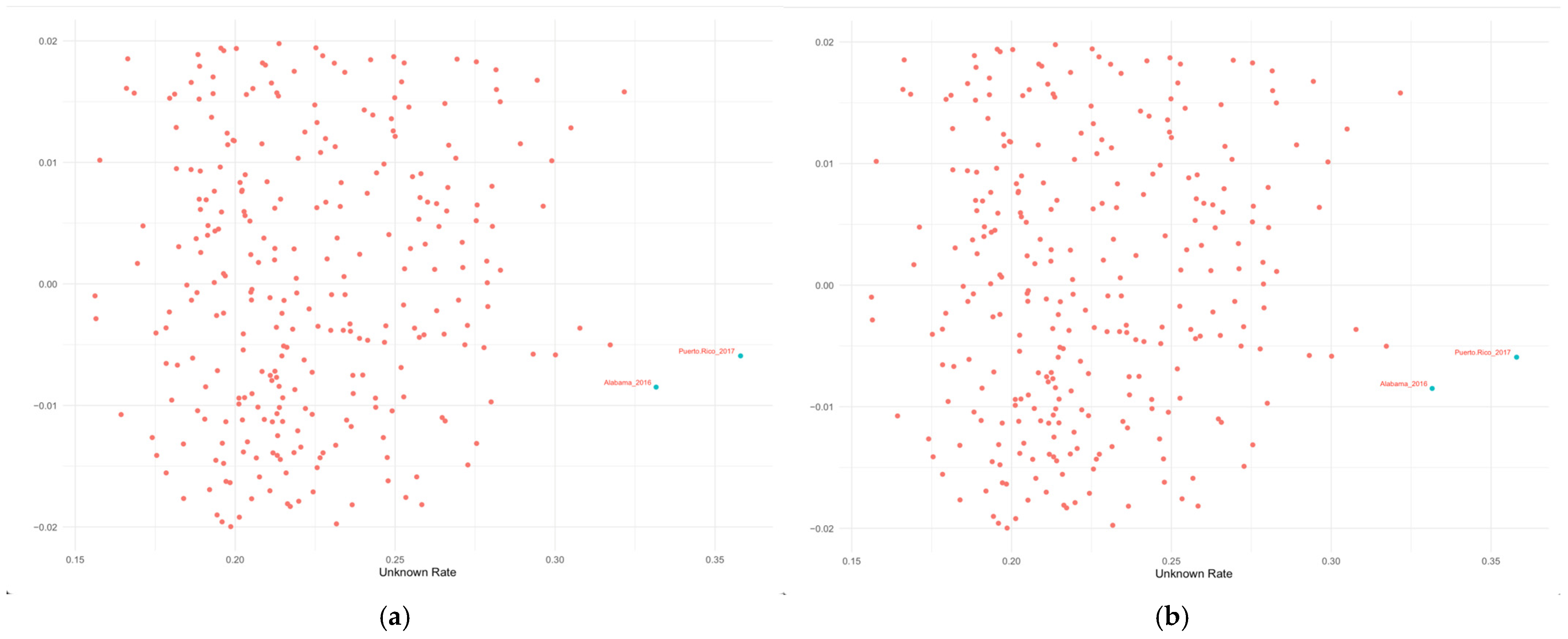
For the colorectal cancer dataset, DTOD flagged several registry years with exceptionally high proportions of unknown tumor size. Notable examples, such as Puerto Rico in 2017 and Alabama in 2016 (

Table 2. Registry-year observations flagged as outliers in the unknown tumor size rate for colorectal cancer by five detection methods (DTOD, Modified Z-score, IQR, Z-score, and kNN).

Methods	Outliers Detected
DTOD	Alabama_2016, Puerto.Rico_2017
Modified Z-score	Puerto.Rico_2017
IQR	Alabama_2016, Puerto.Rico_2017
Z-score	Puerto.Rico_2017
kNN	Puerto.Rico_2017

), were distinct from the majority of registry years, which were concentrated at lower values.

A sensitivity analysis confirmed that the outliers identified by DTOD were consistently located at the edges of the distribution in scatter plots, separate from the main cluster of registry-year observations. This pattern is demonstrated in Figure 1a, which shows the flagged points, such as Alabama 2016 and Puerto Rico 2017, as clear deviations in the upper tail. Additionally, Figure 1b highlights the outliers found exclusively by DTOD.

The credibility of DTOD’s findings was reinforced by the significant overlap with outliers identified by conventional methods, such as the IQR and the Modified Z-score (Table 2). However, DTOD also demonstrated greater sensitivity, capturing additional marginal outliers that symmetric cut-off methods did not identify, as illustrated in Figure 1b.

3.4.2. Lung Cancer Results (High Skewness)

The lung cancer dataset comprises data from 57 U.S. cancer registries for 2016–2020, yielding 285 registry-year observations of the unknown tumor size rate. This dataset exhibits skewness of 1.899, which, although below 2, is classified as high skewness. Consequently, the analysis uses outlier-detection thresholds specifically designed for highly skewed distributions to enhance the robustness of the DTOD method.

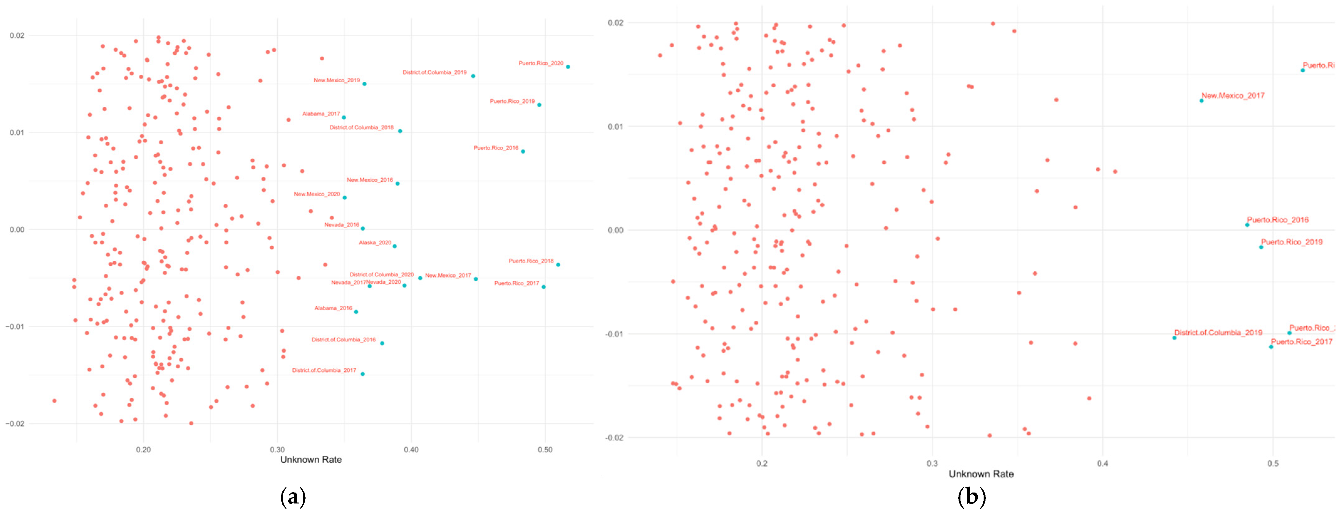
For the lung cancer dataset, DTOD flagged multiple registry years with exceptionally high proportions of unknown tumor size. Notable examples, such as the District of Columbia in 2019 and Puerto Rico across several consecutive years from 2016 to 2020 (

Table 3. Registry-year observations flagged as outliers in the unknown tumor size rate for lung cancer by five detection methods (DTOD, Modified Z-score, IQR, Z-score, and kNN).

Methods	Outliers Detected
DTOD	District.of.Columbia_2019, New.Mexico_2017, Puerto.Rico_2016, Puerto.Rico_2017, Puerto.Rico_2018, Puerto.Rico_2019, Puerto.Rico_2020
Modified Z-score	Alabama_2016, Alabama_2017, Alaska_2020, District.of.Columbia_2016, District.of.Columbia_2017, District.of.Columbia_2018, District.of.Columbia_2019, District.of.Columbia_2020, Nevada_2016, Nevada_2017, Nevada_2020, New.Mexico_2016, New.Mexico_2017, New.Mexico_2018, New.Mexico_2019, New.Mexico_2020, Puerto.Rico_2016, Puerto.Rico_2017
IQR	Alabama_2016, Alaska_2020, District.of.Columbia_2016, District.of.Columbia_2017, District.of.Columbia_2018, District.of.Columbia_2019, District.of.Columbia_2020, Nevada_2016, Nevada_2017, Nevada_2020, New.Mexico_2016, New.Mexico_2017, New.Mexico_2018, New.Mexico_2019, New.Mexico_2020, Puerto.Rico_2016, Puerto.Rico_2017, Puerto.Rico_2018
Z-score	New.Mexico_2017, Puerto.Rico_2016, Puerto.Rico_2017, Puerto.Rico_2018, Puerto.Rico_2019, Puerto.Rico_2020
kNN	Puerto.Rico_2020

), were positioned at the extreme right tail of the distribution, standing out even within an overall high-value range. As shown in Table 3, many of these DTOD-identified outliers were also corroborated by other detection methods.

DTOD’s robustness was confirmed by the location of the outliers it flagged. As shown in Figure 2a, these outliers were situated exclusively in the extreme right tail, distinctly separate from the central cluster of registry-year data. Additionally, Figure 2b highlights the outliers detected solely by DTOD, emphasizing its ability to reduce the false positives often generated by symmetric methods.

4. Discussion

The current design and testing of the DTOD are primarily based on right-skewed distributions. Experimental results indicate that the method performs especially well under both light- and high-skewness conditions. However, consistent with the observed results, sensitivity is relatively moderate under middle-skewness scenarios. Methodologically, this suggests that distributions with moderate asymmetry exhibit a “transitional” tail morphology, in which the boundary between the underlying distribution and contaminated points is less distinct. In such cases, the probabilistic trimming stage may be less decisive, suggesting that detection ability could benefit from further optimization by fine-tuning the adjustment strategy for thresholds $t_1$ and $t_2$ specifically within these transitional ranges.

Another challenge lies in reliably estimating the shape and scale parameters of the data distribution. While the current use of the MASS package for Gamma fitting works well for positive data, it has limitations when dealing with negative values. Furthermore, in simulation, we manually computed the shape and scale parameters using the formulas, yielding estimates comparable to those obtained with the formulas; however, further improvement is still possible. Our results demonstrate that the iterative trimming stage stabilizes these estimates; however, future enhancements using more robust fitting techniques, such as M-estimation or L-moments, could further improve the method’s generalization and performance in noisier datasets.

While the simulation performed in this study utilizes normal contamination at the extreme quantiles to establish a controlled baseline for performance evaluation, the underlying data-generating distributions in our simulations were primarily right-skewed and unimodal, aligning closely with the assumptions of DTOD. Because DTOD removes potential outliers via a probabilistic trimming mechanism guided by the fitted distribution, the method retains robustness even when the true distribution deviates only moderately from the Gamma family. Nonetheless, the efficiency of the tail-based adjustments may change under symmetric, multimodal, or centrally contaminated structures, and these scenarios should be examined more thoroughly in future work. We acknowledge that real-world anomalies often follow more complex mixture models or heavy-tailed distributions. This setup serves as a foundational assessment of the DTOD’s sensitivity, with future work intended to explore varying contamination rates and diverse mixture regimes to further stress-test the algorithm’s robustness.

Although the effectiveness of the DTOD has been demonstrated under skewed distributions, particularly right-skewed Gamma-like structures, future research should aim to extend its applicability and generalizability to left-skewed distributions and alternative bounded models. For the NAACCR applied example, the Gamma framework was utilized to capture the pronounced right-skewness of ‘unknown’ tumor size reporting rates. While these are technically bounded proportions [0, 1], the observed mean rates are significantly low (typically < 0.10), where the Gamma distribution provides a computationally efficient and robust approximation of the tail behavior. Future iterations should incorporate Beta distributions or Logit-Normal models to provide a theoretically rigorous treatment of proportions that approach the upper boundary, accounting for the complexities of real-world data.

For statistical testing of each observation, the current implementation uses the BH procedure to control the FDR. While we acknowledge that registry-year data may exhibit temporal dependence, the BH method is generally robust under positive regression dependency. Given the conservative behavior of the DTOD in identifying high-confidence outliers, the potential for mild FDR inflation is expected to be minimal. Future iterations of the algorithm could incorporate the Benjamini—Yekutieli (BY) adjustment to provide stricter control in cases of more complex dependence structures.

5. Conclusions

This study reframes an adaptive outlier detection method (DTOD), designed explicitly for skewed distributions, to address the limitations of traditional techniques that assume normality or symmetry. The framework integrates a two-stage process: first, probabilistic trimming uses initial distribution fitting and weighted adjustments to mitigate the influence of extreme values; second, skewness-guided thresholding dynamically establishes asymmetric thresholds, denoted as $t_1$ and $t_2$, to form an adaptive detection interval. This design allows for a sophisticated balance between robustness and sensitivity, ensuring the model adapts to the data’s inherent asymmetry rather than distorting it.

Validation through large-scale simulation experiments across light-, middle-, and high-skewness levels confirms the method’s versatility. The DTOD is particularly effective at both ends of the spectrum: enhancing sensitivity for detecting subtle anomalies in light-skewed data while serving as a conservative, high-confidence screening tool that controls false positives in highly skewed environments. These findings were further corroborated by real-world applications. In a colorectal cancer dataset characterized by light skewness, the method successfully identified outliers with abnormally high rates of unknown tumor size; conversely, in a highly skewed lung cancer dataset, it maintained a low misclassification rate by effectively distinguishing marginal points from true anomalies. Ultimately, the DTOD provides a promising, interpretable solution for improving data quality in univariate skewed scenarios, with future research aimed at extending its application to left-skewed, mixture, multivariate, and nonparametric distributions.

References

- Koch, A.L. The logarithm in biology 1. Mechanisms generating the log-normal distribution exactly. J. Theor. Biol. 1966, 12, 276–290. [Google Scholar] [CrossRef] [Scilit] [PubMed]
- Limpert, E.; Stahel, W.A.; Abbt, M. Log-normal distributions across the sciences: Keys and clues: On the charms of statistics, and how mechanical models resembling gambling machines offer a link to a handy way to characterize log-normal distributions, which can provide deeper insight into variability and probability—Normal or log-normal: That is the question. BioScience 2001, 51, 341–352. [Google Scholar]
- Sartwell, P.E. The Distribution of Incubation Periods of Infectious Diseases. Am. J. Hyg. 1950, 51, 310–318. [Google Scholar] [PubMed]
- Yaro, A.S.; Maly, F.; Prazak, P. Outlier Detection in Time-Series Receive Signal Strength Observation Using Z-Score Method with Sn Scale Estimator for Indoor Localization. Appl. Sci. 2023, 13, 3900. [Google Scholar] [CrossRef] [Scilit]
- Miller, J.N.; Comm, A.M. Using the Grubbs and Cochran tests to identify outliers. Anal. Methods 2015, 7, 7948–7950. [Google Scholar] [CrossRef] [Scilit]
- Ott, W.R. Environmental Statistics and Data Analysis; Routledge: Oxfordshire, UK, 2018. [Google Scholar]
- Bantis, L.E.; Nakas, C.T.; Reiser, B. Construction of confidence regions in the ROC space after the estimation of the optimal Youden index-based cut-off point. Biometrics 2014, 70, 212–223. [Google Scholar] [CrossRef] [Scilit]
- Leys, C.; Ley, C.; Klein, O.; Bernard, P.; Licata, L. Detecting outliers: Do not use standard deviation around the mean, use absolute deviation around the median. J. Exp. Soc. Psychol. 2013, 49, 764–766. [Google Scholar] [CrossRef] [Scilit]
- Hubert, M.; Vandervieren, E. An adjusted boxplot for skewed distributions. Comput. Stat. Data Anal. 2008, 52, 5186–5201. [Google Scholar] [CrossRef] [Scilit]
- Brys, G.; Hubert, M.; Struyf, A. A robust measure of skewness. J. Comput. Graph. Stat. 2004, 13, 996–1017. [Google Scholar] [CrossRef] [Scilit]
- Wang, L.Z.; Zou, L.K. Research on algorithms for mining distance-based outliers. Chin. J. Electron. 2005, 14, 485–490. [Google Scholar]
- Yoon, S.; Kim, S.S.; Chae, S.H.; Park, N.S. Introducing new outlier detection method using robust statistical distance in water quality data. Desalin. Water Treat. 2019, 149, 157–163. [Google Scholar] [CrossRef] [Scilit]
- Penny, K.I. Appropriate critical values when testing for a single multivariate outlier by using the Mahalanobis distance. Appl. Stat. J. R. St. C 1996, 45, 73–81. [Google Scholar] [CrossRef] [Scilit]
- Cabana, E.; Lillo, R.E.; Laniado, H. Multivariate outlier detection based on a robust Mahalanobis distance with shrinkage estimators. Stat. Pap. 2021, 62, 1583–1609. [Google Scholar] [CrossRef] [Scilit]
- Alsini, R.; Almakrab, A.; Ibrahim, A.; Ma, X.G. Improving the outlier detection method in concrete mix design by combining the isolation forest and local outlier factor. Constr. Build. Mater. 2021, 270, 121396. [Google Scholar] [CrossRef] [Scilit]
- Heigl, M.; Anand, K.A.; Urmann, A.; Fiala, D.; Schramm, M.; Hable, R. On the Improvement of the Isolation Forest Algorithm for Outlier Detection with Streaming Data. Electronics 2021, 10, 1534. [Google Scholar] [CrossRef] [Scilit]
- Binetti, M.S.; Uricchio, V.F.; Massarelli, C. Isolation Forest for Environmental Monitoring: A Data-Driven Approach to Land Management. Environments 2025, 12, 116. [Google Scholar] [CrossRef] [Scilit]
- Chaabouni, A.; Boujelben, M.A. Outlier Ensemble Based on Isolation Forest: The CBOEA Approach. Found. Comput. Decis. S 2025, 50, 27–55. [Google Scholar] [CrossRef] [Scilit]
- Erfani, S.M.; Rajasegarar, S.; Karunasekera, S.; Leckie, C. High-dimensional and large-scale anomaly detection using a linear one-class SVM with deep learning. Pattern Recognit. 2016, 58, 121–134. [Google Scholar] [CrossRef] [Scilit]
- O’Neill, H.; Khalid, Y.; Spink, G.; Thorpe, P. A one-class support vector machine for detecting valve stiction. Digit. Chem. Eng. 2023, 8, 100116. [Google Scholar] [CrossRef] [Scilit]
- Zhao, X.X.; Tian, Y.J.; Zheng, C.H. Robust one-class support vector machine. Neural Netw. 2025, 188, 107416. [Google Scholar] [CrossRef] [Scilit]
- Hubert, M.; Rousseeuw, P.; Verdonck, T. Robust PCA for skewed data and its outlier map. Comput. Stat. Data 2009, 53, 2264–2274. [Google Scholar] [CrossRef] [Scilit]
- Jackson, D.A.; Chen, Y. Robust principal component analysis and outlier detection with ecological data. Environmetrics 2004, 15, 129–139. [Google Scholar] [CrossRef] [Scilit]
- Fowler, J.W.; Alpert, B.K.; Joe, Y.I.; O’Neil, G.C.; Swetz, D.S.; Ullom, J.N. A Robust Principal Component Analysis for Outlier Identification in Messy Microcalorimeter Data. J. Low Temp. Phys. 2020, 199, 745–753. [Google Scholar] [CrossRef] [Scilit] [PubMed]
- Nakayama, Y.; Yata, K.; Aoshima, M. Test for high-dimensional outliers with principal component analysis. Jpn. J. Stat. Data Sci. 2024, 7, 739–766. [Google Scholar] [CrossRef] [Scilit]
- Pang, G.S.; Shen, C.H.; Cao, L.B.; Van den Hengel, A. Deep Learning for Anomaly Detection: A Review. ACM Comput. Surv. 2021, 54, 38. [Google Scholar] [CrossRef] [Scilit]
- Gkountakos, K.; Ioannidis, K.; Demestichas, K.; Vrochidis, S.; Kompatsiaris, I. A Comprehensive Review of Deep Learning-Based Anomaly Detection Methods for Precision Agriculture. IEEE Access 2024, 12, 197715–197733. [Google Scholar] [CrossRef] [Scilit]
- Groeneveld, R.A.; Meeden, G. Measuring Skewness and Kurtosis. J. R. Stat. Soc. Ser. D Stat. 1984, 33, 391–399. [Google Scholar] [CrossRef] [Scilit]
- Doric, D.; Nikolic-Doric, E.; Jevremovic, V.; Malisic, J. On measuring skewness and kurtosis. Qual. Quant. 2009, 43, 481–493. [Google Scholar] [CrossRef] [Scilit]
- Jones, M.C.; Rosco, J.F.; Pewsey, A. Skewness-Invariant Measures of Kurtosis. Am. Stat. 2011, 65, 89–95. [Google Scholar] [CrossRef] [Scilit]
- Reinsel, G.; Craig. Introduction to Mathematical Statistics (4th ed.) by Robert V. Hogg, Allen T. Craig. J. Am. Stat. Assoc. 1980, 75, 474. [Google Scholar] [CrossRef] [Scilit]
- Glickman, M.E.; Rao, S.R.; Schultz, M.R. False discovery rate control is a recommended alternative to Bonferroni-type adjustments in health studies. J. Clin. Epidemiol. 2014, 67, 850–857. [Google Scholar] [CrossRef] [Scilit]
- Benjamini, Y.; Hochberg, Y. Controlling the False Discovery Rate—A Practical and Powerful Approach to Multiple Testing. J. R. Stat. Soc. B 1995, 57, 289–300. [Google Scholar] [CrossRef] [Scilit]