A Comprehensive Evaluation of Produced-Water Reuse Potential for Cementing Operations in the Delaware Basin

Abstract

Freshwater demand for cementing operations in the Delaware Basin continues to increase with expanding unconventional development, creating a high demand for an alternative source of water. This study develops a chemistry screening and operational framework to evaluate the reusability potential in cementing operations in the Delaware Basin. A three-tier screening system for the produced-water samples was established by using the major-ion chemistry, total dissolved solids (TDS), pH, and saturation index (SI) thresholds derived from the cement literature and American Petroleum Institute (API) guidelines. The results of the geochemical screening aid in classifying the water samples into four suitability categories: Excellent/Preferred, Good/Suitable, Moderate/Marginal, and Poor/Unsuitable. The results suggest that the samples obtained from the Loving, Pecos, Reeves, Eddy and Lea counties meet the criteria for reuse in cementing operations with minimal conditioning. To assess the feasibility of operational use, a probabilistic forecasting model was developed to predict the cement water demand in 2026 for the basin. Linear regression of historical drilling trends between 2015 and 2025 showcased that approximately 3595 new wells will be drilled, with an average well depth of 21,778 ft. To evaluate whether the produced-water volumes in the basin are adequate for reuse in cementing, a Monte Carlo simulation (10,000 iterations) estimated an annual cementing water requirement centered at 6.16 MMbbl/year (P50). Produced-water availability from wells classified as Excellent/Preferred was also modeled probabilistically, using uncertainty in the water–oil ratio (WOR), estimated ultimate recovery (EUR), and forecast duration. These results demonstrate the potential for produced-water reuse to reduce freshwater demand for cementing operations in the Delaware Basin.

1. Introduction

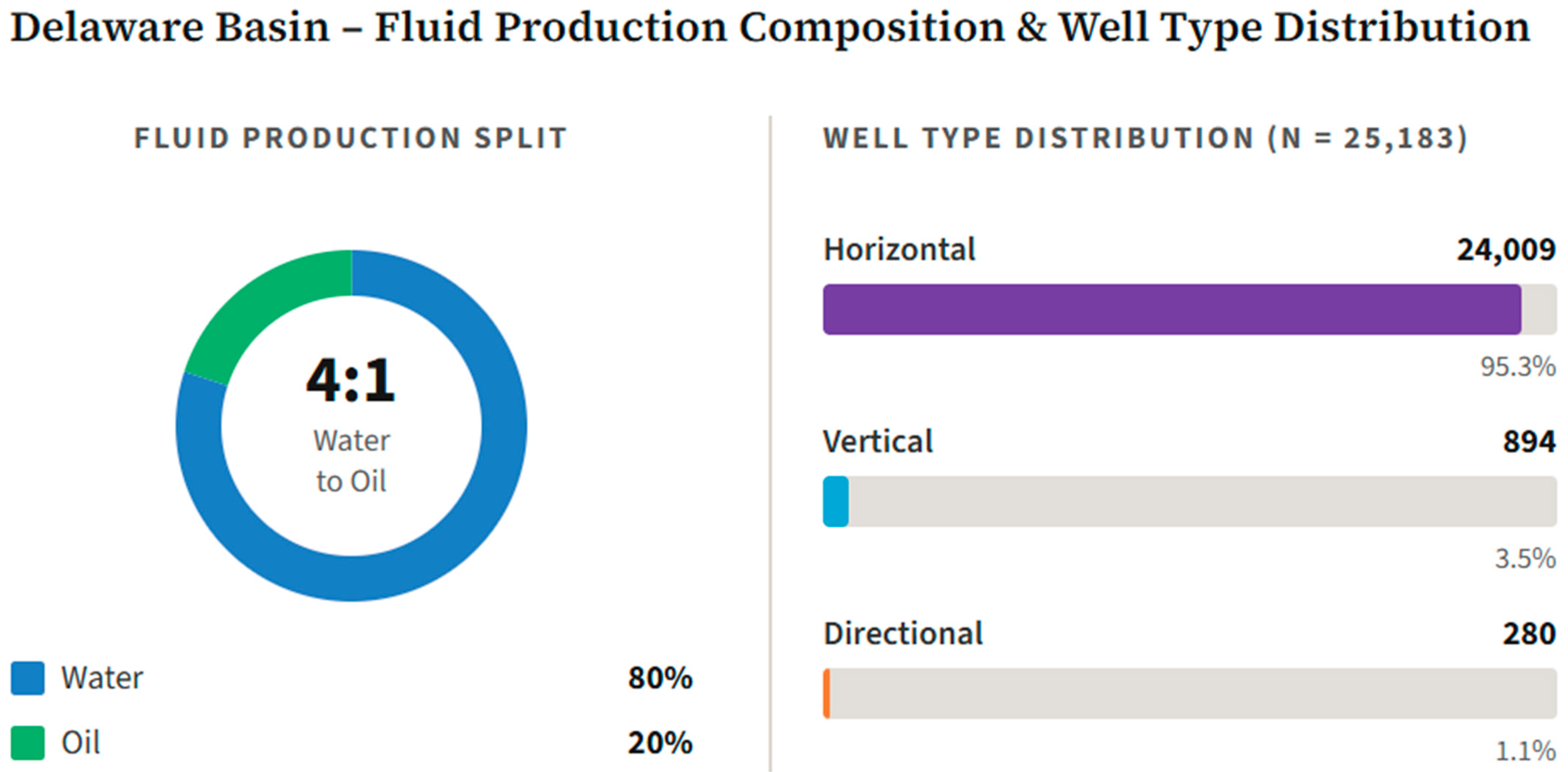
The Permian Basin generates an enormous volume of produced water, which is increasing alongside oil and gas production. Recent estimates indicate that Permian wells collectively produce approximately tens of millions of barrels of water per day. In 2019, approximately 11 million barrels per day of wastewater were generated in the Permian Basin; this figure has since increased, surpassing 15 million barrels per day by the mid-2020s [1]. Projections suggest that the region could exceed 20 million barrels of produced water per day by 2024 and continue to rise to 26–32 million barrels per day over the next decade. To put this into perspective, many Delaware Basin wells yield water-to-oil ratios of 4:1 up to 10:1, meaning that some wells produce ten barrels of water for every barrel of oil. As shown in Figure 1, by 2026, the average cumulative oil-to-cumulative water production ratio of 25,183 producing wells in the Delaware Basin is 1:4, with 95% of horizontal wells.

Figure 1. Oil and water production history in Delaware Basin: from 25,183 producing wells up to January 2026, with 27,696 wellbores, and cumulative oil production of 7.13 billion bbls and water production of 28.85 billion bbls, as of January 2026 (data from Enverus database).

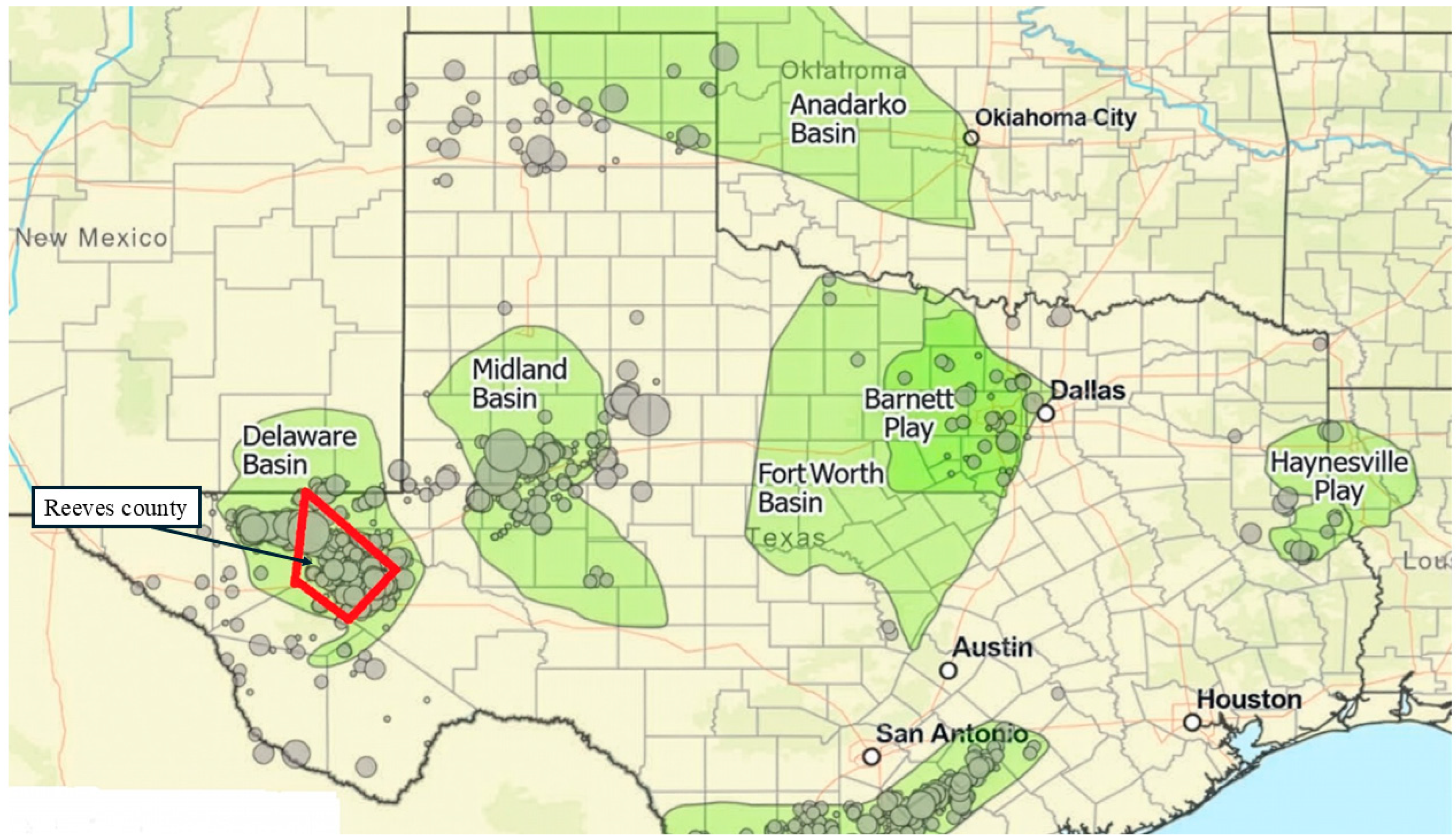
This “water tsunami” has created a chronic burden in handling and disposing of the produced water. Operators have traditionally managed produced water by injecting it into saltwater disposal (SWD) wells, pumping billions of barrels per year into subsurface formations. However, this once-routine solution is reaching its limits under geological and regulatory constraints. Similar produced-water management challenges have also been reported in other major oilfields worldwide, although the dominant bottlenecks differ by region. For example, Wang et al. (2024) [2] showed that in flooding-based oilfields, the gravitational-settling performance and sump-oil growth are strongly influenced by the oil content, daily processing capacity, polymer concentration, and suspended solids, underscoring that produced-water management is a global but field-specific challenge. In the Delaware Basin, one of the most pressing drivers is induced seismicity that is linked to massive produced-water injection. Since 2009, the Permian Basin has experienced a sharp uptick in earthquakes attributed to SWD injection [3]. In the Delaware Basin (Figure 2), large volumes of injected fluids into relatively shallow formations (e.g., the Delaware Mountain Group) have elevated subsurface pressures, thereby triggering more frequent seismic events [4]. The New Mexico Oil Conservation Division (NMOCD) imposed a moratorium on new shallow disposal in 2016, due to concerns that rising formation pressures and water flows were affecting drilling and nearby producing zones, forcing operators to shift to more costly deep disposal wells or to transport water across state lines [5]. In Texas, the Railroad Commission (RRC) responded to rising earthquake activity with stricter guidelines (e.g., in 2025) [6]. These measures and localized Seismic Response Areas are restricting water disposal, reducing operational flexibility. This creates bottlenecks: disposal well capacities are strained, trucking distances and costs rise, and wells may be curtailed if water is not managed quickly. Disposal capacity and pore space are now critical resources, making produced-water management a key operational challenge.

Figure 2. Texas seismicity since 2017. Symbol (circle) size scales with earthquake magnitude: small circles are 1, and large circles are greater than 5. The map shows the West Texas Delaware Basin, including Reeves County, where elevated seismic activity has been observed. (modified after [7]).

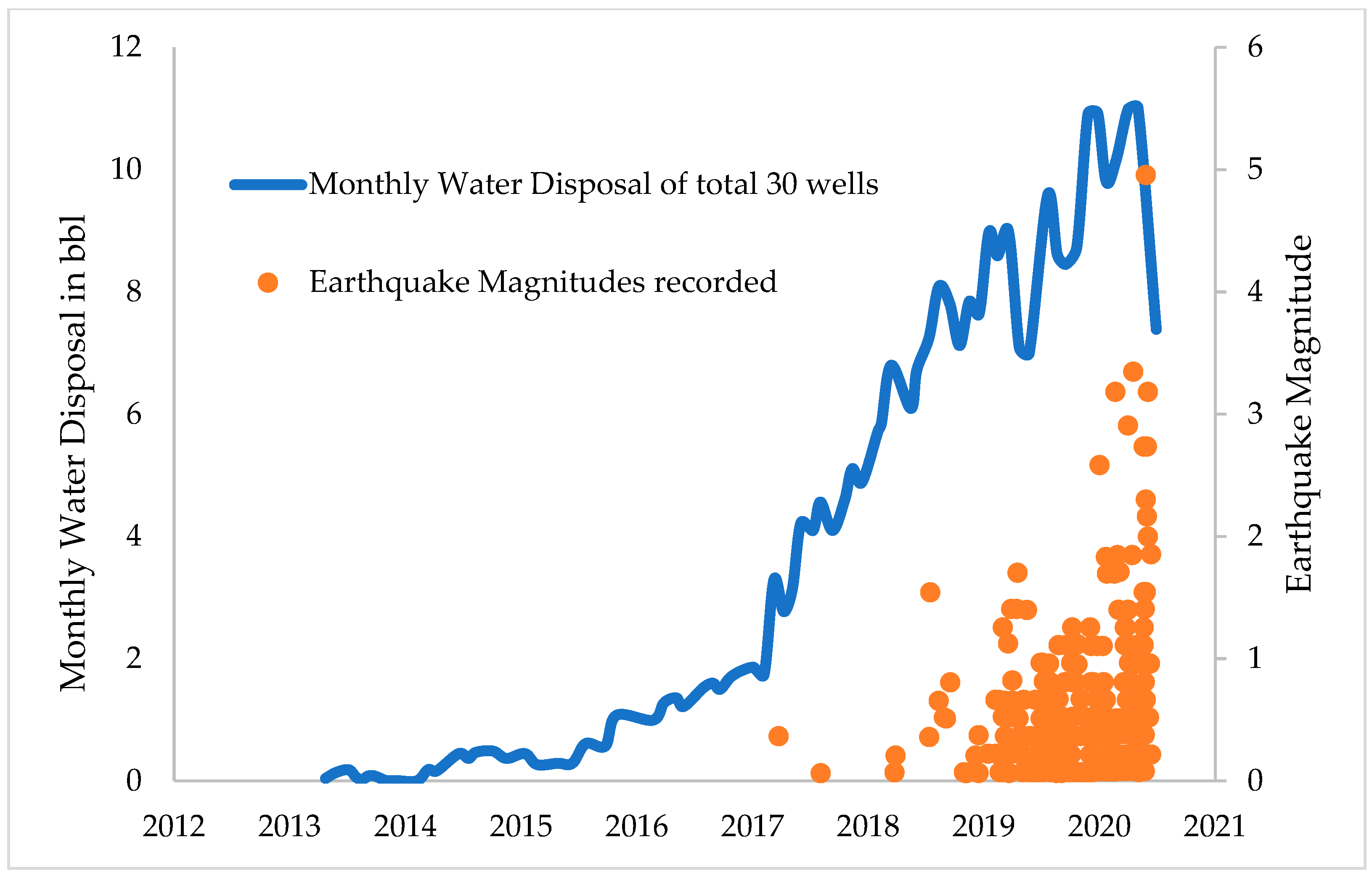
Reeves County is in West Texas and lies within the Delaware Basin (Figure 2), making it a key area for both unconventional development and produced-water management. In this region, Skoumal et al. [8] document the Mw 5.0 26 March 2020 earthquake that occurred near the Reeves–Culberson county line in the southern Delaware Basin. Figure 3 compares the monthly produced-water disposal volumes in nearby monitored SWD wells (28 shallow and 2 deep disposal wells) with the magnitudes of earthquakes above the magnitude of completeness. The figure shows that disposal volumes increased over time and that larger-magnitude events became more frequent as injection intensified, culminating in the Mw 5.0 mainshock. The authors interpret this pattern as being consistent with wastewater disposal contributing to pressure and stress changes that promoted seismicity in the area.

Figure 3. Monthly total wastewater disposal volumes of 30 wells in the region around the Mw 5.0 (Reeves County), compared with earthquake magnitudes (modified after [8]).

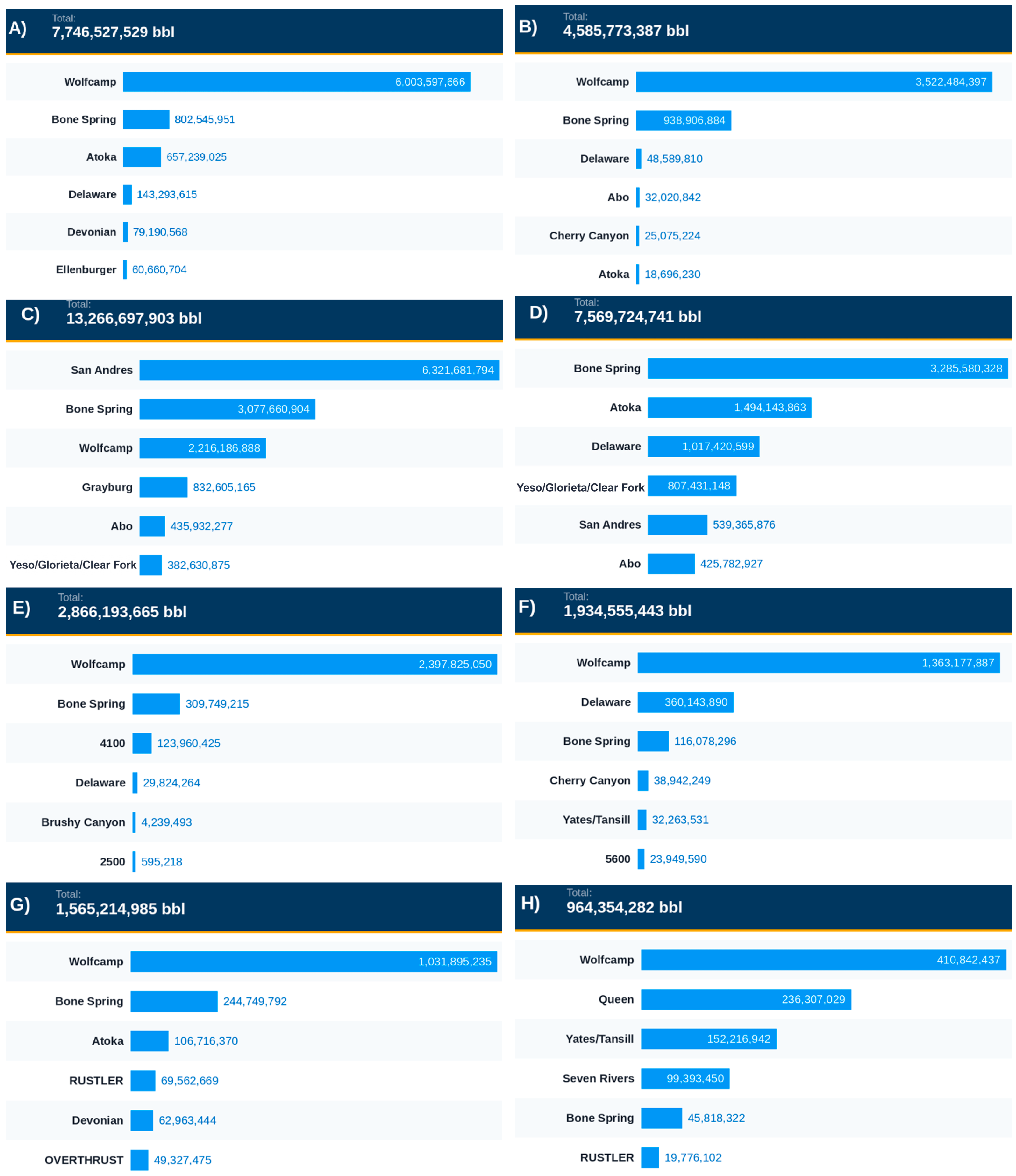
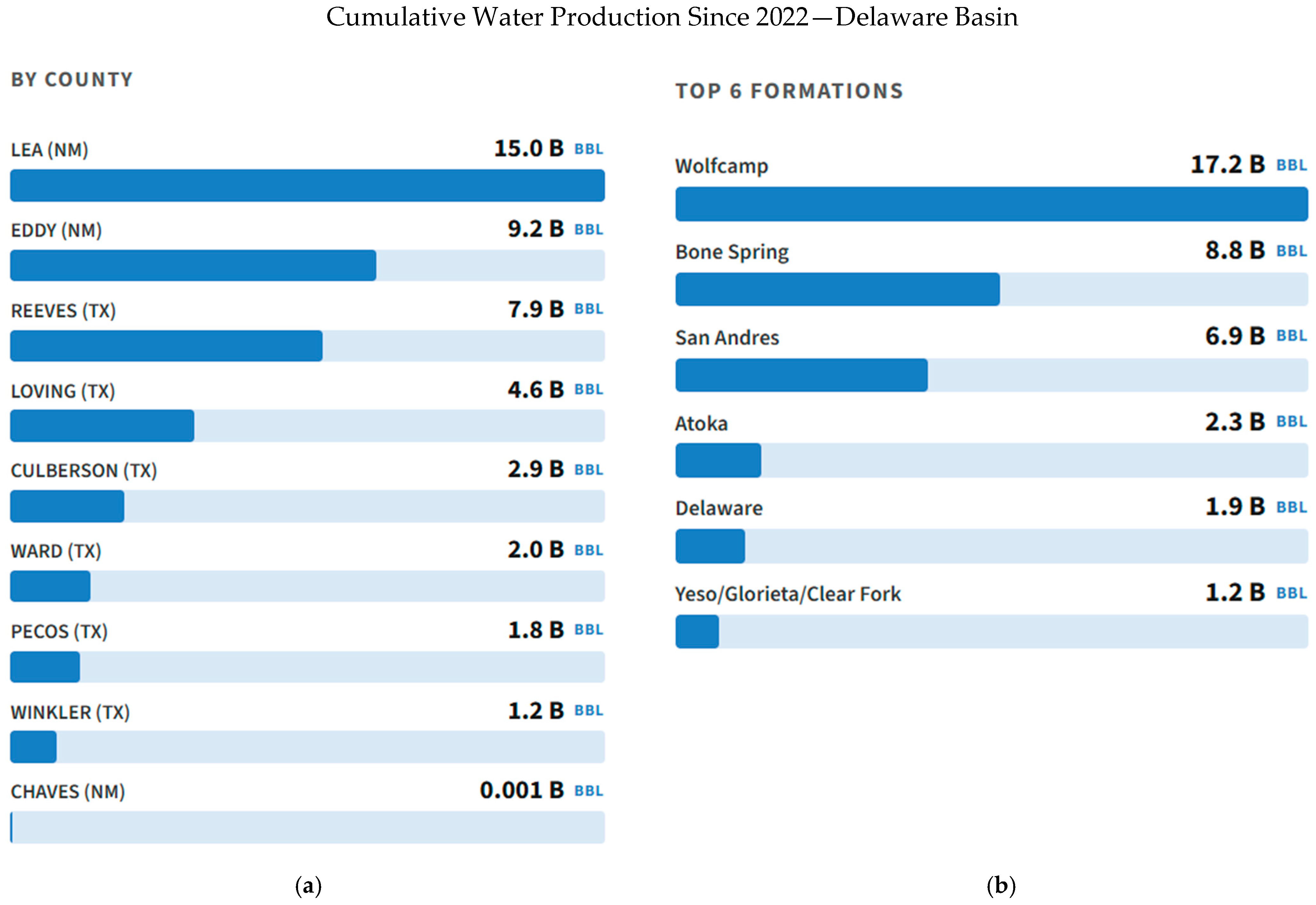
To quantify the scale and distribution of the produced water within the AoR, produced-water volumes were compiled from the Enverus database for the Delaware Basin counties evaluated in this study (Lea and Eddy in New Mexico; Reeves, Loving, Culberson, Ward, Pecos, and Winkler in Texas; with minor contribution from Chaves, NM) [9]. Figure 4 summarizes cumulative produced-water volumes since January 2022 by county and formation. Figure 4a summarizes the cumulative produced-water production by county and shows a strong spatial concentration: Lea County (NM) contributes 14.96 billion bbl, Eddy County (NM) 9.21 billion bbl, and Reeves County (TX) 7.86 billion bbl, followed by Loving (TX) (4.64 billion bbl) and Culberson (TX) (2.87 billion bbl). The remaining counties (Ward, Pecos, Winkler, and Chaves) contribute smaller but non-negligible volumes. This distribution identifies the counties where water-handling requirements are most persistent and where constraints on transport, storage, reuse, and disposal are most likely to influence the operations. At the stratigraphic scale, Figure 4b ranks the highest-producing formations by cumulative produced-water volume since 2022 across the full study area. The Wolfcamp interval is the dominant contributor (17.17 billion bbl), followed by Bone Spring (8.82 billion bbl) and San Andres (6.86 billion bbl). Together, these three units account for most of the produced water captured in the dataset, indicating that both unconventional development (Wolfcamp and Bone Spring) and legacy/stacked conventional intervals (San Andres) jointly govern the produced-water volumes in the Delaware Basin region. Appendix A Figure A1 breaks down the water totals by formation within eight key counties, highlighting differences in local water sources. For example, Wolfcamp dominates in some West Texas counties, while Lea County shows a mix of San Andres, Bone Spring, and Wolfcamp, indicating different development focuses and reservoir availability. This helps us to anticipate variability in water chemistry and treatment needs, guiding reuse strategies.

Figure 4. Produced-water production in the Delaware Basin study area since 2022 (Enverus). (a) Cumulative produced-water production by county. (b) Top producing formations by cumulative produced-water production.

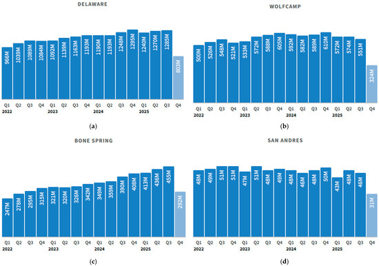
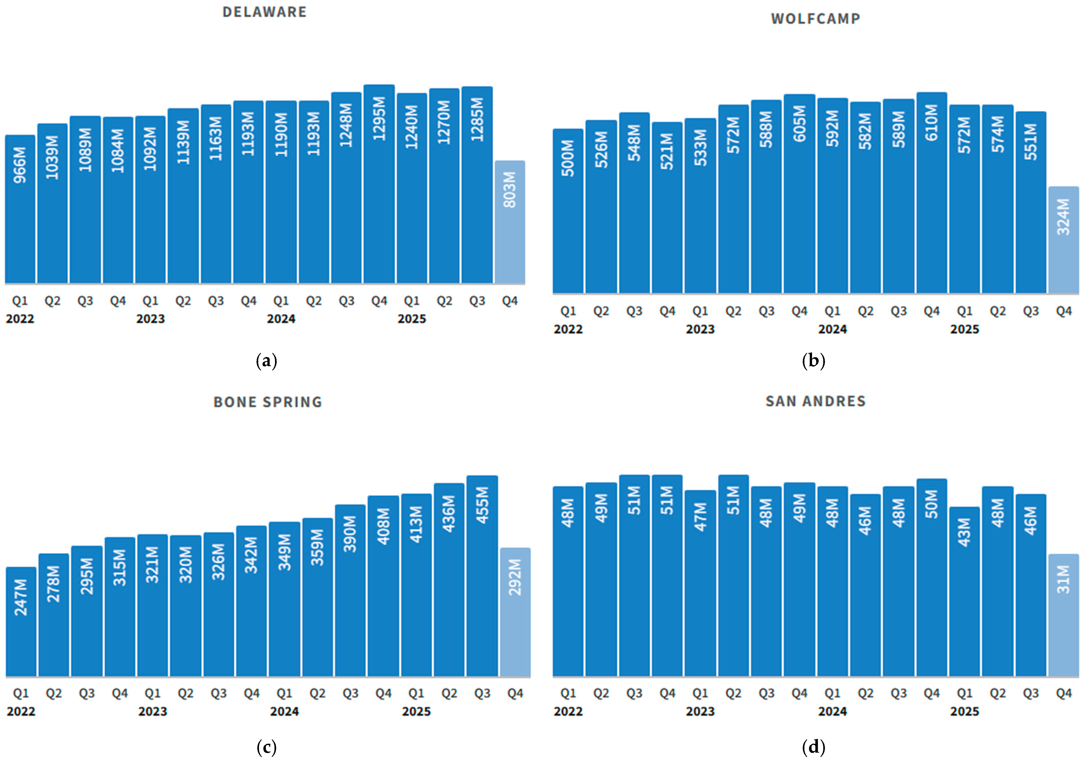
Finally, recent temporal behavior is summarized in Figure 5, which reports quarterly produced-water volumes since 2022 for the study area and for the dominant contributing formations. The total produced-water volumes increase from approximately 0.97 billion bbl per quarter in early 2022 to approximately 1.25–1.28 billion bbl per quarter by 2024–2025, indicating sustained high water generation in the Delaware Basin. Over the same period, Wolfcamp and Bone Spring remain the primary drivers of basin-wide produced-water volumes, while San Andres contributes a smaller but persistent baseline.

Figure 5. Quarterly produced-water volumes in the Delaware Basin study area since 2022 (Enverus). (a) Total produced-water volume aggregated across the study area. (b) Wolfcamp produced-water volume. (c) Bone Spring produced-water volume. (d) San Andres produced-water volume.

Together, Figure 4, Figure 5 and Figure 6 establish the spatial, stratigraphic, and temporal “supply-side” foundation used in this study to evaluate the extent to which produced water could be treated and redirected to cementing operations in newly drilled wells across the Delaware Basin, given the region’s high drilling activity. Cementing a well is one of the most critical operations in well completion [10], which is required to secure the casing to the formation wall or previous casing strings [11]. Moreover, cement acts as a barrier between the well and the surface [12,13], isolates the formation and subsurface aquifers [14], and supports casing strings and prevents well control issues [15]. Cement slurries are designed based on the specific formation, its conditions, and characteristics, including its pressure, temperature, and chemical composition [16]. There are several types of cementing jobs, such as primary cementing, secondary cementing, cement plug, squeeze cementing, and inner string cementing [17], making the cement slurry quality of utmost importance. Cement quality largely depends on its design, including the quality and quantity of the three components of the slurry: cement, water, and the various additives [18]. There are many different additives; for example, bentonite and microsilica are employed to enhance the suspension properties of the slurries [19], sugar cane fiber is used to improve fluid loss [20], and synthetic polymer additives are used to enhance fluid loss and act as both a dispersant and retarder [21], each with their specific water contents.

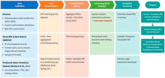
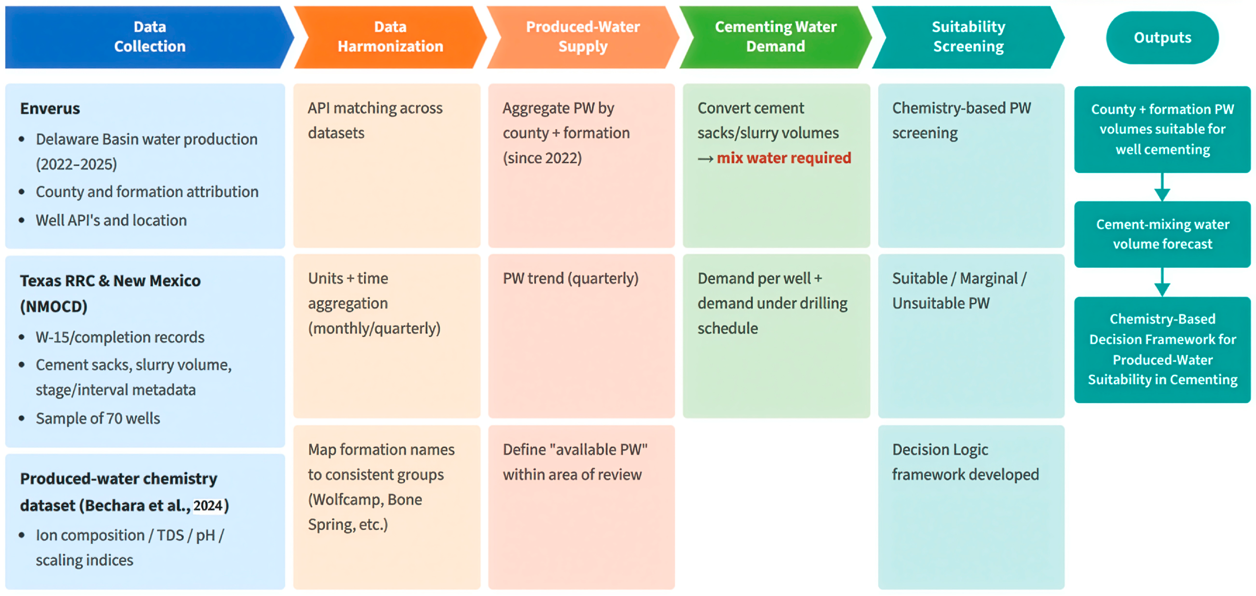
Figure 6. Workflow for estimating produced-water availability and identifying cement-mixing reuse candidates [22].

This paper introduces a basin-wide framework in the Delaware Basin for evaluating produced-water reuse in wellbore cementing operations, which remains a largely unexplored subject compared to the reuse of water in hydraulic fracturing projects. The novelty lies in incorporating a three-tier water chemistry screening system with a suitability matrix. Historical data are used to predict the basin water demand for the expected cementing operations in 2026. The combination of the water sample evaluation system and water demand prediction aids in determining whether the reuse of produced water in cementing is a viable option.

2. Methodology

2.1. Data Compilation and Preprocessing

The chemistry data for this study were collected from a previously published paper by Bechara et al. [22] in 2024, which reported the laboratory testing results for major ions, salinity, pH, and total dissolved solids, aiding in the development of the screening and classification framework discussed later in the Methodology section [22]. The casing and cementing data used in the future well-development predictions were retrieved from the Railroad Commission of Texas (RRC) and the New Mexico Oil Conservation Division (NMOCD) online databases for 70 disposal and production wells selected through stratified sampling, based on the proportional distribution of operators within each county across the Delaware Basin [23,24]. Moreover, the production and well data presented in this paper were obtained from Enverus [9]. A complete workflow is represented in Figure 6.

Although this study applies the methodology to produced-water samples in the Delaware Basin specifically, the framework was designed to be replicable in other parts of the world. The process can be customized to any field or basin through the incorporation of locally obtained chemistry, drilling, and water production data. It is not exclusive to the Delaware Basin.

2.2. Chemistry-Based Screening Framework

Prior to operational use, the produced water is analyzed based on its physicochemical properties. It begins with a data quality check before interpreting the results. For example, if the sample tested has low total dissolved solids (TDS) and high specific gravity (SG), it indicates an error in the laboratory or unit conversions, as SG directly correlates with the dissolved salt concentration in the water [1]. Moreover, the sample source must be verified to determine whether it is from the wellhead, tubing, separator, or storage, as factors such as oxygen exposure, pressure changes, and contamination can significantly affect the original water quality.

To evaluate the reuse potential of the produced water in cementing operations, a three-tier risk-based screening system was developed. The process prioritizes the parameters that are most critical to cement slurry performance and integrity. Tier 1 (Critical—Disqualifying Parameters) includes the parameters that cause cement failure. Extreme acidity or alkalinity (pH < 4 or >12) can change cement hydration behavior, which prevents setting or, in some cases, causes flash setting [25,26]. Excessive salinity from high TDS (>150,000 mg/L) can delay hydration, reduce compressive strength development, and cause issues with fluid loss control [26]. Moreover, high levels of chlorides (>80,000 mg/L), sulfates (>5000 mg/L), and magnesium (>5000 mg/L) alter the setting time and cause sulfate attack and corrosion of the casing [27,28,29]. Similarly, dissolved O₂ levels above 10 mg/L at surface conditions accelerate the corrosion of the casing strings [30].

Tier 2 (Major—Performance-Modifying Parameters) includes parameters that can significantly affect the cement slurry design and its performance. Such modifying parameters include the hardness of CaCO₃ at elevated concentrations (>5000 mg/L), which can lead to premature coagulation with anionic polymer additives; elevated sodium (Na+) (>50,000 mg/L) and bicarbonate (${\mathrm{H}\mathrm{C}\mathrm{O}}_3^{-}$)(>1500 mg/L) levels can cause retardation and overall erratic thickening times [31,32,33]. Although the parameters in this tier do not preclude reuse of the PW, they require reformulation of the cement slurry with additives such as dispersants, accelerators, or retarders.

The last tier, Tier 3 (Indicators of Scaling), parameters are diagnostic indicators that evaluate the scaling tendencies of PW. Scaling is an important consideration, as it can clog the mix equipment and negatively affect the cement permeability. Tier 3 relies heavily on saturation index (SI) calculations to evaluate whether certain minerals in water are likely to precipitate under specified temperature and pressure conditions. A nonzero SI value (SI > 0) indicates supersaturation of the water with respect to the mineral getting tested and is likely to form scale [34]. For example, an SI value for calcite greater than 0.5 may cause calcium carbonate precipitation when pH rises during cement hydration [35]. Rapid CaCO₃ scaling can significantly disrupt the cementing performance by increasing the slurry viscosity and causing unpredictable changes in the thickening time, which complicates pumping operations [36]. It may also lead to the premature plugging of pores or perforations, which can restrict fluid movement and impair proper slurry distribution [36]. High SI values for barite and gypsum (both >0.5) can precipitate sulfate-based scaling, such as BaSO₄ and CaSO₄, causing damage to equipment and hardware with which it comes into contact [37]. It is important to note that a positive SI value does not disqualify the PW completely; it does, however, indicate a risk of interference [38]. The solution to this problem is pretreatment to reduce mineral volumes.

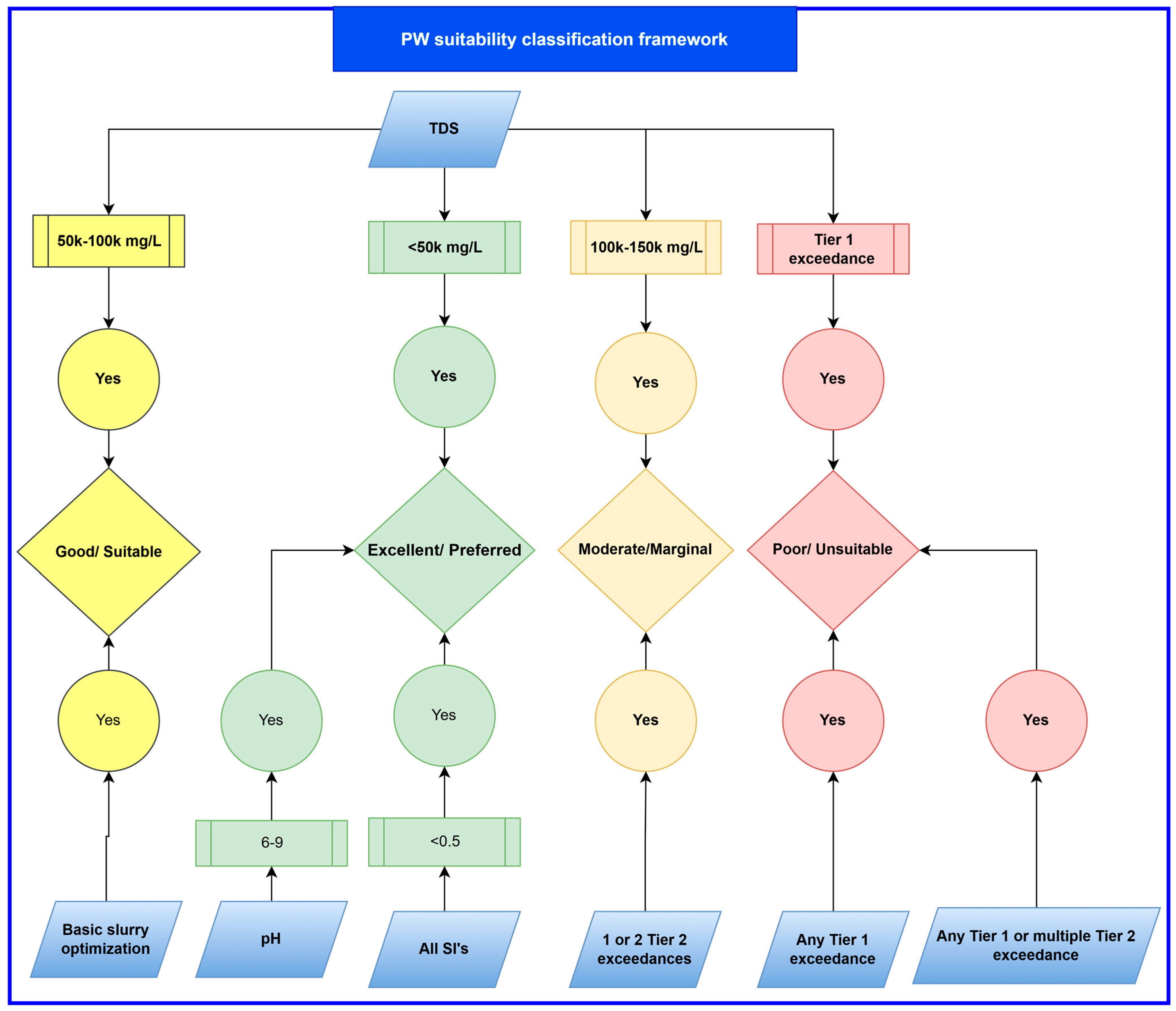
A four-class suitability matrix was developed to integrate the three-tier screening system into a tool to aid in determining which samples are best suited for cementing operations (see Figure 7).

Figure 7. Produced-water suitability decision framework.

The water samples that meet all Tier 1 limits, stay within Tier 2 (Performance-Modifying) ranges, and have a saturation index (SI) below 0.5 are classified as Excellent/Preferred, which includes a TDS < 50,000 mg/L and pH between 6 and 9. These waters can typically be used without treatment. Samples with moderate salinity levels, between 50,000 and 100,000 mg/L, and that have no critical exceedances of Tiers 1 and 2 parameters, fall into the Good/Suitable category. Good/Suitable samples may only require minor slurry optimization through additives when used in cement slurry formulation. Moreover, water samples with one or two Tier 2 (Performance-Modifying) exceedances and higher salinity levels (approximately 100,000–150,000 mg/L) are considered Moderate/Marginal, according to the system. Reuse of Moderate/Marginal water samples can be achieved after chemical conditioning to reduce TDS and other impurities. Lastly, any Tier 1 exceedance or multiple Tier 2 exceedances place the water sample in the Poor/Unsuitable category, due to the elevated risk of slurry instability, delayed hydration, or poor cement integrity. Overall, this matrix bridges the gap between geochemical analysis and real-world engineering decisions regarding the reuse of produced water in cementing operations.

The classification criteria associated with the chemical compound thresholds are developed based on the prior established literature on cement chemistry, such as Cement Chemistry by H. F. W. Taylor and Cementing by Dwight K. Smith, as well as the American Petroleum Institute-recommended practices, such as API Recommended Practice 10B-2: Recommended Practice for Testing Well Cements [39,40]. Moreover, the thresholds for the saturation indices were based on geochemical modeling principles, as outlined by David L. Parkhurst and C.A.J. Appelo [41].

Future annual produced-water availability from 202 high-quality wells was estimated using probabilistic simulation. The cumulative water was calculated as follows:

$$Water=WOR\times EUR Oil$$

and annualized using the forecast duration. Variability of ±20% (WOR), ±15% (EUR), and ±10% (forecast months) was incorporated through Monte Carlo simulation (10,000 iterations) to generate a distribution of the annual water availability.

2.3. Cementing Water Demand Forecast

While the preceding section establishes a working system that decides whether a water sample is suitable to be reused in cementing based on its chemical composition and how much future water will be produced based on that categorization, the practical implementation depends upon operational demands. Therefore, the second part of the methodology focuses on developing a process to predict water demand for cementing in the Delaware Basin in 2026.

To estimate the total water demand for cementing operations in the Delaware basin in 2026, a comprehensive forecasting system for the entire basin was developed. The total water demand was determined as a product of three main components: the predicted number of wells to be drilled, the predicted average depth of those wells and the predicted water required per foot of well. To predict the number of wells, historical well header data across the basin were analyzed to determine trends based on operating patterns such as the frequency of wells drilled, the geographical location, and overall rig development strategies. The average well depth was predicted by examining the same basin-wide dataset to evaluate the wells based on vertical and lateral depth targets, which allows for accuracy and representativeness in the results. Finally, a stratified sample of the entire Delaware basin was taken to make a representative estimate of the water volume required per foot of well depth. Stratified sampling ensures that samples are drawn from non-overlapping strata to avoid bias toward more populous subsets of wells developed in the basin.

Due to the uncertainties that naturally arise from predicting future trends, 10,000 Monte Carlo simulations were conducted to incorporate such uncertainties into the calculations. The estimated water requirement of wells may not be representative of the entire basin; therefore, the results were normalized per foot depth to ensure better accuracy. Moreover, to account for worst-case scenarios, the upper bound of the results was used.

First, a simple linear regression was developed to predict the number of drilled wells and the average depth of the wells in the Delaware Basin for the year of 2026. To fit the regression model, historical data from 2015 to 2025 were used to capture the evolving model of the quantity of wells and their respective depth trends in the Delaware basin.

Then, after obtaining future predictions for the number of wells and average depth, we moved onto estimating the water requirement for the cementing operations, accordingly. To explain, the water volume was first calculated for each casing string, then added together for all the casing strings in the well. The equation used to calculate the water volume in barrels is as follows.

$$V_{water}\left(bbl\right)={\displaystyle \frac{V_{slurry }-V_{cement}}{5.61458}}$$

(1)

$$V_{slurry }=Cement Yiled\ast Cement Volume$$

(2)

It is important to note that the volume of additives added to the cement slurry is considered negligible in this process. Due to the unavailability of cement slurry data in certain wells, the cement yield for each string was estimated and modeled using a triangular distribution defined as T (P50, P75, UW). To maintain uniformity, the same method was applied to the wells where the cement slurry data were reported. Moreover, for the wells that did not use a liner, missing water values were replaced with the mean water requirement. Even though counting liners, when it was not a requirement, leads to an overestimation, it is necessary to be conservative with the estimations.

Additionally, one objective of the process reported in this paper is to demonstrate that the predicted water demand remains below the available water volumes produced in the Delaware Basin. Therefore, the predictions are deliberately overestimated, due to insufficient data to support a precise estimate through the three primary assumptions mentioned above, (1) ignoring additive volumes in calculations, (2) using a triangular distribution defined as T (P50, P75, UW) rather than T (P25, P50, P75) for the cement yield factor and filling the null values of water needed for the liner with the mean values.

Annual cement demand distributions were compared against the produced-water availability from wells classified as Excellent/Preferred. Conservative assumptions were intentionally applied in the demand estimation to ensure the robustness of feasibility conclusions.

3. Results and Discussion

3.1. Produced-Water Chemistry Screening Results

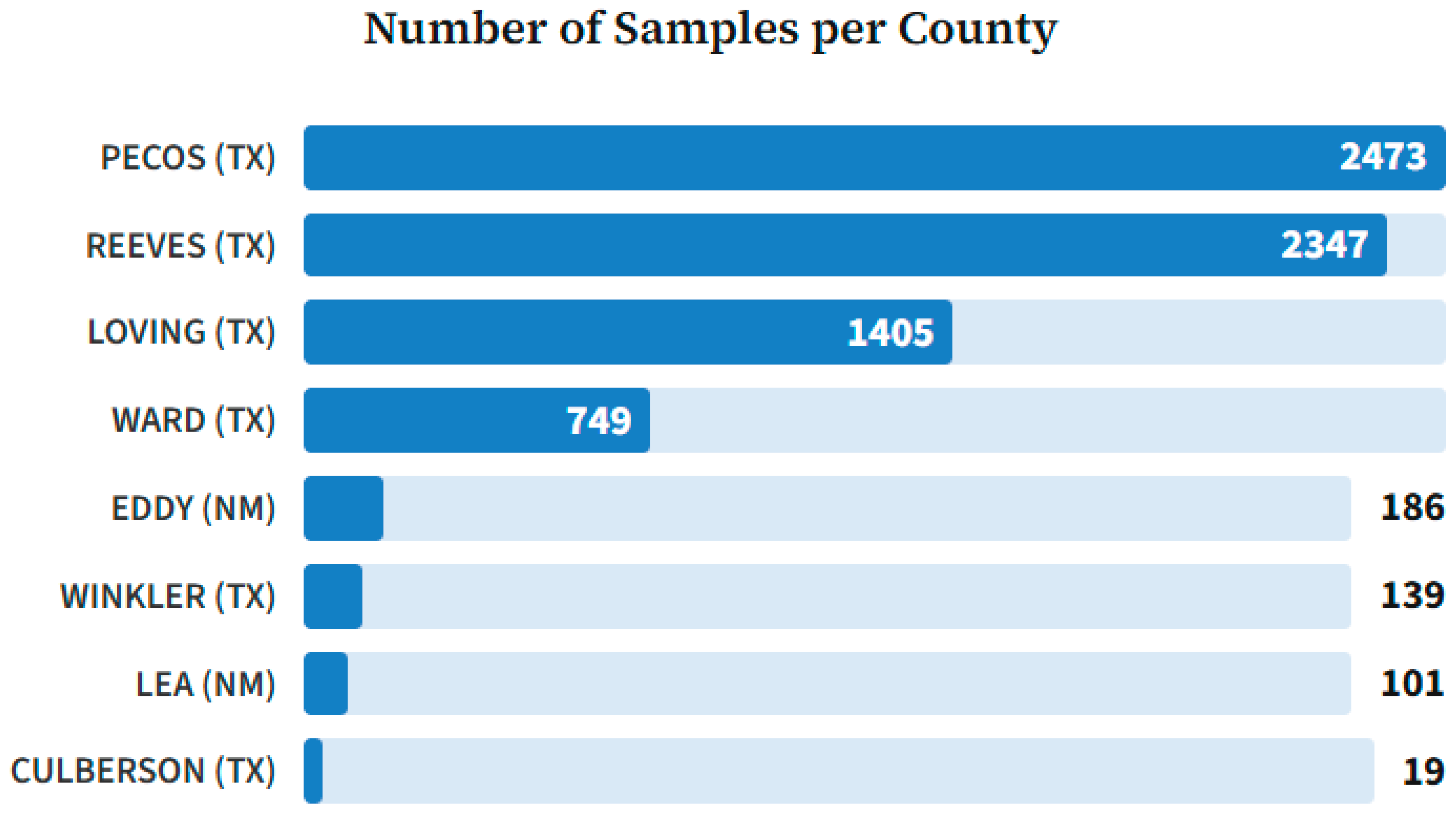
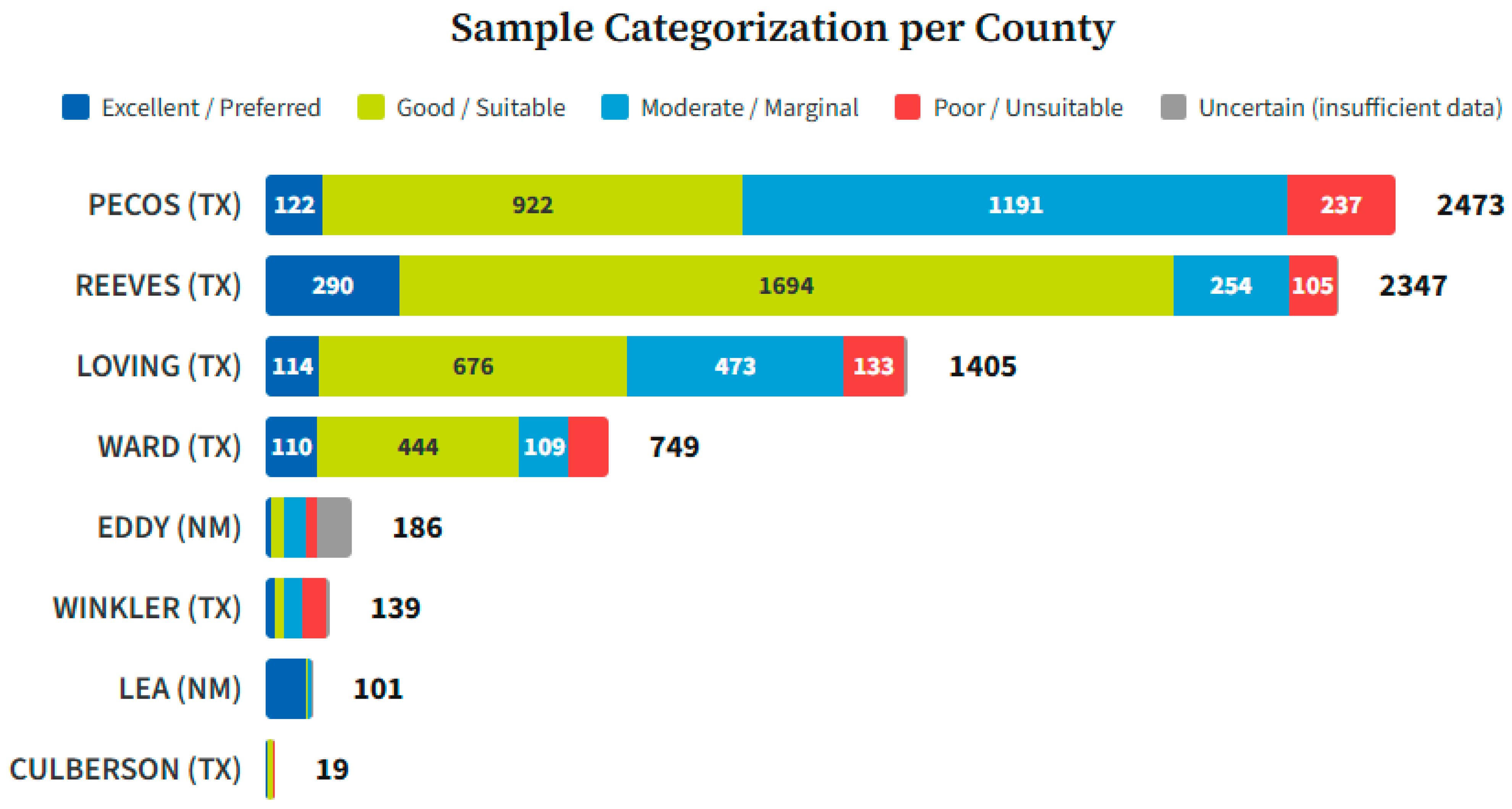
The number of samples used in the geochemical analysis process is dominated by the Pecos and Reeves counties in Texas, with 2473 and 2347 samples each, followed by Loving (1405), Ward (749), Eddy County (186), Winkler (139), Lea (101), and finally, Culberson (19), as can be seen in Figure 8. In addition, the Wolfcamp Formation makes up 4497 samples, followed by the Bone Spring Formation (823), the Delaware Formation (660), the Canyon Formation (614), the Cherry Canyon Formation (186), and the Third Bone Sand Formation (98), as can be seen in Figure 9.

Figure 8. Number of samples per county.

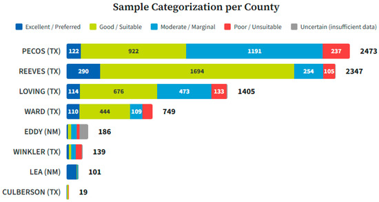
Figure 9. Sample categorization per county.

When interpreted using the three-tier screening system, the samples with TDS < 50,000 mg/L, pH 6–9, and all saturation indices <0.5 are classified as Excellent/Preferred. Samples that are basin in nature and have 50,000 mg/L to 100,000 mg/L of TDS still qualify for reuse and are classified as Good/Suitable. However, samples that exceed the thresholds set in Tier 1 and Tier 2 do not qualify for reuse, particularly those with TDS above 100,000 mg/L. Based on the results obtained from analyzing the PW samples in the Delaware Basin, most of the samples across the Pecos, Reeves, and Loving counties in Texas fall within the Good/Suitable and Moderate/Marginal range, as shown in Figure 9.

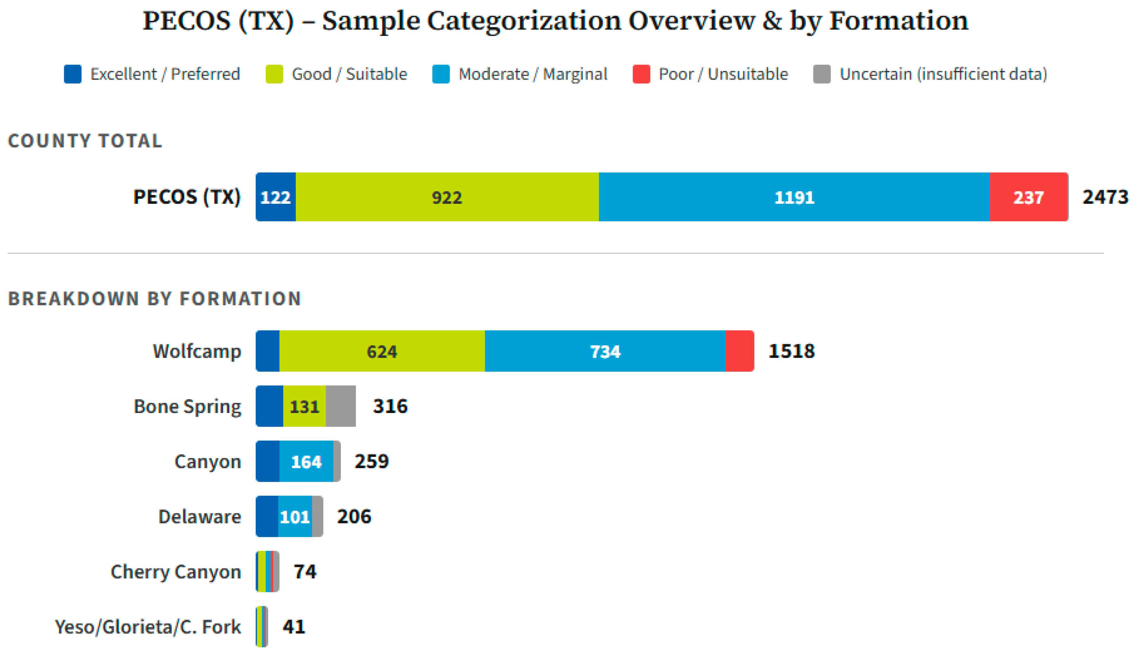
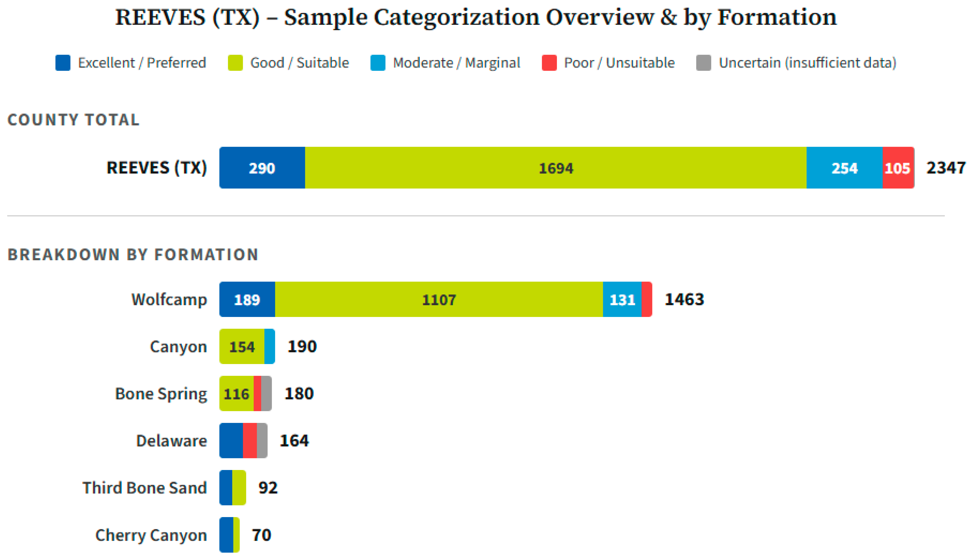
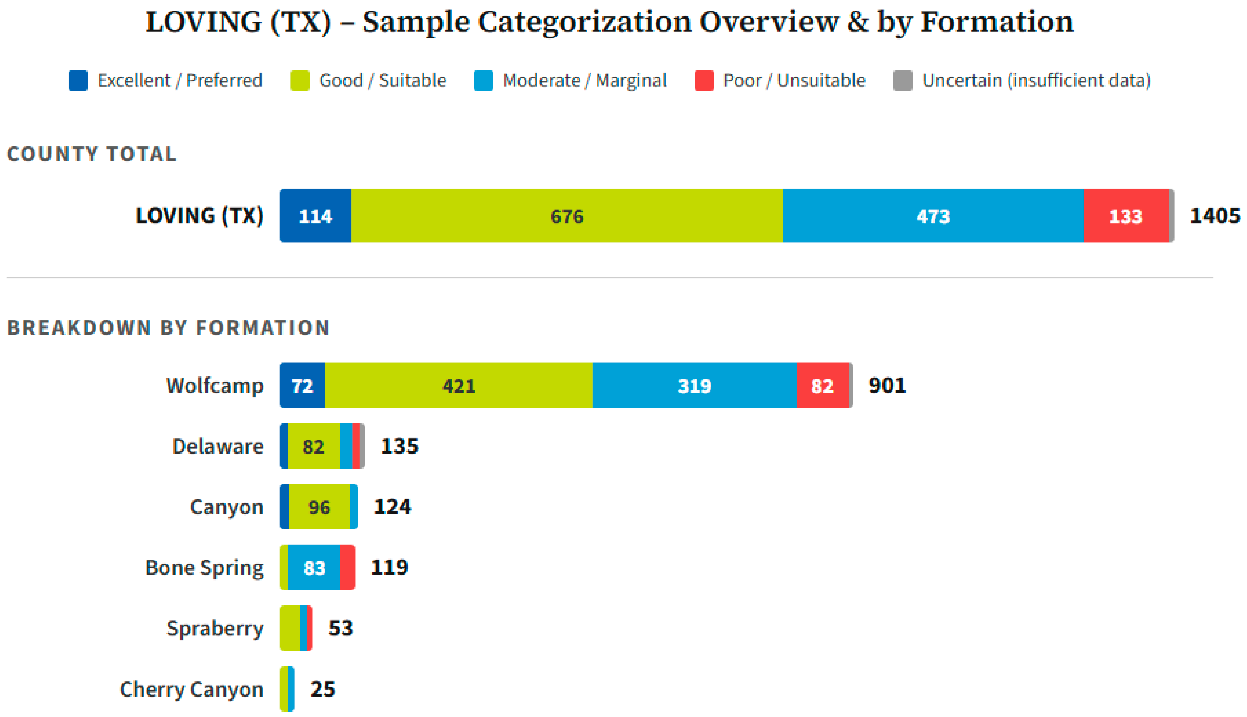
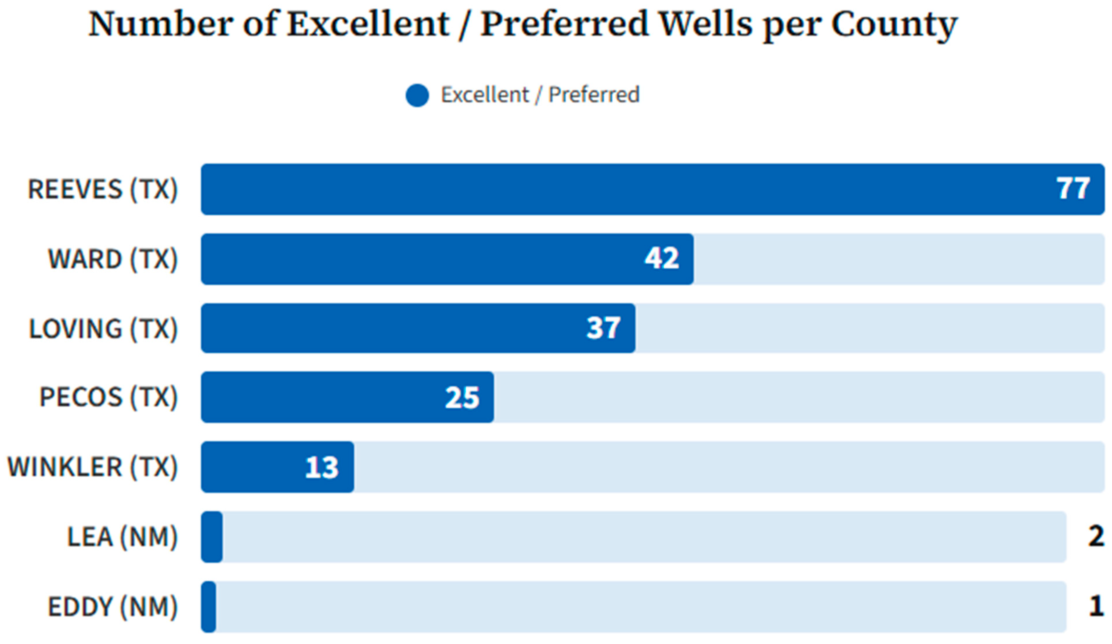
The counties identified as having the best profile based on the geochemical analysis—Eddy and Leah counties in New Mexico, and Loving, Pecos, Reeves, Ward and Winkler in Texas—represent the most productive counties in terms of water production. The Loving, Pecos, and Reeves counties exhibit the largest water producers in the state of Texas, exceeding one billion barrels across a combined 643 wells. Additionally, the results show that a significant number of the samples obtained from the Loving, Pecos, and Reeves counties can be classified as ‘Good/Suitable’ for reproducing across several different formations, with Wolfcamp in the first place, as shown in Figure 10, Figure 11 and Figure 12. It is now important to analyze the future predictions to see whether the best water category wells can produce enough water to be reused in cementing operations.

Figure 10. Sample categorization per formation in Pecos County.

Figure 11. Sample categorization per formation in Reeves County.

Figure 12. Sample categorization per formation in Loving County.

3.2. Produced-Water Availability Forecast

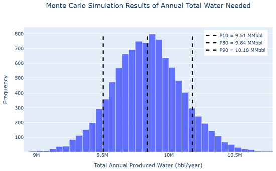
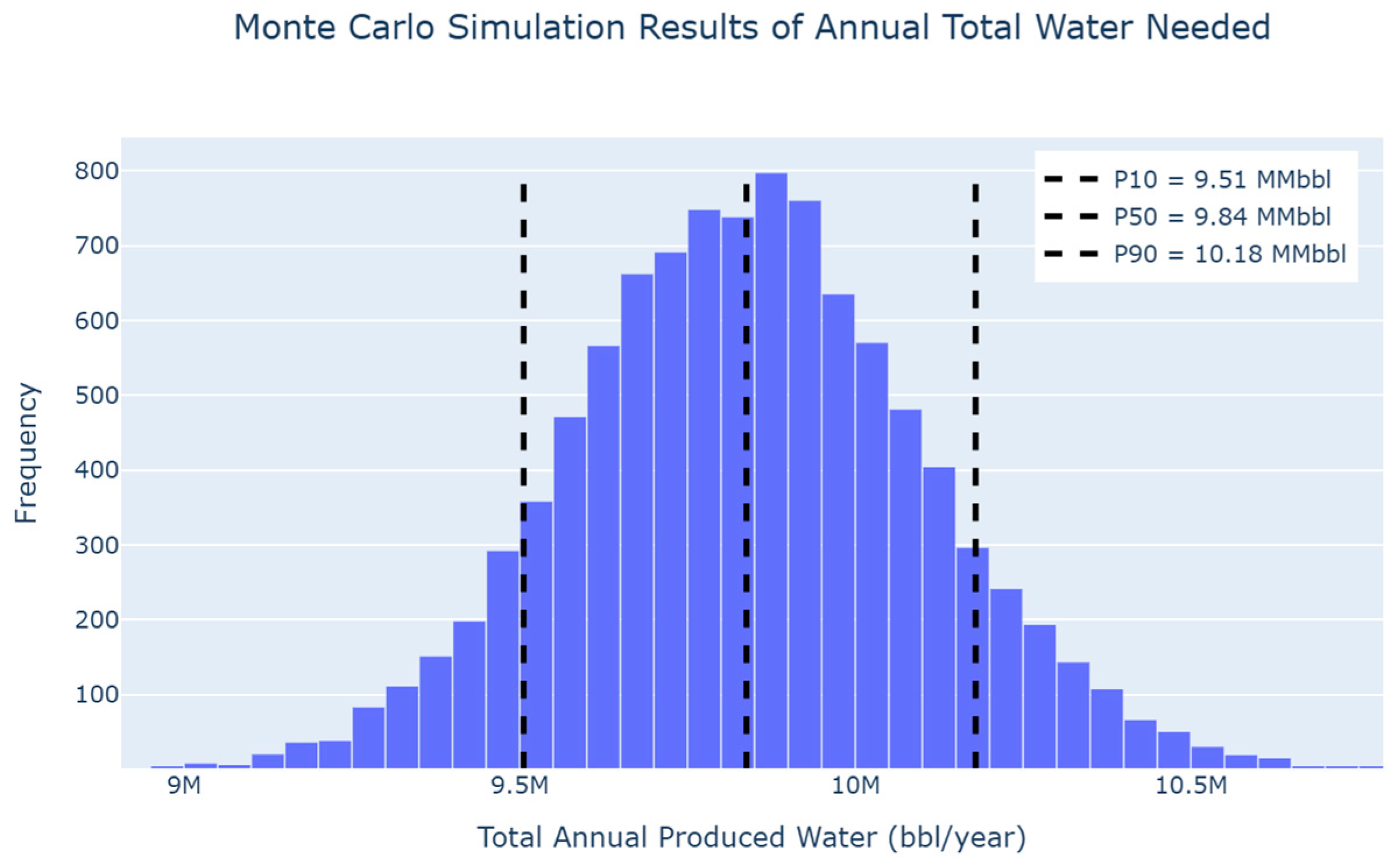
Future water production was estimated using a Monte Carlo simulation, based on well-level forecasts for the 202 wells selected. The cumulative water production was calculated by multiplying the water–oil ratio (WOR) by the estimated ultimate recovery (EUR) of oil for each well, then the resulting values were converted to an annual rate, using the projected production life in months [9]. To account for uncertainty in the forecast, variability was introduced into the process by applying ±20% to WOR, ±15% to EUR, and ±10% to the forecast duration. A total of 10,000 simulations were performed to obtain a probabilistic range of outcomes. The resulting annual water production distribution was summarized, using P10, P50, and P90 values to represent optimistic, median, and conservative scenarios, respectively. The results were then used to compare with the projected cementing water demand. Figure 13 shows the wells identified with excellent samples, and Figure 14’s distribution shows the annual predicted water production.

Figure 13. The wells identified with excellent samples.

Figure 14. The predicted annual water production, according to 10,000 Monte Carlo simulations.

3.3. Identify Future Drilling for Cementing Consumption

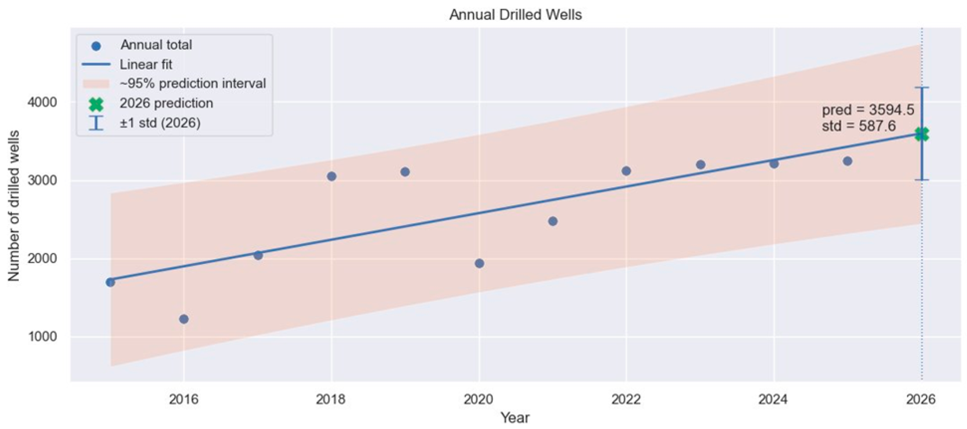
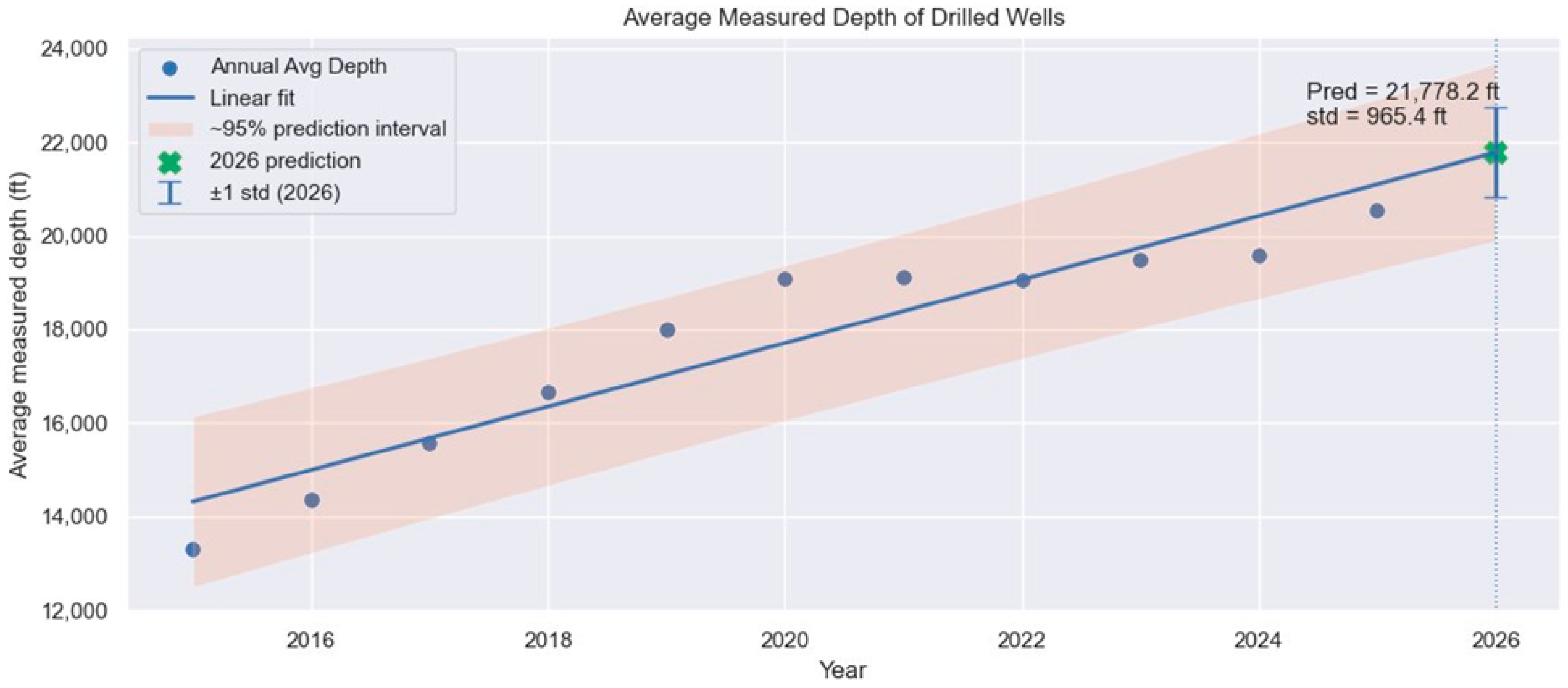
The analysis of the results of water availability depends on the cement water demand, based on the predicted number of wells to be drilled, as well as their average depth. Based on the regression results, the predicted number of drilled wells in 2026 follows a normal distribution with a mean (μ) of 3594.5 wells and a standard deviation (σ) of 587.6 wells, whereas the predicted average depth of the drilled wells was modeled following a normal distribution with a mean (μ) of 21,778.2 ft and a standard deviation (σ) of 965.4 ft.

Figure 15 shows the historical number of drilled wells in the Delaware Basin with a linear regression trend and a 95% prediction interval. The data showcases an overall upward trend in drilling activities, despite some year-to-year fluctuation, especially in the years 2018 to 2020. Based on the fitted model, the predicted number of drilled wells in 2026 is approximately 3594.5 wells, with a standard deviation of about 587.6 wells.

Figure 15. Annual wells drilled (2015–2025) and 2026 prediction in the Delaware Basin.

Figure 16 shows the average measured depth of wells drilled from 2015 to 2026, with the same 95% prediction interval as Figure 8. The projected average depth for 2026 is approximately 21,778 ft, with a standard deviation of about 965 ft.

Figure 16. Average measured depth of drilled wells (2015–2025) and 2026 prediction.

3.4. Future Cementing Water Demand

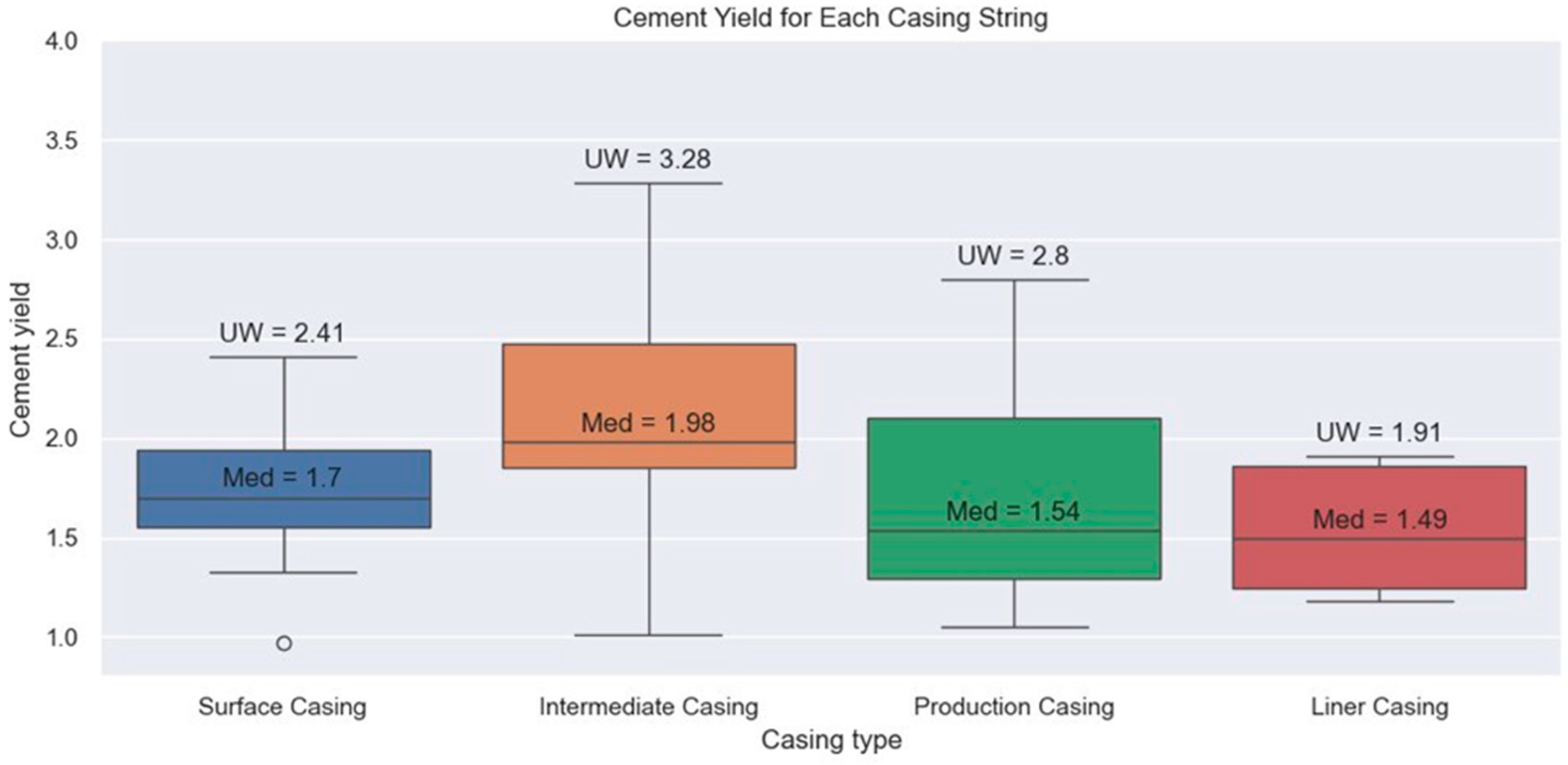
After determining the predicted annual water production and the number of future drillings, the workflow attempts to identify the cement yield for each casing string in order to accurately represent how much cement is required for a well, aiding in determining the water demand. According to the calculations, the intermediate casing shows the median cement yield (≈1.98) and the largest spread, where the UW reaches 3.28. The surface casing comes in second place with a median of 1.7 and an upper whisker of 2.41, indicating a relatively more consistent performance comparatively. The production casing shows a lower median, 1.54, with a wider range than the surface casing, while the liner has the lowest median yield, 1.49. Overall, according to Figure 17, the intermediate casing proves to have the highest demand, which is important when modeling water requirements.

Figure 17. Cement yield per casing string.

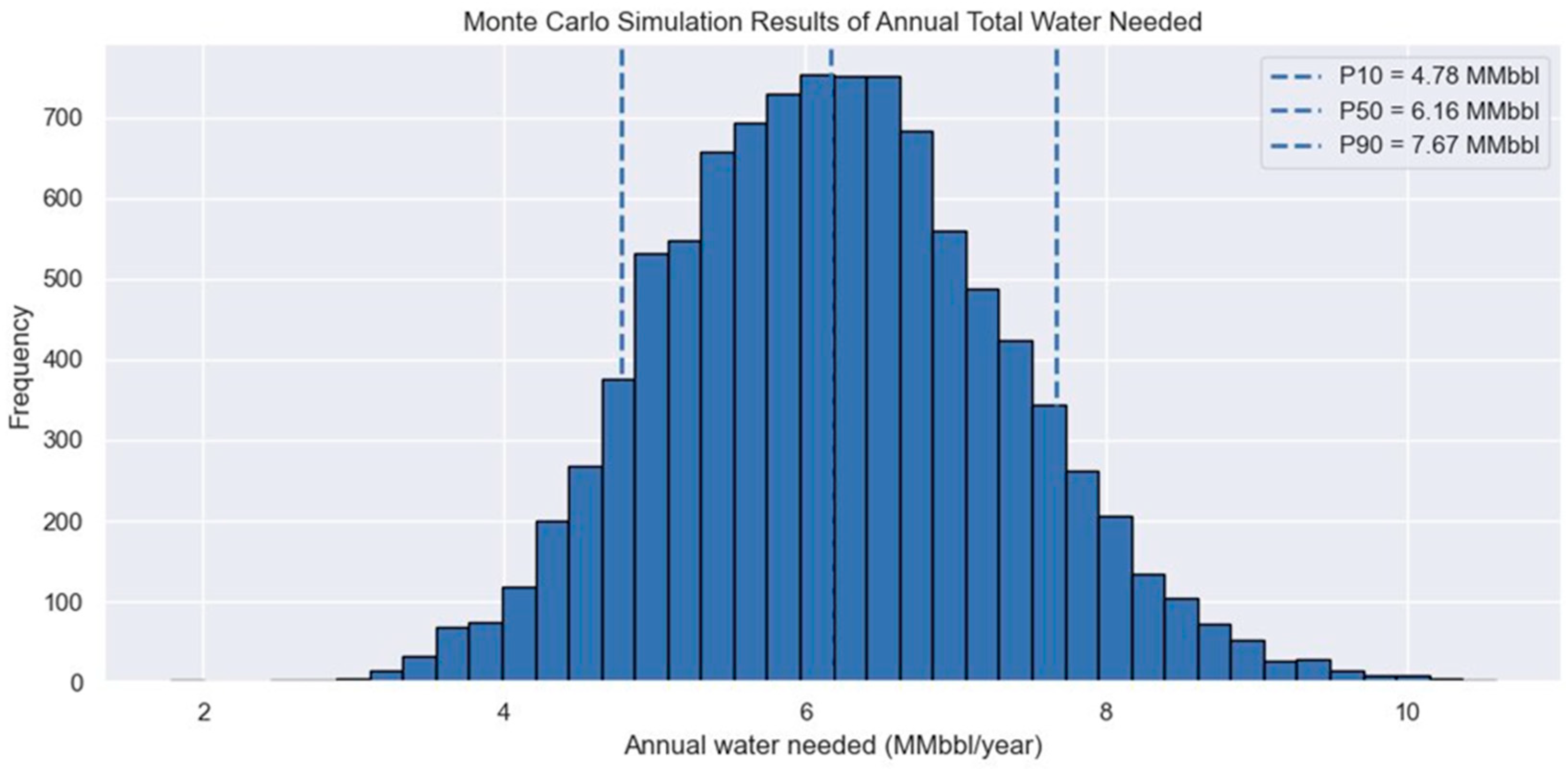
The results of the Monte Carlo simulations indicate that the annual water requirement is likely to center around the P50 value of approximately 6.16 MMbbl/year, shown in Figure 18. As can be seen from the shape of the graph, it is relatively bell-shaped, suggesting moderate uncertainty without any major skewness to either low-case or high-case scenarios. The low-case scenario (P10) estimates 4.78 MMbbl/year, whereas the P90 scenario estimates 7.76 MMbbl/year. The range shows variability in the estimates due to uncertainty in drilling activities, which were predicted in Figure 7 and Figure 8.

Figure 18. Monte Carlo simulation results of the total water demand for cementing operations annually in the Delaware Basin in 2026.

4. Conclusions

In this study, a risk-based framework was developed to evaluate the reuse potential of produced-water in cementing operations in the Delaware Basin. The proposed methodology introduces a three-tier screening system that classifies produced-water into four operational suitability classes, based on geochemical thresholds associated with cement performance risks. The application of the framework shows that a significant volume of produced water in the highest producing counties in the Delaware Basin, including the Loving, Pecos, Reeves, Eddy, and Lea counties, falls within the Excellent/Preferred and Good/Suitable categories, indicating strong technical potential for reuse with minimal chemical conditioning.

To evaluate the long-term feasibility, a Monte Carlo forecasting approach was used to estimate the water demand and future produced-water availability. The results predict a median (P50) cement water demand of 6.16 MMbbl/year, while accounting for uncertainties in both drilling and well depth. Forecasted produced-water volumes classified as Excellent/Preferred and Good/Suitable were found to be sufficient for the demand, even under conservative conditions in which the water demand was overestimated.

The novelty of this study lies in combining geochemical risk screening, operational suitability classification, and probabilistic forecasting into a single workflow for produced-water reuse evaluation. This approach provides a practical and easy-to-use decision-support tool that enables operators to customize the process according to their water availability and requirements. The results confirm that the reuse of produced water in cementing operations in the Delaware Basin is a viable option, is operationally scalable, and is capable of reducing the consumption of freshwater.

References

- Hennings, P. The Geology of Injection-Induced Earthquakes in the Midland Basin Region: Introduction. AAPG Bull. 2024, 108, 2195–2200. [Google Scholar] [CrossRef] [Scilit]
- Wang, Z.; Wang, C.; Meng, L.; Qi, X.; Hong, J. Prediction of Sump Oil Growth Rate towards Gravitational Settling of Produced Water in Oilfield Based on Machine Learning. Desalination Water Treat. 2024, 317, 100189. [Google Scholar] [CrossRef] [Scilit]
- Skoumal, R.J.; Barbour, A.J.; Brudzinski, M.R.; Langenkamp, T.; Kaven, J.O. Induced Seismicity in the Delaware Basin, Texas. J. Geophys. Res. Solid Earth 2020, 125, e2019JB018558. [Google Scholar] [CrossRef] [Scilit]
- Ge, J.; Nicot, J.-P.; Hennings, P.H.; Smye, K.M.; Hosseini, S.A.; Gao, R.S.; Breton, C.L. Recent Water Disposal and Pore Pressure Evolution in the Delaware Mountain Group, Delaware Basin, Southeast New Mexico and West Texas, USA. J. Hydrol. Reg. Stud. 2022, 40, 101041. [Google Scholar] [CrossRef] [Scilit]
- Bruant, R. The Growing Pressures of Produced Water Disposal. Available online: https://jpt.spe.org/the-growing-pressures-of-produced-water-disposal?utm_source=chatgpt.com (accessed on 3 February 2026).
- RRC. Permian Disposal Wells Guidance Release. Available online: https://www.rrc.texas.gov/news/05162025-permian-disposal-wells-guidance-release/?utm_source=chatgpt.com (accessed on 3 February 2026).
- Parastatidis, E.; Averett, A.; Sarkis, P.; Salles, V.; Huang, D.; Vallejo, K.; Eichhubl, P.; Bhattacharya, S.; Bakirtzis, N.; Kalogirou, E.; et al. 2024 Biennial Report on Seismic Monitoring and Research in Texas; Bureau of Economic Geology: Austin, TX, USA, 2024. [Google Scholar]
- Skoumal, R.J.; Kaven, J.O.; Barbour, A.J.; Wicks, C.; Brudzinski, M.R.; Cochran, E.S.; Rubinstein, J.L. The Induced Mw 5.0 March 2020 West Texas Seismic Sequence. J. Geophys. Res. Solid Earth 2021, 126, e2020JB020693. [Google Scholar] [CrossRef] [Scilit]
- Enverus, D. DrillingInfo, Enverus. Available online: https://www.enverus.com/about-enverus/ (accessed on 13 February 2026).
- Omoniyi, O.A.; Anas, K.; Abba, M.K. Comparing the Effect of Saline Water and Fresh Water on Oil Well Cementing Properties. Int. J. Innov. Res. Sci. Eng. Technol. 2007, 5, 8430–8440. [Google Scholar] [CrossRef]
- Zhang, J.; Weissinger, E.A.; Peethamparan, S.; Scherer, G.W. Early Hydration and Setting of Oil Well Cement. Cem. Concr. Res. 2010, 40, 1023–1033. [Google Scholar] [CrossRef] [Scilit]
- Yousuf, N.; Olayiwola, O.; Guo, B.; Liu, N. A Comprehensive Review on the Loss of Wellbore Integrity Due to Cement Failure and Available Remedial Methods. J. Pet. Sci. Eng. 2021, 207, 109123. [Google Scholar] [CrossRef] [Scilit]
- Asadov, S.; Ozyurtkan, M.H. Modelling the Effect Additives on Exothermic Heat Development of Well Cement. In ARMA US Rock Mechanics/Geomechanics Symposium; ARMA: Overland Park, KS, USA, 2017; p. ARMA-2017. [Google Scholar]
- Matovu, S.; Abdulhamid, A.; Talal, M.; Shafloot, A. High-Performance Lightweight Cements: A Review. In ARMA US Rock Mechanics/Geomechanics Symposium; ARMA: Overland Park, KS, USA, 2024. [Google Scholar]
- Ahmed, A.; Mohamed, A.; Elkatatny, S. The Perlite Usage in High Density Oil-Well Cement. In ARMA US Rock Mechanics/Geomechanics Symposium; ARMA: Overland Park, KS, USA, 2024. [Google Scholar] [CrossRef] [Scilit]
- Adjei, S.; Elkatatny, S. Overview of the Lightweight Oil-Well Cement Mechanical Properties for Shallow Wells. J. Pet. Sci. Eng. 2021, 198, 108201. [Google Scholar] [CrossRef] [Scilit]
- Liu, G. Applied Well Cementing Engineering; Gulf Professional Publishing: Cambridge, MA, USA, 2021. [Google Scholar]
- Broni-Bediako, E.; Kove, E.P.A. The Effect of Water-Cement Ratio and Temperature on Density and Rheological Properties of Oil Well Cement Slurry. Int. J. Emerg. Sci. Eng. 2025, 13, 1–7. [Google Scholar] [CrossRef] [Scilit]
- Cadix, A.; Hernandez, M.; Blaizot, D.; Thant, K.P. Cementing Geothermal Wells with Adapted Cementitious Materials: Formulation and Additives Selection. In Proceedings of the SPE International Symposium on Oilfield Chemistry; Society of Petroleum Engineers (SPE): Richardson, TX, USA, 2023. [Google Scholar]
- Samsuri, A.; Phuong, B.T.N. Cheaper Cement Formulation for Lost Circulation Control. In IADC/SPE Asia Pacific Drilling Technology; SPE: Richardson, TX, USA, 2002. [Google Scholar] [CrossRef]
- Brother, L.; de Blanc, F.; Services, H. New Cement Formulation Helps Solve Deep Cementing Problems. J. Pet. Technol. 1989, 41, 611–614. [Google Scholar] [CrossRef] [Scilit]
- Bechara, E.; Watson, M.; Arbad, N. Unlocking Sustainability: Transforming Tight-Oil Produced Water into a Lifeline for West Texas. Environ. Process. 2024, 11, 26. [Google Scholar] [CrossRef] [Scilit]
- RRC. Public GIS Viewer. Available online: https://www.rrc.texas.gov/resource-center/research/gis-viewer/ (accessed on 13 February 2026).
- Oil Conservation Division OCD Permitting. Available online: https://wwwapps.emnrd.nm.gov/OCD/OCDPermitting/Data/Wells.aspx (accessed on 13 February 2026).
- Das, K.K.; Wu, X.; Noh, G.; Lee, J.H.; Jang, J.G. Effect of Acid Attack Coupled with Elevated Temperatures on Carbonation-Cured Calcium Sulfoaluminate and Ordinary Portland Cement Paste. Case Stud. Constr. Mater. 2025, 23, e05150. [Google Scholar] [CrossRef] [Scilit]
- Peng, H.; Xu, Z.D.; Xia, Z.; Zang, X.; Xi, D.; Jiang, X.; Zhao, W.; Lu, H. Closed Wellbore Integrity Failure Induced by Casing Corrosion Based on Solid-Chemical Coupling Model in CO2 Sequestration. Geoenergy Sci. Eng. 2024, 241, 213140. [Google Scholar] [CrossRef] [Scilit]
- Angst, U.M.; Boschmann, C.; Wagner, M.; Elsener, B. Experimental Protocol to Determine the Chloride Threshold Value for Corrosion in Samples Taken from Reinforced Concrete Structures. J. Vis. Exp. 2017, 2017, e56229. [Google Scholar] [CrossRef] [Scilit]
- Mousavinezhad, S.; Toledo, W.K.; Newtson, C.M.; Aguayo, F. Rapid Assessment of Sulfate Resistance in Mortar and Concrete. Materials 2024, 17, 4678. [Google Scholar] [CrossRef] [Scilit]
- Zheng, Y.; Mei, K.; Wei, T.; He, X.; Liu, C.; Zhang, C.; Cheng, X. Calcined Mg-Rich Olivine Enhanced Oil-Well Cement for Anti-Supercritical CO2 Invasion under the High-Temperature and High-Pressure Conditions. Geoenergy Sci. Eng. 2025, 252, 213914. [Google Scholar] [CrossRef] [Scilit]
- Eyu, G.D.; Will, G.; Dekkers, W.; MacLeod, J. Effect of Dissolved Oxygen and Immersion Time on the Corrosion Behaviour of Mild Steel in Bicarbonate/Chloride Solution. Materials 2016, 9, 748. [Google Scholar] [CrossRef] [Scilit]
- Mao, H.; Wang, W.; Ma, Y.; Huang, Y. Synthesis, Characterization and Properties of an Anionic Polymer for Water-Based Drilling Fluid as an Anti-High Temperature and Anti-Salt Contamination Fluid Loss Control Additive. Polym. Bull. 2021, 78, 2483–2503. [Google Scholar] [CrossRef] [Scilit]
- Anya, F.; Anaele, J.V.; Usiayo, V.A. Investigation of the Effect of Water Salinity on the Thickening Time of Cement Slurry. Int. J. Res. Innov. Appl. Sci. 2025, 10, 1428–1434. [Google Scholar] [CrossRef] [Scilit]
- Wang, Y.; He, F.; Wang, J.; Wang, C.; Xiong, Z. Effects of Calcium Bicarbonate on the Properties of Ordinary Portland Cement Paste. Constr. Build. Mater. 2019, 225, 591–600. [Google Scholar] [CrossRef] [Scilit]
- Yan, Y.; Yu, T.; Song, J.; Wu, B.; Qu, C. A Review of Prediction Methods for Oilfield Produced Water Scaling. In Proceedings of the IOP Conference Series: Earth and Environmental Science; IOP Publishing Ltd.: Bristol, UK, 2021; Volume 651. [Google Scholar]
- Guichet, X.; Jouniaux, L.; Catel, N. Modification of Streaming Potential by Precipitation of Calcite in a Sand-Water System: Laboratory Measurements in the PH Range from 4 to 12. Geophys. J. Int. 2006, 166, 445–460. [Google Scholar] [CrossRef] [Scilit]
- Nelson, E.B.; Guillot, D. Well Cementing; Schlumberger: Paris, France, 2006. [Google Scholar]
- Habibi, A.; Fensky, C.E.; Roostaei, M.; Mahmoudi, M.; Fattahpour, V.; Zeng, H.; Sadrzadeh, M. A Laboratory Workflow for Characterization of Scaling Deposits in Thermal Wells. Energies 2020, 13, 3184. [Google Scholar] [CrossRef] [Scilit]
- Cather, M.; Lee, P.R.; Gundiler, P.M.I.; Sung, C.-P.A.; Davidson, N.; Reddy, A.K.; Wei, M. NM WAIDS: A Produced Water Quality and Infrastructure GIS Database for New Mexico Oil Producers (FINAL Technical Progress Report); New Mexico Institute of Mining and Technology: Socorro, NM, USA, 2005. [Google Scholar]
- Taylor, H.F.W. Cement Chemistry; Thomas Telford: London, UK, 1998. [Google Scholar]
- Smith, D.K. Cementing; H.L. Doherty Memorial Fund of AIME: Richardson, TX, USA, 1976. [Google Scholar]
- Parkhurst, D.; Appelo, C. Description of Input and Examples for PHREEQC Version 3—A Computer Program for Speciation, Batch-Reaction, One-Dimensional Transport, and Inverse Geochemical Calculations; U.S. Geological Survey: Reston, VA, USA, 2013. [Google Scholar]
Disclaimer/Publisher’s Note: The statements, opinions and data contained in all publications are solely those of the individual author(s) and contributor(s) and not of MDPI and/or the editor(s). MDPI and/or the editor(s) disclaim responsibility for any injury to people or property resulting from any ideas, methods, instructions or products referred to in the content. |
© 2026 by the authors. Licensee MDPI, Basel, Switzerland. This article is an open access article distributed under the terms and conditions of the Creative Commons Attribution (CC BY) license.